Submitted to

Faculty of Technology and Maritime Sciences, University of Southeast Norway,

in partial fulfilment of the requirements for the degree

Joint International Master in Smart Systems Integration (SSI)

MASTER THESIS

Ultrasound Transducer Design for

Continuous Fetal Heartbeat Monitoring

by Assel Rakhmetova

This work has been carried out at HSN, Department of Micro- and Nanosystem

Technology, under the supervision of

Associate Professor Kristin Imenes

Vestfold, 4 July 2016

Abstract

Stillbirth prevention requires high quality healthcare and early detection. Continuous

monitoring of fetal heartbeat can be one of the ways to reduce pregnancy complications

and even stillbirths. A Doppler ultrasound transducer is found to be one of the possible

devices that can be adopted for home long-term monitoring of the fetal heartbeat.

Computer simulations and laboratory work were conducted to research a question of

continuous monitoring of the fetal heart with the use of the Doppler transducer.

Simulations were performed in MATLAB and Field II software environments. B-mode

and M-mode images of the heart phantom were created with changed positions and

amplitudes of the scatterers to imitate movements of the tissue structure. The received

signals from the moving scatterers are then analyzed and time shifts are extracted.

Transducer aperture was varied in order to increase transducer robustness for the

application. Phantom position was changed in x- and z-directions. This allowed

simulating the cases when either position of the transducer is displaced or fetus moves.

Laboratory work was performed to create a test environment with a transmit/receive

hardware system and a single-element transducer. LabVIEW graphical software was

used to drive the hardware electronics. This test environment was performed to

understand functioning of the transducer and the system in a real-time performance.

The velocity of the heart phantom was obtained from the time shifts between the

consecutive received signals. It was possible to measure the heart velocity if the heart

position is changed from the central lobe of the transducer beam in x-direction.

However, the measurements are not accurate if the radius of the transducer aperture is

decreased to 2 mm. The measured velocity of the heart phantom is in a good agreement

with the actual velocity if heart is moved in z-direction. However, the received RF

signals from the back heart wall are much weaker as compared to the received signals

for the front heart wall.

The proposed idea to have a continuous fetal heartbeat monitoring is found to be one of

the solutions to reduce number of stillbirths. Doppler transducer shows improved

robustness with decreased size of the aperture which lead to a wider beam profile and

better detectability of the heart movements.

Dedicated to my stillborn daughter named Aisha,

who is always in my heart

Acknowledgements

I am very thankful to my supervisor Dr. Kristin Imenes, who supported my idea to

propose a topic for a master thesis and who agreed to lead me all those months of the

hard work. I am also very thankful to Prof. Lars Hoff and his ultrasound group who

helped me to understand a new field for me –Acoustics.

I appreciate all my teachers in the Department of Micro- and Nanosystem Technology,

who are the greatest and the kindest lecturers I had in my life.

I would like to express special thank you to Merete Hovet. She became my second

mother during the whole SSI program. I express my sincere gratitude to Prof. Knut

Aasmundtveit for his great support throughout all two years of the master program.

I am very thankful to midwives and doctors in Horten Kommune Helsestasjon,

especially Hilde Haug for her time and guidance.

My sincere gratitude goes to my parents, sisters, friends and groupmates for their

endless love and support.

Acronyms

2D Two Dimensional

AFI Amniotic Fluid Index

Bpm Beats per minute

D Diastole

DRM Detection and Recording Module

FDA Food and Drug Administration

LV Left Ventricle

MI Mechanical Index

N Number of scatterers

PDM Processing and Display Module

RF Radio Frequency

RV Right Ventricle

S Systole

SFH Symphysis-Fundal Height

Table of Contents

1 Introduction ................................................................................................................................................ 1

1.1 Problem Statement ......................................................................................................................... 1

1.2 Objective of the Study .................................................................................................................... 2

1.3 Research Questions ........................................................................................................................ 2

1.4 Thesis Organization ........................................................................................................................ 3

2 Literature Background ............................................................................................................................ 4

2.1 Pregnancy Evaluation Tests ........................................................................................................ 4

2.2 Pregnancy Evaluation Tests for Home Monitoring ........................................................... 9

2.3 Fetal Heartbeat Monitoring Systems .................................................................................... 12

3 Theoretical Background ....................................................................................................................... 13

3.1 Physics of Ultrasound .................................................................................................................. 13

3.1.1 Reflection and Transmission ........................................................................................... 14

3.1.2 Scattering ................................................................................................................................. 15

3.1.3 Attenuation .............................................................................................................................. 16

3.2 Ultrasound Transducers ............................................................................................................. 17

3.3 Ultrasound Imaging ...................................................................................................................... 19

3.4 Principles of Doppler Ultrasound ........................................................................................... 20

3.4.1 The Doppler Effect ............................................................................................................... 20

3.4.2 Continuous-wave and Pulse-wave Doppler .............................................................. 21

3.5 Ultrasound Safety .......................................................................................................................... 22

3.5.1 Thermal Effects ...................................................................................................................... 22

3.5.2 Non-thermal effects ............................................................................................................. 23

4 Methodology ............................................................................................................................................. 24

4.1 MATLAB and FIELD II Summary ............................................................................................. 24

4.2 Fetus and Pregnant Woman Design Parameters ............................................................. 26

4.3 Simulation Design .......................................................................................................................... 29

4.3.1 Ultrasound Transducer Design Model ......................................................................... 29

4.3.2 Heart Model ............................................................................................................................. 30

4.3.3 Simulation model .................................................................................................................. 33

4.4 Laboratory work ............................................................................................................................ 38

5 Results ......................................................................................................................................................... 40

5.1 B-mode Heart Image .................................................................................................................... 40

5.2 Case studies ...................................................................................................................................... 41

5.2.1 Case study A ............................................................................................................................ 44

5.2.2 Case study B ............................................................................................................................ 50

5.2.3 Case Study C ............................................................................................................................ 54

5.2.4 Case study D ............................................................................................................................ 61

5.3 Laboratory work ............................................................................................................................ 64

6 Discussion .................................................................................................................................................. 67

6.1 Simulations ....................................................................................................................................... 68

6.1.1 Case study A and B ............................................................................................................... 68

6.1.2 Case study C and D ............................................................................................................... 70

6.2 Laboratory work ............................................................................................................................ 72

6.3 Ultrasound safety........................................................................................................................... 72

7 Conclusion And Future Work ............................................................................................................. 73

Glossary ................................................................................................................................................................ 74

Appendix A: MATLAB code for a Heart Phantom Image .................................................................. 75

Appendix B: MATLAB codes used for Case Study A, B, C & D ......................................................... 80

Appendix C: MATLAB code for M-Mode Image .................................................................................... 82

Appendix D: Piston Transducer Beam Profile ...................................................................................... 83

Appendix E: Flat LABVIEW ‘Process’ State ............................................................................................ 83

References ........................................................................................................................................................... 85

List of Figures .................................................................................................................................................... 92

List of Table ........................................................................................................................................................ 96

1

1 INTRODUCTION

1.1 Problem Statement

Many women and children still die during the pregnancy. It is estimated that

there are 303 000 maternal deaths and 2.6 millions of stillbirths in the world registered

in 2015. Every day 7 300 women suffer the loss of their babies in the last three months

of gestation [1]. Stillbirth is a baby born with no signs of life after 28 weeks of

pregnancy[2]. There are more than 3600 cases of stillbirths every year in the UK. Eleven

babies die every day and one in every 200 labours ends up in a stillbirth [3].

Stillbirth prevention requires high quality healthcare, early detection and

diagnosis. It is not affordable in many countries and especially not in developing low-

income countries. The majority of stillbirths are preventable and it mostly depends on

the access to maternal healthcare and immediate diagnosis of possible complications.

Various pregnancy-monitoring tests are usually performed to control normal

and high-risk pregnancy in women. Sometimes, additional tests of fetal well-being may

be needed to predict and to prevent serious pregnancy complications and even

stillbirth. However, none of the traditional tests have a definitely proven effect when it

comes to decreasing intrauterine stillbirths [4].

Moreover, for women with no signs of problems during the pregnancy, such tests

are not usually performed. Not detecting pregnancy complications can lead to critical

incidents and, for women in their first pregnancy, even sudden fetus death can occur.

Also, these tests require the woman to come to hospital twice a week (or more) which

can be inconvenient for some women who have health problems. Perhaps most

importantly, the fetus is not observed in between the tests which brings difficulties to

catch any fetal disorders.

There is no sole strategy to predict a stillbirth [5]. For example, if a pregnant

woman feels less baby movements inside the uterus, the non-stress test and ultrasound

related tests will be performed to assess fetus health at the moment [6], [7]. The fetal

can behave healthy at the moment of the screening. However, the well-being of the fetus

can change later once woman has left the hospital. One of the reasons for a stillbirth can

2

be an infection. This includes bacterial infections (Escherichia coli, streptococcus),

viruses (parvovirus B19) or parasites (toxoplasmosis, malaria) [5]. However, if a

woman complains about the decrease of the baby movements, blood, urine and vaginal

tests are not performed to diagnose for the presence of any infections. Existing Doppler

instruments for heartbeat listening that can be used by woman at home to listen to a

fetal heartbeat cannot be used as medical devices to evaluate any fetal abnormalities.

Moreover, these instruments can be used improperly leading to false measurements [8].

They are rather used by midwives as a psychological tool to instill future mothers with

an idea of having a baby in the near future.

1.2 Objective of the Study

The objective of the study is to investigate the possibility of having a continuous

monitoring system to record a fetal heartbeat during the third gestation trimester to

prevent stillbirth. The objective may be fulfilled by designing an ultrasound transducer

with a suitable analysis system that can be attached to a woman abdomen to

continuously monitor a fetal heartbeat.

1.3 Research Questions

The diagnostic ultrasound is a noninvasive and safe technique used in clinical

practice. It has also advantages of low cost and portability. The future of ultrasound

systems to be miniature, mobile and portable is improving and promising.

A fetal heartbeat continuous monitoring system can be implemented by a well-

established technique called Doppler ultrasound. The question arises whether

traditional Doppler ultrasound techniques can be adopted for continuous evaluation of

the fetal heartbeat and be used at home for long term monitoring. Will it always be

possible to catch the fetal heartbeat during the long term screening if a transducer is

attached on the female abdomen?

Another issue is whether continuous heartbeat monitoring can help to reduce

stillbirth accidents. Can we rely on the heartbeat as a reflection of the fetus well-being

status?

3

It is also important to investigate whether there are any bio-effects of the

ultrasound if a fetus is exposed to it throughout a day. Will it be safe for a baby and the

mother?

1.4 Thesis Organization

Thesis consists of literature background, theoretical overview, methodology,

results, discussion, conclusion and future work chapters. Literature background

introduces current pregnancy evaluation tests that available in hospitals and on the

market. It also discusses their limitations and drawbacks. Theoretical background gives

an overview of the ultrasound physics that is used to build a single-element transducer

and to analyze Doppler ultrasound theory. Methodology describes case studies design

parameters that were created to investigate problem stepwise. Results and discussion

chapters introduce main theoretical and experimental results and discuss their

outcomes. Conclusion and future work chapter summarizes the work performed and

proposes the future improvements and development of the topic.

4

2 LITERATURE BACKGROUND

2.1 Pregnancy Evaluation Tests

Usually, pregnant woman does not need to have any extra check-ups during her

pregnancy unless there are pre-existing health conditions which may cause miscarriage

and even stillbirth.

The possible reasons causing stillbirth include[2],[3], [5], [9]:

childbirth complications

infections during the pregnancy

maternal disorders (hypertension, diabetes)

fetal growth restrictions

congenital abnormalities

It is important to perform the examination of fetus well-being in high risk

pregnancies for women who have [10],[11]:

complications in the previous pregnancies or stillbirth

existing health conditions such as diabetes, heart disease

complications during pregnancy such as fetal growth problems, placenta

abnormalities

decreased fetal movement, fetal hypoxia

prolonged pregnancy (beyond 40 weeks)

Certain evaluation tests may be used to assess fetal well-being which are

performed in hospital if woman experiences less fetal movements or she has above

mentioned health conditions [4], [12]:

fetal movement assessment

non-stress test including uterine contraction test

amniotic fluid index

contraction stress test

biophysical profile

umbilical artery Doppler

5

Fetal movement assessment [13] is a routine method used to monitor normal

pregnancy. It is also a method that can be used in high risk pregnancy. Fetal movement

assessment is a method when woman counts the number of kicks or movements of a

baby during the day. Usually woman can feel the baby`s movement from 20-24 weeks of

gestation. According to several studies, there should be at least 10 distinct baby

movements in 11-34 minutes. If a woman feels or counts a decreased number of

movements then she must take more tests to evaluate fetus well-being. However,

sometimes woman may feel anxious while counting the movements, which may be

destructive to accomplish the test. Also, some woman can be busy at work or with other

children during the day and they are not able to monitor baby`s activity [12], [14].

Pregnant women have to select two hours during a day when the baby is the most active

to count the fetal movements [13].

Non-stress test (cardiotocography) [12][15] – is a non-invasive test widely used

in obstetrics. The principle of the test is the association of the fetal heart rate with fetal

movements. Healthy babies will have an increase in the heart rate while moving, and a

reduction in the heart rate while at rest.

Figure 2-1 illustrates the basic set-up of the monitoring system usually installed

for non-stress test. The set-up consists of the ultrasound system, tokodynamometer and

auxiliary electronics. The ultrasound system utilizes Doppler ultrasound (Doppler

effect) and records the heartbeat of the fetus. Tokodynamometer [16] is a pressure

transducer placed around a woman`s abdomen with an elastic belt. When the uterine

muscles contract, they raise the abdominal wall depressing the plunger and intrauterine

pressure is measured.

Figure 2-1: Fetal monitoring system. An ultrasound transducer measures fetal heartbeat

while a tokodynamometer measures uterine activity [17].

6

It requires 20-40 minutes to complete the test. The test is performed as frequent

as required for high-risk pregnancies. Usually, pregnant women are asked to eat before

the test as it can make the baby move more actively. During the test, the woman lies on

her side while the ultrasound system and the tokodynamometer are attached around

woman`s abdomen by elastic belts. The woman is asked to press a button when she

feels a movement. There are two results of the test: reactive and non-reactive. Reactive

means that the baby`s heart rate increases as the baby moves. There should be an

increase of the fetal heart rate of 15 bpm from the baseline for 15 seconds occurring

two or more times during a 20 or 30 minutes period in conjunction with fetal

movement. Non-reactive means the baby`s heart rate does not increase as the baby

moves. Figure 2-2 shows an example of a non-stress test result provided by the

“Sykehuset i Vestfold” hospital.

Figure 2-2: Non-stress test shows normal fetal heart rate accelerations.

Amniotic fluid index (AFI) [12], [18] - is an ultrasound measurement technique

of amniotic fluid volume. The uterus is divided into four quadrants and the largest

vertical amniotic fluid pocket in each quadrant is measured. AFI is the sum of these four

measurements. In the third trimester AFI is between 8 and 25 cm.

Olygohydraminos is defined for AFI less than 5 cm and associated with increase

of caesarean section for fetal distress.

7

Polyhydramios is defined for AFI which is greater than 25 cm and associated

with an increase of perinatal mortality rate, fetal abnormalities, increased caesarean

ection rate.

Contraction stress test [19]- is an invasive procedure which is performed to

evaluate the fetus response to the stimulated uterine contraction. As the uterine

contracts, the changes in the baby`s heart rate are recorded.

In a healthy baby, cardiorespiratory reserves are adequate to tolerate the

decreased or interrupted intravillous blood flow of the placenta as the uterine contracts.

In the fetus with inadequate fetal cardiorespiratory reserves, uterine contractions may

not be tolerated and fetus heart rate has late deceleration.

There are some contraindications to perform this test. Since it is an invasive

techniques possibility of a preterm labour and gestational age should be considered

before taking the test.

Biophysical profile [20] - is a test which consists of five components: fetal

movement, fetal breathing, fetal tone, amniotic fluid volume and non-stress test. The

presence of each components is scored with a value of 2 if present and zero if response

is found not adequate. Biophysical profile method is the overall method to identify fetus

condition.

Umbilical artery Doppler evaluation [12], [21], [22]- is a widely used test to

analyse uteroplacental blood flow. This test is used to evaluate various abnormalities

such as placenta abnormalities, intrauterine growth retardation for prolonged

pregnancies, fetal growth restriction. Doppler systems produce flow velocity

waveforms that reflect the distribution and intensity of the Doppler frequency shifts

over time. The frequency shifts are proportional to changes in the flow velocity within

the umbilical vessels.

The result of the Doppler evaluation is given by the S/D ratio which is a ratio of

peak velocity of systolic velocity waveform to the nadir to a diastole. By 30 weeks of

pregnancy, the S/D ratio should be less than 3.0. Other methods of reporting the

Doppler evaluation results are pulsatility index and resistance index.

Pulsatility index is given by the systolic minus the diastolic values divided by the

mean of the velocity waveform profile (S-D/mean).

8

The resistance index is given by S-D/S. Figure 2-3 illustrates the ultrasound

results obtained after the test.

Figure 2-3: Umbilical Doppler velocimetry. Normal umbilical artery blood flow as seen

with a forward flow in diastole and normal S/D ratio [12].

However, these tests are only performed in hospitals. Woman with no signs of

problems and pre-existing chronic conditions will usually not be examined with the

mentioned tests.

Home monitoring system can be one of the aids that woman may have at home

and which can help her to monitor fetal well-being if she feels worried. It also could help

to collect more data to evaluate fetal well-being and to seek immediate medical help if

something goes wrong to avoid complications and stillbirth.

Table 2-1 summarizes drawbacks of the pregnancy evaluation tests used in hospitals in

assessment of the fetal well-being.

Table 2-1: Examinations tests and their drawbacks for fetal well-being assessment.

Examination Tests Drawbacks

Fetal movement assessment

Not reliable, difficult to judge whether the changes in the observed fetal activity signify good or adverse outcomes of pregnancy [23].

Non-stress test

The position of the ultrasound transducer should be always adjusted [24]. Interpretation of the test can be misleading: high rate of false-positive results [25], [26]. Results are interpreted manually, possibility for a human error [27].

9

AFI test Cannot be used as a stand-alone test to assess fetal status. Amniotic fluid volume measurements are still not precise [28].

Contraction stress test High rate of ambiguous results requiring repeat testing, expensive, undesirable for labour/uterine contraction [29].

Umbilical artery Doppler evaluation

There is a potential of variability and inaccuracy, measurements should be performed by experts, who are able to determine significance of the Doppler changes [30].

According to the studies, number of fetal movements and fetal heart rate can be

considered as the first indicators of the fetus well-being [31], [32]. Table 2-2

summarizes the indicators of the fetal status that can be gained from fetal movements

and fetal heart rate assessments.

Table 2-2: Fetal well-being assessment parameters.

Assessment Healthy Non-healthy

Number of fetal

movements

>10 movements within 1

hour [12]

Less than 10 movements

within 2 hours [13]

Fetal heart rate Reactive [12],

with average 140 bpm [33]

Non-reactive [12],

fetal bradycardia - < 120

bpm [33],

fetal tachycardia - > 200

bpm [34]

2.2 Pregnancy Evaluation Tests for Home Monitoring

Movement count is one of the first tests that can be the sign weather a baby is

healthy or not. The woman is required to count the number of kicks to evaluate fetus

well-being. However, sometimes it can be difficult to catch the movements. Also, many

women may have insufficient time to count movements due to work or being busy, with

other children.

10

Kick counter wristband are now available on the market to help women to count

kicks. The basic principle of the wristband is when woman feels a baby movement she

should move the counter of the wristband in order to track and count the kicks [35],

[36]. Figure 2-4 shows the wristband that may be used daily by pregnant woman.

Figure 2-4: Kick counter wristband [37].

Kickme-Baby Kicks Counter [38] - is an android mobile application which is used

as a dairy to keep track of the baby movements. The appearance of the application is

shown in Figure 2-5. The woman should press “KICKED NOW” or “KICKES EARLIER”

button if she feels the movement. This application creates a statistics of the most active

hour, most active day and kicks per day.

Figure 2-5: Kickme- baby kicks counter Android mobile application [38].

11

There are many various Doppler heart listening devices available on the market.

Figure 2-6 shows an example of the device. These devices allow listening and recording

the sound of the fetus heartbeat. They are not for medical purpose but for

entertainment mostly.

Figure 2-6: Fetal Doppler heart sound monitor device displaying fetal heart rate [39].

This fetal Doppler monitor should point directly at the fetal heart location in

order to be able to listen to a heartbeat.

Baby`s Heartbeat Listener [40] is a mobile application used for entertainment

purpose to listen to the heart beat of the fetus. The phone can be applied onto the

woman`s tummy and the heartbeat can be listened through the headphones and

recorded. Figure 2-7 shows the appearance of the application for a mobile phone.

Figure 2-7: Baby`s heartbeat listener mobile application [40].

12

These applications and devices are mostly aimed for entertainment purposes.

They cannot be used to adequately assess the fetal well-being. Improper use of domestic

fetal monitors may mislead a woman. There were cases when women did not seek

medical help when they noticed less movements of their babies after listening to the

heartbeats using home Doppler devices [8], [41]. Therefore, it is important to have more

reliable devices for fetus well-being assessment to be used for medical purposes with

remote hospital control.

2.3 Fetal Heartbeat Monitoring Systems

There are published papers available that described possible solutions for fetal

heartbeat monitoring and sending the results to mobile phone.

S. Bhong and S. D. Lokhande [42] proposed a wireless fetal monitoring system for

home use. In the proposed system, a mobile software application transforms existing

fetal monitoring devices (Doppler ultrasound transducer and tokodynamometer) into

one system that evaluates the fetal heart rate and uterine contractions, while saving and

converting the data to a hospital standard.

A. K. Mittra and N. K. Choudhari [43] developed a low cost fetal heart sound

monitoring system for home care application. The system consists of two parts which

are Detection and Recording Module (DRM) and Processing and Display Module (PDM).

DRM is a hardware placed on a woman abdomen used to detect and record fetal

heartbeat. PDM is software which is aimed to record, save and generate results. DRM

consists of acoustic cone, microphone, piezoelectric sensor, power amplifiers, and

filters.

Nowadays, wireless fetal monitoring is approved by Food and Drug

Administration (FDA) [44], [45]. Doppler ultrasound transducer and tokodynamometer

can now be fixed around the women`s abdomen using belts. The data are transmitted

wirelessly from the device to a recorder. However, this still requires the woman to be

present at hospital. It was also researched that the data can be sent via Bluetooth for the

hospital evaluation [46].

13

3 THEORETICAL BACKGROUND

3.1 Physics of Ultrasound

Ultrasound [47], [48] is a mechanical vibration of matter with a frequency

greater than 20 kHz. The acoustic particle is introduced to understand the concept of a

wave propagating through the tissue. This particle is assumed to be a small volume

element. The wave is propagating through the tissue as a disturbance of the particles in

the medium. Initially, particles are at rest and spaced uniformly. With the presence of

the ultrasound wave, the particles start to oscillate. The important types of waves are

plane, spherical and cylindrical waves. In the current work, plane longitudinal wave

propagation is assumed. A plane wave travels in one direction. In longitudinal wave

propagation, the displacement of the particle is parallel to the propagation to the wave.

The propagation speed, 𝑐 depends on the medium and is given as [49]:

𝑐 = √1

𝜌0𝜅,

(3.1)

where 𝜌0 is the equilibrium density and 𝜅 is the adiabatic compressibility.

During the plane wave propagation, the acoustic particles which lie on the plane

normal to the direction of propagation will undergo to the same incremental pressure

change. Assuming that the wave propagation is linear, the acoustic pressure, 𝑝 of the

plane harmonic wave propagating in z-direction is given as:

𝑝(𝑡, 𝑧) = 𝑝0𝑒𝑥𝑝(𝑗(𝜔𝑡 − 𝑘𝑧)), (3.2)

where 𝜔 is the angular frequency of the wave, 𝑘 = 𝜔/𝑐 and is the wave number and 𝑝0

is the acoustic pressure amplitude, and 𝑗 is the imaginary unit.

The assumption that waves obey the linearity principle means that they keep the

same shape as they change amplitude and scaled versions of waves at the same location

can be combined to form more complicated waves [50].

14

For a plane propagating wave, the particle speed, 𝑢 is related to the pressure 𝑝

by the acoustic impedance 𝑍 as [49]:

𝑢 =𝑝

𝑍 , (3.3)

where 𝑍 is the characteristic acoustic impedance, a material constant, equal to the

product of density, 𝜌 and the speed of sound, 𝑐 [49]:

𝑍 = 𝜌𝑐. (3.4)

The unit for characteristic impedance, 𝑍 is Rayls, 1 Rayl equals 𝑘𝑔/𝑚2𝑠.

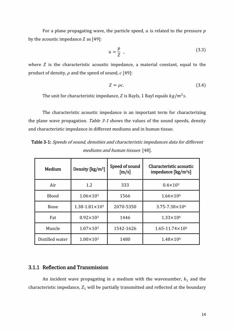
The characteristic acoustic impedance is an important term for characterizing

the plane wave propagation. Table 3-1 shows the values of the sound speeds, density

and characteristic impedance in different mediums and in human tissue.

Table 3-1: Speeds of sound, densities and characteristic impedances data for different

mediums and human tissues [48].

Medium Density [kg/m3] Speed of sound

[m/s] Characteristic acoustic

impedance [kg/m2s]

Air 1.2 333 0.4×103

Blood 1.06×103 1566 1.66×106

Bone 1.38-1.81×103 2070-5350 3.75-7.38×106

Fat 0.92×103 1446 1.33×106

Muscle 1.07×103 1542-1626 1.65-11.74×106

Distilled water 1.00×103 1480 1.48×106

3.1.1 Reflection and Transmission

An incident wave propagating in a medium with the wavenumber, 𝑘1 and the

characteristic impedance, 𝑍1 will be partially transmitted and reflected at the boundary

15

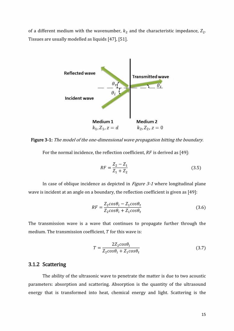
of a different medium with the wavenumber, 𝑘2 and the characteristic impedance, 𝑍2.

Tissues are usually modelled as liquids [47], [51].

Figure 3-1: The model of the one-dimensional wave propagation hitting the boundary.

For the normal incidence, the reflection coefficient, 𝑅𝐹 is derived as [49]:

𝑅𝐹 =𝑍2 − 𝑍1

𝑍1 + 𝑍2 (3.5)

In case of oblique incidence as depicted in Figure 3-1 where longitudinal plane

wave is incident at an angle on a boundary, the reflection coefficient is given as [49]:

𝑅𝐹 =𝑍2𝑐𝑜𝑠𝜃𝑖 − 𝑍1𝑐𝑜𝑠𝜃𝑡

𝑍2𝑐𝑜𝑠𝜃𝑖 + 𝑍1𝑐𝑜𝑠𝜃𝑡 (3.6)

The transmission wave is a wave that continues to propagate further through the

medium. The transmission coefficient, 𝑇 for this wave is:

𝑇 =2𝑍2𝑐𝑜𝑠𝜃𝑖

𝑍2𝑐𝑜𝑠𝜃𝑖 + 𝑍1𝑐𝑜𝑠𝜃𝑡 (3.7)

3.1.2 Scattering

The ability of the ultrasonic wave to penetrate the matter is due to two acoustic

parameters: absorption and scattering. Absorption is the quantity of the ultrasound

energy that is transformed into heat, chemical energy and light. Scattering is the

16

radiation of all, or part of the energy in an ultrasonic wave when incident on an obstacle.

The scattering can be in any direction. Reflection and refraction can be considered as

special cases of the scattering [51], [52].

Backscattering [52] is a reflection of the waves back to the direction from which

they were originated. Backscattering is useful for ultrasound imaging. Pulse echo

technique is used to detect the backscattered signal. Ultrasound transducers transmit a

pulse into a specimen to investigate, for example a heart. First, the transducer receives

the echo from the front face of the specimen and later from the back face. Other echoes

that are produced in between the two surfaces depend on the structural composition of

the tissue there.

The signal power, 𝑃𝑠 generated by one scatterer is characterized by the scattering

cross section which is a measure of the scattering magnitude and is derived as [48]:

𝑃𝑠 = 𝐼𝑖𝜎𝑠𝑐 , (3.8)

where 𝜎𝑠𝑐 is a scattering cross section and 𝐼𝑖 is a uniform intensity. The backscattering

cross section depends on the material type and denotes the strength of the material

scattering [48].

Provided that energy is scattered uniformly in all directions, the scattered

intensity,𝐼𝑠 is then given as [48]:

𝐼𝑠 =

𝑃𝑠

4𝜋𝑅2=

𝜎𝑠𝑐

4𝜋𝑅2𝐼𝑖 ,

(3.9)

where 𝑅is the distance to the scattering region. The received power,𝑃𝑟 with a

transducer radius, 𝑟 is then [48]:

𝑃𝑟 = 𝐼𝑠𝜋𝑟2 = 𝜎𝑠𝑐

𝑟2

4𝑅2𝐼𝑖 ,

(3.10)

Therefore, the received power depends on the scattering cross section, emitted

intensity, distance to the transducer and the size of the transducer aperture.

3.1.3 Attenuation

The ultrasound wave propagating in the tissue will experience energy loss or

attenuation due to absorption and scattering (reflection and refraction). Attenuation

17

can be expressed with exponential law as functions of distance. The amplitude loss

term, 𝐴(𝑧, 𝑡) can be added for single frequency plane wave propagation [53]:

𝐴(𝑧, 𝑡) = 𝐴0 exp(𝑖(𝜔𝑐𝑡 − 𝑘𝑧)) exp(−𝛼𝑧), (3.11)

where 𝜔𝑐 is the angular centre frequency and 𝛼 is the attenuation factor.

The amplitude attenuation coefficient, 𝛼 is the sum of the scattering and

absorption amplitude attenuation coefficients. The attenuation coefficient is expressed

in nepers per meters, but in medical ultrasound commonly given in decibel per

centimetre (dB/cm).

The attenuation that happens in tissue depends on the frequency. Attenuation

increases as frequency increases. The centre frequency, 𝑓0 of a transmitted signal will

be shifted down in frequency as the emitted pulse propagates through the tissue. The

shift in frequency of a Gaussian pulse is given as [48]:

𝑝(𝑡) = exp (−2(𝐵𝑟𝑓0𝜋)2𝑡2) cos(2𝜋𝑓0𝑡) (3.12)

where 𝐵𝑟 is a relative bandwidth and 𝑓0 is a centre frequency.

3.2 Ultrasound Transducers

Ultrasound transducers are widely used in diagnostic imaging systems.

Transducers come in a wide range of sizes and shapes and are often designed to operate

around specific centre frequencies. The piezoelectric transducer, depicted in Figure 3-2

is a single element transducer that consists of a piezoelectric plate, a mechanical

damping material, one or several matching layers and a casing. The ultrasound

transducer is connected to the medium by a physical contact. To increase the contact

between the transducer and the medium an ultrasound couplant can be used, e.g. a gel.

The piezoelectric plate is an important element in the transducer as this is where the

acoustical waves are generated and received. The ultrasound waves are generated by

the inverse piezoelectric effect, i.e. when the electric field is applied to the plate, the

plate responds to the corresponding stress field by contracting or expanding, depending

on the polarisation of the field [54]. In reception, when the ultrasound waves are

incident on the plate, the plate generates an electric potential in response to the applied

stress field. This is referred to as the piezoelectric effect. The choice of the dimensions of

the piezoelectric plate depends on the transducer’s application. The beam shape is to

18

large extent given by the ratio between the transducer diameter, 𝐷 relative to ultrasonic

wavelength, 𝜆. To achieve a directive beam, 𝐷 should be much larger than the

wavelength. This can be estimated from the opening angle in the far field, 𝜗0 = 𝜆/𝐷, for

example 𝐷 = 10𝜆 will give an opening angle of approximately 50. Aperture diameters

close to 𝜆, for example 0.7 𝜆 will lead to a much wider transmitted beam [54].

Figure 3-2: The schematic of the single element transducer [54].

The mechanical damping material is located behind the piezoelectric element

and is used to prevent excessive vibrations and to generate signals with shorter pulse

length that provides better spatial resolution in imaging. For a good damping, the

backing material should be matched with the piezoelectric acoustic impedance and have

high attenuation to eliminate reverberation within itself [54].

Often a large difference in the acoustical impedances of the media and the

piezoelectric material exist. For example, a common piezoceramic from Meggit

Ferroperm, Pz27 has an acoustical impedance of approximately 33 MRayl, whereas the

human body has an acoustical impedance of approximately 1.5 MRayl; a ratio of 22 [55].

A consequence of this is that most of the acoustical energy will be reflected at the

boundary between the piezoceramic and the human body. To reduce the reflection and

increase the transduction at the boundary between the transducer and the human body,

one or several matching layers are used. The matching layers form part of the

transducer construction and the impedance of the matching layer (for a transducer with

one matching layer) are chosen as the geometric mean between the impedance of the

19

piezoceramic and the media, and the thickness of the matching layer is chosen as one-

quarter of the wavelength in the matching layer. Matching a transducer to the medium

like this helps the ultrasonic waves to propagate efficiently into the object.

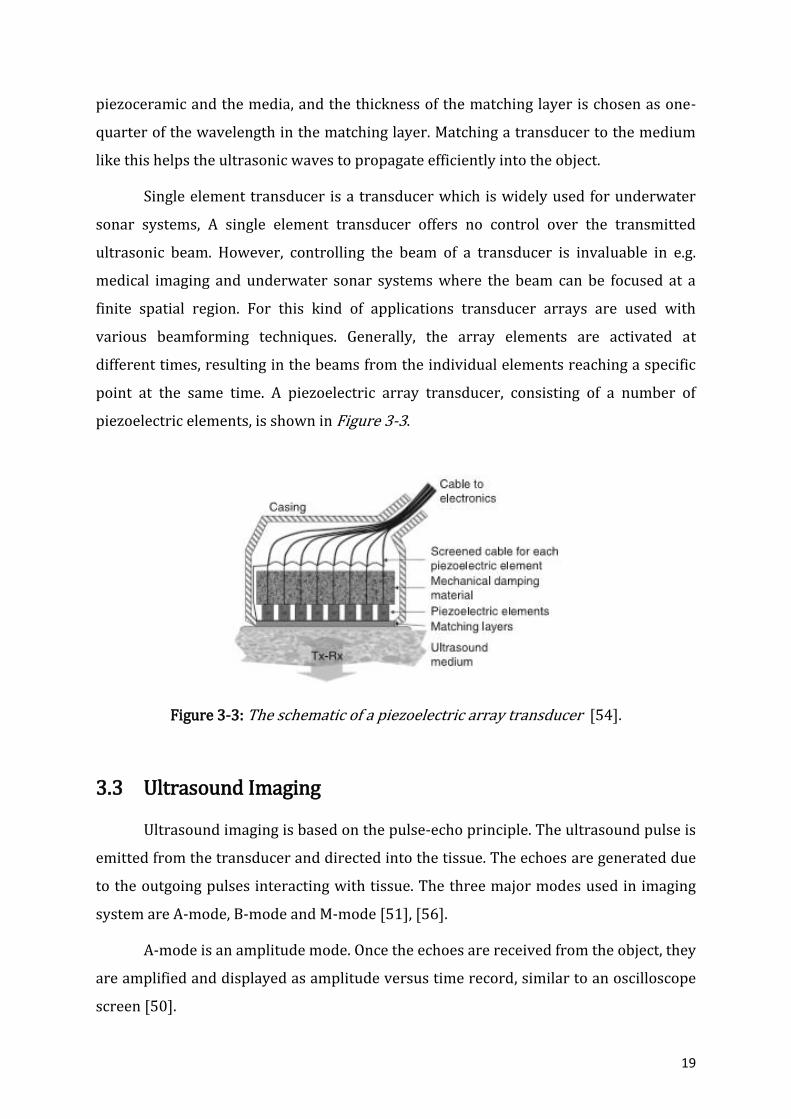
Single element transducer is a transducer which is widely used for underwater

sonar systems, A single element transducer offers no control over the transmitted

ultrasonic beam. However, controlling the beam of a transducer is invaluable in e.g.

medical imaging and underwater sonar systems where the beam can be focused at a

finite spatial region. For this kind of applications transducer arrays are used with

various beamforming techniques. Generally, the array elements are activated at

different times, resulting in the beams from the individual elements reaching a specific

point at the same time. A piezoelectric array transducer, consisting of a number of

piezoelectric elements, is shown in Figure 3-3.

Figure 3-3: The schematic of a piezoelectric array transducer [54].

3.3 Ultrasound Imaging

Ultrasound imaging is based on the pulse-echo principle. The ultrasound pulse is

emitted from the transducer and directed into the tissue. The echoes are generated due

to the outgoing pulses interacting with tissue. The three major modes used in imaging

system are A-mode, B-mode and M-mode [51], [56].

A-mode is an amplitude mode. Once the echoes are received from the object, they

are amplified and displayed as amplitude versus time record, similar to an oscilloscope

screen [50].

20

B-mode is known as a brightness mode. Brightness is proportional to the echo

amplitude. In a B-mode, the image is composed of many beams aimed in different

directions, creating a 2D image, typically in the 𝑧𝑥-plane, where 𝑧 refers to depth and x

to lateral direction. The brightness is related to the echo amplitude [51].

M-mode is a motion mode used to visualize time variation. The vertical 𝑧 axis is

depth downwards and horizontal 𝑡 axis is time. The images look similar to B-mode, but

the lateral dimension is time, creating 2D 𝑧𝑡-image. This mode is particular useful to

monitor heart motion and to receive an “image” of heart valves by observing distinct

patterns of heart along the time [56], [50].

3.4 Principles of Doppler Ultrasound

Doppler ultrasound is a non-invasive technique which is widely used to monitor

and measure the blood flow in the human body. It is sometimes difficult to visualize

blood circulation and Doppler ultrasound is a good solution to detect its movement in

the vessels. Doppler effect is also applied for heart valves imaging to track heart

contractions. It provides comprehensive information about fluid flow and heart

dynamics and abnormalities [50].

3.4.1 The Doppler Effect

The Doppler effect is a change in frequency as a sound source moves toward or

away from an observer. The Doppler frequency, 𝑓𝐷 or observed frequency for one-way

moving source is given as [57]:

𝑓𝐷 =

𝑓0

1 − (𝑐𝑠/𝑐0)𝑐𝑜𝑠𝜃,

(3.13)

where 𝑓0 is a transmitted frequency, 𝑐𝑠 is the velocity of the source, 𝑐0 is the speed of

sound and 𝜃 is an angle between the observer location and the source vector. From the

equation 3.13, Doppler-shifted frequency is then found as [57]:

∆𝑓 = 𝑓𝐷 − 𝑓0 = 𝑓0 (𝑐𝑠

𝑐0) 𝑐𝑜𝑠𝜃. (3.14)

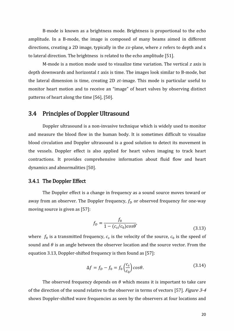
The observed frequency depends on 𝜃 which means it is important to take care

of the direction of the sound relative to the observer in terms of vectors [57]. Figure 3-4

shows Doppler-shifted wave frequencies as seen by the observers at four locations and

21

the angles relative to the direction of the source, where ∆𝑓 is a Doppler frequency and 𝑓𝑠

is a source frequency. Observers at B and D do not hear any Doppler shift.

Figure 3-4: Doppler frequencies seen by observers at different location and at the angles

relative to the direction of the source: (A) 0°, (B) 90°, (C) 270°, (D) 45° [57].

If the observer is moving and the source is stationary, then the formula for

Doppler-shifted frequency is [57]:

∆𝑓 = [1 + (𝑣𝑜𝑏𝑠/𝑐0)𝑐𝑜𝑠𝜃]𝑓0, (3.15)

where 𝑣𝑜𝑏𝑠 is the velocity of the observer. The Doppler-shifted frequency for the case

when both the source and the observer are moving turns to [57]:

∆𝑓 = 𝑓0[𝑐0 + 𝑐𝑜𝑏𝑠𝑐𝑜𝑠𝜃]/[𝑐0 − 𝑐𝑠𝑐𝑜𝑠𝜃], (3.16)

where 𝑐𝑠 is a velocity of the source.

3.4.2 Continuous-wave and Pulse-wave Doppler

In continuous-wave Doppler mode, the transducer is divided into halves where

one part continuously transmits and another part continuously receives signals [57].

This mode records the velocities of all moving targets in the ultrasound beam [58]. It

allows measurement of high velocities. In pulse-wave mode, transducer transmits and

then receives a signal after a pre-set time delay. One sample is acquired for each

transmitted pulse. The sampling area can be moved along the path of the ultrasound

beam for examination [58]. If the tissue is stationary then constant sampled values will

22

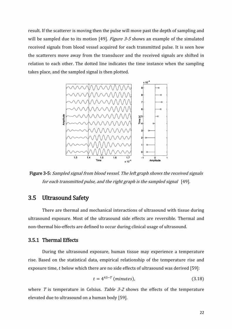
result. If the scatterer is moving then the pulse will move past the depth of sampling and

will be sampled due to its motion [49]. Figure 3-5 shows an example of the simulated

received signals from blood vessel acquired for each transmitted pulse. It is seen how

the scatterers move away from the transducer and the received signals are shifted in

relation to each other. The dotted line indicates the time instance when the sampling

takes place, and the sampled signal is then plotted.

Figure 3-5: Sampled signal from blood vessel. The left graph shows the received signals

for each transmitted pulse, and the right graph is the sampled signal [49].

3.5 Ultrasound Safety

There are thermal and mechanical interactions of ultrasound with tissue during

ultrasound exposure. Most of the ultrasound side effects are reversible. Thermal and

non-thermal bio-effects are defined to occur during clinical usage of ultrasound.

3.5.1 Thermal Effects

During the ultrasound exposure, human tissue may experience a temperature

rise. Based on the statistical data, empirical relationship of the temperature rise and

exposure time, 𝑡 below which there are no side effects of ultrasound was derived [59]:

𝑡 = 443−𝑇 (𝑚𝑖𝑛𝑢𝑡𝑒𝑠), (3.18)

where T is temperature in Celsius. Table 3-2 shows the effects of the temperature

elevated due to ultrasound on a human body [59].

23

Table 3-2: Temperature effects induced by ultrasound on a human body [59].

Temperature range [0C] Effect

37-39 No harm for extended exposure period

39-43 Adverse effect after long exposure time

>41 Threshold for fetal problems for long period

>41.8 Damage threshold

44-46 Protein coagulation

The fetus is considered as a sensitive biological site for long term ultrasound

exposure especially during the first trimester. If the transducer is placed directly on the

fetus skull, the elevated temperature of the bone may damage brain tissue. The

exposure of the ultrasound onto a fetus above 41 0C for 5 minutes or more should be

considered unsafe. According to a equation 3.18, the rise of temperature to 1.50C

corresponds to 158 minutes and a rise to 40C corresponds to 5 minutes provided that

transducer is located unmoved during the specified time [59].

3.5.2 Non-thermal Effects

Cavitation is a major type of the non-thermal effect of ultrasound [59]. Cavitation

is a collapsing of gas bubbles due to ultrasound exposure. This non-thermal effect of

ultrasound hardly occurs in human body naturally. For example, during imaging of the

fetus it does not show signs of any damage cases due to cavitation. Microbubbles that

are located in the intestine may cause small local damage. However, damages due to

cavitation are reversible and heal completely [59]. MI is a mechanical index used to

estimate a degree of the bio-effects due to cavitation that ultrasound may induce. MI is

defined as the maximum value of the peak negative pressure over the square root of the

centre frequency [60]. According to FDA, the ultrasound system is considered safe if MI

index does not exceed a maximum of 1.9 [61].

24

4 METHODOLOGY

Simulation is a method that extensively used in biomedical ultrasound. This

thesis uses computational model or computer based simulation to investigate the stated

problem. The simulation is based on the quantitative calculations and mathematical

model to determine numeric behaviour of the acoustic field in a test environment.

MATLAB R2016a version and Field II software programs were chosen to perform

simulations. Laboratory work was the second part of the research. Transmit/receive

hardware system and test environment were set up to couple a single-element

piezoelectric transducer. LABVIEW 2015 software was used to acquire and process the

signals from the hardware system that used to analyse the received signals from the test

environment.

There also were few discussions with the midwives in Horten Kommune

Helsestasjon who helped to understand the check-ups procedures for pregnant women

and available techniques. The continuous fetal heartbeat monitoring system as a

solution to a stillbirth reduction and fetal well-being monitoring was discussed with

them.

4.1 MATLAB and FIELD II Summary

Field II [62], [63], [64] is a simulation program for ultrasound systems which can

be interfaced with MATLAB. It uses the spatial impulse concept based on Tupholme-

Stepanishen method. The field of any kind of excitation is found by the convolution of

the spatial impulse response and excitation function. The excitation pulse is a voltage

applied to the transducer terminals. The impulse response is called spatial impulse

response since it varies as a function of the position relative to the transducer.

Field II allows the simulations of any kind of transducer geometries and

excitation. Pulsed-wave and continuous-wave fields can be calculated for transmit and

pulse-echo. Apodization and various focusing schemes can be utilized though

introduced time lines. The main application of Field II is to simulate an image. It is also

applied for the simulation of the velocity measurements with ultrasound using Doppler

effect. It is mostly applied for the measurement of the blood flow in the vessels.

25

There are some approximations made in Field II:

Spatial impulse response assumes linear propagation;

Transducer surface is divided into smaller squares, called ‘mathematical

elements’ to imitate piston vibrations. The edges in piston may vibrate less than

the centre. The responses from each of the squares are then summed up to

produce a response;

The sound field from each mathematical element is calculated using the far field

approximation for the element to make calculation fast. The sound field from the

whole aperture is found by summing the contributions from the mathematical

elements. These results will be valid also in the near field of the whole aperture.

Point scatterer approach is used to construct a phantom. The ultrasound image

consists of a clutter and larger tissue structures. Clutter is a noise artifact in ultrasound

images that obscures the image target and complicates anatomical measurements [65].

The image is then built from the collection of the randomly placed point scatterers with

Gaussian amplitude. The relative amplitude between the different types of scatterers is

scaled to generate clutter and larger structures [66]. The fully developed realistic image

should have at least 10 randomly generated scatterers per resolution cell. Usually,

200 000 to 1 million scatterers are generated to yield a normal ultrasound image.

The received signals from the point scatterers are then calculated for each line in

the image defined by focusing scheme. The resulted RF signal is then found by the

summing the received signals from the scatterers. RF signal is an adopted term from the

communication engineering field and it states for “radio frequency”. This term is

accepted and used in ultrasound field. The received RF signal is a voltage output signal

of the beamformer [67].

It is possible to simulate a Doppler ultrasound scanning in Field II. The Doppler

frequency shift can be determined through the estimation of the time difference

between the successive snap shots of images. Different images are created with changed

positions or amplitudes of the scatterers to imitate movements of the tissue structure.

The received signals from moving scatterers are then analyzed and frequency shifts are

extracted.

26

4.2 Fetus and Pregnant Woman Design Parameters

It is important to investigate the anatomy of the abdomen of the pregnant

woman for the transducer to be attached. The third trimester of gestation is chosen for

the study with a woman having one fetus. During the third trimester, the baby does not

make big movements and eventually stays at one position with a head down [68]. The

abdomen of a pregnant woman consists of the abdominal wall, uterine wall and

amniotic fluid surrounding a fetus [68], as depicted in Figure 4-1. Since baby is big

enough to occupy uterus during the most of the third trimester period, the thickness of

the amniotic fluid is neglected for the simulations.

Figure 4-1: Anatomy of the woman in the third trimester of gestation.

Uterine wall consists of three layers such as endometrium, myometrium and

perimetrium. Myometrium is the major constituent of the uterine wall [69]. The

abdominal wall consists of a subcutaneous tissue, muscle and skin [70], [71].

It is important to define woman weight which will be considered for the study.

The weight of the woman affects the thickness of the abdominal and uterine walls.

These thicknesses will define the distance of the transducer to a fetal heart. Table 4-1

shows the parameters used to perform simulation which were taken from the studies

[69], [72].

27

Table 4-1: Woman size parameters.

Variable Range

Maternal age [years] 21-44

Maternal weight [kg] 42-110

Mean, (range)

Abdominal wall depth [mm] 38, (9-92)

Uterine wall depth (myometrial thickness) [mm] 9.05, (-)

Abdominal wall depth is measured from the abdominal wall surface to the

anterior wall of the amniotic sac. Posterior uterine wall depth is defined as the distance

from the abdominal wall surface to the posterior uterine wall surface. Figure 4-2 shows

the schematics of the woman abdomen.

Figure 4-2: Schematic drawing of the woman abdomen, 1 – abdominal wall depth, 2 -

uterine wall thickness, 3 – posterior uterine wall depth.

Posterior uterine wall depth was calculated from the symphysis-fundal height

(SFH) measurements. For simplicity of calculations, it was assumed that uterine has a

circular shape. SFH is a height of the uterus which changes according to a gestation age

[73], depicted in Figure 4-3. It is measured from the top of the uterus to the pubic bone

as shown in Figure 4-4.

28

Figure 4-3: SFH measurements versus gestational age, provided by midwives from

Horten kommune helsetjenesten for barn og unge.

SFH is approximated to behave as a circumference of a circle, 𝐶 and it equals to:

𝐶 = 2𝑆𝐹𝐻, (4.1)

and posterior uterine wall depth, 𝐷 is then derived as:

𝐷 =

2𝑆𝐹𝐻

𝜋,

(4.2)

Table 4-2 shows SFH measurements extracted from the Figure 4-3 and

calculated posterior uterine all depth for the third gestation trimester.

Table 4-2: Posterior uterine wall depth and SFH change according to a gestation age.

Gestation age [weeks] SFH [cm] D [cm]

28-31 26.0-28.5 16.6-18.1

32-35 29.5-32.0 18.9-20.4

36-40 32.5-34.5 20.7-22.0

29

Figure 4-4: Schematic of SFH measurement procedure.

The heart wall consists of the three major layers such as endocardium,

myocardium and epicardium surrounded by pericardium sac. The total thickness of

these layers is around 1-2 mm for a fetal heart [74], [75]. The heart sizes change during

the gestational age progression. Table 4-3 shows the cardiac sizes for the third

trimester which are assumed for the simulation.

Table 4-3: Cardiac sizes for the third trimester [76], [77].

Gestation age [weeks] Cardiac circumference [mm] Cardiac radius [mm]

28-31 114-129 18-20

32-35 134-148 21-23

36-40 152-169 24-26

4.3 Simulation Design

4.3.1 Ultrasound Transducer Design Model

Single-element piston transducer is used to perform simulations in Field II for

Doppler ultrasound. The circular plate disk is divided into mathematical elements, as

30

shown in Figure 4-5. The size of each element is 1 mm. The transducer is always

positioned at (0, 0, 0) coordinates.

Figure 4-5: Piston transducer divided into 1mm mathematical elements.

Transducer aperture radius is the design parameter for the transducer that will

be varied for simulations to investigate the problem. Table 4-4 summarizes the design

parameters used during the simulations.

Table 4-4: Transducer design parameters.

Parameters Value

Central frequency 2.0 MHz

Transducer radius 5 mm

2 mm

4.3.2 Heart Model

Ultrasound image and schematic of the fetal heart are shown in Figure 4-6. Based

on these images, the fetal heart is assumed to have a circular shape for 2-D B-mode

image construction in Field II.

31

Figure 4-6: Ultrasound image of the fetal heart (right) and its schematics with identified

heart constituents: LV (left ventricle), RV (right ventricle), ventricular septum,

moderator band, pulmonary veins, atrial septum and crux [78].

The heart model consists of the heart with a heart wall filled with blood and a

surrounding tissue. Two radii, 𝑟1 and 𝑟2 are introduced to define the thickness of the

heart wall. Figure 4-7 illustrates a proposed heart model. Heart phantom is then

constructed by the generation of random point scatterers and deterministic scaled

amplitudes. The point scatterers are given the amplitude properties of tissue or blood.

The blood cells are mainly responsible for the scattering when ultrasound interacts with

blood. Scattering is very weak from the blood cells since blood cells have very small

micrometre sizes as compared to a heart wall muscle tissue. Therefore, it is assumed

that the amplitude of point scatterers inside the heart is zero. Heart tissue is a highly

scattered region and its amplitude is set to 10. The background tissue is responsible to

simulate the realistic surrounding environment around the fetal heart. The number of

background point scatterers is a varied parameter to simulate different background

conditions. Increasing the amplitude and number of scatterers will increase their

scattering properties which will make difficult to distinguish the heart wall boundaries

in a “noisy” environment.

32

Figure 4-7: Heart model for Field II simulation, r1 and r2 are heart wall radii.

Table 4-5 summarizes the amplitude properties of the point scatterers for blood,

heart muscle and background tissue used for simulation.

Table 4-5: Amplitude scaling factors for blood, heart wall and surrounding tissue.

Objects Amplitude scaling factor

Blood 0

Heart wall 10

Surrounding tissue 1

The simulated B-mode images of the heart were received in Field II. B-mode

images were simulated with linear array transducer with 192 elements. These images

are used to view the heart phantom and its position relative to the transducer surface.

Number of scatterers was varied to receive different granular textures. Table 4-6

summarizes the number of simulations performed for this part.

33

Table 4-6: Simulation of the heart phantom with varied number of scatterers.

Simulation No. Number of point scatterers

1 1 000

2 10 000

3 200 000

4 1 000 000

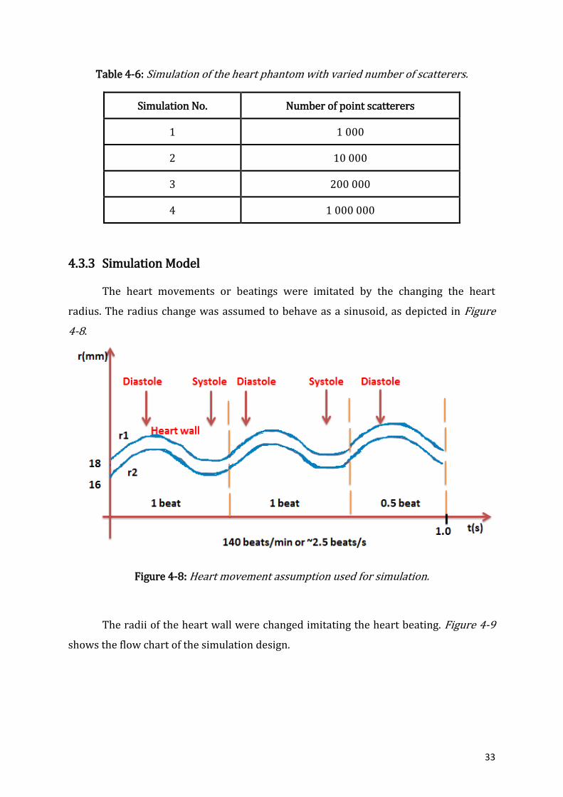
4.3.3 Simulation Model

The heart movements or beatings were imitated by the changing the heart

radius. The radius change was assumed to behave as a sinusoid, as depicted in Figure

4-8.

Figure 4-8: Heart movement assumption used for simulation.

The radii of the heart wall were changed imitating the heart beating. Figure 4-9

shows the flow chart of the simulation design.

34

Figure 4-9: The flow chart of the simulation model, where r1 and r2 are the heart wall

radii, R is a radius of the transducer aperture, f0 is the central frequency.

The received signal is recorded once the heart wall radii change. One cardiac

cycle was simulated. RF signals are analytically analysed after they were recorded. The

simulation is divided into four case studies which are case study A, B, C and D. Case

study A is a case where the heart phantom is a highly scattered region and the

background tissue is a weakly scattered region. In case study B, the surrounding tissue

is now highly scattered region and heart is a weak scattered region. Case studies C and

D analyse the situation when the heart position due to baby movements or transducer

location can be displaced. The heart position is slightly shifted in x-direction in Case

study C. The phantom is then shifted in z-direction in case study D. The design

parameters are further specified in below subsections.

35

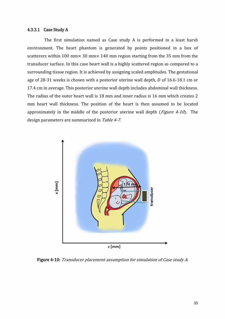
4.3.3.1 Case Study A

The first simulation named as Case study A is performed in a least harsh

environment. The heart phantom is generated by points positioned in a box of

scatterers within 100 mm× 30 mm× 140 mm region starting from the 35 mm from the

transducer surface. In this case heart wall is a highly scattered region as compared to a

surrounding tissue region. It is achieved by assigning scaled amplitudes. The gestational

age of 28-31 weeks is chosen with a posterior uterine wall depth, 𝐷 of 16.6-18.1 cm or

17.4 cm in average. This posterior uterine wall depth includes abdominal wall thickness.

The radius of the outer heart wall is 18 mm and inner radius is 16 mm which creates 2

mm heart wall thickness. The position of the heart is then assumed to be located

approximately in the middle of the posterior uterine wall depth (Figure 4-10). The

design parameters are summarized in Table 4-7.

Figure 4-10: Transducer placement assumption for simulation of Case study A.

36

Table 4-7: Simulation design parameters for Case study A.

Fetus and woman

Gestational age [weeks]

Outer heart radius [mm]

Transducer-heart distance [mm]

28-31 18 87

Transducer

Centre frequency, 𝒇𝟎 [MHz]

Aperture radius [mm]

-

2 5 -

Phantom Heart amplitude Blood amplitude Background amplitude

10 0 1

One cardiac cycle which includes systole and diastole is simulated with a heart

rate of 140 bpm or 2.33 Hz of the heart frequency.

4.3.3.2 Case Study B

The design parameters used in the case study B are shown in Table 4-8. In this

study, heart muscle is a weakly scattered region and background tissue is a highly

scattered region. The amplitude of the heart muscle is now scaled to 1, and the

amplitude of the background is scaled to 10. Other design parameters remain

unchanged from the case study A.

Table 4-8: Design parameters.

Fetus and woman

Gestational age (weeks)

Heart radius [mm] Transducer-heart distance [mm]

28-31 18 87

Transducer

Centre frequency, 𝒇𝟎 [MHz]

Aperture radius [mm]

-

2 5 -

Phantom Heart amplitude Blood amplitude Background

amplitude

1 0 10

37

4.3.3.3 Case Study C

The heart centre position is slightly moved in x-direction. The previous centre

of the heart (𝑥𝑐 , 𝑧𝑐) was (0, 70). The changed position in this case is (10, 70). The

scatterer box is widened and it has dimensions of 140 mm× 30 mm× 140 mm. The

design parameters are summarized in Table 4-9.

Table 4-9: Design parameters for case study C.

Fetus and woman

Gestational age (weeks)

Heart radius [mm] Transducer-heart

distance [mm]

28-31 18 87

Transducer

Centre frequency, 𝒇𝟎 [MHz]

Aperture radius [mm]

2 5 2

Phantom Heart amplitude Blood amplitude Background amplitude

1 0 10

Figure 4-11: Possible movements of the transducer and a fetus assumed in simulation

for case study C and D.

38

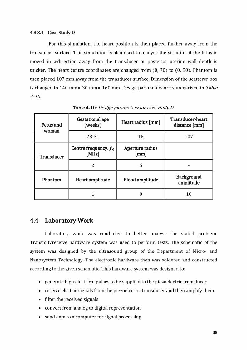
4.3.3.4 Case Study D

For this simulation, the heart position is then placed further away from the

transducer surface. This simulation is also used to analyse the situation if the fetus is

moved in z-direction away from the transducer or posterior uterine wall depth is

thicker. The heart centre coordinates are changed from (0, 70) to (0, 90). Phantom is

then placed 107 mm away from the transducer surface. Dimension of the scatterer box

is changed to 140 mm× 30 mm× 160 mm. Design parameters are summarized in Table

4-10.

Table 4-10: Design parameters for case study D.

Fetus and woman

Gestational age (weeks)

Heart radius [mm] Transducer-heart

distance [mm]

28-31 18 107

Transducer

Centre frequency, 𝒇𝟎 [MHz]

Aperture radius [mm]

2 5 -

Phantom Heart amplitude Blood amplitude Background amplitude

1 0 10

4.4 Laboratory Work

Laboratory work was conducted to better analyse the stated problem.

Transmit/receive hardware system was used to perform tests. The schematic of the

system was designed by the ultrasound group of the Department of Micro- and

Nanosystem Technology. The electronic hardware then was soldered and constructed

according to the given schematic. This hardware system was designed to:

generate high electrical pulses to be supplied to the piezoelectric transducer

receive electric signals from the piezoelectric transducer and then amplify them

filter the received signals

convert from analog to digital representation

send data to a computer for signal processing

39

More detailed explanation of the system performance can be obtained from the

ultrasound group in the Department of Micro- and Nanosystem Technology.

LabVIEW 2015 is a system-design platform utilizes the graphical language. It was

used to acquire and process the signals received from the transmit/receive hardware

system. The LabVIEW template to drive the hardware system was supplied by the

ultrasound group. The code for the “Process” state was only implemented for required

application which is to compute the phase shifts between the received signals.

40

5 RESULTS

5.1 B-mode Heart Image

B-mode images were simulated with varied number of randomly generated point

scatterers (Figure 5-1). This allows modelling a speckle. Speckle is a grainy texture

arises from the constructive and destructive interference of these scatterers [79]. The

simulated phantom can be used for Doppler shift simulations.

Figure 5-1: B-mode images of the phantom with varied number of scatterers (N): (a)

N=1000, (b) N=10 000, (c) 200 000 and (d) N=1 000 000.

41

B-mode image with number of scatterers N=200 000 and 1 000 000 are

statistically equal. It was required 18 hours to build the heart phantom with one million

scatterers as compared to the image with 200 000 scatterers which took 4 hours. B-

mode image with N equal to 200 000 is fully developed speckle and these number of

scatterers will be used to construct phantom for Doppler ultrasound.

5.2 Case Studies

Theoretical analysis is needed in order to analyse the received RF signals.

Doppler frequency shift is generated by cardiac motion. The velocity of the heart

depends on a time instance when it is recorded since heart experiences accelerations

and decelerations (Figure 5-2). The displacement of the heart during the cardiac cycle is

considered to be a sinusoid:

𝑟(𝑡) = 18 + sin(2𝜋𝑓ℎ𝑡), (5.1)

where 𝑓ℎ is a frequency of the heartbeat. The velocity is found as a derivative of the

radius change over time the heart beats:

𝑣 =

𝑑𝑟(𝑡)

𝑑𝑡=

𝑑

𝑑𝑡(18 + sin(2𝜋𝑓ℎ𝑡)) = 2𝜋𝑓ℎcos (2𝜋𝑓ℎ𝑡)

(5.2)

Figure 5-2: The velocity of the heart movement for one cardiac cycle.

The maximum velocity, 𝑣𝑚𝑎𝑥 of the heart motion is achieved when cos(2𝜋𝑓ℎ𝑡) =

1 and it equals to:

𝑣𝑚𝑎𝑥 = 2𝜋𝑓ℎ (5.3)

42

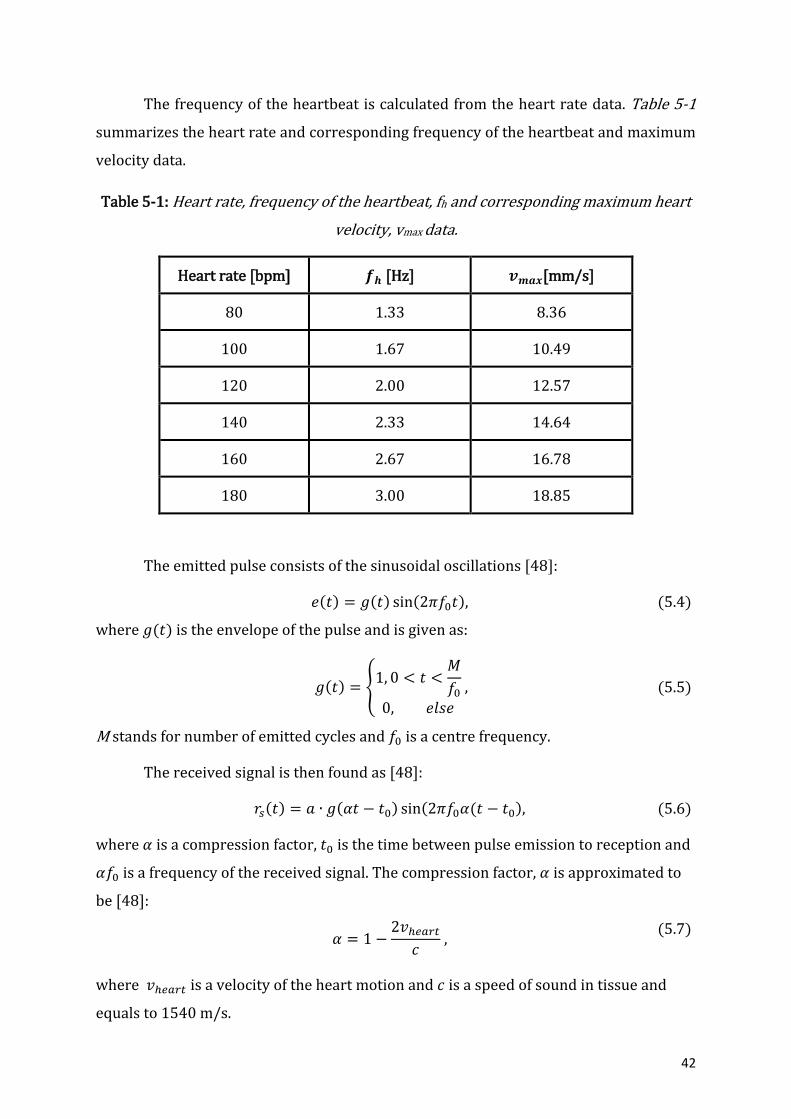
The frequency of the heartbeat is calculated from the heart rate data. Table 5-1

summarizes the heart rate and corresponding frequency of the heartbeat and maximum

velocity data.

Table 5-1: Heart rate, frequency of the heartbeat, fh and corresponding maximum heart

velocity, vmax data.

Heart rate [bpm] 𝒇𝒉 [Hz] 𝒗𝒎𝒂𝒙[mm/s]

80 1.33 8.36

100 1.67 10.49

120 2.00 12.57

140 2.33 14.64

160 2.67 16.78

180 3.00 18.85

The emitted pulse consists of the sinusoidal oscillations [48]:

𝑒(𝑡) = 𝑔(𝑡) sin(2𝜋𝑓0𝑡), (5.4)

where 𝑔(𝑡) is the envelope of the pulse and is given as:

𝑔(𝑡) = {

1, 0 < 𝑡 <𝑀

𝑓0

0, 𝑒𝑙𝑠𝑒

, (5.5)

M stands for number of emitted cycles and 𝑓0 is a centre frequency.

The received signal is then found as [48]:

𝑟𝑠(𝑡) = 𝑎 ∙ 𝑔(𝛼𝑡 − 𝑡0) sin(2𝜋𝑓0𝛼(𝑡 − 𝑡0), (5.6)

where 𝛼 is a compression factor, 𝑡0 is the time between pulse emission to reception and

𝛼𝑓0 is a frequency of the received signal. The compression factor, 𝛼 is approximated to

be [48]:

𝛼 = 1 −

2𝑣ℎ𝑒𝑎𝑟𝑡

𝑐 ,

(5.7)

where 𝑣ℎ𝑒𝑎𝑟𝑡 is a velocity of the heart motion and 𝑐 is a speed of sound in tissue and

equals to 1540 m/s.

43

The Doppler frequency, 𝑓𝑑 is the difference of the transmitted and received

frequency and found as [57]:

𝑓𝑑 = 𝛼𝑓0 − 𝑓0 = (𝛼 − 1)𝑓0 = −

2|𝑣ℎ𝑒𝑎𝑟𝑡|𝑐𝑜𝑠𝜃

𝑐𝑓0,

(5.8)

where 𝜃 is an angle between the ultrasound beam and the velocity vector.

Assuming that the velocity vector and ultrasound beam are at 00 lead to 𝑐𝑜𝑠𝜃 =

1. The Doppler frequencies for heartbeat frequencies of 1.67, 2.33 and 3 Hz are

calculated for the centre frequency of 2 MHz, as shown in Table 5-2.

Table 5-2: Calculated Doppler frequencies for 2 MHz centre frequency.

Centre frequency, 𝒇𝟎 [MHz] 𝒇𝒉 [Hz] 𝒗𝒎𝒂𝒙[mm/s] 𝒇𝒅 [Hz]

2.00

1.67 10.49 -27.24

2.33 14.64 -38.03

3.00 18.85 -48.96

The task of true and simulated Doppler instrument is to be able to detect such

small frequency shifts. It is mostly impossible to detect small shifts with pulsed Doppler

since the downshift in frequency due to attenuation will dominate over the Doppler

frequency shift. Another method to analyse the Doppler system is a computation of the

time shifts between the consecutive received pulses. Two consecutive received signals

are compared. The time between the transmit pulses is 𝑇𝑃𝑅𝐹. The movement of the heart

scatterers will yield a small displacement in their positions which can be countered as a

shift in time relative to the pulse shift. The second received signal (𝑟𝑠2) will be shifted in

time as compare to the first received signals (𝑟𝑠1) as [48]:

𝑟𝑠2 = 𝑟𝑠1(𝑡 − 𝑡𝑠) , (5.9)

where 𝑡𝑠 is a time shift. The velocity can be estimated by measuring the distance

travelled during a certain time interval. The mean velocity is then the distance travelled

divided by the time. The time displacement or time shift, 𝑡𝑠 between the successive

received signals is [57]:

𝑡𝑠 =

2∆𝑧

𝑐=

2𝑇𝑃𝑅𝐹𝑣ℎ𝑒𝑎𝑟𝑡𝑐𝑜𝑠𝜃

𝑐 ,

(5.10)

44

where ∆𝑧 is an imaging depth. Therefore, the time shift is proportional to the velocity of

the heart movement. The equation 5.10 can be rewritten as:

𝑡𝑠 = 𝐴𝑣ℎ𝑒𝑎𝑟𝑡, (5.11)

where A is then a constant and equals to:

𝐴 =

2𝑇𝑃𝑅𝐹𝑐𝑜𝑠𝜃

𝑐 .

(5.12)

Therefore instead of measurement of the frequency shifts, phase shift

measurement can be employed by estimating the time delay of the received signals due

to the displacement of the scatterers.

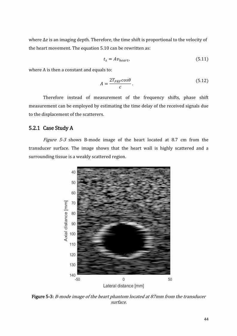
5.2.1 Case Study A

Figure 5-3 shows B-mode image of the heart located at 8.7 cm from the

transducer surface. The image shows that the heart wall is highly scattered and a

surrounding tissue is a weakly scattered region.

Figure 5-3: B-mode image of the heart phantom located at 87mm from the transducer surface.

45

The beam profile and heart position in the pressure field can be seen in the

Figure 5-4 with a piston transducer having 5 mm aperture.

Figure 5-4: Beam profile for a round flat aperture with 5 mm radius with a heart position in the pressure field for case study A.

The time, 𝑡𝑑 for the first transmitted and received signal by a transducer should be:

𝑡𝑑 =

2∆𝑧

𝑐=

2(87𝑚𝑚)

1540𝑚/𝑠= 1.13 × 10−4𝑠.

First, signals were received from the stationary structure when the radius of the

heart does not change. Figure 5-5 shows the summed RF signals and Figure 5-6 shows

individual RF lines for each transmitted pulses. Delay time, 𝑡𝑑 for the first received

signal is found from the Figure 5-5 and it is equal to 1.217× 10−4𝑠 which is slightly

different from the computed value. Transmitted pulse is reflected from the front and

back wall of the heart, as seen in Figure 5-5. The amplitudes of the received signals are

much lower for the back heart wall as compared to the amplitudes of the received

signals from the front heart wall. The reason for it may be the position of the back heart

wall which is located in a pressure field with a lower intensity. The blood region is

observed where no RF lines are received. There are no time shifts observed between the

received signals since the phantom is stationary (Figure 5-6).

46

Figure 5-5: RF data received by a transducer.

Figure 5-6: Individual RF lines for non-moving heart wall.

Blood region

Front heart wall

Back heart wall

47

RF data were received when radii of the heart changed imitating a heartbeat for

one cardiac cycle. Figure 5-7 shows the heart wall radii change. The phase shifts

between consecutive received signals were calculated and analysed (Table 5-3). Figure

5-9 illustrates the received signals due to a number of pulse emissions. The received

signals are shown on top of each other. The phase shifts with respect to the red line in

the figure are extracted. Velocity of the heart scatterers were calculated using equation

5.10 and assuming that the velocity vector and ultrasound beam are at 00.

Figure 5-7: The change of the heart radii over one cardiac cycle.

Figure 5-8: Summed received signals from the heart phantom for case study A.

𝑡0

𝑡2 𝑡1

𝑡3 𝑡4

𝑡5

𝑡6 𝑡7 𝑡8

𝑡9 𝑡10

Blood region

Front heart wall

Back heart wall

48

Figure 5-9: Received signals for each RF line.

Table 5-3: Time shifts between consecutive signals and measured velocity of the heart

scatterers for case study A.

Time shift, 𝒕𝒔

Time shift, 𝒕𝒔 [× 𝟏𝟎−𝟔s]

Measured velocity of heart scatterers, 𝒗𝒉𝒆𝒂𝒓𝒕,𝒎 [mm/s]

𝑡0 − 𝑡1 0.8 14.54

𝑡1 − 𝑡2 0.5 8.95

𝑡2 − 𝑡3 0.0 0.00

𝑡3 − 𝑡4 -0.2 -3.58

𝑡4 − 𝑡5 -0.8 -14.32

𝑡5 − 𝑡6 -0.4 -7.16

𝑡6 − 𝑡7 -0.8 -14.32

𝑡7 − 𝑡8 0.0 0.00

𝑡8 − 𝑡9 0.8 14.32

𝑡9 − 𝑡10 0.4 7.16

Front heart wall Blood Back heart wall

49

Figure 5-10 illustrates the resulting sampled signal which is the time shifts

between the received signals for 11 transmitted pulses. The time shift is proportional to

the velocity of the heart movement. The constant sampled values will result if the heart

is stationary. The changing values are measured when heart beats as shown in the

Figure 5-10.

The measured velocities from the time shifts are compared with actual velocities

of the heart scatterers, as shown in Figure 5-11.

Figure 5-10: Sampled signal. Time shifts between the received signals for 11 transmitted

pulses. Case study A.

Figure 5-11: Graph of the measured and actual velocities of the heart scatterers for case study A.

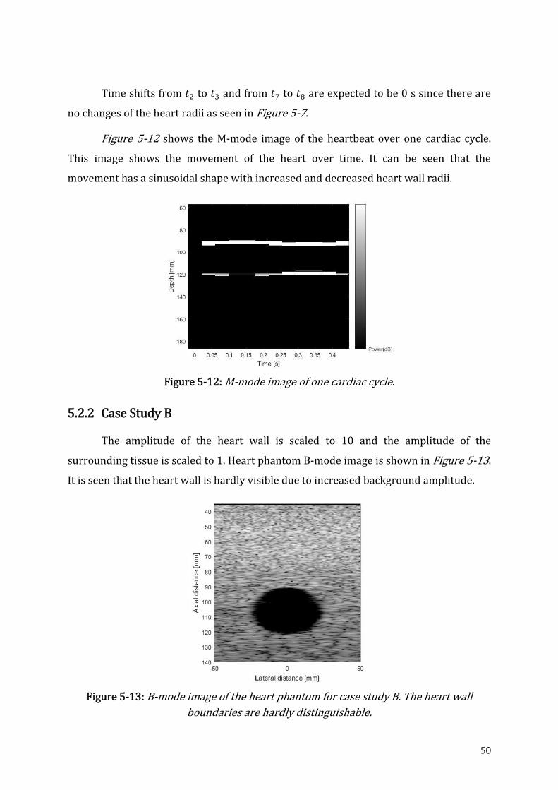
50

Time shifts from 𝑡2 to 𝑡3 and from 𝑡7 to 𝑡8 are expected to be 0 s since there are

no changes of the heart radii as seen in Figure 5-7.

Figure 5-12 shows the M-mode image of the heartbeat over one cardiac cycle.

This image shows the movement of the heart over time. It can be seen that the

movement has a sinusoidal shape with increased and decreased heart wall radii.

Figure 5-12: M-mode image of one cardiac cycle.

5.2.2 Case Study B

The amplitude of the heart wall is scaled to 10 and the amplitude of the

surrounding tissue is scaled to 1. Heart phantom B-mode image is shown in Figure 5-13.

It is seen that the heart wall is hardly visible due to increased background amplitude.

Figure 5-13: B-mode image of the heart phantom for case study B. The heart wall

boundaries are hardly distinguishable.

51

Figure 5-14 shows the summed received RF signals for 11 transmit pulses. There

are additional signals present as compared with the summed received signals in case

study A. These extra signals should come from the highly scattered surrounding

background tissue. Figure 5-15 illustrates individual RF lines for each transmit pulse.

Received signals from background tissue, front and back heart walls and blood can be

visualized in the figure.

Figure 5-14: Summed received RF lines for case study B.

Figure 5-15: Received signals for 11 transmit pulses for case study B. The point indicates

the maximum amplitude found in overall received signals.

Blood region

Front heart wall

Back heart wall

Background Front heart wall Blood Back heart wall Background

52

Table 5-4 shows the time shifts between the received RF lines. Figure 5-15 is

used to calculate time shifts between the consecutive received RF lines.

Table 5-4: Time shift calculation between consecutive received RF lines and measured

velocities of the heart scatterers. Case study B.

Time

shift, 𝒕𝒔

Time shift,

𝒕𝒔[× 𝟏𝟎−𝟔s]

Measured velocity of heart scatterers,

𝒗𝒉𝒆𝒂𝒓𝒕,𝒎 [mm/s]

𝑡0 − 𝑡1 0.5 8.95

𝑡1 − 𝑡2 0.5 8.95

𝑡2 − 𝑡3 0.0 0.00

𝑡3 − 𝑡4 -1.0 -17.91

𝑡4 − 𝑡5 -0.4 -7.16

𝑡5 − 𝑡6 -0.6 -10.74

𝑡6 − 𝑡7 -0.7 -12.53

𝑡7 − 𝑡8 0.0 0.00

𝑡8 − 𝑡9 1.1 19.70

𝑡9 − 𝑡10 0.7 12.53

Time shifts from 𝑡2 to 𝑡3 and from 𝑡7 to 𝑡8 equal to 0 s since there is no change of

radius of the heart wall. The velocity was found using the equation 5.10 with 𝜃 = 00

which is an angle between the transducer probe and velocity vector. Figure 5-16

illustrates the sampled signal plot. The plot shows times shifts between the successive

received signals for 11 transmit pulses.

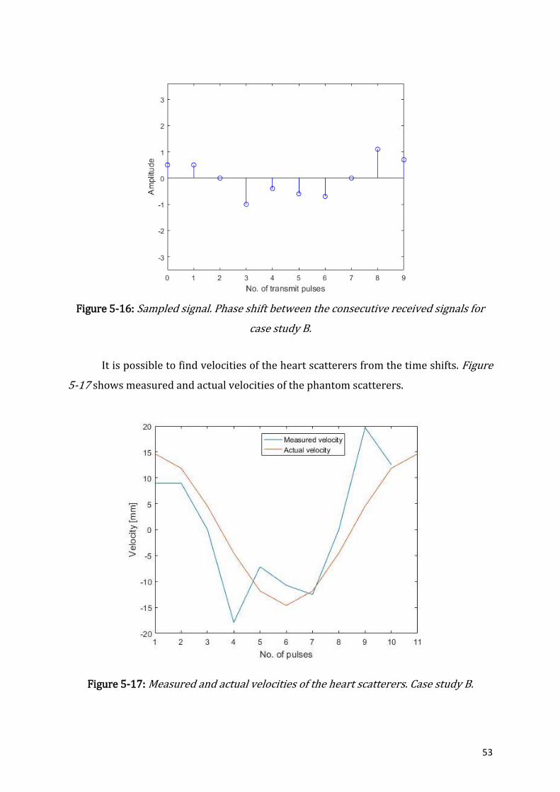
53

Figure 5-16: Sampled signal. Phase shift between the consecutive received signals for

case study B.

It is possible to find velocities of the heart scatterers from the time shifts. Figure

5-17 shows measured and actual velocities of the phantom scatterers.

Figure 5-17: Measured and actual velocities of the heart scatterers. Case study B.

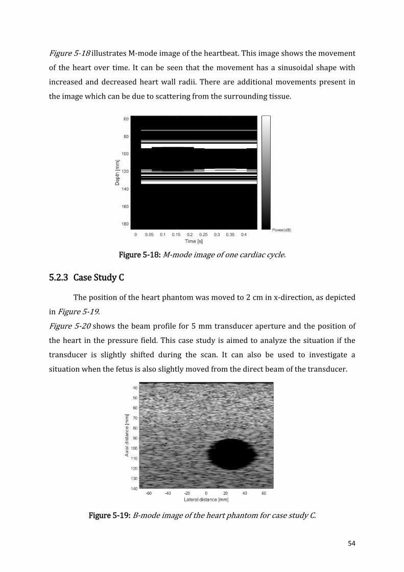
54

Figure 5-18 illustrates M-mode image of the heartbeat. This image shows the movement

of the heart over time. It can be seen that the movement has a sinusoidal shape with

increased and decreased heart wall radii. There are additional movements present in

the image which can be due to scattering from the surrounding tissue.

Figure 5-18: M-mode image of one cardiac cycle.

5.2.3 Case Study C

The position of the heart phantom was moved to 2 cm in x-direction, as depicted

in Figure 5-19.

Figure 5-20 shows the beam profile for 5 mm transducer aperture and the position of

the heart in the pressure field. This case study is aimed to analyze the situation if the

transducer is slightly shifted during the scan. It can also be used to investigate a

situation when the fetus is also slightly moved from the direct beam of the transducer.

Figure 5-19: B-mode image of the heart phantom for case study C.

55

Figure 5-20: Beam profile of the 5 mm transducer aperture and position of the heart in

the pressure field. Case study C.

5.2.3.1 Aperture Radius 5 mm

The heart position is moved to 2 cm away from the transducer central beam.

The radius of the transducer aperture is 5 mm. Figure 5-21 and Figure 5-22 depict

received RF lines. The received signals from the back heart wall are weak. The time

shifts from the front heart wall received signals are calculated using Figure 5-22.

Figure 5-21: Received RF lines for 11 transmit pulses for case study C with a transducer aperture of 5 mm.

Blood region

Front heart wall

Back heart wall

56

Figure 5-22: Individual RF lines for 11 transmit pulses. Case study C.

Table 5-5 shows calculated time shifts between the successive received signals

and measured velocity. The velocity was found using the equation 5.10 with 𝜃 = 00

which is an angle between the transducer probe and velocity vector. The blood region is

reduced as seen in Figure 5-21. The reason may be due to the position of the heart

which is not directly located in the central lobe of the pressure field.

Table 5-5: Time shifts calculation between consecutive received RF lines. Case study C.

Time shift, 𝒕𝒔

Time shift, 𝒕𝒔[× 𝟏𝟎−𝟔s]

Velocity of heart scatterers, 𝒗𝒉𝒆𝒂𝒓𝒕 [mm/s]

𝑡0 − 𝑡1 1.0 17.91

𝑡1 − 𝑡2 0.6 10.74

𝑡2 − 𝑡3 0.0 0.00

𝑡3 − 𝑡4 -0.6 -10.74

𝑡4 − 𝑡5 -0.9 -16.12

𝑡5 − 𝑡6 -1.2 -21.49

𝑡6 − 𝑡7 -1.0 -17.91

𝑡7 − 𝑡8 0.0 0.00

𝑡8 − 𝑡9 1.0 17.91

𝑡9 − 𝑡10 0.6 10.74

Background Front heart wall Blood

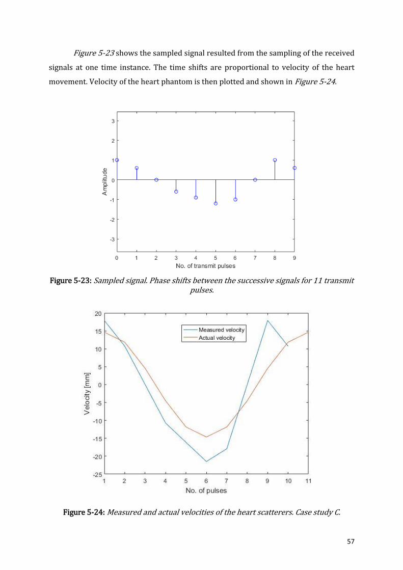
57

Figure 5-23 shows the sampled signal resulted from the sampling of the received

signals at one time instance. The time shifts are proportional to velocity of the heart

movement. Velocity of the heart phantom is then plotted and shown in Figure 5-24.

Figure 5-23: Sampled signal. Phase shifts between the successive signals for 11 transmit pulses.

Figure 5-24: Measured and actual velocities of the heart scatterers. Case study C.

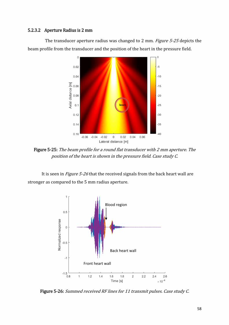
58

5.2.3.2 Aperture Radius is 2 mm

The transducer aperture radius was changed to 2 mm. Figure 5-25 depicts the

beam profile from the transducer and the position of the heart in the pressure field.

Figure 5-25: The beam profile for a round flat transducer with 2 mm aperture. The

position of the heart is shown in the pressure field. Case study C.

It is seen in Figure 5-26 that the received signals from the back heart wall are

stronger as compared to the 5 mm radius aperture.

Figure 5-26: Summed received RF lines for 11 transmit pulses. Case study C.

Blood region

Front heart wall

Back heart wall

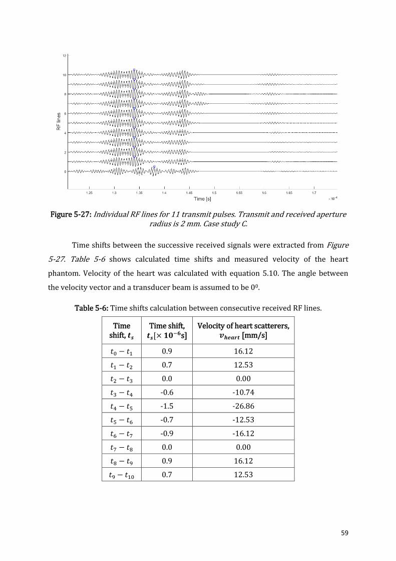
59

Figure 5-27: Individual RF lines for 11 transmit pulses. Transmit and received aperture radius is 2 mm. Case study C.

Time shifts between the successive received signals were extracted from Figure

5-27. Table 5-6 shows calculated time shifts and measured velocity of the heart

phantom. Velocity of the heart was calculated with equation 5.10. The angle between

the velocity vector and a transducer beam is assumed to be 00.

Table 5-6: Time shifts calculation between consecutive received RF lines.

Time shift, 𝒕𝒔

Time shift, 𝒕𝒔[× 𝟏𝟎−𝟔s]

Velocity of heart scatterers, 𝒗𝒉𝒆𝒂𝒓𝒕 [mm/s]

𝑡0 − 𝑡1 0.9 16.12

𝑡1 − 𝑡2 0.7 12.53

𝑡2 − 𝑡3 0.0 0.00

𝑡3 − 𝑡4 -0.6 -10.74

𝑡4 − 𝑡5 -1.5 -26.86

𝑡5 − 𝑡6 -0.7 -12.53

𝑡6 − 𝑡7 -0.9 -16.12

𝑡7 − 𝑡8 0.0 0.00

𝑡8 − 𝑡9 0.9 16.12

𝑡9 − 𝑡10 0.7 12.53

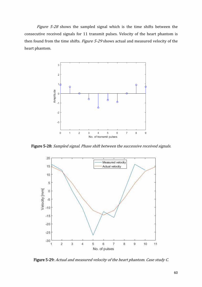
60

Figure 5-28 shows the sampled signal which is the time shifts between the

consecutive received signals for 11 transmit pulses. Velocity of the heart phantom is

then found from the time shifts. Figure 5-29 shows actual and measured velocity of the

heart phantom.

Figure 5-28: Sampled signal. Phase shift between the successive received signals.

Figure 5-29: Actual and measured velocity of the heart phantom. Case study C.

61

5.2.4 Case Study D

Heart phantom is placed further away from the transducer surface. Phantom is

moved to 2 cm away from the transducer surface. The distance between transducer and

the phantom is 10.7 cm. Figure 5-30 depicts B-mode image of the heart phantom

position. Figure 5-31 shows the beam profile of the transducer and the heart position in

the pressure field.

Figure 5-30: B-mode image of the phantom placed at 107 mm away from the transducer surface.

Figure 5-31: Beam profile for a transducer of 5 mm aperture. The heart is positioned in

the pressure field.

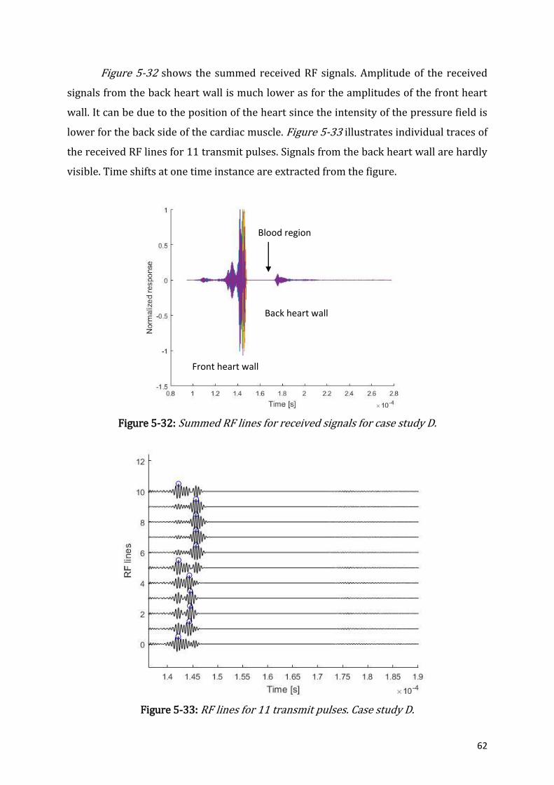
62

Figure 5-32 shows the summed received RF signals. Amplitude of the received

signals from the back heart wall is much lower as for the amplitudes of the front heart

wall. It can be due to the position of the heart since the intensity of the pressure field is

lower for the back side of the cardiac muscle. Figure 5-33 illustrates individual traces of

the received RF lines for 11 transmit pulses. Signals from the back heart wall are hardly

visible. Time shifts at one time instance are extracted from the figure.

Figure 5-32: Summed RF lines for received signals for case study D.

Figure 5-33: RF lines for 11 transmit pulses. Case study D.

Blood region

Front heart wall

Back heart wall

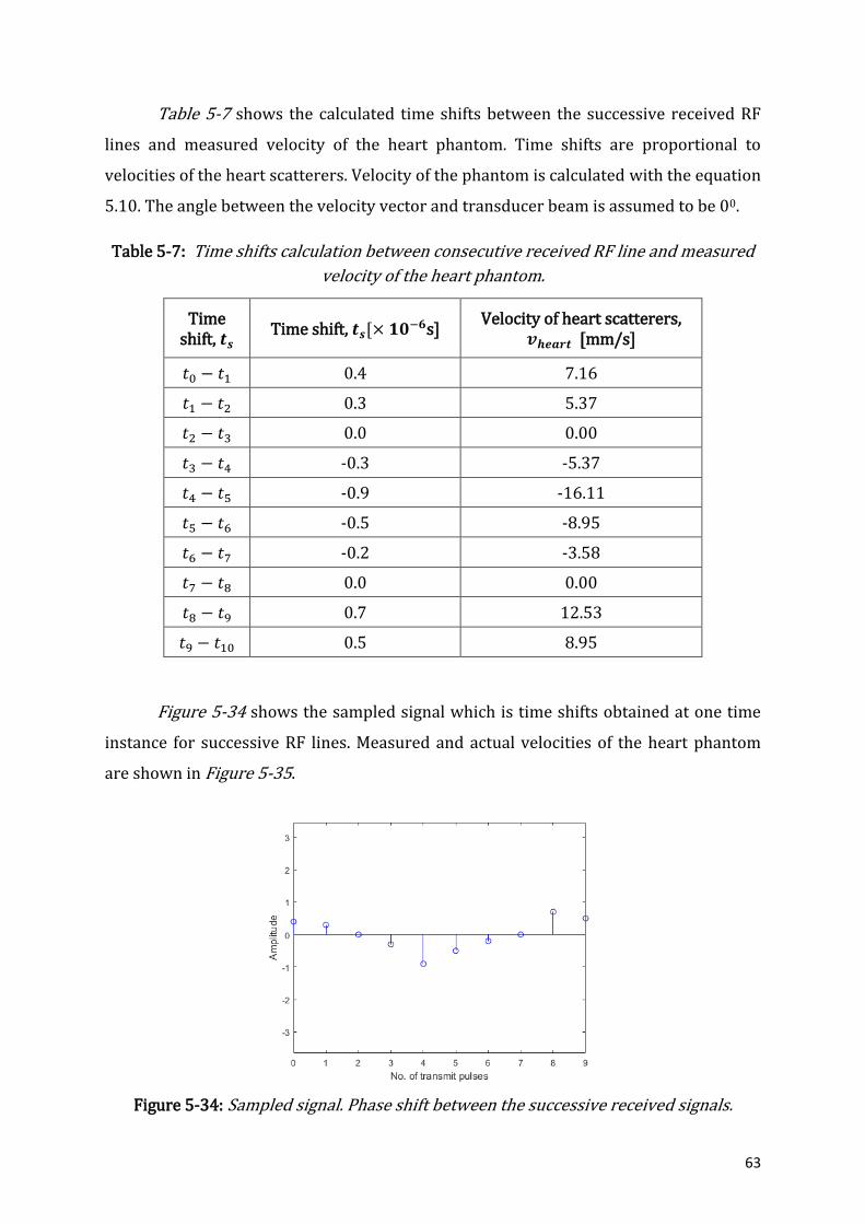
63

Table 5-7 shows the calculated time shifts between the successive received RF

lines and measured velocity of the heart phantom. Time shifts are proportional to

velocities of the heart scatterers. Velocity of the phantom is calculated with the equation

5.10. The angle between the velocity vector and transducer beam is assumed to be 00.

Table 5-7: Time shifts calculation between consecutive received RF line and measured

velocity of the heart phantom.

Time shift, 𝒕𝒔

Time shift, 𝒕𝒔[× 𝟏𝟎−𝟔s] Velocity of heart scatterers,

𝒗𝒉𝒆𝒂𝒓𝒕 [mm/s]

𝑡0 − 𝑡1 0.4 7.16

𝑡1 − 𝑡2 0.3 5.37

𝑡2 − 𝑡3 0.0 0.00

𝑡3 − 𝑡4 -0.3 -5.37

𝑡4 − 𝑡5 -0.9 -16.11

𝑡5 − 𝑡6 -0.5 -8.95

𝑡6 − 𝑡7 -0.2 -3.58

𝑡7 − 𝑡8 0.0 0.00

𝑡8 − 𝑡9 0.7 12.53

𝑡9 − 𝑡10 0.5 8.95

Figure 5-34 shows the sampled signal which is time shifts obtained at one time

instance for successive RF lines. Measured and actual velocities of the heart phantom

are shown in Figure 5-35.

Figure 5-34: Sampled signal. Phase shift between the successive received signals.

64

Figure 5-35: Measured and actual velocity of the heart phantom. Case study D.

5.3 Laboratory Work

Figure 5-36 shows the schematic representations of the transmit/receive

system. The hardware consists of pulse generator, receive/transmit, transducer input,

voltage gain amplifier, analog/digital converter and signal processing units. The set up

used to perform experiment is shown in Figure 5-37. The set up consists of the

transmit/receive hardware system, piezoelectric transducer and a computer. KB

Aerotech 2.25 MHz/13 mm non-focused transducer was used for measurements.

Resulting received digital signal is complex and can be written as[48]:

𝑟𝑠(𝑡) = 𝑥(𝑡) − 𝑗𝑦(𝑡). (5.13)

The phase is then found as [48]:

𝜑(𝑡) = 𝑎𝑟𝑐𝑡𝑎𝑛 (

𝑦(𝑡)

𝑥(𝑡)),

(5.14)

The phase difference between two consecutive signals is [48]:

∆𝜑(𝑖) = 𝜑(𝑖) − 𝜑(𝑖 − 1). (5.15)

There is another way to find a phase difference. The received signal can be multiplied

with a conjugate of the previous received signal [48]:

∆𝜑(𝑖) = 𝑎𝑟𝑐𝑡𝑎𝑛 (

𝑦(𝑖)

𝑥(𝑖)) ∙ 𝑎𝑟𝑐𝑡𝑎𝑛 (

𝑦(𝑖 − 1)

𝑥(𝑖 − 1)) .

(5.16)

65

This strategy was used to find the phase difference between the received signals.

Figure 5-36: Schematic representation of the transmit/receive system for ultrasound transducer.

Figure 5-37: Hardware set up for transmit and receive system for a transducer.

Round small and soft ball was taken for the experiment. The ball was placed into

the container with water. First, the transducer was moved up and down vertically and

phase shifts were displayed. Figure 5-38 shows two windows with resulted M-mode

image and phase shifts.

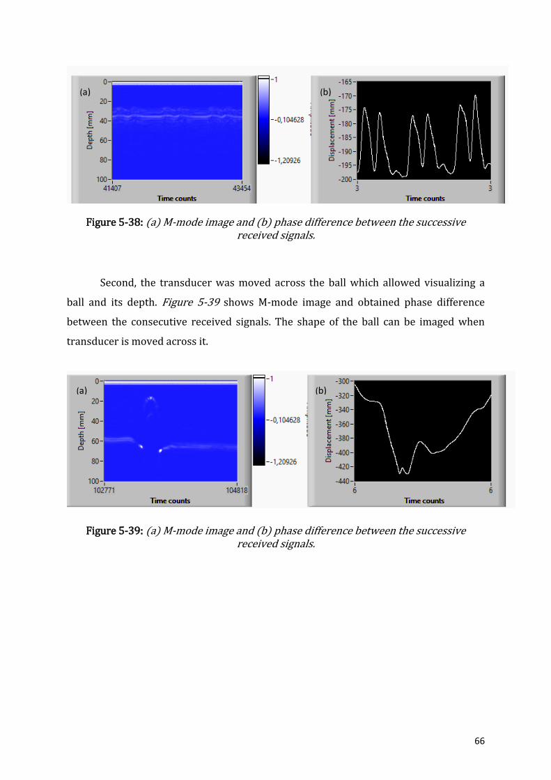
66

Figure 5-38: (a) M-mode image and (b) phase difference between the successive received signals.

Second, the transducer was moved across the ball which allowed visualizing a

ball and its depth. Figure 5-39 shows M-mode image and obtained phase difference

between the consecutive received signals. The shape of the ball can be imaged when

transducer is moved across it.

Figure 5-39: (a) M-mode image and (b) phase difference between the successive received signals.

(a) (b)

(a) (b)

67

6 DISCUSSION

Most of the stillbirths are preventable and depend on the access to a healthcare

and early detection. However, access to a healthcare is not always possible, especially in

low-income countries. Even in high-income countries, it is not always possible to

provide an immediate medical help to women who may complain about reduced fetal

movements [1], [80]. It is economically expensive to keep pregnant women in the

hospital if she feels worried about her baby. It is a common practice that pregnant

woman should return home if her worries were not justified. Therefore, it is important

to have a portable cheap device that can track fetal well-being independently of the

medical staff availability.

Fetus well-being can be evaluated by fetal movement observations and fetal

heart rate measurements. These are the first indicators of the fetus status that can be

used daily to judge fetus well-being. The counting of the fetal movements is a good

approach to observe the fetus. However, it is not a reliable technique. Fetal movement

assessment is affected by maternal perception of the fetus`s movements [23].

Continuous monitoring of the fetal heart rate is another way to monitor fetal health.

Fetal heart reactivity has a high association with fetal well-being and, therefore, fetal

heartbeat is a reliable way to judge fetus`s health status [17]. Doppler single-element

transducer can be implemented to track fetal heartbeat over time at home. They are

portable, easy in exploitation, reasonably cheap and accurate in heart rate

measurements. These transducers have good sensitivity and accuracy for heart rate

detection [81]. However, traditional Doppler transducers are only used by future

mothers or midwives to listen to a heartbeat for short period of time. In this thesis,

application of Doppler transducer was reconsidered. Traditional Doppler ultrasound

transducers due to their design are able to detect a heartbeat only if they are pointing

directly at the fetus heart. This research studied whether traditional Doppler transducer

will be able to track continuously a fetal heartbeat if it is attached to a woman`s

abdomen. Since the transducer will be attached for long time, the fetus may move and

the device itself may be displaced. Therefore, transducer should tolerate it and be able

to provide accurate results. Therefore, it was considered to design a transducer with a

smaller aperture in order to increase its robustness.

68

6.1 Simulations

This simulated Doppler ultrasound transducer operates by transmitting and

receiving acoustic echoes from the moving heart phantom. RF lines were recorded for

different positions of the scatterers over time instants. The scatterer motion was

tracked based on sampling over a defined time period. The background image was

static and the radii of the heart changed imitating a heartbeat. Received RF lines for

front heart wall have higher amplitudes as compared to the amplitudes of the received

signals from the back heart wall for all case studies. Since no attenuation was set in

Field II, the possible reason is that less energy propagates through the heart to the back

heart wall. The back heart wall is positioned in the pressure field with a lower intensity.

The time shifts between the successive RF line signals were used to analyse Doppler

shifts and to find velocity of the heart movement. The velocity of the heart phantom

movement was found from the sampled signal when one sample value is taken from

each RF line.

6.1.1 Case Study A and B

In case study A, heart is a highly scattered region and background is a weakly

scattered region. It was expected that simulated velocity of the heart phantom was close

to the theoretical values. However, the actual and measured velocities have slight

differences, especially for the measured velocity recorded with sixth transmitted pulse.

In case study B, background is now a highly scattered region and heart muscle is hardly

distinguishable in surrounding tissue. The measured and actual velocities have

differences. The possible reason is that the scattering may happen most likely from the

surrounding tissue rather than from the heart wall leading to non-accurate results for

received signals. Also, there are computational artifacts present during the simulations

that may lead to errors in calculating velocities. The simulation may not always give the

same results as theoretical calculations. The artifacts may come from the interaction of

the simulation tool with operational parameters and input data. Some of the

computational artifacts can be deduced from transmit and receive signals or spatial

impulse responses applied in Field II. The aperture of the transducer is divided into

mathematical elements and the responses from these elements are superimposed due

to linearity. The spatial impulse responses are calculated at the discrete points by taking

69

the difference from sample point to another sample point. The discrete time can be a

factor for the numerical artifacts. Quantitative analysis of the simulation errors was

performed by Jensen [82]. The accuracy of the pulse-echo response was found to be a

function of the sampling frequency.

Figure 6-1: The accuracy of the pulse-echo impulse response for rectangles and

bounding lines transducer elements as a function of the sampling frequency [82].

Rectangular transducer elements were used for the simulation and the sampling

frequency was set to 100 MHz. From the above Figure 6-1, it is seen that 100 MHz

sampling frequency will result in 20% relative error for accurate computations of the

received RF signals. Therefore, the accuracy of the simulation depends on the choice of

the sampling frequency. It is considered that increasing the sampling frequency

provides fine transmitted pulse which will results in accurate results for further

summations and convolutions operations. However, limitations should be applied for

the choice of the sampling frequency. First, high sampling frequency above 100 MHz

will result in increased number of samples to compute which may be a non-realistic

during the real-time performance. Second, Field II functions reliably with 100 MHz

sampling frequency and does better approximate calculations [62]. Third, the process of

finding sampling frequency arbitrary for each case can tedious and non-reliable.

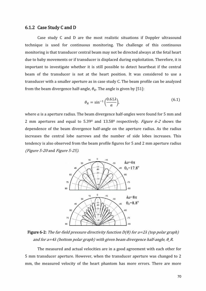
70

6.1.2 Case Study C and D

Case study C and D are the most realistic situations if Doppler ultrasound

technique is used for continuous monitoring. The challenge of this continuous

monitoring is that transducer central beam may not be directed always at the fetal heart

due to baby movements or if transducer is displaced during exploitation. Therefore, it is

important to investigate whether it is still possible to detect heartbeat if the central

beam of the transducer is not at the heart position. It was considered to use a

transducer with a smaller aperture as in case study C. The beam profile can be analyzed

from the beam divergence half-angle, 𝜃𝑅. The angle is given by [51]:

𝜃𝑅 = sin−1 (

0.61𝜆

𝑎),

(6.1)

where 𝑎 is a aperture radius. The beam divergence half-angles were found for 5 mm and

2 mm apertures and equal to 5.390 and 13.580 respectively. Figure 6-2 shows the

dependence of the beam divergence half-angle on the aperture radius. As the radius

increases the central lobe narrows and the number of side lobes increases. This

tendency is also observed from the beam profile figures for 5 and 2 mm aperture radius

(Figure 5-20 and Figure 5-25).

Figure 6-2: The far-field pressure directivity function D(θ) for a=2λ (top polar graph)

and for a=4λ (bottom polar graph) with given beam divergence half-angle, θ_R.

The measured and actual velocities are in a good agreement with each other for

5 mm transducer aperture. However, when the transducer aperture was changed to 2

mm, the measured velocity of the heart phantom has more errors. There are more

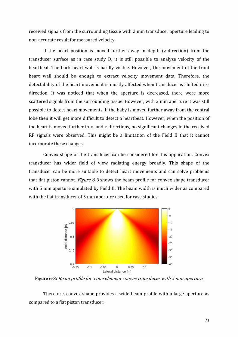
71

received signals from the surrounding tissue with 2 mm transducer aperture leading to

non-accurate result for measured velocity.

If the heart position is moved further away in depth (z-direction) from the

transducer surface as in case study D, it is still possible to analyze velocity of the

heartbeat. The back heart wall is hardly visible. However, the movement of the front

heart wall should be enough to extract velocity movement data. Therefore, the

detectability of the heart movement is mostly affected when transducer is shifted in x-

direction. It was noticed that when the aperture is decreased, there were more

scattered signals from the surrounding tissue. However, with 2 mm aperture it was still

possible to detect heart movements. If the baby is moved further away from the central

lobe then it will get more difficult to detect a heartbeat. However, when the position of

the heart is moved further in x- and z-directions, no significant changes in the received

RF signals were observed. This might be a limitation of the Field II that it cannot

incorporate these changes.

Convex shape of the transducer can be considered for this application. Convex

transducer has wider field of view radiating energy broadly. This shape of the

transducer can be more suitable to detect heart movements and can solve problems

that flat piston cannot. Figure 6-3 shows the beam profile for convex shape transducer

with 5 mm aperture simulated by Field II. The beam width is much wider as compared

with the flat transducer of 5 mm aperture used for case studies.

Figure 6-3: Beam profile for a one element convex transducer with 5 mm aperture.

Therefore, convex shape provides a wide beam profile with a large aperture as

compared to a flat piston transducer.

72

6.2 Laboratory work

Laboratory work was performed to analyse how single-element transducer

functions. Phase shifts between the received signals can be extracted from the moving

object. The test environment consists of the ball placed into container filled with water.

It was not possible to have any real-life environment as it would require a pregnant

woman to participate. Ultrasound is considered to be safe for a mother and a fetus.

However, at this stage of the research, it is not ethical to perform any real-life

experiments. This set up can be improved and used for further studies. Other types of

the transducers can be connected to a transmit/receive system. Based on the phase

shifts, this system is also able to produce M-mode image which also can be used to track

heart movements. M-mode imaging can be one of the options that can be included into

continuous monitoring system to track fetal well-being.

6.3 Ultrasound safety

Diagnostic ultrasound is considered to be a safe technique used in medicine.

Medical ultrasound offers many opportunities for diagnostics due to its impressive

safety [59]. The safety of ultrasound mainly depends on the magnitude of the

temperature elevation due to ultrasound exposure and the duration of the acoustic

exposure [83]. When it comes to the bio-effects induced by a transducer, 𝐼𝑆𝑃𝑇𝐴 is

introduced and stands for spatial peak temporal averaged intensity. 𝐼𝑆𝑃𝑇𝐴 is a power

divided by effective radiating area [59]. FDA approves 𝐼𝑆𝑃𝑇𝐴 to be 720 mW/cm2 [84].

Intensities less than 100 mW/cm2 do not generate heat regardless of the length of the

exposure [17]. Pulsed-wave Doppler transducer generate 1.5 to 5 mW/cm2 [17]. Also,

this Doppler ultrasound is a single-element unfocused piston-like transducer operating

at 2 MHz which is unlikely to excite any cavitation in fetal tissue [59]. However, more

research is required to study bio-effects for long term Doppler transducers monitoring.

73

7 CONCLUSION AND FUTURE WORK

The proposed idea to have a continuous fetal heartbeat monitoring is found to be

one of the solutions to reduce number of stillbirths. Discussions with midwives and

doctor from Horten Kommune Helsestasjon and also from literature [27], [5], [85], [86]

led to a conclusion that continuous monitoring can help to reduce pregnancy

complications and even stillbirth. Continuous monitoring will provide better tracking of

the fetus health and small changes of the fetus well-being will be recorded. Therefore,

pregnant women can get immediate help if it is required.

It is hard to adopt traditional Doppler ultrasound transducer for home use. The

robustness of the system can be improved if transducer aperture decreases. Wider

transducer beam will be able to catch the fetal heartbeat. However, transducer aperture

of 2 mm results only in 13.580 of beam divergence half-angle. Therefore, it may not be

always possible to detect fetal heartbeat due to the transducer displacement or fetus`s

movements. The system then becomes unreliable and problematic for long-term

monitoring.

Convex-shaped transducer is a promising device for a continuous fetal heartbeat

monitoring and also for future research topic. Both fetal heart rate and fetal movements

tracking can be a better solution to observe fetus well-being [87]. For example, fetal

movement assessment can be advanced by adopting an accelerometer. The system then

can be further advanced with the ability to analyse, record and transmit results for a

hospital review and evaluation. It also should be light and small and easy to be used for

a pregnant woman. Transmit/receive hardware system can then be used to perform

experimental work in a test environment and later in a real-life environment.

74

GLOSSARY

Amniotic fluid A fluid surrounding a fetus

Amniotic sac A fluid-filled sac that contains and protects a fetus in a womb

Diastole Part of the cardiac cycle when the heart refills with blood

Endocardium Inner layer of the heart wall that lines the chambers of the heart

Endometrium Inner membrane of the uterus

Epicardium Layer immediately outside of the myocardium heart muscle

Fundus Top portion of the uterus, located opposite to the cervix

Myocardium Middle layer of the heart wall

Pericardium Doubled-wall sac containing the heart and the roots of the great

vessels.

Perimetrium Outer layer of the uterus

Placenta Organ that connects the fetus to the uterine wall to allow

nutrient uptake

Pubic bone One of the bones that make up the pelvis

Systole Contraction phase of the cardiac cycle

Umbilical artery Paired artery that is found in the abdominal and pelvic regions.

It extends into the umbilical cord.

75

APPENDIX A: MATLAB CODE FOR A HEART PHANTOM IMAGE

% Calling: [positions, amp] = heart_phantom (N); % % Parameters: N - Number of scatterers in the phantom % % Output: positions - Positions of the scatterers. % amp - amplitude of the scatterers.

function [positions, amp] = heart_phantom (N)

x_size = 140/1000; % Width of phantom [mm] y_size = 30/1000; % Transverse width of phantom [mm] z_size = 160/1000; % Height of phantom [mm] z_start = 35/1000; % Start of phantom surface [mm];

% Create the general scatterers

x = (rand (N,1)-0.5)*x_size; y = (rand (N,1)-0.5)*y_size; z = rand (N,1)*z_size + z_start;

% Generate the amplitudes with a Gaussian distribution

amp=10*randn(N,1);

% Make the heart and set the amplitudes to zero inside

% heart radii r1=18/1000; % Radii [mm] r2=16/1000; xc=0/1000; % Place of heart [mm] zc=90/1000+z_start;

inside=((x-xc).^2+(z-zc).^2)<r1^2; inside=inside.*((x-xc).^2+(z-zc).^2)>r2^2;

A_heart=1;

ampHEART=amp.*inside*A_heart;

ampMEDIUM=amp.*(inside-1);

amp=ampHEART+ampMEDIUM;

inside = ( ((x-xc).^2 + (z-zc).^2) < r2^2); amp = amp .* (1-inside);

positions=[x y z];

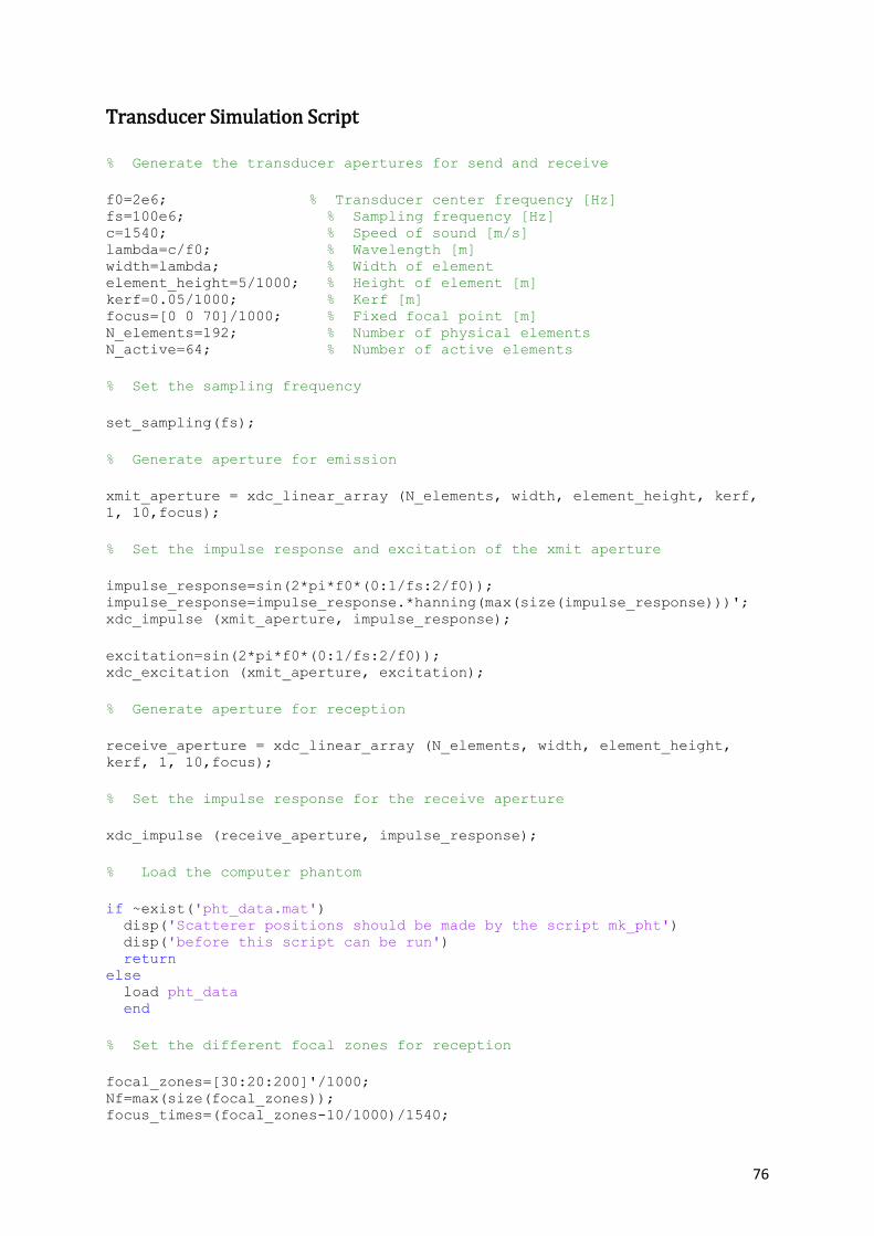
76

Transducer Simulation Script

% Generate the transducer apertures for send and receive

f0=2e6; % Transducer center frequency [Hz] fs=100e6; % Sampling frequency [Hz] c=1540; % Speed of sound [m/s] lambda=c/f0; % Wavelength [m] width=lambda; % Width of element element_height=5/1000; % Height of element [m] kerf=0.05/1000; % Kerf [m] focus=[0 0 70]/1000; % Fixed focal point [m] N_elements=192; % Number of physical elements N_active=64; % Number of active elements

% Set the sampling frequency

set_sampling(fs);

% Generate aperture for emission

xmit_aperture = xdc_linear_array (N_elements, width, element_height, kerf,

1, 10,focus);

% Set the impulse response and excitation of the xmit aperture

impulse_response=sin(2*pi*f0*(0:1/fs:2/f0)); impulse_response=impulse_response.*hanning(max(size(impulse_response)))'; xdc_impulse (xmit_aperture, impulse_response);

excitation=sin(2*pi*f0*(0:1/fs:2/f0)); xdc_excitation (xmit_aperture, excitation);

% Generate aperture for reception

receive_aperture = xdc_linear_array (N_elements, width, element_height,

kerf, 1, 10,focus);

% Set the impulse response for the receive aperture

xdc_impulse (receive_aperture, impulse_response);

% Load the computer phantom

if ~exist('pht_data.mat') disp('Scatterer positions should be made by the script mk_pht') disp('before this script can be run') return else load pht_data end

% Set the different focal zones for reception

focal_zones=[30:20:200]'/1000; Nf=max(size(focal_zones)); focus_times=(focal_zones-10/1000)/1540;

77

z_focus=60/1000; % Transmit focus

% Set the apodization

apo=hanning(N_active)';

% Do linear array imaging

no_lines=120; % Number of lines in image image_width=80/1000; % Size of image sector d_x=image_width/no_lines; % Increment for image

% Do imaging line by line

for i=[1:no_lines]

% Test if the file for the line exist. % Skip the simulation, if the line exits and % go the next line. Else make the simulation

file_name=['rf_data/rf_ln',num2str(i),'.mat'];

if ~exist(file_name)

% Save a file to reserve the calculation

cmd=['save rf_data/rf_ln',num2str(i),'.mat i']; eval(cmd);

disp(['Now making line ',num2str(i)])

% The the imaging direction

x= -image_width/2 +(i-1)*d_x;

% Set the focus for this direction with the proper reference point

xdc_center_focus (xmit_aperture, [x 0 0]); xdc_focus (xmit_aperture, 0, [x 0 z_focus]); xdc_center_focus (receive_aperture, [x 0 0]); xdc_focus (receive_aperture, focus_times, [x*ones(Nf,1), zeros(Nf,1),

focal_zones]);

% Calculate the apodization

N_pre = round(x/(width+kerf) + N_elements/2 - N_active/2); N_post = N_elements - N_pre - N_active; apo_vector=[zeros(1,N_pre) apo zeros(1,N_post)]; xdc_apodization (xmit_aperture, 0, apo_vector); xdc_apodization (receive_aperture, 0, apo_vector);

% Calculate the received response

[rf_data, tstart]=calc_scat(xmit_aperture, receive_aperture,

phantom_positions, phantom_amplitudes);

% Store the result

78

cmd=['save rf_data/rf_ln',num2str(i),'.mat rf_data tstart']; disp(cmd) eval(cmd); else disp(['Line ',num2str(i),' is being made by another machine.']) end end

% Free space for apertures

xdc_free (xmit_aperture) xdc_free (receive_aperture)

disp('You should now run make_image to display the image')

Make Image Script

f0=2e6; % Transducer center frequency [Hz] fs=100e6; % Sampling frequency [Hz] c=1540; % Speed of sound [m/s] no_lines=120; % Number of lines in image image_width=140/1000; % Size of image sector d_x=image_width/no_lines; % Increment for image

% Read the data and adjust it in time

min_sample=0; for i=1:no_lines

% Load the result

cmd=['load rf_data/rf_ln',num2str(i),'.mat']; disp(cmd) eval(cmd)

% Find the envelope

rf_env=abs(hilbert([zeros(round(tstart*fs-min_sample),1); rf_data])); env(1:max(size(rf_env)),i)=rf_env; end

% Do logarithmic compression

D=10; % Sampling frequency decimation factor dB_range=50; % Dynamic range for display in dB

disp('Finding the envelope') log_env=env(1:D:max(size(env)),:)/max(max(env)); log_env=20*log10(log_env); log_env=127/dB_range*(log_env+dB_range);

% Make an interpolated image

79

disp('Doing interpolation') ID=20; [n,m]=size(log_env); new_env=zeros(n,m*ID); for i=1:n new_env(i,:)=interp(log_env(i,:),ID); end [n,m]=size(new_env);

fn=fs/D; clf image(((1:(ID*no_lines-1))*d_x/ID-

no_lines*d_x/2)*1000,((1:n)/fn+min_sample/fs)*1540/2*1000,new_env) xlabel('Lateral distance [mm]') ylabel('Axial distance [mm]') colormap(gray(128)) axis('image') axis([-70 70 35 160])

80

APPENDIX B: MATLAB CODES USED FOR CASE STUDY A, B, C & D

%% Main script to simulate heart wall movements and to receive RF lines clc; clear; close all;

%% variables N = 200000; f_heart = 2.33; Thm = 1/f_heart; Nhm = 10; %Number of transmit pulses=Nhm+1 t_2bps=[0:Thm/Nhm:Thm]; %t_2bps=[0 0 0 0 0 0 0 0 0 0 0];

r1=(18 + 1*sin(2*pi*f_heart*(t_2bps)))./1000; r2=(16 + 1*sin(2*pi*f_heart*(t_2bps)))./1000;

% create struct results = struct(); % empty struct %%

for ii = 1:length(r1) % call function heart_pht [phantom_positions, phantom_amplitudes] = heart_pht(N, r1(ii), r2(ii)); save pht_data.mat phantom_positions phantom_amplitudes

% call script sim_img %sim_img;

% call script make_image %make_image;

% call script single_el_tr_pulse signle_el_tr_pulse;

% allocate data to struct results(ii).v = v; results(ii).t = t; results(ii).t2 = t2;

end %% figure(91); hold on for ii =0:size(results,2)-1 %plot(results(ii+1).t2, ii+abs(hilbert(results(ii+1).v./2)), 'k') plot(results(ii+1).t2, ii+((results(ii+1).v./2)), 'k') [tmax, indtmax] = max(results(ii+1).v); plot(results(ii+1).t2(indtmax), ii+results(ii+1).v(indtmax)./2, 'ob') xlabel('Time [s]', 'FontSize', 12) ylabel('RF lines', 'Fontsize', 12) end [tmax, indtmax] = max(results(1).v); plot([results(1).t2(indtmax), results(1).t2(indtmax)], [0, ii+1], 'r')

xlim([1.1e-4, 1.8e-4])

save('results', 'results')

81

Script for Transducer Simulation

% Set initial parameters f0=2e6; % Transducer center frequency [Hz] fs=100e6; % Sampling frequency [Hz] % c=1540; % Speed of sound [m/s] % lambda=c/f0; % Wavelength [m] R=5/1000; element_size=1/1000; M=5;

% Define the transducer Th=xdc_piston(R, element_size);

% Set the impulse response and excitation of the emit aperture impulse_response=sin(2*pi*f0*(0:1/fs:3/f0)); impulse_response=impulse_response.*hanning(max(size(impulse_response)))';

xdc_impulse (Th, impulse_response);

excitation=sin(2*pi*f0*(0:1/fs:M/f0)); xdc_excitation (Th, excitation); % Do the calculation [v,t]=calc_scat_multi(Th, Th, phantom_positions, phantom_amplitudes);

%calculate the received signals from the collections of scatterers for all

the elements in the aperture

% Plot the individual responses [N,M]=size(v) v=v/max(max(v)); figure(1); hold on plot((0:N-1)/fs+t,v)

% hold off %title('Individual traces') xlabel('Time [s]') ylabel('Normalized response')

%% update t t2 = (0:N-1)/fs+t;

%%

L=length(v); nfft = 2^nextpow2(10*L); f=fs.*[-nfft/2:1:nfft/2-1]/nfft; V=2*fft(v,nfft)/L; % V = V(nfft/2:end); figure(2); hold on plot(f/1e6, fftshift(abs(V))); xlim([0,5]); xlabel('f [MHz]') ylabel('Amplitude')

82

APPENDIX C: MATLAB CODE FOR M-MODE IMAGE

f0=2e6; % Transducer center frequency [Hz] fs=100e6; % Sampling frequency [Hz] c=1540; % Speed of sound [m/s] no_lines=1; % Number of lines in image image_width=60/1000; % Size of image sector d_x=image_width/no_lines; % Increment for image

% Load the result

min_sample=0; dynamicRange=17; %load('Result\Info.mat'); i=1; for time=0:1:length(t_2bps)-1 fileName=sprintf('rf_data\\rf_ln%i.mat',i); load(fileName,'rf_data'); echo=rf_data; %echo=-echo(1:1:ti*fs); %rf_env=abs(hilbert([zeros(round(time*fs-

min_sample),1);echo])); echo=echo(1:1:length(echo)); rf_env=abs(hilbert(echo)); env(1:size(rf_env,1),i+1)=rf_env; i=i+1; end

numberOfLines=i; c=1540; env_dB=20*log10(env); env_dB=env_dB-max(max(env_dB)); env_gray=127*(env_dB+dynamicRange)./dynamicRange; %env_gray = env; depth=((0:size(env,1)-1)+min_sample)/fs*c/2;

x=t_2bps; figure imagesc(x,(depth*1000),env_gray,[0 dynamicRange]); xlabel('No. of transmit pulses'); ylabel('Depth [mm]'); colormap(gray(128)); colorbar('XTick',0,'XTickLabel','Power(dB)'); hold off

83

APPENDIX D: FLAT PISTON TRANSDUCER BEAM PROFILE

function Th=define_transducer(TR) % function Th=define_transducer(TR) % % Define transducer for use in Field II % % TR Struct containing transducer specification % Th Pointer to transducer aperture, from Field II

%--- Geometry --- % Round flat aperture following Field II specification ele_size=0.2/1000; radius=5/1000; Th=xdc_piston(radius, ele_size);

%--- Pulse --- excitation=sin(2*pi*TR.f0*(0:1/TR.fs:5/TR.f0)); xdc_excitation (Th, excitation);

%--- Transmit aperture --- % Impulse response approximated as Hanning-windowed sine-pulse

impulse_response=sin(2*pi*TR.f0*(0:1/TR.fs:3/TR.f0)); impulse_response=impulse_response.*hanning(max(size(impulse_response)))'; xdc_impulse(Th, impulse_response);

%--- Receive aperture --- xdc_impulse(Th, impulse_response);

return

%=== Constants ========================================================== c = 1540; % m/s Speed of sound in fluid

%=== Transducer Definition ============================================== % 'TR' is a struct containing transducer specification TR.fs = 100e6; % Hz Sample rate TR.f0 = 2e6; % Hz Transducer center frequency

Th = define_transducer(TR); set_sampling(TR.fs);

%=== Calculate and plot tranducer field ================================== TR= calculate_and_plot(TR, Th, [70 160]*1e-3); %title( sprintf('Frequency %.1f MHz. Width %.0f mm', TR.f0/1e6, TR.W*1e3) )

%=== Clean up and quit =================================================== xdc_free(Th)

return

84

Appendix E: LABVIEW ‘Process’ state

85

REFERENCES

[1] L. De Bernis, M. V Kinney, W. Stones, P. Ten Hoope-Bender, D. Vivio, S. H. Leisher, Z. Qar,

A. Bhutta, M. Gülmezoglu, M. Mathai, J. M. Belizán, L. Franco, L. Mcdougall, J. Zeitlin, A.

Malata, K. E. Dickson, and J. E. Lawn, “Stillbirths: ending preventable deaths by 2030,”

Lancet, vol. 387, pp. 703–716, 2016.

[2] “WHO | Stillbirths,” 2015. [Online]. Available:

http://www.who.int/maternal_child_adolescent/epidemiology/stillbirth/en/. [Accessed:

06-Sep-2015].

[3] “Stillbirth - Introduction - NHS Choices.” [Online]. Available:

http://www.nhs.uk/conditions/Stillbirth/Pages/Definition.aspx. [Accessed: 06-Sep-

2015].

[4] E. O’Neill and J. Thorp, “Antepartum evaluation of the fetus and fetal well being.,” Clin.

Obstet. Gynecol., vol. 55, no. 3, pp. 722–30, Sep. 2012.

[5] A. Vais and L. Kean, “Stillbirth in the UK: current trends, investigation and opportunities

for prevention,” Obstet. Gynaecol. Reprod. Med., vol. 25, no. 6, pp. 160–166, 2015.

[6] R. A. Haws, M. Y. Yakoob, T. Soomro, E. V Menezes, G. L. Darmstadt, and Z. A. Bhutta,

“Reducing stillbirths: screening and monitoring during pregnancy and labour.”

[7] “The American College of Obstetricians and Gynecologists,” 2016. [Online]. Available:

http://www.acog.org/Patients/FAQs/Special-Tests-for-Monitoring-Fetal-Health.

[8] “Home foetal heart monitors ‘risky,’” NHS Choices, 2009. [Online]. Available:

http://www.nhs.uk/news/2009/11November/Pages/Home-foetal-heart-monitors-

risky.aspx. [Accessed: 09-Sep-2015].

[9] K. J. Gibbins, R. M. Silver, H. Pinar, U. M. Reddy, C. B. Parker, V. Thorsten, M. Willinger, D. J.

Dudley, R. Bukowski, G. R. Saade, M. A. Koch, D. Conway, C. J. Hogue, B. J. Stoll, and R. L.

Goldenberg, “Stillbirth, hypertensive disorders of pregnancy, and placental pathology,”

Placenta, vol. 43, pp. 61–68, 2016.

[10] “Special Tests for Monitoring Fetal Health - ACOG.” [Online]. Available:

http://www.acog.org/Patients/FAQs/Special-Tests-for-Monitoring-Fetal-Health.

[Accessed: 05-Sep-2015].

[11] R. A. Haws, M. Y. Yakoob, T. Soomro, E. V Menezes, G. L. Darmstadt, and Z. A. Bhutta,

“Reducing stillbirths: screening and monitoring during pregnancy and labour.,” BMC

86

Pregnancy Childbirth, vol. 9 Suppl 1, no. Suppl 1, p. S5, Jan. 2009.

[12] A. Y. Elzouki, H. A. Harfi, F. B. Stapleton, H. Nazer, W. Oh, and R. J. Whitley, Textbook of

Clinical Pediatrics. Springer Science & Business Media, 2012.

[13] B. Winje, E. Saastad, N. Gunnes, J. Tveit, B. Stray-Pedersen, V. Flenady, and J. Frøen,

“Analysis of ‘count-to-ten’ fetal movement charts: a prospective cohort study,” BJOG An

Int. J. Obstet. Gynaecol., vol. 118, no. 10, pp. 1229–1238, 2011.

[14] L. Mangesi and G. J. Hofmeyr, “Fetal movement counting for assessment of fetal

wellbeing.,” Cochrane database Syst. Rev., no. 1, p. CD004909, Jan. 2007.

[15] “Non-Stress Test (NST).” [Online]. Available:

http://www.hopkinsmedicine.org/gynecology_obstetrics/specialty_areas/maternal_fetal

_medicine/services/antepartum_testing_prenatal_diagnosis_treatment_center/non_stres

s_test.html. [Accessed: 06-Sep-2015].

[16] Fetal Heart Monitoring: Principles and Practices. Kendall Hunt, 1993.

[17] R. K. Freeman, T. J. Garite, M. P. Nageotte, and L. A. Miller, Fetal Heart Rate Monitoring.

Lippincott Williams & Wilkins, 2012.

[18] J. P. Phelan, M. O. Ahn, C. V Smith, S. E. Rutherford, and E. Anderson, “Amniotic fluid index

measurements during pregnancy.,” J. Reprod. Med., vol. 32, no. 8, pp. 601–4, Aug. 1987.

[19] L. Littleton-Gibbs and J. Engebretson, Maternity Nursing Care. Cengage Learning, 2012.

[20] K. Whitaker, P. Eberle, and L. Trujillo, Comprehensive Perinatal & Pediatric Respiratory

Care. Cengage Learning, 2014.

[21] M. I. Levene and F. A. Chervenak, Fetal and Neonatal Neurology and Neurosurgery.

Elsevier Health Sciences, 2009.

[22] Doppler Ultrasound in Obstetrics and Gynecology. Springer Science & Business Media,

2006.

[23] J. F. Frøen, A. E. P. Heazell, J. V. H. Tveit, E. Saastad, R. C. Fretts, and V. Flenady, “Fetal

Movement Assessment,” Semin. Perinatol., vol. 32, no. 4, pp. 243–246, 2008.

[24] E. K. Cydney Afriat Menihan, Electronic Fetal Monitoring: Concepts and Applications.

Lippincott Williams & Wilkins, 2007.

[25] WebMD, “High-risk pregnancy,” 2016. [Online]. Available:

http://www.webmd.com/baby/checking-fetus-in-high-risk-pregnancy. [Accessed: 03-

Mar-2016].

87

[26] A. Biswas, S. Biswas, A. Cum Mo, M. Walliullah, and A. K. Mukhopadhyay, “Indian Medical

Gazette Role of Non Stress Test in Monitoring High Risk Pregnancy,” 2013.

[27] R. Brown, J. H. B. Wijekoon, A. Fernando, E. D. Johnstone, and A. E. P. Heazell, “Continuous

objective recording of fetal heart rate and fetal movements could reliably identify fetal

compromise, which could reduce stillbirth rates by facilitating timely management,” Med.

Hypotheses, vol. 83, no. 3, pp. 410–417, 2014.

[28] T. R. Moore, “The Role of Amniotic Fluid Assessment in Evaluating Fetal Well-Being.”

[29] Ronald S. Gibbs, Danforth’s Obstetrics and Gynecology. Lippincott Williams & Wilkins,

2008.

[30] R. Gagnon, M. Van den Hof, H. N. Stephen Bly, O. O. Duncan Farquharson, V. B. Robert

Gagnon, L. O. Barbara Lewthwaite, W. M. Lucie Morin, M. Q. Shia Salem, and A. Skoll, “THE

USE OF FETAL DOPPLER IN OBSTETRICS,” J Obs. Gynaecol Can, vol. 25(7), 2003.

[31] R. L. Goldenberg, E. M. McClure, A. H. Jobe, B. D. Kamath-Rayne, M. G. Gravette, and C. E.

Rubens, “Stillbirths and neonatal mortality as outcomes,” Int. J. Gynecol. Obstet., vol. 123,

no. 3, pp. 252–253, 2013.

[32] G. Pagani, F. D’Antonio, A. Khalil, A. Papageorghiou, A. Bhide, and B. Thilaganathan,

“Association between reduced fetal movements at term and first trimester markers of

impaired placental development,” Placenta, vol. 35, no. 8, pp. 606–610, 2014.

[33] c and Ernst Beinder, MD,a Tomas Grancay,a Theresa Menéndez, MD,b Helmut Singer, MD

and Md. Michael Hofbeck, “Fetal sinus bradycardia and the long QT syndrome,” Am J Obs.

Gynecol, vol. 185, no. 3.

[34] P. G. Pézard, F. Boussion, L. Sentilhes, C. Lépinard, M.-H. Couvreur, J. Victor, P. Geslin, and

P. Descamps, “Fetal tachycardia: A role for amiodarone as first- or second-line therapy?,”

Arch. Cardiovasc. Dis., vol. 101, no. 10, pp. 619–627, 2008.

[35] “How can I monitor my baby’s movements? | Count the Kicks.” [Online]. Available:

http://www.countthekicks.org.uk/mums/your-babys-movements/how-to-monitor-

babys-movements/. [Accessed: 09-Sep-2015].

[36] “Products | Count the Kicks.” [Online]. Available:

http://www.countthekicks.org.uk/shop/. [Accessed: 09-Sep-2015].

[37] “Kick Counter Wristband | Count the Kicks.” [Online]. Available:

http://www.countthekicks.org.uk/shop/kick-counter-wristband/. [Accessed: 09-Sep-

2015].

88

[38] “Kickme - Baby Kicks Counter – Android Apps on Google Play.” [Online]. Available:

https://play.google.com/store/apps/details?id=com.dilmeapps.kickme&hl=en_GB.

[Accessed: 09-Sep-2015].

[39] “Popamazing LCD Prenatal Fetal Doppler Angel Heart Sound Monitor Backlight Screen

Display CE & EC Medical Directive: Amazon.co.uk: Baby.” [Online]. Available:

http://www.amazon.co.uk/dp/B00SM7LWFK?psc=1. [Accessed: 09-Sep-2015].

[40] “Baby Heartbeat Listener – Android Apps on Google Play.” [Online]. Available:

https://play.google.com/store/apps/details?id=com.lema.android.babyheartbeatlistene

r&hl=en_GB. [Accessed: 09-Sep-2015].

[41] “BBC NEWS | Health | Foetal heart rate monitor warning.” [Online]. Available:

http://news.bbc.co.uk/2/hi/health/8343317.stm. [Accessed: 09-Sep-2015].

[42] S. Bhong and S. D. Lokhande, “Wireless Fetal Monitoring,” Int. J. Sci. Res., vol. 2, no. 3, pp.

2319–7064, 2013.

[43] I. Clausen and T. Glott, “Development of Clinically Relevant Implantable Pressure

Sensors: Perspectives and Challenges.,” Sensors (Basel)., vol. 14, no. 9, pp. 17686–17702,

Jan. 2014.

[44] A. J. Wolfberg, “The future of fetal monitoring.,” Rev. Obstet. Gynecol., vol. 5, no. 3–4, pp.

e132–6, 2012.

[45] Q. Plummer, “Wireless Fetal Monitoring System Gets Feds Blessings, Boasts Advanced

Features,” Tech Times, 2015. [Online]. Available:

http://www.techtimes.com/articles/25689/20150113/fda-clears-marketing-of-

wireless-system-for-fetal-monitoring.htm. [Accessed: 11-Sep-2015].

[46] A. A. Boatin, B. Wylie, I. Goldfarb, R. Azevedo, E. Pittel, C. Ng, and J. Haberer, “Wireless

fetal heart rate monitoring in inpatient full-term pregnant women: testing functionality

and acceptability.,” PLoS One, vol. 10, no. 1, p. e0117043, Jan. 2015.

[47] T. L. Szabo and T. L. Szabo, “3 – ACOUSTIC WAVE PROPAGATION,” in Diagnostic

Ultrasound Imaging, 2004, pp. 47–70.

[48] Jørgen Arendt Jensen, Estimation of Blood Velocities Using Ultrasound A Signal

Processing Approach. Technical University of Denmark: Cambridge University Press,

1996.

[49] Jørgen Arendt Jensen, Estimation of Blood Velocities Using Ultrasound A Signal

Processing Approach. Technical University of Denmark, Lyngby: Cambridge University

Press, 1996.

89

[50] T. L. Szabo and T. L. Szabo, “1 – INTRODUCTION,” in Diagnostic Ultrasound Imaging,

2004, pp. 1–28.

[51] R. S. C. Cobbold, Foundations of biomedical ultrasound. Oxford University Press, 2007.

[52] B. Fay, “Ultrasonic Backscattering: Fundamentals and Applications,” Phys. Acoust., pp.

41–53, 1991.

[53] T. L. Szabo and T. L. Szabo, “4 – ATTENUATION,” in Diagnostic Ultrasound Imaging, 2004,

pp. 71–95.

[54] S. Cochran, “Piezoelectricity and basic configurations for piezoelectric ultrasonic

transducers,” in Ultrasonic Transducers, 2012, pp. 3–35.

[55] FERROPERM, “Pz27 (Navy II) A soft PZT with low ageing rates and high sensitivity.” .

[56] J. E. Wilhjelm, M. Kristensson, and O. T. Andersen, “Medical diagnostic ultrasound

physical principles and imaging,” 2010.

[57] T. L. Szabo and T. L. Szabo, “11 – DOPPLER MODES,” in Diagnostic Ultrasound Imaging,

2004, pp. 337–380.

[58] G. S. Reeder, P. J. Currie, D. J. Hagler, A. J. Tajik, and J. B. Seward, “Use of Doppler

techniques (continuous-wave, pulsed-wave, and color flow imaging) in the noninvasive

hemodynamic assessment of congenital heart disease,” Mayo Clin Proc, vol. 61, no. 9, pp.

725–744, Sep. 1986.

[59] T. L. Szabo and T. L. Szabo, “15 – ULTRASOUND-INDUCED BIOEFFECTS,” in Diagnostic

Ultrasound Imaging, 2004, pp. 489–516.

[60] T. R. Nelson, J. B. Fowlkes, J. S. Abramowicz, and C. C. Church, “Ultrasound biosafety

considerations for the practicing sonographer and sonologist.,” J. Ultrasound Med., vol.

28, no. 2, pp. 139–50, Feb. 2009.

[61] “510(k) Summary of Safety and Effectiveness I90-IYO,” 2009.

[62] J. A. Jensen, “Users’ guide for the Field II program.”

[63] J. A. Jensen, “Field: A Program for Simulating Ultrasound Systems,” Publ. Med. Biol. Eng.

Comput., vol. 34, no. 1, pp. 351–353, 1996.

[64] M. Schlaikjer, S. Torp-Pedersen, and J. A. Jensen, “Simulation of RF data with tissue

motion for optimizing stationary echo canceling filters.”

[65] M. A. Lediju, M. J. Pihl, J. J. Dahl, and G. E. Trahey, “Quantitative assessment of the

magnitude, impact and spatial extent of ultrasonic clutter.,” Ultrason. Imaging, vol. 30, no.

3, pp. 151–68, Jul. 2008.

90

[66] J. A. Jensen and S. I. Nikolov, “Fast Simulation of Ultrasound Images.”

[67] Johan Kirkhorn, “Introduction to IQ-demodulation of RF-data.”

[68] J. N. The Boston Women’s Health Book Collective, Our Bodies, Ourselves: Pregnancy and

Birth. Simon and Schuster, 2008.

[69] D. Shimon, “Myometrial Thickness in Pregnancy :,” J. Ultrasound Med., pp. 661–665, 1998.

[70] N. B. Hershfield, “The Abdominal Wall,” J. Clin. Gastroenterol., vol. 14, no. 3, pp. 199–202,

1992.

[71] L. Lancerotto, C. Stecco, V. MacChi, A. Porzionato, A. Stecco, and R. De Caro, “Layers of the

abdominal wall: Anatomical investigation of subcutaneous tissue and superficial fascia,”

Surg. Radiol. Anat., vol. 33, no. 10, pp. 835–842, 2011.

[72] E. Zohav, A. Dunsky, O. Segal, R. Peled, A. Herman, and S. Segal, “The effects of maternal

and fetal parameters on the quality of nuchal translucency measurement,” pp. 638–640,

2001.

[73] “WOMEN AND NEWBORN HEALTH SERVICE MEASURING FUNDAL HEIGHT WITH A

TAPE MEASURE,” King Edward Memorial Hospital. [Online]. Available:

http://www.kemh.health.wa.gov.au/development/manuals/O&G_guidelines/sectionb/1

/b1.6.3.pdf. [Accessed: 10-Mar-2016].

[74] S. Kunii, J. Sugawara, Y. Kimura, N. Imai, H. Chisaka, H. Hasegawa, Y. Koiwa, H. Kanai, and

K. Okamura, “Fetal Myocardial Thickening Measured by Ultrasonic-Based Technique

Called ‘Phased-Tracking Method,’” Fetal Diagn Ther, vol. 21, pp. 458–465, 2006.

[75] C. Firpo, J. I. E. Hoffman, and N. H. Silverman, “Evaluation of Fetal Heart Dimensions from

12 Weeks to Term,” Am J Cardiol, vol. 87, pp. 594–600, 2001.

[76] S. L. Kuntharee Traisrisilp, Fuanglada Tongprasert, Kasemsri Srisupundit and M. Theera

Tongsong, “Reference Ranges for the Fetal Cardiac Circumference Derived by Cardio–

Spatiotemporal Image Correlation From 14 to 40 Weeks’ Gestation,” J Ultrasound Med,

vol. 30, pp. 1191–1196, 2011.

[77] S. Luewan, Y. Yanase, F. Tongprasert, K. Srisupundit, and T. Tongsong, “Fetal cardiac

dimensions at 14-40 weeks’ gestation obtained using cardio-STIC-M,” Ultrasound Obstet.

Gynecol., vol. 37, no. 4, pp. 416–422, 2011.

[78] “Cardiac screening examination of the fetus: guidelines for performing the ‘basic’ and

‘extended basic’ cardiac scan,” Ultrasound Obs. Gynecol, vol. 27, pp. 107–113, 2006.

[79] T. L. Szabo and T. L. Szabo, “8 – WAVE SCATTERING AND IMAGING,” in Diagnostic

Ultrasound Imaging, 2004, pp. 213–242.

91

[80] P. Vergani, S. Cozzolino, E. Pozzi, M. S. Cuttin, M. Greco, S. Ornaghi, and V. Lucchini,

“Identifying the causes of stillbirth: a comparison of four classification systems,” Am. J.

Obstet. Gynecol., vol. 199, no. 3, pp. 319.e1–319.e4, 2008.

[81] A. Mert, M. Sezd ˙ I, and A. Akan, “A test and simulation device for Doppler-based fetal

heart rate monitoring,” vol. 23, pp. 1187–1194, 2015.

[82] J. A. Jensen, “Speed-accuracy trade-offs in computing spatial impulse responses for

simulating medical ultrasound imaging,” Publ. J. Comput. Acoust., vol. 9, no. 3, pp. 731–

744, 2001.

[83] H. Azhari, “CH12: Safety and therapeutic applications,” pp. 287–312.

[84] D. L. Miller, “Safety Assurance in Obstetrical Ultrasound,” Semin. Ultrasound, CT MRI, vol.

29, no. 2, pp. 156–164, 2008.

[85] P. ten Hoope-Bender, K. Stenberg, and K. Sweeny, “Reductions in stillbirths a more than a

triple return on investment,” Lancet, vol. 387, pp. e14–e16, 2016.

[86] J. Gardosi, S. Giddings, S. Buller, M. Southam, and M. Williams, “Preventing stillbirths

through improved antenatal recognition of pregnancies at risk due to fetal growth

restriction Stillbirth: a public health challenge,” 2014.

[87] R. Rabinowitz, E. Persitz, and E. Sadovsky, “The relation between fetal heart rate

accelerations and fetal movements.,” Obstet. Gynecol., vol. 61, no. 1, pp. 16–8, Jan. 1983.

92

LIST OF FIGURES

Figure 2-1: Fetal monitoring system. An ultrasound transducer measures fetal heartbeat

while a tokodynamometer measures uterine activity [17]. .......................................................... 5

Figure 2-2: Non-stress test shows normal fetal heart rate accelerations. ................................ 6

Figure 2-3: Umbilical Doppler velocimetry. Normal umbilical artery blood flow as seen

with a forward flow in diastole and normal S/D ratio [12]. .......................................................... 8

Figure 2-4: Kick counter wristband [37]. ............................................................................................. 10

Figure 2-5: Kickme- baby kicks counter Android mobile application [38]. .......................... 10

Figure 2-6: Fetal Doppler heart sound monitor device displaying fetal heart rate [39]. 11

Figure 2-7: Baby`s heartbeat listener mobile application [40]. .................................................. 11

Figure 3-1: The model of the one-dimensional wave propagation hitting the boundary.

................................................................................................................................................................................. 15

Figure 3-2: The schematic of the single element transducer [54]. ............................................ 18

Figure 3-3: The schematic of a piezoelectric array transducer [54]. ....................................... 19

Figure 3-4: Doppler frequencies seen by observers at different location and at the angles

relative to the direction of the source: (A) 0°, (B) 90°, (C) 270°, (D) 45° [57]. .................. 21

Figure 3-5: Sampled signal from blood vessel. The left graph shows the received signals

for each transmitted pulse, and the right graph is the sampled signal [49]. ....................... 22

Figure 4-1: Anatomy of the woman in the third trimester of gestation. .................................. 26

Figure 4-2: Schematic drawing of the woman abdomen, 1 – abdominal wall depth, 2 -

uterine wall thickness, 3 – posterior uterine wall depth. .............................................................. 27

Figure 4-3: SFH measurements versus gestational age, provided by midwives from

Horten kommune helsetjenesten for barn og unge. ......................................................................... 28

Figure 4-4: Schematic of SFH measurement procedure. ................................................................ 29

Figure 4-5: Piston transducer divided into 1mm mathematical elements. ............................ 30

Figure 4-6: Ultrasound image of the fetal heart (right) and its schematics with identified

heart constituents: LV (left ventricle), RV (right ventricle), ventricular septum,

moderator band, pulmonary veins, atrial septum and crux [78]. .............................................. 31

Figure 4-7: Heart model for Field II simulation. ................................................................................. 32

93

Figure 4-8: Heart movement assumption used for simulation. ................................................... 33

Figure 4-9: The flow chart of the simulation model, where r1 and r2 are the heart wall

radii, R is a radius of the transducer aperture, f0 is the central frequency. ........................... 34

Figure 4-10: Transducer placement assumption for simulation of Case study A. ............... 35

Figure 4-11: Possible movements of the transducer and a fetus assumed in simulation

for case study C and D. .................................................................................................................................. 37

Figure 5-1: B-mode images of the phantom with varied number of scatterers (N): (a)

N=1000, (b) N=10 000, (c) 200 000 and (d) N=1 000 000. ....................................................... 40

Figure 5-2: The velocity of the heart movement for one cardiac cycle. ................................... 41

Figure 5-3: B-mode image of the heart phantom located at 87mm from the transducer

surface. ................................................................................................................................................................. 44

Figure 5-4: Beam profile for a round flat aperture with 5 mm radius with a heart

position in the pressure field for case study A. .................................................................................. 45

Figure 5-5: RF data received by a transducer. .................................................................................... 46

Figure 5-6: Individual RF lines for non-moving heart wall. .......................................................... 46

Figure 5-7: The change of the heart radii over one cardiac cycle. .............................................. 47

Figure 5-8: Summed received signals from the heart phantom for case study A. ............... 47

Figure 5-9: Received signals for each RF line. ..................................................................................... 48

Figure 5-10: Sampled signal. Time shifts between the received signals for 11 transmitted

pulses. Case study A. ...................................................................................................................................... 49

Figure 5-11: Graph of the measured and actual velocities of the heart scatterers for case

study A. ................................................................................................................................................................. 49

Figure 5-12: M-mode image of one cardiac cycle. ............................................................................. 50

Figure 5-13: B-mode image of the heart phantom for case study B. The heart wall

boundaries are hardly distinguishable. ................................................................................................. 50

Figure 5-14: Summed received RF lines for case study B. ............................................................. 51

Figure 5-15: Received signals for 11 transmit pulses for case study B. The point indicates

the maximum amplitude found in overall received signals. ......................................................... 51

Figure 5-16: Sampled signal. Phase shift between the consecutive received signals for

case study B........................................................................................................................................................ 53

Figure 5-17: Measured and actual velocities of the heart scatterers. Case study B. ........... 53

Figure 5-18: M-mode image of one cardiac cycle. ............................................................................. 54

94

Figure 5-19: B-mode image of the heart phantom for case study C. ......................................... 54

Figure 5-20: Beam profile of the 5 mm transducer aperture and position of the heart in

the pressure field. Case study C. ................................................................................................................ 55

Figure 5-21: Received RF lines for 11 transmit pulses for case study C with a transducer

aperture of 5 mm. ............................................................................................................................................ 55

Figure 5-22: Individual RF lines for 11 transmit pulses. Case study C. .................................... 56

Figure 5-23: Sampled signal. Phase shifts between the successive signals for 11 transmit

pulses. ................................................................................................................................................................... 57

Figure 5-24: Measured and actual velocities of the heart scatterers. Case study C. ........... 57

Figure 5-25: The beam profile for a round flat transducer with 2 mm aperture. The

position of the heart is shown in the pressure field. Case study C. ............................................ 58

Figure 5-26: Summed received RF lines for 11 transmit pulses. Case study C. .................... 58

Figure 5-27: Individual RF lines for 11 transmit pulses. Transmit and received aperture

radius is 2 mm. Case study C. ..................................................................................................................... 59

Figure 5-28: Sampled signal. Phase shift between the successive received signals. .......... 60

Figure 5-29: Actual and measured velocity of the heart phantom. Case study C. ................ 60

Figure 5-30: B-mode image of the phantom placed at 107 mm away from the transducer

surface. ................................................................................................................................................................. 61

Figure 5-31: Beam profile for a transducer of 5 mm aperture. The heart is positioned in

the pressure field. ............................................................................................................................................ 61

Figure 5-32: Summed RF lines for received signals for case study D. ...................................... 62

Figure 5-33: RF lines for 11 transmit pulses. Case study D. .......................................................... 62

Figure 5-34: Sampled signal. Phase shift between the successive received signals. .......... 63

Figure 5-35: Measured and actual velocity of the heart phantom. Case study D. ................ 64

Figure 5-36: Schematic representation of the transmit/receive system for ultrasound

transducer. ......................................................................................................................................................... 65

Figure 5-37: Hardware set up for transmit and receive system for a transducer. .............. 65

Figure 5-38: (a) M-mode image and (b) phase difference between the successive

received signals. ............................................................................................................................................... 66

Figure 5-39: (a) M-mode image and (b) phase difference between the successive

received signals. ............................................................................................................................................... 66

95

Figure 6-1: The accuracy of the pulse-echo impulse response for rectangles and

bounding lines transducer elements as a function of the sampling frequency [82]. ........ 69

Figure 6-2: The far-field pressure directivity function D(θ) for a=2λ (top polar graph)

and for a=4λ (bottom polar graph) with given beam divergence half-angle, θ_R. ............ 70

Figure 6-3: Beam profile for a one element convex transducer with 5 mm aperture. ...... 71

96

LIST OF TABLE

Table 2-1: Examinations tests and their drawbacks for fetal well-being assessment. .................... 8

Table 2-2: Fetal well-being assessment parameters. .......................................................................... 9

Table 3-1: Speeds of sound, densities and characteristic impedances data for different mediums

and human tissues [48]. ..................................................................................................................... 14

Table 3-2: Temperature effects induced by ultrasound on a human body [59]. ........................... 23

Table 4-1: Woman size parameters. ................................................................................................... 27

Table 4-2: Posterior uterine wall depth and SFH change according to a gestation age. ................ 28

Table 4-3: Cardiac sizes for the third trimester [76], [77]. ............................................................. 29

Table 4-4: Transducer design parameters. ........................................................................................ 30

Table 4-5: Amplitude scaling factors for blood, heart wall and surrounding tissue. ..................... 32

Table 4-6: Simulation of the heart phantom with varied number of scatterers. ............................ 33

Table 4-7: Simulation design parameters for Case study A. ............................................................. 36

Table 4-8: Design parameters. ............................................................................................................ 36

Table 4-9: Design parameters for case study C. ................................................................................ 37

Table 4-10: Design parameters for case study D. .............................................................................. 38

Table 5-1: Heart rate, frequency of the heartbeat, f_h and corresponding maximum heart

velocity, v_max data. ............................................................................................................................ 42

Table 5-2: Calculated Doppler frequencies for 2 MHz centre frequency. ....................................... 43

Table 5-3: Time shifts between consecutive signals and measured velocity of the heart

scatterers for case study A. ................................................................................................................. 48

Table 5-4: Time shift calculation between consecutive received RF lines and measured velocities

of the heart scatterers. Case study B. ................................................................................................. 52

Table 5-5: Time shifts calculation between consecutive received RF lines. Case study C. ............ 56

Table 5-6: Time shifts calculation between consecutive received RF lines. ................................... 59

Table 5-7: Time shifts calculation between consecutive received RF line and measured velocity

of the heart phantom. .......................................................................................................................... 63