1

PAPER 2007-011

Type Curves for Dry CBM Reservoirs with

Equilibrium Desorption S. GERAMI, M. POOLADI-DARVISH

University of Calgary

K. MORAD, L. MATTAR Fekete Associate Incorporated

This paper is to be presented at the Petroleum Society’s 8th Canadian International Petroleum Conference (58th Annual Technical Meeting), Calgary, Alberta, Canada, June 12 – 14, 2007. Discussion of this paper is invited and may be presented at the meeting if filed in writing with the technical program chairman prior to the conclusion of the meeting. This paper and any discussion filed will be considered for publication in Petroleum Society journals. Publication rights are reserved. This is a pre-print and subject to correction.

Abstract The purpose of this work is to model the single-phase radial gas flow in coalbed methane including equilibrium sorption phenomena in the coal matrix and Darcy flow in the natural fracture network. Considering a control volume, the gas desorption rate as a function of time and space is incorporated into the radial continuity equation as a source term. Using Langmuir type sorption isotherm, gas desorption rate is determined at any radius of the reservoir. Introducing the definition of pseudo-pressure and pseudo-time, the resulting continuity equation is converted into the linearized diffusivity equation by modification of total gas compressibility. It is shown how the traditional definition of the material balance pseudo-time is modified for dry CBM reservoirs. With the help of these transformations, the traditional (PTA and RTA) type curves can be employed for analysis of production data of dry CBM reservoirs. The model developed here is validated against Fekete’s numerical CBM simulator over a wide range of reservoir parameters. In addition, one set of field data from Horseshoe Canyon coals of the Western Canadian Sedimentary Basin is analyzed using the solution procedure presented in this paper.

Introduction Coalbed methane (CBM) is a natural gas produced from

coal seams. Coal is both the source rock and the reservoir for methane production. The world total CBM resource potential is evaluated at about 143.2 trillion cubic meters. (1)

CBM reservoirs are naturally fractured reservoirs that are characterized by two distinct porosity systems including: (i) micropores (matrix) with extremely low permeability and (ii) macropores (natural fractures or cleats). Due to the small pore diameter of less than 10 oA, the coal matrix has a large internal surface area of 100 to 300 gm2 .(2,3) As a result, substantial

quantities of gas can be adsorbed on the surface of the coal grains. Micropores are impermeable to gas and inaccessible to water. However, the desorbed gas can transport through the primary porosity system by diffusion. The macropores acts as a sink to the micropores and provide permeability to fluid flow.

In porous media with larger pore size distributions, mass transfer is driven by pressure gradients, whereas in coal, mass transfer is driven by concentration gradients. The diffusion through the micropores can be the result of three distinct

PETROLEUM SOCIETY CANADIAN INSTITUTE OF MINING, METALLURGY & PETROLEUM

2

mechanisms that may act individually or simultaneously (4): (i) bulk diffusion, where molecule/molecule interactions dominate; (ii) Knudsen diffusion, where molecule/surface interaction dominate; and (iii) two-dimensional surface diffusion of the adsorbed gas layer.

The steady state diffusion coefficient for most coals is on the order of 410 to scm2510 and the transient diffusion

coefficient ranges from 0.5 to 10 times the steady-state values.(4) These experimentally determined diffusion coefficient represents averaged values including the contributions of the bulk, Knudsen, and surface diffusion processes.

Diffusion effects can be quantified by determining a sorption time. The sorption time is equal to the time required to desorb 63.2 percent of the initial gas volume (It is determined from whole core canister desorption test). This time is related to fracture spacing and the diffusion coefficient. (5)

Gas production from the CBM reservoirs is controlled by a four-step process that includes: (i) dewatering process, (ii) desorption of gas from coal surface, (iii) diffusion of gas to the fracture system, (iv) flow of the gas through the fractures to the wellbore. (6)

Two categories of models have been developed for modeling of gas production from CBM reservoirs (7,8,9): (i) numerical and (ii) analytical models. Analytical models are more suited for mechanistic studies leading to improved understanding of the process. However, they may not be sufficient to simulate the process with all its complexities. On the other hand, numerical models can accommodate the more general form of the formulation and can represent more complex processes. A review of these models also shows that two approaches with respect to desorption/diffusion processes have been adopted:(i) equilibrium (instantaneous) and (ii) non-equilibrium (time-dependent) desorption. In non-equilibrium models, the time dependent desorption /diffusion process is not ignored. Non-equilibrium models are dual-porosity models which use the conventional naturally fractured reservoir formulation to account for the unique storage and transport mechanisms within the coal matrix. In equilibrium models, the implicit assumption is that compared with the fluid flow through the fractures, the desorption/diffusion is sufficiently rapid and the kinetics of the desorption/diffusion can be neglected. For many applications, it is thought that the equilibrium assumption is justified. The objective of this paper is to develop techniques for analysis of production data in dry CBM reservoirs that follow equilibrium desorption. The main challenges are accounting for the nonlinearity caused by gas desorption, and time-dependent boundary conditions in the wellbore.

Blasingame and Lee(10) and later Agarwal et al. (11) showed

that with use of the concept of material balance time one could accommodate the changing boundary conditions at the wellbore, provided these changes in pressure and rate are smooth and slow. Accounting for the effect of coal compressibility within the material balance and pseudo-time calculations, Jordan et al. (12) graphically showed that the methods which linearize variable rate-pressure to equivalent single rate or constant pressure cases can also linearize CBM data in a manner identical to conventional gas reservoirs. They used results generated by a numerical single phase CBM simulator to validate this methodology on Blasingame(10), NPI(13), and Bourdet(14) type curves. Clarkson et al. (15) also

showed the applicability of traditional single well analysis techniques to analyze single well dry CBM reservoirs.

This paper presents the systematic development of a production model for CBM reservoirs with immobile initial water saturation (which we shall call a dry CBM reservoir). For this purpose the production model consisting of the modified forms of material balance equation, diffusivity equation and material balance pseudo-time is formulated and solved by accounting for the equilibrium desorption process. Then, the solution is validated against a numerical CBM simulator over a wide range of reservoir parameters. Next, the production analysis model developed here is used to perform sensitivity studies to investigate the effect of different reservoir parameters on production behavior. Lastly, the actual field data from a dry CBM reservoir is analyzed with the production model.

Physical Model Referring to Figure 1, a cylindrical dry CBM gas reservoir

is considered in this study. At time t=0, gas is produced from the reservoir, causing the pressure to be reduced gradually from initial reservoir pressure (pi) to a pressure (p) below the adsorption equilibrium pressure. With gas production and corresponding pressure decline, gas is desorbed from the coal surface to the fracture system. Thus, the fracture system acts both as a sink to the micropore system and as a conduit to production wells.

Mathematical Model Development of a production analysis method for a dry

CBM reservoir requires the consideration of the gas desorption effect into the continuity equation for the flow of gas through a differential element of the reservoir volume (see Figure 1). This section provides a detailed methodology used to model gas production under variable operating conditions at the wellbore. The mathematical model consists of three main elements: (i) a set of assumptions to facilitate the model development, (ii) an equilibrium gas desorption model to determine the rate of gas desorption as a function of pressure, and (iii) a production model to describe reservoir performance.

Assumptions The following assumptions are considered to facilitate model development. 1. The reservoir is horizontal with homogeneous properties. 2. The reservoir has uniform thickness. 3. The reservoir is isothermal. 4. The CBM reservoir contains a single-phase gas. 5. Pore volume compaction is negligible. 6. Gas desorption is instantaneous, i.e., equilibrium sorption

prevails.

Gas Desorption Model Gas stored by adsorption typically is modeled with an

adsorption isotherm. The adsorption isotherm is a mathematical relation between the volume of gas adsorbed and the coal system pressure. The most-commonly used functional form for modeling adsorption is the Langmuir isotherm (16) which has the form:

3

L

LE pp

pVV .............................................................................. (1)

where

Lp =Langmuir pressure, at which the total gas volume

adsorbed is equal to one-half of the Langmuir volume,

LV =Langmuir volume, the maximum adsorption capacity of

the coal per unit volume of coal, and

EV =Total volume of gas adsorbed per unit volume of the coal

in equilibrium at pressure p . Considering the condition of instantaneous equilibrium, the volume of desorbed gas at any time can be calculated by Equation (2):

LLi

i

Ld pp

p

pp

pVV ............................................................ (2)

where dV is the cumulative desorbed gas per unit volume of the

coal.

Production Model The production model consists of four elements which are

(i) the modified forms of the material balance equation, (ii) diffusivity equation and its solutions subjected to the constant rate and constant pressure production at the wellbore, (iii) deliverability equation and (iv) material balance pseudo-time. The term “modified” refers to the fact that all of these elements were previously developed for conventional gas reservoir; however, the elements are modified by accounting for the equilibrium desorption process.

Material Balance

For conventional gas reservoirs the real gas equation of state is used to derive a familiar Zp equation. The same

approach is used for CBM reservoirs, except that the gas desorbed during the production period must be accounted for. King (17) developed two material balance equations for coal seam and Devonian shale gas reservoirs. The first model assumes equilibrium conditions while the second model allows for time dependent, non-equilibrium desorption. According to King’s approach, for a dry CBM reservoir under the equilibrium desorption, the material balance equation takes the form of:

G

GG

Z

p

Z

p p

i

i

**......................................................................... (3)

where *Z is the modified gas compressibility factor and is defined as:

scL

Lsc

Tpp

ZTVp

ZZ

1

* .................................................................. (4)

Equation (3) is the gas phase mass balance over the total reservoir system including coal matrix and fractures.. The assumptions used in the development of the material balance

equation are identical to the assumptions used in the traditional material balance equation. Thus, the traditional Zp analysis

technique can be used provided *Z is substituted for Z .

Modified Diffusivity Equation

The standard diffusivity equation for an oil reservoir is derived by considering that the difference between the net flow of fluid in and out of a reservoir control volume is equal to the net change in mass of fluid in the volume. For CBM reservoirs as shown in Figure 1, the same procedure is used except that the desorbed gas in the control volume is taken into account. As derived in Appendix A, the modified diffusivity equation in terms of pseudo-pressure (18) and real time, t , for a dry CBM reservoir is:

r

trt

tt tk

c

rr

rr

,

*1

............................................ (5)

where *

tc is the modified total compressibility and

p is

pseudo-pressure defined by Equations (6) and (7), respectively. In Equation (5) the term

trtc

,

* shows that the product of

viscosity and modified total compressibility is space-dependent as well as time-dependent. (19)

dgtccc * ........................................................................................ (6)

dpZ

pp

p

pb

2 .............................................................................. (7)

In Equation (6) g

c is the real gas compressibility (note, the

formation compressibility,f

c , is ignored according to

assumption number (5)). In addition, the term dc in Equation

(6) is the desorption compressibility introduced by Bumb and McKee (20) which is defined as:

2Lsc

LLsc

d pppT

ZpTVpc

........................................................................ (8)

Equation (5) is a non-linear equation. This is due to the fact that

trtc

,

* is a strong function of . Fraim and

Wattenbarger (21) showed that solution to the flow equation for slightly compressible oil could be applied to gas reservoirs if the pressure and time are defined in terms of pseudo-pressure and pseudo-time (evaluated at average reservoir pressure), respectively. In Appendix A, we applied this procedure by introducing the modified pseudo-time (22, 15), *

at , as indicated by

Equation (9).

t

pt

tiia c

dtcpt

0

*

**

..................................................................... (9)

By using the modified pseudo-time function, Equation (5) may be approximated by a linear diffusivity equation, Equation

4

(10). Thus the solutions for slightly compressible liquid are expected to be applicable to this model.

*

*1

a

tii

tk

c

rr

rr

........................................................ (10)

The solutions to the modified diffusivity equation, Equation (10), subjected to different boundary conditions are given in Tables 1 and 2.

Gas Deliverability

Solution to the modified diffusivity equation, Equation (10), subject to appropriate boundary conditions, can give the transient and boundary dominated behaviour of the reservoir. However, traditionally the deliverability equation is used to predict the boundary dominated behaviour of the reservoir. The deliverability or the inflow performance relationship for a conventional gas reservoir is based on the “constant rate solution”. For a given constant rate, the well flowing pressure in a dry CBM reservoir can be calculated in the same manner as it is calculated for a conventional gas reservoir, provided that the average reservoir pseudo-pressure, , is calculated from the modified material balance equation, Equation (3). As shown in Appendix C, the gas deliverability equation for dry CBM reservoirs can be expressed as:

4

3ln

w

e

sc

scw

wf r

r

khT

Tpq

................................................... (11)

Modified Material Balance Pseudo-Time

A well produced at a constant rate exhibits a varying bottomhole flowing pressure, whereas a well produced at a constant bottomhole pressure exhibits a varying rate curve. The material balance time was first developed by Blasingame and Lee (10) to match the variable flowing pressure data on Fetkovich (23) type curve which is essentially developed for constant flowing pressure production data. Later, Agarwal et al. (11) demonstrated that material balance time converts the constant pressure solution into the widely used constant rate solution. Due to the varying PVT properties of gas, the material balance time for gas reservoirs was developed in terms of pseudo-pressure and pseudo-time. (10)

To apply the concept of material balance time to a dry CBM reservoir one needs to consider the modified material balance equation, *Zp , and modified pseudo-time, *

at . Using

Equation (3), the modified material balance pseudo-time is given by Equation (11):

dtc

tq

tq

ct

t

pt

iti

ca 0

*

*

*

...................................................................... (12)

The use of this equation was previously suggested by Clarkson et al. (15) The details of derivation are given in Appendix B.

Validation In this section, the validity of the mathematical model for

analysis of production data is examined. The model presented above has been compared against a numerical CBM reservoir

simulator developed by Fekete Associates Inc. (24) The simulator is a two-phase; gas-water numerical simulator that accounts for viscous, capillary and gravity forces, gas sorption in the matrix, gas diffusion through the matrix, and two phase flow of gas and water through the natural fractures.

A hypothetical cylindrical dry CBM reservoir with a well located at the centre of drainage area is considered. The reservoir radius and thickness are 1000 m and 10m, respectively. In the base case, the reservoir temperature is 15.5 C and its initial pressure is 3450 KPa (500 psia). The initial adsorbed and initial free gas-in-place are 19.4106 and 0.327106 std. m3, respectively. To investigate the applicability of the modified material balance pseudo-time, we study reservoir performance under two production conditions including constant rate (q=1.42 103 std. m3/day) and constant wellbore pressure (pwf =345 KPa). Other relevant physical properties of the reservoir and the different cases studied are given in Table 3.

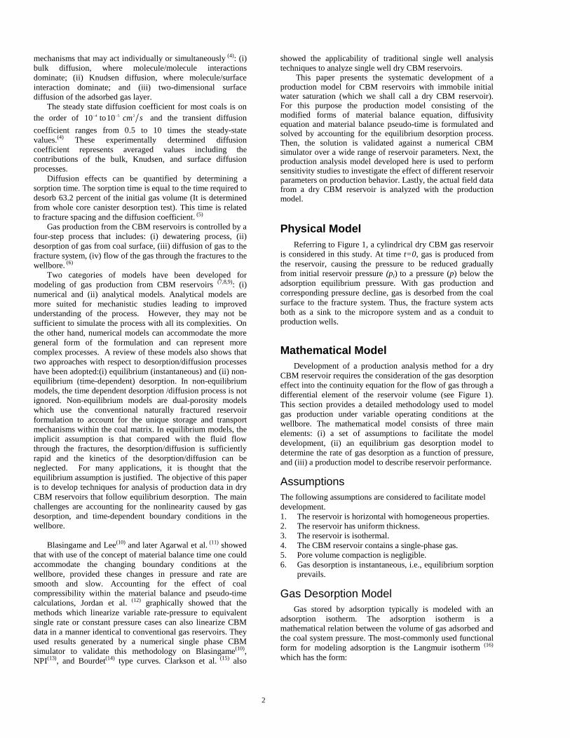
For simulation, the single layer hypothetical reservoir is divided into 20 radially distributed sections. To simulate instantaneous equilibrium, the value of coal desorption time is considered equal to be 0.01 day. To ensure accuracy of the numerical results, we have compared results of two numerical simulators. Figure 3, shows the calculated flowing-wellbore and average-reservoir pressure from GEM-CBM simulator of CMG (25) and Fekete’s numerical CBM simulator (24). A close agreement is observed for case-1 shown in Figure 3 and cases 2 to 6 shown elsewhere (Gerami, 2006) (26).

To examine the validity of the assumption made in the development of the analytical solution presented in this work, we compare the results of the numerical simulator against type-curves developed using the analytical solution. In each case, the calculated pressure, rate and time information are turned to the appropriate pseudo-values as required by the solution developed in this paper. The details of transformations are explained by Gerami (26).

Figure 3(a) shows that the calculated average-reservoir pressure for the constant rate and constant pressure case honor the *Zp material balance equation. Figure 3(b) and 3(d)

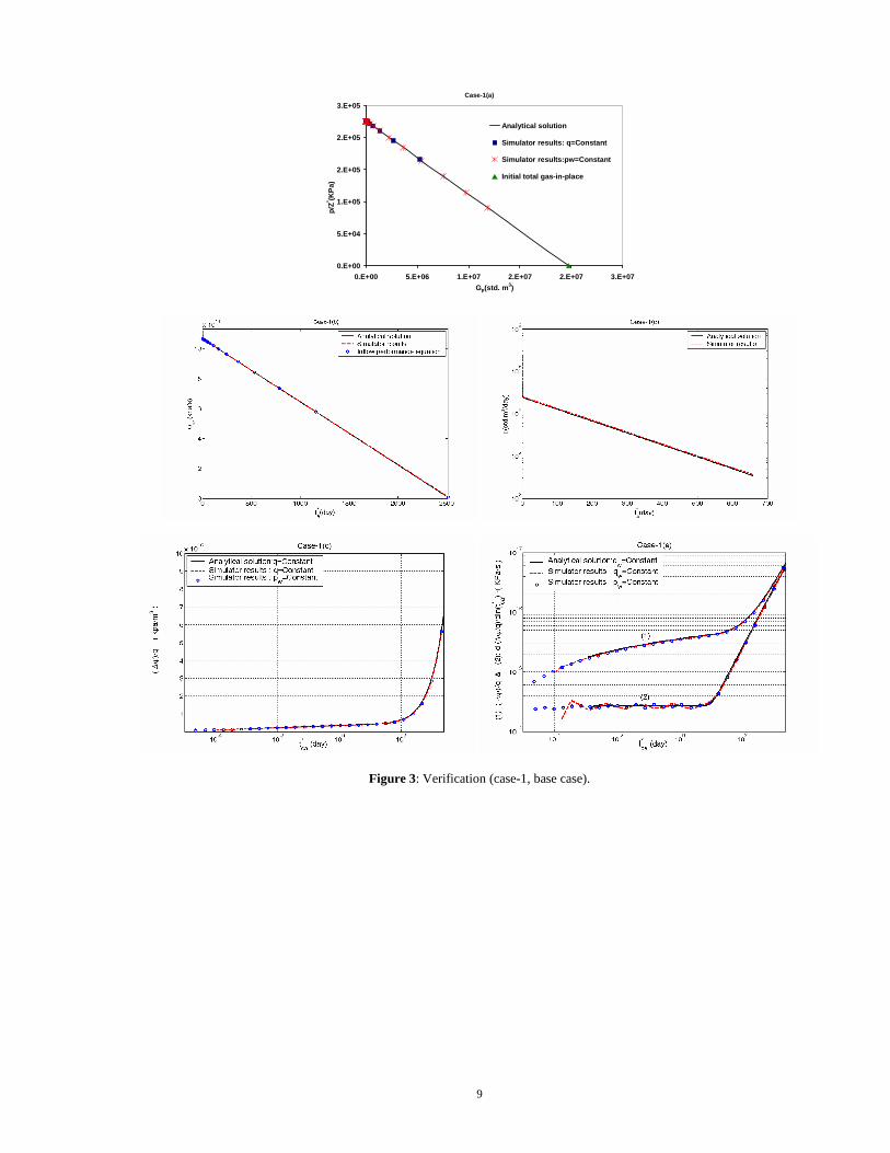
shows that calculated flowing bottomhole pressure agrees with the analytical model during boundary-dominated and infinite-acting flow regime respectively, while Figure 3(c) shows that at a constant bottomhole pressure, production rate exhibits an exponential-decline behavior. Finally, Figure 3(e) shows that the calculated production data for both cases of constant-pressure and constant-rate fall on the analytically calculated pressure-derivative type curve. The agreement is excellent for infinite-acting and boundary-dominated flow regimes. For cases 2 to 6, presented in Figures 4 to 8, we have shown two figures. Those designated by letter (a) show the average reservoir pressure on the *Zp , while those designated by

letter (b) show wellbore flowing pressure and rate. In all cases a close agreement is observed between the analytical and numerical solutions.

In the next section, we use the analytical solution developed here to investigate the effect of some important reservoir operating conditions on gas production from dry CBM reservoirs.

Sensitivity Study Using the analytical model, the effects of Langmuir

pressure, Langmuir volume and wellbore pressure are investigated in this section. For this purpose the hypothetical

5

reservoir described for the base case is used in this study. Unless stated otherwise, the conditions listed in the Table 1 are used as reservoir parameters.

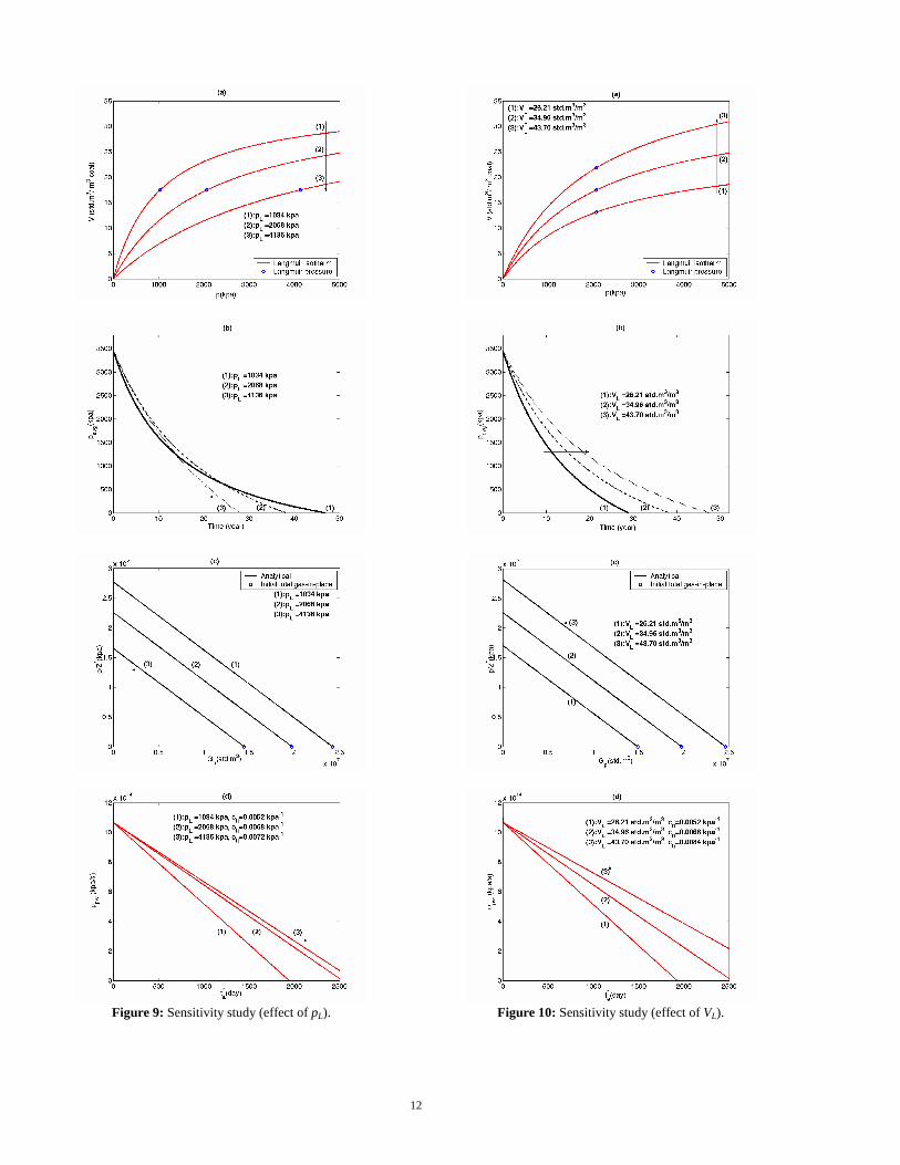
Figures 9 and 10 show the effects of Lp and

LV on the

reservoir and production performance, respectively. As shown in Figure 9(a) the higher the value of

Lp , the lower the gas

content of the coal; consequently the lower the total initial gas-in-place as can be seen from Figure 9(c). In contrast, the higher the value of

LV , the higher the gas content of the coal

and therefore the higher the total initial gas-in-place as can be seen in Figure 10(c). Figures 9(b) and 10(b) show that at early time the effects of

Lp and LV on reservoir pressure can not be

detected, however, at late time their effects become important. Figure 9(b) also shows that the effect of

Lp on reservoir

pressure does not follow a linear trend while that ofLV follows

a linear trend as can be seen from Figures 9(b) and 10(b). Mathematically, Equation (2) shows the cumulative gas desorption is a non-linear function of

Lp and a linear function

ofLV . Figures 9(d) and 10(d) show that as

Lp and LV increase

the flowing wellbore pseudo-pressure increases due to the increase in the total compressibility of gas. Mathematically, from Equations (6) one may notice that the desorption compressibility changes non-linearly with

Lp and linearly

withLV . This is why at high values, the effect of

Lp on flowing

wellbore pseudo-pressure is not as significant as the effect of

LV .

Figures (11) show the effect of wellbore pressure on the rate of gas production when the wellbore pressure reduces from 1725 KPa to 345 KPa. As expected, the lower the wellbore pressure the higher the rate of gas production. However, the effect of wellbore pressure on production rate reduces at low values of wellbore pressure.

Field Case Study In the validation section, we showed how production data

of a dry CBM reservoir (as determined from a simulator) may be analyzed using conventional analysis techniques. A systematic and comprehensive methodology for advanced analysis of conventional production data for determination of hydrocarbon reserve and other reservoir properties (k, S) is given by Mattar and Anderson (27).

In the following, the pressure and rate measurements (variable operating conditions) from a well producing from Horseshoe Canyon coals of the Western Canadian Sedimentary Basin is analyzed (see Table 4 and Figure 12). There has been no or little water production, making this data set suitable for analysis using techniques developed in this paper.

As we shall see, the quality of the data does not allow analysis of the transient data for determination of permeability and skin. However, the analysis of about two years of information shown in Figure 14 indicates that the reservoir shows boundary dominated flow behaviour enabling determination of gas-in-place.

As suggested by Agarwal et al. (11), for noisy production data, it is advantageous to present the dimensionless PTA/RTA

type-curves in the form of

wfiwD

tq

kh

T

p

1 versus

wfi

i

DAQ

21

. They have shown that this would

result in a straight line on Cartesian graph that is anchored at the point 159.021 DAQ provided that the fluid in place

has been estimated correctly. Because the vertical axis,wDp1 ,

is proportional to wfi

tq , one may conclude that the

plot of wfi

tq versus DAQ also converges

at 159.0DAQ . However, the slope of this straight line is

different than that of DAwD Qvsp .1 due to removing khT

from the y-axis expression (wDp1 ).

Using this together with an iterative procedure (27), the estimate of total initial gas-in-place is obtained as 6.36106 std. m3. This value agrees well with other information available in this case. Figure 13 illustrate a match between field data and the theoretical solution.

This analysis is useful when the flow regime is boundary-dominated. Figure 14 shows a log-log graph of normalized pseudo-pressure, q , versus *

cat with its associated

derivative. The derivative plot (open circles) exhibit significant noise, making any analysis of the transient data impossible. However, the boundary dominated flow represented as the unit slope is evident (see solid line). This shows a clear evidence of boundary-dominated flow.

Discussion The production analysis model developed here is based on

the instantaneous desorption of gas from matrix to fracture. According to “Gas Research Institute” (GRI) (28) for the reservoirs that have been commercially developed to date, gas production rates are generally limited by permeability rather than by diffusivity. This means that diffusion has a minor effect on estimates of gas productivity. This condition is true when the time-scale of diffusion in the coal matrix is smaller than the time-scale of Darcy’s flow in the reservoir. In such cases, gas production is limited by Darcy’s flow of gas and the equilibrium approach is adequate for engineering calculations. However, for cases where the diffusion is the limiting process, one needs to consider kinetics of desorption/diffusion between matrix and fracture. For such cases a dual-porosity model is needed (29,30).

The production analysis model developed here assumes no permeability changes as a function of pressure; however, in many CBM reservoirs permeability may be pressure/stress dependent. For reservoirs where this effect is important this model may not be appropriate and a different pseudo-pressure that incorporated pressure dependent permeability can be defined.

Although in our development we did not account for formation compressibility,

fc , for cases that

fc is important

one can simply modify *

tc by adding

fc .

Summary and Conclusion An analytical production model including pressure

transient analysis and production data analysis is developed for the production of gas from a dry CBM reservoir with the instantaneous desorption of gas. Desorption is assumed to follow a Langmuir isotherm. The analytical model is validated against a CBM reservoir simulator with excellent agreement. On the basis of the results presented, the following conclusions are drawn:

6

1. The modified pseudo-time calculated at average reservoir pressure successfully linearizes the modified diffusivity equation.

2. The concept of material balance pseudo-time developed for conventional gas reservoirs can be applied successfully to a dry CBM reservoir with instantaneous desorption provided that the effects of desorption on average reservoir pressure and total compressibility are accounted. For the simple model developed here can therefore be used to analyze the dry CBM production data by all the methods available for production data analysis.

Acknowledgements The authors thank Mrs. Hong for helping in numerical

simulation studies. The study program of Mr. Gerami, a Ph.D. candidate at the University of Calgary, was also supported by a grant from the National Iranian Oil Company (NIOC). This support is gratefully acknowledged.

NOMENCLATURE A Flow area, m2

gB Gas formation volume factor, m3/std.m3

fc Formation compressibility, KPa-1

gc Gas compressibility, KPa-1

dc Desorption compressibility, KPa-1 *

tc Modified total compressibility, KPa-1

h Formation thickness, m

k Absolute permeability, m2 G Initial total gas-in-place, std. m3 Gf Initial free gas-in-place, std. m3 Gp Cumulative gas production, std. m3

gM Molecular weight of methane, Kg/Kmol

p Pressure, KPa p Average reservoir pressure, KPa

bp Optional base pressure, Kpa

pi Initial pressure, KPa pL Langmuir pressure, KPa psc Standard pressure, KPa q Production rate at standard conditions, m3/s

*

dq Desorption rate, Kg/s

*

dq Desorption rate, m3/s

r Radius, m

er Reservoir radius, m

wr Wellbore radius, m

S Laplace parameter t Time, s R Real gas constant, =8.314 KPa. m3/Kmol.K

*

at Modified material balance pseudo-time, s

ct Material balance time, s *

cat Modified pseudo-time, s

T Reservoir temperature, K Tsc Standard temperature, K

gv Gas velocity, m/s

VE Volume of gas adsorbed, m3 gas/m3 coal VL Langmuir Volume, m3 gas/m3 coal

rV Elemental volume, m3

Z Compressibility factor, dimensionless Zi Initial compressibility factor, dimensionless

*Z Modified compressibility factor, dimensionless

*

iZ

Initial modified compressibility factor, dimensionless

Porosity, dimensionless fraction Gas viscosity, KPa.s Radial angle, radian Pseudo-pressure, KPa/s Pseudo-pressure calculated at average reservoir

pressure, KPa/s

i Pseudo-pressure calculated at initial reservoir pressure, KPa/s

wf Pseudo-pressure calculated at flowing wellbore

pressure, KPa/s

REFERENCES 1. GERLING, J., Future Gas Potential: where, what, How

Much; BGR Hanover, 2004 2. MARSH, H., The Determination of Surface Areas of

Coals - Some Physiochemical Considerations; Fuel V. 33, 1965.

3. THIMONS, E. P, and KISSELL, F. N., Diffusion of Methane through Coal; Fuel, pp. 274-280, 1973.

4. SMITH, D.M. and WILLIAMS, F. L., Diffusion Effects in the Recovery of Methane from Coalbeds; Soc. Pet. Eng. J., pp.529-35, Oct.1984.

5. SCHWERER, F.C. et al., Development of Coal-Gas Production Simulators and Mathematical Models for Well-Test Strategies; Gas Research Institute Final Report No. GRI-84/0060, Chicago, Illinois, April, 1984.

6. AHMED, T.H., and MCKINNEY, P.D., Advanced Reservoir Engineering; Elsevier, 2004.

7. KING, G. R. and ERTEKIN, T., State-Of-the-Art Modeling for Unconventional Gas Recovery; SPEFE pp.63-71, March, 1991.

8. KING, G. R. and ERTEKIN, T., State-Of-the-Art Modeling for Unconventional Gas Recovery (Supplement to SPE 18947); SPE 22285: SPEE Book order Dept., Richardson, Texas, 6 pages, 1991.

9. KING, G. R. and ERTEKIN, T., State-of-the-Art Modeling for Unconventional Gas Recovery, Part II: Recent Developments(1989-1994); SPE 29575, presented at the SPE Rocky Mountain Regional/Low-Permeability Reservoirs Symposium held in Denver, CO, U. S.A.,20-22 March 1995.

10. BLASINGAME, T.A. and LEE, W.J., Variable Rate Reservoir Limits Testing; Paper SPE 15028 presented at the Permian Basin Oil and Gas Recovery Conference, Midland, TX, March 1314,1986.

11. AGARWAL, R.G., GARDNER, D.C., KLEINSTEIBER, S.W., and FUSSELl, D.D., Analyzing Well Production Data Using Combined Type Curve and Decline Curve Analysis Concepts; SPE 57916, SPE Reservoir Evaluation and Engineering, October, 1999.

12. JORDAN, C.L., FENNIIAK, M.J., and SMITH, C.R., Case Studies: A Practical Approach to Gas-Production Analysis and Forecasting; SPE 99351, presented at the 2006 SPE Gas Technology Symposium, Calgary, Alberta, Canada, May 15-17, 2006.

13. PALACIO, J.C. and BLASINGAME, T.A., Decline Curve Analysis Using Type Curves Analysis of Gas Well

7

Production Data; paper SPE 25909 presented at the 1993 Joint Rocky Mountain Regional and Low Permeability Reservoirs Symposium, Denver, 26-28 April, 1993.

14. BOURDET, D., AYOUB, J.A., and PICARD, Y.M., Use of Pressure Derivative in Well Test Interpretation; SPE Formation Evaluation, June, 1989.

15. CLRAKSON, C.R., BUSTIN, R.M. and SEIDLE, J.P., Production Data Analysis of Single-Phase (Gas) CBM Wells; SPE 100313, presented at the 2006 SPE Gas Technology Symposium, Calgary, Alberta, Canada, May 15-17, 2006.

16. KING, G. R., ERTEKIN, T., and SCHWERER, F. C., Numerical Simulation of the Transient Behavior of Coal Seam Degasification Wells, SPEFE (April) pp.165-183, 1986.

17. KING, G. R., Material Balance Techniques for Coal Seam and Devonian Shale Gas Reservoirs; SPE 20730, presented at the 65th SPE Annual Technical Conference and Exhibition, New Orleans, Louisiana, September 23-26, 1990.

18. AL-HUSSAINY, R., RAMEY, H.J., and CRAWFORD, P.B., The Flow of Real Gases through Porous Media; JPT, 18, pp.626-636, 1966.

19. LEE, W. JOHN and HOLDITCH, STEPHEN A., Application of Pseudo-time to Buildup Test Analysis of Low-Permeability Gas Wells with Long-Duration Wellbore Storage Distortion; Journal of Petroleum Engineering, pp.2877-2888, December, 1982.

20. BUMB, A. C., and MCKEE, C.R., Gas-Well Testing in the Presence of Desorption for Coalbed Methane and Devonian Shale; SPEFE (March) pp.179-185, 1988.

21. FRAIM, M. L., and WATTENBARGER, R.A., Gas reservoir Decline-Curve Analysis Using Type Curves with Real Gas Pseudopressure and Normalized Time; SPEFE (Dec.) pp.671-682, 1987.

22. SPIVEY J. P. and SEMMELBECK M. E., Forecasting Long-Term Gas Production of Dewatered Coal Seams and Fractured Gas Shales; Paper SPE 29580 presented at the 1995 SPE Rocky Mountain Regional/ Low-Permeability Reservoirs Symposium, Denver Colorado, 20-22 March, 1995.

23. FETKOVICH, M.J., Decline Curve Analysis Using Type-Curves; JPT (June) 1065, 1980.

24. FEKEKETE ASSOCIATES INC., CBM reservoir Simulator; 2006.

25. COMPUTER MODELING GROUP INC., Tutorial: Building, Running, and Analyzing Coalbed Methane Model Using Builder and GEM, 2005.

26. GERAMI, S., Predictive and Production Analysis Models for the Unconventional Gas Reservoirs; Ph.D. Thesis, University of Calgary, 2007.

27. MATTAR, L., and ANDERSON, D.M., A systematic and Comprehensive Methodology for Advanced Analysis of Production Data; Paper SPE 84472, presented at SPE Annual Technical Conference and Exhibition, Denver, Colorado, October 5-8, 2003.

28. GRI, A Guide to Coalbed Methane; Gas research institute, Chapter 3, pp.3.2, Published by Gas Research Institute Chicago, Illinois, U.S.A, 1992.

29. ERTEKIN, T. and SUNG, W., Pressure Transient Analysis of Coal Seams in the Presence of Multi-Mechanistic Flow and Sorption Phenomena; paper SPE 19102 presented at the SPE Gas Technology Symposium, Dallas, TX, June 7-9, 1989.

30. ANBARCI, K. and ERTEKIN, T., A Comprehensive Study of Pressure Transient Analysis with Sorption Phenomena for Single-Phase Gas Flow in Coal Seams; paper SPE 20568 presented at 65th Annual Technical and Exhibition of the Society of Petroleum Engineers, New Orleans, LA, September 23-26,1990.

31. SABET, M.A., Well Test Analysis; Gulf Publishing Company, 1991.

32. CRAFT, B.C and HAWKINS, M.F., Applied Petroleum Reservoir Engineering; Prentice-Hall, 1959.

Table 1: Definition of important variables

Parameter Equation

Pseudo-pressure dpZ

pp

p

pb

2 (7)

Modified pseudo-time

t

ptp

tiia c

dtcpt

0 )()(

**

(9)

Modified total compressibility

dgtccc * (6)

Desorption compressibility 2

Lsc

LLsc

d pppT

ZpTVpc

(8)

Dimensionless radius

w

D r

rr (13)

Dimensionless pseudo-pressure 2*

*

wtii

a

D rc

tkt

(14)

Dimensionless pseudo-pressure

i

sc

sc

D qTp

khT (15)

Dimensionless rate qhkT

Tpq

wfisc

sc

D (16)

Diffusivity equation

D

D

D

D

DD

D

trrr

1

2

2

(17)

Table 2: Solution of Equation (B-9) subjected to different

boundary conditions.(31)

Constant rate solution Infinite-acting reservoir

80908.02

1

DDwDtnt (18)

Laplace space solution, bounded reservoir

SISrKSrISKSS

SrKSrISrISrKS

DeDe

DDeDDe

wD

1111

0101

(19)

Boundary dominated flow- approximate late time

75.02

2

eD

eD

D

DDwrn

r

tt (20)

Constant pressure solution Laplace space solution, bounded reservoir

SrISKSISrKS

SKSrISISrKSq

DeDe

DeDe

D

1001

1111

(21)

8

Table 3(a): Reservoir properties for different cases*

Parameter Case-1 (Base)

q (std. m3/day) (for CR) 1.42x103

pw (KPa) (for CP) 345

T(K) 289

pi(KPa) 3450

Coal density (Kg/m3) 1400

pL(KPa) 2068

VL(std. m3/m3) 34.96

h(m) 3.048

rw(m) 0.0914

re(m) 3048

k(md) 20

0.01

* CR: Constant rate / CP: Constant pressure

Table 3(b): Parameters that change for other cases.

Case-2 Case-3 Case-4 Case-5 Case-6

pi(KPa) pi(KPa) k(md) k(md) pL(KPa)

6895 1378 100 2 3450

Table 4: Case reservoir properties.

T(K) 289

pi(KPa) 1413

Coal density (Kg/m3) 1468

pL(KPa) 4652

VL(std. m3/m3) 13.49

h(m) 8.99

rw(m) 0.0914

0.005

Sw 0.1

rrgg vA

rgg Av

rr r

trp ,

h

wr

trqd ,

q

CBM reservoirh

(a) (b)

Figure 1: Hypothetical radial-cylindrical CBM reservoir.

(a)

0

500

1000

1500

2000

2500

3000

3500

4000

0 1000 2000 3000 4000 5000 6000 7000 8000

Time (day)A

vera

ge r

eser

voir

pre

ssur

e(K

Pa)

GEM-CBMFekete-CBM

(b)

0

500

1000

1500

2000

2500

3000

3500

4000

0 1000 2000 3000 4000 5000 6000 7000 8000

Time (day)

p wf(K

Pa)

GEM-CBMFekete-CBM

Figure 2: Comparison between Fekete Numerical CBM Simulator and GEM-CBM.

9

Case-1(a)

0.E+00

5.E+04

1.E+05

2.E+05

2.E+05

3.E+05

0.E+00 5.E+06 1.E+07 2.E+07 2.E+07 3.E+07

Gp(std. m3)

p/Z

* (KP

a)

Analytical solution

Simulator results: q=Constant

Simulator results:pw=Constant

Initial total gas-in-place

Figure 3: Verification (case-1, base case).

10

0.E+00

5.E+04

1.E+05

2.E+05

2.E+05

3.E+05

3.E+05

0.E+00 5.E+06 1.E+07 2.E+07 2.E+07 3.E+07 3.E+07Gp(std. m3)

p/Z

* (KP

a)

Analytical solution

Simulator results: q=Constant

Simulator results:pw=Constant

Initial total gas-in-place

Case-2(a)

Figure 4: Verification (case-2, pi=1000).

0.E+00

2.E+04

4.E+04

6.E+04

8.E+04

1.E+05

1.E+05

1.E+05

2.E+05

0.E+00 2.E+06 4.E+06 6.E+06 8.E+06 1.E+07 1.E+07 1.E+07Gp(std. m3)

p/Z

* (KP

a)

Analytical solution

Simulator results: q=Constant

Simulator results:pw=Constant

Initial total gas-in-place

Case-3(a)

Figure 5: Verification (case-3, pi=200).

0.E+00

5.E+04

1.E+05

2.E+05

2.E+05

3.E+05

0.E+00 5.E+06 1.E+07 2.E+07 2.E+07 3.E+07Gp(std. m3)

p/Z

* (KP

a)

Analytical solution

Simulator results: q=Constant

Simulator results:pw=Constant

Initial total gas-in-place

Case-4(a)

Figure 6: Verification (case-4, k=100 md).

11

0.E+00

5.E+04

1.E+05

2.E+05

2.E+05

3.E+05

0.E+00 5.E+06 1.E+07 2.E+07 2.E+07 3.E+07Gp(std. m3)

p/Z

* (KP

a)

Analytical solution

Simulator results: q=Constant

Simulator results:pw=Constant

Initial total gas-in-place

Case-5(a)

Figure 7: Verification (case-5, k=2 md).

Case-6(a)

0.E+00

2.E+04

4.E+04

6.E+04

8.E+04

1.E+05

1.E+05

1.E+05

2.E+05

2.E+05

2.E+05

0 2E+06 4E+06 6E+06 8E+06 1E+07 1E+07 1E+07 2E+07 2E+07Gp(std. m3)

p/Z

* (KP

a)

Analytical solution

Simulator results: q=Constant

Simulator results:pw=Constant

Initial total gas-in-place

Figure 8: Verification (case-6, pL=500).

12

Figure 9: Sensitivity study (effect of pL).

Figure 10: Sensitivity study (effect of VL).

13

Figure 11: Sensitivity study (effect of pwf).

0

50

100

150

200

250

300

350

0 100 200 300 400 500 600 700 800

Time (day)

Rat

e(M

SC

FD

)

0

50

100

150

200

250

300

350

Pre

ssu

re(p

sia)

Gas rate Wellbore pressure

Figure 12: Production history for Horseshoe Canyon Coal.

Figure 13: Analysis of Horseshoe Canyon production data- rate cumulative type-curve approach.

Figure 14: Analysis of Horseshoe Canyon production data- derivative analysis approach.

Appendix A: Modified radial diffusivity equation

This appendix presents the derivation of the linearized diffusivity equation for radial flow of gas through a dry CBM reservoir with equilibrium desorption. For the sake of completeness all equations in the main text are mentioned here. As can be seen from Figure 1, it is assumed that the gas control volume consists of a source term which is dependent on the rate of gas desorption from the coal. Under the assumptions described in the main text, the differential form of mass balance on the gas control volume can be expressed as:

gdgrg t

qvrrr

*1 .................................................. (A-1)

where *

dq represents the instantaneous rate of gas desorption

(mass of gas per unit time per unit volume) at time t and radius r due to gas desorption.

Expressing desorption term, *

dq as a function of desorbed

gas volume:

t

Vq dstd

gd* ............................................................................ (A-2)

where std

g and

dV are the gas density and volume of desorbed

gas per unit volume of coal, at standard conditions, respectively. Using the chain rule, *

dq as a function of pressure becomes:

t

p

p

V

RT

Mpq d

sc

gsc

d

* ............................................................. (A-3)

where

LLi

i

Ld pp

p

pp

pVV ........................................................ (A-4)

2L

LLd

pp

Vp

p

V

........................................................................ (A-5)

Introducing Equation (A-5) into Equation (A-3), substituting the resulting equation into Equation (A-1) gives:

tt

p

pp

Vp

RT

Mp

r

vr

rg

L

LL

sc

gscgrg

2

1............... (A-6)

The equation of motion or flux law relates the velocity and pressure gradients within the control volume. Here we use Darcy’s law.

r

pkv

gr

................................................................................. (A-7)

The flow is compressible, from the real gas law

14

Z

p

RT

Mg

g .............................................................................. (A-8)

Substituting Equations (A-8) and (A-7) into Equation (A-6), and assuming constant permeability, Equation (A-6) becomes

t

Z

p

kt

p

pp

Vp

kT

Tp

r

r

p

Z

pr

rL

LL

sc

sc

11

2 ........... (A-9)

Expanding the right hand side of Equation (A-9) and using the definition of gas compressibility given by Equation (A-10), Equation (A-9) can be rewritten as Equation (A-11):

p

Z

Zpc

g

11

.......................................................................... (A-10)

t

p

Z

p

k

c

t

p

ppkT

VTpp

r

p

Z

pr

rrg

Lsc

LLsc

2

1...... (A-11)

The flow of gas in the CBM reservoirs is governed by Equation (A-11). The first term in the left hand side of Equation (A-11) is a flow-dependent term, while the second term is related to the gas desorption rate. The right hand side term shows change in gas storage as a result of change in gas density.

The governing differential equation, Equation (A-11), is non-linear as a result of the strong dependency of gas properties on pressure e.g. Z and , and the existence of the desorption term in this equation. Obviously, the occurrence of this non-linearity is mathematically inconvenient and thus should be eliminated if possible. In an attempt to reduce the non-linearity of Equation (A-11) one may use the Al-Hussainy and Ramey(18) pseudo-pressure function, which is defined as:

dpZ

pp

p

pb

2 ........................................................................ (A-12)

where the base pressure bp is an arbitrary pressure , usually at

the lowest end of the range of pressures of interest during the test. Substituting into Equation (11) and simplifying, Equation (A-11) is converted into Equation (13) as:

t

cckr

rrr dg

1

.......................................... (A-13)

Equation (A-13) contains an additional compressibility term which is called desorption compressibility,

dc , by Bumb and

Mckee. (19) Desorption compressibility in Equation (A-13) is expressed as:

2Lsc

LLsc

d pppT

ZpTVpc

.................................................................. (A-14)

Modifying the traditional definition of total compressibility, Equation (A-14) may be written as:

dgtccc * .................................................................................. (A-15)

Now the diffusivity equation for CBM methane is defined as:

tk

c

rr

rrtrt

t

,

*1

.............................................. (A-16)

Equation (A-16) is non-linear because the product trt

c,

* is a

strong function of pressure and thus ofp

. To complete the

linearization, modified pseudo-time, *

at , is defined as:

t

pt

tiia c

dtcpt

0

*

**

................................................................ (A-17)

where pt

c* is the product of viscosity and total

compressibility calculated at average reservoir pressure. In the definition of the modified pseudo-time it is assumed

that the product trt

c,

* as a function of time and space is

accurately replaced by the product pt

c* which is only a

function of average reservoir pressure and therefore, time. Using the chain rule and definition of pseudo-time, Equation (A-17), one can obtain Equation (A-18) as:

a

tiiptp tc

tc

**

)()(............................................................ (A-18)

The diffusivity equation can be linearized if the product of total compressibility and viscosity in the right hand side of Equation (A-16) could be approximated by

ptc* ( *

tc at average

reservoir pressure). By making this assumption, we may write:

*

*1

a

tii

tk

c

rr

rr

.................................................... (A-19)

Equation (A-19) is linear; there is hope that solutions to the linear equation describing flow of a slightly compressible liquid can be used rigorously for dry CBM reservoirs.

Using pseudo-time requires the knowledge about how the reservoir pressure varies with time. The reservoir pressure can be obtained from the modified material balance equation, Equation (3).

Appendix B: Material-Balance Pseudo-Time for Dry CBM Reservoirs with Equilibrium Desorption.

To obtain the material balance pseudo-time for a dry CBM reservoir one may modify the gas reservoir material balance pseudo-time by accounting for desorption of gas from the coal matrix. For this purpose one may use the modified material balance equation for CBM reservoirs (17).

15

G

GG

Z

p

Z

p p

i

i

**................................................................... (B-1)

where

scL

Lsc

Tpp

ZVTp

ZZ

1

* ............................................................ (B-2)

To develop the material balance pseudo-time for a dry CBM the Equation (B-1) must be reformulated in terms of pseudo-pressure, Equation (B-3), and time.

dpZ

pp

p

pb

2 .......................................................................... (B-3)

To accomplish reformulation, we use the chain rule as seen in Equation (B-4) below:

dt

d

d

pd

Z

p

dp

d

Z

p

dt

d

**.............................................. (B-4)

Re-arranging Equation (B-4) yields Equation (B-5):

*

*

Z

p

dp

d

dp

d

Z

p

dt

d

dt

d

................................................................ (B-5)

The first derivative in the numerator and the derivative in the denominator of Equation (B-5) are simply the derivative of Equation (B-1) with respect to time and pressure, respectively. The second derivative in the numerator of Equation (B-5) is simply the derivative of Equation (B-3) with respect to pressure. Taking the derivatives and Combining the resulting equations, we get Equation (B-6).

scL

Lsc

fi

i

Tpp

ZTVp

p

Z

Zp

tq

GZ

p

dt

d

111

2

*

*

................................ (B-6)

From Equation (B-2), pZ * in terms of fluid and reservoir

properties can be expressed as:

2

*

1

11

scL

Lsc

scL

Lsc

scL

Lsc

Tpp

ZTVp

Tpp

ZTVp

pZ

Tpp

ZTVp

p

Z

p

Z

................. (B-7)

Taking derivatives and substituting the result into Equation (B-6), gives:

*

2

t

fi

i

c

tq

GZ

p

dt

d

..................................................................... (B-8)

where *

tc is the modified total compressibility factor which is

given by Equation (B-9).

2

* 11

Lsc

LLsc

t pppT

ZpTVp

p

Z

Zpc

...................................... (B-9)

Substituting gc (Equation (A-10)) and dc (Equation (A-14))

into Equation (B-9), *

tc becomes:

dgtccc * .................................................................................. (B-10)

For the case of conventional gas reservoir, LV is zero and *

tc

becomes equal tog

c . Equation (B-1) assumes that the formation

compressibility is negligible. Integrating Equation (B-8) within the appropriate limits and dividing the result by tqw

, we get:

dtc

q

tqGZ

p

tq

t

ti

ii

0

**

2

...................................................... (B-11)

Now we will define the modified material balance pseudo-time, *

cat , as seen below in Equation (B-12).

dtc

tq

tq

ct

t

t

iti

ca 0

*

*

*

...................................................................... (B-12)

Combining Equations (B-11) and (B-12), Equation (B-13) is obtained.

*

**

2ca

iiti

ii tGZc

p

q

................................................................ (B-13)

From Equation (B-13) one may notice that in the case of constant rate production the material balance pseudo-time becomes equal to pseudo-time, i.e. **

acatt .

Appendix C: Deliverability Equation (Inflow Performance Equation)

After pseudo-steady state has been reached, the entire drainage area of the well is gradually emptied. During pseudo-steady state the pressure transients affect the entire drainage area of the well. Then, if

wf declines by , the pseudo-

pressure declines by throughout the drainage area of the well, which means that the average pseudo-pressure in drainage area, , also declines by . Accordingly during pseudo-steady state the following condition must hold:

wf

Constant ........................................................................ (C-1)

16

From Equation (B-13) which is a material balance equation, we also have

*

**

2ca

iiti

ii tGZc

p

q

.................................................................. (C-2)

Measurement of p and therefore determination of is impractical during the normal operation of a field. Therefore, to complete the formulation of Equation (C-2), we have to find a relation between and

wf . For this purpose, we apply

Darcy’s law to radial flow and then find the volumetric pseudo-average pressure . In the case of pseudo-steady state flow from Equation (C-2) we could write

*

*22

2cai

iitiwe

gi dt

d

p

ZchrrqB

............................................. (C-3)

It must be noted that the term GZi

* in Equation (B-13) is replaced

byfi

GZ (this equality can be easily obtained from the definition of the

modified material balance equation and the modified compressibility factor). Instead of evaluating the flow rate at the wellbore ( q ), one can write Equation (C-3) at any radius ( r ) as given by Equation (C-4).

*

*22

2cai

iitie

gir dt

d

p

ZchrrBq

............................................ (C-4)

Assuming 22

ewrr , Equation (C-4) is divided by Equation (C-

3) and is solved for rq in terms of q gives:

2

2

1e

r r

rqq .............................................................................. (C-5)

Substituting Equation (C-5) into Darcy’s law, one obtains:

dr

dprhkB

r

rq g

e2

12

2

.......................................................... (C-6)

Using the definition of pseudo-pressure andg

B , Equation (C-6)

becomes:

wf

e

w

dkhTp

T

r

dr

r

rq

sc

sc

r

r e

2

2

1 ................................................... (C-7)

Assuming 2ew

rr is very small, the pressure at a given radius

becomes:

2

2

2ln

ewsc

sc

wf r

r

r

r

khT

Tqp

............................................. (C-8)

Volumetric average pseudo-pressure for a radial system may be expressed by the integral

22

22

e

r

r

e

r

r

r

rdr

hr

drrh

V

dV

e

w

e

w

................................ (C-9)

Substituting from Equation (D-8) gives:

2

2

2

2ln2

e

r

r ewsc

sc

wf

r

rdrr

r

r

r

khT

Tpqe

w

........................... (C-10)

Integrating between limits:

4

3ln

w

e

sc

sc

wfr

r

khT

Tpq

............................................... (C-11)

Similar analysis for oil reservoir is given by Craft and Hawkins

(32). Equation (C-11) is the pseudo-steady state solution on the

basis of the “constant rate equation”. Combining pseudo-steady state Equation (C-11), and the modified material balance equation, Equation (C-2), gives:

*

*

24

3ln

ca

fiiti

iw

e

sc

sc

wfi

tGZc

p

q

r

r

khT

Tpq

...................... (C-12)

Therefore the final form of pseudo-steady state equation for the flow of gas in a dry CBM reservoir becomes:

4

3ln

2 *

**

w

e

sc

sc

ca

iiti

iwfi

r

r

khT

Tpt

GZc

p

q

...................... (C-13)

Because Equation (C-13) is expressed in term of the modified material balance pseudo-time, it is applicable to both constant production and constant pressure wellbore condition. From Equation (C-13) one can determine G i.e., the reservoir gas-in-place. If the well is indeed producing in pseudo-steady state flow regime, then a plot of qq

wfi versus the

modified material balance pseudo-time *

cat yields a straight line.

From the slope of the straight line,GZc

p

iiti

i

**

2

,it is possible to

determine G . As mentioned earlier the importance of using material

balance time is the conversion of the constant pressure solution into the widely used constant rate solution. On this basis, Equation (20) (see Table 2) is applicable for both of the constant pressure and constant rate production conditions provided that the modified material balance pseudo-time is used in the calculations. Equation (20) in dimensional form may be written as:

75.0

22

*

w

e

etii

ca

sc

scwfi

r

rn

rc

kt

khT

Tp

q

...................... (C-14)

17

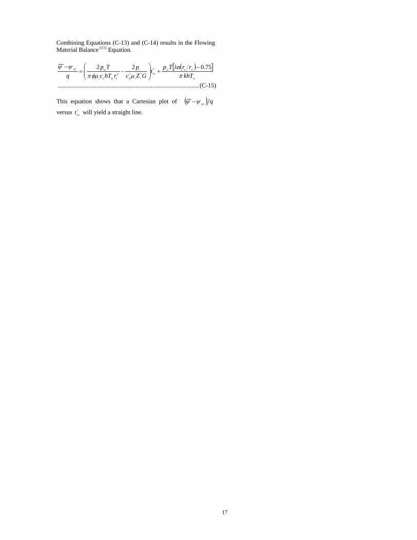
Combining Equations (C-13) and (C-14) results in the Flowing Material Balance (11) Equation.

sc

wesc

ca

iiti

i

esctii

scwf

khT

rrnTpt

GZc

p

rhTc

Tp

q 75.022 *

**2

........................................................................................... (C-15)

This equation shows that a Cartesian plot of qwf

versus *

cat will yield a straight line.