Título artículo / Títol article:

Two-stage procedure based on smoothed ensembles

of neural networks applied to weed detection in

orange groves

Autores / Autors

Torres-Sospedra, Joaquín ; Nebot Roglá, Patricio

Revista:

Biosystems Engineering Vol. 123, 2014

Versión / Versió:

Preprint del autor

Cita bibliográfica / Cita

bibliogràfica (ISO 690):

TORRES-SOSPEDRA, Joaquín; NEBOT, Patricio. Two-stage procedure based on smoothed ensembles of neural networks applied to weed detection in orange groves. Biosystems Engineering, 2014, vol. 123, p. 40-55.

url Repositori UJI:

http://hdl.handle.net/10234/123543

1

Two-Stage Procedure Based on Smoothed Ensembles of Neural Networks applied to Weed Detection in Orange

Groves

Joaquín Torres-Sospedraa,1

and Patricio Nebotb

a Geospatial Technologies Research Group, Institute of New Imaging Technologies, Universitat Jaume I, Castellón, Spain. Joaquin.Torres@uji.es

b Biofísica y Física Médica, Dpto. Fisiología, Facultat de Medicina i Odontología, Universitat de Valencia, Valencia, Spain. Patricio.Nebot@uv.es

1 Corresponding author: phone:+34 964 38 7686 email: Joaquin.Torres@uji.es

ABSTRACT

The potential impacts of herbicide uti lisation compel producers to use new methods of weed control. The problem of how to reduce the amount of herbicide and yet

maintain crop production has stimulated many researchers to study selective herbicide application. The key of selective herbicide application is how to discriminate the weed areas efficiently. We introduce a procedure for weed

detection in orange groves which consists of two different stages. In the first stage, the main features in an image of the grove are determined (Trees, Trunks, Soil and

Sky). In the second, the weeds are detected only in those areas which were determined as Soil in the first stage. Due to the characteristics of weed detection (changing weather and light conditions), we introduce a new training procedure

with noisy patterns for ensembles of neural networks. In the experiments, a comparison of the new noisy learning was successfully performed with a set of well

known classification problems from the machine learning respository published by the University of California, Irvine. This first comparison was performed to determine the general behavior and performance of the noisy ensembles. Then,

the new noisy ensembles were applied to images from orange groves to determine where weeds are located using the proposed two-stage procedure. Main results of

this contribution show that the proposed system is suitable for weed detection in orange, and similar, groves.

Keywords: Agricultural Robotics, Agricultural Sensing, Terrain Classification

1 Introduction

According to armers we interviewed, weed control is an expensive and

time-consuming activity in agriculture. Moreover, long-term use of herbicides could damage people, animals and the environment. Unfortunately, agricultural

herbicides and fertilisers have been uniformly sprayed in fields and overused in conventional practice. This has caused severe environmental pollution of high levels of Phosphate, Potassium or Nitrogen in groves and aquifers (Stayte &

Vaughan, 2000). Therefore, efforts are being encouraged in designing weed-detecting technologies for precision spraying with selective herbicides in

order to save herbicides and reduce environmental pollution without sacrificing

2

crop yields (Moshou, Vrindts, Ketelaere, Baerdemaeker, & Ramon, 2001; Burks, Shearer, Heath, & Donohue, 2005; Cho, Lee, & Jeong, 2002; Bossu, Gee, & Truchetet, 2008). Our intention is to create a weed detection system and integrate it

into an autonomous robotic system such as the ATRV-2 we described in Nebot, Torres-Sospedra, and Martínez (2011).

The automatic detection of weed areas in orange groves has not been widely studied. However, there is a vast literature on weed/crop discrimination. In orange groves, there can be color similarities among weed areas and orange tree leaves

so a direct detection based only on color can not be performed. Moreover, some important aspects such as weather or light conditions should be considered. For

this reason, a two-stage system is introduced in this paper to detect weeds in groves where a robotic system can navigate through. This research is focused on orange groves due to its importance on the economy of western Spain. In the first

stage, the main areas of a capture (e.g, soil) are determined. Later, in the second stage, weeds are detected on soil areas.

To perform the classification tasks we use ensembles of Multilayer Feedforward Networks (also known as MF net, Multilayer Perceptron or MLP network). The performance of MLP networks can be improved by using a committee formed by

several networks (see Tumer & Ghosh, 1996; Dietterich, 2000; Bishop, 2006)]. Using artificial neural networks to detect weeds is not new. Sung, Kwak, and Lyou

(2010) and Moshou et al. (2001) found that this network provided good classification rates for terrain classification and weed detection in different contexts. Moshou et al. (2001) used a MLP network for classification of reflectance spectra

from crop and weeds using a spectrophotometer. Burks et al. (2005) used an Artificial Neural Network (ANN) to distinguish among six species of weeds and detect their presence in raw images which covered approximately a ground area of

0.23 x 0.3 m. Cho, Lee, and Jeong (2002) also used an ANN for weed-plant discrimination using images captured in zenital/overhead view. Cruz-Ramirez,

Hervás-Martínez, Jurado-Expósito, and López-Granados (2012) also introduced an ANN-based model cover crop identification.

Other methods have also been used to perform weed detection. In Bossu, Gee,

and Truchetet (2008) machine vision techniques were applied to discriminate between crops and weed using the captures of a monochrome CCD camera.

Specifically, they applied image processing based on spatial information using a Gabor filter. Asif, Amir, Israr, and Faraz (2010) introduced a vision system for autonomous weed detection robot. This system enabled the navigation of the

robotic system between the inter-row spaces of crop for automatic weed control but a direct weed detection was not introduced. Similar research was introduced in

Tellaeche, Burgos-Artizzu, Pajares, and Ribeiro (2007) and Tellaeche, Pajares, Burgos-Artizzu, and Ribeiro (2011) where the weed detection consisted of two sub-processes: image segmentation and decision making with Support Vector

Machines and Bayesian/Fuzzy k-Means Paradigms.

The main difference of the proposed system with respect to previous systems is

that it relies on two ensembles of MLP networks, the first one for terrain-based classification and the second one for detecting weeds on soil. The weed detector is able to detect weeds on soil instead of discriminate crop and weeds. In this way,

other elements such as leaves, fallen fruits and trash are automatically rejected. This system can be implemented into an autonomous computer-assisted robotic

system, such as the ATRV-2. Finally, a new training algorithm with noise is applied

3

to the two stage system, due to promising preliminar tests we have previously obtained in other classification contexts.

2 Material and Methods

The here proposed classification system for weed detection is divided into two

stages. In the first one, the main elements of the image (orange grove) are determined. In the second one, weed detection is done on those parts of the image which correspondes to Soil according to the first classification (terrain

classification) because weeds are located on soil. Both tasks are perfomed by means of an advanced classifier based on noisy ensembles of neural networks. A

visual representation of the whole system is shown in Fig. 1.

This weed detector was designed to be integrated into an autonomous robotic system, specifically an ATRV-2 vehicle, whose vision system consists of a VGA

camera (640x480 pixels). A manual calibration procedure, repeated in each grove, with visual marks was done. With this calibration, the distance (depth and lateral

displacement) with respect the robotic system was approximated. This approximation was accurate enough for close and medium-distance weed areas, even for a grove with semi-irregular ground (see Table 2).

In each stage, the corresponding features were extracted from the captured images and they were then processed by a classification system based on ensembles of

neural networks generated with the Noisy Learning procedure.

This section is introduced as follows. First, the concepts related to the base classifier systems (neural networks) and ensembles are introduced. Second the

new noisy learning is fully described. Then the general experiments for comparison purposes are detailed. Finally, the proposed two stage system and the classifiers used in the two stages are fully described.

2.1 General Ensemble-Based Classification

2.1.1 Neural Networks theorerical background

The MLP network is the architecture used in the experiments carried out in this paper with ensembles. This is a feed-forward neural network with an architecture

that closely resembles the -Perceptron proposed by Rosenblatt in 1961 and the

layered machine proposed by Nielson in 1965 as described in Pao (1989).

This network architecture was selected because it is widely known (see Ripley, 1996; Bishop, 2006) and has also been used for weed detection (Moshou et al.,

2001; Cho et al., 2002; Burks et al., 2005). Moreover, the comparative studies carried out in Torres-Sospedra (2011) showed that this network could be used for weed classification and the computational costs were reasonable.

In this study, the original datasets were divided into three different subsets to perform the training and evaluation tasks. The first set was the training set (T)

which was used to adapt the weights of the networks using the Backpropagation (Backward Propagation) algorithm (Rumelhart & McClelland, 1986; Rumelhart, Hinton, & Williams, 1988). The second set was va lidation set (V) which was used to

select the final network configuration. This validation set was used to avoid overfitting during training. Then, the test set (TS) was used to obtain the accuracy

4

of the network. Finally, the learning set (L) is the union of of T and V.

2.1.2 Ensemble methods

An ensemble of neural networks is a collection of finite different networks that solve the same classification problem. According to the literature (Tumer & Ghosh, 1996;

Bishop, 2006), the ensemble approach is quite interesting because diversity is increased, and therefore the error in classification decreases, as new independent neural networks are added to the ensemble.

The networks of an ensemble are most useful when they make independent errors (Tumer & Ghosh, 1996; Dietterich, 2000). Although there are several ways to

generate ensembles, one of the most important is based on using different learning sets according to previous experiments (Torres-Sospedra, 2011). Diversity is provided by the fact that the training and validation sets are different for each

network of the ensemble.

There are many ensemble models that are suitable for classification. For this

reason, we selected the following four models for a first evaluation of the noisy learning: Simple Ensemble, Bagging, CVCv3WCB and CVCv3Conserboost. Simple Ensemble was included because it is the easiest way to generate an

ensemble. CVCv3Conserboost and CVCv3WCB are both ensembles based on Cross-Validation Boosting, but they are distinct from each other and both provide

good classification results in general cases according to Torres-Sospedra (2011). Bagging was selected because it is a well-known model and there is a variant in the literature in which noise was introduced (Raviv & Intratorr, 1996).

The Output Average was selected to fuse the information of the networks. This is a simple but effective combiner according to previous experiments (see Torres-Sospedra, 2011). Moreover, the Boosting Combiner (see Kuncheva &

Whitaker, 2002) was used for CVCv3WCB and CVCv3Conserboost.

2.2 Adding special noise to the input values

Terrain based classification and Weed detection are open classification problems, e.g. brightness of weed areas can be differ depending on the grove or, even in the

same grove, brightness can vary depending on weather. Considering all the possible scenarios for both problems is nearly impossible, therefore a learning

procedure should be used. In particular, we propose a new noisy learning for MLP networks and ensembles in which the patterns used to train the neural network are modified by adding a special noise in each epoch. For Terrain-based classification

and Weed detection, the machine learning synonims pattern and sample correspond to the information from the capture which is being processed by the

classifier system (detailed in Section 2.4).

On the one hand, this learning uses different training samples, so more scenarios for classification are considered, that is, slightly different weeds areas are

considered. On the other hand, diversity of the ensemble system is increased due to the use of slightly different samples and training sequences.

However, we do not intend to inject disproportional or arbitrary noise, such as Bagging with Noise (Raviv & Intratorr, 1996) and Observational Learning Algorithm

5

(Jang & Cho, 1999), because the injection of arbitrary noise could even decrease the classification performance (Torres-Sospedra, 2011). So, we introduce a noisy learning procedure along with a procedure to restrict the values of the injected

noise vector. In our algorithm, the maximum distance allowed for a new noisy pattern is proportional to the Euclidean distance from the original pattern to the new

noisy pattern. This proportion factor is obtained by using a case-based parameter, , which should be empirically determined for each classification task. For the

weed detection problem, this value is also valid for other groves with similar weed species and distribution.

First the description of this new learning procedure is introduced in Algorithm 1.

Then, we detail the initialisation phase and the procedure to add noise.

2.2.1 Learning procedure with noise

The new learning procedure is similar to the original Backpropagation, with the differences indicated in Algorithm 1. The target equation which is minimized and the equations used to adapt the networks are the same. However, the original

Backpropagation was modified to include noise. These modifications were done at the beginning of the procedure and in each iteration of the training algorithm.

The process to generate the random noise was divided in two steps. In the first step, some required variables used to generate the random noise were initialized. In the second step, performed in each iteration of the learning procedure, random

noise was added to each training sample (pattern from T).

Algorithm 1. Noisy MF Network Training { T , V }

Set initial weights randomly

Calculate distance to closest neighbor vector: 𝒅 ∀𝒙 ∈ 𝑻

Set maximum distance to noisy pattern: 𝒎𝒅 ∀𝒙 ∈ 𝑻

Initialize index vector: : 𝒊𝒏𝒅𝒆𝒙 = {𝟏, … , 𝑵𝒑𝒂𝒕𝒕𝒆𝒓𝒏𝒔 }

for 𝒆 = 𝟏 to 𝑵𝒆𝒑𝒐𝒄𝒉𝒔 do

Randomly reorder the index vector: create index

for 𝒊 = 𝟏 to 𝑵𝒑𝒂𝒕𝒕𝒆𝒓𝒏𝒔 do

Select sample 𝒙𝒊𝒏𝒅𝒆𝒙(𝒊) from 𝑻

Generate vector 𝒓𝒂𝒏𝒅𝒐𝒎𝒏𝒐𝒊𝒔𝒆

Randomly generate a n-dimensional vector: randomvector

Normalize vector: randomdirection

Set vector’s final length: randomnoise

Set noisy pattern: 𝒏𝒙𝒊 = 𝒙𝒊𝒏𝒅𝒆𝒙(𝒊) + 𝒓𝒂𝒏𝒅𝒐𝒎𝒏𝒐𝒊𝒔𝒆

Adjust the trainable parameters with 𝒏𝒙𝒊

end for

Calculate 𝑴𝑺𝑬 over validation set 𝑽

Save epoch weights and calculated 𝑴𝑺𝑬

end for

Select epoch with lowest MSE on validation set and assign its weights to the final network

Save network configuration

Symbol represent the new lines introduced to the original Backpropagation algorithm.

6

Note that the training algorithm is an iterative procedure in which an iteration corresponds to an epoch. In each epoch, all the patterns from the training set were iteratively used to adapt the network in a random order. Before adapting the

weights, the random noise vector was generated and injected to the original pattern. Once the network was updated with all the noisy patterns from the training

set, the network error (as Mean Squared Error) in the epoch was tested on the independent validation set. Finally, the network configuration (weights) corresponded to the configuration of the epoch with lowest validation error.

2.2.2 Initialisation phase

In the new training algorithm, some initial steps were carried out as follows:

• Set initial weight values.

• Calculate distances to nearest neighbor.

• Set maximum distance to noisy pattern.

Firstly, the initial weight values of the neural network were randomly set. These

weights were different for each network in order to increase diversity. If all the networks share the same initial configuration then the probability of arriving to the same final configuration will be higher.

Secondly, the Euclidean distance to the closest neighbor was calculated for each sample or pattern of the training set T. With this procedure, a new vector, d, is

generated with the corresponding distances. As an example, di refers to the Euclidean distance between pattern xi and its nearest neighbor. A graphical example is shown in Fig. 2.

In Fig. 2, it has been supposed the small training set with four two-dimensional patterns of a simple classification problem where the number of inputs is two (represented by the horizontal and vertical positions of the pattern in the graphics).

Although it is not realistic, it shows how noise is injected. In the left part these patterns are represented with different shapes: Circle, Triangle, Star and Square.

We can see that the Circle is not close to the other ones and the other three are quite close to each other. In the right illustration, we denote with an arrow the distance to the closest neighbor for each individual pattern, di. In the example, d1

corresponds to the Circle, d2 corresponds to the Triangle, d3 corresponds to the Star and, finally, d4 corresponds to the Square.

Then, the maximum distance to a noisy pattern was calculated for each pattern x1, defined as the largest distance between the pattern and the new noisy pattern based on it. This distance, mdi in Eq. (1), depends on the distance vector di

(calculated in the previous step) and the case dependent parameter .

𝑚𝑑𝑖 = 𝛼 · 𝑑𝑖 , 𝛼 ≥ 0 (1)

Fig. 3 shows three graphical examples of the area in the input feature space in

which the noisy patterns can be located. As previously mentioned, the input feature space of the image is two-dimensional but it is greater for terrain classification and weed detection. These areas are shown as a light circle centered in each pattern.

For instance, any noisy pattern based on the first pattern (Black Circle) will be located in the gray area. Each example represents a different value of : A value

close to 0, a value close to 1 and a value higher than 1. In the experiments, the

7

value of has been empirically set with the constraint that its values should be in

range [0.1,…,0.9] to avoid null noise (=0), insignificant noise (≈0) and the

inherited problems of high noise (>1).

2.2.3 Adding noise phase

Noisy training, as Backpropagation, is an iterative procedure which is repeated for

a prefixed number of epochs where the following steps are performed:

• Reordering patterns.

• Generate noise vectors.

• Adapt the networks with noisy samples.

Firstly, the sequence of patterns was randomly reordered. The performance of the

ensemble is expected to be improved when this dynamic reordering is used because the gradient descend minimisation is not overfitted with the same sequence of patterns (Torres-Sospedra, 2011). The index(i) was introduced to link

the reordered and original training sets, e.g. index(1) corresponds to value 2 in Fig. 5 (right) because the first pattern of the reordered training set (the Triangle) was

originally the second pattern.

The reordered training set was used to adapt the trainable parameters. For each pattern from the reordered training set (denoted with index i), a normalized random

vector was generated to represent the direction and sense of the noise to be injected. This new vector was denoted with randomdirectioni and is introduced in

Eq. (2):

𝑟𝑎𝑛𝑑𝑜𝑚𝑑𝑖𝑟𝑒𝑐𝑡𝑖𝑜𝑛𝑖 =𝑟𝑎𝑛𝑑𝑜𝑚𝑣𝑒𝑐𝑡𝑜𝑟𝑖

𝑚𝑜𝑑𝑢𝑙𝑢𝑠 (𝑟𝑎𝑛𝑑𝑜𝑚𝑣𝑒𝑐𝑡𝑜𝑟𝑖 ) (2)

where randomvectori is a vector that contains n random values and each value is unformly distributed in [-1,…,1]. The number of elements, n, corresponds to the

number of features (input values) of the problem. In the example shown in the figures, each pattern is represented with only two features and n is equal to 2. The randomvector was divided by its modulus in order to obtain a unitary vector;

however, the randomdirection vector does not accomplish the requirements related to the maximum distance (its modulus is 1). For this reason, the final length of the

noise vector, randomnoisei, was set according to Eq.(3):

𝑟𝑎𝑛𝑑𝑜𝑚𝑛𝑜𝑖𝑠𝑒𝑖 = 𝑟𝑎𝑛𝑑𝑜𝑚𝑣𝑎𝑙𝑢𝑒 · 𝑚𝑑𝑖𝑛𝑑𝑒𝑥 (𝑖) · 𝑛𝑜𝑖𝑠𝑒𝑑𝑖𝑟𝑒𝑐𝑡𝑖𝑜𝑛𝑖 (3)

To set the vector’s length, noisedirectioni was multiplied by the maximum distance

allowed for the pattern (mdindex(i)) and a random factor uniformly distributed in [0,…,1]. With this procedure, the modulus of the final noise vector is equal to or less

than the maximum distance allowed. Note that the maximum distance for the i-th pattern does not correspond to mdi because the training set was reordered, so mdindex(i) must be used instead. Moreover, the random value provides the relative

length of the vector with respect to the maximum distance.

Finally, the noisy pattern was generated according to Eq. (4). and was used to

adapt the trainable parameters (weights of the networks) as in Backpropagation. The target and the equations used to adapt the weights were not modified.

𝑛𝑥𝑖 = 𝑥𝑖 + 𝑟𝑎𝑛𝑑𝑜𝑚𝑛𝑜𝑖𝑠𝑒𝑖 (4)

8

A graphical description of how a noisy pattern is generated can be found in Fig. 4. This figure introduces how randomvector, randomdirection and randomnoise are generated using a simple 2D example. Finally, the figure also illustrates how the

noise is injected over the pattern.

Fig. 5 shows the original training set along with the areas in which the noisy

patterns can be located. In addition, three examples of specific training set in three different epochs are shown. Note that the order in which the noisy patterns are picked from the training set differs in the three examples.

2.3 Evaluation of the new ensemble model

The ensembles were evaluated on an heterogeneous set of classification problems to test the viability of the proposed Noisy Learning. In particular, ensembles of 3, 9, 20 and 40 networks were built according to the four selected ensembles using the

two training algorithms (Backpropagation and noisy learning). Nineteen classification problems of the University of California at Irvine (UCI) repository

(Asuncion & Newman, 2007) with optimal training parameters were used to test the ensembe models (Table 1). To apply the noisy learning to these ensembles, the networks were trained using the learning procedure described in Algorithm 1

instead of the original Backpropagation.

The training parameters were set after performing a trial-and-error procedure with

cross-validation. First, we tested the accuracy of the MLP network with different hidden values (ranging from 2 to 40) and standard step/momentum values (0.1 and 0.01). Then, we have selected the number of hidden nodes which provided the best

performance on the validation set (V). Finally, we carried out a fine grid search to find the best step and momentum values.

We did not fix the number of inputs and outputs because they correspond, respectively, to the features and classes of the original classification problem. The number of patterns corresponds to the total number of patterns of the database

used in the experiments. The databases were divided into three sets as mentioned in Section 2.1.1. The training set, T, contained 64% of samples from the original

dataset, whereas the validation and test sets contained 16% and 20% of the patterns, respectively.

A similar procedure was used to set the parameter of the noisy learning, , for each

dataset. In particular, a fine grid search was carried out in range [0.1,…,0.9] and the values which report the lowest error in the V were used.

The success of the proposed methodology was evaluated by comparing the general performance of the ensembles with the traditional learning procedure and

noisy alternative. The mean Percentage of Error Reduction across all datasets (mean PER) was used to calculate how the error has been reduced with respect to a base classifier (the single MLP network in this case) and was used to compare

ensembles. Individual PER values, Eq.(5), ranges from 0%, where the ensemble and the single network provide the same classification rate (percentage of correctly

classified patterns), to 100%, where the ensemble provides a classification rate of 100% and the error has been totally reduced. It can also yield negative values, which mean that the ensemble provides a lower classification rate than the single

network.

9

𝑃𝐸𝑅 = 100 ·𝑃𝑒𝑟𝑓𝑒𝑛𝑠𝑒𝑚𝑏𝑙𝑒 −𝑃𝑒𝑟𝑓𝑠𝑖𝑛𝑔𝑙𝑒𝑛𝑒𝑡

100 −𝑃𝑒𝑟𝑓𝑠𝑖𝑛𝑔𝑙𝑒𝑛𝑒𝑡 (5)

where Perf is the classification rate (percentage of correctly classified patterns) for the ensemble and the single network.

The Two-tailed Student's T-Test for Paired Samples was used to provide a

statistical comparison of the learning algorithms. The performance of two methods were considered to be statistically significant if 5%.

In order to obtain the mean performance and the error calculated by standard error theory, the experiments were repeated ten times using different random

initialisation and different random partitions in T, V and TS in the databases.

2.4 Application of noisy learning for weed detection

2.4.1 Imagery used for experimentation

A total of 140 images were used for experimentation, taken at seven different groves in two rounds. Table 2 introduces the feaures of the groves and when the

captures were taken. The groves were in a good state and the threes had been planted more than 6 years before. The percentage of soil covered by weeds was between 12% and 19% in the majority of the captures.

The images were divided into two different tests: the training images and the testing images. The former were used to train the ensembles and the later to obtain the

experimental results. Ten training images were manually selected by the experts from the last four groves. With this procedure the training images covered different conditions that can be found in the groves (orientation, weather and lighting). The

experts manually labelled all the images for their classification.

2.4.2 Terrain classification

A neural network, and any classifier, requires a set of inputs which are processed in order to obtain a final prediction (class label). Selecting the most appropriate inputs

is an important step because a neural network can provide better performance if they define well the classification problem. The features introduced in Sung et al.

(2010) for general terrain classification were used as inputs of the neural networks for terrain classification in orange groves.

The procedure used to perform the terrain classification used in this paper is fully

described in Torres-Sospedra and Nebot (2011) and it is briefly described in this section. Firstly, the two-level Daubechies wavelet transform - 'Daub2' was applied

to each HSI channel from the image provided by the vision system. With this procedure, seven sub-band images were obtained for each channel. Then two features, Mean and Energy were calculated with the pixels of the sub-band images

which correspond to NxM non-overlapping areas of the captured image. Although this procedure provides 42 inputs features (Each image contained 3 channels. For

each channel 7 sub-band images were generated with wavelets and finally two values were calculated for each subchannel ) only 24 of them were used due to the unuseful data introduced by the discarded inputs according to Sung et al. (2010)

and prior tests. So, these 24 features were used to perform the terrain-based classification along with the two spatial coordinates (x and y).

Initially, non overlapping 8x8 pixels areas were selected to classify the images.

10

However, partial overlapping was allowed to increase the resolution of the classification image. Although the smallest possible area is 4x4 pixels because of Wavelets features, the classifications were not so good according to prior

experiments. Greater sizes were also not suggested due to the low resolution of the resulting classification images. Therefore the resolution of the truth image was

lower (159x119 pixels) than the original capture (640x480 pixels).

In this way, a sample or pattern (corresponding to a 8x8 pixel area of the captured image) was represented by a 26-dimensional vector which was processed by each

network of the ensemble to provide its classification. Then, the information provided by all the networks was fused to obtain the output vector or final class label. Then,

the input features used for classification were:

0.1·M(WVLH,0) 0.1·M(WVLS,0) 0.1·M(WVLL,0)

M(WVLH,4) M(WVLS,4) M(WVLL,4)

M(WVLH,5) M(WVLS,5) M(WVLL,5)

factorH·E(WVLH,0) factorS·E(WVLS,0) factorL·E(WVLL,0)

factorH·E(WVLH,1) factorS·E(WVLS,1) factorL·E(WVLL,1)

factorH·E(WVLH,2) factorS·E(WVLS,2) factorL·E(WVLL,2)

factorH·E(WVLH,4) factorS·E(WVLS,4) factorL·E(WVLL,4)

factorH·E(WVLH,5) factorS·E(WVLS,5) factorL·E(WVLL,5)

x

width

y

height

where WVLc,n stands for the sub-image number n obtained after applying the wavelet transform to the channel labelled c (H, S or I) of the original capture. The

Mean (M) and Energy (E) were calculated with the pixels of the sub-images that correspond to the area which is being classified. Width and height corresponds to

the size of the original image, whereas x and y correspond to the location of the central pixel of the area which is being classified. The factor values, factor in the equation, are used to linearly rescale the Energy values for the three HSI channels

used as inputs and their values were calculated using Eq. (6):

𝑓𝑎𝑐𝑡𝑜𝑟𝑐 = (∑ 𝐸(𝑊𝑉𝐿𝑐,𝑖)𝑖={0,1,2,4,5} )−1

(6)

Note that the normalisation factor introduced in Eq. (6) does not include the values of WVLc,3 since the values of the third wavelet were not used in classification.

Furthermore, all the input parameters are normalized in the range [0…1] (see Preprocessing (Bishop, 1995)) to avoid premature saturation and decompensated

input features.

2.4.3 Weed detection

For the weed detection stage, the capture was divided into non-overlaping areas of

2x2 pixels. Each area was processed by the second ensemble in order to detect the presence (or absence) of weeds on the 2x2 pixels area which was being

classified. With this area size, the weed detection was more precise according to prior experiments and the second classification image was higher (320x240 pixels). Moreover, it is worth to mention that the input vector for the second ensemble was

changed and it only contained the RGB values of the four pixels belonging to the 2x2 pixels area which was being classified.

11

The main idea of this second stage was to perform a second classification on those pixels which had been determined as Soil in the first classification. Thus, the classification image obtained in the first stage is binarized and opened (the

application of erosion and dilalation binary filters) to determine which 2x2 pixels areas from the capture corresponded to soil and apply weed detection to them.

As it has been commented, the input vector of the second ensemble was composed of only twelve elements because the current task, determining if weeds are present or not, was less difficult than that of terrain classification. In particular,

there are less color similarities between the weed areas and non-weed areas. Dried leaves, fruits and other garbage elements are not differentiated and they are

included in the no-weed category (soil). Moreover, the spatial coordinates are not useful because weeds can be located in any position of the soil. So, the input features used in this second stage were:

R(1,1)

255

R(1,2)

255

R(2,1)

255

R(2,2)

255

G(1,1)

255

G(1,2)

255

G(2,1)

255

G(2,2)

255

B(1,1)

255

B(1,2)

255

B(2,1)

255

B(2,2)

255

where R(x,y) refers to the RGB value (in [0,…,255] range) for the Red channel in the coordinate (x,y) of the 2x2 pixels area, and G and B correspond to the Green channel and Blue channel values.

3 Results

3.1 Results for the first experiments to evaluate the new ensemble model

The general results for the first experiments are shown in Table 3 and they correspond to the mean PER. For the ensembles CVCv3Conserboost and

CVC3WCB, -ave and -bst denote the combiner used to fuse the networks (Output average and Boosting Combiner).

Additionally, the trimmed mean PER is also provided as an additional measurement to test the possible sensitive to outliers in the mean values. In the trimmed mean, the mean is calculated by discarding the database with maximum

PER and minimum PER. As the results show, the differences between the mean PER and the trimmed mean PER are low in a wide majority of cases (a difference

lower than 1% in more than 75% of total cases). So, we will focus in the results of the mean PER in the rest of the paper.

According to Table 3, the performance of Simple Ensemble with the original

learning procedure was improved by the new Noisy learning. In general, the application of Noisy training has improved the mean PER and the trimmed mean PER by approximately 6.5%. Moreover, the table also show the results of Bagging

(with traditional and noisy learning procedures) and Bagging with noise (Bagnoise). The results show that our Noisy training improved the original Bagging ensemble

but Bagnoise provided lower performance than the traditional Bagging ensemble. This is relevant because the procedure to inject noise in Bagnoise is different to the noise proposed in this paper. The procedure to add noise in Bagnoise did not work

well in general (as the mean PER and Trimmed mean PER shows) but the one we

12

introduce did.

It can also be seen in Table 3 that the performance of the traditional ensemble was also improved when the new noisy learning was applied to CVCv3Conserboost

using the two combiners. However, the difference in PER tended to decrease as new networks were included to the network. This difference is 10% for ensembles

of 3 networks and it is close to 5% for 40 networks for the Output Average. In the case of Boosting Combiner, the differences with respect to the same ensemble with traditional training are lower according to the mean PER. In general,

CVCv3Conserboost provides better results with the new Noisy learning and Output average. Thirdly, Noisy Learning has highly improved the performance of

CVCv3CWCB with respect to the traditional learning procedure in all the cases (specially when Output average is used to fuse the networks). The highest overall mean PER value was provided by CVCv3WCB-ave and 20 networks in the

ensemble with Noisy Learning.

Moreover, it is worth to mention that the best results of Simple Ensemble with

traditional training, where mean PER is 24.6%, are provided by the case of 40 networks in the ensemble. It is important because better results can be achieved with smaller ensembles, as it is reported for Simple Ensemble with Noisy training

and 3 networks where the mean PER is 28.4%. The computational training cost has been reduced by more than a tenth part and the mean PER has been

increased by almost 4%. This reduction can be useful in real-time applications. Moreover, CVCv3Conserboost and CVCv3WCB provided high mean PER values (32% & 37%, respecitvely) for low-sized ensembles and Output average.

Each ensemble generated with the new noisy learning was statistically compared to the original version of the ensemble trained with the original Backpropagation. Moreover, Bagnoise was compared to Bagging. The results of the statistical tests

are introduced in Table 4 where: the symbol ☑ means that the proposed

alternative is better than the traditional training and the results are statistically

significant, the symbol ☐ means that the differences are not statistically

significant, and the symbol ☒ means than the noisy alternative is statistically

worse than the traditional-trained ensemble.

According to the statistical results shown in Table 4, the differences between the traditional ensemble and the noisy version were always statistically significant for

Simple Ensemble, CVCv3Conserboost with Output Average as combiner and CVCv3WCB with any combiner. For CVCv3Conserboost and Boosting Combiner,

the new noisy learning was better alternative but the differences with respect to the traditional training were statistically significative when the ensemble is composed by 3 and 9 networks. The results show that our Noisy training has improved the

original Bagging ensemble but this improvement has been lower than for the other ensemble models. Only the noise injected in Bagnoise provided statistically worse

results than the traditional learning procedure. Finally it is worth to mention that there is not any case in which the Noisy learning is worse than the original training procedure.

Finally, we used the MultiTest algorithm introduced in Yi ldiz and Alpaydin (2006) to rank the ensemble models. These ranks agreed with the ranks provided by the

mean PER, so they are not presented here.

Based on the results of the first experiments, we concluded that the new learning

13

procedure is more suitable than the traditional Backpropagation. For this reason, Simple Ensemble, CVCv3WCB and CVCv3Conserboost with Noisy learning were initially considered in our system. Moreover, we decided to apply only ensembles of

20-networks for the first-stage classification (terrain classification) and ensembles of 5-networks for the second-stage (weed detection in soil).

3.2 Results of applying noisy learning for weed detection

The results of applying the new noisy learning procedure for weed detection are shown in this section. To perform the final classification we followed the operations

of the flow diagram depicted in Fig. 1 using the 130 testing images.

3.3 Terrain based classification

First, Table 5 introduces the parameters of the MLP networks and the noisy learning for terrain based classification. They were set after performing a trial-and-error procedure similar to the one carried out in Section 2.3.

Note that the number of patterns (8x8 pixels areas) involved in learning was 48000 which were extracted from 10 different training images (4800 per image) selected

by two external human experts from a collection of 140 different captures. Those 48000 patterns were distributed into the training set and validation set maintaining the ratios between classes. Moreover, the performance of a single MLP network for

the terrain-based classification stage is 92.68%, which will be used to calculate the PER values of the ensembles.

Table 6 introduces the results of six alternatives for terrain-based classification. The results include the mean percentage areas correctly identified as main elements of the grove, as the mean PER with respect to the performance provided

by the classifier based on a single MLP network trained with the original training algorithm. As it has been mentioned, the classifiers were trained with 10 training images and the performance shown in the table corresponds to the mean values,

from the 130 testing images, along with the standard error.

The results show that the noisy ensembles provided better results than the

traditional trained ensembles, being the CVCv3Conserboost the classifier which provided the best performance and, moreover this ensemble does not require any extra case-dependent parameter. Therefore, it has been selected as the final

ensemble for terrain classification in our system.

Although the performance provided by the new noisy learning was higher than the

performance provided by the traditional ensembles, the percentage of error reduction indicated that the improvement with respect to the base classifier (single traditional network) was superior for the noisy ensembles. In fact, the best

ensemble, CVCv3Conserboost with noisy learning, achieved a mean PER of 31.79% which is notably higher than the best mean PER provided by a traditional

ensemble for terrain-based classification (22.28%).

3.3.1 Weed detection

After doing the terrain classification, weed detection was done only on those areas

previously classified as Soil. The training parameters of the neural networks used for weed detection in the second stage are shown in Table 7.

Here, the number of training patterns (2x2 pixels areas) was 75110, and they were extracted from the 10 different training images previously mentioned. To avoid

14

class-balancement, the number of patterns for the two classes are equally distributed. The weed density in soil was between 12% and 19% in the groves where we carried out the experiments (3750±1000 weed areas per image approx.),

so the same number of no-weed areas were randomly selected for each training image. It is worth to mention that the performance of the weed detector would have

decreased if class-balancement had not been considered.

The complexity of weed detection (number of output nodes features) and the main training parameters values (number of hiddden nodes) were significantly lower than

those introduced for terrain classification. Moreover, weed detection required fewer networks in the ensemble to perform the classification task.

Table 8 introduces the results for the ensembles used for the second classification (weed detection) as they were introduced for the first classification. The results are obtained after using an ensemble of 20 networks generated with

CVCv3Conserboost and the Noisy learning for terrain classification. This second stage is important since it provides the location of weeds in the images.

In this second classification, the noisy ensembles also performed better than the traditional trained ensembles and the improvement with respect to the base classifier was also notable. CVCv3Conserboost and CVCv3WCB provided the best

performance (92.28%). As in terrain-based classification, we selected CVCv3Conserboost for the second stage (weed identification) in our proposed

two-stage system because it provided the highest mean performance, it also had the highest mean PER and it did not require any extra case-based parameter to generate it. Although the difference between the original ensemble and the noisy

ensemble seems to be low, it is worth to note that the difference with respect to the single MLP network is 4.25% and the error has been reduced by 35.5%.

Fig. 7 introduces a visual example of the differences in classification provided by

our two-stage procedure based on traditional ensembles and our procedure based on noisy ensembles for the capture introduced in Fig. 1. The classification rates for

that capture were similar for both alternatives, 92.02% for traditional ensembles and 92.88% for noisy ensembles. Although they are similar, their differences can be seen on the visual example we have mentioned.

3.4 Visual Results

When the the two-stage procedure for weed detection finished, the main statistics

of each capture were computed and a visual representation was provided. In particular the size (height and width) and center in image pixels were computed for each weed zone. Then, the bounding box was also established of all the zones to

get the weed density and a user-friendly representation. On the one hand, the quantity of herbicide can be adjusted depending on the weed area’s size and

density. High weed areas with high density tend to be more resistant to herbicides than small weed areas with low density. On the other hand, farmers (and our experts) are usually over 50, so they were much more receptive to this

bounding-box based representation.

Fig. 6 introduces an example of capture (see Fig. 1) with all the weed zones

marked on it. In the figure, the zones boxed in red are the closest weed areas the ones which should be immediately treated. The green zones, are the most distant ones and their center is more distant. Finally, the yellow boxes are related to the

intermediate weed areas. Initially, only areas which are not far from the robotic

15

system (red and yellow areas) will be treated.

The limit between close and medium distances was manually determined, by means of manual calibration, visual indicators and an external human expert. The

expert measured the distance covered by the robotic system in 5 seconds, whereas the limit between and medium and large distances was determined by the

distance covered in 12 seconds. The position of the centroid determines whether an area is assigned to close, medium or large distance. A few special cases, such as very high weed areas, are also considered.

Finally, Fig. 7 introduces some graphical examples of classification to provide a visual representation of the results. First, we show the results provided by our

system using the traditional Backpropagation algorithm (Fig. 7 (a)) and the results provided using the noisy learning (Fig. 7 (b)) for the example image introduced in Fig. 1. Then, we provide three examples considering different scenarios. Fig. 7 (c)

introduces an example of the good classification provided by the system with backlighting or differences in brightness. Moreover, the capture was taken in a

grove with curved rows. Fig. 7 (e) and (g) introduce two captures with irregular ground which were taken in two different groves at different hours and in two different days. Moreover, the robot is not in the centre of the path in Fig. 7 (g). In

the real environment, the robot navigates centred on the middle of the path row so this displacement may not occur. However, this visual result has been included for

validation purposes.

According to Fig. 7 (a) and Fig. 7 (b), the traditional ensemble and the noisy ensemble are similar but different enough. In particular, the noisy ensemble suited

better for this example. E.g., some low-sized weed zones were detected on the bottom left part of the capture and it did not detect weeds close to sky.

In general, the structure of the grove and weed areas were properly identified in these three different visual examples. The performance (success in classifying) and the external subjective validation done by our experts were, both, possitive.

4 Discussion

4.1 Computational cost

The initial prototype was developed in Java and it was successfully tested on a Intel’s Core2Duo-based computer with 2GB RAM. The total time required for

processing the whole capture was 247 ms: 173 ms to obtain the Wavelets; 42 ms for the first ensemble classification; 5 ms for the second ensemble classification;

and 27 ms for filtering. Moreover, we developed a second prototype in which system was only applied to the closest area of the capture (from bottom to the L1 threshold shown in Fig. 6) and the execution time was reduced to 52 ms. Although

the prototipes were not fully optimized, both allow us to apply the two-stage system in real-time for detecting weeds.

4.2 Post-processing and weed-detection

The performance provided by the weed detector was lower than the obtained in terrain classification. Note that the performance corresponds to the percentage of

patterns (2x2 pixels areas) which were correctly classified as weed or no-weed after filtering (see flow diagram in Fig. 1). This post-processing procedure was

introduced after the second classification to eliminate the small weed areas (those

16

areas lower than 10 pixels in the testing images) because they may not be significant or they may be due to a misclassification according to our experts. Moreover, post-processing filters, similar to the one introduced in our system, are

commonly applied in image classification (see Sung et al. (2010) and Montalvo, Guerrero, Romeo, Emmi, Guijarro, and Pajares (2013)).

Finally, our human experts considered that it was better to treat small and very small weed areas in a further exploration if the weeds really existed. If chemical products have been applied and the detection was a false positive (weeds are not

present), the use of the products would have been unnecessary. The main objetive of our system was to minimize the impact of chemical spraying so it was focused on

detecting high weed zones in order to avoid spraying on clear zones incorrectly classified as weed. Furthermore, the expers also suggested to avoid treating very small weed areas because two main reasons: they could die due to the robotic

systems and humans interaction, and they could be highly affected by spaying other weed areas close to them.

4.3 Comparison with other alternatives for weed detection

The detection method introduced in this paper, differs from others previously

proposed: This paper introduces a weed detector in orchads instead of solving the problem of weed/crop discrimination; Detection is performed by using a normal

CCD sensor in contrast to other contributions which use hyperspectral cameras (Karimi, Prasher, McNairn, Bonnell, Dutilleul, & Goel, 2005) or remote imagery Cruz-Ramirez et al. (2012); Frontal view is done instead of zenital view (Cho, Lee,

& Jeong, 2002) and (Burks et al, 2005); Our system is tested in realistic scenarios in which the ground is not clean (presence of leaves, fruits and "garbage" elements as shown in Fig. 7); The proposed classifier is based on ensembles instead of the

single-net classifier commonly used in the literature.

Here we compare our system with other systems introduced in the literature which

can be adapted for weed detection in orange groves. We ommited those systems based on overhead vision systems because they required navigation through the same path row several times to detect weeds effectively (a single capture does not

cover the entire path width with a precision of 0.01 m pixel-1 with the CCD sensors we tested), so this exploration was not contempled.

4.3.1 Remote imagery based detector

Cruz-Ramirez et al. (2012) introduced a single-step system to detect cover crops in

olive orchards. Those crops are located between tree rows, so it is similar to the weed detection we deal with in orange groves. However, the objectives of our work

and theirs differ. They used remote imagery and GPS, whereas our basic vision system is fully located on the grove. The system proposed by Cruz-Ramirez et al. (2012), provides good classification rates and crops between olive trees rows are

detected in one step. In our system, the image provided by the vision system partially covers one row of the grove. Although our system uses cheaper sensors, it

requires moving across the entire grove to detect weeds. The resolution of imagery in Cruz-Ramirez’s system is 0.4 m pixel -1, whereas the resolution in our system depends on the distance to the camera. The resolution ranged from less than 0.01

m/pixel in the near part of the image to 0.085 m pixel-1 approx. in the middle part of

17

the image. Orange fruits (0.075 x 0.06 m approx.) were perfectly captured by our vision system (Fig. 7 (a,c)), but they could not have been detected with the imagery of Cruz-Ramirez et al.

4.3.2 Expert system based classification

Other system that could be applied is the crop/weed identifier proposed in Montalvo et al. (2013), herein after referred to as Montalvo’s System. The proposed expert system contains three sequential stages in which human expert knowledge is

applied. The aim of their system was to evaluate treatment effectiveness by identifying vegetation and plants that have lost greenness.

The first stage provides a binary map with unmasked plants. The second stage provides a map with masked plants. This special vegetation, such as plants that have already started their drying process. The third stage is used for mask filtering

purposes (removing small areas or isolated pixels). Due to differences in vision system inclination, we decided to apply this detector only on those pixels of our

imagery that were previously classified as soil. It was unneceasary to detect vegetation (weeds in our case) in the trees or the sky. Moreover, we also decided to use only first and third stage of the Montalvo’s System to detect weeds in orange

groves. We consider that detecting masked plants, such as plants that have already started their drying process, is not required in our application, because we

want to detect alive weeds and apply a treatment.

Montalvo’s System provided a performance with our test set (composed by 130 images) of 91.98% which was a similar performance to our system based on noisy

ensembles of neural networks (92.28%). In general, the most important weed areas were properly identified by both systems; however, they did not detect exactly the same weeds. Our system correctly detected weed areas which were not detected

by Montalvo’s system and vice versa.

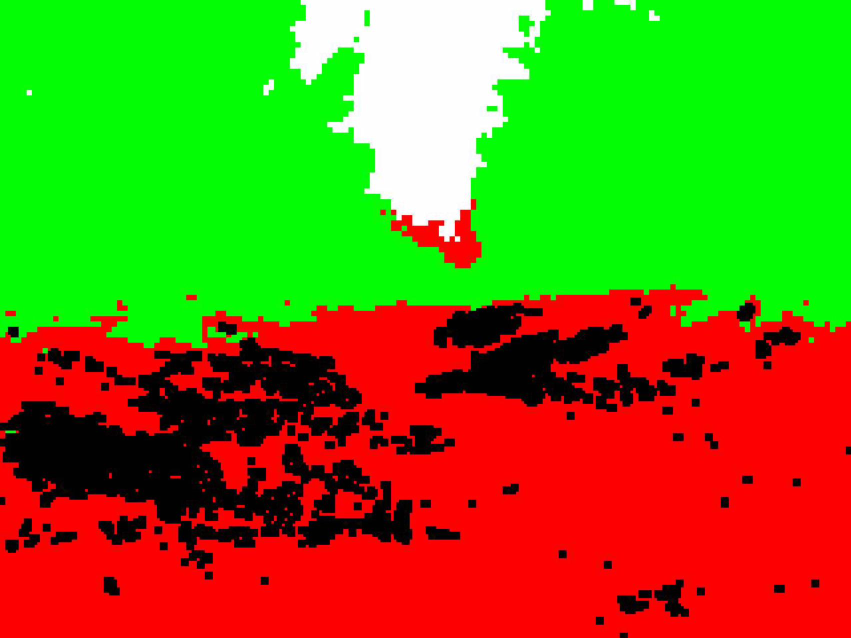
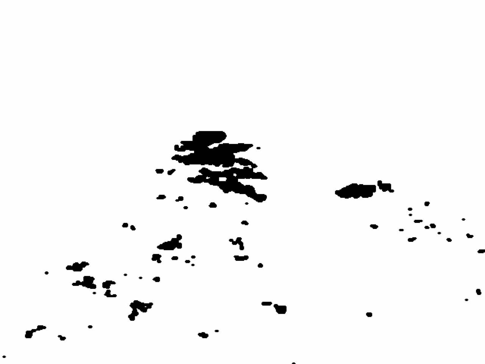
For comparison purposes, we introduce Fig. 8. Right image shows a composition of

the detections provided by our system and Montalvo’s system, where black pixels correspond to those pixels, of the original capture, that were determined as weed or vegetation by our noisy ensemble and the Montalvo’s system. Green pixels

correspond to weeds detected only by our system, and red pixels are those weeds identified only by Montalvo’s system.

It could be interesting to combine the results of both systems with the intersection or union of the weed detection masks. On one hand, the intersection of two good weed identifiers could provide a more sophisticated detection. Spraying could be

minimised and treatment could be only applied on those zones with high probability of containing weeds. On the other hand, the “union” of the two classifiers could also

be interesting, if the treatment depends on the number of detectors that have identified a zone as weeds, e.g, a reduced or different treatment could be applied if only one detector identifies a zone as weeds, and the complete treatment may be

applied when both agree in detecting weeds.

4.4 Future work

As future work, our intention is to introduce more sensors to the current system. One of these new sensors is a second camera with exactly the same features to

18

perform stereo vision. With stereo vision, the position of the weeds with respect to the robot can be directly calculated if the pair of cameras are calibrated.

Moreover, other interesting weed and vegetation detectors, will be considered to

improve the detection of weeds on soil. According to the experiments done with the system provided by Montalvo, their system and our provided similar performance

but they slightly differ on detecting weeds. Although we consider that integrating some different weed detection alternatives can be beneficial to efficiently detect weeds, it is important to mention that computational cost may increase since two,

or more, detectors are applied together.

5 Conclusions

This paper introduces a new system for weed detection into orange groves based on ensembles of neural networks. Due to the features of weed detection, mainly

changes in weather and light conditions, a noisy learning procedure was proposed. This new system provides a final classification image which includes the main

areas of the capture and indicates the presence of weeds on the soil.

Firstly, the new noisy learning was succesfully tested with four ensemble models and nineteen classification problems from the UCI repository of machine learning.

This first comparison was carried out in order to determine the performance of the proposed learning procedure with well-known and publicly available datasets. The

results showed that proposed Noisy learning provides better mean PER values than the traditional training and other noisy ensembles (bagnoise), the increase is around 5% in the majority of cases, and the improvements were statistically

significant. The best classfier with traditional training provided a mean PER of 32.4% whereas the best noisy classifier, generated with CVCv3Conserboost, provided a 37.9%.

The new learning procedure was used in the two-stage weed detector. Our system was tested with 130 testing images taken from seven orange groves and the results

showed that CVCv3Conserboost trained with the proposed noisy learning provided the best mean performance (mean percentage of correctly classified areas in the test set captures) in the first stage, concretely it provided a mean performance of

95.0%. In the second stage, weed detection was also performed with CVCv3Conserboost and the proposed noisy learning since it also provided the best

mean performance (92.28%).

According to the results shown, the new noisy learning is an appropriate alternative for weed detection tasks. Moreover, it is important to mention that the

post-processing procedure applied after the second classification (filtering) ensures that small weed areas would not be considered for treatment thereby reducing the

chemical inputs which is one of the main goals of this research.

Acknowledgments

This paper describes research carried out at the Robotic Intelligence Laboratory. Partial support was provided by Generalitat Valenciana (GV/2010/087), and

Fundació Caixa Castelló - Bancaixa (P1-1A2008-12). We would like to thank to the experts Enrique Fortuño and Patricio Nebot Sr. for granting us access to their

groves and for their valuable advice and help.

19

References

Asif, M., Amir, S., Israr, A., & Faraz, M. (2010). A vision system for autonomous weed detection robot. International Journal of Computer and Electrical Engineering , 2 (3), 486–491.

Asuncion, A., & Newman, D. (2007). UCI machine learning repository. University of California, Irvine, School of Information and Computer Sciences.

Bishop, C. M. (1995). Neural Networks for Pattern Recognition. Oxford University Press, Inc., New York, NY, USA.

Bishop, C. M. (2006). Pattern Recognition and Machine Learning. Springer.

Bossu, J., Gee, C., & Truchetet, F. (2008). Development of a machine vision system for a real time precision sprayer. Electronic Letters on Computer Vision and Image Analysis , 7 (3), 54–66.

Burks, T., Shearer, S., Heath, J., & Donohue, K. (2005). Evaluation of neural-network classifiers for weed species discrimination. Biosystems Engineering , 91 (3), 393–304.

Cho, S. I., Lee, D. S., & Jeong, J. Y. (2002). Automation and emerging technologies: Weed-plant discrimination by machine vision and art ificial neural network. Biosystems Engineering , 83 (3), 275-280.

Cruz-Ramirez, M., Hervás-Martínez, C., Jurado-Expósito, M., & López-Granados, F. (2012). A multi-objective neural network based method for cover crop identification from remote sensed data. Expert Systems with Applications (39), 10038-10048.

Dietterich, T. G. (2000). Ensemble methods in machine learning. In J. (. Kittler (Ed.), First International Workshop on Multiple Classifier Systems. Volume 1857 of Lecture Notes in Computer Science. (pp. 1-15). Springer.

Jang, M., & Cho, S. (1999). Ensemble learning using observational learning theory. International Joint Conference on Neural Networks. 2, pp. 1287–1292. IEEE.

Karimi, Y., Prasher, S. O., McNairn, H., Bonnell, R. B., Dutilleul, P., & Goel, P. K. (2005). Classification accuracy of discriminant analysis, artificial neural networks, and decision trees for weed and nitrogen stress detection in corn. Transactions of the ASAE , 48 (3), 1261–1268.

Kuncheva, L., & Whitaker, C. J. (2002). Using diversity with three variants of boosting: Aggressive, conservative and inverse. Third International Workshop on Multiple Classifier Systems. Volume 2364 of Lecture Notes in Computer Science. Springer.

Montalvo, M., Guerrero, J. M., Romeo, J., Emmi, L., Guijarro, M., & Pajares, G. (2013). Automatic expert system for weeds/crops identification in images from maize fields. Expert Systems with Applications , 40 (1), 75-82.

Moshou, D., Vrindts, E., Ketelaere, B. D., Baerdemaeker, J. D., & Ramon, H. (2001). A neural network based plant classifier. Computers and Electronics in Agriculture , 31 (1), 5-16.

Nebot, P., Torres-Sospedra, J., & Martínez, R. J. (2011). A new HLA-based distributed control architecture for agricultural teams of robots in hybrid applications with real and simulated devices or environments. Sensors , 11 (4), 4385–4400.

Pao, Y. H. (1989). Adaptive Pattern Recognition and Neural Networks. Addison Wesley, New York.

Raviv, Y., & Intratorr, N. (1996). Bootstrapping with noise: An effective regularization technique. Connection Science, Special issue on Combining Estimators (8), 356–372.

Ripley, B. D. (1996). Pattern Recognitionand Neural Networks. Cambridge University Press, Cambridge, UK.

20

Rumelhart, D. E., & McClelland, J. (1986). Parallel Distributed Processing. Explorations in the Microstructure of Cognition. MIT Press.

Rumelhart, D. E., Hinton, G., & Williams, R. (1988). Learning representations by back-propagating errors. Neurocomputing: foundations of research , 696-699.

Stayte, L., & Vaughan, A. (2000). Taking the pith: The impact of the production and consumption of oranges and orange juice on people and environment.

Sung, G.-Y., Kwak, D., & Lyou, J. (2010). Neural network based terrain classification using wavelet features. Journal of Intelligent and Robotic Systems , 59 (3-4), 269–281.

Tellaeche, A., Burgos-Artizzu, X., Pajares, G., & Ribeiro, A. (2007). A vision-based hybrid classifier for weeds detection in precision agriculture through the bayesian and fuzzy k-means paradigms. Advances in Soft Computing. Special Issue: Innovations in Hybrid Intelligent Systems , 44, 72-79.

Tellaeche, A., Pajares, G., Burgos-Artizzu, X., & Ribeiro, A. (2011). A computer vision approach for weeds identification through support vector machines. Applied Soft Computing , 11, 908–915.

Torres-Sospedra, J. (2011). Ensembles of Artificial Neural Networks: Analysis and Development of Design Methods. Ph.D. thesis, Department of Computer Science and Engineering, Universitat Jaume I.

Torres-Sospedra, J., & Nebot, P. (2011). A new approach to visual-based sensory system for navigation into orange groves. Sensors , 11 (4), 4086–4103.

Tumer, K., & Ghosh, J. (1996). Error correlation and error reduction in ensemble classifiers. Connection Science , 8 (3-4), 385-403.

Yildiz, O. T., & Alpaydin, E. (2006). Ordering and finding the best of k>2 supervised learning algorithms. IEEE Transactions on Pattern Analisys and Machine Intelligence , 38 (3), 39

21

List of Figures

Fig. 1 Flow diagram of the two-stage weed detection. First stage corresponds to

the identification of the main parts of the grove, whereas the second stage processes the original capture to detect weeds on those areas previously identified

as Soil. An example of capture and result is included in the diagram along with some intermediate required images and binary masks.

Fig. 2 2D-representation of four artificial patterns and distance to the nearest

neighbor.

Fig. 3 2D-representation of four artificial patterns and the area in which noise

patterns can be located using three different values of factor .

Fig. 4 Description of the procedure used to generate a noisy pattern. Graphical

meaning of randomvector, randomdirection and randomnoise in a simple 2D

example (n=2). For simplification purposes, reordering is not shown and md refers to mdindex(i).

Fig. 5 Example of noisy training sets. The left image shows the original training

set, the initial sequence of patters (Circle is the first element, Triangle is the

second, Star is the third and Square is the fourth), and the area in which noisy patterns can be located (dotted light circle surrounding patterns). The other two subfigures show the possible training set at two different epochs of the

Backpropagation algorithm. The order, given by the numbers, is different in the two examples and does not correspond to the original in any of them.

Fig. 6 Capture with weed zones marked on it and main statistics extracted from

all the weeds zones: width, height, location, area and weed density. Red boxed

areas are the closest ones to the robotic system, yellow boxed areas are in a intermediate distance, and green boxed areas are distant to the robotic system. Borders between close-medium and medium-large areas are marked on the left

border of the capture with L1 and L2 respectively.

Fig. 7 Visual results. a) and b) introduces the visual representation of the

differences between the results provided by traditional Backpropagation and the new noisy learning where black pixels corresponds to detected weeds. The other

colors correponds to the main elements identification. c), e) and g) show the captures with the weed zoned marked on it (coloured boxes). d), f) and h) show the results of the two-stage system on c), e) and g) images.

Fig. 8 Comparison of Montalvo’s system and ours using the capture from Fig. 1.

Left image shows the weed detection provided by Montalvo’s system (only Stages

1&3) on areas previously identified as Soil by our system. Right image shows a composition of combining weed areas detected by both systems weeds detected

by both systems are shown in black. Green and Red stands for the weeds only identified by our system and Montalvo’s system respectively.

Nomenclature

Npatterns Number of patters in training set

UCI Uvinersity of Irvine, Carlifornia Nepochs Number of epochs in Backpropagation

ATRV-2 All Terrain Robot Vehicle ver.2 e Index of epoch in backpropagation

ANN Artificial Neural Network i Original index of pattern

MLP Multilayer Perceptron index(i) Index of pattern after reordering

MF Multilayer Feedforward xi Pattern (feature vector)

T Training set di Distance to closest pattern

V Validation set mdi Maximum distance allowed for noise

TS Test set α Noise factor

MSE Mean Squared Error randomnoise Noise injected to pattern

PER Percentage of Error Reduction nxi Noisy Pattern (feature vector with noise)

M.PER Mean of PER values WVL Wavelet

T.PER Trimmed mean of PER values. M Mean of wavelet values

Perf.

Performance. Classification rate. Percentage of Correctly Classified samples

E Energy of wavelet values

factorc Normalization of Energy values

Table 1 – Training parameters and mean performance of a single network on 19 benchmarking datasets

database patt. input hidden output step mom. iteration mean perf.

aritm 442 277 9 2 0.1 0.05 2500 75.6 ± 0.7

bala 625 4 20 3 0.1 0.05 5000 87.6 ± 0.6

band 277 39 23 2 0.1 0.05 5000 72.4 ± 1.0

bupa 345 6 11 2 0.1 0.05 8500 58.3 ± 0.6

cred 653 2 15 2 0.1 0.05 8500 85.6 ± 0.5

derma 358 34 4 6 0.1 0.05 1000 96.7 ± 0.4

ecoli 336 7 5 8 0.1 0.05 10000 84.4 ± 0.7

flare 1066 10 11 2 0.6 0.05 10000 82.1 ± 0.3

glas 214 19 3 6 0.1 0.05 4000 78.5 ± 0.9

hear 297 13 2 2 0.1 0.05 5000 82.0 ± 0.9

img 2311 19 14 7 0.4 0.05 1500 96.3 ± 0.2

ionos 351 34 8 2 0.1 0.05 5000 87.9 ± 0.7

mok1 432 6 6 2 0.1 0.05 3000 74.3 ± 1.1

mok2 432 6 20 2 0.1 0.05 7000 65.9 ± 0.5

pima 768 8 14 2 0.4 0.05 10000 76.7 ± 0.6

survi 306 3 9 2 0.1 0.2 20000 74.2 ± 0.8

vote 435 16 1 2 0.1 0.05 2500 95.0 ± 0.4

vowel 990 11 15 11 0.2 0.2 4000 83.4 ± 0.6

wdbc 569 30 6 2 0.1 0.05 4000 97.4 ± 0.3

patt: Total number of patterns in the database

input: Number of input features

hidden: Number of hidden nodes in the hidden layer

output: Number of classes

step: Adaptation step of Backpropagation

mom.: Momentum rate of Backpropagation

iteration: Number of iterations performed in Backpropagation

mean perf.: Mean percentage of correctly classified patterns from TS after running the experiments 10 times

Table 2 – General Information about the seven groves

1st Round Captures 2nd Round Captures

Location Features Orientation Month Hour Weather Month Hour Weather

Almassora Mostly clean NW-SE June 5 P.M. Cloudy Oct. 10 A.M. Cloudy

Borriana Leaves in Soil SW-NE July 10 A.M. Sunny Oct. 1 P.M. Cloudy

La Vall d’Uxò Irregular ground N-S July 1 P.M. Sunny Nov. 11 A.M. Sunny

La Vall d’Uxò Fruits in soil NW-SE July 12 P.M. Sunny Dec. 10 A.M. Sun/Cloud

La Vall d’Uxò Dried leaves & Curved

Row s W-E July 3 P.M. Sunny Nov. 2 P.M. Sunny

Vila-real Fruits&Leaves in soil SW-NE June 9 A.M. Cloudy Sept. 12 A.M. Cloudy

Vila-real Mostly Clean SW-NE July 12 P.M. Sun/Cloud Sept. 10 P.M Cloudy

Table 3 – Ensemble comparison with public datasets. General Results according to Mean PER (M.PER) and trimmed Mean PER (T.PER) for ensembles of 3, 9, 20 and 40 networks trained with the traditional learning procedure (Trad.) and the proposed noisy training (Noisy).

3 nets 9 nets 20 nets 40 nets

ensemble learn. M .PER T.PER M .PER T.PER M .PER T.PER M .PER T.PER

Simple Ensemble Trad. 21.8% 21.3% 23.7% 24.9% 23.7% 23.6% 24.6% 24.6%

Simple Ensemble Noisy 28.4% 28.4% 30.5% 30.6% 30.4% 30.3% 30.9% 30.9%

Bagging Trad. 22.9% 23.7% 27.5% 26.7% 28.3% 27.3% 27.7% 28.6%

Bagging Noisy 25% 24.9% 29% 28.5% 29.4% 29.0% 30.3% 30.1%

Bagnoise - 13.3% 14.6% 12.4% 13.6% 13.1% 15.6% 13.7% 16.0%

CVCv3Conserb-ave Trad. 22.4% 22.2% 28.4% 29.3% 30% 30.8% 30.7% 31.3%

CVCv3Conserb-ave Noisy 32.4% 33.1% 37.1% 37.7% 36.8% 37.6% 35.5% 36.5%

CVCv3Conserb-bst Trad. 17.2% 16.4% 27.5% 28.4% 30.2% 31.2% 31.3% 33.4%

CVCv3Conserb-bst Noisy 22.8% 22.8% 30.9% 31.8% 30.6% 33.0% 32.2% 34.1%

CVCv3WCB-ave Trad. 19.8% 22.1% 28% 28.6% 28.5% 29.6% 32.5% 33.5%

CVCv3WCB-ave Noisy 32.3% 32.4% 36.3% 37.0% 37.9% 38.9% 36.2% 37.0%

CVCv3WCB-bst Trad. 15.7% 17.0% 27.3% 27.7% 29.7% 30.1% 30.4% 30.6%

CVCv3WCB-bst Noisy 29.3% 29.0% 35.1% 35.7% 37% 37.6% 37% 37.8%

ensemble Ensemble model used to generate the classif ier

learn. Learning procedure used. “Trad” stands for the traditional Backpropagation w hereas Noisy corresponds to the new noisy learning. Bagnoise is special and uses its ow n noisy learning procedure

Table 4 – Summarize of the statistical results, t-test, for ensembles of 3, 9, 20 and 40 networks.

ensemble Learning procedures compared 3 nets 9 nets 20 nets 40 nets

Simple Ensemble Noisy vs. Traditional ☑ ☑ ☑ ☑

Bagging Noisy vs. Traditional ☐ ☐ ☐ ☑

Bagging Bagnoise * vs. Traditional ☒ ☒ ☒ ☒

CVCv3Conserb-ave Noisy vs. Traditional ☑ ☑ ☑ ☑

CVCv3Conserb-bst Noisy vs. Traditional ☑ ☑ ☐ ☐

CVCv3WCB-ave Noisy vs. Traditional ☑ ☑ ☑ ☑

CVCv3WCB-bst Noisy vs. Traditional ☑ ☑ ☑ ☑

ensemble Ensemble model used to generate the classif iers

☑ Means that noisy learning is statistically better than Backpropagation for the ensemble model

☐ Means that noisy learning and Backpropagation have not statistical differences f or the ensemble

☒ Means that noisy learning is statistically w orse than Backpropagation for the ensemble model

*Bagnoise is considered a noisy learning in this table

Table 5 - Training parameters of the MLP network and ensemble parameters for Terrain classification

Number of patterns: 48000 (24000 for T and 24000 for V)

Number of nodes: 26 (input) – 18 (hidden) – 4 (Output)

Adaptation Step: 0.10

Momentum rate: 0.05

Number of epochs: 2000

Performance: 92.68±0.3 (independent test set)

α-value (noisy learning): 0.8

Table 6 – Results for the First Stage – Terrain Classification

Mean Performance and Mean PER (M.PER) for ensembles of 20 networks from 130 testing images. Results include the standard error of the mean.

Traditional Learning Noisy Learning

ensemble M ean performance M .PER M ean Performance M .PER

Simple Ensemble 93.35±0.15 9.17±2.11 94.05±0.11 18.66±1.46

CVCv3Conserboost 94.16±0.14 20.24±1.96 95.01±0.08 31.79±1.08

CVCv3WCB 94.31±0.08 22.28±1.09 94.66±0.05 27.1±0.72

ensemble Ensemble model used to generate the classif ier

Mean performance

Mean of the performance (as percentage of 8x8 pixels areas correctly classif ied) for the 130 images along w ith the standard error of the mean

M.PER Mean of the Percentage of Error Reduction w ith respect to the traditional single MLP (PER) for the 130 images along w ith the standard error of the eman

Table 7 - Training parameters of the MLP network and ensemble parameters for Weed Detection

Number of patterns: 75110 (37555 for T and 37555 for V)

Number of input nodes: 12 (input) – 9 (hidden) – 2 (output)

Adaptation Step: 0.10

Momentum rate: 0.05

Number of epochs: 1200

Performance: 88.03±0.1 (independent test set)

α-value (noisy learning): 0.75

Table 8 – Results for the Second Stage – Weed Detection after filtering

Mean Performance and Mean PER (M.PER) for ensembles of 5 networks from 130 testing images. Results includes the standard error of the mean.

Traditional Learning Noisy Learning

ensemble M ean performance M .PER M ean Performance M .PER

Simple Ensemble 89.52±0.16 12.46±1.3 89.99±0.11 16.35±0.96

CVCv3Conserboost 91.65±0.13 30.26±1.09 92.28±0.08 35.52±0.63

CVCv3WCB 91.73±0.08 30.94±0.63 92.28±0.05 35.49±0.41

ensemble Ensemble model used to generate the classif ier

Mean performance

Mean of the performance (as percentage of 2x2 pixels areas correctly classif ied) for the 130 images along w ith the standard error of the mean

M.PER Mean of the Percentage of Error Reduction w ith respect to the traditional single MLP (PER) for the 130 images along w ith the standard error of the eman