Smoothed Particle Hydrodynamics - Home - AMDdeveloper.amd.com/wordpress/media/2012/10/Smoothed...20...
31
Smoothed Particle Hydrodynamics Application Example Alan Heirich| November 29, 2010
Transcript of Smoothed Particle Hydrodynamics - Home - AMDdeveloper.amd.com/wordpress/media/2012/10/Smoothed...20...
Smoothed Particle HydrodynamicsApplication Example
Alan Heirich| November 29, 2010

| Smoothed Particle Hydrodynamics | November 20102
FluidsNavier-Stokes equationsSmoothed Particle HydrodynamicsOpenCL simulation
| Smoothed Particle Hydrodynamics | November 20103
Fluids
Liquids, e.g. water
Gasses, e.g. air
Plasmas
| Smoothed Particle Hydrodynamics | November 20104
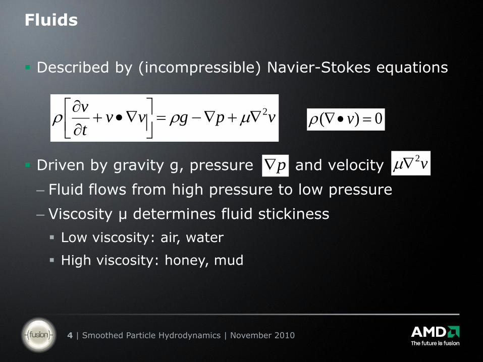
Fluids
Described by (incompressible) Navier-Stokes equations
Driven by gravity g, pressure and velocity
– Fluid flows from high pressure to low pressure
– Viscosity µ determines fluid stickiness
Low viscosity: air, water
High viscosity: honey, mud
vpgvvt
v 2
0)( v
p v2
| Smoothed Particle Hydrodynamics | November 20105
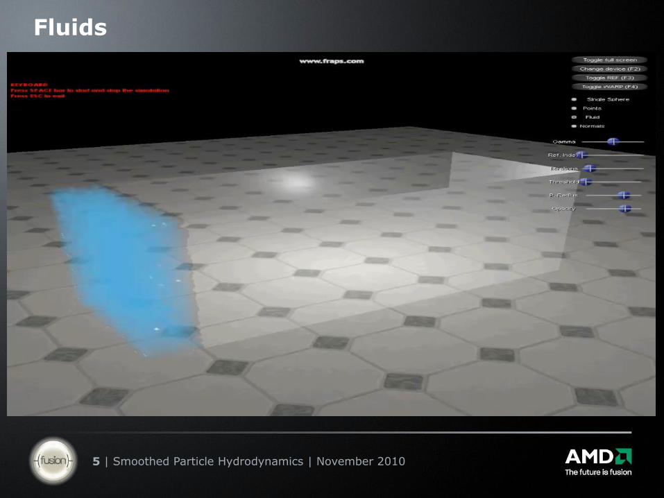
Fluids

| Smoothed Particle Hydrodynamics | November 20106
FluidsNavier-Stokes equationsSmoothed Particle HydrodynamicsOpenCL simulation
| Smoothed Particle Hydrodynamics | November 20107
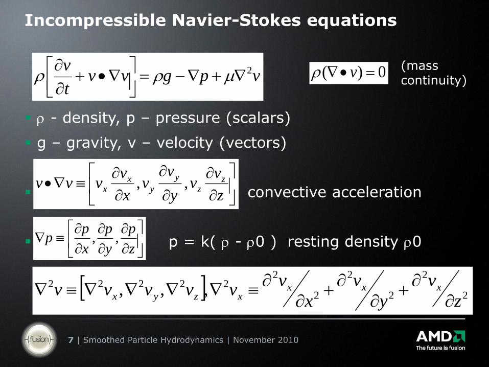
Incompressible Navier-Stokes equations
- density, p – pressure (scalars)
g – gravity, v – velocity (vectors)
convective acceleration
p = k( - 0 ) resting density 0
vpgvvt
v 2
0)( v
z
p
y
p
x
pp ,,
z
vv
y
vv
x
vvvv z
z
y
yx
x ,,
(mass continuity)
2
2
2
2
2
222222 ,,,
z
v
y
v
x
vvvvvv xxx
xzyx
| Smoothed Particle Hydrodynamics | November 20108
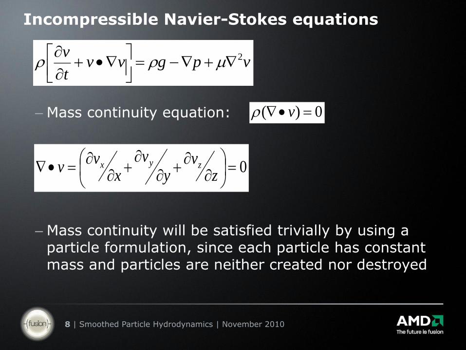
Incompressible Navier-Stokes equations
– Mass continuity equation:
– Mass continuity will be satisfied trivially by using a particle formulation, since each particle has constant mass and particles are neither created nor destroyed
vpgvvt
v 2
0)( v
0
zv
yv
xv
v zyx
| Smoothed Particle Hydrodynamics | November 20109
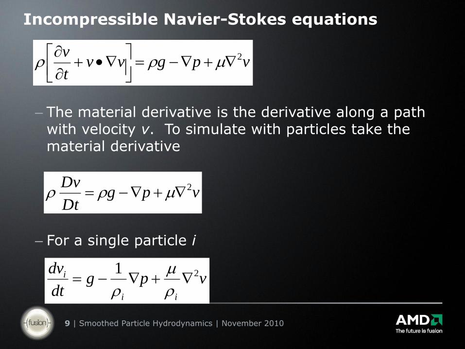
Incompressible Navier-Stokes equations
– The material derivative is the derivative along a path with velocity v. To simulate with particles take the material derivative
– For a single particle i
vpgvvt
v 2
vpgDt
Dv 2
vpgdt
dv
ii
i 21
| Smoothed Particle Hydrodynamics | November 201010
Incompressible Navier-Stokes equations
The Navier-Stokes equations are sensitive to scale, so we simulate them at 0.004x scale relative to the physical environment.
| Smoothed Particle Hydrodynamics | November 201011
FluidsNavier-Stokes equationsSmoothed Particle HydrodynamicsOpenCL simulation
| Smoothed Particle Hydrodynamics | November 201012
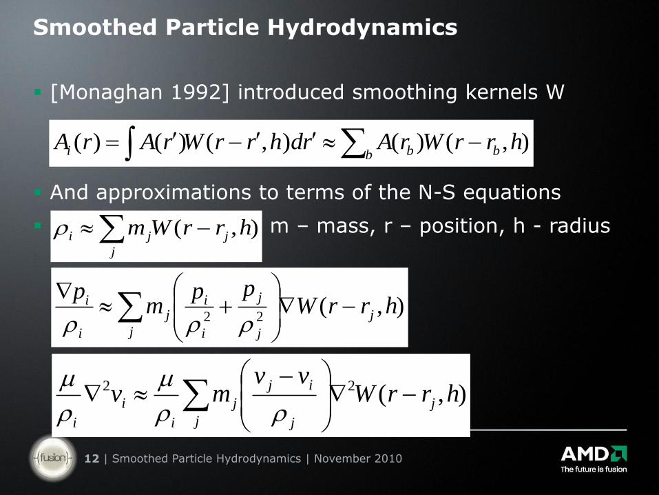
Smoothed Particle Hydrodynamics
[Monaghan 1992] introduced smoothing kernels W
And approximations to terms of the N-S equations
m – mass, r – position, h - radius
),()(),()()( hrrWrArdhrrWrArA bb bi
j
jji hrrWm ),(
),(22
hrrWpp
mp
j
j
j
i
i
j
j
i
i
),(22 hrrWvv
mv j
j
ij
j
j
i
i
i
| Smoothed Particle Hydrodynamics | November 201013
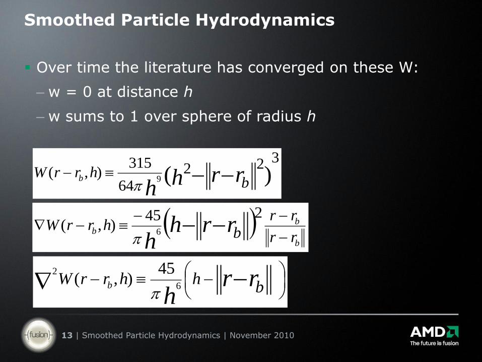
Smoothed Particle Hydrodynamics
Over time the literature has converged on these W:
– w = 0 at distance h
– w sums to 1 over sphere of radius h
)(22
3
64
315),(
9 bhrrW rrh
hb
b
bb
rr
rrb
hrrW rrhh
245),(
6
b
hhrrW rrh
b 6
2 45),(
| Smoothed Particle Hydrodynamics | November 201014
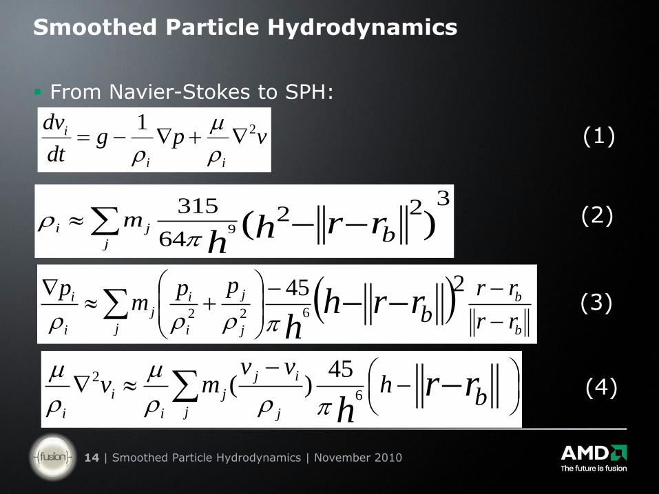
Smoothed Particle Hydrodynamics
From Navier-Stokes to SPH:
vpgdt
dv
ii
i 21
j
ji bm rrh
h)(
223
64
3159
b
b
j
j
i
i
j
j
i
i
rr
rrb
ppm
prrh
h
245622
b
hvv
mv rrhj
ij
j
j
i
i
i
6
2 45)(
(1)
(2)
(3)
(4)
| Smoothed Particle Hydrodynamics | November 201015
FluidsNavier-Stokes equationsSmoothed Particle HydrodynamicsOpenCL simulation
| Smoothed Particle Hydrodynamics | November 201016
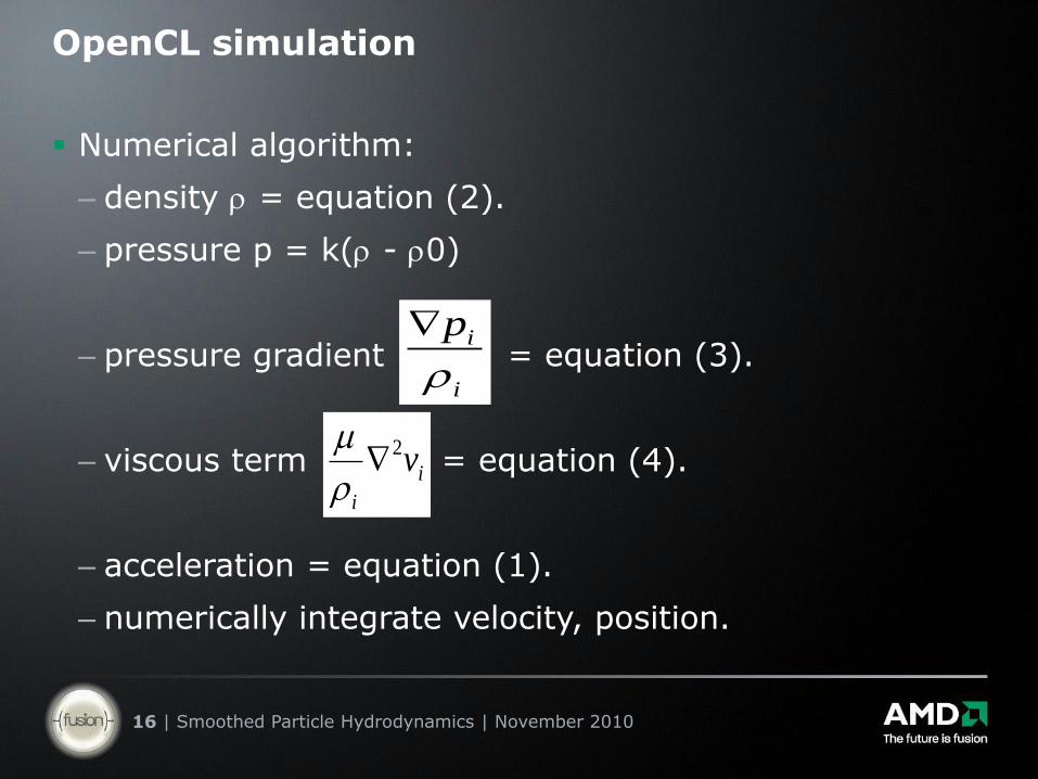
OpenCL simulation
Numerical algorithm:
– density = equation (2).
– pressure p = k( - 0)
– pressure gradient = equation (3).
– viscous term = equation (4).
– acceleration = equation (1).
– numerically integrate velocity, position.
i
ip
i
i
v2
| Smoothed Particle Hydrodynamics | November 201017
OpenCL simulation
A naïve algorithm computes interactions among all particles
– Gives correct result because W= 0 for particles beyond the interaction radius
– But this has complexity O(n^2)
Need an algorithm that only computes interactions among particles that are within the interaction radius
| Smoothed Particle Hydrodynamics | November 201018
OpenCL simulation
A better algorithm partitions space into local regions
– Divide into voxels of size 2h on a side
– Each particle can only interact with particles in the same voxel, and in immediately adjacent voxels
Total search volume = 2x2x2 voxels
– Further refinement: compute interactions with a limited number m of particles
m = 32 works well
| Smoothed Particle Hydrodynamics | November 201019
OpenCL simulation
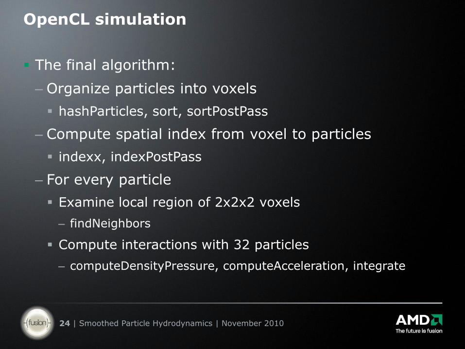
The final algorithm:
– Organize particles into voxels
– Compute spatial index from voxel to particles
– For every particle
Examine local region of 2x2x2 voxels
Compute interactions with 32 particles
| Smoothed Particle Hydrodynamics | November 201020
OpenCL simulation
Interop allows a buffer to be shared between OpenCL and a graphics subsystem.
– This avoids an expensive round trip to host memory
– This is crucial for high performance applications
Due to limits of time we did not implement interop in the graphics code, however we will show you the OpenCL initialization for interop for reference.
| Smoothed Particle Hydrodynamics | November 201021
OpenCL simulation
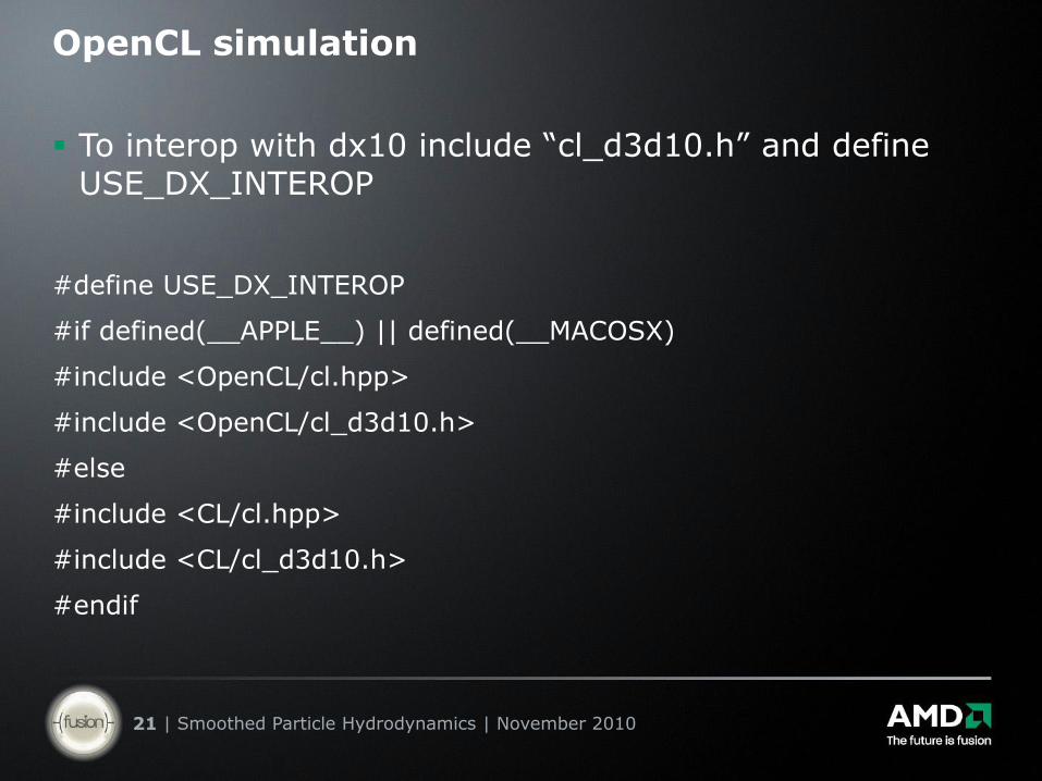
To interop with dx10 include “cl_d3d10.h” and define USE_DX_INTEROP
#define USE_DX_INTEROP
#if defined(__APPLE__) || defined(__MACOSX)
#include <OpenCL/cl.hpp>
#include <OpenCL/cl_d3d10.h>
#else
#include <CL/cl.hpp>
#include <CL/cl_d3d10.h>
#endif
| Smoothed Particle Hydrodynamics | November 201022
OpenCL simulation
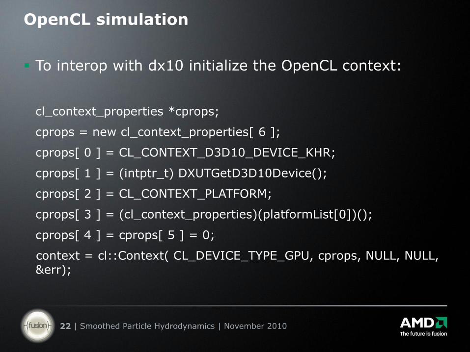
To interop with dx10 initialize the OpenCL context:
cl_context_properties *cprops;
cprops = new cl_context_properties[ 6 ];
cprops[ 0 ] = CL_CONTEXT_D3D10_DEVICE_KHR;
cprops[ 1 ] = (intptr_t) DXUTGetD3D10Device();
cprops[ 2 ] = CL_CONTEXT_PLATFORM;
cprops[ 3 ] = (cl_context_properties)(platformList[0])();
cprops[ 4 ] = cprops[ 5 ] = 0;
context = cl::Context( CL_DEVICE_TYPE_GPU, cprops, NULL, NULL, &err);
| Smoothed Particle Hydrodynamics | November 201023
OpenCL simulation
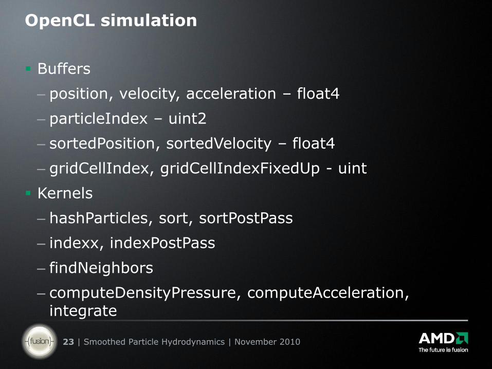
Buffers
– position, velocity, acceleration – float4
– particleIndex – uint2
– sortedPosition, sortedVelocity – float4
– gridCellIndex, gridCellIndexFixedUp - uint
Kernels
– hashParticles, sort, sortPostPass
– indexx, indexPostPass
– findNeighbors
– computeDensityPressure, computeAcceleration, integrate
| Smoothed Particle Hydrodynamics | November 201024
OpenCL simulation
The final algorithm:
– Organize particles into voxels
hashParticles, sort, sortPostPass
– Compute spatial index from voxel to particles
indexx, indexPostPass
– For every particle
Examine local region of 2x2x2 voxels
– findNeighbors
Compute interactions with 32 particles
– computeDensityPressure, computeAcceleration, integrate
| Smoothed Particle Hydrodynamics | November 201025
OpenCL simulation
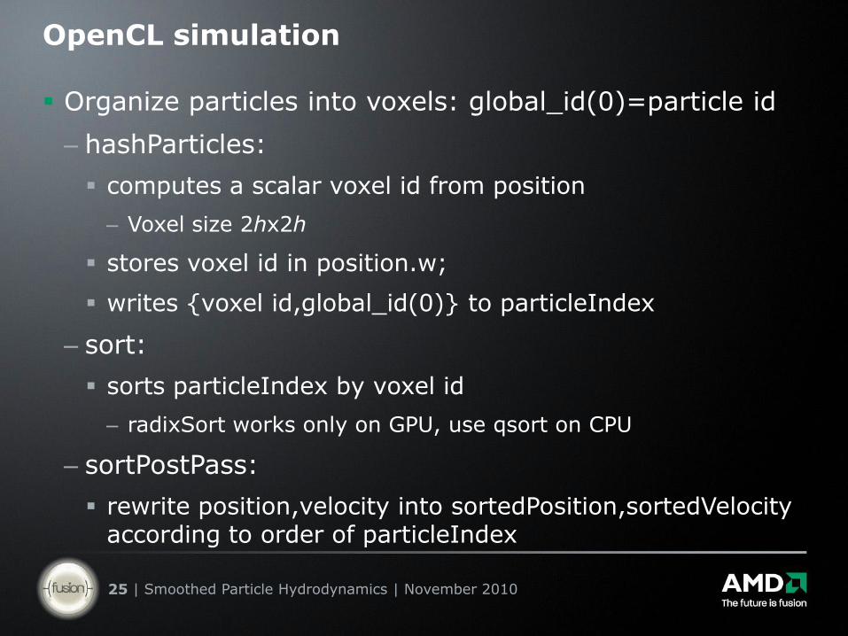
Organize particles into voxels: global_id(0)=particle id
– hashParticles:
computes a scalar voxel id from position
– Voxel size 2hx2h
stores voxel id in position.w;
writes {voxel id,global_id(0)} to particleIndex
– sort:
sorts particleIndex by voxel id
– radixSort works only on GPU, use qsort on CPU
– sortPostPass:
rewrite position,velocity into sortedPosition,sortedVelocityaccording to order of particleIndex
| Smoothed Particle Hydrodynamics | November 201026
OpenCL simulation
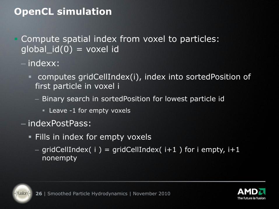
Compute spatial index from voxel to particles: global_id(0) = voxel id
– indexx:
computes gridCellIndex(i), index into sortedPosition of first particle in voxel i
– Binary search in sortedPosition for lowest particle id
Leave -1 for empty voxels
– indexPostPass:
Fills in index for empty voxels
– gridCellIndex( i ) = gridCellIndex( i+1 ) for i empty, i+1 nonempty
| Smoothed Particle Hydrodynamics | November 201027
OpenCL simulation
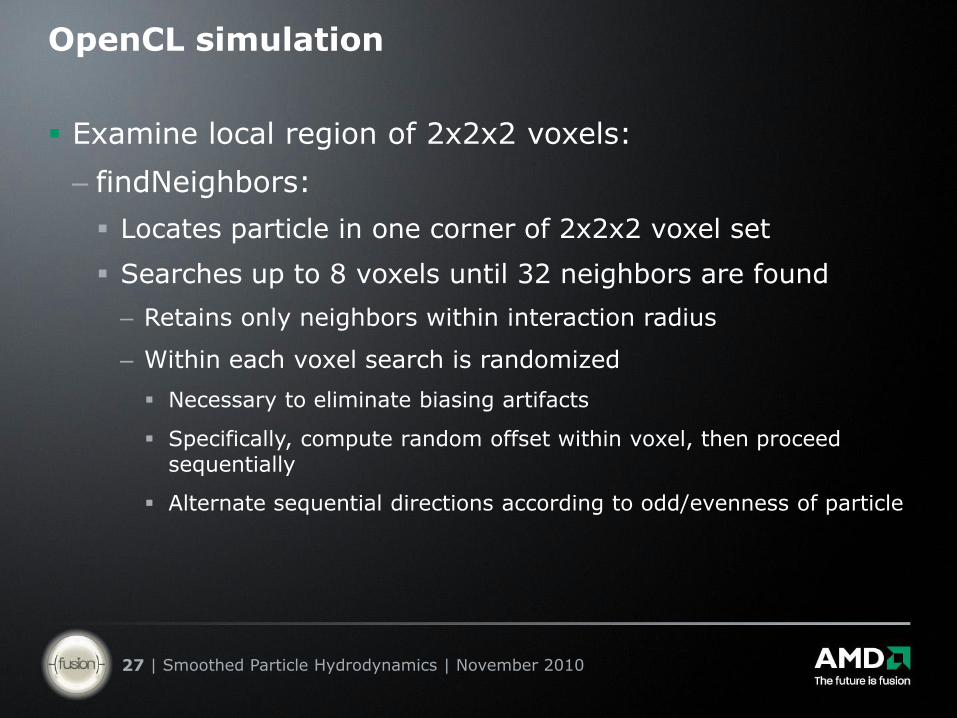
Examine local region of 2x2x2 voxels:
– findNeighbors:
Locates particle in one corner of 2x2x2 voxel set
Searches up to 8 voxels until 32 neighbors are found
– Retains only neighbors within interaction radius
– Within each voxel search is randomized
Necessary to eliminate biasing artifacts
Specifically, compute random offset within voxel, then proceed sequentially
Alternate sequential directions according to odd/evenness of particle
| Smoothed Particle Hydrodynamics | November 201028
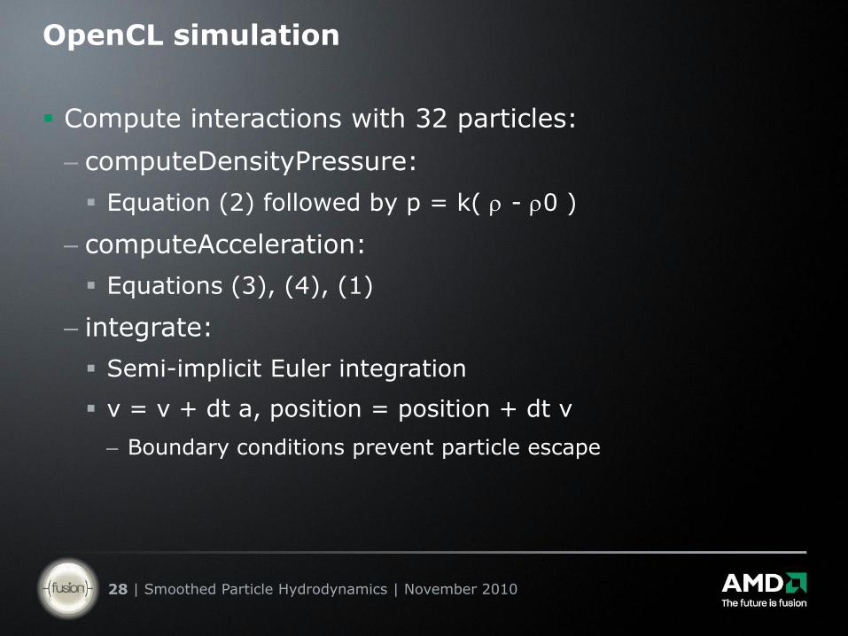
OpenCL simulation
Compute interactions with 32 particles:
– computeDensityPressure:
Equation (2) followed by p = k( - 0 )
– computeAcceleration:
Equations (3), (4), (1)
– integrate:
Semi-implicit Euler integration
v = v + dt a, position = position + dt v
– Boundary conditions prevent particle escape
| Smoothed Particle Hydrodynamics | November 201029
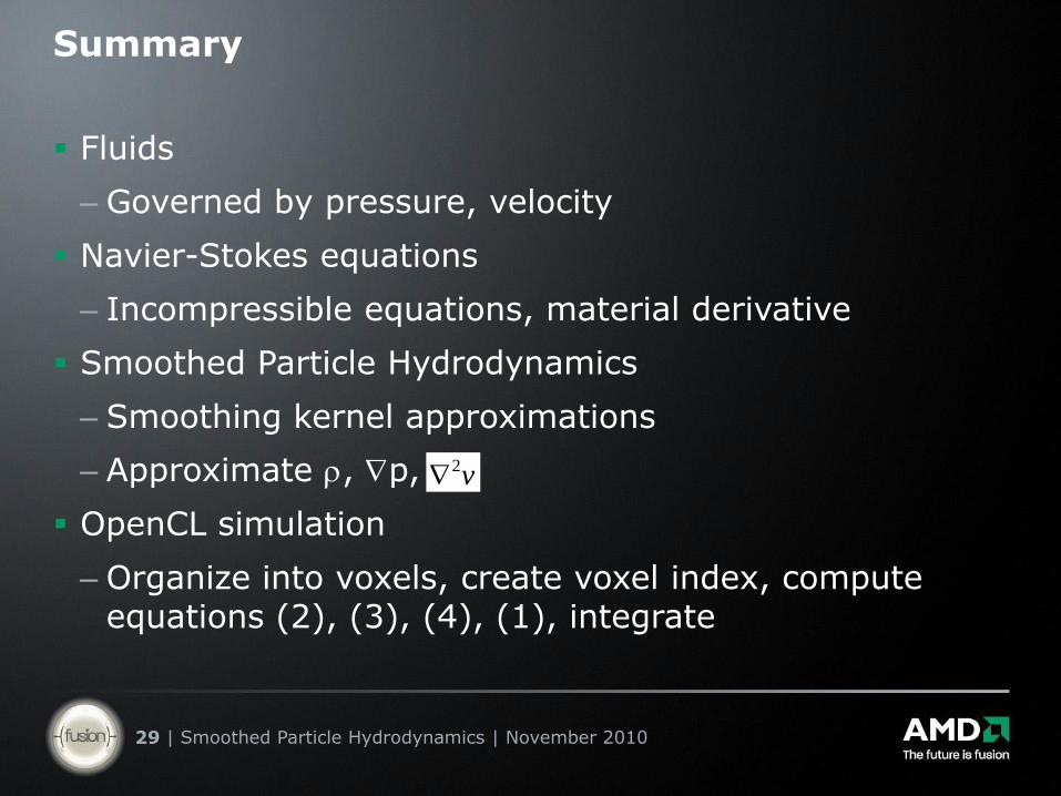
Summary
Fluids
– Governed by pressure, velocity
Navier-Stokes equations
– Incompressible equations, material derivative
Smoothed Particle Hydrodynamics
– Smoothing kernel approximations
– Approximate , p,
OpenCL simulation
– Organize into voxels, create voxel index, compute equations (2), (3), (4), (1), integrate
v2
| Smoothed Particle Hydrodynamics | November 201030
Questions and Answers
Visit the OpenCL Zone on developer.amd.com
http://developer.amd.com/zones/OpenCLZone/
Tutorials, developer guides, and more
OpenCL Programming Webinars page includes:
Schedule of upcoming webinars
On-demand versions of this and past webinars
Slide decks of this and past webinars
Source code for Smoothed Particle Hydrodynamics webinar
| Smoothed Particle Hydrodynamics | November 201031
Trademark Attribution
AMD, the AMD Arrow logo and combinations thereof are trademarks of Advanced Micro Devices, Inc. in the United States and/or other jurisdictions. Other names used in this presentation are for identification purposes only and may be trademarks of their respective owners.
©2009 Advanced Micro Devices, Inc. All rights reserved.