1Bai, H. and B.G. Thomas, “Two Phase Flow in Tundish Nozzles During Continuous Casting ofSteel“, Materials Processing in the Computer Age III, V. Voller and H. Henein, eds., TMSAnnual Meeting, Nashville, TN, March 12-16, 2000, pp. 85-99.

TWO-PHASE FLOW IN TUNDISH NOZZLES

DURING CONTINUOUS CASTING OF STEEL

H. Bai and B. G. Thomas

Department of Mechanical and Industrial EngineeringUniversity of Illinois at Urbana-Champaign1206 West Green Street, Urbana, IL 61801

Ph: 217-333-6919; Fax: 217-244-6534email: h-bai@uiuc.edu; bgthomas@uiuc.edu

Abstract

A three-dimensional finite difference model has been developed to study the liquid steel-argonbubble two-phase turbulent flow in continuous casting tundish nozzles. Experiments have beenperformed on a 0.4-scale water model to verify the computational model by comparing itsprediction with velocity measurements using PIV (Particle Image Velocimetry) technology. Thecomputational model was developed using CFX and then employed to investigate the effects ofvarious casting process variables. A fast, simple inverse model to quantify relationships betweenthose process variables was developed, based on interpolation of the numerical model results,using Bernoulli’s Equation and advanced multivariable curve fitting methods. Predictions usingthis model compare well with plant measurements. The model has been applied to present trendsand observations on the relationship between casting speed, tundish depth, slide gate opening, andargon gas injection rate. The results can also be used to predict the theoretical steel flow ratethrough the nozzle, so that clogging conditions can be identified in the plant.

2Introduction

Tundish nozzle geometry is one of the few variables that are both very influential on the castingprocess and relatively inexpensive to change. Designing an effective nozzle requires quantitativeknowledge of the relationship between nozzle geometry and other process variables on theinfluential characteristics of the flow exiting the nozzle. This relationship depends on the flowpattern within the nozzle components. Most previous modeling studies of flow in the nozzle havefocused on single-phase flow [1-4]. Argon injection into nozzle is an efficient and widelyemployed method to reduce nozzle clogging, even though the real working mechanism(s) are stillnot fully understood [5]. Argon injection may greatly affect the flow pattern in the nozzle, andsubsequently in the mold. Therefore, two-phase flow modeling is needed to improveunderstanding of fluid flow in the nozzle.

In this paper, a three-dimensional finite difference model is developed to study the liquid steel-argon bubble two-phase turbulent flow in the slide-gate tundish nozzles of continuous castingprocess. Experiments have been performed on a 0.4-scale water model at LTV Steel to verify themodel by comparing the model predictions with velocity measurements using Particle ImageVelocimetry. The validated model is then employed to investigate the effects of various castingprocess variables and the complex relationship between them.

Model Formulation

Governing Equations

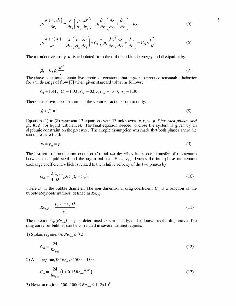
The liquid steel flows from a tundish, through a slide-gate nozzle where it mixes with argonbubbles injected through the nozzle wall, and jets through bifurcated ports into a continuouscasting mold. The flow is inherently three-dimensional, two-phase and highly turbulent. TheReynolds number, based on the nozzle bore diameter (D), is typically of the order of 105. Themultiphase model solves the steady-state mass and momentum conservation equations forincompressible Newtonian fluids where each phase has its own set of continuity and momentumequations. Coupling is achieved through inter-phase drag between liquid steel and argon bubbles.The governing equations for the liquid phase are:

∂∂

( )v f

xl i l

i

[ ] = 0 (1)

ρ∂

∂∂∂

∂∂

µ µ ∂∂

∂∂

ρll j l i l

jl

l

i jl l t

l i

j

l j

il l i

v v f

xf

p

x xf

v

x

v

xf g

( ) ( )( )

( ) ( )[ ] = − + + +

+ + −[ ]c v vl g g i l i, ( ) ( )

(2)and for the gas phase are:

∂∂

( )v f

xg i g

i

[ ] = 0 (3)

ρ∂

∂∂∂

∂∂

µ∂

∂∂

∂ρg

g j g i g

jg

g

i jg g

g i

j

g j

ig g i

v v f

xf

p

x xf

v

x

v

xf g

( ) ( ) ( ) ( )[ ] = − + +

+ + −[ ]c v vl g l i g i, ( ) ( )

(4)where the indices i and j = 1,2,3 represent the x, y and z directions, v u v wi = { , , }, subscript ldonates the liquid phase and subscript g the gas phase, f is volume fraction, ρ is density, µ ismolecular viscosity and µt is the turbulent (or eddy) viscosity. Repeated indices implysummation. Because the density of the gas is 3~4 orders of magnitude smaller than that of theliquid, turbulence in the gas phase is neglected. The standard, two-equation K-ε turbulence modelis chosen for the liquid phase, which requires the solution of two additional transport equations tofind the turbulent kinetic energy, K, and the turbulent dissipation, ε, fields [6],

3ρ

∂∂

∂∂

µσ

∂∂

µ∂∂

∂∂

∂∂

ρ εll j

j j

l

k jl

j

i

i

j

j

il

v K

x x

K

x

v

x

v

x

v

x

( )( )=

+ +

− (5)

ρ∂ ε

∂∂

∂µσ

∂ε∂

ε µ∂∂

∂∂

∂∂

ρ εε

ll j

j j

l

jl

j

i

i

j

j

il

v

x x xC

K

v

x

v

x

v

xC

K

( )( )=

+ +

−1 2

2

(6)

The turbulent viscosity µt is calculated from the turbulent kinetic energy and dissipation by

µ ρεµt lC

K=2

(7)

The above equations contain five empirical constants that appear to produce reasonable behaviorfor a wide range of flow [7] when given standard values as follows:

C1 1 44= . , C2 1 92= . , Cµ = 0 09. , σ K = 1 00. , σε = 1 30.

There is an obvious constraint that the volume fractions sum to unity:

f fl g+ = 1 (8)

Equation (1) to (8) represent 12 equations with 13 unknowns (u, v, w, p, f for each phase, andµt , Κ, ε for liquid turbulence). The final equation needed to close the system is given by analgebraic constraint on the pressure. The simple assumption was made that both phases share thesame pressure field:

p p pl g= = (9)

The last term of momentum equation (2) and (4) describes inter-phase transfer of momentumbetween the liquid steel and the argon bubbles. Here, cl g, denotes the inter-phase momentumexchange coefficient, which is related to the relative velocity of the two phases by

cC

Df v vl g

Dg l l i g i, ( ) ( )= −3

4ρ (10)

where D is the bubble diameter. The non-dimensional drag coefficient CD is a function of thebubble Reynolds number, defined as Rebub

Rebubl l g

l

v v D=

−ρµ

(11)

The function CD (Rebub) may be determined experimentally, and is known as the drag curve. Thedrag curve for bubbles can be correlated in several distinct regions:

1) Stokes regime, 0≤ Rebub ≤ 0.2

CDbub

= 24Re

(12)

2) Allen regime, 0≤ Rebub ≤ 500 ~1000,

CDbub

bub= +( )241 0 15 0 687

ReRe. . (13)

3) Newton regime, 500~1000≤ Rebub ≤ 1~2x105,

4CD = 0 44. (14)

4) Super-critical regime, Rebub > 1~2x105,

CD = 0 1. (15)

Analysis of the results revealed that most bubbles in this study are in the Stokes regime, with afew in the Allen regime. The governing equations (1~8) are discretized using the finite differencemethod and solved with the CFX code version 4.2 developed by AEA Technology [8].

Computational domain and boundary conditions

Figure 1 shows the outline of the computational domain geometry of the slide-gate nozzle, itsboundary condition settings and main dimensions. The top of the nozzle, or the liquid inlet, isspecified as the fixed liquid velocity corresponding to the chosen constant flow rate. Specifically,the average velocity of the liquid at the top was derived from the knowledge of the casting speedand the mold cross-section size. A uniform normal velocity profile was assumed, which is areasonable approximation of the 1/7 power-law turbulent profile expected in pipe flow. Turbulentkinetic energy and turbulent dissipation are also specified at the inlet to the nozzle. They take theaverage values of the profiles calculated from a mixing-length model for turbulent pipe flow [3].The volume fraction of the liquid steel is unity at the top boundary.

Liquid Inletnormal liquid velocity = constantK=constantε =constantf l =1

Gas Iniectionnormal gas velocity = constantf l =1

Outlets (both ports)pressure = constantzero normal gradients for u,v,w,K,ε

z,w

x,uy,v

Main Dimensions and simulation conditions

SEN bore diameter 78 mm Port width x height 78x78 mm x mm Port thickness 30 mm Port angle 15° down Recessed bottom design well depth 12 mm UTN top diameter 114 mm UTN length 241.5 mm Slide-gate thickness 63 mm Slide-gate diameter 78 mm Total length 1152.5 mm Gate orientation 90° SEN submerged depth 200 mm Average bubble diameter 1 mm Molecular viscosity 5.6E-3 kg/m-s of the liquid steel Molecular viscosity 7.4E-5 kg/m-s of the argon gas Density of the 7021 kg/m3

liquid steel Density of the 0.559 kg/m3

argon gas

Figure 1 - Computational domain, boundary conditions, main dimensions and simulationconditions of the standard slide-gate nozzle

The gas injection region, on the surface of the upper tundish nozzle (UTN) wall, is specified as afixed velocity boundary for the gas phase. The fixed normal velocity for the gas phase is the gasinjection flow rate through that region divided by the region area. It should be noted that the argongas flow rate used in modeling is always the “hot” argon flow rate, which is about 5 timesgreater than the “cold” flow rate, as discussed further in the section on simulation conditions.

Fixed pressure boundary conditions are specified at the outlet, or the ports of the nozzle. Thespecified pressure is set to the hydrostatic pressure (which depends on the SEN submergencedepth), which is reasonably close to the actual pressure at the nozzle ports. Zero normal gradients

5are set for all transported variables (u, v, w, Κ, ε ). This treatment of the outlet has proven to be anacceptable approximation for the conditions at the nozzle ports in previous works on single-phaseflow [1-4].

Model Validation

Water model experiments and PIV measurements

Flow visualization and velocity measurements were made using 0.4-scale water models of thetundish, nozzle and mold of the caster at LTV Steel (Cleveland, OH). The nozzle geometry, shownin Table I, was slightly different from the standard conditions used in the parametric study, shownin Figure 1. The PIV (Particle Image Velocimetry) system developed by DANTEC MeasurementTechnology was used to measure the velocity field at the plane of interest near the nozzle port.PIV is a planar measurement technology wherein a pulsed laser light sheet is used to illuminate aflow field seeded with tracer particles small enough to accurately follow the flow. The positions ofthe particles are recorded with a digital CCD (Charged Coupled Device) camera at each instant thelight sheet is pulsed. The images from two neighboring pulses of the light sheet are processed tomatch up individual particles and calculate the vector displacement of each. Knowledge of the timeinterval between the two light sheet pulses then permits the computation of the flow velocity overthe brief time interval, or “exposure”, and the flow velocities thus obtained comprise aninstantaneous velocity field. In this work, the time between pulses in each exposure was 1.5 msand the time between the two neighboring exposures was 0.533 second. To obtain the time-averaged or “steady” velocity field, the results from 50 exposures averaged. Errors in matchingup particles sometimes produce abnormal huge velocities at a single point, which are easy torecognize. Thus, before averaging, the vector plot of each exposure is examined and eachabnormal vector is replaced by the average of its four normal neighbors. If the abnormal vector isat the nozzle port, only the neighbors on the outside of the nozzle port are averaged to obtain thereplacement vector, because velocities inside the nozzle cannot be accurately measured.

Table I Nozzle dimensions and operation conditions for the PIV water experimentsDimension/Condition 0.4 scale Corresponding full scaleBore (SEN) diameter 32 mm 80 mmPort width x height 31mm x 32mm 75mm x 78mmPort thickness 11 mm 27.5 mmPort angle, lower edge 15˚ down 15˚ downPort angle, upper edge 40˚ down 40˚ downRecessed bottom well depth 4.8 mm 12 mmUTN diameter 28 mm 70 mmSlide-gate diameter 28 mm 70 mmSlide-gate thickness 18 mm 45 mmNozzle length - total 510 mm 1275 mmSlide-gate orientation 90° 90°SEN submergence depth 80 mm 200 mmSlide-gate opening (FL) 52% 52%Liquid flow rate at inlet 7.07 x10-4 m3/s 1.042 x10-2 m3/sGas injection volume fraction 5.8% 5.8%Tundish bath depth 400~410 mm 1000~1025 mm

Flow pattern observations

Flow patterns observed in the experiments can be directly compared to the numerical simulationwith the model described above under the same operation conditions. Close agreement betweenthe experiments and the numerical model was achieved. In both the water experiments and modelpredictions, three main recirculation zones are observed in the slide-gate nozzle: in the cavity ofthe middle gate plate, below the throttling gate plate, and at the nozzle ports. High gas

6concentration collects in these recirculation zones. Figure 2 shows an example of the predicted

(A)

E C

E C

(B)

C---C:

(C)

E---E:y

z

Figure 2 - Flow pattern predicted at the SEN ports for the experimental nozzle: (A) end viewfrom the left port, (B) center-plane parallel to the wide face, (C) 12 mm from center-plane, parallel to the wide face

flow pattern near the nozzle ports. In both the simulation and the water experiments, the jet exitsthe ports with a single strong vortex or swirl. The vortex rotational direction is relatively stablewith clockwise direction in a side view (y-z plane) at the plane of the port exit, looking directlyinto the left port (Figure 2A). The jet is directed approximately 29° down, as seen in thephotograph of Figure 3. This is very close to the value of 27.8° down calculated from thesimulation results using a weighted-average method over all nodes on the port plane [9].

Figure 3 - Flow pattern and the average jet angle measurement in water model experiment

No obvious “back-flow” at the nozzle port was observed during the experiments. This matchesthe numerical computation, which predicts only outward flow at the nozzle ports, as shown inFigure 2. It is noted that the observation of no back-flow differs from many previous findings fortypical nozzles [2, 4, 10]. The zero back-flow-zone in the experiments is mainly due to the specialdesign of the SEN ports of this nozzle, which had a much steeper angle of the upper port edges(40°down) than the lower port edges (15°down) [11].

Velocity Comparisons

A quantitative comparison between the PIV measurements and the simulation results is made onthe jet at the nozzle port exit. Unfortunately, the flow field inside the plastic nozzle could not bereliably measured, due to the curvature of the nozzle wall and partial opacity from the machining

7cut. Figure 4(A) shows a vector plot of the PIV-measured flow field around the nozzle port in theplane parallel to the wide face of the mold. The predicted flow vector plots (B) are plotted side byside for direct visual comparison. The magnitudes of the liquid velocity at the port formeasurements and prediction are then extracted and plotted together in (C). Since the PIV is aplanar measurement which does not include v-component of the velocity (y-direction,perpendicular to the paper), the velocity magnitude is calculated using only the u- and w- velocitycomponents. The “overall jet angle”, defined as the weighted-average over the whole 3-D jet [9],should not be compared with the 2-D jet angle calculated from a single slice of the PIVmeasurements, or “slice jet angle”. The slice jet angle is a simple arithmetic average of the jetangles for all measuring points (PIV) or computational cells (CFX) at the slice of the nozzle port.The time-averaged values of the “slice jet angle” are marked on Figure 4 (C).

The upper part of Figure 4 is for the slice through the nozzle center-plane (y=0), and the lowerpart for the slice that is away from and parallel to the center-plane (at y=12mm). The match of thevelocity magnitude and the slice jet angle between the PIV measurement and the model prediction

PredictedMeasured

00.10.20.30.40.50.60

5

10

15

20

25

30

PredictedMeasured

�

00.10.20.30.40.50.60

5

10

15

20

25

30

Liquid velocity (u2+w2)

1/2 (m/s)

Dis

tanc

e fr

om th

e po

rt b

otto

m (

mm

)

z,w

x,u

0.4 m/s

Slice (y=0) at the center-plane of the nozzle, parallel to the wide face of the mold

Slice (y=12mm) away from the center-plane of the nozzle, parallel to the wide face of the mold

(A) PIV measurements (B) CFX prediction (C) Magnitute comparison of PIV measurements and CFX prediction

Slice jet angle:

Predicted: 26.9° upMeasured: 22.8° up

Dis

tanc

e fr

om th

e po

rt b

otto

m (

mm

)

Liquid velocity (u2+w2)

1/2 (m/s)

Slice jet angle:

Predicted: 42.8° downMeasured: 40.3° down

Figure 4 – Comparison of PIV measurements and model prediction

8

y

C

C

E

E

D

D

B

B

A

A

z

00.20.40.60.810

5

10

15

20

25

30 A-A (y=-12mm)B-B (y=-4 mm)C-C (y=0)D-D (y=4 mm)E-E (y=12mm)C-C (y=0),

Liquid velocity (u2+w 2 )1/2 (m/s)

Dis

tanc

e fr

om t

he b

otto

m o

f th

e po

rt (

m)

A-A B-BC-C

E-E

D-D

End view of the nozzle left port

measured

Figure 5 – Velocity profile at different vertical slices of the nozzle port

is satisfactory except that the velocity predictions are consistently slightly larger than themeasurements. This is likely due to fact that the location of the pulsed laser light sheet wasmanually adjusted by naked eye during the PIV experiments, and thus might not lie exactly in thedesired position. Figure 5 shows how the velocity magnitude might change with the slice locationdue to the 3-D effect of the jet vortex. It is interesting to notice the flow vector plot at the sliceaway from the center-plane (lower part of Figure 4). The jet in this slice is upward even thoughthe overall jet is downward. This is consistent with the 3-D swirl of the jet discussed earlier.

Effect of Casting Operation Conditions

The validated two-phase numerical model was next employed to investigate the effects of variousvariables on the flow pattern and important output variables. These variables may include nozzlegeometry and process variables such as casting speed, argon injection flow rate, slide-gateopening and tundish bath depth. The effects of the geometric parameters of the nozzle such as theport angle, port height, port width, port thickness, port sharp and bottom design on flow pattern innozzle as well as on jet characteristics were extensively studied previously with the single-phasefinite element model in previous work [4]. This paper will focus on the effects of the castingprocess variables.

Simulation conditions

The standard nozzle used in this study (shown in Figure 1) has a 90° orientation slide-gate, inwhich the slide-gate moves in a direction perpendicular to the wide face of the mold. Thus, theright and left sides of the mold are symmetrical. This orientation has the least bias flow betweenthe two ports, so is widely adopted in practice. The effect of different orientations of the slide-gatehas been studied elsewhere [9].

Table II - Casting Operation Conditions in Numerical SimulationProcess Variable Symbol Unit Value NotesCasting Speed VC m/min 0.2, 0.5, 1, 1.5, 2.0, 2.3 For 8”x52” slabGate Opening FL % 40, 50, 60, 70, 100 Linear opening

Argon Flow Rate QG SPLM 0, 5, 10 “cold” argon

The casting operation conditions used in this parametric study are listed in Table II. Castingspeed VC refers to a typical size of the continuous casting steel slab (8”x52”) and can be easilyconverted into liquid steel flow rate through the nozzle or casting speed of a different sized-slab.Gate 0pening FL is linear fraction of the opening, defined as the ratio of the displacement of thethrottling plate to the bore diameter of the SEN, and can be converted to any plant definition ofgate opening, usually defined as the relative displacement to a reference position. Calculation [9]shows that argon gas has been heated (when injected through the “hot” nozzle wall) up to 99%of the molten steel temperature even before it hits the liquid steel. The argon flow rate used in thenumerical model should be the “hot” argon flow rate. This is simply the product of the “cold”

9argon flow rate, measured at standard conditions (STP of 25˚C and 1 atmosphere pressure) andthe coefficient of gas volume expansion due to the temperature and pressure change [9], which isabout 5 [12]. For convenience, the equivalent “cold” argon flow rate, which is usually monitoredin the steel plant, will be used in following discussions. All of the 90 (6x5x3) different cases inTable II were simulated with the computational model, in order to perform a full parametric studyon casting speed, gate opening, and argon flow rate.

Inverse model for multiple process variable relationships

For a given nozzle geometry and clogging status, the four basic casting process variables ofcasting speed, argon injection flow rate, gate opening and tundish bath depth are related.Choosing values for any three variables intrinsically determines the fourth. During a stablecasting process, tundish bath depth and argon injection are usually kept at constant level. Gateopening is regulated to compensate for any unwanted effects, such as nozzle clogging andchanges in tundish bath depth, in order to ensure a constant stable casting speed.

In numerical simulation of fluid flow in nozzle, the gate opening is incorporated into thecomputational domain (mesh generation), and casting speed and argon injection flow rate areimplemented as inlet boundary conditions at the top inlet and gas injection region of the nozzle.For each simulation, the numerical model calculates the flow pattern as well as the pressuredistribution, including the pressure-drop across the nozzle, ∆p. The corresponding tundish bathdepth, HT, can be obtained from ∆p by applying a simple relation based on Bernoulli’s Equation,as described next and illustrated in the schematic of the process given in Figure 6.

Tundish

AAAAAAAAAAAAAAAAAAAAAAAAAAAA

AAAAAAAAAAAAAAAAAAAAAAAAAAAAAAAAAAAAAAAAAAAAAAAAAAAAAAAAAAAAAAAA

AAAAAAAAAAAAAAAAAA

AAAA

AAAAAA

AA

AAAAAAAAAAAAA

AAAAAAAAAAAAAAAAAAAAAAAAAAAA

A

B

C

D

HSEN

Mold

Slide-Gate Nozzle

HTz

Figure 6 - Schematic of the continuouscasting process showing tundish, slide-gate nozzle, mold and Location A, B, C,and D

Apply Bernoulli’s Equation on location A and B:

p U gz p U gzA l A l A B l B l B+ + = + +12

2 12

2ρ ρ ρ ρ (16)where p and U are the pressure and velocity atthese locations. Inserting H z zT A B= − , PA = 0and UA ≈ 0 yields

Hp U

gTB l B

l

=+ 1

22ρ

ρ (17)

Apply Bernoulli’s Equation on location C and D:

p U gz p U gzC l C l C D l D l D+ + = + +12

2 12

2ρ ρ ρ ρ (18)

Since H z zSEN D C= − , PD = 0 and UD ≈ 0 , then,

p gH UC l SEN l C= −ρ ρ12

2 (19)

and ∆p p pB C= − (20)

Combining Equation (17), (19) and (20) gives

Hp gH U U

gTl SEN l B C

l

=+ + −∆ ρ ρ

ρ

12

2 2( )(21)

where ∆p is the simulated pressure-drop, HSEN is the SEN submerged depth, UB is the averagevelocity at the top inlet of the nozzle and UC is the average jet velocity at the nozzle port.

10The calculated tundish bath depths (HT) are plotted as a function of the other process variables, inFigures 7(A), (B) and (C). Each point in these plots represents one simulation case. These plotsare inconvenient to apply in practice because tundish bath depth is generally an independentvariable, contrary to the model formulation and results in these three plots. In order to determineand present the results in a more practical manner, an inverse model was developed in order tocapture the results in a flexible manner such that any arbitrary choice of dependent variable ispossible.

The first step in development of this model was to fit the points in Figures 7(A)-(C) using amultiple-variable curve fitting procedure. The lines in Figure 7 are produced with this model,which is briefly described below.

As shown in Figure 7(A), the HT vs. VC data fits well with a second order polynomial function,and data shown in Figure 7(B), (HT vs. QG), fits well with a simple linear function. Unfortunately,a single simple function could not be found to fit the data (HT vs. FL) over the whole FL range.Thus, the HT vs. FL data was split into two regions, with a second order polynomial function forregion FL≤60% and a linear function for region FL≥60%, as shown in Figure 7(C). The overallrelationship can be written as

H a V a V a a F a F a a Q aT C C L L G= + +( ) + +( ) +( )12

2 3 42

5 6 7 8 for FL ≤ 60% (22a)

H a V a V a a F a a Q aT C C L G= + +( ) +( ) +( )92

10 11 12 13 14 15 for FL ≥ 60% (22b)

where the ai (i=1-15) are constants. Expanding this equation yields a new pair of equations with atotal of 18 and 12 unknowns respectively.

H c c V c F c Q c V F c V Q c F Q c V F Q c V c FT C L G C L C G L G C L G C L= + + + + + + + + +1 2 3 4 5 6 7 8 92

102

+ + + + + +c V F c V F c V Q c F Q c V F c V F QC L C L C G L G C L C L G112

122

132

142

152 2

162

+ +c V F Q c V F QC L G C L G172

182 2 for FL ≤ 60% (23a)

H c c V c F c Q c V F c V Q c F Q c V F Q c VT C L G C L C G L G C L G C= + + + + + + + +19 20 21 22 23 24 25 26 272

+ + +c V F c V Q c V F QC L C G C L G282

292

302 for FL ≥ 60% (23b)

where ci (i=1,2,…,30) are all constants. To solve for the 30 constants, 30 equations are needed.Because far more than 30 data sets were simulated (Table II), a least square curve fitting techniquewas used to find ci values that minimize the distance of each data point from its fitting curve [11].The close match in Figures 7(A-C) between the lines from Equation (23) and some of the pointsfrom the computational model indicates the accuracy of this fit.

After constants ci are known, the relatively simple Equation (23) can be inverted into equationsthat have either VC, QG, or FL as the dependent variable (instead of HT). This simple “inversemodel” for multiple process variable relationships can then be used to study how the processvariables are related to each other. The results in Figure 7(D-E) are plotted using this model.

Theoretical steel flow rate

One direct use of the inverse model based on Equation (23) is to predict the theoretical steel flowrate through the nozzle at specific operation conditions (knowing tundish bath depth, gateopening, and argon injection flow rate). Since all simulation cases in Table II are for a non-clogged nozzle, clogging condition can be known by comparing the measured steel flow rate tothe calculated theoretical steel flow rate under the same operation conditions. A clogging indexmay be defined as the ratio of the measured steel flow rate to the predicted theoretical steel flowrate under the same operation conditions.

11

0

0.5

1

1.5

2

0 0.5 1 1.5 2 2.5

Tu

nd

ish

bat

h d

epth

HT (

m)

Casting speed VC

(m/min, for 8"x52" slab)

Argon injection QG=10 SLPM

FL=10%

20%

30%

40%50%

60% 70% 80%

90%

100%

Gate opening FL

0

0.5

1

1.5

2

0 20 40 60 80 100

Tu

nd

ish

bat

h d

epth

HT (

m)

Gate opening FL(%)

Argon injection: 10 SLPM

Casting speed Vc (m/min, for 8"x52" slab)

Vc=2.5

Vc=2.3

Vc=2.0

Vc=1.5

Vc=0.5

Vc=1.0

Vc=0.2

(A) HT vs. VC at different FL and QG =10SLPMCFX data (points) and Eq. 23 (lines)

(B) HT vs. FL at different VC and QG =10SLPMCFX data (points) and Eq. 23 (lines)

0

0.5

1

1.5

2

2.5

3

0 5 10 15

Tu

nd

ish

bat

h d

epth

HT (

m)

Argon injection flow rate: QG(SLPM)

Gate opening FL=50%

casting speed Vc (m/min, for 8"x52" slab)

Vc=2.3

Vc=2.0

Vc=1.5

Vc=1.0

Vc=0.5

Vc=0.20

1

2

3

4

5

0 20 40 60 80 100

HT=1.6m

HT=1.4m

HT=1.2m

HT=1.0m

HT=0.8m

HT=0.6m

HT=0.4m

Cas

tin

g s

pee

d V

C(m/m

in,

8"x5

2" s

lab

)

Gate opening FL (%)

Argon injection: QG=5 SLPM

Tundish bath depth: HT

(C) HT vs. QG at different VC and FL=50%CFX data (points) and Eq. 23 (lines)

(D) VC vs. FL at different HT and QG =5SLPM(Inverse model)

0 0.5 1 1.5 2 2.5 3 3.5 40

20

40

60

80

100

HT=1.6m

HT=1.4m

HT=1.2m

HT=1.0m

HT=0.8m

HT=0.6m

HT=0.4m

Casting speed VC (m/min, 8"x52" slab)

Gat

e o

pen

ing

FL

(%)

Argon injection: Q

G=5 SLPM

Tundish bath depth: HT

0

0.5

1

1.5

2

0 2 4 6 8 10

cast

ing

sp

eed

VC

(m/m

in,

for

8"x5

2" s

lab

)

Argon injection flow rate: QG(SLPM)

Tundish bath depth: HTH

T=1.6m

HT=1.4m

HT=1.2m

HT=1.0m

HT=0.8m

HT=0.6m

HT=0.4m

HT=0.2m Gate opening F

L=50%

(E) FL vs. VC at different HT and QG =5SLPM (F) VC vs. QG at different HT and FL =50%

Figure 7 – Relationship plots of the continuous casting process variables (Tundish bath depth HT,Casting speed VC, Gate opening FL and Argon injection flow rate QG). All lines arefrom relationship model and the points are from the CFX simulation output

12For the example of fixed tundish bath depth (HT), fixed gate opening (FL) less than 60%, andfixed argon injection flow rate (QG), Equation (23) can be rewritten as:

aV bV cC C2 0+ + = (24)

wherea c c F c Q c F c F Q c F QL G L L G L G= + + + + +9 12 13 15

217 18

2 (25a)

b c c F c Q c F c F Q c F QL G L L G L G= + + + + +2 5 6 112

8 162 (25b)

c c c F c Q c F c F Q c F Q HL G L L G L G T= + + + + + −1 3 4 102

7 142 (25c)

The theoretical casting speed is then obtained from:

Vb b ac

aC = − + −2 42

for FL ≤ 60% (26)

The other root is always negative, which is physically incorrect. Similar equations can be derivedfor gate openings greater than 60% and for FL or QG as the dependent variable.

The theoretical steel flow rate is the product of the calculated theoretical casting speed fromEquation (26) and the slab section area (8”x52”). Figure 7(D) shows a graphical representationof the inverse model given by Equation (26).

Relationship between gate opening and steel throughput

Another practical use of the inverse models based on the multiple process variable relationships inEquation (23) is to predict how gate opening changes with casting speed (or steel throughput)under specific tundish bath depth and argon flow rate. In Figure 8, another inverted form ofEquation (23) was applied to make this prediction for conditions where measurements wereavailable for comparison. Specifically, gate openings were recorded for different steel throughputsfor several months at Inland Steel [13], yielding several thousand data points. Only first heats ina sequence were recorded in order to minimize the effect of clogging. The tundish bath depth waskept as a constant (HT=1.125m) for these data, and the argon injection ranged from 7 to 10SLPM. The nozzle geometry used in this plant study is not the same as that of the standardnozzle that Eq. 23 is based on, but it is reasonably close. The main dimensions and operationconditions used for Figure 8 are compared in Table III. The inverse model predictions requiredconversion of FL to the plant definition of gate opening FP and casting speed (m/min) to steelthroughput QFe (metric-tons/min) by

F FP L= − +( %) %1 24 24 (27)and

Q VcFe = 1 8788. (28)

Table III – Dimensions and operation conditions for the standard and Inland nozzlesCondition/Geometry Standard Nozzle Inland NozzleBath depth 1125 mm 1125 mmSEN submerged depth 200 mm 120~220 mmSEN bore 78 mm 91~96 mmGate diameter 78 mm 75 mmGate thickness 63 mm 45 mmPort angle 15° down 35° downPort shape 78mm x 78mm 75mm x 75mmUTN bore 78~114 mm 80~115 mmNozzle total length 1152.5 mm 1123 mmArgon injection 10 SLPM 7~10 SLPM

13In addition to the inverse model, additional CFX simulations were performed for the conditions ofthe Inland nozzle in Table III and the results are shown in Figure 8 as 3 big dots.

Figure 8 shows that these CFX results are very close to the prediction with the inverse model,despite the slight difference in nozzle geometry. In addition to validating both models, thissuggests that the inverse model derived from the standard nozzle is applicable to other practicalconditions, as long as the nozzle geometry is reasonably close.

0.5 1.0 1.5 2.0 2.5 3.0 3.5 4.0 4.50.0

10

20

30

40

50

60

70

80

0

Model prediction(standard nozzle)

CFX simulation (actual nozzle)

Measured data fitting curve

Measured dataA ~ Z

Steel Throughput (metric tons/min)

Slid

e-G

ate

Op

enin

g F

p (

%, p

lan

t d

efin

itio

n)

Measured data legend: A = 1 obs, B = 2 obs, etc. All data for the first heat

AAAAAAAAAAAAAAAAAAAAAAAAAAAAAA

AAAAAAAAAAAAAAAAAAAAAAAA

AAA

Slid

e-G

ate

Op

enin

g F

L (

%)

0

10

20

30

40

50

60

70

Figure 8 – Comparison of the measurement and the model prediction

Both predictions from the inverse model and CFX simulation match the larger extreme of therange of measured gate opening percentage for a given steel throughput. The decreased gateopening often experienced in the plant is likely due to the following reasons:• Rounded edge geometry likely found in the plant nozzles may cause smaller pressure drop

than the sharp edge in new or simulated nozzles [9], thus need less opening to achieve thesame flow.

• Less argon flow in the plant (7~10 SLPM vs. 10 SLPM), needs smaller opening toaccommodate the same liquid flow.

• The initial clogging experienced even during the first heat may reduce the gate openingrequired for a given throughput. This is because, before it starts to restrict the flow channel,the streamlining effect of the initial clogging has been reported to reduce the overall pressureloss [9].

Observations and discussions

The following practical observations can be made from examination of Figure 7:• Higher casting speed can be achieved by a deeper tundish bath depth (constant gate opening)

or larger gate opening (constant bath depth), for a given nozzle geometry and gas flow rate.• To maintain a constant casting speed, a drop of tundish bath depth must be compensated by

increasing the gate opening.• Casting speed is more sensitive to a change in bath depth at low casting speed than at high

casting speed for a given gate opening. This is shown by the flatter slope (dHT/dVC) in thelow casting speed region of Figure 7(A). Thus, a small change in bath depth causes a largerchange in casting speed at low casting speed than it does at high casting speed.

• Casting speed is more sensitive to a bath depth change at large gate opening than at small gateopening (as shown by the steeper slope (dHT/dVC) for smaller gate opening in Figure 7(A)).

• To maintain a constant low casting speed, a larger change in gate opening is needed tocompensate for small changes in bath depth than maintaining a constant high casting speed

14This is as shown by the flatter slope (dHT/dFL) in Figure 7(B) at low casting speed. Castingspeed is more sensitive to gate opening when maintaining a high casting speed.

• For a fixed tundish bath depth, increasing argon injection will slightly slow down the castingspeed (shown in Figure 7(F)) unless the gate opening increases to compensate. This is mainlydue to the extra resistance to steel flow due to the space taken up in the nozzle by the buoyantargon gas.

• To maintain constant casting speed while more argon is injected, either gate opening or bathdepth needs to increase to accommodate the added gas.

• The theoretical casting speed can be calculated from Equation (26) or directly read from theFigure 7(D) for given tundish bath depth, gate opening, and argon injection flow rateQG=5SLPM.

• For a fixed tundish bath depth, casting speed is the most sensitive to gate opening changes atvery large openings (FL>90%) and in the intermediate range of gate opening (FL=40%~60%).This is shown by the steeper slope (dVC/dFL) in Figure 7(D). The intermediate range is mostoften used in practice.

• Figure 7(D, E and F) appears to show that at very low tundish liquid level (HT=0.4m), thecasting speed drops below zero (as reflected in negative or imaginary roots of Equation (26))for small gate opening and large argon flow rate. This is due to the fact that the volumefraction of argon injection becomes abnormally high as the casting speed close to zero, so theflow is very buoyant and the small liquid head in tundish cannot overcome the buoyancy andmaintain a downward flow.

Conclusions

The two-phase turbulent flow of liquid steel and argon bubbles in a slide-gate nozzle can besimulated with a three-dimensional finite difference model. Model predictions agree bothqualitatively and quantitatively with the measurements conducted using PIV (Particle ImageVelocimetry) on a 0.4-scale water model in this paper. Flow through a typical nozzle with 90˚slide-gate orientation has been simulated with the model to investigate the effects of variouscasting process variables and their relationship. A model describing the relationship among thoseprocess variables, based on Bernoulli’s Equation and advanced curve fitting of the multiplevariable numerical results, has been developed and applied to convert the numerical modelingresults to present trends that correspond with real-life operation conditions. With this inversemodel, the theoretical steel flow rate through the nozzle at specific operation conditions can bepredicted and clogging condition can be known by comparing the measured steel flow rate to thepredicted value under the same operation condition.

Acknowledgments

The authors wish to thank the National Science Foundation (Grant #DMI-98-00274) and theContinuous Casting Consortium at UIUC, including Allegheny Ludlum, (Brackenridge, PA),Armco Inc. (Middletown, OH), Columbus Stainless (South Africa), Inland Steel Corp. (EastChicago, IN), LTV Steel (Cleveland, OH), and Stollberg, Inc., (Niagara Falls, NY) for theircontinued support of our research, AEA technology for use of the CFX4.2 package and theNational Center for Supercomputing Applications (NCSA) at the UIUC for computing time.Additional thanks are extended to technicians at LTV Steel for help with the PIV measurements.

Reference

1. D.E. Hershey, "Turbulent Flow of Molten Steel through Submerged Bifurcated Nozzlesin the Continuous Casting Process" (MS Thesis, University of Illinois at Urbana-Champaign, 1992).

2. D. Hershey, B.G. Thomas and F.M. Najjar, "Turbulent Flow through BifurcatedNozzles," International Journal for Numerical Methods in Fluids 17 (1) (1993), 23-47.

3. F.D. Najjar, "Finite-Element Modelling of Turbulent Fluid Flow and Heat TransferThrough Bifurcated Nozzles in Continuous Steel Slab Casters" (MS Thesis, University ofIllinois at Urbana-Champaign, 1990).

4. F.M. Najjar, B.G. Thomas and D. Hershey, "Numerical Study of Steady Turbulent Flowthrough Bifurcated Nozzles in Continuous Casting," Metallurgical Transactions B, 26B(4) (1995), 749-765.

5. K.G. Rackers and B.G. Thomas, "Clogging in continuous casting nozzles" (Paperpresented at SteelMaking Conference Proceedings, 1995), 723-734.

156. B.E. Launder and S.D. B., Mathematical Models of Turbulence, (London: AcademicPress, 1972).

7. B.E. Launder and S.D. B., "Numerical computation of turbulrnt flows," (1974),8. AEA Technology, "CFX4.2 Solver-User's mannual" 19979. B.G. Thomas, "Mathematical Models of Continuous Casting of Steel Slabs" (Annual

Report, Continuous Casting Consortium, University of Illinois at Urbana-Champaign)1998).

10. Y.H. Wang, "3-D mathematical model simulation on the tundish gate and its effect in thecontinuous casting mold" (Paper presented at 10th Process Technology Conference,Toronto, Ontario, Canada, 1992, Iron and Steel Society, Inc.), 75.

11. B.G. Thomas, "Mathematical Models of Continuous Casting of Steel Slabs" (AnnualReport, Continuous Casting Consortium, University of Illinois at Urbana-Champaign,1999).

12. B.G. Thomas, X. Huang and R.C. Sussman, "Simulation of Argon Gas Flow Effects in aContinuous Slab Caster," Metallurgical Transactions B, 25B (4)(1994), 527-547.

13. R. Gass, Private communication, Inland Steel, 1998.