Tutorial on Image Processing in ENVI

1. Opening and Visualizing an image File:

- Click on File -> Open Image File -> Select the GeoTIFF file

‘LISS3_stack_22MAY2012.tif’ -> Click Open. ENVI can open a bunch of different

image types which can be seen in the ‘Open External File’.

- A new window ‘Available Bands List’ opens. To display the image, click on ‘RGB

Color’ in the Available Bands List window -> R: Click on Band 3, G: Click on Band

2, B: Click on Band 1 -> Click Load RGB. This opens the image in 3 windows: #1

(with band compositions and file name), #1 Scroll showing the full image extent and

#1 Zoom. The region within red box of Scroll window is shown in #1 window, and the

region within red box of #1 window is shown in Zoom window, thus creating 3 levels

of data display.

- This is called a False Color Composite. LISS3 sensor onboard ResourceSAT-2

provides data at 24-meter spatial resolution in 4 bands: Green, Red, Near Infrared and

Short Wave IR. To visualize the scene, R is set as NIR band, G is set as Red band and

B is set as Green band.

- To read data of individual pixels, right click on Image -> Cursor Location/Value… A

new window opens up which shows information about the pixel in the crosshairs. This

includes row/column, Latitude and Longitude, Projection, Map co-ordinates and Data

Values.

- To view geo-referencing and other meta data associated with the satellite scene, Right

click on the image name in Available Bands List window-> Click Edit Header.

To further know the Map Information, click on Edit Attributes-> Map Info…

2. Subset a region of interest

To cut out a small portion of the satellite scene, ROI Tool of ENVI is used.

- In the #1 Image window, click on Tools -> Region Of Interest -> ROI Tool.

Subsequently, this can be done by Right clicking on Image -> ROI Tool…

- Within the ROI Tool, select Window: Scroll to subset data by drawing within the Scroll

window.

- Click on ROI_Type -> Rectangle.

- Draw a rectangle within the Scroll window that covers your area of interest and then

right click. The region will now be highlighted in Red. Within the ROI Tool, the

number of pixels, Region # etc are shown.

- Within ROI Tool window, click on File -> Subset Data via ROIs -> Select the desired

Input File.

- Spatial Subset via ROI Parameters window opens. Select the input ROI by clicking on

the Region #1 [Red] -> Specify Output File name and click OK.

- The subset image will be saved in ENVI file format containing a binary image file and

a ‘.hdr’ file containing its header information. The new file will also be added in the

Available Bands List window.

3. Compute Image Statistics

- Click on Basic Tools in main window -> Statistics -> Compute Statistics. (This can

also be done by Right clicking on the image name in Available Bands List window ->

Quick Stats.)

- Select the name of the file you recently subset -> Click OK -> Select Basic Stats,

Histograms. If required, check on Output to a Statistics file / Text Report File.

- Click on Select Plot -> Histogram: Band 1, Histogram: Band 2 etc. to see the

histogram of individual data bands. Other stats like Band wise data min, max, mean

and standard deviation is shown in the Statistics Results window.

4. Visualize Spectra

- Right Click on Image Window -> Z Profile (Spectrum). This shows the Data Value of

a pixel in different bands. Water has maximum reflectance in Green band (i.e. Band 1

of LISS3, typical profile for water pixel shown below).

- Observe the spectrum of other ground objects: bare soil, vegetation etc.

5. Simple Calculations on Images using Band Math

The band values of an image can be used to perform many calculations. Here, we will use

the Band Math Tool of ENVI to extract water pixels within our image. NDWI

(Normalized Difference Water Index) is an index typically used to extract water pixels. It

is given by the formula,

NDWI = (Green-NIR) / (Green + NIR)

Using the LISS3 bands, this index can be easily calculated.

- Click on Basic Tools -> Band Math.

- Enter the expression: (float(b1)-float(b2))/(float(b1) +float(b2))

->

- In the Variables to Band Pairings window, click on B1 -> Click on Band 1(Green) of

LISS3 scene and B2 -> Click on Band 3(NIR) of the scene.

- Specify the output file name (Eg. LISS_NDWI) and click OK.

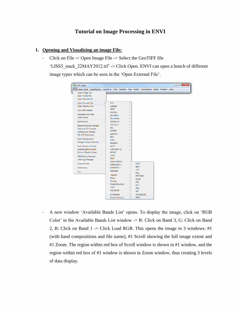
- A new file is added to the Bands List. This file has one band only and a Gray scale

image is displayed by clicking Gray Scale in Available Bands List -> Select Band of

LISS_NDWI -> Load Band.

- Using the Cursor Location/Value option you can see that water pixels have value

greater than 0. All other pixels will have a negative value.

- Again using Band Math, we can create a new image mask which contains water

pixels as 1 and all other pixels as 0. Click on Basic Tools -> Band Math.

- Type in expression: (B1 GT 0). Here GT implies for ‘Greater Than’

- Select B1 and then select the NDWI band computed earlier.

- Enter a name for Output File (Eg. LISS3_water_mask) -> Click OK.

->

- The output image contains a value of 1 where the condition (B1 GT 0) is satisfied.

Hence, the white pixels in the image now represent water. The output image and its

statistics is shown below.