Turbo-AMP: A Graphical-Models Approach to Compressive ...schniter/pdf/lincoln12.pdf · Phil...
28
Phil Schniter The Ohio State University ✬ ✫ ✩ ✪ Turbo-AMP: A Graphical-Models Approach to Compressive Inference Phil Schniter (With support from NSF CCF-1018368 and DARPA/ONR N66001-10-1-4090.) June 27, 2012 1
Transcript of Turbo-AMP: A Graphical-Models Approach to Compressive ...schniter/pdf/lincoln12.pdf · Phil...

Phil Schniter The Ohio State University✬
✫
✩
✪
Turbo-AMP: A Graphical-Models
Approach to Compressive Inference
Phil Schniter
(With support from NSF CCF-1018368 and DARPA/ONR N66001-10-1-4090.)
June 27, 2012
1

Phil Schniter The Ohio State University✬
✫
✩
✪
Outline:
1. Motivation.
(a) the need for non-linear inference schemes,
(b) some problems if interest.
2. The focus of this talk:
(a) compressive sensing (in theory),
(b) compressive sensing (in practice).
3. Recent approaches to these respective problems:
(a) approximate message passing (AMP),
(b) turbo-AMP.
4. Illustrative applications of turbo-AMP:
(a) compressive imaging,
(b) compressive tracking,
(c) communication over sparse channels.
2
Phil Schniter The Ohio State University✬
✫
✩
✪
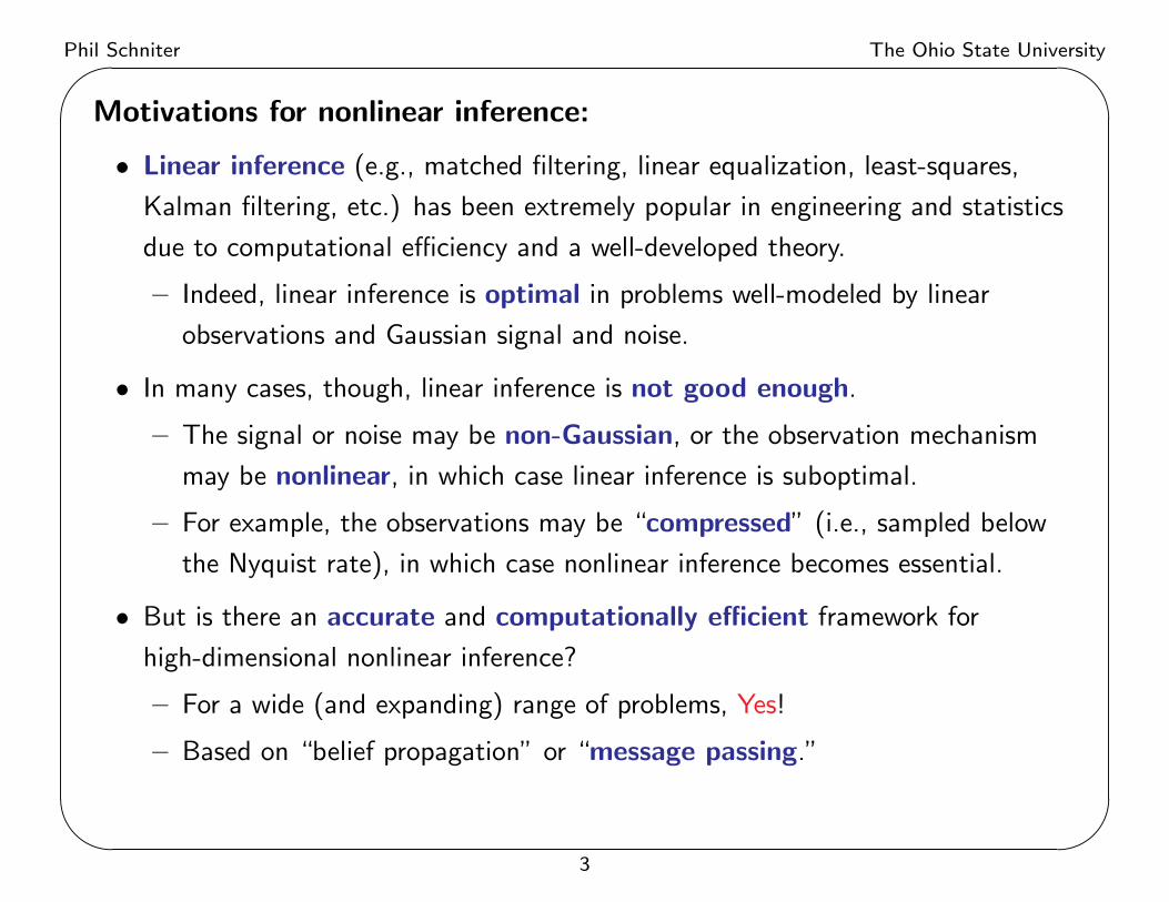
Motivations for nonlinear inference:
• Linear inference (e.g., matched filtering, linear equalization, least-squares,
Kalman filtering, etc.) has been extremely popular in engineering and statistics
due to computational efficiency and a well-developed theory.
– Indeed, linear inference is optimal in problems well-modeled by linear
observations and Gaussian signal and noise.
• In many cases, though, linear inference is not good enough.
– The signal or noise may be non-Gaussian, or the observation mechanism
may be nonlinear, in which case linear inference is suboptimal.
– For example, the observations may be “compressed” (i.e., sampled below
the Nyquist rate), in which case nonlinear inference becomes essential.
• But is there an accurate and computationally efficient framework for
high-dimensional nonlinear inference?
– For a wide (and expanding) range of problems, Yes!
– Based on “belief propagation” or “message passing.”
3

Phil Schniter The Ohio State University✬
✫
✩
✪
A few problems of interest:
Linear additive:
• y =Ax +w with A known, x ∼ px, w ∼ pw
• examples: communications, imaging, radar, compressive sensing (CS).
Generalized linear:
• y ∼ p(y∣z) for z =Ax with A known, x ∼ px
• examples: quantization, phase retrieval, classification.
Generalized bilinear:
• Y ∼ p(Y ∣Z) for Z =AX with A ∼ pA, X ∼ pX
• examples: dictionary learning, matrix completion, robust PCA.
Parametric nonlinear:
• y ∼ p(y∣z) for z =A(θ)x with A(⋅) known, θ ∼ pθ, x ∼ px
• examples: frequency estimation, calibration, autofocus.
4

Phil Schniter The Ohio State University✬
✫
✩
✪
Compressive sensing (in theory):
• Say N -length signal of interest u is sparse or “compressible” in a known
orthonormal basis Ψ (e.g., wavelet, Fourier, or identity basis):
u =Ψx, where x has only K ≪ N large coefficients.
• We observe M ≪ N noisy linear measurements y:
y = Φu +w = ΦΨx +w = Ax +w
from which we want to recover u (or, equivalently, x).
• If A is well-behaved (e.g., satisfies RIP), the sparsity of x can be exploited for
provably accurate reconstruction with computationally efficient algorithms.
– Caution: usually need to tune an algorithmic parameter that balances
sparsity with data fidelity. If using “cross-validation,” this can be expensive!
• Such A results (with high probability) from Φ constructed randomly (e.g., i.i.d
Gaussian) or semi-randomly (e.g., from random rows of fixed unitary Φ).
5

Phil Schniter The Ohio State University✬
✫
✩
✪
Compressive sensing (in practice):
• Usually, real-world applications exhibit additional structure. . .
– in the support of large signal coefficients (e.g., block, tree, etc.),
– among the values of large signal coefficients (e.g., correlation, coherence),
and exploitation of these additional structures may be essential.
• But, exploiting this additional structure complicates tuning, since...
– many more parameters are involved in the model, and
– mismatch in these parameters can severely bias the signal estimate.
• Also, many real-world applications are not content with point estimates. . .
– since the estimates may be later used for decision-making, control, etc.,
– in which case confidence intervals are needed, or preferably the full posterior
probability distribution on the unknowns.
6

Phil Schniter The Ohio State University✬
✫
✩
✪
Solving the theoretical CS problem — AMP:
• Approximate message passing (AMP) [Donoho/Maleki/Montanari 2009/10]
refers to a family of signal reconstruction algorithms that are
– designed to solve the theoretical CS problem,
– inspired by principled approximations of belief propagation.
• AMP highlights:
– Very computationally efficient: a form of iterative thresholding.
– Very high performance (with sufficiently large N,M):
▸ Can be configured to produce near-MAP or near-MMSE estimates.
– Admits rigorous asymptotic analysis [Bayati/Montanari 2010, Rangan 2010]
(under i.i.d-Gaussian A and N,M →∞ with fixed N/M):
▸ AMP follows a (deterministic) state-evolution trajectory.
▸ Agrees with analysis under the (non-rigorous) replica method.
▸ Agrees with belief propagation on sparse matrices, where marginal
posterior distributions are known to be asymptotically optimal.
7

Phil Schniter The Ohio State University✬
✫
✩
✪
Solving practical compressive inference problems — Turbo-AMP:
• The Bayesian graphical-model framework is a flexible and powerful way to
incorporate and exploit probabilistic structure.
x1
x2
x3
x4
x5
y1
y2
y3
AMP
Simple sparsity with known model parameters
p(x∣y)∝M
∏m=1
p(ym∣x)N
∏n=1
p(xn)
8

Phil Schniter The Ohio State University✬
✫
✩
✪
Solving practical compressive inference problems — Turbo-AMP:
• The Bayesian graphical-model framework is a flexible and powerful way to
incorporate and exploit probabilistic structure.
νx
λ
νw
x1
x2
x3
x4
x5
y1
y2
y3
AMP
Simple sparsity with unknown model parameters
Or treat (νw, νx, λ) as deterministic unknowns, and do ≈ML estimation via EM.
9

Phil Schniter The Ohio State University✬
✫
✩
✪
Solving practical compressive inference problems — Turbo-AMP:
• The Bayesian graphical-model framework is a flexible and powerful way to
incorporate and exploit probabilistic structure.
x1
x2
x3
x4
x5
s1
s2
s3
s4
s5
y1
y2
y3
AMP MC
Structured sparsity with known model parameters:
• For these problems, AMP is used as a soft-input soft-output inference block,
like a “channel decoder” in a “turbo” receiver. [Schniter CISS 10]
10

Phil Schniter The Ohio State University✬
✫
✩
✪
Solving practical compressive inference problems — Turbo-AMP:
• The Bayesian graphical-model framework is a flexible and powerful way to
incorporate and exploit probabilistic structure.
νx
λ
νw
ρ
x1
x2
x3
x4
x5
s1
s2
s3
s4
s5
y1
y2
y3
AMP MC
Structured sparsity with unknown model parameters:
• For these problems, AMP is used as a soft-input soft-output inference block,
like a “channel decoder” in a “turbo” receiver. [Schniter CISS 10]
11
Phil Schniter The Ohio State University✬
✫
✩
✪
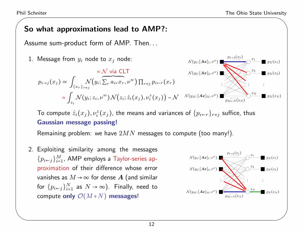
So what approximations lead to AMP?:
Assume sum-product form of AMP. Then. . .
pX(x1)
pX(x2)
pX(xN)
x1
x2
xN
p1→1(x1)
pM←N(xN)
N (y1; [Ax]1, νw)
N (y2; [Ax]2, νw)
N (yM ; [Ax]M , νw)
⋮ ⋮⋮
1. Message from yi node to xj node:
pi→j(xj) ∝ ∫{xr}r≠j
N(yi;≈ N via CLT³¹¹¹¹¹¹¹¹¹¹¹¹¹¹¹·¹¹¹¹¹¹¹¹¹¹¹¹¹¹µ∑r airxr, ν
w)∏r≠j pi←r(xr)
≈∫zi
N(yi; zi, νw)N(zi; zi(xj), νzi (xj)) ∼ N
To compute zi(xj), νzi (xj), the means and variances of {pi←r}r≠j suffice, thus
Gaussian message passing!
Remaining problem: we have 2MN messages to compute (too many!).
2. Exploiting similarity among the messages
{pi←j}Mi=1, AMP employs a Taylor-series ap-
proximation of their difference whose error
vanishes as M→∞ for dense A (and similar
for {pi←j}Ni=1 as N →∞). Finally, need to
compute only O(M+N) messages!
pX(x1)
pX(x2)
pX(xN)
x1
x2
xN
p1→1(x1)
pM←N(xN)
N (y1; [Ax]1, νw)
N (y2; [Ax]2, νw)
N (yM ; [Ax]M , νw)
⋮⋮⋮
12

Phil Schniter The Ohio State University✬
✫
✩
✪
Extrinsic information transfer (EXIT) charts:
EXIT charts, developed to predict the convergence of turbo decoding [ten Brink 01],
can help to understand the interaction between turbo-AMP inference blocks:
0 0.1 0.2 0.3 0.4 0.5 0.6 0.7 0.80
0.1
0.2
0.3
0.4
0.5
0.6
0.7
0.8
MC mutual-info
AMPmutual-info
In this EXIT chart, we are plotting the mutual-information between the true and
(AMP or MC)-estimated support pattern {sn}.
13

Phil Schniter The Ohio State University✬
✫
✩
✪
We will now detail three applications of the turbo-AMP approach:
1. Compressive imaging
. . . with (persistence across scales) structure in the signal support.
2. Compressive tracking
. . . with (slow variation) structure in the signal’s support and coefficients.
3. Communication over sparse channels
. . . involving a generalized linear model, and
. . . where AMP is embedded in a larger factor graph.
14

Phil Schniter The Ohio State University✬
✫
✩
✪
1) Compressive imaging:
• Wavelet representations of natural images are not only sparse, but also exhibit
persistence across scales:
• Can be efficiently modeled using a Bernoulli-Gaussian hidden-Markov-tree:
p(xn ∣ sn) = snN (xn; 0, νj) + (1 − sn)δ(xn) for sn ∈ {0,1}p(sn ∣ sm) ∶ state transition mtx ( p00j 1−p00j
1−p11j p11j) , for n ∈ children(m), j = level(n)
y = Φu +w = ΦΨx +w, w ∼N (0, νw)• The model parameters νw and {νj , p00j , p11j }Jj=0 are treated as random with
non-informative hyperpriors (Gamma and Beta, respectively). We approximate
those messages by passing only the means.
15

Phil Schniter The Ohio State University✬
✫
✩
✪
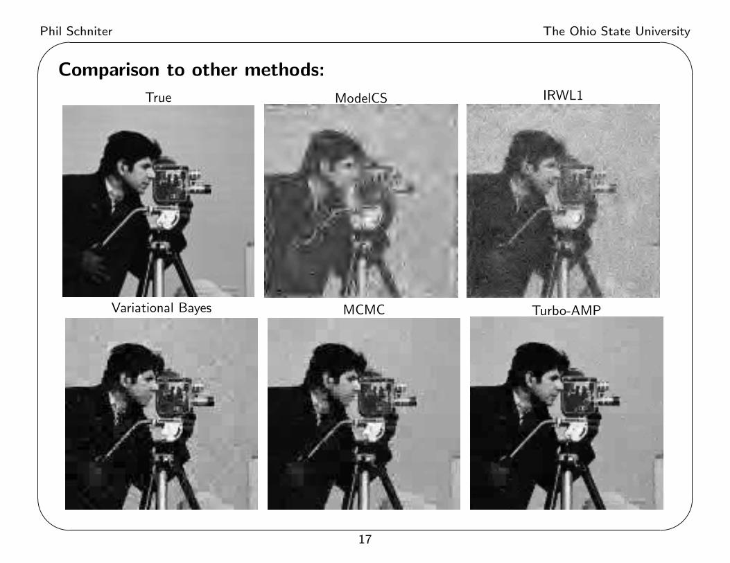
Comparison to other methods:
Average over Microsoft Research class recognition database (591 images):
For M = 5000 random measurements of 128 × 128 images (N = 16384). . .
Algorithm Authors (year) Time NMSE
IRWL1 Duarte, Wakin, Baraniuk (2008) 363 s -14.4 dB
ModelCS Baraniuk, Cevher, Duarte, Hegde (2010) 117 s -17.4 dB
Variational Bayes He, Chen, Carin (2010) 107 s -19.0 dB
MCMC He & Carin (2009) 742 s -20.1 dB
Turbo-AMP Som & Schniter (2010) 51 s -20.7 dB
Turbo-AMP beats other approaches simultaneously in speed and accuracy!
16
Phil Schniter The Ohio State University✬
✫
✩
✪
Comparison to other methods:
True ModelCS IRWL1
Variational Bayes MCMC Turbo-AMP
17

Phil Schniter The Ohio State University✬
✫
✩
✪
2) Compressive tracking / Dynamic compressive sensing:
• Now say we observe the vector sequence
y(t) =A(t)x(t) +w(t), t = 1 ∶ T, w(t)m ∼ i.i.d N (0, νw)with sparse x(t) whose coefficients and support change slowly with time t.
• The slowly varying sparse signal can be modeled as Bernoulli-Gaussian with
Gauss-Markov coefficient evolution and Markov-chain support evolution:
x(t)n = s(t)n θ(t)n for s(t)n ∈ {0,1} and θ(t)n ∈ R
θ(t)n = (1 − α)θ(t−1)n + αv(t)n , v(t)n ∼ i.i.d N (0, νv)p(s(t)n ∣ s(t−1)n ) ∶ state transition matrix ( p00 1−p00
1−p11 p11)
where here the model parameters {νw, νv, α, p00, p11} are treated as
deterministic unknowns and learned using the EM algorithm.
• Note: Our message-passing framework allows a unified treatment of tracking
(i.e., causal estimation of {x(t)}Tt=1) and smoothing.
18

Phil Schniter The Ohio State University✬
✫
✩
✪
Factor graph for compressive tracking/smoothing:
AMP
. . .
. . .
. . .
. . .. . .
⋮ ⋮
⋮ ⋮⋮
⋮⋮
⋮
t
y(1)1
y(1)m
y(1)M
x(1)1
x(1)n
x(1)N
s(1)1
s(1)n
s(1)N
s(2)1
s(2)n
s(2)N
s(T )1
s(T )n
s(T )N
θ(1)1
θ(1)n
θ(1)N
θ(2)1
θ(2)n
θ(2)N
θ(T )1
θ(T )n
θ(T )N
19

Phil Schniter The Ohio State University✬
✫
✩
✪
Near-optimal MSE performance:
−28−27−26−25−24−23−
22
−22
−21
−20
−19
−18
β (E
[K]/M
) (
Mor
e ac
tive
coef
ficie
nts)
→
δ (M/N) (More measurements) →
Support−aware Kalman smoother TNMSE [dB]
0.2 0.4 0.6 0.8
0.1
0.2
0.3
0.4
0.5
0.6
0.7
0.8
0.9
−28−27−26−25−24−23−22
−21
−20
−19
−18
−17
−16
−15
β (E
[K]/M
) (
Mor
e ac
tive
coef
ficie
nts)
→
δ (M/N) (More measurements) →
DCS−AMP TNMSE [dB]
0.2 0.4 0.6 0.8
0.1
0.2
0.3
0.4
0.5
0.6
0.7
0.8
0.9
−25−23−21−19
−19
−17
−17−15
−15−
13−13
−11
−11
−9
−9
−9
−7
−7
−7
−5
−5
−5
−3
−3
−3
β (E
[K]/M
) (
Mor
e ac
tive
coef
ficie
nts)
→
δ (M/N) (More measurements) →
BG−AMP TNMSE [dB]
0.2 0.4 0.6 0.8
0.1
0.2
0.3
0.4
0.5
0.6
0.7
0.8
0.9
• With a Bernoulli-Gaussian signal, the support-aware Kalman smoother
provides an oracle bound on MSE.
• The proposed “dynamic” turbo-AMP performs very close to the bound, and
much better than standard AMP (which does not exploit temporal structure).
20
Phil Schniter The Ohio State University✬
✫
✩
✪
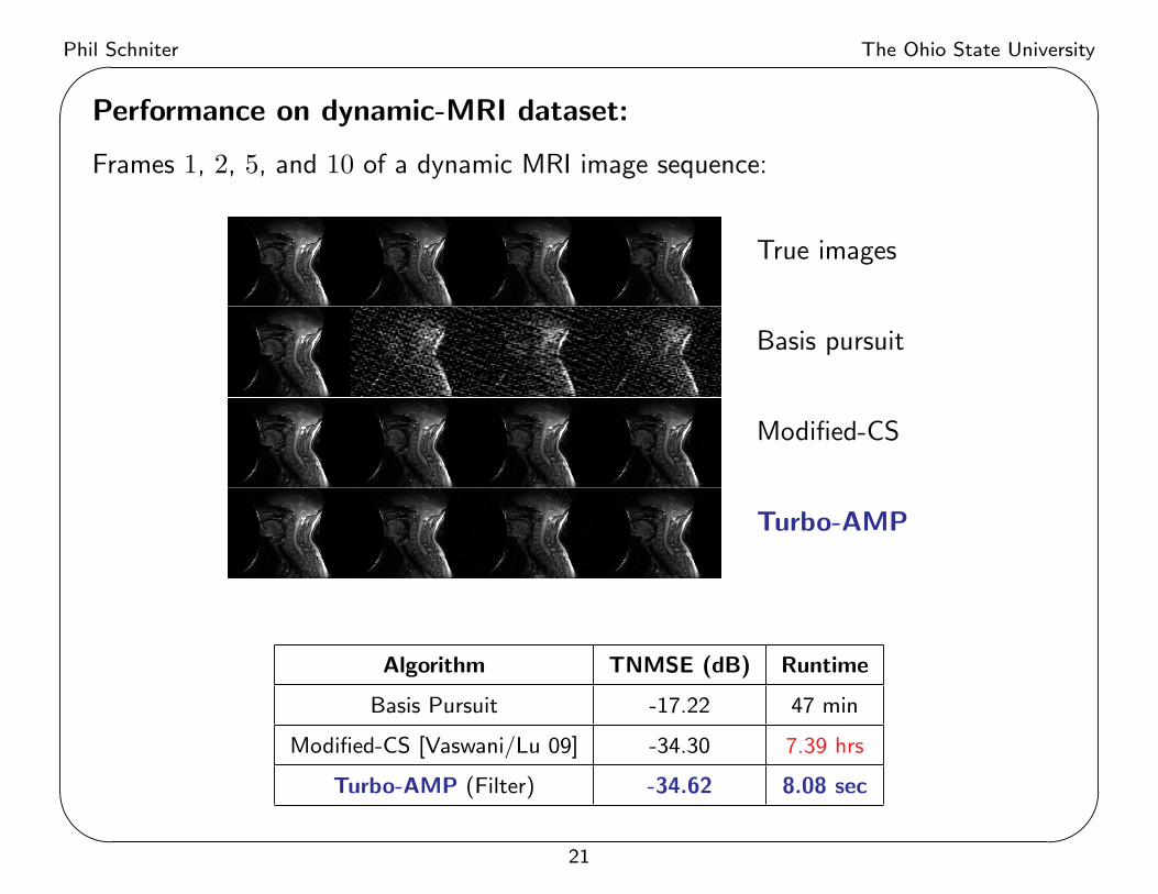
Performance on dynamic-MRI dataset:
Frames 1, 2, 5, and 10 of a dynamic MRI image sequence:
True images
Basis pursuit
Modified-CS
Turbo-AMP
Algorithm TNMSE (dB) Runtime
Basis Pursuit -17.22 47 min
Modified-CS [Vaswani/Lu 09] -34.30 7.39 hrs
Turbo-AMP (Filter) -34.62 8.08 sec
21

Phil Schniter The Ohio State University✬
✫
✩
✪
3) Communication over sparse channels:
• Consider communicating reliably over a channel that is
– Rayleigh block-fading with block length B,
– frequency-selective with delay spread N ,
– sparse impulse response x with K < N non-zero coefs,
where both coefs and support are unknown to the transmitter & receiver.
• The ergodic capacity is C(SNR) = B−KB
log(SNR) +O(1) at high SNR.
• Say, with B-subcarrier OFDM, we use M pilot subcarriers, yielding observations
yp =DpΦpΨx +wp
with known diagonal pilot matrix Dp, selection matrix Φp, and DFT Ψ.
• In “compressed channel sensing” (CCS), the channel x is estimated from yp
and the resulting x is used to decode the (B−M) data subcarriers
yd =DdΦdΨx +wd.
RIP analyses prescribe the use of M = O(K polylogN) pilots, butcommunicating near capacity requires using no more than M =K pilots!
22

Phil Schniter The Ohio State University✬
✫
✩
✪
Rethinking communication over sparse channels:
• The fundamental problem with the conventional CCS approach is the separation
between channel-estimation and data decoding.
• To communicate at rates near capacity, we need joint estimation/decoding,
which we can do using turbo-AMP:
SISO decoding generalized AMP
y0
y1
y2
y3
x1
x2
x3
uniformprior
infobits
code &interlv
pilots &training
codedbits
symbolmapping
QAMsymbs
OFDMobserv
impulseresponse
sparseprior
• Note: Here we need to use the generalized AMP from [Rangan 10]
• Note: We can now place pilots at the bit-level, rather than the symbol level.
23

Phil Schniter The Ohio State University✬
✫
✩
✪
NMSE & BER versus pilot/sparsity ratio (M/K):
• Assume B=1024 subcarriers with K =64-sparse channels of length N =256.
1 2 3 4 5 6−35
−30
−25
−20
−15
−10
−5
0
NM
SE
[dB
]
LMMSELASSOSGBP−1BP−2
BSG
pilot-to-sparsity ratio (M/K)
BP-∞
20dB SNR, 64-QAM, 3 bpcu
1 2 3 4 5 610
−3
10−2
10−1
100
BE
R
LMMSELASSOSGBP−1BP−2
BSG
pilot-to-sparsity ratio (M/K)
BP-∞
20dB SNR, 64-QAM, 3 bpcu
implementable schemes reference schemesLMMSE= LMMSE-based CCS SG= support-aware genieLASSO= LASSO-based CCS BSG= bit- and support-aware genieBP-n=BP after n turbo iterations
• For the plots above, we used M uniformly spaced pilot subcarriers.
• Since spectral efficiency is fixed, more pilots necessitates a weaker code!
24
Phil Schniter The Ohio State University✬
✫
✩
✪
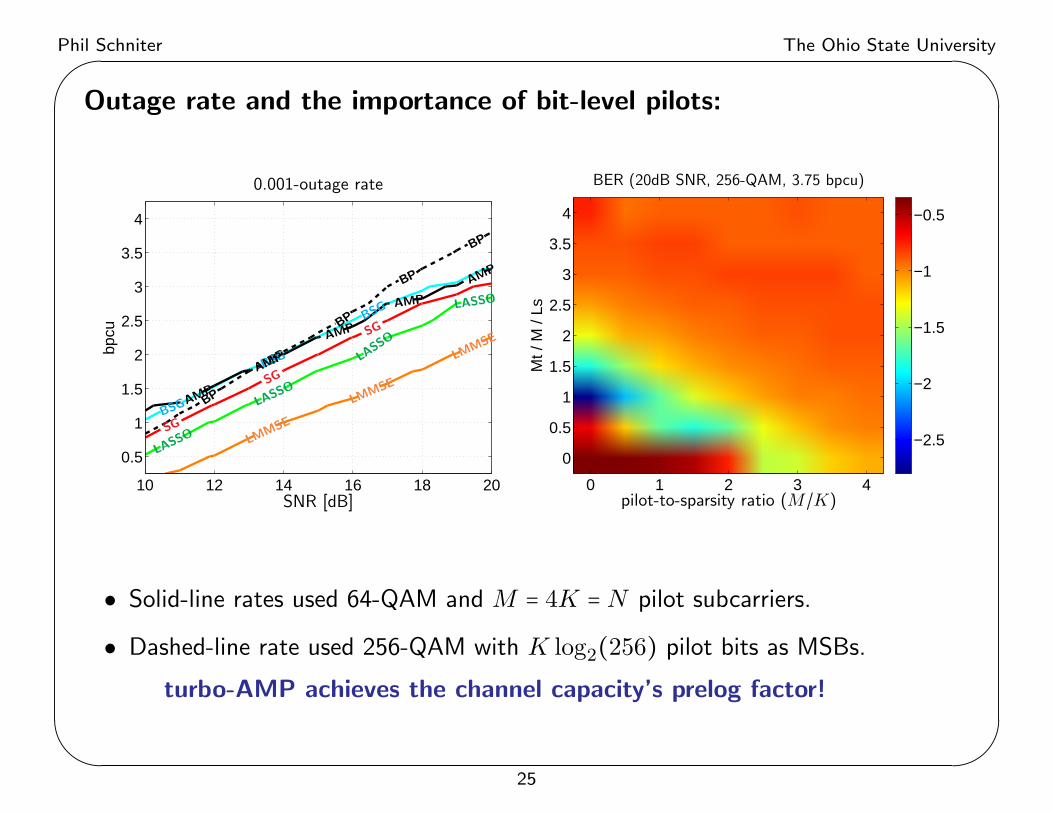
Outage rate and the importance of bit-level pilots:bp
cu
BP
BP
BP
BP
BP
10 12 14 16 18 20
0.5
1
1.5
2
2.5
3
3.5
4
0.001-outage rate
SNR [dB]
BSG
BSG
BSG
AMP
AMP
AMP
AMP
AMP
SG
SG
SG
LASSO
LASS
O
LASS
O
LASS
O
LMMSE
LMMSE
LMMSE
Mt /
M /
Ls
0 1 2 3 4
0
0.5
1
1.5
2
2.5
3
3.5
4
−2.5
−2
−1.5
−1
−0.5
BER (20dB SNR, 256-QAM, 3.75 bpcu)
pilot-to-sparsity ratio (M/K)
• Solid-line rates used 64-QAM and M = 4K = N pilot subcarriers.
• Dashed-line rate used 256-QAM with K log2(256) pilot bits as MSBs.
turbo-AMP achieves the channel capacity’s prelog factor!
25

Phil Schniter The Ohio State University✬
✫
✩
✪
Conclusions:
• The AMP algorithm of Donoho/Maleki/Montanari offers a state-of-the-art
solution to the theoretical compressed sensing problem.
• Using a graphical-models framework, we can handle more complicated
compressive inference tasks, with
– structured signals (e.g., Markov structure in imaging & tracking),
– structured generalized-linear measurements (e.g., code structure in comms),
– self-tuning (e.g., noise variance, sparsity, Markov parameters), and
– soft outputs,
using the turbo-AMP approach, which leverages AMP as a sub-block.
• Ongoing work includes
– applying turbo-AMP approach to challenging new problems, and
– analyzing turbo-AMP convergence/performance.
• Matlab code is available at
http://ece.osu.edu/~schniter/EMturboGAMP
26

Phil Schniter The Ohio State University✬
✫
✩
✪
Thanks!
27

Phil Schniter The Ohio State University✬
✫
✩
✪
Bibliography:
• D. L. Donoho, A. Maleki, and A. Montanari, “Message passing algorithms for compressed sensing,”
Proc. National Academy of Sciences, Nov. 2009.
• D. L. Donoho, A. Maleki, and A. Montanari, “Message passing algorithms for compressed sensing: I.
Motivation and construction,” Information Theory Workshop, Jan. 2010
• M. Bayati and A. Montanari, “The dynamics of message passing on dense graphs, with applications to
compressed sensing,” Trans. IT, Feb. 2011.
• S. Rangan, “Generalized approximate message passing for estimation with random linear mixing,”
arXiv:1010.5141, Oct. 2010.
• P. Schniter, “Turbo reconstruction of structured sparse signals,” CISS (Princeton), Mar. 2010.
• S. Som and P. Schniter, “Compressive imaging using approximate message passing and a Markov-tree
prior,” Trans. SP 2012. (See also Asilomar 2010)
• J. Ziniel and P. Schniter, “Dynamic Compressive Sensing of Time-Varying Signals via Approximate
Message Passing,” arXiv:1205.4080, 2012. (See also Asilomar 2010)
• W. Lu and N. Vaswani, “Modified compressive sensing for real-time dynamic MR imaging,” ICIP, Nov.
2009.
• A. P. Kannu and P. Schniter, “On Communication over Unknown Sparse Frequency-Selective
Block-Fading Channels,” Trans. IT, Oct. 2011.
• P. Schniter, “‘A Message-Passing Receiver for BICM-OFDM over Unknown Clustered-Sparse
Channels,” JSTSP, 2011. (See also Asilomar 2010)
28