TSKS01 Digital Communication Lecture 4 · Digital to analog Analog to digital Medium Digital ......
28
TSKS01 Digital Communication Lecture 4 Digital Modulation – Detection Mikael Olofsson Department of EE (ISY) Div. of Communication Systems
-
Upload
nguyendung -
Category
Documents
-
view
222 -
download
0
Transcript of TSKS01 Digital Communication Lecture 4 · Digital to analog Analog to digital Medium Digital ......
TSKS01 Digital Communication Lecture 4
Digital Modulation – Detection
Mikael Olofsson
Department of EE (ISY)
Div. of Communication Systems

2014-09-23 TSKS01 Digital Communication - Lecture 4 2
A One-way Telecommunication System
Channel
Source encoder
Source decoder
Source
Destination
Channel encoder
Modulator
Channel decoder
De-modulator
Source coding
Channel coding
Packing
Unpacking
Error control
Error correction
Digital to analog
Analog to digital
Medium
Digital modulation

2014-09-23 TSKS01 Digital Communication - Lecture 4 3
Situation
ChannelSender ReceiverSource Destination
Noise
ChannelVector sender
Vector detector
Source DestinationModulatorDe-
modulator
Noise
Vector channelVector sender
Vector detector
Source Destination
Vector noise

2014-09-23 TSKS01 Digital Communication - Lecture 4 4
Last Time – Signals as Vectors
Signals:
Tt <≤0( ) 1,,1,0, −= Mitsi K
ON basis:
( ) ( )
≠=
==∫ ji
jidttt ji
T
ji ,0
,1,
0
δφφ
( ) 1,,1,0, −= Njtj Kφ
Linear combinations:
( ) ( )∑−
=
=1
0,
N
jjjii tsts φ
Vectors:
=
−1,
0,
Ni
i
i
s
s
s M
Inner products (correlation):
( ) ( ) ( ) ,,0
dttbtabaT
∫= ∑−
=
=1
0
N
jjjbaba o
ON basis ⇒ ( ) baba o=,
Norms: ( )aaa ,2 =
aaa o=2
Euclidean distance:
( ) 222 , bababad −=−=
Angles: ( ) ( )ba
ba
ba
ba
⋅=
⋅= ,
cosoα
Equal!
2014-09-23 TSKS01 Digital Communication - Lecture 4 5
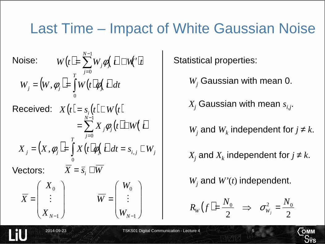
Last Time – Impact of White Gaussian Noise
Received: ( ) ( ) ( )tWtstX i +=
( ) ( ) ( )dtttWWWT
jjj ∫==0
, φφ
Statistical properties:Noise: ( ) ( ) ( )tWtWtWN
jjj ′+=∑
−
=
1
0
φ
( ) ( )tWtXN
jjj ′+=∑
−
=
1
0
φ
( ) ( ) ( )dtttXXXT
jjj ∫==0
, φφ jji Ws += ,
Vectors: WsX i +=
=
−1
0
NX
X
X M
=
−1
0
NW
W
W M
Wj Gaussian with mean 0.
Xj Gaussian with mean si,j.
Wj and Wk independent for j ≠ k.
Xj and Xk independent for j ≠ k.
Wj and W’(t) independent.
( )22
020 NNfR
jWW =⇒= σ

2014-09-23 TSKS01 Digital Communication - Lecture 4 6
AWGN – Additive White Gaussian Noise
Orthogonal noise components are statistically independent.
X1 & X2 independent
Y1 & Y2 independent
PSD = Variance
Y2
Y1
X1
X2
σXi= σYi
= RW ( f ) = N0/22 2

2014-09-23 TSKS01 Digital Communication - Lecture 4 7
Demodulation
ChannelModulatorDe-
modulator
Noise
Projections:
Do this!
Signals are projected on
basis functionsNoise is
projected on basis functions

2014-09-23 TSKS01 Digital Communication - Lecture 4 8
Correlation Receiver

2014-09-23 TSKS01 Digital Communication - Lecture 4 9
Matched Filters
A filter with impulse response hj(t) = φj(T – t) is matched to φj(t).
Example: Usage (φj�hj)(t):
T 2T
Maximum at t = T.
Orthogonal signal φi(t):
Zero at t = T.
T 2T
T
φj(t)hj(t)
Then (φi�hj)(t):
(φi(t),φj(t)) = 0

2014-09-23 TSKS01 Digital Communication - Lecture 4 10
Demodulation Using Matched Filters
ChannelModulatorDe-
modulator
Noise
Do this!
Filter: Matched to
Output:
Sample at t = T : And this!

2014-09-23 TSKS01 Digital Communication - Lecture 4 11
Matched Filter Receiver
2014-09-23 TSKS01 Digital Communication - Lecture 4 12
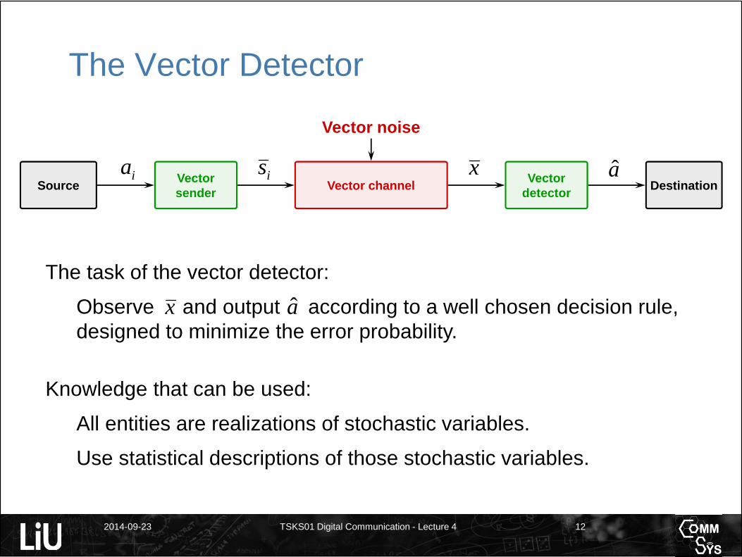
The Vector Detector
Knowledge that can be used:
All entities are realizations of stochastic variables.
Use statistical descriptions of those stochastic variables.
The task of the vector detector:
Observe and output according to a well chosen decision rule, designed to minimize the error probability.
x a
Vector channelVector sender
Vector detector
Source Destination
Vector noise
x aisia

2014-09-23 TSKS01 Digital Communication - Lecture 4 13
1 3
3
1
–1
φ0
φ1
0s
1s
2s
Vector Detection
?
Received vector: x
x
Goal: Minimize the error probability
{ }xXAA =≠ |ˆPr
Estimated symbol
Sent symbol
Received vector
Observed realization
Equivalent decision rule:
Set if is maximized for k = i.
{ }xXaA k == |Priaa =ˆ

2014-09-23 TSKS01 Digital Communication - Lecture 4 14
Independent of ak.
−4−2
02
46
−20
24
680
0.01
0.02
0.03
Detection
Bayes rule: { } ( )( ) { }k
X
kAXk aA
xf
axfxXaA ==== Pr
||Pr |
New decision rule:
Set if
is maximized for k = i.
iaa =ˆ
( ) { }kkAX aAaxf =⋅Pr||
2014-09-23 TSKS01 Digital Communication - Lecture 4 15
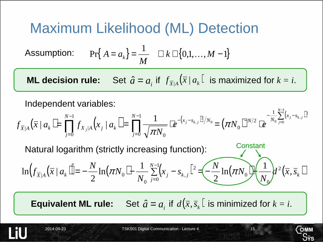
Maximum Likelihood (ML) Detection
Assumption: { } { }1,,1,01
Pr −∈∀== MkM
aA k K
ML decision rule: Set if is maximized for k = i. iaa =ˆ ( )kAX axf ||
( ) ( )∏−
=
=1
0|| ||
N
jkjAXkAX axfaxf
j
Independent variables:
( ) 02
,
1
0 0
1 NsxN
j
jkjeN
−−−
=∏ ⋅=
π( )
( )∑⋅=
−
=
−−−
1
0
2,
0
1
20
N
jjkj sx
NN eNπ
Natural logarithm (strictly increasing function):
( )( ) ( ) ( )∑ −−−=−
=
1
0
2,
00|
1ln
2|ln
N
jjkjkAX sx
NN
Naxf π ( ) ( )ksxd
NN
N,
1ln
22
00 −−= π
Constant
Equivalent ML rule: Set if is minimized for k = i. iaa =ˆ ( )ksxd ,

2014-09-23 TSKS01 Digital Communication - Lecture 4 16
1 3
3
1
–1
φ0
φ1
2s
0s
1s
ML Decision Regions
?
B2
B1
B0
x
Interprete as the nearest signal.x
!
Result:Decision regions consisting of all points closest to a signal point.
Notation:Bi is the decision region of the signal vector si. Thus also of the signal si (t)and of the message ai.
The borders are orthogonal to straight lines between signals:
In 2 dimensions: Lines.In 3 dimensions: Planes.In more dim: Hyperplanes.
Borders cut the lines mid-way.

2014-09-23 TSKS01 Digital Communication - Lecture 4 17
Error Probability
Symbol error probability:
{ } { } { }∑−
=
=≠⋅==≠=1
0e |ˆPrPrˆPr
M
iiii aAaAaAAAP
{ } { }∑−
=
=∉⋅==1
0
|PrPrM
iiii aABXaA
ML detection again { } { }
−∈∀== 1,,1,01
Pr MiM
aA i K :
{ }∑−
=
=∉=1
0e |Pr
1 M
iii aABX
MP ( ) N
M
iiAX dxdxaxf
MLL 1
1
0| |
1∑∫ ∫
−
=
=iBx∉
This is generally hard to calculate.
2014-09-23 TSKS01 Digital Communication - Lecture 4 18
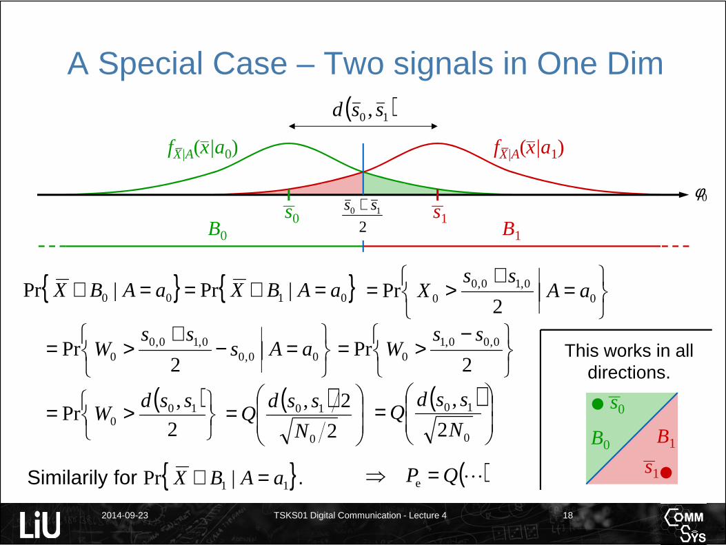
A Special Case – Two signals in One Dim( )10,ssd
B1B0
fX|A(x|a0) fX|A(x|a1)
{ } { }0100 |Pr|Pr aABXaABX =∈==∉
s0 s1
φ0
=
+>= 0
0,10,00 |
2Pr aA
ssX
=−+
>= 00,00,10,0
0 |2
Pr aAsss
W
−
>=2
Pr 0,00,10
ssW
( )
>=
2
,Pr 10
0
ssdW
( )
=
2
2,
0
10
N
ssdQ
( )
=
0
10
2
,
N
ssdQ
Similarily for .{ }11 |Pr aABX =∉
This works in all directions.
B1B0
s0
s1( )LQP =⇒ e
210 ss +

2014-09-23 TSKS01 Digital Communication - Lecture 4 19
Back to M Signals in N Dimensions
1 3
3
1
–1
φ0
φ1
2s
0s
1s
B2
B1
B0
Interprete as the nearest signal.x
We had:
{ }∑−
=
=∉=1
0e |Pr
1 M
iii aABX
MP
{ }∑∑−
= ≠
=∈=1
0
|Pr1 M
i ijij aABX
M
Hard to calculate!!
Could we take this to the more simple case
in one dimension?
2014-09-23 TSKS01 Digital Communication - Lecture 4 20
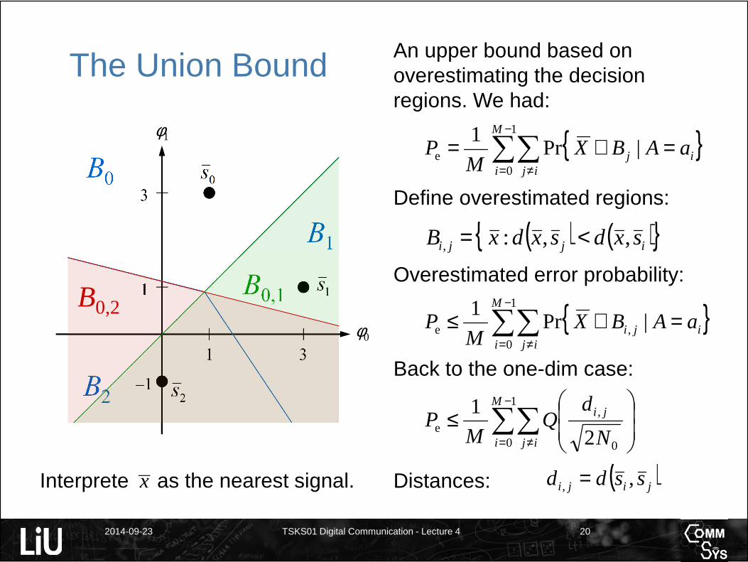
The Union Bound
1 3
3
1
–1
φ0
φ1
2s
0s
1s
B2
B1
B0
Interprete as the nearest signal.x
Define overestimated regions:
( ) ( ){ }ijji sxdsxdxB ,,:, <=
B0,1B0,2
An upper bound based on overestimating the decision regions. We had:
{ }∑∑−
= ≠
=∈=1
0e |Pr
1 M
i ijij aABX
MP
{ }∑∑−
= ≠
=∈≤1
0,e |Pr
1 M
i ijiji aABX
MP
Overestimated error probability:
∑∑−
= ≠
≤
1
0 0
,e
2
1 M
i ij
ji
N
dQ
MP
Back to the one-dim case:
( )jiji ssdd ,, =Distances:
2014-09-23 TSKS01 Digital Communication - Lecture 4 21
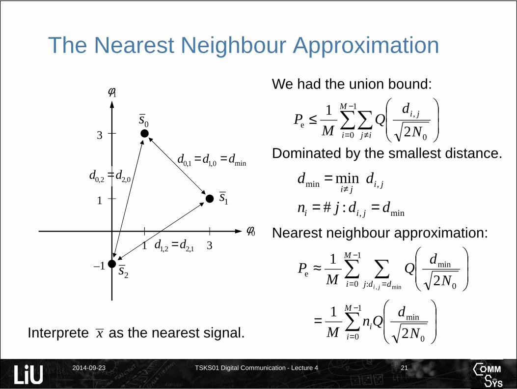
The Nearest Neighbour Approximation
1 3
3
1
–1
φ0
φ1
2s
0s
1s
Interprete as the nearest signal.x
∑∑−
= ≠
≤
1
0 0
,e
2
1 M
i ij
ji
N
dQ
MP
We had the union bound:
0,11,0 dd =
1,22,1 dd =
0,22,0 dd =
∑ ∑−
= =
≈
1
0 : 0
mine
min,2
1 M
i ddj jiN
dQ
MP
Nearest neighbour approximation:
Dominated by the smallest distance.
jiji
dd ,min min≠
=
min,:# ddjn jii ==
∑−
=
=
1
0 0
min
2
1 M
ii
N
dQn
M
mind=

2014-09-23 TSKS01 Digital Communication - Lecture 4 22
Comments
Alternative upper bound:As the union bound, but only consider pairs of points whose decision regions share a common border.
At high SNR Eavg/N0:Both the union bound on – and the nearest neighbour of –the error probability are close to the real error probability.
Alternative approximation:As the nearest neighbour approximation, but consider the two or three smallest distances.
Very simple approximation:
≈
0
mine
2N
dQP
Very simple upper bound:
( )
⋅−≤
0
mine
21
N
dQMP
2014-09-23 TSKS01 Digital Communication - Lecture 4 23
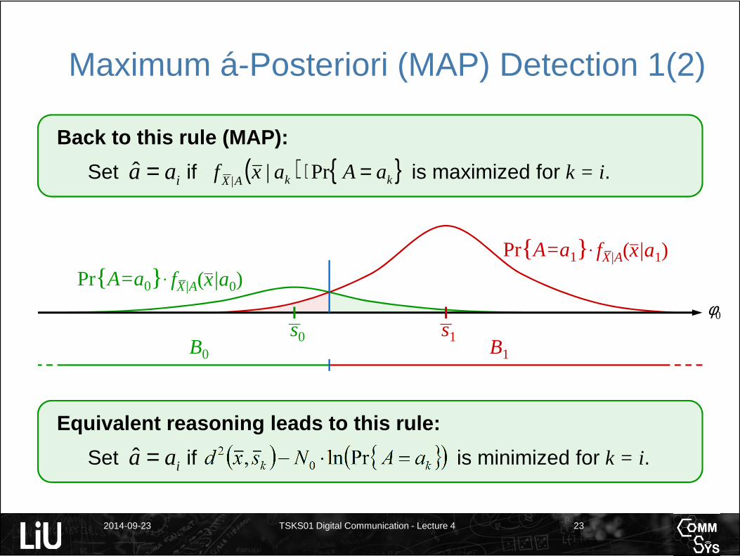
Maximum á-Posteriori (MAP) Detection 1(2)
B1B0
s0 s1
φ0
fX|A(x|a0)Pr{ A=a0} ·fX|A(x|a1)Pr{ A=a1} ·
Back to this rule (MAP):
Set if is maximized for k = i. iaa =ˆ ( ) { }kkAX aAaxf =⋅Pr||
( ) { }( )kk aANsxd =⋅− Prln, 02
Equivalent reasoning leads to this rule:
Set if is minimized for k = i. iaa =ˆ

2014-09-23 TSKS01 Digital Communication - Lecture 4 24
Maximum á-Posteriori (MAP) Detection 2(2)
The borders are still:Straight lines (hyperplanes)Orthogonal to straight lines between signal points.
1 3
3
1
–1
φ0
φ1
2s
0s
1s
B2
B1
B0
But:Borders cut the lines mid-wayonly if the two probabilities are equal.Borders depend on N0.
Note:A signal point may in extreme cases not even be in its own detection region.

2014-09-23 TSKS01 Digital Communication - Lecture 4 25
Special Case: Orthogonal Decision Borders
2s
0s1s
B2
B1B0
3sB3
1,0d
2,1d 2,0d
UB: 0,21,20,1e qqqP ++≤ 1,20,1e qqP +≤Alternative bound:
NN: 1,2e qP ≈ 1,20,1e qqP +≈Alternative approx.:
Exact: 1,20,11,20,1e qqqqP −+=(orthogonal noise components are independent)
=
0
,ji,
2N
dQq jiDefine notation:
22,1
21,0
22,0 ddd +=Pythagoras:
1,2e qP >Lower bound:
2014-09-23 TSKS01 Digital Communication - Lecture 4 26
0θ
α
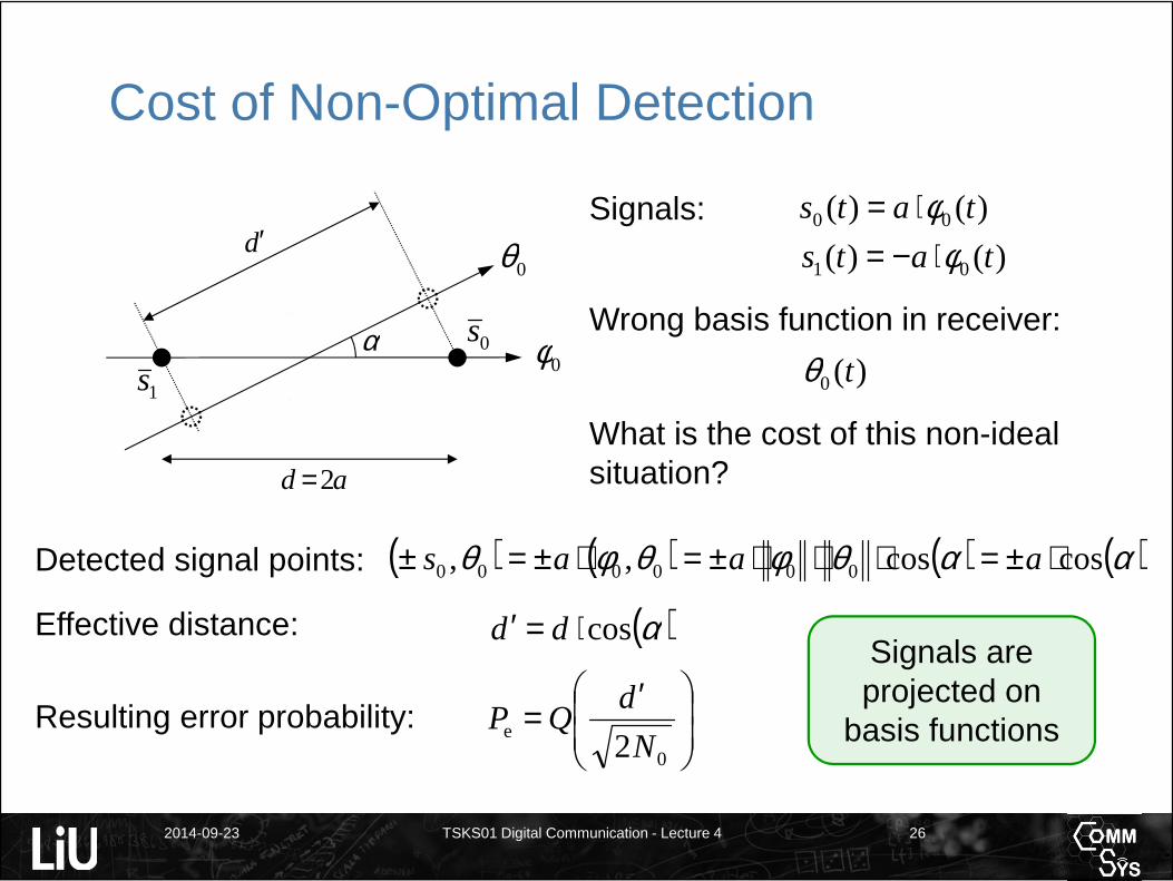
Cost of Non-Optimal Detection
Detected signal points: ( ) ( ) ( ) ( )ααθφθφθ coscos,, 000000 ⋅±=⋅⋅⋅±=⋅±=± aaas
d′Signals: )()( 00 tats φ⋅=
)()( 01 tats φ⋅−=
Wrong basis function in receiver:
)(0 tθ
What is the cost of this non-ideal situation?
0φ0s
1s
ad 2=
( )αcos⋅=′ ddEffective distance:
′=
0
e2N
dQPResulting error probability:
Signals are projected on
basis functions
2014-09-23 TSKS01 Digital Communication - Lecture 4 27
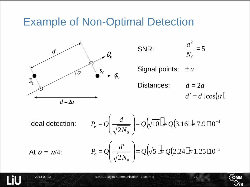
Example of Non-Optimal Detection
( ) ( ) 2
0
e 1025.124.252
−⋅≈≈=
N
dQPAt α = π /4:
Ideal detection: ( ) ( ) 4
0
e 109.716.3102
−⋅≈≈=
N
dQP
d′0θ
0φ0s
1s
ad 2=
α
SNR: 50
2
=N
a
( )αcos⋅=′ dd
Distances: ad 2=
Signal points: a±

www.liu.se