Treasury Options for Fixed Income Asset Managers - CME Group · INTEREST RATES Treasury Options for...
20
INTEREST RATES TreasuryOptionsforFixedIncomeAssetManagers DECEMBER 12, 2013 John W. Labuszewski Michael Kamradt David Reif Managing Director Executive Director Senior Director Research & Product Development 312-466-7469 [email protected] International Development 312-466-7473 [email protected] Interest Rate Products 312-648-3839 [email protected]
Transcript of Treasury Options for Fixed Income Asset Managers - CME Group · INTEREST RATES Treasury Options for...

INTEREST RATES
Treasury Options for Fixed Income Asset Managers
DECEMBER 12, 2013 John W. Labuszewski Michael Kamradt David Reif
Managing Director Executive Director Senior Director
Research & Product Development
312-466-7469
International Development
312-466-7473
Interest Rate Products
312-648-3839
1 Treasury Options for Fixed Income Asset Managers | December 12, 2013 | © CME GROUP
Fixed income asset managers have many strategic
alternatives available to them including the use of
spot, futures and option markets in their pursuit of
investment value (or “alpha’) relative to market
benchmarks. CME Group offers 2-year, 3-year, 5-
year and 10-year Treasury note futures; as well as
“classic” and “Ultra” T-bond futures.
In addition to these highly successful futures
contracts, CME Group offers options exercisable for
these futures contracts. Similar to the underlying
futures, these option contracts offer a high degree of
liquidity, transparency, price discovery and are
accessible through the CME Globex® electronic
trading platform.
This document is intended to provide a review of the
fundamentals of CME Group Treasury options; and,
a discussion of the ways in which these options may
be utilized to manage the risks associated with a
Treasury security investment portfolio.
What is an Option?
Options provide a very flexible structure that may be
tailored to meet the risk management or “alpha”
seeking needs of a portfolio manager. Cash and
futures markets offer portfolio managers the
opportunity to manage risk and opportunity based
upon an assessment of price (or yield) movements.
But options offer further opportunities to conform
the characteristics of a fixed income investment
portfolio to take advantage of additional factors
including convexity, the passage of time and
volatility.
As a first step, let’s get the option basics out of the
way. There are two basic types of options – call and
put options – with two distinct risk/reward
scenarios.
Call option buyers pay a price (in the form of a
“premium”) for the right, but not the obligation, to
buy the instrument underlying the option (in the
case of our discussion, a Treasury futures contract)
at a particular strike or exercise price on or before
an expiration date. Call option sellers (aka, option
“writers” or “grantors”) receive a premium and have
an obligation to sell futures at the exercise price if
the buyer decides to exercise their right.
Put option buyers pay a price for the right, but not
the obligation, to sell a Treasury futures contract at
a particular strike or exercise price on or before an
expiration date. 1 The seller of a put option receives
a premium for taking on the obligation to buy
futures at the exercise price if the put buyer decides
to sell the underlying futures at the exercise price.
Options may be configured as European or American
style options. A European style option may only be
exercised on its expiration date while an American
style option may be exercised at any time up to and
including the expiration date. CME Group offers
options on Treasury futures configured in the
American style as well as flexible or “flex” options
which allow the user to specify non-standardized
expirations or strike prices and which may be
European style.
The purchase of a call option is an essentially bullish
transaction with limited downside risk. If the market
should advance above the strike price, the call is
considered “in-the-money” and one may exercise
the call by purchasing a Treasury futures contract at
the exercise price even when the market rate
exceeds the exercise price.
This implies a profit that is diminished only by the
premium paid up front to secure the option. If the
market should decline below the strike price, the
option is considered “out-of-the-money” and may
expire, leaving the buyer with a loss limited to the
premium.
1 One must exercise some caution when referring to
options on U.S. Treasury futures insofar as these options
terminate trading and expire during the month preceding
the named month. Specifically, options on Treasury
futures terminate trading on the last Friday which
precedes by at least 2 business days the last business
day of the month preceding the option month. Thus, a
“March option” expires in February; a “June option”
expires in May; a “September option” expires in August;
a “December option” expires in November. The named
month is a reference to the delivery period of the futures
contract and not to the option expiration month. Note
that Treasury futures permit the delivery of Treasury
securities on any business day during the contract month
at the discretion of the short. By terminating the option
prior to the named month, traders are afforded the
opportunity to liquidate futures established through an
option exercise and avoid the possibility of becoming
involved in a delivery of Treasury securities against the
futures contract.

2 Treasury Options for Fixed Income Asset Managers | December 12, 2013 | © CME GROUP
The risks and potential rewards which accrue to the
call seller or writer are opposite that of the call
buyer. If the option should expire out-of-the-
money, the writer retains the premium and counts it
as profit. If the market should advance, the call
writer is faced with the prospect of being forced to
sell Treasury futures at the fixed strike price when
prices may be much higher, such losses cushioned
to the extent of the premium received upon option
sale.
The purchase of a put option is essentially a bearish
transaction with limited downside risk. If the market
should decline below the strike price, the put is in-
the-money and one may exercise the put by selling
a Treasury futures contract at the exercise price
even when the market price is less the exercise
price. If the market should advance above the
strike price, the option is out-of-the-money,
implying a loss equal to the premium.
The risks and potential rewards which accrue to the
put writer are opposite that of the put buyer. If the
option should expire out-of-the-money, the writer
retains the premium and counts it as profit. If, the
market should decline, the put writer is faced with
the prospect of being forced to buy Treasury futures
at the fixed strike price when prices are much lower,
such losses cushioned to the extent of the premium
received upon option sale.
While one may dispose of an option through an
exercise or abandonment (expiration sans exercise),
there is also the possibility that one may liquidate a
long/short option through a subsequent
sale/purchase.
Because of the variety of options which are offered,
including puts and calls with varying exercise prices
and expiration dates, one may create an almost
infinite variety of strategies which may be tailored to
suit one’s unique needs. Further, one may deploy a
combination of options to achieve particular risk
management requirements.
Option Pricing
Option pricing is at once one of the most complicated,
but perhaps the most significant, topic which a
prospective option trader can consider. The
importance of being able to identify the "fair value" of
an option is evident when you consider the meaning
of the term fair value in the context of this subject.
A fair market value for an option is such that the
buyer and seller expect to break even in a statistical
sense, i.e., over a large number of trials (without
considering the effect of transaction costs,
commissions, etc.). Thus, if a trader consistently
buys over-priced or sells underpriced options, he can
expect, over the long term, to incur a loss. By the
same token, an astute trader who consistently buys
underpriced and sells over-priced options might
expect to realize a profit.
But how can a trader recognize over- or underpriced
options? What variables impact upon this
assessment? There are a number of mathematical
models which may be used to calculate these figures,
notably including models introduced by
Black-Scholes, Cox-Ross-Rubinstein and Whaley
amongst others. Several factors including the
relationship between market and exercise price,
Pro
fit
Loss
Market Price
Profit/Loss for Call Option
Buy Call Option Sell Call Option
Exercise or
Strike Price
Pro
fit/
Loss
Market Price
Profit/Loss for Put Option
Buy Put Option Sell Put Option
Exercise or
Strike Price

3 Treasury Options for Fixed Income Asset Managers | December 12, 2013 | © CME GROUP
term until expiration, market volatility and interest
rates impact the formula. Frequently, options are
quoted in terms of volatility and converted into
monetary terms with use of these formulae.
The purpose of this section, however, is not to
describe these models but to introduce some of the
fundamental variables which impact an option
premium and their effect. Fundamentally, an option
premium reflects two components: "intrinsic value"
and "time value."
Premium = Intrinsic Value + Time Value
The intrinsic value of an option is equal to its
in-the- money amount. If the option is
out-of-the-money, it has no intrinsic or in-the-money
value. The intrinsic value is equivalent, and may be
explained, by reference to the option's "terminal
value." The terminal value of an option is the price
the option would command just as it is about to
expire.
When an option is about to expire, an option holder
has two available alternatives. On one hand, the
holder may elect to exercise the option or, on the
other hand, may allow it to expire unexercised.
Because the holder cannot continue to hold the option
in the hopes that the premium will appreciate and the
option may be sold for a profit, the option’s value is
limited to whatever profit it may generate upon
exercise.
As such, the issue revolves entirely on whether the
option lies in-the-money or out-of-the-money as
expiration draws nigh. If the option is
out-of-the-money then, of course, it will be
unprofitable to exercise and the holder will allow it to
expire unexercised or "abandon" the option.
An abandoned option is worthless and, therefore, the
terminal value of an out-of-the- money option is zero.
If the option is in-the-money, the holder will profit
upon exercise by the in-the-money amount and,
therefore, the terminal value of an in-the-money
option equals the in-the-money amount.
An option should (theoretically) never trade below its
intrinsic value. If it did, then arbitrageurs would
immediately buy all the options they could for less
than the in-the-money amount, exercise the option
and realize a profit equal to the difference between
the in-the-money amount and the premium paid for
the option.
Time Value
An option contract often trades at a level in excess of
its intrinsic value. This excess is referred to as the
option's "time value" or sometimes as its "extrinsic
value." When an option is about to expire, its
premium is reflective solely of intrinsic value.
But when there is some time until option expiration,
there exists some probability that market conditions
will change such that the option may become
profitable (or more profitable) to exercise. Thus, time
value reflects the probability of a favorable
development in terms of prevailing market conditions
which might permit a profitable exercise.
Generally, an option's time value will be greatest
when the option is at-the-money. In order to
understand this point, consider options which are
deep in- or out-of-the-money. When an option is
deep out-of-the-money, the probability that the
option will ever trade in-the-money becomes remote.
Thus, the option's time value becomes negligible or
even zero.
When an option trends deep in-the-money, the
leverage associated with the option declines.
Leverage is the ability to control a large amount of
resources with a relatively modest investment.
Consider the extraordinary case where a call option
has a strike price of zero. Under these
circumstances, the option's intrinsic value equals the
0
2
4
6
8
10
12
14
16
18
20
22
80
82
84
86
88
90
92
94
96
98
100
102
104
106
108
110
112
114
116
118
120
Option P
rem
ium
Market Price
Intrinsic & Time Value of Call
Intrinsic Value Time Value
Exercise or
Strike Price

4 Treasury Options for Fixed Income Asset Managers | December 12, 2013 | © CME GROUP
outright purchase price of the instrument. There is
no leverage associated with this option and,
therefore, the option trader might as well simply buy
the underlying instrument outright. Thus, there is no
time value associated with the option.
A number of different factors impact on an option on
futures’ time value in addition to the in- or
out-of-the-money amount. These include - (i) term
until option expiration; (ii) market volatility; and (iii)
short-term interest rates. Options exercisable for
actual commodities or actual financial instruments
(i.e., not futures or forwards) are also affected by any
other cash flows such as dividends (in the case of
stock), coupon payments (bonds), etc.
Term until Expiration
An option's extrinsic value is most often referred to as
time value for the simple reason that the term until
option expiration has perhaps the most significant
and dramatic effect upon the option premium. All
other things being equal, premiums will always
diminish over time until option expiration. In order to
understand this phenomenon, consider that options
perform two basic functions - (i) they permit
commercial interests to hedge or offset the risk of
adverse price movement; and (ii) they permit traders
to speculate on anticipated price movements.
The first function suggests that options represent a
form of price insurance. The longer the term of any
insurance policy, the more it costs. The probability
that adverse events may occur is increased as a
function of the term of the option. Hence, the value
of this insurance is greater. Likewise, when there is
more time left until expiration, there is more time
during which the option could potentially move
in-the-money. Therefore, speculators will pay more
for an option with a longer life.
Not only will the time value of an option decline over
time, but that time value "decay" or "erosion" may
accelerate as the option approaches expiration. But
be aware that accelerating time value decay is a
phenomenon that is characteristic of at- or
near-the-money options only. Deep in- or
out-of-the-money options tend to exhibit a linear
pattern of time value decay.
Volatility
Option holders can profit when options trend
into-the-money. If market prices have a chance, or
probability, to move upwards by 10%, option traders
may become inclined to buy call options. Moreover, if
market prices were expected to advance by 20% over
the same time period, traders would become even
more anxious to buy calls, bidding the premium up in
the process.
It is not always easy to predict the direction in which
prices will move, but it may nonetheless be possible
to measure volatility. Market volatility is often
thought of as price movement in either direction,
either up or down. In this sense, it is the magnitude,
not the direction, of the movement that counts.
Standard deviation is a statistic that is often
employed to measure volatility. These standard
deviations are typically expressed on an annualized
basis. E.g., you may see a volatility quoted at 10%,
0123456789
101112131415161718192021
80 81 82 83 84 85 86 87 88 89 90 91 92 93 94 95 96 97 98 99 100 101 102 103 104 105 106 107 108 109 110 111 112 113 114 115 116 117 118 119 120
Option P
rem
ium
Market Price
Intrinsic & Time Value of Put
Intrinsic Value Time Value
Exercise or
Strike Price
0123456789
101112131415161718192021
80
82
84
86
88
90
92
94
96
98
100
102
104
106
108
110
112
114
116
118
120
Option P
rem
ium
Market Price
Time Value Decay
3 Mths til Expiration 2 Mths til Expiration
1 Mth til Expiration Value at Expiration
Exercise or
Strike Price

5 Treasury Options for Fixed Income Asset Managers | December 12, 2013 | © CME GROUP
15%, 20%, etc. The use of this statistic implies that
underlying futures price movements may be modeled
by the "normal price distribution." The popular Black
Scholes and Black option pricing models are, in fact,
based on the assumption that movements in the
instrument underlying an option may be described by
reference to the normal pricing distribution. The
normal distribution is represented by the familiar “bell
shaped curve.”
To interpret a volatility of 6%, for example, you can
say with an approximate 68% degree of confidence
that the price of the underlying instrument will be
within plus or minus 6% (=1 standard deviation) of
where it is now at the conclusion of one year. Or,
with a 95% degree of confidence that the price of the
underlying instrument will be within plus or minus
12% (=2 x 6% or 2 standard deviations) of where
the price lies now at the conclusion of a year. A good
rule of thumb is that the greater the price volatility,
the more the option will be worth.
One may readily calculate an historic or realized
volatility by taking the standard deviation of day-to-
day returns in the market of interest. One may
sample these returns over the past 30, 60, 90, 180
days or some other period of interest and express the
resulting number of an annualized basis. The implicit
assumption is that movements over the past X
number of days may be reflective of future market
movements.
But the aggregate expectations of market participants
with respect to future volatility may be at odds with
past volatility. Thus, traders often reference “implied
volatilities” or the volatility that is implicit in the level
of an option premium as traded in the market.
As suggested above, there are various mathematical
pricing models available which may be used to
calculate the fair value of the option premium as a
function of the underlying futures price (U), strike
price (S), term until expiration (t), volatility (v) and
short-term interest rates (r).
������� = �(, �, , �, �)
The underlying market price, strike price, term and
short-term rates are readily observable. Further, the
option premium trading in the marketplace may also
be readily observable. This leaves volatility as the
least readily observable and most abstract of the
necessary variables. But one may solve the
mathematical pricing model to find volatility or
“implied volatility” as a function of the observed
premium and the other variables.
� = �(�������,, �, , �)
Referring to the table in the appendix below, we note
that the implied volatilities (IVs) may be quite
different amongst options that share a common
underlying instrument and expire on the same date.
E.g., the near-the-money 127 December 2013 put
had an IV=4.89% while the out-of-the-money 126
put had an IV=5.34%.
Traders frequently impute different values to options
based on their subtly different investment attributes.
Options on Treasury futures are most heavily utilized
by institutional traders who often deploy these
options for risk management purposes. They tend to
value less expensive out-of-the-money puts as a
means of buying price protection as discussed in
more detail above. Thus, they may bid up the value
of less expensive out-of-the-money puts, particularly
where they perceive a high risk of rising rates and
falling Treasury prices.
This may create a pattern known as the option skew
or “smile” by reference to the fact that the graphic
display of this information sometimes resembles a
smile.
Treasury rates had been generally drifting higher as
of October 2013 with much anticipation that the
Treasury might begin to “taper” its quantitative
0%
1%
2%
3%
4%
5%
6%
7%
124-1
6
125.0
0
125-1
6
126.0
0
126-1
6
127-0
0
127-1
6
128-0
0
128-1
6
129-0
0
129-1
6
Strike Prices
10-Year T-Note Option Skew(Dec-13 Options as of 10/17/13)
Call Options Put Options

6 Treasury Options for Fixed Income Asset Managers | December 12, 2013 | © CME GROUP
easing programs, leading to higher rates and lower
prices.
This is reflected in the skew such that low-struck puts
were generally bid up, resulting in higher implied
volatilities. Calls with the same strike likewise
displayed progressively higher IVs as a result of “put-
call parity” phenomenon. 2
Short-Term Rates
When someone invests in a business venture of any
sort, some positive return typically is expected.
Accordingly, when an option exercisable for a futures
contract is purchased there is an investment equal to
the premium. To the extent that the option is paid
for up front and in cash, a return is expected on the
investment.
This implies that premiums must be discounted to
reflect the lost opportunity represented by an
investment in options. When the opportunity cost
rises, as reflected in the rate at which funds may
alternately be invested on a short-term basis, the
price of an option is discounted accordingly. When
the opportunity cost decreases, the premium
appreciates.
These remarks must be qualified by the following
considerations. First, the effect described is
applicable only to options on futures and not to
options exercisable for actual instruments. In fact,
rising short-term rates will tend to increase call
2 Put-call parity suggests that if puts and calls of the same
strike did not trade with approximately equal IVs, an
arbitrage opportunity would arise. The execution of such
an arbitrage would cause these IVs to align in equilibrium.
Specifically, if a call were to trade significantly “richer”
than a put with identical strikes, as measured by their
respective IVs, one might pursue a “conversion”
strategy. This entails the sale of the call and purchase of
the put, creating a “synthetic short futures” position.
This is hedged by the simultaneous purchase of futures,
effectively locking in an arbitrage profit. A “reverse
conversion” or “reversal may be pursued if the put were
trading richer than the call with the same strike. This
entails the sale of the put and purchase of the call,
creating a “synthetic long futures” position. One hedges
with the simultaneous sale of futures, locking in an
arbitrage profit. Trader will continue to execute these
traders until they have restored a market equilibrium
and it becomes unprofitable to continue placing these
strategies, after considering the attendant transaction
costs.
premiums and decrease put premiums for options
exercisable for actual instruments.
Secondly, these remarks apply holding all other
considerations equal. But of course, we know that all
else is never held equal. For example, if short-term
rates are rising or falling, this suggests that bond
futures prices will be affected. Of course, this
consideration will also have an impact, often much
greater in magnitude, than the impact of fluctuating
short- term rates.
Delta
When the price of the underlying instrument rises,
call premiums rise and put premiums fall. But by
how much? The change in the premium relative to
the change in the underlying commodity price is
measured by a common option statistic known as
"delta."
Delta is generally expressed as a number from zero
to 1.0. Deep in-the-money deltas will approach 1.0.
Deep out-of-the- money deltas will approach zero.
Finally at- or near-the-money deltas will run at about
0.50.
It is easy to understand why a deep in- or
out-of-the-money option may have a delta equal to
1.0 or zero, respectively. A deep in-the-money
premium is reflective solely of intrinsic or
in-the-money value. If the option moves slightly
more or less in-the-money, its time value may be
unaffected. Its intrinsic value, however, reflects the
relationship between the market price and the fixed
strike price, hence, a delta of 1.0.
Delta
Deep In-the-Money ����1.00
At-the-Money ���� 0.50
Deep Out-of-the-Money ���� 0.00
At the other extreme, a deep out-of-the-money
option has no value and is completely unaffected by
slightly fluctuating market prices. Hence, a delta of
zero.
A call delta of 0.50 suggests that if the value of the
underlying instrument advances by $1, the premium
will advance by 50 cents. A put delta of 0.50
suggests that if the value of the underlying

7 Treasury Options for Fixed Income Asset Managers | December 12, 2013 | © CME GROUP
instrument advances by $1, the premium will fall by
50 cents.
Note that the delta of a bullish option, i.e., a long call
or short put, is often assigned a positive value. On
the other hand, an essentially bearish option, i.e., a
long put or short call, is often assigned a negative
value. This convention facilitates summation of the
deltas of all options in a complex position (based
upon the same or similar underlying instrument) to
identify the net risk exposure to price or yield
fluctuations.
Delta is a dynamic concept. It will change as the
market price moves upwards or downwards. Hence,
if an at-the-money call starts trending
into-the-money, its delta will start to climb. Or, if the
market starts falling, the call delta will likewise fall.
The table in our appendix below provides the delta
as well as other statistics for a wide variety of
options exercisable for 10-Year U.S. Treasury note
futures contracts. This data represents intra-day
values sampled as of October 17, 2013 in the
December 2013 options. 3
E.g., the at- or nearest-to-the-money December
2013 call option was struck at 127-00/32nds while
December 2013 futures was quoted at 126-
26+/32nds. It was bid at a premium of 0-45/64ths
with a delta of 0.47. This suggests that if the
market were to advance (decline) by one point (i.e.,
1 percent of par) the premium would be expected to
advance (decline) by approximately one-half of a
point (holding all else constant).
Thus, delta advances as the option moves in-the-
money and declines as the option moves out-of-the-
3 Note that 10-year Treasury note futures contracts are
based upon a $100,000 face value contract size. They
are quoted in percent of par and 32nds of 1% of par with
a minimum price increment or “tick” of 1/64th or $15.625
(=1/64th of 1% of $100,000). Thus, a quote of 128-16
represents 128 + 16/32nds or 128.50% of par. A
futures quote of 128-165 means 128 + 16/32nds + ½ of
1/32nd. This equates to 128.515625% or par. Options
on 10-year Treasury note futures contracts call for the
delivery upon exercise of one $100,000 face value 10-
year T-note futures contract. They are quoted in percent
of par in increments of 1/64th of 1% of par or $15.625
(=1/64th of 1% of $100,000). Thus, one might see a
quote of 1-61/64ths which equates to 1.953125% of par.
money. This underscores the dynamic nature of
delta.
“Greek” Statistics
In addition to movement in the underlying market
price (as measured by delta), other factors impact
significantly upon the option premium, notably
including time until expiration and marketplace
volatility.
A number of exotic “Greek” statistics including delta,
gamma, vega and theta are often referenced to
measure the impact of these factors upon the option
premium. Underlying price movement stands out as
perhaps the most obvious factor impact option
premiums and we have already discussed delta as
the measure of such impact. Let’s consider other
statistics including gamma, vega and theta.
“Greek” Option Statistics
Delta
Measures expected change in premium
given change in PRICE of instrument
underlying option
Gamma
Measures change in DELTA given change in
PRICE of instrument underlying option, i.e.,
“delta of the delta” measuring CONVEXITY
Vega
Measures expected change in option
premium given change in VOLATILITY of
instrument underlying option
Theta Measures expected change in option
premium given forward movement of TIME
Gamma may be thought of as the "delta of the
delta." Gamma measures the expected change in
the delta given a change in the underlying market
price. Gamma is said to measure a phenomenon
known as "convexity." Convexity refers to the shape
of the curve which depicts the total value of an
option premium over a range in possible underlying
market values. The curvature of that line is said to
be convex, hence the term convexity.
Convexity is a concept which promises to benefit
traders who purchase options to the detriment of
those who sell or write options. Consider that as the
market rallies, the premium advances at an ever
increasing rate as the delta itself advances. Thus,
the holder of a call is making money at an increasing
or accelerating rate. But if the market should fall,
the call holder is losing money but at a decelerating
rate.

8 Treasury Options for Fixed Income Asset Managers | December 12, 2013 | © CME GROUP
E.g., on October 17, 2013, the delta for a December
2013 call option on 10-Year T-note futures, struck at
127-00/32nds (essentially at-the-money with
December futures trading at 126-26+/32nds) was
0.47. It had a gamma of 0.2535 suggesting that if
the underlying futures price were to move upwards
(downwards) by 1 percent of par, the value of delta
would move upwards (downwards) by about 0.2535.
If the call buyer is making money at an accelerating
rate and losing money at a decelerating rate, the call
writer is experiencing the opposite results. Gamma
tends to be highest when an option is at- or near-to-
the-money. But gamma declines as an option
trends in- or out-of-the-money.
Theta and vega are likewise greatest when the
market is at or reasonably near to the money.
These values decline when the option goes in- or
out-of-the-money as discussed below. Thus,
convexity as measured by gamma works to the
maximum benefit of the holder of at-the-money
options.
Theta measures time value decay or the expected
decline in the option premium given a forward
movement in time towards the ultimate expiration
date of the option, holding all other variables (such
as price, volatility, short-term rates) constant. Time
value decay and the degree to which this decay or
erosion might accelerate as the option approaches
expiration may be identified by examining the
change in the theta.
E.g., our December 2013 127-00 call had a theta of
-0.0107. This suggests that over the course of one
(1) day, holding all else equal, the value of this call
option may fall 0.0107 percent of par. This equates
to 0.685/64ths (=0.0107 x 64) or about $10.70 per
$100,000 face value unit. Thus, the premium is
expected to decline from the current value of 0-
45/64ths to approximately 44/64ths over the course
of a single day, rounding quotes to the nearest
integral multiple of the tick size.
Note that we are quoting a theta in percent of par
over the course of 1 calendar day. It is also
common to quote a theta over the course of seven
(7) calendar days. One must be cognizant of the
references that are being made in this regard.
Theta is a dynamic concept and may change
dramatically as option expiration draws nigh. At- or
near-to-the-money options experience rapidly
accelerating time value decay when expiration is
close. Away-from-the-money options experience
less time value decay as in-and out-of-the-money
options have less time value than do comparable at-
or near-the-money options.
Thetas associated with moderately in- or out-of-the-
money options may be relatively constant as
expiration approaches signifying linear decay
characteristics. Deep in- or out-of-the-money
options will have very little or perhaps no time
value. Thus, the theta associated with an option
whose strike is very much away from the money
may "bottom-out" or reach zero well before
expiration.
Time value decay works to the benefit of the short
but to the detriment of the long. The same options
which have high thetas also have high gammas.
Convexity as measured by gamma works to the
detriment of the short and to the benefit of the long.
Near-the-money options will have high thetas and
high gammas. As expiration approaches, both theta
(measuring time value decay) and gamma
(measuring convexity) increase.
Thus, it becomes apparent that you "can't have your
cake and eat it too." In other words, it is difficult, if
not impossible, to benefit from both time value
decay and convexity simultaneously.
Vega measures the expected change in the premium
given a change in marketplace volatility. Normally,
vega is expressed as the change in the premium
given a one percent (1.0%) movement in volatility.
E.g., our December 2013 127 call had a vega of
0.1579. This suggests that its premium of 45/64ths
might fluctuate by approximately 10/64ths
(=0.1579 x 64) or about $157.90 per $100,000 face
value unit, if volatility were to move by 1% from the
current implied volatility of 4.99%.
Vega tends to be greatest when the option is at- or
reasonably near-to-the-money. In- and out-of-the-
money options have generally lower vegas.
However, this effect is not terribly great. Note that
vega tends to fall, rather than rise, as a near-to-the-
money option approaches expiration. This is unlike
9 Treasury Options for Fixed Income Asset Managers | December 12, 2013 | © CME GROUP
the movement of theta and gamma which rise as
expiration draws near.
Volatility and convexity are highly related properties.
This can be understood when one considers that it is
only when the market is moving, or when the
market is volatile, that the effects of convexity are
observed.
Remember that when you buy an option, convexity
works to your benefit no matter whether underlying
price movements are favorable or not. If the market
moves against you, you lose money at a
decelerating rate. If the market moves with you,
you make money at an accelerating rate. Thus, the
prospect of rising volatility is generally accompanied
by beneficial effects from convexity (at least from
the long's standpoint).
Earlier we suggested that it is generally impossible
to enter an option strategy in which both time value
decay and convexity worked to your benefit
simultaneously. Paradoxically, it may be possible to
find option strategies where the prospect of rising
volatility and time value decay work for you
simultaneously (although convexity will work against
you).
This is possible because vega falls as expiration
approaches while theta and gamma rise. E.g., one
might buy a long-term option experiencing the ill
effects of time value decay while selling a shorter-
term option which benefits from time value decay.
The benefits associated with the short-term option
will outweigh the disadvantages associated with the
longer-term option. And, the strategy will generally
benefit from the prospect of rising volatility as the
long-term option will have a higher vega than will
the short-term option.
Putting It All Together
Options are strongly affected by the forces of price,
time and volatility/convexity. (We often consider
convexity and volatility to be one in the same
property for reasons discussed above.) "Exotic"
option statistics such as delta, gamma, theta and
vega are quite useful in measuring the effects of
these variables.
As a general rule, when you buy an option or enter
into a strategy using multiple options where you
generally buy more than you sell, convexity and the
prospect of rising volatility work to your benefit.
Time value decay generally works against you in
those situations. When you sell options or enter into
strategies where you are generally selling more
options than you buy, convexity and the prospect of
rising volatility will work against you although time
value decay will work to your benefit.
Earlier we had suggested that essentially bullish
options including long calls and short puts are
frequently assigned positive deltas. Essentially
bearish options including long puts and short calls
are likewise often assigned negative values. This
facilitates summation of the “net delta” associated
with a complex option position (based upon the
same or similar underlying instruments).
Likewise, we often attach positive or negative values
to gamma, theta and vega. To the extent that rising
gammas and vegas benefit long option holders, we
assign positive gammas and vegas to long calls and
puts; and, negative gammas and vegas to short
calls and puts. On the other hand, rising thetas
benefit shorts to the detriment of longs. Thus, long
puts and calls are frequently assigned negative
thetas while shorts are assigned positive thetas.
The key point is that these variables - price, time
and volatility - do not operate independently one
from the other. Price may generally be considered
the most important of these variables and will tend
to dictate whether time value decay is more or less
important than convexity and rising volatility. One
can use this information to good effect when
formulating a hedging strategy using options.
Measuring Portfolio Risk
Now that we have established a foundation for
understanding the pricing of options, let’s explore
how options may be used to hedge the risks
associated with fixed income investment portfolios.
But, just as we measure the risks uniquely
associated with options by reference to the
“Greeks,” we must likewise establish a framework
for measuring risks associated with fixed income
securities. In the fixed income markets, one
generally measures portfolio risk by reference to
duration or “basis point value” (BPV).

10 Treasury Options for Fixed Income Asset Managers | December 12, 2013 | © CME GROUP
Duration is a concept that was originated by the
British actuary Frederick Macauley. Mathematically,
it is a reference to the weighted average present
value of all the cash flows associated with a fixed
income security, including coupon income as well as
the receipt of the principal or face value upon
maturity.
E.g., the most recently issued or “on-the-run” 10-
year Treasury note as of September 30, 2013 was
the 2-½% security maturing August 15, 2023. Its
duration was equal to 8.662 years. This suggests
that if yields were to advance by 100 basis points
(or “bps”), the price of the security should decline by
approximately 8.662%.
Basis point value (BPV) is a concept that is closely
related to modified duration. The BPV measures the
expected change in the price of a security given a 1
basis point (0.01%) change in yield. It may be
measured in dollars and cents based upon a
particular face value security, commonly $1 million
face value. It is sometimes also referred to as the
“dollar value of an 01” or simply “DV of an 01.”
On-the-Run Treasury Notes & Bonds (9/30/13)
Tenor Coupon Maturity Modified
Duration
BPV (per
million)
2-Year ¼% 9/30/15 1.990 $199
3-Year 7/8% 9/15/16 2.915 $294
5-Year 1-3/8% 9/30/18 4.813 $481
7-Year 2% 9/30/20 6.499 $650
10-Year 2-½% 8/15/23 8.662 $861
30-Year 3-5/8% 8/15/43 17.999 $1,789
E.g., the on-the-run 10-year T-note had a basis
point value of $861 per $1 million face value unit, as
of September 30, 2013. This implies that if yields
were to advance by 1 basis point, the price of a $1
million face value unit of the security might decline
by $861.
In particular, we compare how futures, puts and
calls may be used to hedge a fixed income
investment exposure. In the process, we might ask:
what hedging strategy is best under what kind of
market conditions? In other words, can we select an
option strategy which may be well matched to
prospective market conditions?
Futures Hedge
In order to provide a comparison of various hedging
strategies with the use of options, let us review the
efficacy of a short futures hedge against a long
Treasury portfolio. This is intended to serve as a
“baseline” against which the effect of option
strategies may be compared.
Interest rate futures are frequently utilized to hedge,
or more specifically, to adjust the average weighted
duration of fixed income investment portfolio. In
particular, one might increase risk exposure as
measured by duration in anticipation of rate declines
(price advances); or, decrease duration when rate
increases (price decline) are forecast. One may buy
futures to extend duration; or, sell futures to reduce
duration.
E.g., consider a hypothetical fixed income portfolio
valued at $100 million with a weighted average
duration of 8 years. In anticipation of increasing
rates and declining prices, the asset manager
decides to execute a temporary tactical shortening
of portfolio duration from 8 years to 6 years.
This may be executed by selling CME Group
Treasury note futures. While Treasury futures are
available based upon all the major tenures extended
out on the yield curve, 10-year Treasury note
futures will have an effective duration closest to the
current portfolio duration of 8 years. The
appropriate number of futures to sell, or the “hedge
ratio” (HR), may be calculated using the following
formula.
�� =�������� − ���������������� � � !�"#$��%$&'$ ÷ �!�"��)*+��) �,
Where Dtarget is the target duration; Dcurrent is the
current duration. CFctd is the conversion factor of
the security that is cheapest-to-deliver against the
particular futures contract that is being used.
BPVportfolio represents the basis point value of the
portfolio. Finally, BPVctd is the basis point value of
the cheapest-to-deliver security. 4
4 Treasury note and bond futures contracts permit the
delivery of a variety of Treasury securities within a
certain maturity window, at the discretion of the short.
E.g., the 10-year T-note futures contract permits the
delivery of T-notes with a remaining maturity between 6-
1/2 to 10 years. This includes a rather wide variety of

11 Treasury Options for Fixed Income Asset Managers | December 12, 2013 | © CME GROUP
E.g., assume that the $100 million portfolio had a
BPV equal to $80,000. As of October 17, 2013, the
cheapest-to-deliver (CTD) security vs. December
2013 10-year T-note futures was the 2-1/8%
coupon security maturing in August 31, 2020. This
note had a conversion factor (CF) of 0.7939 with a
BPV of $64.40 per a $100,000 face value unit,
corresponding to the deliverable quantity against a
single futures contract.5 Using these inputs, the
appropriate hedge ratio may be calculated as short
248 futures contracts.
�� = �6 − 88 � � /$80,000 ( 2$64.400.793989
� �247;���<<247�� ���=
By selling 247 Ten-Year T-note futures against the
portfolio, the asset manager may be successful in
pushing his risk exposure as measured by duration
from 8 to 6 years.
Sell futures � Reduce portfolio risk as
measured by duration
securities with varying coupons and terms until maturity.
Because these securities may be valued at various
levels, the contract utilized a Conversion Factor (CF)
invoicing system to determine the price paid by long to
compensate the short for the delivery of the specific
security. Specifically, the principal invoice amount paid
from long to short upon delivery of securities is
calculated as a function of the futures price multiplied by
the CF. Technically, CFs are calculated as the price of
the particular security as if they were yielding the
“futures contract standard” of 6%. The system is
intended to render equally economic the delivery of any
eligible for delivery security. However, the mathematics
of the CF system is such that a single security tends to
stand out as most economic or cheapest-to-deliver
(CTD) in light of the relationship between the invoice
price of the security vs. the current market price of the
security. Typically, long duration securities are CTD
when prevailing yields are in excess of the 6% futures
market standard; while short duration securities are CTD
when prevailing yields are less than 6%. It is important
to identify the CTD security because futures will tend to
price or track or correlate most closely with the CTD. 5 These relationships are dynamic and subject to constant
change. In particular, the BPV associated with any
portfolio or security will change of its own accord in
response to fluctuating yield levels. As a rule, an asset
manager might wish to review the structure of a hedge
transaction upon a 20 basis point movement in
prevailing yields. Further, the CTD will change as a
function of changing yield levels, particularly when
prevailing yields are in the vicinity of the 6% futures
contract standard which may be regarded as an inflection
point of sorts. However, this information may be found
at www.cmegroup.com.
If yields advance by 100 bps, the value of the
adjusted portfolio may decline by approximately 6%
or $6 million. But this is preferable to a possible $8
million decline in value if the asset manager
maintained the portfolio duration at the original
benchmark duration of 8 years. Thus, the asset
manager preserved $2 million in portfolio value.
Of course, the asset manager may readily
accomplish the same objective simply by selling off a
portion of the portfolio holdings in favor of cash.
But Treasury futures tend to be more liquid than the
cash markets. Moreover, the futures hedge allows
the asset manager to maintain his current holdings
while adjusting duration exposures quickly and at
minimal costs.
In this example, we assume that the asset manager
hedges only a portion of his risk (a “partial hedge”).
This assumption is realistic to the extent that the
performance of fixed income portfolio managers is
often assessed relative to a “benchmark” index.
E.g., while there are many suitable fixed income
indexes, the Barcap U.S. Aggregate Bond Index
stands out as a popular example. Thus, a fixed
income portfolio manager may generally conform
the characteristics of his portfolio to the benchmark
(“core” or “beta” returns) but attempt to enhance
returns (or add “alpha”) above those benchmark
returns.
But the manager may have limited discretion to alter
the composition of the portfolio. E.g., assume our
portfolio manager has discretion to decrease
duration from 8 years to 6 years in anticipation of
rising rates; or, to increase duration from 8 years to
10 years in anticipation of falling rates. While the
-25.00
-20.00
-15.00
-10.00
-5.00
0.00
5.00
10.00
15.00
20.00
25.00
80
81
82
83
84
85
86
87
88
89
90
91
92
93
94
95
96
97
98
99
100
101
102
103
104
105
106
107
108
109
110
111
112
113
114
115
116
117
118
119
120
Retu
rn
Market Prices
Hedged with Short Futures
Fixed Income Portfolio Fully Hedged
Partially Hedged
Prices Decline
& Yields
Prices Advance
& Yields Decline

12 Treasury Options for Fixed Income Asset Managers | December 12, 2013 | © CME GROUP
prospect of increasing duration and accepting more
risk seems to run contrary to the classic concept of a
“hedge,” it is nonetheless consistent with the
concept of “managing risks” in pursuit of enhanced
returns.
In the interest of establishing a “baseline” example,
however, consider the possibility of a hedge that
reduces portfolio risk to an absolute minimum.
E.g., if the hedging objective was to push duration
from 8 to 0 years, i.e., to be “fully hedged,” our
portfolio manager might have sold 992 futures.
�� = �0 − 88 � � /$80,000 ( 2$64.400.793989
� �986;���<<986�� ���=
While perhaps not typical in practice, this fully
hedged strategy could have been used effectively to
push duration to essentially zero. This is analogous
to liquidating the longer term securities in the
portfolio and replacing them with very short-term
money market instruments. As such, the portfolio
manager might expect to earn a return that
approximates short-term yields.
Buying Protection with Puts
The idea behind the purchase of puts is to
compensate loss associated with the potentially
declining value of bond prices (rising yields) with the
rising intrinsic value of the puts. As market prices
decline, puts will go deeper and deeper in-the-
money, permitting the put holder to exercise the
options for a profit.
If the market should rally instead, the puts go out-
of-the-money. Having paid the option premium up
front, however, the put holder’s loss is limited to
that premium. Any advance in the underlying
market price (decline in yields) would represent a
profit in the value of the fixed income portfolio,
limited only to the extent of the premium forfeit up
front to purchase the puts.
E.g., our fixed income asset manager holding a $100
million Treasury portfolio with a duration of 8 years
might elect to purchase 986 at-the-money put
options. Note that this example assumes that our
asset manager buys puts using the “fully hedged”
ratio as described above.
If market prices should decline as yields advance,
the portfolio suffers a loss. However, that loss is
offset to the extent that the long put options are
going in-the-money and will permit a profitable
exercise at or before expiration. The long puts are
exercised by selling futures at the put strike despite
the fact that the market has declined below the
strike price. If the hedge was ratioed as described
above, it is as if the asset manager locked in a “floor
price” for his portfolio.
If, on the other hand, the market should advance
above the put strike price as yields decline, the
options will go out-of-the-money and eventually
expire worthless. As such, the asset manager has
forfeit the premium paid up front to secure the
options. However, this payment may be offset and
more by an advance in the portfolio value.
As such, the long put hedge allows one to lock-in a
floor return while still retaining a great deal of the
upside potential associated with a possibly favorable
market swing, limited to the extent that you pay the
premium associated with the purchase of the put
options up front.
Buy put
options �
Lock in “floor return” &
retain upside potential
Option premiums are, of course, impacted by a
variety of factors including the movement of price,
time and volatility. So while the purchase of put
options in the context of a hedging application
-25.00
-20.00
-15.00
-10.00
-5.00
0.00
5.00
10.00
15.00
20.00
25.00
80
81
82
83
84
85
86
87
88
89
90
91
92
93
94
95
96
97
98
99
100
101
102
103
104
105
106
107
108
109
110
111
112
113
114
115
116
117
118
119
120
Retu
rn
Market Prices
Buying Put Protection
Fixed Income Portfolio Put Protection
Prices Decline
& Yields
Prices Advance
& Yields Decline

13 Treasury Options for Fixed Income Asset Managers | December 12, 2013 | © CME GROUP
reduces price risks, it also entails the acceptance of
other types of risk uniquely applicable to options.
Still, price impact is the foremost of these factors.
The degree to which you immediately reduce price
risk may be found by reference to the put delta. In
our example above, we assumed that our asset
manager buys at- or near-the-money put options
with a delta of approximately 0.50. As such, we
effectively reduce the immediate or near-term price
risk by a factor of about one-half (using the
appropriate futures hedge ratio).
But delta is a dynamic concept. If the market falls
and the put option goes in-the-money, the delta will
get closer to 1.0. If the market rises and the put
option goes out-of-the-money, the delta gets closer
to zero. An in-the-money put with a delta of 0.60
suggests an effective 60% reduction in price risk
while the use of an out-of-the-money option with a
delta of 0.40 suggests a 40% reduction in price risk.
The dynamic nature of delta represents convexity.
Convexity, or the change in delta quantified by
gamma, benefits the holder of a put insofar as it
promises more protection in a bear market when
you need more protection; and, less protection in a
bull market when you would prefer less protection.
Unfortunately, you pay for convexity by accepting
negative time value decay.
As expiration approaches, a near-to-the-money
option will exhibit more and more time value decay
or "accelerating" time value decay or erosion. It is
interesting that the same options which experience
high and rising convexity (near-term,
near-the-moneys) also experience high and rising
thetas. Barring a mispricing, it is impossible to
experience both a positive gamma and theta
(change in the premium given the elapse of time)
when trading options.
Thus, you must ask yourself whether market
conditions are likely to be volatile and, therefore,
you should take advantage of convexity by buying
options. Or, will market conditions remain
essentially stable, recommending a strategy of
taking advantage of time value decay by selling
options?
Yield Enhancement with Calls
If you believe that the market is basically stable,
you might pursue a "yield enhancement" or "income
augmentation" strategy by selling call options
against a long cash or spot position. This is also
known as "covered call writing" in the sense that
your obligation to deliver the instrument underlying
the option as a result of writing a call is "covered" by
the fact that you may already be long the
instrument or similar instruments.
In these examples, of course, we assume that our
portfolio manager owns Treasury securities and
trades options exercisable for Treasury futures.
While Treasury futures call for the delivery of
Treasury securities, the two instruments are, of
course, different. But to the extent that Treasury
securities and futures perform similarly in response
to dynamic market conditions, one may be a
reasonable proxy for the other. Hence, the term
“covered” call writing remains appropriate.
E.g., let’s revisit our example of the asset manager
who holds $100 million of Treasury securities with
an average weighted duration of 8 years. Assume
that our manager sells 986 at-the-money call
options (using the “fully hedged” futures hedge
ratio).
If the market remains stable or declines (on
advancing yields) below the strike price, then the
short calls fall out-of-the-money and eventually
expire worthless. As such, the asset manager
retains the full value of the option premium received
up front upon sale. The receipt of this premium
serves to enhance portfolio returns in a neutral or
bear market.
But if the market should advance above the call
strike price, the options will go in-the-money. As
such, they may be exercised, compelling the asset
manager to sell futures at the fixed strike price even
though market prices may be trading at higher
levels. This implies a loss which offsets the
advancing value of the Treasury portfolio.
Still, the initial receipt of the option premium
ensures that a positive return is realized
nonetheless. Thus, the covered call strategy implies
that you lock-in a ceiling return, limiting your ability
to participate in any upside potential. The covered

14 Treasury Options for Fixed Income Asset Managers | December 12, 2013 | © CME GROUP
call writer is compensated, however, to the extent
that he receives the option premium which at least
partially offsets downside losses.
While a long put hedge enables you to take
advantage of convexity albeit while suffering the ill
effects of time value decay. The short call hedge is
just the opposite insofar as it allows you to capitalize
on time value decay while suffering from the
potentially ill effects of convexity.
Sell call
options �
Enhances income in neutral
market & lock-in ceiling return
Convexity and volatility are closely related concepts.
It is only when the market is volatile, when it is
moving either up or down, that the effects of
convexity are actually observed. If the market is
moving and volatility is rising, the short calls may
rise in value, resulting in loss.
If the market should advance, the calls will go
in-the-money, the delta approaching 1.0. The
growing intrinsic value of the calls presumably
offsets profit in the rising value of the cash security
resulting in an offset.
Fortunately, this return is positive by virtue of the
initial receipt of the option premium. If the market
should decline, the calls go out-of-the-money,
eventually expiring worthless as the delta
approaches zero. Still, the hedger is better off
having hedged by virtue of the receipt of the
premium up front.
The short call hedge works best when the market
remains basically stable. In this case, time value
decay results in a gradual decline in the premium.
Thus, you "capture" the premium, enhancing yield.
Matching Strategy with Forecast
Note that by buying puts against a long cash
portfolio, the risk/reward profile associated with the
entire position strongly resembles that of an outright
long call. As such, this strategy is sometimes
referred to as a "synthetic long call." Likewise, the
combination of selling calls against a long cash
currency portfolio will strongly resemble the outright
sale of a put. Thus, we sometimes refer to this
strategy as a "synthetic short put."
Many textbooks draw a strong distinction between
hedging or risk-management and speculative
activity. We are not so sure that this distinction is
warranted in the context of fixed income portfolio
management when the portfolio manager’s objective
is to seek enhanced returns over that of some
“benchmark” or “bogey,” as opposed to an objective
of simply matching the returns on the benchmark on
a passive basis.
The same factors which might motivate a speculator
to buy calls might motivate a hedger to buy puts
against a cash portfolio to generate alpha as yields
rise. Likewise, the same factors which might
motivate a speculator to sell puts might motivate a
hedger to sell calls against his cash portfolio to
enhance yield or “alpha” in a stable or low volatility
market environment.
How might we define hedging versus speculative
activity? Clearly a speculator is someone who might
use futures and options in an attempt to make
money. A hedger is someone who might use futures
and options selectively in an attempt to add alpha
and who already holds a cash position. Perhaps this
distinction does not conform with the textbooks but
it is nonetheless a thoroughly practical distinction.
The conclusion which might be reached from this
discussion is that the necessity of making a yield or
price forecast is just as relevant from the hedger's
viewpoint as it is from the speculator's viewpoint.
Which one of our three basic hedge strategies … sell
futures, buy puts or sell calls … is best? Clearly,
that depends upon the market circumstances.
-25.00
-20.00
-15.00
-10.00
-5.00
0.00
5.00
10.00
15.00
20.00
25.00
80
81
82
83
84
85
86
87
88
89
90
91
92
93
94
95
96
97
98
99
100
101
102
103
104
105
106
107
108
109
110
111
112
113
114
115
116
117
118
119
120
Retu
rn
Market Prices
Covered Call Writing
Fixed Income Portfolio Covered Call Writing
Prices Decline
& Yields
Prices Advance
& Yields Decline

15 Treasury Options for Fixed Income Asset Managers | December 12, 2013 | © CME GROUP
In a bearish environment, where the holder of a
cash portfolio needs to hedge the most, the
alternative of selling futures is clearly superior to
that of buying puts or selling calls. In a neutral
environment, the sale of calls is superior, followed
by the sale of futures and the purchase of puts. The
best alternative in a bull market is simply not to
hedge. However, if one must attempt to manage
risk and generate alpha, the best hedge alternative
is to purchase of puts, followed by the sale of calls
and the sale of futures.
Matching Hedging Strategy
with Forecast
Bearish Neutral Bullish
1 Sell Futures Sell Calls Buy Puts
2 Buy Puts Sell Futures Sell Calls
3 Sell Calls Buy Puts Sell Futures
Note that no single strategy is systematically or
inherently superior to any other. Each achieves a
number 1, 2 and 3 ranking, underscoring the “alpha
generating objective” element in portfolio
management and hedging.
In- and Out-of-the-Money Options
Thus far, we have focused on the use of at- or near-
to-the-money options in the context of our hedging
strategies. But let us consider the use of in- and
out-of-the-money long puts or short calls as an
alternative.
As a general rule, you tend to "get what you pay
for." The purchase of the expensive in-the-money
puts entails a much larger up-front investment but
you buy more protection in the event of a market
downturn. Thus, rather than buying at-the-money
puts, one might have purchased cheaper out-of-the-
money puts at a lower strike price; or, more
expensive in-the-money puts at a higher strike
price.
The purchase of cheap out-of-the-moneys entails a
smaller up-front debit to your account. But, you
receive less protection in a downturn. The purchase
of more expensive in-the-money puts entails a
greater up-front debit to the account. But it also
provides greater price protection in the event of a
market decline.
Long puts allow you to "lock-in" a floor or minimum
return. But that floor is only realized at prices at or
below the strike price. High-struck in-the-moneys
provide protection from higher strike price levels
while low-struck out-of-the-moneys provide
protection from relatively lower strike price levels.
On the other hand, cheap out-of-the-money puts
allow you to retain greater ability to participate in
possible upward price advances than do the
expensive at- or in-the-moneys. Remember that at
all prices at or above the strike price, one's returns
are restrained by the initial forfeiture of the option
premium. The purchase of the expensive in-the-
money puts place a greater burden on one's
portfolio than do the cheap out-of-the-moneys.
The same general principles may be said to apply to
the sale of expensive in-the-money calls vs. the sale
of cheap out-of-the-money calls. One receives
-25.00
-20.00
-15.00
-10.00
-5.00
0.00
5.00
10.00
15.00
20.00
25.00
80
81
82
83
84
85
86
87
88
89
90
91
92
93
94
95
96
97
98
99
100
101
102
103
104
105
106
107
108
109
110
111
112
113
114
115
116
117
118
119
120
Retu
rn
Market Prices
Hedging Alternatives
Fixed Income Portfolio Futures Hedge
Covered Call Writing Put Protection
Prices Decline
& Yields
Prices Advance
& Yields Decline
-25.00
-20.00
-15.00
-10.00
-5.00
0.00
5.00
10.00
15.00
20.00
25.00
80
81
82
83
84
85
86
87
88
89
90
91
92
93
94
95
96
97
98
99
100
101
102
103
104
105
106
107
108
109
110
111
112
113
114
115
116
117
118
119
120
Retu
rn
Market Prices
In-, At-, Out-Money Long Puts
Fixed Income Portfolio Out-of-the-Money
At-the-Money In-the-Money
Prices Decline
& Yields
Prices Advance
& Yields Decline

16 Treasury Options for Fixed Income Asset Managers | December 12, 2013 | © CME GROUP
protection from downside risk by selling calls
through the initial receipt of the option premium.
Thus, the sale of more costly low-struck calls implies
a greater the degree of protection in a declining
market. If market prices should advance above
(i.e., yields decline below) the option strike price,
short calls go into-the-money and generate losses
which offset the increase in the value of the cash
securities.
The sale of call options against a long cash portfolio
generally is considered appropriate in a low volatility
environment. One may sell options to capitalize on
time value decay in a stagnant market environment.
Clearly, the sale of the at-the-moneys generates the
most attractive return when yields remain stable.
This makes sense as the at-the-moneys have the
greatest amount of time value to begin and
experience the greatest degree of time value decay
as evidenced by their generally high thetas.
Clearly, the availability of options with different
strike prices provides more flexibility, allowing the
asset manager very closely to tailor his risk/reward
profile with current market forecasts. In particular,
one may look for areas of market support or
resistance and attempt to structure a hedge which
might, for example, provide suitable protection if a
market support levels fails to hold.
Collar Strategy
The concept of a long put hedge is very appealing to
the extent that it provides limited downside risk
while retaining at least a partial ability to participate
in potential upside price movement. The problem
with buying put options is, of course, the necessity
to actually pay for the premium! Thus, some
strategists have looked to strategies which might at
least partially offset the cost associated with the
purchase of put options.
One might, for example, combine the purchase of
put options with the sale of call options. If one were
to buy puts and sell calls at the same strike price,
the resulting risks and returns would strongly
resemble that of a short futures position.
As a result, the combination of long puts and short
calls at the same strike price is often referred to a
“synthetic short futures position.” Barring a market
mispricing, however, there is no apparent advantage
to assuming a synthetic as opposed to an actual
futures position as part of a hedging strategy.
But if one were to sell near-to-the money calls and
purchase lower struck and somewhat out-of-the-
money puts, one could create an altogether different
type of risk exposure. This position might allow you
to capture some premium in a neutral market as a
result of the accelerated time value decay associated
with the short calls while enjoying the floor return
associated with the long put hedge in the event of a
market decline.
On the downside, this strategy limits one’s ability to
participate in potential market advances. In other
words, this strategy entails the elements of both a
long put hedge and a short call hedge, i.e., you lock
in both a floor and a ceiling return.
-25.00
-20.00
-15.00
-10.00
-5.00
0.00
5.00
10.00
15.00
20.00
25.00
80
81
82
83
84
85
86
87
88
89
90
91
92
93
94
95
96
97
98
99
100
101
102
103
104
105
106
107
108
109
110
111
112
113
114
115
116
117
118
119
120
Retu
rn
Market Prices
In-, At-, Out-Money Short Calls
Fixed Income Portfolio In-the-Money
At-the-Money Out-of-the-Money
Prices Decline
& Yields
Prices Advance
& Yields Decline
-25.00
-20.00
-15.00
-10.00
-5.00
0.00
5.00
10.00
15.00
20.00
25.00
80
81
82
83
84
85
86
87
88
89
90
91
92
93
94
95
96
97
98
99
100
101
102
103
104
105
106
107
108
109
110
111
112
113
114
115
116
117
118
119
120
Retu
rn
Market Prices
Hedged with Collar
Fixed Income Portfolio Collar
Prices Decline
& Yields
Prices Advance
& Yields Decline

17 Treasury Options for Fixed Income Asset Managers | December 12, 2013 | © CME GROUP
Sell calls & buy puts
to create collar �
Locks in floor and
ceiling return
A collar is most highly recommended when one has
a generally neutral to negative market outlook.
There are many variations on this theme including
the possibility of buying higher struck puts and
selling lower struck calls or a “reverse collar.” This
strategy might enhance one’s returns in a bear
market but comes at the risk of reducing one’s
ability to participate in a possibly upside market
move even more severely.
Delta Neutral Hedge
Options are extremely versatile instruments and
there are many variations on the risk-management
theme. In particular, it is always enticing to attempt
to find a way to take advantage of the beneficial
effects associated with options while minimizing the
unfortunate effects that come as part of the package
through a system of active management. Many of
these systems rely upon the concept of delta as a
central measure of risk and are known as “delta
neutral” strategies.
E.g., one may buy put options or sell call options
against a long exposure with the intention of
matching the net deltas. As an illustration, consider
our asset manager holding the $100 million Treasury
portfolio with an 8 year duration intent on hedging
the risk of falling prices and rising yields. He may
elect to sell 986 call options on 10-year Treasury
note futures by reference to the futures hedge ratio.
Or, the hedge may be weighted by reference to
delta. The appropriate “delta neutral hedge ratio” is
readily determined by taking the reciprocal of the
delta.
��< >?�� �><�� = +� ���=�� ÷ @A �;B��< >
Consider the sale of 986 at-the-money or near-the-
money 127 December 2013 call options with a delta
of 0.47. Employing a delta weighted strategy; the
hedger might elect to utilize 1,945 options.
��< >?�� �><�� = 986 ÷ 0.47 = 2,098;A �;B=
But because delta is a dynamic concept, a delta
neutral implies some rather active management.
When applied with the use of short options, it offers
the benefit of yield enhancement in a stable market
environment but this comes at the cost of negative
convexity in volatile environments.
I.e., as the market rallies and the calls go into-the-
money, the call delta will start to increase, resulting
in accelerating losses if no action is taken. Thus,
our hedger should reduce the size of the short call
position as the market advances.
E.g., if the option delta advances from 0.47 to 0.57,
this implies that the hedge ratio will decline to 1,730
positions (= 986 ÷ 0.57). Thus, one might buy-
back or liquidate some 368 positions as the market
advances.
If the market declines, the calls will go out-of-the-
money and the call delta will fall. This too will result
in accelerating net losses to the extent that the
options will provide increasingly less protection as
the market breaks. Thus, our hedger might sell
more options on the way down.
E.g., if the call delta declines to 0.37, this implies
that the hedge ratio will advance to 2,665 positions
(= 986 ÷ 0.37). Thus, one might sell an additional
567 calls as the market declines.
The application of a delta hedge strategy with the
use of short calls implies an essentially neutral
market forecast. This is intuitive to the extent that
the sale of call options implies that one wishes to
take advantage of time value decay in an essentially
sideways trending market environment.
But sometimes the market does not cooperate. In
particular, this strategy entails the risk of whipsaw
markets, i.e., the possibility that one buys back
positions on the way up and sell more on the way
down. Thus, whipsaws may have you buying high
and selling low as the market reverses from one
direction to the other. The perils of a whipsaw
market imply that one might couple this strategy
with a diligent effort in creating market forecasting
tools specifically to avoid the ill effects of whipsaws.
Instead of the use of call options as part of a delta
neutral strategy, one might also consider the
purchase of put options.
E.g., one might buy the at-the-money 127 struck
December 2013 put options with a delta of -0.54.

18 Treasury Options for Fixed Income Asset Managers | December 12, 2013 | © CME GROUP
Our formula suggests that one might utilize 1,826
options to neutralize one’s risk exposure as
measured by delta.
��< >?�� �><�� = 986 ÷ 0.54 = 1,826;A �;B=
As was the case with our delta neutral short call
hedge, we know that the put delta will be sensitive
to changing market conditions. If, for example, the
market were to decline, the puts will go into-the-
money and the delta will increase.
This implies that one might liquidate some of the
long puts at a profit to maintain a delta neutral
stance. Or, if the market advances, this implies that
the put options may go out-of-the-money and the
delta will decrease. This may suggest that you
purchase more puts, or possibly liquidate a portion
of the cash portfolio, to maintain a delta neutral
stance.
Unlike the short call strategy, the long put strategy
benefits from positive convexity and will generally
add alpha during volatile market environments. I.e.,
as market prices decline (yields rise), put options
essentially provide more protection just when you
need it most by virtue of the advancing delta.
Or, that the put options will provide less protection
as the market advances by virtue of a declining
delta at a point. This calls the question - why adjust
the hedge ratio when the options are “self-
adjusting” in a beneficial way?
Of course, the risk of this strategy is that the market
might simply remain stagnant and the hedger is
subject to the ill effects of time value decay. As
such, the use of long options is a hedging strategy
most aptly recommended in a volatile market
environment.
Conclusion
While futures contracts represent efficient and
effective risk management tools for the fixed income
asset managers, options provide additional depth
and flexibility.
In particular, options may be integrated into a risk
management program, allowing the portfolio
manager closely to tailor his risks and rewards to
match current market forecasts. As such, options
have become an indispensable addition to the risk
management repertoires of many of the most astute
and successful fixed income portfolio managers.
To learn more about CME Group interest rate
products, please visit our website at
www.cmegroup.com/trading/interest-rates.
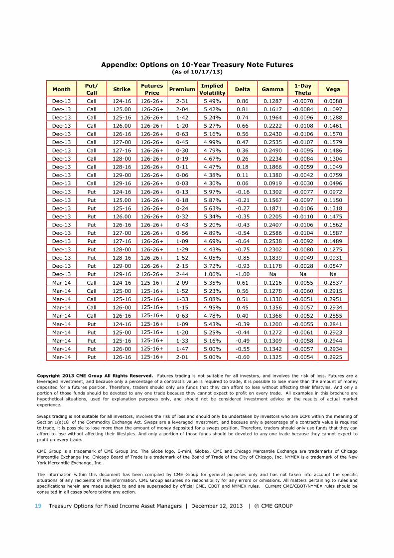
19 Treasury Options for Fixed Income Asset Managers | December 12, 2013 | © CME GROUP
Appendix: Options on 10-Year Treasury Note Futures (As of 10/17/13)
Month Put/
Call Strike
Futures
Price Premium
Implied
Volatility Delta Gamma
1-Day
Theta Vega
Dec-13 Call 124-16 126-26+ 2-31 5.49% 0.86 0.1287 -0.0070 0.0088
Dec-13 Call 125.00 126-26+ 2-04 5.42% 0.81 0.1617 -0.0084 0.1097
Dec-13 Call 125-16 126-26+ 1-42 5.24% 0.74 0.1964 -0.0096 0.1288
Dec-13 Call 126.00 126-26+ 1-20 5.27% 0.66 0.2222 -0.0108 0.1461
Dec-13 Call 126-16 126-26+ 0-63 5.16% 0.56 0.2430 -0.0106 0.1570
Dec-13 Call 127-00 126-26+ 0-45 4.99% 0.47 0.2535 -0.0107 0.1579
Dec-13 Call 127-16 126-26+ 0-30 4.79% 0.36 0.2490 -0.0095 0.1486
Dec-13 Call 128-00 126-26+ 0-19 4.67% 0.26 0.2234 -0.0084 0.1304
Dec-13 Call 128-16 126-26+ 0-11 4.47% 0.18 0.1866 -0.0059 0.1049
Dec-13 Call 129-00 126-26+ 0-06 4.38% 0.11 0.1380 -0.0042 0.0759
Dec-13 Call 129-16 126-26+ 0-03 4.30% 0.06 0.0919 -0.0030 0.0496
Dec-13 Put 124-16 126-26+ 0-13 5.97% -0.16 0.1302 -0.0077 0.0972
Dec-13 Put 125.00 126-26+ 0-18 5.87% -0.21 0.1567 -0.0097 0.1150
Dec-13 Put 125-16 126-26+ 0-24 5.63% -0.27 0.1871 -0.0106 0.1318
Dec-13 Put 126.00 126-26+ 0-32 5.34% -0.35 0.2205 -0.0110 0.1475
Dec-13 Put 126-16 126-26+ 0-43 5.20% -0.43 0.2407 -0.0106 0.1562
Dec-13 Put 127-00 126-26+ 0-56 4.89% -0.54 0.2586 -0.0104 0.1587
Dec-13 Put 127-16 126-26+ 1-09 4.69% -0.64 0.2538 -0.0092 0.1489
Dec-13 Put 128-00 126-26+ 1-29 4.43% -0.75 0.2302 -0.0080 0.1275
Dec-13 Put 128-16 126-26+ 1-52 4.05% -0.85 0.1839 -0.0049 0.0931
Dec-13 Put 129-00 126-26+ 2-15 3.72% -0.93 0.1178 -0.0028 0.0547
Dec-13 Put 129-16 126-26+ 2-44 1.06% -1.00 Na Na Na
Mar-14 Call 124-16 125-16+ 2-09 5.35% 0.61 0.1216 -0.0055 0.2837
Mar-14 Call 125-00 125-16+ 1-52 5.23% 0.56 0.1278 -0.0060 0.2915
Mar-14 Call 125-16 125-16+ 1-33 5.08% 0.51 0.1330 -0.0051 0.2951
Mar-14 Call 126-00 125-16+ 1-15 4.95% 0.45 0.1356 -0.0057 0.2934
Mar-14 Call 126-16 125-16+ 0-63 4.78% 0.40 0.1368 -0.0052 0.2855
Mar-14 Put 124-16 125-16+ 1-09 5.43% -0.39 0.1200 -0.0055 0.2841
Mar-14 Put 125-00 125-16+ 1-20 5.25% -0.44 0.1272 -0.0061 0.2923
Mar-14 Put 125-16 125-16+ 1-33 5.16% -0.49 0.1309 -0.0058 0.2944
Mar-14 Put 126-00 125-16+ 1-47 5.00% -0.55 0.1342 -0.0057 0.2934
Mar-14 Put 126-16 125-16+ 2-01 5.00% -0.60 0.1325 -0.0054 0.2925
Copyright 2013 CME Group All Rights Reserved. Futures trading is not suitable for all investors, and involves the risk of loss. Futures are a
leveraged investment, and because only a percentage of a contract’s value is required to trade, it is possible to lose more than the amount of money
deposited for a futures position. Therefore, traders should only use funds that they can afford to lose without affecting their lifestyles. And only a
portion of those funds should be devoted to any one trade because they cannot expect to profit on every trade. All examples in this brochure are
hypothetical situations, used for explanation purposes only, and should not be considered investment advice or the results of actual market
experience.
Swaps trading is not suitable for all investors, involves the risk of loss and should only be undertaken by investors who are ECPs within the meaning of
Section 1(a)18 of the Commodity Exchange Act. Swaps are a leveraged investment, and because only a percentage of a contract’s value is required
to trade, it is possible to lose more than the amount of money deposited for a swaps position. Therefore, traders should only use funds that they can
afford to lose without affecting their lifestyles. And only a portion of those funds should be devoted to any one trade because they cannot expect to
profit on every trade.
CME Group is a trademark of CME Group Inc. The Globe logo, E-mini, Globex, CME and Chicago Mercantile Exchange are trademarks of Chicago
Mercantile Exchange Inc. Chicago Board of Trade is a trademark of the Board of Trade of the City of Chicago, Inc. NYMEX is a trademark of the New
York Mercantile Exchange, Inc.
The information within this document has been compiled by CME Group for general purposes only and has not taken into account the specific
situations of any recipients of the information. CME Group assumes no responsibility for any errors or omissions. All matters pertaining to rules and
specifications herein are made subject to and are superseded by official CME, CBOT and NYMEX rules. Current CME/CBOT/NYMEX rules should be
consulted in all cases before taking any action.