"Transportation Network for Williams Technologies, Inc."

By: Erik Wikstrom and Jeff Cate

CSE 4395: SENIOR DESIGN

Instructor: Dr. Richard S. Barr

Date: May 9, 1996

I

II

TABLE OF CONTENTS

1. Project Summary 1.1. Description of the Problem 1.2. Method of Analysis 1.3. Results of the Analysis

2. Problem Background and Description 2.1. Problem Recognition 2.2. Problem Status 2.3. Project Objectives

3. Analysis of the Situation I 3.1. Modeling Considerations 3.2. Assumptions Made 3.3. Cost Determination I 3.4. Model Description 3.5. Illustrative Example of the Model

1 4. Technical Description of the Model 4.1. Cost Calculations 4.1.1. Distance Computations I 4.1.2. Determination of Air and Trucking Costs 4.1.3. Determination ofMode of Shipment and Route Unit Cost 4.1.4. Determination of Fired and Variable Cost of DC

I 4.2. Model Description 4.2.1. Model Formulation I 4.2.2. Design of the Network model 4.2.3. GAMS I/O andExecution

5. Analysis and Managerial Interpretation

6 Conclusions and Critique

Thanks

APPENDICES

1. PROJECT SUJvIIvIARY

This section includes an overview of the transportation project we completed for Williams

Technologies Incorporated. It provides brief descriptions of the problem, method of

analysis, and results of the analysis.

1.1. Description of the Problem

Williams Technologies Incorporated (WTI), intends to increase customer satisfaction by

decreasing time-to-market of its products, namely re-manufactured transmissions. WTI

believes this goal can be accomplished by developing a more efficient shipping system,

while minimizing the cost-to-market. This new system may be developed in-house or out-

sourced. Therefore, WTI needs an in-house solution that can be compared to those

submitted by outside sources.

1.2. Method of Analysis

A transportation model that includes all primary markets, secondary markets, distribution

centers, the production plant, and all combinations of connecting routes provides the basic

tool used in the analysis. The demands and costs used in the construction of the model are

based on projections from the prior year. More constraints and/or assumptions may be

added as needed to fine tune the model. This model provides the shipping route and

distribution center combination that yields the lowest total cost, while achieving WTI's

objective. The model can be modified to reflect changes in market demands, warehouse

costs, and shipping costs.

1.3. Results of the Analysis

The model indicates that a single distribution center that serves all markets should be

located in Charlotte, NC. This is a surprising result, which reflects the high fixed cost

I I 1 I E I I I I I I I I I I I I II

associated with establishing a distribution center. The fixed cost were determined through

a subjective method, which might not accurately reflect actual fixed cost. If better

information about fixed cost is entered into the model, the outcome might be substantially

different.

2. PROBLEM BACKGROUND AND DESCRIPTION

I I I I iI This section includes a further development of the problem. It provides a description of

the problem recognition, problem status, and the project objectives.

I2.1. Problem Recognition

IThe present shipping system at WTI, a re-manufacturer of automobile transmissions,

routes transmissions from WTI to the automobile manufacturers, which ship the

transmissions to the automobile dealerships. WTI recognizes an opportunity to decrease

product-to-market time by shipping its products directly to the automobile dealerships. An

efficient shipping system also represents an opportunity to lower consumer prices based

on a reduction of shipping cost.

2.2. Problem Status

WTI is accepting bids on a project that meets certain time-to-market requirements it has

made available to interested parties. WTI has also provided these parties with product

demand, weight, size, package, and other information relevant to the project. The bidding

parties use this information to develop solutions that will fulfill WTI's needs, while

enabling the bidding parties to make a profit on the service. In an effort to reach an

optimal solution, WTI has elected to develop their own model in conjunction with our

team from Southern Methodist University.

I I

I I I I I I I 1

I

I 1 2.3. Project Objectives

I The main objective is to provide maximum customer service while minimizing cost. In

I doing this, the model answers several logistic and cost questions. It decides in which cities

to locate distribution centers. It establishes which distribution center(s) serve each market.

The distance between the distribution center and market pairs determines shipment by air

or truck. The model determines the cost of all active routes, distribution centers, and

Ientire project. The model remains flexible, so changes can be made as conditions dictate.

I I F] I I I I I I I I I I

3. Analysis of the Situation.

In this section we will describe our general approach to the problem. This includes

discussion of: (1) modeling considerations, (2) assumptions, (3) cost determination, (4)

model description, and (5) an illustrative example.

3.1. Modeling Considerations.

After completing initial discussions with WTI, we felt that what needed to be determined

was the optimal number of distribution centers, where they should be positioned, and what

markets would be served by each distribution center. The way that we chose to solve this

problem was to model it using a mixed integer network. Because of the problem's

network characteristics, solution is more easily obtained than from other modeling

techniques. Binary variables were necessary in order to account for the fixed costs of

setting up distribution centers, while regular network flow arcs were used to account for

the flow of transmissions and the transportation costs incurred.

The first thing that we did in modeling the problem was to number all of the markets that

are served by WTI. This was done by sorting the markets alphabetically and then

assigning each market its own number in order. This was done to reduce the amount of

data entry and to aid in spreadsheet manipulation. The markets were divided by WTI into

54 primary markets and 153 secondary markets. Primary markets represent markets with

a large demand, and must be served within one day of a request for product. Secondary

markets represent markets with smaller demand and must be served within two days of a

request for product.

3.2. Assumptions Made

Some assumptions were made as to what markets were to be considered for distribution

center sites. First, all secondary markets were eliminated because of the very small

demand at each market and the relaxed time constraint of these cities. The next step was

to eliminate some of the primary markets as candidates to reduce the number of variables

in the problem. In the case that there were primary markets within 20 miles of each other,

one of the markets was chosen at random to represent that position. If a market of this

type was to make it into the optimal solution, the market with the smallest cost (real

estate, utilities, etc.) of the two would be chosen. The smallest of the primary markets

were eliminated due to the need for access to a major airport for facilitating air transport.

After these assumptions, the set of candidates for distribution center locatiot* was reduced

to 28 sites.

3.3. Cost Determination

Once we determined the set of candidates, our next step was to ascertain the costs

involved in the proposed distribution system. Transportation costs for the transmissions

are a function of distance, mode of transport and weight, so these data were needed.

Market demands were provided by WTI, based on projections from historical data.

Because of the extremely large number of possible routes(28*2075 796), we decided on

using straight line distance rather than road miles. These distances were calculated by

obtaining the latitude and longitude of each city, then using geometry to determine

distance (see calculations in next section.) Whether a city was to be served by truck or air

freight was computed by using its distance from the distribution center and whether it

required one-day service or two (see calc.) The cost of transportation over each route

was derived from the cost of shipping one unit one mile and then multiplying by the length

of the route (see calc.)

The cost of shipping transmissions from the plant in Charleston, SC to each of the

distribution centers was calculated in the same manner as the other route costs. An

assumption was made that the demand in Charleston would be supplied directly from the

plant. For this reason Charleston's demand was set to zero in the model, effectively

eliminating this demand from consideration.

Fixed and variable costs of placing a distribution center in a candidate market were

difficult to obtain because of the lack of historical data. These costs were ascertained by

I I I I 1• I I I I I I I I 1 I 1 I II

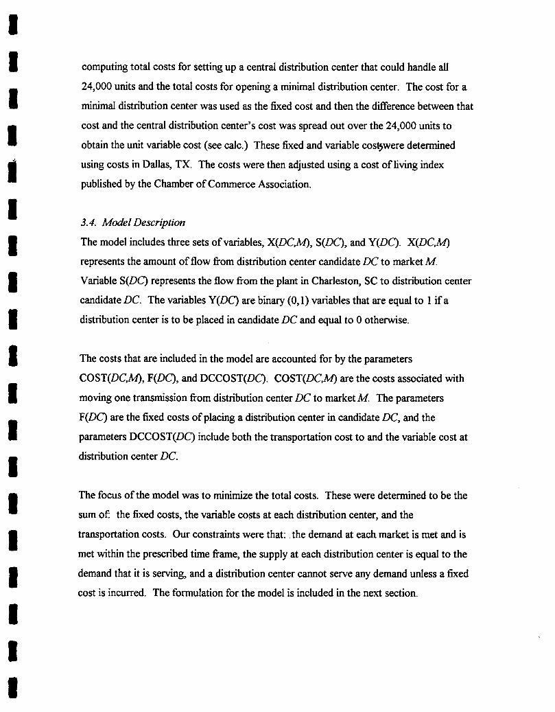
computing total costs for setting up a central distribution center that could handle all

24,000 units and the total costs for opening a minimal distribution center. The cost for a

minimal distribution center was used as the fixed cost and then the difference between that

cost and the central distribution center's cost was spread out over the 24,000 units to

obtain the unit variable cost (see caic.) These fixed and variable costwere determined

using costs in Dallas, TX. The costs were then adjusted using a cost of living index

published by the Chamber of Commerce Association.

3.4. Model Description

The model includes three sets of variables, X(DC,M), S(DC), and Y(DC). X(DC,M)

represents the amount of flow from distribution center candidate DC to market M

Variable S(DC) represents the flow from the plant in Charleston, SC to distribution center

candidate DC. The variables Y(DC) are binary (0,1) variables that are equal to 1 if a

distribution center is to be placed in candidate DC and equal to 0 otherwise.

The costs that are included in the model are accounted for by the parameters

COST(DC,M), F(DC), and DCCOST(DC). COST(DC,M) are the costs associated with

moving one transmission from distribution center DC to market M. The parameters

F(DC) are the fixed costs of placing a distribution center in candidate DC, and the

parameters DCCOST(DC) include both the transportation cost to and the variable cost at

distribution center DC.

The focus of the model was to minimize the total costs. These were determined to be the

sum of the fixed costs, the variable costs at each distribution center, and the

transportation costs. Our constraints were that: the demand at each market is met and is

met within the prescribed time frame, the supply at each distribution center is equal to the

demand that it is serving, and a distribution center cannot serve any demand unless a fixed

cost is incurred. The formulation for the model is included in the next section.

I I I Li I I I I I I I I I I I 1I I 1

\Iarkets

Demand

Demand

Demand

DC's

3.5. I/histraii'e Lxanipie ?f the Model

Following is an example of a comparable model on a smaller scale:

NETWORK FLOW DIAGRAM

Supply

In this example there are two possible distribution center sites serving three markets. The

fixed cost of establishing a distribution center at each location is $1,000. The costs

associated with transportation and the demands of each of the markets are included in the

following tables:

Table 3.5. a Transportation Costs Per Unit

DC's 1 2

LA $ 4.50 $ 9.00 Markets B $ 7.50 $ 4.00

Lic $ 9.50 $ 2.50

Table 3.5.b Demand

Market Demand A 50 B 30 C 60

I I I I 1 I 1 I I I I I I I I I 1 I 1

I I I I 1 I I I I I I I I I I I 1 I I

When this model is solved, the optimal solution establishes only one distribution center at

site two, which serves all three markets. The solution network is shown below:

NETWORK FLOW DIAGRAM

Markets DC's

No Flow l)emand - - - -

:

I)crnand •

Supply

I )cmandDC established

4. Technical Description otihe Model

This section includes the technical information regarding the model formulation and

calculations that we made. This information is divided into: (I) a breakdown of cost

calculations, and (2) a model description.

4. 1. Cost Calculations

4. 1. 1. i)is'1ance Computations

To calculate the large number of route distances, we went online to find the latitude and

longitude of each market city. These figures were available at

hup: www.mit.edu:8001geo. We placed the latitude and longitude figures into a

1 I Microsoft Excel spreadsheet and derived the following geometric formulae to convert

them .tof artesian coordinates:

X = cos(Lat)*cos(Long)

Y = sin(Lat)

Z = cos(Lat)*sin(Long)

From the Cartesian coordinates the straight-line distances between the cities were

computed by the distance formula:

d = ((X2-X1)2+(Y2-Y1)2+(Z2-Z1)2)'

Once this distance was obtained it was converted to the distance along the surface of the

earth by the conversion shown below:

Mean Earth Radius = 3958.832412

D = 2 * tan'(d/2t(1 - ( d/2))') * 3958.832412

These distances were verified by checking the computed values against values obtained

from an air mileage table for several of the routes. The computed values were within 2-3

miles of the tabulated values, which confirms our confidence in the use of these numbers.

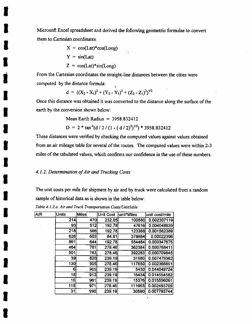
4.1.2. Determination of Air and Trucking Costs

The unit costs per mile for shipment by air and by truck were calculated from a random

sample of historical data as is shown in the table below:

Table 4.1.2. a Air and Truck Transportation Costs/Unit/Mile

lAIR Units Miles Unit Cost unit*Miles unit cost/mile

Li

214 470 232.05 100580 0.002307119 93 512 192.78 47616 0.004048639

218 566 192.78 123388 0.001562389 628 603 84.81 378684 0.00022396 861 644 192.78 554484 0.000347675 464 781 278.46 362384 0.000768411 501 783 278.46 392283 0.000709845

39 1 820 239.19 31980 0.007479362 130 905 278.46 117650 0.002366851

6 905 239.19 5430 0.044049724 18 913 239.19 16434 0.014554582 16 961 239.19 1 153761 0.015556061

115 971 278.461 1116651 0.002493709 311 990 239.191 306901 0.007793744

I

I

________

14 998 239.19 13972 0.017119238 11 1085 239.19 11935 0.020041056 25 1086 239.19 27150 0.008809945 14 1099 239.19 15386 0.015545951 17 1125 239.19 19125 0.012506667 21 1163 239.19 24423 0.009793637 AVG Cost/unit/mile 78 1289 239.19 100542 0.002379006 0.009069408

TRUCK Units Miles Unit Cost unit*Miles unit cost/mile 19 77 76.53 1463 0.052310321 33 111 77.87 3663 0.021258531 47 115 78.18 5405 0.014464385 70 120 76.2 8400 0.009071429

154 145 78.53 22330 0.003516794 9 166 76.88 1494 0.05145917

52 176 79.89 9152 0.00872924 65 194 78.18 12610 0.006199841 46 200 77.87 9200 0.00846413 10 201 79.89 2010 0.039746269 52 211 74.55 10972 0.006794568 47 230 79.22 10810 0.0073284 17 232 85.64 3944 0.021713996

100 237 .75.54 23700 0.003187342 154 2431 192.78 37422 0.005151515 29 243 74.55 7047 0.01 057897 39 254 85.34 9906 0.008614981 18 256 78.12 4608 0.016953125 51 278 74.55 14178 0.005258146 16 635 207.06 10160 0.020379921

5 664 70.43 3320 0.021213855 197 691 207.06 136127 0.001 521 08 AVG Cost/unit/mile

4 697 207.06 2788 0.074268293 0.018181926

I I I i I I I I I I I

4.1.3. Determination ofMode of Shipment and Route Unit Cost

IPer the requirements of WTI, primary markets within 400 miles and secondary markets

within 750 miles of a distribution center are to be serviced by truck. All markets beyond

Ithese respective ranges are to be serviced by air. These requirements ensure that market

demand is met within an acceptable time frame. We used a nested IF statement to

Ievaluate whether a market was primary or secondary and then to assign the proper mode

of shipment based upon the route distance. The route distance was then multiplied by the

1 appropriate unit cost/mile to determine the route cost per unit. A section of the Excel

spreadsheet is included. I Lj

HI 1

I -

Table 4.1.3. a Mode Shipment Determination and Route Unit Cost

Origin City St Market # Dest. City St distance Day Requirement Truck Air Route_Unit Cost Albany NY 1 Abilene TX 1572.9 2 0 1 28.59846085 Albany NY 2 Albany NY 0 1 1 0 0 Albany NY 3 Albany GA 954.8496 2 0 1 17.361 0758 Albany NY 4 Albuquerque NM 1 1832.527 1 0 1 1 33.3190001 Albany NY 5 Alexandria LA 1290.645 2 0 1 23.46650081 Albany NY 6Alpena Ml 509.0317 2 1 0 4.616408647 Albany NY 7 Amarillo TX 1584;847 2 0 1 28.61569607 Albany NY 8 Anchorage AK 3265.891 21 01 1 59.38041797 Albany INY I 9 Ardmore JOK 1388.9951 21 01 1 25.25470033

4.1.4. Determination of Fixed and Variable Cost of DC

Table 4.1.4. a Fixed and Variable Costs of DC

COST/SQ FT 3 COST PERSON 25000

Fixed Costs QTY COST OFFICE SPACE 1000 3000 WAREHOUSE SPACE 5000 15000 PERSONNEL 5 125000 INSURANCE 12 mos. 6000 EQUIPT (forklift, computers, etc.) 12 mos. 15000 UTILITIES 12 mos. 6000

170000

MAXIMUM WAREHOUSE INFO OFFICE SPACE 5000 15000 WAREHOUSE SPACE 20000 60000 PERSONNEL 15 375000 INSURANCE 12 mos. 27500 EQUIPT (forklift, computers, etc.) 12. mos. 30000 UTILITIES 1 12 mos. 12000

519500

Variable Costs OFFICE SPACE 0.17 0.51 WAREHOUSE SPACE 0.625 1.875 PERSONNEL 0.00042 10.5 INSURANCE 12 mos. 0.899 EQUIPT (forklift, computers, etc.) 12 mos. 0.625 UTILITIES 1 12 mos. 0.25

14.659

Ii1

4.2. Model Description

4.2.1. Model Formulation

The model formulation is as follows:

Parameters

COST(DC,M) : cost of transporting one unit from distribution center DC to

market m

DCCOST(DC) : unit cost at distribution center. DC including transportation

to distribution center DC

D(M) : demand at market M

F(DC) : fixed cost of placing a distribution center at site DC

TD = 24007 : total demand

Variables

X(DC,M) : flow from distribution center DC to market M

S(DC) : flow from plant in Charleston to distribution center DC

Binary Variables

Y(DC) : 0,1 variable; 1 if a distribution center is placed at site DC

Equations

minimize SUM((DC,M),COST(DC,M)*X(DC,M)) + SUM(DC,DCCOST(DC)*S(DC))

+ SUM(DC,F(DC)*Y(DC) [objective function]

subject to

SUM(DC,X(DC,M)) = D(M) for all M [demand constraint]

S(DC) = SUM(M,X(DC,M)) for all DC [supply constraint]

S(DC) <= TD*Y(DC) for all DC [fixed costs turned on/off]

X(DC,M), S(DC) >= 0 for DC, M [non-negativity]

I 1, 4.2.2 Design of the Network Model

The problem can be represented by a mixed integer network, with 5,824 flow arcs, 28 binary (1,0) arcs, and 236 nodes. See appendix B for illustration of the network.

4.2.3 GAMS I/O and Execution

The model that is described above was loaded onto titan. cis. smu.edu and run using GAMS, a high level language for formulating models with algebraic statements. GAMS is an interface for a variety of algorithmic solvers. For this mixed integer program, GAMS used CPLEX to solve for an optimal solution. The input files and GAMS formulation can be found in appendix C.

5. Analysis and Managerial. Interpretation.

The model's solution indicates that a. single distribution center should be established in. Charlotte, North Carolina. This distribution center will serve all markets in the model. Output from GAMS shows all flow, going from the plant.to.a distribution. center. in... Charlotte, and from there out to all markets. The only binary variable with a value of one is Y(36), the fixed cost variable associated with Charlotte. Refer to Appendix D for GAMS output.

6. Conclusions and Critique

After close examination of the results of the model output, we feel that the fixed cost data

Ithat was used might not accurately reflect true costs. While most of the other data that was used could be verified, our fixed cost data was quite subjective. Another possible source for error in the model is that transportation cost from the plant to the distribution I centers did not account for the fact that bulk shipments would have a lower unit transportation cost. We feel that if more accurate data were available, an alternate

I'

solution would probably be found to be optimal. We therefore recommend that management pursue accurate, verifiable cost data. This data could easily be entered into the model and the model resolved.

We would like to thank the following people for their help throughout the duration of this project: Dr. Richard S. Barr, Southern Methodist University Chris Emery, Director of Marketing, Williams Technologies, INC. Mike Champion, Return Products Management' David Welch, Systems Support; Southern Methodist University Mike McWhorter, Bolanz & Miller Realtors, INC. John Fargo, Lone Star Fork Lift

i

I I I I

I

I APPENDICES

I I I

I

I I I

I. I I I I

APPENDIX A: Coordinate Conversion Data 1 I,

I

Erik Wikstrom

From: Erik Scott Wikstrom Sent: Friday, May 03, 1996 4:59 AM To: Erik Wikstrom Subject: Lat-longs (fwd)

x = (mean radius of the earth) (longitude in radians) y = (mean radius of the earth)(latitude in radians) MEAN _EARTH _RADIUS = 6370949.0 1* Mean earth radius meters *1

MI—TM(m) ((m) * 1609.3) 1* statute miles to meters

1*_____________________________________________________________________

CONVERSIONS _--- ----------- - ---- _-_-- ---- --- *1

I

ANGULAR CONSTANTS AND

#define P1 3.14159265358979323846 #define TWOPI 6.2831 853071 7958647692 #define FOURPI 12.56637061435917295384 #deflne PIOVER2 1.57079632679489661923 #define PIOVER4 0.78539816339744830962

1*----------------------------------------------------- --------------------

LINEAR DISTANCE CONSTANTS AND CONVERSIONS

MI -- STATUTE MILES NMI - NAUTICAL MILES M - METERS FT - FEET KM -- KILOMETERS

------------------------

#define MI_TO_NMI(m) ((m) * 0 . 8683973)/* statute miles to nautical miles *1

#define N91—T-0—MI(n) ((n) * 1 . 1515466)/* nautical miles to statute miles */

#define FT_TO_M(f) ((f) * 0.304800) /* feet to meters *1

#define M_TO_FT(m) ((m) * 3 .280839) /* meters to feet */

#define MI_TO_KM(m) ((m) * 1.6093) /* statute miles to kilomters *1

#define MI—TM(m) ((m) * 1609.3) /* statute miles to meters */

#define KM—TO—MI(k) ((k) * 0.6214) /* kilomters to status miles */ #define M_TO_Ml(m) ((m) * 0.0006214) /* meters to nautical miles *1

#define NMI—TO—KM(n) ((n) * 1.853184) /* nautical miles to kilometers *1

#define NMI—TO—M(n) ((n) * 1853.184) /* nautical miles to meters *1

#define KM—TO—NMI(k) ((k) * 0.539622) /* kilometers to nautical miles *1

#define M_TO_NMI(m) ((m) * 0.000539622) /* meters to nautical miles

Page 1

HI

*1

I

I/* - - -- - ---- - ---------------

ANGULAR CONSTANTS AND CONVERSIONS ------------------------------------------------------------*1

#def,ne RAD_TO_DEG(r) ((r) * 57.29577951308232300) Pradians to degrees*/ #define DEG_TO_RAD(d) ((d) * 0.017453292519943295 ) Idegrees to radians*/

/* Degrees CW from north to deg. CCW from east *1 #define COMP—TO—GRAPH—DEG(d) (((d)<90.0) ? (-(d) + 90.0):(360.0 - (d) + 90.0))

/* Degrees CCW from east to deg. CW from north*/ #define GRAPHTOCOMPDEG(d) COMPTOGRAPHDEG(d)

/*___ ------ ---------- -------------------

PLANETARY CONSTANTS AND CONVERSIONS --------------------------- - --------------------- -------- -_--

#define POLAR—RADIUS 6356912.0 /* pole to pole distance meters *1 #define EARTH RADIUS 6371220.0 /* equatorial distance meters *1 #define MEAN_EARTH_RADIUS 6370949.0 /* Mean earth radius meters *1

1* Latitude degrees to arc seconds

#define DEG—TO—ARCS(I) ((I) * 3600)

Meters to latitude degrees *1 #define M_TO_LAT(m) ((m) * 360.0/(MEAN_EARTH_RADIUS*TWOPI))

r Latitude degrees to meters

*1 #define LAT_TO_M(I) ((I) * (MEAN_EARTH_RADIUS*TWOPI)/360.0)

1*Meters to longitude degrees at a given latitude

*1 #define M_TO_LNG(m,Iat) \ ((m) * (360.0/(MEAN_EARTH_RADIUS*cos(DEG_TO_RAD(Iat))1VV0pl)))

1* Longitude deg. to meters at a given latitude

*1 #define LNG_TO_M(lng,Iat) \ (((Ing) * MEAN_EARTH_RADI US*cos(DEG_TO_RAD(Iat))T\NOPI)/360.0)

1* Approximation for earth curvature

Page 2

Sheet9

Sample From Coordinate Conversion Spreadsheet Market # Dest. City ST LAT SEC LONG SEC DEC. LAT DEC. LON RAD LAT. RAD LOW X Y

I Abiline TX 32 36 0943 32.600 99.71667 0.568977 1.740384 -0.14219 0.538771 2 Albany NY 4239 - 7345 42.650 73.75 0.744383 1.28718 0.205816 0.677518 3 Albany GA 31 34 849 31.5'67 84.15 0.550942 1.468695 0.086843 0.52349 4 AlbuquerqNM 35 5 10639 35.083 106.65 0.61232 1.861394 -0.23447 0.574767 5 Alexandria LA 3118 0226 31.300 92.43333 0.546288 1.613266 -0.03628 0.519519 6 Alpena Ml 453 8325 45.050 83.41667 0.786271 1.455895 0.080998 0.707724 7 Amarillo TX 35 13 101 49 35.217 101.8167 0.614647 1.777036 -0.1673 0.57667 8 Anchorage AK 6113 14954 61.217 149.9 1.068432 2.616249 -0.41657 0.876447 9 Ardmore OK 34 10 978 34.167 97.13333 0.596321 1.695296 -0.10275 0.561602

10 Atlanta GA 3344 8423 33.733 84.38333 0.588758 1.472767 0.081394 0.555328 11 Augusta ME 44 18 6946 44.300 69.76667 0.773181 1.217658 0.247518 0.698415 12 Austin TX 30 16 9744 30.267 97.73333 0.528253 1.705768 -0.11622 0.504025 13 BakersfielcCA 3522 1191 35.367 119.0167 0.617265 2.077233 -0.39555 0.578807 14 Baltimore MD 39 17 7636 39.283 76.6 0.685624 1.336922 0.179379 0.633156 15 Bangor ME 44 48 68 46 44.800 68.76667 0.781908 1.200205 0.256983 0.704634 16 Baton Row LA 30 27 91 9 30.450 91.15 0.531453 1.590868 -0.0173 0.506786 17 Beaumont TX 30 5 94 6 30.083 94.1 0.525053 1.642355 -0.06187 0.501259 18 Bend OR 44 3 121 18 44.050 121.3 0.768818 2.117084 -0.3734 0.695286 19 Billings MT 45 47 108 30 45.783 108.5 0.79907 1.893682 -0.22128 0.716708

Page 1

- - - - - - -, - ,- - - - - - - - -

Sheet9

z 0.830367 0.706123 0.847594 0.784007 0.853688 0.701831 0.799664 0.241477 0.821 003 0.827639 0.671529 0.855834 0.71 3106 0.752952

0.6614 0.861898 0.863083 0.614128 0.661336

Page 2

- --IM - - - M, - ON - - - - - - - -

APPENDIX B: Network Diagram

NETWORK FLOW DIAGRAM Markets

DC's

Demand r—l),,

XDCM

1

Demand( 22

4^60

Charleston, SC

Demand (\,-)

3

Supply

DC : Place center at DC SDC : Supply to center DC XDCM : Flow from center DC to

market M

Demand( 4

Demand (20

- - - - - - - - - - - - - - - - - - -

APPENDIX C: GAMS Data

ISET M .Markets/i*207/

IDC(m) Distribution Centers /2, 10, 22, 26, 36, 40, 47, 51, 55, 57, 86, 99

$INCLUDE "demand.inc" INCLUDE "dccost.inc"

NINCLUDE "fixed.inc" INCLUDE cost.inctt

POSITIVE VARIABLES X(DC,M) Flow from DC dc to market m S(DC) Flow from Charleston to DC dc;

IVARIABLE Z Total cost;

BINARY VARIABLE Y(DC) 'lace a distribution center in DC dc;

I EQUATIONS TCOSt Total cost for project DEMAND(M) Demand for each market is met I DISTCON(DC) Supply at each distribution center FIX (DC) Fixed costs at each distribution center; I TCOST .. Z =E= StJM((DC,M),COST(DC,M)*X(DC,M)) + SUM(DC,F(DC)*Y(DC)) + SUM(DC,S(DC)*DCCOST(DC));

DEMAND(M) .. SUM(DC,X(DC,M)) =E= D(M); DISTCON(DC) S(DC) =E= SUM(M,X(DC,M)); FIX(DC) S(DC) =L= 1000000*Y(DC);

MODEL TRANSPORT A transportation network /ALL/; SOLVE TRANSPORT USING MIP MINIMIZING Z;

I I

'Parameters d(m) demand at market 1 16 2 140

4 112

7 25 8 73

10 384 11 24 12 130 13 16 14 106 15 23 16 I 32 17 18 18 4 19 I 20 11

16 21 14 22 154 23 I 6 24 13 25 42 I 26 844 27 4 28 18 29 17 I 30 132 31 68 32 9

I I 1 I I I

PARAMETERS /

COST (DC,M) Cost of shipping from dc DC to market m

I2 2

I2 2 2 I2 2

F - I I Ii

I

1 28.59846085 2 0 3 17.3610758 4 33.3190001 5 23.46650081 6 4.616408647 7 28.81569607 8 59.38041797 9 25.25470033 10 15.32816083 11 2.085274687 12 28.63822869 13 44.57731674 14 2.503408142 15 2.627481911 16 23.22348445 17 25.82577363 18 42.8638575 19 31.28481743 20 21.63540006 21 1.064068533 22 17.2306553 23 24.6588609 24 4.919751849 25 38.51282956 26 1.261407892 27 14.13636379 28 5.564454299 29 32.19673669 30 2.357924809 31 1.165425639 32 29.83596044 33 16.59936295 34 13.83664032 35 4.619484059 36 11.61448926 37 3.673608814 38 14.78378261 39 28.95191283 40 12.95021632 41 11.14677518 42 3.766451065 43 7.539510051 44 29.78431398 45 6.490119931 Mli

I I I I

Parameters dccost(dc) unit cost of throughput at dc as well as trans to dc

I/ 2 22.77848566

10 16.95804185 22 18.26103001

2624.7655862

36 16.22223752 40 22.845774 47 51

19.45057544 25.14771809

55 28.59272362

57

21.63275805 86 22.84521222 99 22.66225987 112 38.52991377

125

24.69901063 129 20.18298223 130 19.96948686 131 26.0079526

13617.32132465

142 21.14096315 143 31.11037199

14419.99541739

146 23.44270125 160 39.70245357

163 167

30.62585201 45.55771024

171 40.453325 181 20.79733797 197 18.88223526/;

I I I I I I I I I

Parameters f(dc) fixed cost of building a distribution center /2 199999.56

I10 161666.311 22 168166.2967 26 230999.4918

165332.9696 I

36 40 202666.2208 47 171166.2901

169999.626

I

51 55 177499.6095 57 191832.9113 86 208332.875

I. 99161832.9773

112 203499.5523 125 170499.6249

152332.9982

I

129 130 158166.3187 131 333332.6 136 163666.3066

I142 215999.5248 143 166332.9674 144 188832.9179

179832.9377 I

146 160 199999.56, 163 162499.6425

I

167 171

241166.1361 199499.5611

181 163666.3066 197 174999.615/;I

I I I I I I I I I

I I I I i I I I I APPENDIX D: GAMS Model. 1st Output

I I I I I I I I I I

MODEL STATISTICS

BLOCKS OF EQUATIONS 4 SINGLE EQUATIONS 264 BLOCKS OF VARIABLES 4 SINGLE VARIABLES 5853 NON ZERO ELEMENTS 17501 DISCRETE VARIABLES 28

Cplex 4.0, GAMS Link 8-6, DEC AXP/OSF Solution satisfies tolerances.

MEP Solution : 956498.369383 (6067 iterations, 158 nodes) Final LP : 956498.369383 (0 iterations)

Best integer solution possible: 934461.123924 Relative gap : 0.0235828

EQU FIX Fixed costs at each distribution center

LOWER LEVEL UPPER MARGINAL

2 -INF . . -8.651 10 -INF . -9.899 22 -INF . -11.218 26 -INF . . -7.226 36 -1NF -9.760E+5 40 -INF . . -10.408 47 -INF . . -8.810 51 -INF . . -13.054 55 -1NF . . -17.458 57 -INF . . -8.798 86 -INF . . -8446 99 -INF . . -14.825 112 -INF . . -16.739 125 -INF . . -14.172 129 -INF . . -8.188 130 -1NF . . -13.046 131 -INF . . -4.392 136 -INF . . -8.939 142 -INF . . -8.560 136 -INF . . -8.939 142 -INF . . -8.560 143 -INF . . -21.038 144 -INF . . -8.337 146 -INF . . -34.331 160 -INF . . -17.623 163 -INF . . -22.784

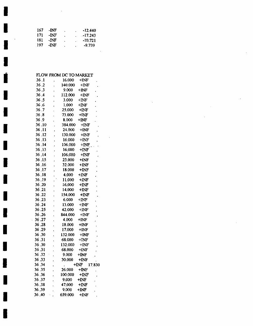
I 167 -INF . . -12.440 171 -INF . . -17.243 181 -INF . . -10.721 197 -INF . . -9.739

FLOW FROM DC TO MARKET 36.1 . 16.000 +INF 36.2 . 140.000 +INF 36.3 . 9.000 +INF 36.4 . 112.000 +INF 36.5 . 3.000 +INF 36.6 . 1.000 +INF 36.7 . 25.000 +INF 36.8 . 73.000 +INF 36.9 . 8.000 +INF 36.10 . 384.000 +ThF 36.11 . 24.000 +1NF 36.12 . 130.000 +INF 36.13 . 16.000 +INF 36.14 . 106.000 +1NF 36.13 . 16.000 +INF 36.14 . 106.000 +JNF 36.15 . 23.000 +INF 36.16 . 32.000 +INF 36.17 . 18.000 +INF 36.18 . 4.000 +ThW 36.19 . 11.000 +INF 36.20 . 16.000 +JNF 36.21 . 14.000 +ThF 36.22 . 154.000 +INF 36.23 . 6.000 +INF 36.24 . 13.000 +1NF 36 .25 . 42.000 +INF 36.26 . 844.000 +fr4F 36.27 . 4.000 +INF 36.28 . 18.000 +INF 36.29 . 17.000 +1NF 36.30 . 132.000 +INF 36.31 . 68.000 +INF 36.30 . 132.000 +INF 36.31 . 68.000 +INF 36.32 . 9.000 +INF 36 .33 . 30.000 +INF 36.34 . . +INF 17.830 36 .35 . 26.000 +INF 36 .36 . 100.000 +INF 36.37 . 9.000 +INF 36.38 . 47.000 +INF 36.39 . 9.000 +INF 36.40 . 659.000 +1NF

I I I I I I I I I I I I I I

I II

36.41 . 100.000 +1NF 36.42 . 7.000 +INF 36.43 . 270.000 +1NF 36.44 . 107.000 +INF 36 .45 . 52.000 +JNF 36.46 . 17.000 +INF 36.47 . 167.000 +INF 36.48 . 33.000 +JNF 36.47 . 167.000 +INF 36.48 . 33.000 +INF 36.49 . 16.000 +INF 36.50 . 31.000 +INF 36.51 . 464.000 +INF 36.52 . 12.000 +INF 36.53 . 29.000 +INF 36 .54 . 22.000 +llF 36 .55 . 644.000 +INF 36.56 . 22.000 +INF 36.57 . 174.000 +INF 36 .58 . 46.000 +INF 36 .59 . 8.000 +INF 36.60 . 18.000 +1NF 36.61 . 78.000 +INF 36.62 . 17.000 +JNF 36.63 . 18.000 +INF 36.64 . 88.000 +INF 36.65 . 12.000 +INF 36.66 . 7.000 +JNF 36.67 . 13.000 +INF 36.68 . 25.000 +INF 36.69 . 10.000 +INF 36.70 . 5.000 +U-4F 36.71 . 22.000 +INF 36.72 . 56.000 +INF 36.73 . 20.000 +flF 36.72 . 56.000 +INF 36.73 . 20.000 +1NF 36.74 . 10.000 +llF 36 .75 . 36.000 +INF 36.76 . 30.000 +JNF 36.77 . 52.000 +INF 36.78 . 8.000 +INF 36.79 . 23.000 +INF 36.80 . 66.000 +JNF 36.81 . 70.000 +INF 36.82 . 47.000 +INF 36.83 . 12.000 +INF 36.84 . 84.000 +INF 36.85 . 13.000 +INF 36.86 . 457.000 +INF 36.87 . 11.000 +INF 36.88 . 16.000 +INF 36.89 . 501.000 +INF 36.90 . 52.000 +1NF

I 36.89 . 501.000 +R-4F 36.90 . 52.000 +INF 36.91 . 27.000 +flF 36.92 . 91.000 +INF 36.93 . 6.000 +INF 36.94 . 50.000 +JNF 36 .95 . 197.000 +INF 36.96 . 76.000 +JNF 36 .97 . 2.000 +INF 36.98 . 17.000 +INF 36.99 . 147.000 +INIF 36.100 . 65.000 +INF 36.101 . 14.000 +INF 36 .102 . 38.000 +INF 36.103 . 2.000 +INF 36.104 . 21.000 +INF 36.105 . 16.000 +INF 36.106 . 14.000 +INF 36.107 . 83.000 +INF 36.106 . 14.000 +INF 36.107 . 83.000 +INF 36.108 . 63.000 +INF 36.109 . 2.000 +INF 36.110 . 26.000 +INF 36.111 . 26.000 +INP 36.112 . 1880.000 +INF 36.113 . 53.000 +INF 36.114 . 14.000 +INF 36.115 . 19.000 +fNF 36.116 . 41.000 +INF 36.117 : 5.000 +INF 36.118 . 5.000 +llF 36 .119 . 25.000 +INF 36.120 . 173.000 +INF 36 .121 . 5.000 +INF 36.122 . 861.000 +INF 36.123 . 21.000 +INF 36.124 . 95.000 +fNF 36.125 . 279.000 +JNF 36.126 . 14.000 +1NF 36.127 . 114.000 +INF 36 .128 . 10.000 +INF 36 .129 . 154.000 +INF 36.130 . 214.000 +INF 36.131 . 3387.000 +INF 36.132 . 65.000 +JNF 36.131 . 3387.000 +INF 36.132 . 65.000 +INF 36 .133 . . +INF 37.185 36.134 . 93.000 +INF 36 .135 . 62.000 +INF 36.136 . 249.000 +1NF 36.137 . 11.000 +INF 36.138 . 9.000 +INF

I I I I I I I I I I I U I I I I 1 I

I 36.139 . 17.000 +INF 36.140 . 4.000 +ll4F 36.141 . 11.000 +INF 36.142 . 1207.000 +INF 36.143 . 409.000 +1NF 36.144 . 200.000 +1NF 36.145 . 315.000 +INF 36.146 . 121.000 +INF 36.147 . 1.000 +INF 36.148 . 249.000 -I-INF 36.149 . . +INF 22.239 36.150 . 139.000 +INF 36.151 . 9.000 +INF 36.152 . 12.000 +INF 36.153 . 54.000 +INF 36.154 . 93.000 +JNF 36 .155 . 40.000 +INF 36 .156 . 89.000 +INF 36 .157 . 15.000 +INF 36 .158 . 8.000 +INF 36.159 . 4.000 +INF 36.160 . 174.000 +JNF 36.161 . 58.000 +1NF 36.162 . 2.000 +INF 36 .163 . 253.000 +JNF 36.164 . 11.000 +INF 36 .165 . 115.000 +INF 36.166 . 358.000 +INF 36.165 . 115.000 +INF 36.166 . 358.000 +INF 36.167 .' 652.000 +INF 36.168 . 28.000 +INF 36.169 . 29.000 +INF 36.170 . 53.000 +INP 36.171 . 624.000 +INF 36.172 . 47.000 +INF 36 .173 . 37.000 +1NF 36 .174 . 1.000 +INF 36 .173 . 37.000 +INF 36 .174 . 1.000 +1NF 36 .175 . 25.000 +INF 36.176 . 15.000 +INF 36.177 . 69.000 +INF 36.178 106.000 +INF 36 .179 . 28.000 +JNF 36 .180 . 3.000 +INF 36.181 . 103.000 +INF 36.182 . 118.000 +INF 36.183 . 39.000 +llF 36.184 . 389.000 +INF 36 .185 . 4.000 +INF 36.186 . 28.000 +INF 36 .187 . 13.000 +INF 36.188 . 2.000 +JNF

I I I I I I I I I I I 1 I I I I I I

I 36.189 . 93.000 +INF 36.190 . 54.000 +INF 36.191 . 10.000 +INF 36.190 . 54.000 +INF 36.191 . 10.000 +INF 36.192 . 23.000 +INF. 36.193 . 41.000 +1NF 36.194 . 25.000 +INF 36.195 . 6.000 -4-INF 36.196 . 39.000 +INF 36.197 . 628.000 +1NF 36.198 . 14.000 +INF 36.199 . 20.000 +1NF 36.200 . 218.000 +INF 36 .201 . 6.000 +JNF 36.202 . 29.000 +JNF 36.203 . 18.000 +INF 36.204 . 28.000 +1NF 36 .205 . 16.000 +flF 36.206 . 16.000 +1NF 36.207 . . +INF 19.234

I I I I I I I

Flow from plant to Distribution Center DC L. Level U. 2 . . +INF 10 . . +JNF 22 . . +INF 26 . . +INF 36 . 23956.000 +INF 40 . . +INF 47 . . +INF 51 . . +INF 55 . . +fls.IF 57 . . +INF 86 . . +JNF 99 . . +JNF 112 . . +INF 125 . . +INF 129 . . 130 . . +1NF 131 . . +INF 136 . . +INF 142 . . +1NF 143 . . +1F 144 . . +INF 146 . . +INF 160 . . +INF 163 . . +INF 167 . . +ThIF 171 . . +INF 181 . . +INF 197 . . +INF

I I I I I I I I I II