Transportation Complete
122
© 2008 Prentice-Hall, Inc. Chapter 10 To accompany Quantitative Analysis for Management, Tenth Edition, by Render, Stair, and Hanna Power Point slides created by Jeff Heyl Transportation and Assignment Models © 2009 Prentice-Hall, Inc.
-
Upload
abie-de-la-paz -
Category
Documents
-
view
77 -
download
0
Transcript of Transportation Complete

© 2008 Prentice-Hall, Inc.
Chapter 10
To accompanyQuantitative Analysis for Management, Tenth Edition, by Render, Stair, and Hanna Power Point slides created by Jeff Heyl
Transportation and Assignment Models
© 2009 Prentice-Hall, Inc.

© 2009 Prentice-Hall, Inc. 10 – 2
Learning Objectives
1. Structure special LP problems using the transportation and assignment models
2. Use the northwest corner, VAM, MODI, and stepping-stone methods
3. Solve facility location and other application problems with transportation models
4. Solve assignment problems with the Hungarian (matrix reduction) method
After completing this chapter, students will be able to:After completing this chapter, students will be able to:

© 2009 Prentice-Hall, Inc. 10 – 3
Chapter Outline
10.110.1 Introduction10.210.2 Setting Up a Transportation Problem10.310.3 Developing an Initial Solution: Northwest
Corner Rule10.410.4 Stepping-Stone Method: Finding a
Least-Cost Solution10.510.5 MODI Method10.610.6 Vogel’s Approximation Method: Another
Way to Find an Initial Solution10.710.7 Unbalanced Transportation Problems

© 2009 Prentice-Hall, Inc. 10 – 4
Chapter Outline
10.810.8 Degeneracy in Transportation Problems10.910.9 More Than One Optimal Solution10.1010.10 Maximization Transportation Problems10.1110.11 Unacceptable or Prohibited Routes10.1210.12 Facility Location Analysis10.1310.13 Assignment Model Approach10.1410.14 Unbalanced Assignment Problems10.1510.15 Maximization Assignment Problems
© 2009 Prentice-Hall, Inc. 10 – 5
Introduction
In this chapter we will explore two special linear programming models The transportation model The assignment model
Because of their structure, they can be solved more efficiently than the simplex method
These problems are members of a category of LP techniques called network flow network flow problemsproblems

© 2009 Prentice-Hall, Inc. 10 – 6
Introduction
Transportation model The transportation problemtransportation problem deals with the
distribution of goods from several points of supply (sourcessources) to a number of points of demand (destinationsdestinations)
Usually we are given the capacity of goods at each source and the requirements at each destination
Typically the objective is to minimize total transportation and production costs
© 2009 Prentice-Hall, Inc. 10 – 7
Introduction
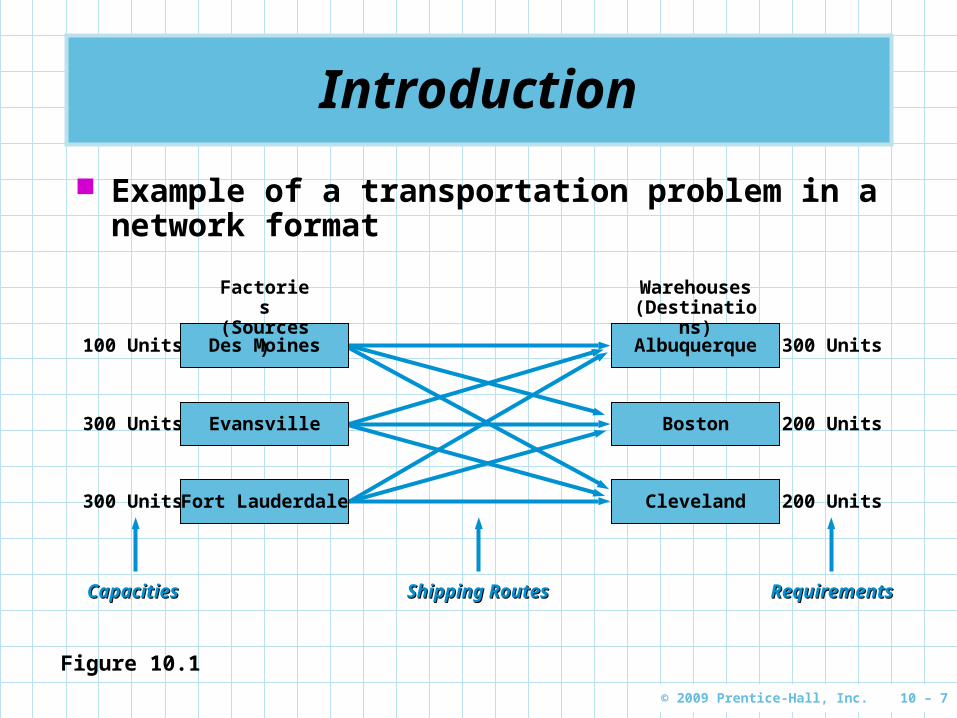
Example of a transportation problem in a network format
100 Units
300 Units
300 Units 200 Units
200 Units
300 Units
Factories (Sources)
Des Moines
Evansville
Fort Lauderdale
Warehouses (Destinations)
Albuquerque
Boston
Cleveland
CapacitiesCapacities Shipping RoutesShipping Routes RequirementsRequirements
Figure 10.1

© 2009 Prentice-Hall, Inc. 10 – 8
Introduction
Assignment model The assignment problemassignment problem refers to the class of
LP problems that involve determining the most efficient assignment of resources to tasks
The objective is most often to minimize total costs or total time to perform the tasks at hand
One important characteristic of assignment problems is that only one job or worker can be assigned to one machine or project

© 2009 Prentice-Hall, Inc. 10 – 9
Introduction
Special-purpose algorithms Although standard LP methods can be used to
solve transportation and assignment problems, special-purpose algorithms have been developed that are more efficient
They still involve finding and initial solution and developing improved solutions until an optimal solution is reached
They are fairly simple in terms of computation

© 2009 Prentice-Hall, Inc. 10 – 10
Introduction
Streamlined versions of the simplex method are important for two reasons
1. Their computation times are generally 100 times faster 2. They require less computer memory (and hence can
permit larger problems to be solved) Two common techniques for developing initial
solutions are the northwest corner method and Vogel’s approximation
The initial solution is evaluated using either the stepping-stone method or the modified distribution (MODI) method
We also introduce a solution procedure called the Hungarian methodHungarian method, Flood’s techniqueFlood’s technique, or the reduced matrix methodreduced matrix method

© 2009 Prentice-Hall, Inc. 10 – 11
Setting Up a Transportation Problem
The Executive Furniture Corporation manufactures office desks at three locations: Des Moines, Evansville, and Fort Lauderdale
The firm distributes the desks through regional warehouses located in Boston, Albuquerque, and Cleveland
Estimates of the monthly production capacity of each factory and the desks needed at each warehouse are shown in Figure 10.1

© 2009 Prentice-Hall, Inc. 10 – 12
Setting Up a Transportation Problem
Production costs are the same at the three factories so the only relevant costs are shipping from each sourcesource to each destinationdestination
Costs are constant no matter the quantity shipped
The transportation problem can be described as how to select the shipping routes to be used and how to select the shipping routes to be used and the number of desks to be shipped on each route the number of desks to be shipped on each route so as to minimize total transportation costso as to minimize total transportation cost
Restrictions regarding factory capacities and warehouse requirements must be observed

© 2009 Prentice-Hall, Inc. 10 – 13
Setting Up a Transportation Problem
The first step is setting up the transportation table
Its purpose is to summarize all the relevant data and keep track of algorithm computations
Transportation costs per desk for Executive Furniture
TOFROM ALBUQUERQUE BOSTON CLEVELAND
DES MOINES $5 $4 $3
EVANSVILLE $8 $4 $3
FORT LAUDERDALE $9 $7 $5
Table 10.1

© 2009 Prentice-Hall, Inc. 10 – 14
Setting Up a Transportation Problem
Geographical locations of Executive Furniture’s factories and warehouses
Albuquerque
Cleveland
Boston
Des Moines
Fort Lauderdale
Evanston
Factory
Warehouse
Figure 10.2
© 2009 Prentice-Hall, Inc. 10 – 15
Setting Up a Transportation Problem
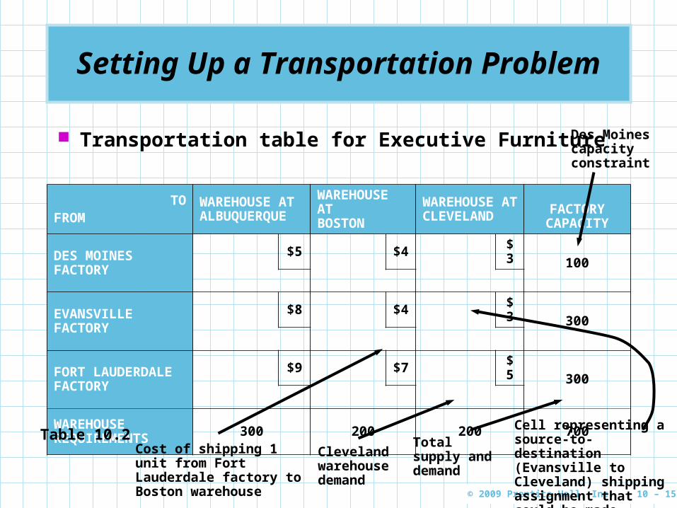
Transportation table for Executive Furniture
TOFROM
WAREHOUSE AT ALBUQUERQUE
WAREHOUSE AT BOSTON
WAREHOUSE AT CLEVELAND
FACTORY CAPACITY
DES MOINES FACTORY
$5 $4 $3100
EVANSVILLE FACTORY
$8 $4 $3300
FORT LAUDERDALE FACTORY
$9 $7 $5300
WAREHOUSE REQUIREMENTS 300 200 200 700
Table 10.2
Des Moines capacity constraint
Cell representing a source-to-destination (Evansville to Cleveland) shipping assignment that could be made
Total supply and demandCleveland
warehouse demand
Cost of shipping 1 unit from Fort Lauderdale factory to Boston warehouse

© 2009 Prentice-Hall, Inc. 10 – 16
Setting Up a Transportation Problem
In this table, total factory supply exactly equals total warehouse demand
When equal demand and supply occur, a balanced problembalanced problem is said to exist
This is uncommon in the real world and we have techniques to deal with unbalanced problems
© 2009 Prentice-Hall, Inc. 10 – 17
Developing an Initial Solution: Northwest Corner Rule
Once we have arranged the data in a table, we must establish an initial feasible solution
One systematic approach is known as the northwest corner rulenorthwest corner rule
Start in the upper left-hand cell and allocate units to shipping routes as follows
1. Exhaust the supply (factory capacity) of each row before moving down to the next row
2. Exhaust the demand (warehouse) requirements of each column before moving to the right to the next column
3. Check that all supply and demand requirements are met. In this problem it takes five steps to make the
initial shipping assignments

© 2009 Prentice-Hall, Inc. 10 – 18
Developing an Initial Solution: Northwest Corner Rule
1. Beginning in the upper left hand corner, we assign 100 units from Des Moines to Albuquerque. This exhaust the supply from Des Moines but leaves Albuquerque 200 desks short. We move to the second row in the same column.
TOFROM
ALBUQUERQUE (A)
BOSTON (B)
CLEVELAND (C)
FACTORY CAPACITY
DES MOINES (D) 100100
$5 $4 $3100
EVANSVILLE (E)
$8 $4 $3300
FORT LAUDERDALE (F)
$9 $7 $5300
WAREHOUSE REQUIREMENTS 300 200 200 700

© 2009 Prentice-Hall, Inc. 10 – 19
Developing an Initial Solution: Northwest Corner Rule
2. Assign 200 units from Evansville to Albuquerque. This meets Albuquerque’s demand. Evansville has 100 units remaining so we move to the right to the next column of the second row.
TOFROM
ALBUQUERQUE (A)
BOSTON (B)
CLEVELAND (C)
FACTORY CAPACITY
DES MOINES (D) 100
$5 $4 $3100
EVANSVILLE (E) 200200
$8 $4 $3300
FORT LAUDERDALE (F)
$9 $7 $5300
WAREHOUSE REQUIREMENTS 300 200 200 700
© 2009 Prentice-Hall, Inc. 10 – 20
Developing an Initial Solution: Northwest Corner Rule
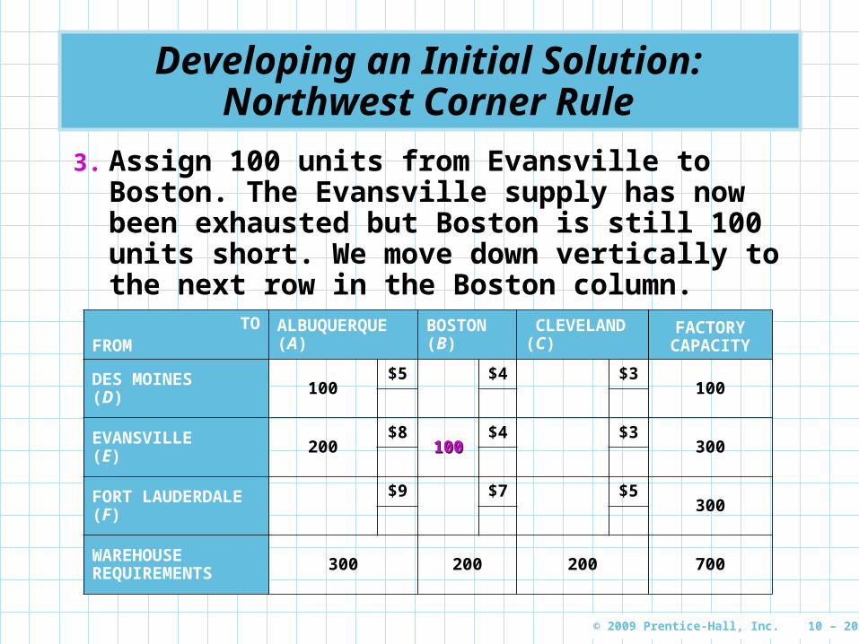
3. Assign 100 units from Evansville to Boston. The Evansville supply has now been exhausted but Boston is still 100 units short. We move down vertically to the next row in the Boston column.
TOFROM
ALBUQUERQUE (A)
BOSTON (B)
CLEVELAND (C)
FACTORY CAPACITY
DES MOINES (D) 100
$5 $4 $3100
EVANSVILLE (E) 200
$8100100
$4 $3300
FORT LAUDERDALE (F)
$9 $7 $5300
WAREHOUSE REQUIREMENTS 300 200 200 700
© 2009 Prentice-Hall, Inc. 10 – 21
Developing an Initial Solution: Northwest Corner Rule
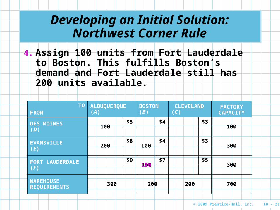
4. Assign 100 units from Fort Lauderdale to Boston. This fulfills Boston’s demand and Fort Lauderdale still has 200 units available.
TOFROM
ALBUQUERQUE (A)
BOSTON (B)
CLEVELAND (C)
FACTORY CAPACITY
DES MOINES (D) 100
$5 $4 $3100
EVANSVILLE (E) 200
$8100
$4 $3300
FORT LAUDERDALE (F)
$9100100
$7 $5300
WAREHOUSE REQUIREMENTS 300 200 200 700

© 2009 Prentice-Hall, Inc. 10 – 22
Developing an Initial Solution: Northwest Corner Rule
5. Assign 200 units from Fort Lauderdale to Cleveland. This exhausts Fort Lauderdale’s supply and Cleveland’s demand. The initial shipment schedule is now complete.
TOFROM
ALBUQUERQUE (A)
BOSTON (B)
CLEVELAND (C)
FACTORY CAPACITY
DES MOINES (D) 100
$5 $4 $3100
EVANSVILLE (E) 200
$8100
$4 $3300
FORT LAUDERDALE (F)
$9100
$7200200
$5300
WAREHOUSE REQUIREMENTS 300 200 200 700
Table 10.3
© 2009 Prentice-Hall, Inc. 10 – 23
Developing an Initial Solution: Northwest Corner Rule
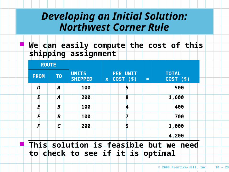
We can easily compute the cost of this shipping assignment
ROUTE
UNITS SHIPPED x
PER UNIT COST ($) =
TOTAL COST ($)FROM TO
D A 100 5 500
E A 200 8 1,600
E B 100 4 400
F B 100 7 700
F C 200 5 1,000
4,200
This solution is feasible but we need to check to see if it is optimal

© 2009 Prentice-Hall, Inc. 10 – 24
Stepping-Stone Method: Finding a Least Cost Solution
The stepping-stone methodstepping-stone method is an iterative technique for moving from an initial feasible solution to an optimal feasible solution
There are two distinct parts to the process Testing the current solution to determine if
improvement is possible Making changes to the current solution to
obtain an improved solution This process continues until the optimal
solution is reached

© 2009 Prentice-Hall, Inc. 10 – 25
Stepping-Stone Method: Finding a Least Cost Solution
There is one very important rule The number of occupied routes (or squares) must The number of occupied routes (or squares) must
always be equal to one less than the sum of the always be equal to one less than the sum of the number of rows plus the number of columnsnumber of rows plus the number of columns
In the Executive Furniture problem this means the initial solution must have 3 + 3 – 1 = 5 squares used
Occupied shipping routes (squares)
Number of rows
Number of columns= + – 1
When the number of occupied rows is less than this, the solution is called degeneratedegenerate
© 2009 Prentice-Hall, Inc. 10 – 26
Testing the Solution for Possible Improvement
The stepping-stone method works by testing each unused square in the transportation table to see what would happen to total shipping costs if one unit of the product were tentatively shipped on an unused route
There are five steps in the process

© 2009 Prentice-Hall, Inc. 10 – 27
Five Steps to Test Unused Squares with the Stepping-Stone Method
1. Select an unused square to evaluate2. Beginning at this square, trace a closed path
back to the original square via squares that are currently being used with only horizontal or vertical moves allowed
3. Beginning with a plus (+) sign at the unused square, place alternate minus (–) signs and plus signs on each corner square of the closed path just traced

© 2009 Prentice-Hall, Inc. 10 – 28
Five Steps to Test Unused Squares with the Stepping-Stone Method
4. Calculate an improvement indeximprovement index by adding together the unit cost figures found in each square containing a plus sign and then subtracting the unit costs in each square containing a minus sign
5. Repeat steps 1 to 4 until an improvement index has been calculated for all unused squares. If all indices computed are greater than or equal to zero, an optimal solution has been reached. If not, it is possible to improve the current solution and decrease total shipping costs.

© 2009 Prentice-Hall, Inc. 10 – 29
Five Steps to Test Unused Squares with the Stepping-Stone Method
For the Executive Furniture Corporation data
Steps 1 and 2Steps 1 and 2. Beginning with Des Moines–Boston route we trace a closed path using only currently occupied squares, alternately placing plus and minus signs in the corners of the path
In a closed pathclosed path, only squares currently used for shipping can be used in turning corners
Only oneOnly one closed route is possible for each square we wish to test

© 2009 Prentice-Hall, Inc. 10 – 30
Five Steps to Test Unused Squares with the Stepping-Stone Method
Step 3Step 3. We want to test the cost-effectiveness of the Des Moines–Boston shipping route so we pretend we are shipping one desk from Des Moines to Boston and put a plus in that box But if we ship one moremore unit out of Des Moines
we will be sending out 101 units Since the Des Moines factory capacity is only
100, we must ship fewerfewer desks from Des Moines to Albuquerque so we place a minus sign in that box
But that leaves Albuquerque one unit short so we must increase the shipment from Evansville to Albuquerque by one unit and so on until we complete the entire closed path

© 2009 Prentice-Hall, Inc. 10 – 31
Five Steps to Test Unused Squares with the Stepping-Stone Method
Evaluating the unused Des Moines–Boston shipping route
TOFROM
ALBUQUERQUE BOSTON CLEVELAND FACTORY CAPACITY
DES MOINES 100$5 $4 $3
100
EVANSVILLE 200$8
100$4 $3
300
FORT LAUDERDALE$9
100$7
200$5
300
WAREHOUSE REQUIREMENTS 300 200 200 700 Table 10.4
Warehouse B
$4Factory
D
Warehouse A
$5
100
FactoryE
$8
200
$4
100
+
– +
–

© 2009 Prentice-Hall, Inc. 10 – 32
Five Steps to Test Unused Squares with the Stepping-Stone Method
Evaluating the unused Des Moines–Boston shipping route
TOFROM
ALBUQUERQUE BOSTON CLEVELAND FACTORY CAPACITY
DES MOINES 100$5 $4 $3
100
EVANSVILLE 200$8
100$4 $3
300
FORT LAUDERDALE$9
100$7
200$5
300
WAREHOUSE REQUIREMENTS 300 200 200 700 Table 10.4
Warehouse A
FactoryD
$5
Warehouse B
$4
FactoryE
$8 $4
100
200 100
201
991
+
– +
–99

© 2009 Prentice-Hall, Inc. 10 – 33
Five Steps to Test Unused Squares with the Stepping-Stone Method
Evaluating the unused Des Moines–Boston shipping route
TOFROM
ALBUQUERQUE BOSTON CLEVELAND FACTORY CAPACITY
DES MOINES 100$5 $4 $3
100
EVANSVILLE 200$8
100$4 $3
300
FORT LAUDERDALE$9
100$7
200$5
300
WAREHOUSE REQUIREMENTS 300 200 200 700 Table 10.4
Warehouse A
FactoryD
$5
Warehouse B
$4
FactoryE
$8 $4
100
991
201
200 100
99+
– +
–
Result of Proposed Shift in Allocation
= 1 x $4– 1 x $5+ 1 x $8– 1 x $4 = +$3

© 2009 Prentice-Hall, Inc. 10 – 34
Five Steps to Test Unused Squares with the Stepping-Stone Method
Step 4Step 4. We can now compute an improvement indeximprovement index (IIijij) for the Des Moines–Boston route We add the costs in the squares with plus signs
and subtract the costs in the squares with minus signs
Des Moines–Boston index = IDB = +$4 – $5 + $5 – $4 = + $3
This means for every desk shipped via the Des Moines–Boston route, total transportation cost will increaseincrease by $3 over their current level

© 2009 Prentice-Hall, Inc. 10 – 35
Five Steps to Test Unused Squares with the Stepping-Stone Method
Step 5Step 5. We can now examine the Des Moines–Cleveland unused route which is slightly more difficult to draw
Again we can only turn corners at squares that represent existing routes
We must pass through the Evansville–Cleveland square but we can not turn there or put a + or – sign
The closed path we will use is+ DC – DA + EA – EB + FB – FC

© 2009 Prentice-Hall, Inc. 10 – 36
Five Steps to Test Unused Squares with the Stepping-Stone Method
Evaluating the Des Moines–Cleveland shipping route
TOFROM
ALBUQUERQUE BOSTON CLEVELAND FACTORY CAPACITY
DES MOINES 100$5 $4 $3
100
EVANSVILLE 200$8
100$4 $3
300
FORT LAUDERDALE$9
100$7
200$5
300
WAREHOUSE REQUIREMENTS 300 200 200 700
Table 10.5
Start
+
+ –
–
+ –
Des Moines–Cleveland improvement index = IDC = + $3 – $5 + $8 – $4 + $7 – $5 = + $4
© 2009 Prentice-Hall, Inc. 10 – 37
Five Steps to Test Unused Squares with the Stepping-Stone Method
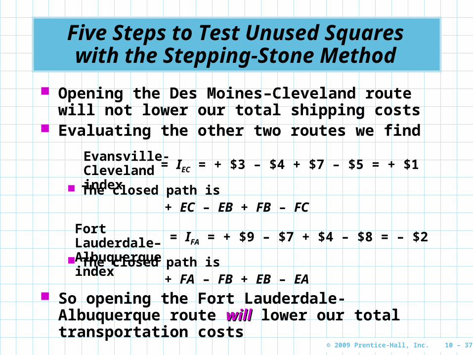
Opening the Des Moines–Cleveland route will not lower our total shipping costs
Evaluating the other two routes we find
The closed path is+ EC – EB + FB – FC
The closed path is+ FA – FB + EB – EA
So opening the Fort Lauderdale-Albuquerque route willwill lower our total transportation costs
Evansville-Cleveland index = IEC = + $3 – $4 + $7 – $5 = + $1
Fort Lauderdale–Albuquerque index = IFA = + $9 – $7 + $4 – $8 = – $2

© 2009 Prentice-Hall, Inc. 10 – 38
Obtaining an Improved Solution
In the Executive Furniture problem there is only one unused route with a negative index (Fort Lauderdale-Albuquerque)
If there was more than one route with a negative index, we would choose the one with the largest improvement
We now want to ship the maximum allowable number of units on the new route
The quantity to ship is found by referring to the closed path of plus and minus signs for the new route and selecting the smallest numbersmallest number found in those squares containing minus signs

© 2009 Prentice-Hall, Inc. 10 – 39
Obtaining an Improved Solution
To obtain a new solution, that number is added to all squares on the closed path with plus signs and subtracted from all squares the closed path with minus signs
All other squares are unchanged In this case, the maximum number that can be
shipped is 100 desks as this is the smallest value in a box with a negative sign (FB route)
We add 100 units to the FA and EB routes and subtract 100 from FB and EA routes
This leaves balanced rows and columns and an improved solution

© 2009 Prentice-Hall, Inc. 10 – 40
Obtaining an Improved Solution
Stepping-stone path used to evaluate route FA
TOFROM
A B C FACTORY CAPACITY
D 100$5 $4 $3
100
E 200$8
100$4 $3
300
F$9
100$7
200$5
300
WAREHOUSE REQUIREMENTS 300 200 200 700
Table 10.6
+
+ –
–

© 2009 Prentice-Hall, Inc. 10 – 41
Obtaining an Improved Solution
Second solution to the Executive Furniture problem
TOFROM
A B C FACTORY CAPACITY
D 100$5 $4 $3
100
E 100$8
200$4 $3
300
F 100$9 $7
200$5
300
WAREHOUSE REQUIREMENTS 300 200 200 700
Table 10.7
Total shipping costs have been reduced by (100 units) x ($2 saved per unit) and now equals $4,000

© 2009 Prentice-Hall, Inc. 10 – 42
Obtaining an Improved Solution
This second solution may or may not be optimal To determine whether further improvement is
possible, we return to the first five steps to test each square that is nownow unused
The four new improvement indices are
D to B = IDB = + $4 – $5 + $8 – $4 = + $3(closed path: + DB – DA + EA – EB)
D to C = IDC = + $3 – $5 + $9 – $5 = + $2(closed path: + DC – DA + FA – FC)
E to C = IEC = + $3 – $8 + $9 – $5 = – $1(closed path: + EC – EA + FA – FC)
F to B = IFB = + $7 – $4 + $8 – $9 = + $2(closed path: + FB – EB + EA – FA)

© 2009 Prentice-Hall, Inc. 10 – 43
Obtaining an Improved Solution
An improvement can be made by shipping the maximum allowable number of units from E to C
TOFROM
A B C FACTORY CAPACITY
D 100$5 $4 $3
100
E 100$8
200$4 $3
300
F 100$9 $7
200$5
300
WAREHOUSE REQUIREMENTS 300 200 200 700
Table 10.8
Path to evaluate for the EC route
Start
+
+ –
–

© 2009 Prentice-Hall, Inc. 10 – 44
Obtaining an Improved Solution
Total cost of third solution
ROUTE
DESKS SHIPPED x
PER UNIT COST ($) =
TOTAL COST ($)FROM TO
D A 100 5 500
E B 200 4 800
E C 100 3 300
F A 200 9 1,800
F C 100 5 500
3,900

© 2009 Prentice-Hall, Inc. 10 – 45
Obtaining an Improved Solution
TOFROM
A B C FACTORY CAPACITY
D 100$5 $4 $3
100
E$8
200$4
100$3
300
F 200$9 $7
100$5
300
WAREHOUSE REQUIREMENTS 300 200 200 700
Table 10.9
Third and optimal solution

© 2009 Prentice-Hall, Inc. 10 – 46
Obtaining an Improved Solution
This solution is optimal as the improvement indices that can be computed are all greater than or equal to zero
D to B = IDB = + $4 – $5 + $9 – $5 + $3 – $4 = + $2+ $2(closed path: + DB – DA + FA – FC + EC – EB)
D to C = IDC = + $3 – $5 + $9 – $5 = + $2+ $2(closed path: + DC – DA + FA – FC)
E to A = IEA = + $8 – $9 + $5 – $3 = + $1+ $1(closed path: + EA – FA + FC – EC)
F to B = IFB = + $7 – $5 + $3 – $4 = + $1 + $1(closed path: + FB – FC + EC – EB)

© 2009 Prentice-Hall, Inc. 10 – 47
Summary of Steps in Transportation Algorithm (Minimization)
1. Set up a balanced transportation table2. Develop initial solution using either the northwest
corner method or Vogel’s approximation method3. Calculate an improvement index for each empty
cell using either the stepping-stone method or the MODI method. If improvement indices are all nonnegative, stop as the optimal solution has been found. If any index is negative, continue to step 4.
4. Select the cell with the improvement index indicating the greatest decrease in cost. Fill this cell using the stepping-stone path and go to step 3.

© 2009 Prentice-Hall, Inc. 10 – 48
Using Excel QM to Solve Transportation Problems
Excel QM input screen and formulas
Program 10.1A

© 2009 Prentice-Hall, Inc. 10 – 49
Using Excel QM to Solve Transportation Problems
Output from Excel QM with optimal solution
Program 10.1B

© 2009 Prentice-Hall, Inc. 10 – 50
MODI Method
The MODI (modified distributionmodified distribution) method allows us to compute improvement indices quickly for each unused square without drawing all of the closed paths
Because of this, it can often provide considerable time savings over the stepping-stone method for solving transportation problems
If there is a negative improvement index, then only one stepping-stone path must be found
This is used in the same manner as before to obtain an improved solution

© 2009 Prentice-Hall, Inc. 10 – 51
How to Use the MODI Approach
In applying the MODI method, we begin with an initial solution obtained by using the northwest corner rule
We now compute a value for each row (call the values R1, R2, R3 if there are three rows) and for each column (K1, K2, K3) in the transportation table
In general we let
Ri =value for assigned row i
Kj =value for assigned column j
Cij =cost in square ij (cost of shipping from source i to destination j)

© 2009 Prentice-Hall, Inc. 10 – 52
Five Steps in the MODI Method to Test Unused Squares
1. Compute the values for each row and column, set
Ri + Kj = Cij
but only for those squares that are currently used but only for those squares that are currently used or occupiedor occupied
2. After all equations have been written, set R1 = 0
3. Solve the system of equations for R and K values4. Compute the improvement index for each unused
square by the formula
Improvement Index (Iij) = Cij – Ri – Kj 5. Select the best negative index and proceed to
solve the problem as you did using the stepping-stone method
© 2009 Prentice-Hall, Inc. 10 – 53
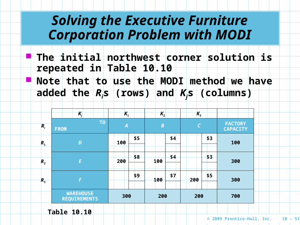
Solving the Executive Furniture Corporation Problem with MODI
The initial northwest corner solution is repeated in Table 10.10
Note that to use the MODI method we have added the Ris (rows) and Kjs (columns)
Kj K1 K2 K3
Ri
TOFROM
A B C FACTORY CAPACITY
R1 D 100$5 $4 $3
100
R2 E 200$8
100$4 $3
300
R3 F$9
100$7
200$5
300
WAREHOUSE REQUIREMENTS 300 200 200 700
Table 10.10

© 2009 Prentice-Hall, Inc. 10 – 54
Solving the Executive Furniture Corporation Problem with MODI
The first step is to set up an equation for each occupied square
By setting R1 = 0 we can easily solve for K1, R2, K2, R3, and K3
(1) R1 + K1 = 5 0 + K1 = 5 K1 = 5
(2) R2 + K1 = 8 R2 + 5 = 8 R2 = 3
(3) R2 + K2 = 4 3 + K2 = 4 K2 = 1
(4) R3 + K2 = 7 R3 + 1 = 7 R3 = 6
(5) R3 + K3 = 5 6 + K3 = 5 K3 = –1

© 2009 Prentice-Hall, Inc. 10 – 55
Solving the Executive Furniture Corporation Problem with MODI
The next step is to compute the improvement index for each unused cell using the formula
Improvement index (Iij) = Cij – Ri – Kj
We have
Des Moines-Boston index
Des Moines-Cleveland index
Evansville-Cleveland index
Fort Lauderdale-Albuquerque index
IDB = C12 – R1 – K2 = 4 – 0 – 1= +$3
IDC = C13 – R1 – K3 = 3 – 0 – (–1)= +$4
IEC = C23 – R2 – K3 = 3 – 3 – (–1)= +$1
IFA = C31 – R3 – K1 = 9 – 6 – 5= –$2

© 2009 Prentice-Hall, Inc. 10 – 56
Solving the Executive Furniture Corporation Problem with MODI
The steps we follow to develop an improved solution after the improvement indices have been computed are
1. Beginning at the square with the best improvement index, trace a closed path back to the original square via squares that are currently being used
2. Beginning with a plus sign at the unused square, place alternate minus signs and plus signs on each corner square of the closed path just traced

© 2009 Prentice-Hall, Inc. 10 – 57
Solving the Executive Furniture Corporation Problem with MODI
3. Select the smallest quantity found in those squares containing the minus signs and add that number to all squares on the closed path with plus signs; subtract the number from squares with minus signs
4. Compute new improvement indices for this new solution using the MODI method Note that new Ri and Kj values must be
calculated Follow this procedure for the second and third
solutions

© 2009 Prentice-Hall, Inc. 10 – 58
Vogel’s Approximation Method: Another Way To Find An Initial Solution
Vogel’s Approximation MethodVogel’s Approximation Method (VAMVAM) is not as simple as the northwest corner method, but it provides a very good initial solution, often one that is the optimaloptimal solution
VAM tackles the problem of finding a good initial solution by taking into account the costs associated with each route alternative
This is something that the northwest corner rule does not do
To apply VAM, we first compute for each row and column the penalty faced if we should ship over the second-bestsecond-best route instead of the least-costleast-cost route
© 2009 Prentice-Hall, Inc. 10 – 59
Vogel’s Approximation Method
The six steps involved in determining an initial VAM solution are illustrated below beginning with the same layout originally shown in Table 10.2
VAM Step 1VAM Step 1. For each row and column of the transportation table, find the difference between the distribution cost on the bestbest route in the row or column and the second bestsecond best route in the row or column
This is the opportunity costopportunity cost of not using the best route
Step 1 has been done in Table 10.11
© 2009 Prentice-Hall, Inc. 10 – 60
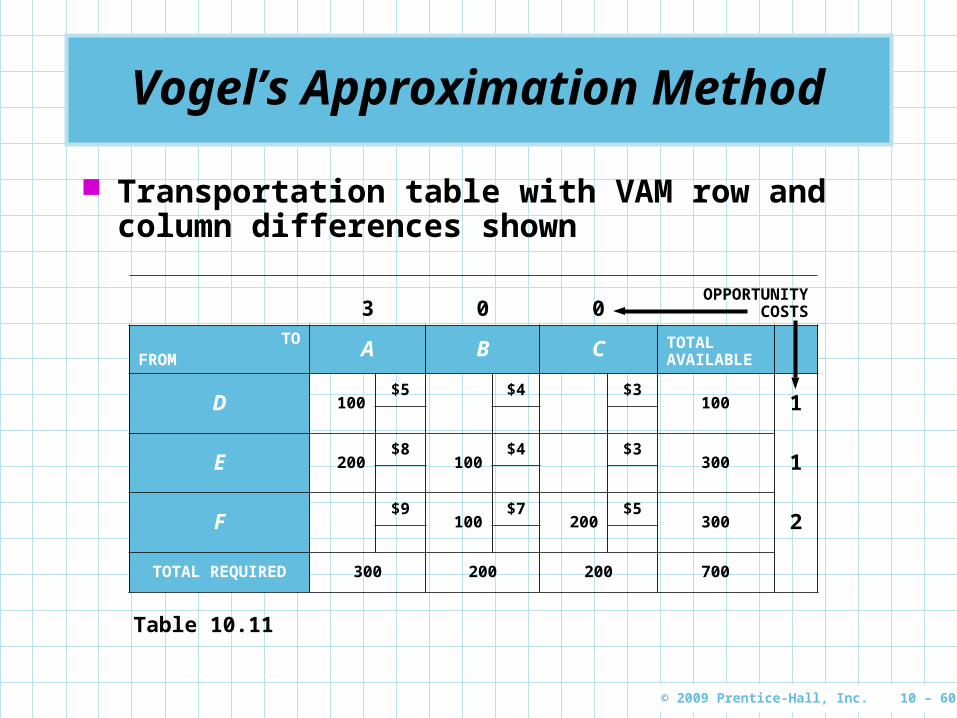
Vogel’s Approximation Method
3 0 0OPPORTUNITY
COSTS
TOFROM A B C TOTAL
AVAILABLE
D 100$5 $4 $3
100 1
E 200$8
100$4 $3
300 1
F$9
100$7
200$5
300 2
TOTAL REQUIRED 300 200 200 700
Table 10.11
Transportation table with VAM row and column differences shown

© 2009 Prentice-Hall, Inc. 10 – 61
Vogel’s Approximation Method
VAM Step 2VAM Step 2. identify the row or column with the greatest opportunity cost, or difference (column A in this example)VAM Step 3VAM Step 3.Assign as many units as possible to the lowest-cost square in the row or column selectedVAM Step 4VAM Step 4. Eliminate any row or column that has been completely satisfied by the assignment just made by placing Xs in each appropriate squareVAM Step 5VAM Step 5. Recompute the cost differences for the transportation table, omitting rows or columns eliminated in the previous step

© 2009 Prentice-Hall, Inc. 10 – 62
Vogel’s Approximation Method
3 1 0 3 0 2OPPORTUNITY
COSTS
TOFROM A B C TOTAL
AVAILABLE
D 100$5
X$4
X$3
100 1
E$8 $4 $3
300 1
F$9 $7 $5
300 2
TOTAL REQUIRED 300 200 200 700
Table 10.12
VAM assignment with D’s requirements satisfied

© 2009 Prentice-Hall, Inc. 10 – 63
Vogel’s Approximation Method
VAM Step 6VAM Step 6. Return to step 2 for the rows and columns remaining and repeat the steps until an initial feasible solution has been obtained
In this case column B now has the greatest difference, 3
We assign 200 units to the lowest-cost square in the column, EB
We recompute the differences and find the greatest difference is now in row E
We assign 100 units to the lowest-cost square in the column, EC

© 2009 Prentice-Hall, Inc. 10 – 64
Vogel’s Approximation Method
Second VAM assignment with B’s requirements satisfied
3 1 0 3 0 2OPPORTUNITY
COSTS
TOFROM A B C TOTAL
AVAILABLE
D 100$5
X$4
X$3
100 1
E$8
200$4 $3
300 1
F$9
X$7 $5
300 2
TOTAL REQUIRED 300 200 200 700
Table 10.13
© 2009 Prentice-Hall, Inc. 10 – 65
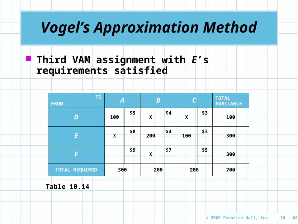
Vogel’s Approximation Method
TOFROM A B C TOTAL
AVAILABLE
D 100$5
X$4
X$3
100
E X$8
200$4
100$3
300
F$9
X$7 $5
300
TOTAL REQUIRED 300 200 200 700
Table 10.14
Third VAM assignment with E’s requirements satisfied

© 2009 Prentice-Hall, Inc. 10 – 66
Vogel’s Approximation Method
TOFROM A B C TOTAL
AVAILABLE
D 100$5
X$4
X$3
100
E X$8
200$4
100$3
300
F 200$9
X$7
100$5
300
TOTAL REQUIRED 300 200 200 700
Table 10.15
Final assignments to balance column and row requirements

© 2009 Prentice-Hall, Inc. 10 – 67
Unbalanced Transportation Problems
In real-life problems, total demand is frequently not equal to total supply
These unbalanced problemsunbalanced problems can be handled easily by introducing dummy sourcesdummy sources or dummy dummy destinationsdestinations
If total supply is greater than total demand, a dummy destination (warehouse), with demand exactly equal to the surplus, is created
If total demand is greater than total supply, we introduce a dummy source (factory) with a supply equal to the excess of demand over supply

© 2009 Prentice-Hall, Inc. 10 – 68
Unbalanced Transportation Problems
In either case, shipping cost coefficients of zero are assigned to each dummy location or route as no goods will actually be shipped
Any units assigned to a dummy destination represent excess capacity
Any units assigned to a dummy source represent unmet demand

© 2009 Prentice-Hall, Inc. 10 – 69
Demand Less Than Supply
Suppose that the Des Moines factory increases its rate of production from 100 to 250 desks
The firm is now able to supply a total of 850 desks each period
Warehouse requirements remain the same (700) so the row and column totals do not balance
We add a dummy column that will represent a fake warehouse requiring 150 desks
This is somewhat analogous to adding a slack variable
We use the northwest corner rule and either stepping-stone or MODI to find the optimal solution

© 2009 Prentice-Hall, Inc. 10 – 70
Demand Less Than Supply
Initial solution to an unbalanced problem where demand is less than supply
TOFROM A B C DUMMY
WAREHOUSETOTAL AVAILABLE
D 250$5 $4 $3 0
250
E 50$8
200$4
50$3 0
300
F$9 $7
150$5
1500
300
WAREHOUSE REQUIREMENTS 300 200 200 150 850
Table 10.16New Des Moines capacity
Total cost = 250($5) + 50($8) + 200($4) + 50($3) + 150($5) + 150(0) = $3,350

© 2009 Prentice-Hall, Inc. 10 – 71
Demand Greater than Supply
The second type of unbalanced condition occurs when total demand is greater than total supply
In this case we need to add a dummy row representing a fake factory
The new factory will have a supply exactly equal to the difference between total demand and total real supply
The shipping costs from the dummy factory to each destination will be zero

© 2009 Prentice-Hall, Inc. 10 – 72
Demand Greater than Supply
Unbalanced transportation table for Happy Sound Stereo Company
TOFROM
WAREHOUSE A
WAREHOUSE B
WAREHOUSE C
PLANT SUPPLY
PLANT W$6 $4 $9
200
PLANT X$10 $5 $8
175
PLANT Y$12 $7 $6
75
WAREHOUSE DEMAND 250 100 150
450500
Table 10.17
Totals do not balance

© 2009 Prentice-Hall, Inc. 10 – 73
Demand Greater than Supply
Initial solution to an unbalanced problem in which demand is greater than supply
TOFROM
WAREHOUSE A
WAREHOUSE B
WAREHOUSE C
PLANT SUPPLY
PLANT W 200$6 $4 $9
200
PLANT X 50$10
100$5
25$8
175
PLANT Y$12 $7
75$6
75
PLANT Y0 0
500
50
WAREHOUSE DEMAND 250 100 150 500
Table 10.18
Total cost of initial solution = 200($6) + 50($10) + 100($5) + 25($8) + 75($6)+ $50(0) = $2,850

© 2009 Prentice-Hall, Inc. 10 – 74
Degeneracy in Transportation Problems
DegeneracyDegeneracy occurs when the number of occupied squares or routes in a transportation table solution is less than the number of rows plus the number of columns minus 1
Such a situation may arise in the initial solution or in any subsequent solution
Degeneracy requires a special procedure to correct the problem since there are not enough occupied squares to trace a closed path for each unused route and it would be impossible to apply the stepping-stone method or to calculate the R and K values needed for the MODI technique

© 2009 Prentice-Hall, Inc. 10 – 75
Degeneracy in Transportation Problems
To handle degenerate problems, create an artificially occupied cell
That is, place a zero (representing a fake shipment) in one of the unused squares and then treat that square as if it were occupied
The square chosen must be in such a position as to allow all stepping-stone paths to be closed
There is usually a good deal of flexibility in selecting the unused square that will receive the zero
© 2009 Prentice-Hall, Inc. 10 – 76
Degeneracy in an Initial Solution
The Martin Shipping Company example illustrates degeneracy in an initial solution
They have three warehouses which supply three major retail customers
Applying the northwest corner rule the initial solution has only four occupied squares
This is less than the amount required to use either the stepping-stone or MODI method to improve the solution (3 rows + 3 columns – 1 = 5)
To correct this problem, place a zero in an unused square, typically one adjacent to the last filled cell
© 2009 Prentice-Hall, Inc. 10 – 77
Degeneracy in an Initial Solution
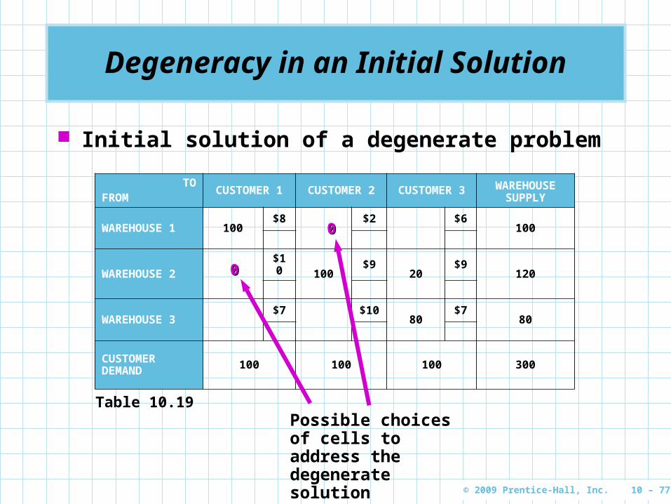
Initial solution of a degenerate problem
TOFROM
CUSTOMER 1 CUSTOMER 2 CUSTOMER 3 WAREHOUSE SUPPLY
WAREHOUSE 1 100$8 $2 $6
100
WAREHOUSE 2$10
100$9
20$9
120
WAREHOUSE 3$7 $10
80$7
80
CUSTOMER DEMAND 100 100 100 300
Table 10.19
00
00
Possible choices of cells to address the degenerate solution
© 2009 Prentice-Hall, Inc. 10 – 78
Degeneracy During Later Solution Stages
A transportation problem can become degenerate after the initial solution stage if the filling of an empty square results in two or more cells becoming empty simultaneously
This problem can occur when two or more cells with minus signs tie for the lowest quantity
To correct this problem, place a zero in one of the previously filled cells so that only one cell becomes empty

© 2009 Prentice-Hall, Inc. 10 – 79
Degeneracy During Later Solution Stages
Bagwell Paint Example After one iteration, the cost analysis at Bagwell
Paint produced a transportation table that was not degenerate but was not optimal
The improvement indices are
factory A – warehouse 2 index = +2factory A – warehouse 3 index = +1factory B – warehouse 3 index = –15factory C – warehouse 2 index = +11
Only route with a negative index

© 2009 Prentice-Hall, Inc. 10 – 80
Degeneracy During Later Solution Stages
Bagwell Paint transportation table
TOFROM
WAREHOUSE 1
WAREHOUSE 2
WAREHOUSE 3
FACTORY CAPACITY
FACTORY A 70$8 $5 $16
70
FACTORY B 50$15
80$10 $7
130
FACTORY C 30$3 $9
50$10
80
WAREHOUSE REQUIREMENT 150 80 50 280
Table 10.20

© 2009 Prentice-Hall, Inc. 10 – 81
Degeneracy During Later Solution Stages
Tracing a closed path for the factory B – warehouse 3 route
TOFROM
WAREHOUSE 1 WAREHOUSE 3
FACTORY B 50$15 $7
FACTORY C 30$3
50$10
Table 10.21
+
+ –
–
This would cause two cells to drop to zero We need to place an artificial zero in one of these
cells to avoid degeneracy

© 2009 Prentice-Hall, Inc. 10 – 82
More Than One Optimal Solution
It is possible for a transportation problem to have multiple optimal solutions
This happens when one or more of the improvement indices zero in the optimal solution
This means that it is possible to design alternative shipping routes with the same total shipping cost
The alternate optimal solution can be found by shipping the most to this unused square using a stepping-stone path
In the real world, alternate optimal solutions provide management with greater flexibility in selecting and using resources

© 2009 Prentice-Hall, Inc. 10 – 83
Maximization Transportation Problems
If the objective in a transportation problem is to maximize profit, a minor change is required in the transportation algorithm
Now the optimal solution is reached when all the improvement indices are negative or zero
The cell with the largest positive improvement index is selected to be filled using a stepping-stone path
This new solution is evaluated and the process continues until there are no positive improvement indices

© 2009 Prentice-Hall, Inc. 10 – 84
Unacceptable Or Prohibited Routes
At times there are transportation problems in which one of the sources is unable to ship to one or more of the destinations
When this occurs, the problem is said to have an unacceptableunacceptable or prohibited routeprohibited route
In a minimization problem, such a prohibited route is assigned a very high cost to prevent this route from ever being used in the optimal solution
In a maximization problem, the very high cost used in minimization problems is given a negative sign, turning it into a very bad profit

© 2009 Prentice-Hall, Inc. 10 – 85
Facility Location Analysis
The transportation method is especially useful in helping a firm to decide where to locate a new factory or warehouse
Each alternative location should be analyzed within the framework of one overalloverall distribution system
The new location that yields the minimum cost for the entire systementire system is the one that should be chosen

© 2009 Prentice-Hall, Inc. 10 – 86
Locating a New Factory for Hardgrave Machine Company
Hardgrave Machine produces computer components at three plants and they ship to four warehouses
The plants have not been able to keep up with demand so the firm wants to build a new plant
Two sites are being considered, Seattle and Birmingham
Data has been collected for each possible location
Which new location will yield the lowest cost for the firm in combination with the existing plants and warehouses

© 2009 Prentice-Hall, Inc. 10 – 87
Locating a New Factory for Hardgrave Machine Company
Hardgrave’s demand and supply data
WAREHOUSE
MONTHLY DEMAND (UNITS)
PRODUCTION PLANT
MONTHLY SUPPLY
COST TO PRODUCE ONE UNIT ($)
Detroit 10,000 Cincinnati 15,000 48
Dallas 12,000 Salt Lake 6,000 50
New York 15,000 Pittsburgh 14,000 52
Los Angeles 9,000 35,000
46,000
Supply needed from new plant = 46,000 – 35,000 = 11,000 units per month
ESTIMATED PRODUCTION COST PER UNIT AT PROPOSED PLANTS
Seattle $53
Birmingham $49
Table 10.22

© 2009 Prentice-Hall, Inc. 10 – 88
Locating a New Factory for Hardgrave Machine Company
Hardgrave’s shipping costs
TOFROM DETROIT DALLAS NEW YORK
LOS ANGELES
CINCINNATI $25 $55 $40 $60
SALT LAKE 35 30 50 40
PITTSBURGH 36 45 26 66
SEATTLE 60 38 65 27
BIRMINGHAM 35 30 41 50
Table 10.23

© 2009 Prentice-Hall, Inc. 10 – 89
Locating a New Factory for Hardgrave Machine Company
Optimal solution for the Birmingham location
TOFROM DETROIT DALLAS NEW YORK
LOS ANGELES
FACTORY CAPACITY
CINCINNATI 10,00073 103
1,00088
4,000108
15,000
SALT LAKE85
1,00080 100
5,00090
6,000
PITTSBURGH88 97
14,00078 118
14,000
BIRMINGHAM84
11,00079 90 99
11,000
WAREHOUSE REQUIREMENT 10,000 12,000 15,000 9,000 46,000
Table 10.24

© 2009 Prentice-Hall, Inc. 10 – 90
Locating a New Factory for Hardgrave Machine Company
Optimal solution for the Seattle location
TOFROM DETROIT DALLAS NEW YORK
LOS ANGELES
FACTORY CAPACITY
CINCINNATI 10,00073
4,000103
1,00088 108
15,000
SALT LAKE85
6,00080 100 90
6,000
PITTSBURGH88 97
14,00078 118
14,000
SEATTLE113
2,00091 118
9,00080
11,000
WAREHOUSE REQUIREMENT 10,000 12,000 15,000 9,000 46,000
Table 10.25
© 2009 Prentice-Hall, Inc. 10 – 91
Locating a New Factory for Hardgrave Machine Company
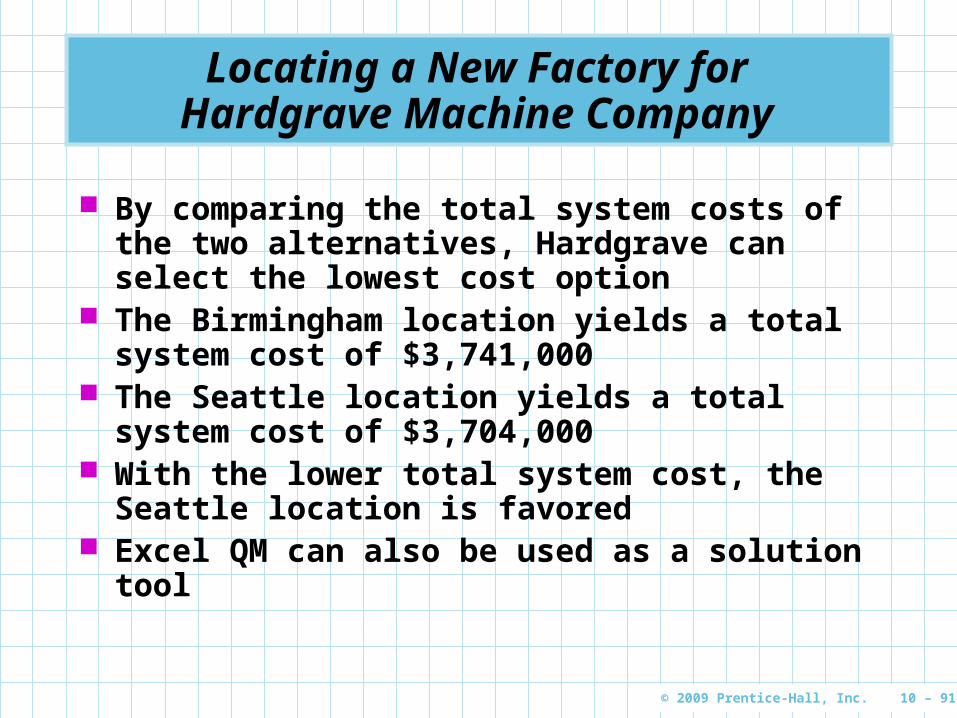
By comparing the total system costs of the two alternatives, Hardgrave can select the lowest cost option
The Birmingham location yields a total system cost of $3,741,000
The Seattle location yields a total system cost of $3,704,000
With the lower total system cost, the Seattle location is favored
Excel QM can also be used as a solution tool
© 2009 Prentice-Hall, Inc. 10 – 92
Locating a New Factory for Hardgrave Machine Company
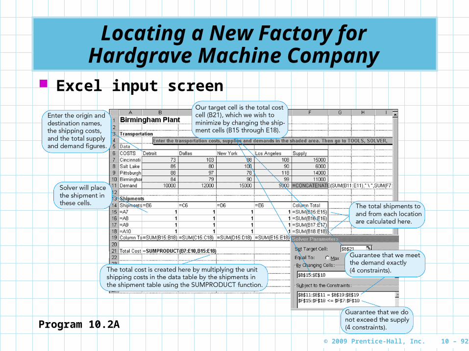
Excel input screen
Program 10.2A

© 2009 Prentice-Hall, Inc. 10 – 93
Locating a New Factory for Hardgrave Machine Company
Output from Excel QM analysis
Program 10.2A

© 2009 Prentice-Hall, Inc. 10 – 94
Assignment Model Approach
The second special-purpose LP algorithm is the assignment method
Each assignment problem has associated with it a table, or matrix
Generally, the rows contain the objects or people we wish to assign, and the columns comprise the tasks or things we want them assigned to
The numbers in the table are the costs associated with each particular assignment
An assignment problem can be viewed as a transportation problem in which the capacity from each source is 1 and the demand at each destination is 1

© 2009 Prentice-Hall, Inc. 10 – 95
Assignment Model Approach
The Fix-It Shop has three rush projects to repair They have three repair persons with different
talents and abilities The owner has estimates of wage costs for each
worker for each project The owner’s objective is to assign the three
project to the workers in a way that will result in the lowest cost to the shop
Each project will be assigned exclusively to one worker
© 2009 Prentice-Hall, Inc. 10 – 96
Assignment Model Approach
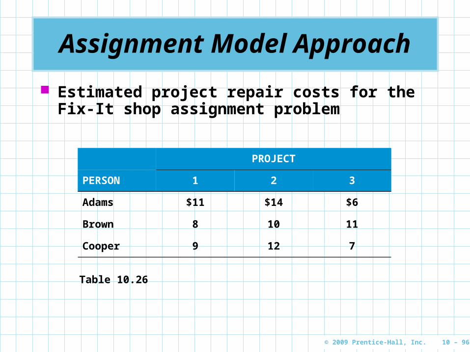
Estimated project repair costs for the Fix-It shop assignment problem
PROJECT
PERSON 1 2 3
Adams $11 $14 $6
Brown 8 10 11
Cooper 9 12 7
Table 10.26

© 2009 Prentice-Hall, Inc. 10 – 97
Assignment Model Approach
Summary of Fix-It Shop assignment alternatives and costs
PRODUCT ASSIGNMENT
1 2 3 LABOR COSTS ($)
TOTAL COSTS ($)
Adams Brown Cooper 11 + 10 + 7 28
Adams Cooper Brown 11 + 12 + 11 34
Brown Adams Cooper 8 + 14 + 7 29
Brown Cooper Adams 8 + 12 + 6 26
Cooper Adams Brown 9 + 14 + 11 34
Cooper Brown Adams 9 + 10 + 6 25
Table 10.27

© 2009 Prentice-Hall, Inc. 10 – 98
The Hungarian Method (Flood’s Technique)
The Hungarian methodHungarian method is an efficient method of finding the optimal solution to an assignment problem without having to make direct comparisons of every option
It operates on the principle of matrix reductionmatrix reduction By subtracting and adding appropriate numbers
in the cost table or matrix, we can reduce the problem to a matrix of opportunity costsopportunity costs
Opportunity costs show the relative penalty associated with assigning any person to a project as opposed to making the bestbest assignment
We want to make assignment so that the opportunity cost for each assignment is zero

© 2009 Prentice-Hall, Inc. 10 – 99
Three Steps of the Assignment Method
1.1. Find the opportunity cost table byFind the opportunity cost table by:(a) Subtracting the smallest number in each row
of the original cost table or matrix from every number in that row
(b) Then subtracting the smallest number in each column of the table obtained in part (a) from every number in that column
2.2. Test the table resulting from step 1 to see Test the table resulting from step 1 to see whether an optimal assignment can be madewhether an optimal assignment can be made by drawing the minimum number of vertical and horizontal straight lines necessary to cover all the zeros in the table. If the number of lines is less than the number of rows or columns, proceed to step 3.

© 2009 Prentice-Hall, Inc. 10 – 100
Three Steps of the Assignment Method
3.3. Revise the present opportunity cost tableRevise the present opportunity cost table by subtracting the smallest number not covered by a line from every other uncovered number. This same number is also added to any number(s) lying at the intersection of horizontal and vertical lines. Return to step 2 and continue the cycle until an optimal assignment is possible.

© 2009 Prentice-Hall, Inc. 10 – 101
Test opportunity cost table to see if optimal assignments are possible by drawing the minimum possible lines on columns and/or rows such that all zeros are covered
Find opportunity cost(a) Subtract smallest number in
each row from every number in that row, then
(b) subtract smallest number in each column from every number in that column
Steps in the Assignment Method
Set up cost table for problem Revise opportunity cost table in two steps:(a) Subtract the smallest number not covered by a line from itself and every other uncovered number(b) add this number at every intersection of any two lines
Optimal solution at zero locations. Systematically make final assignments.(a) Check each row and column for a unique zero and make the first assignment in that row or column(b) Eliminate that row and column and search for another unique zero. Make that assignment and proceed in a like manner.
Step 1
Not optimal
Step 2
Optimal
Figure 10.3
© 2009 Prentice-Hall, Inc. 10 – 102
The Hungarian Method (Flood’s Technique)
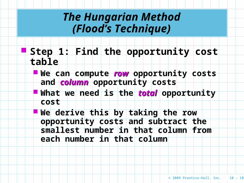
Step 1: Find the opportunity cost table We can compute rowrow opportunity costs and
columncolumn opportunity costs What we need is the totaltotal opportunity cost We derive this by taking the row opportunity
costs and subtract the smallest number in that column from each number in that column

© 2009 Prentice-Hall, Inc. 10 – 103
The Hungarian Method (Flood’s Technique)
Cost of each person-project assignment
Row opportunity cost table
PROJECT
PERSON 1 2 3
Adams $11 $14 $6
Brown 8 10 11
Cooper 9 12 7
Table 10.28
PROJECT
PERSON 1 2 3
Adams $5 $8 $0
Brown 0 2 3
Cooper 2 5 0
Table 10.29
The opportunity cost of assigning Cooper to project 2 is $12 – $7 = $5

© 2009 Prentice-Hall, Inc. 10 – 104
The Hungarian Method (Flood’s Technique)
We derive the total opportunity costs by taking the costs in Table 29 and subtract the smallest number in each column from each number in that column
Row opportunity cost table
PROJECT
PERSON 1 2 3
Adams $5 $8 $0
Brown 0 2 3
Cooper 2 5 0
Table 10.29
Total opportunity cost table
PROJECT
PERSON 1 2 3
Adams $5 $6 $0
Brown 0 0 3
Cooper 2 3 0
Table 10.30
© 2009 Prentice-Hall, Inc. 10 – 105
The Hungarian Method (Flood’s Technique)
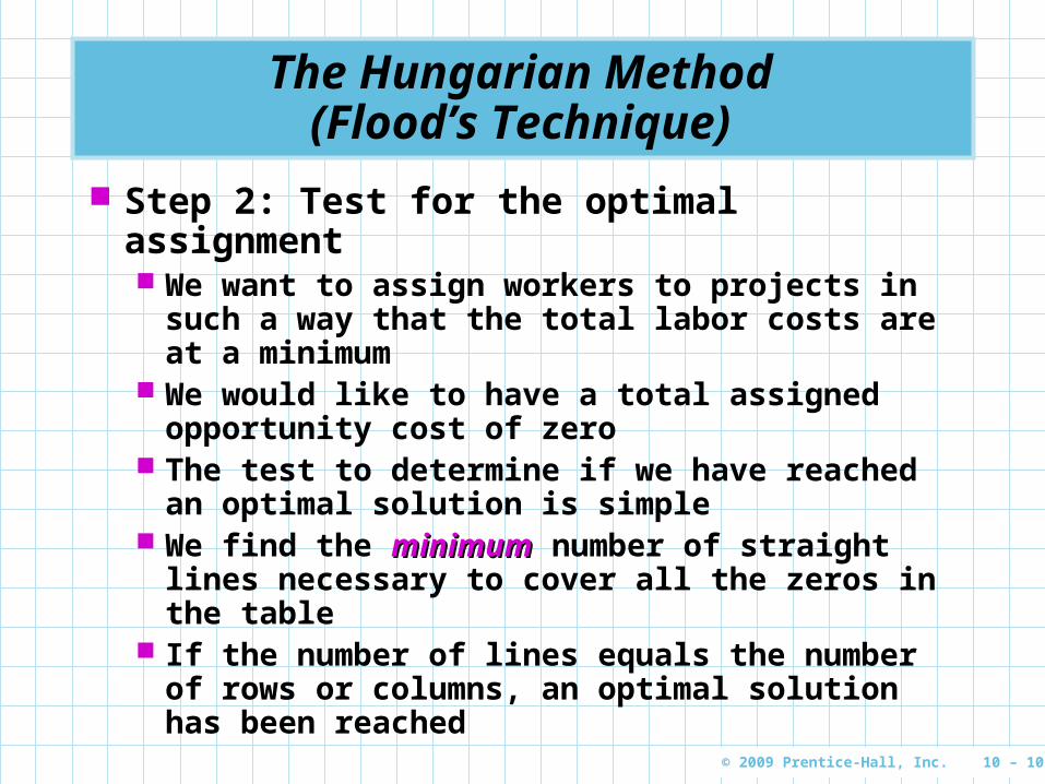
Step 2: Test for the optimal assignment We want to assign workers to projects in such
a way that the total labor costs are at a minimum
We would like to have a total assigned opportunity cost of zero
The test to determine if we have reached an optimal solution is simple
We find the minimumminimum number of straight lines necessary to cover all the zeros in the table
If the number of lines equals the number of rows or columns, an optimal solution has been reached

© 2009 Prentice-Hall, Inc. 10 – 106
The Hungarian Method (Flood’s Technique)
Test for optimal solution
PROJECT
PERSON 1 2 3
Adams $5 $6 $0
Brown 0 0 3
Cooper 2 3 0
Table 10.31
Covering line 1Covering line 1
Covering line 2Covering line 2
This requires only two lines to cover the zeros so the solution is not optimal
© 2009 Prentice-Hall, Inc. 10 – 107
The Hungarian Method (Flood’s Technique)
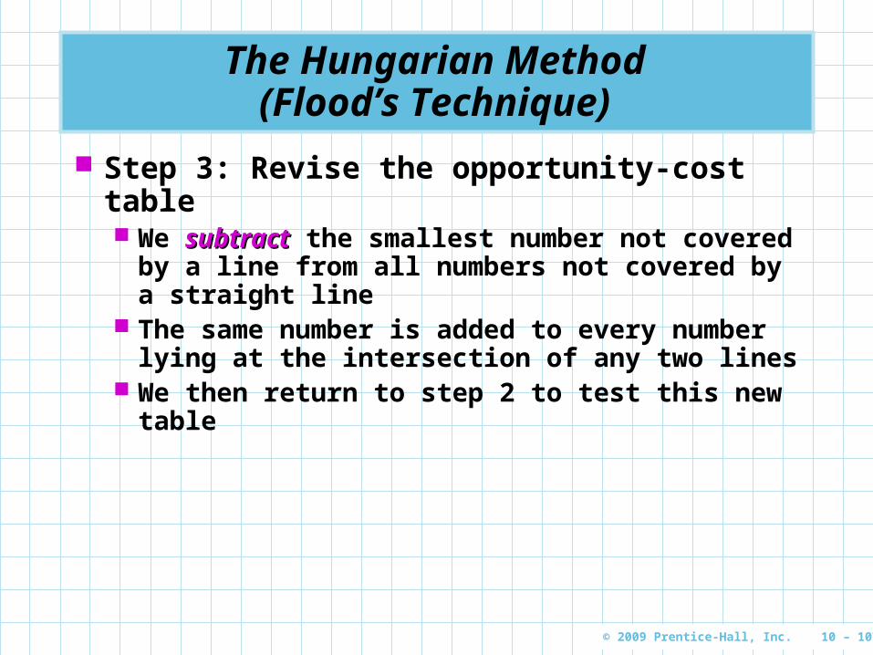
Step 3: Revise the opportunity-cost table We subtractsubtract the smallest number not covered
by a line from all numbers not covered by a straight line
The same number is added to every number lying at the intersection of any two lines
We then return to step 2 to test this new table
© 2009 Prentice-Hall, Inc. 10 – 108
The Hungarian Method (Flood’s Technique)
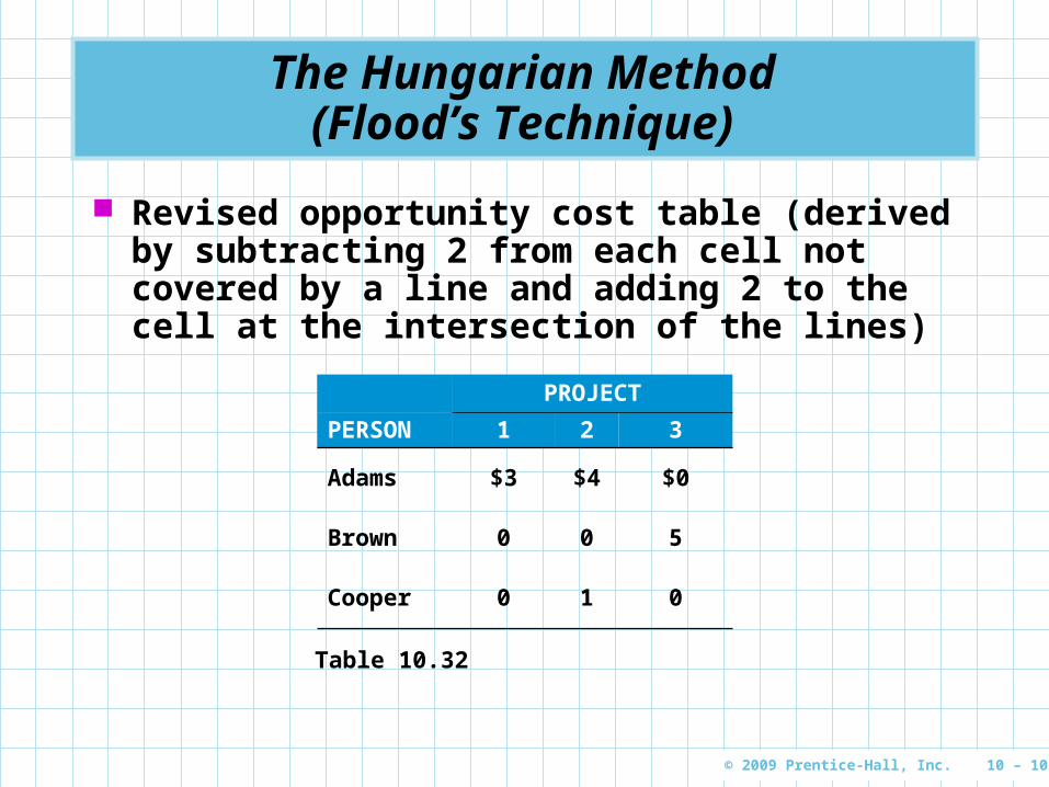
Revised opportunity cost table (derived by subtracting 2 from each cell not covered by a line and adding 2 to the cell at the intersection of the lines)
PROJECT
PERSON 1 2 3
Adams $3 $4 $0
Brown 0 0 5
Cooper 0 1 0
Table 10.32
© 2009 Prentice-Hall, Inc. 10 – 109
The Hungarian Method (Flood’s Technique)
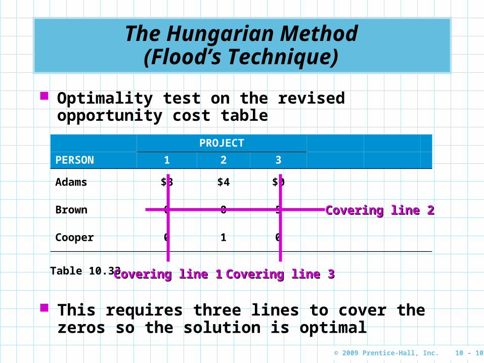
Optimality test on the revised opportunity cost table
PROJECT
PERSON 1 2 3
Adams $3 $4 $0
Brown 0 0 5
Cooper 0 1 0
Table 10.33
Covering line 2Covering line 2
Covering line 3Covering line 3
This requires three lines to cover the zeros so the solution is optimal
Covering line 1Covering line 1

© 2009 Prentice-Hall, Inc. 10 – 110
Making the Final Assignment
The optimal assignment is Adams to project 3, Brown to project 2, and Cooper to project 1
But this is a simple problem For larger problems one approach to making the
final assignment is to select a row or column that contains only one zero
Make the assignment to that cell and rule out its row and column
Follow this same approach for all the remaining cells

© 2009 Prentice-Hall, Inc. 10 – 111
Making the Final Assignment
Total labor costs of this assignment are
ASSIGNMENT COST ($)
Adams to project 3 6
Brown to project 2 10
Cooper to project 1 9
Total cost 25

© 2009 Prentice-Hall, Inc. 10 – 112
Making the Final Assignment
Making the final assignments
(A) FIRST ASSIGNMENT
(B) SECOND ASSIGNMENT
(C) THIRD ASSIGNMENT
1 2 3 1 2 3 1 2 3
Adams 3 4 0 Adams 3 4 0 Adams 3 4 0
Brown 0 0 5 Brown 0 0 5 Brown 0 0 5
Cooper 0 1 0 Cooper 0 1 0 Cooper 0 1 0
Table 10.34

© 2009 Prentice-Hall, Inc. 10 – 113
Using Excel QM for the Fix-It Shop Assignment Problem
Excel QM assignment module
Program 10.3A

© 2009 Prentice-Hall, Inc. 10 – 114
Using Excel QM for the Fix-It Shop Assignment Problem
Excel QM output screen
Program 10.3A

© 2009 Prentice-Hall, Inc. 10 – 115
Unbalanced Assignment Problems
Often the number of people or objects to be assigned does not equal the number of tasks or clients or machines listed in the columns, and the problem is unbalancedunbalanced
When this occurs, and there are more rows than columns, simply add a dummy columndummy column or task
If the number of tasks exceeds the number of people available, we add a dummy rowdummy row
Since the dummy task or person is nonexistent, we enter zeros in its row or column as the cost or time estimate
© 2009 Prentice-Hall, Inc. 10 – 116
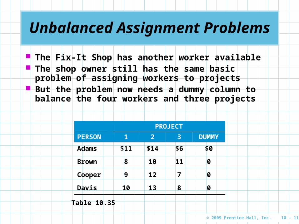
Unbalanced Assignment Problems
The Fix-It Shop has another worker available The shop owner still has the same basic problem
of assigning workers to projects But the problem now needs a dummy column to
balance the four workers and three projects
PROJECT
PERSON 1 2 3 DUMMY
Adams $11 $14 $6 $0
Brown 8 10 11 0
Cooper 9 12 7 0
Davis 10 13 8 0
Table 10.35

© 2009 Prentice-Hall, Inc. 10 – 117
Maximization Assignment Problems
Some assignment problems are phrased in terms of maximizing the payoff, profit, or effectiveness
It is easy to obtain an equivalent minimization problem by converting all numbers in the table to opportunity costs
This is brought about by subtracting every number in the original payoff table from the largest single number in that table
Transformed entries represent opportunity costs Once the optimal assignment has been found, the
total payoff is found by adding the original payoffs of those cells that are in the optimal assignment

© 2009 Prentice-Hall, Inc. 10 – 118
Maximization Assignment Problems
The British navy wishes to assign four ships to patrol four sectors of the North Sea
Ships are rated for their probable efficiency in each sector
The commander wants to determine patrol assignments producing the greatest overall efficiencies

© 2009 Prentice-Hall, Inc. 10 – 119
Maximization Assignment Problems
Efficiencies of British ships in patrol sectors
SECTOR
SHIP A B C D
1 20 60 50 55
2 60 30 80 75
3 80 100 90 80
4 65 80 75 70
Table 10.36

© 2009 Prentice-Hall, Inc. 10 – 120
Maximization Assignment Problems
Opportunity cost of British ships
SECTOR
SHIP A B C D
1 80 40 50 45
2 40 70 20 25
3 20 0 10 20
4 35 20 25 30
Table 10.37
© 2009 Prentice-Hall, Inc. 10 – 121
Maximization Assignment Problems
First convert the maximization efficiency table into a minimizing opportunity cost table by subtracting each rating from 100, the largest rating in the whole table
The smallest number in each row is subtracted from every number in that row and the smallest number in each column is subtracted from every number in that column
The minimum number of lines needed to cover the zeros in the table is four, so this represents an optimal solution

© 2009 Prentice-Hall, Inc. 10 – 122
Maximization Assignment Problems
The overall efficiency
ASSIGNMENT EFFICIENCY
Ship 1 to sector D 55
Ship 2 to sector C 80
Ship 3 to sector B 100
Ship 4 to sector A 65
Total efficiency 300