Trajectory Planning and Lateral Control forAgricultural Guidance Applications

Patrick Fleischmann∗, Tobias Fohst∗ and Karsten Berns∗∗Robotics Research Lab, Department of Computer Science

University of Kaiserslautern, 67663 Kaiserslautern, GermanyEmail: {fleischmann,foehst,berns}@cs.uni-kl.de

Abstract—This paper addresses a planning approach basedon B-splines for successively generated trajectories. Additionally,the lateral controller which was used to calculate the steeringangle is described and the method how the required parameterswere determined is introduced. It is explained how the outputof a perception system is used to generate control points for thetrajectory and how the inputs of the path tracker are derivedfrom the B-splines which are represented as Bezier curves. Theperformance of the planning and control approach was tested ontwo different agricultural machines and also within a windrowguidance application.

I. INTRODUCTION

At present, nearly every existing automatic guidance sys-tem for agricultural vehicles like tractors, sprayers or har-vesters is based on global navigation satellite systems (GNSS)like the NAVSTAR-GPS. The majority of manufacturers offerthese solutions like the StarFire system by John Deere, theGPS PILOT by Claas or the EZ-GUidE products of NewHolland to name only some examples. To achieve the accuracyrequired for agricultural applications, correction signals areused to improve the localization quality up to ±2 cm. Besidecost-free satellite based augmentation systems like EGNOS orWAAS, the manufacturers additionally offer correction signals(StarFire SF1/SF2, OmniSTAR XP/HP) or RTK based systemswhich are subject to licensing. All these GNSS based systemshave to deal with some main drawbacks although they are verysuccessful on the market. Weak spots are that the localizationrobustness depends on structures like trees, building, bridgesetc. in the environment which shadow the satellite connectionand that the tracks have to be pre-recorded or calculated bycalibrated control points. Other disadvantages beside the hard-ware and licensing costs are that these systems are not capableof following already existing structures such as orchards, plantrows, windrows, or cut edges as well as the inability to handleobstacles or changed environmental conditions.

These drawbacks lead us to focus on agricultural guidancesolutions where GNSS sensors are not required or supportedby other, more cost effective or reliable sensors which mapthe environment. As a first demonstrating application a modeldriven windrow detection based on a laser scanner was de-veloped during the last two years. To steer the tractor andthe implement in a smooth way and to keep both above thewindrow we have identified that calculating the steering anglebased on the immediate output of the sensor is not reliable,especially for higher velocities. This is because the outputof the detection is not robust enough as the appearance andquantity of the straw varies to much. Additionally, a calculation

of the required steering angle only based on the output ofthe sensor requires a specific position of the device to handlethe delays of the steering actuator. Especially in curves it isvery difficult to distinguish between outliers and correct valuesbecause of the very local view. In addition, our target was toreach velocities up to 20 km/h and in this case it was not possibleto achieve a smooth path which is comfortable for the driveras well as suitable for the mechanics of the steering.

To solve these difficulties a trajectory planner was imple-mented which is able to handle the successive extension ofthe path, which creates an output that is smooth enough evenfor higher velocities and which is able to reduce the influenceof outliers or detection failures. Due to the requirements aB-spline based approach was selected and implemented asBezier curves because of the advantages of this representation.Furthermore, a lateral controller was designed to keep thetractor on the trajectory which is also subject of this paper.

In computer graphics Bezier curves are widely used be-cause of their numerous positive features e.g. the convexhull property which can be used for an efficient intersectioncalculation or a subdivision algorithm which can improve thedrawing of a curve [1]. Another important attribute which isvery interesting for robotic applications is that a Bezier curve– in contrast to a polynomial interpolation – will interpolatepoints which lie on a straight line as a line segment. Thedrawback that the modification of a single control point altersthe whole curve can be solved by the usage of B-splines wherethe changes are limited to a given number of segments. [2]shows an approach for a small electric car where a Beziercurve based path planner is used to alter a pre-defined path ifits blocked by an obstacle. A similar research issue is contentof [3] where a B-spline is used to create a trajectory inside anindoor environment which can be locally and thus efficientlymodified if the pre-calculated path is blocked. [4] describesa spline based path planning algorithm for the outdoor robotOverbot which was a participant of the DARPA Grand Chal-lenge. Here, 3 pre-defined GPS waypoints are interpolated ateach time by a cubic spline to generate a trajectory. If the pathis obstructed, additional control points next to the obstacle areinserted until a collision free path is found.

For autonomous road vehicles the path tracking problemhas also been a subject to numerous approaches. Especiallythe DARPA Grand and Urban Challenges have pushed thedevelopment of various lateral controllers. Maybe the mostfamous one is presented in [5] where a nonlinear feedbackfunction of the cross-track and orientation error at the frontaxle is used to calculate the steering angle. The controller

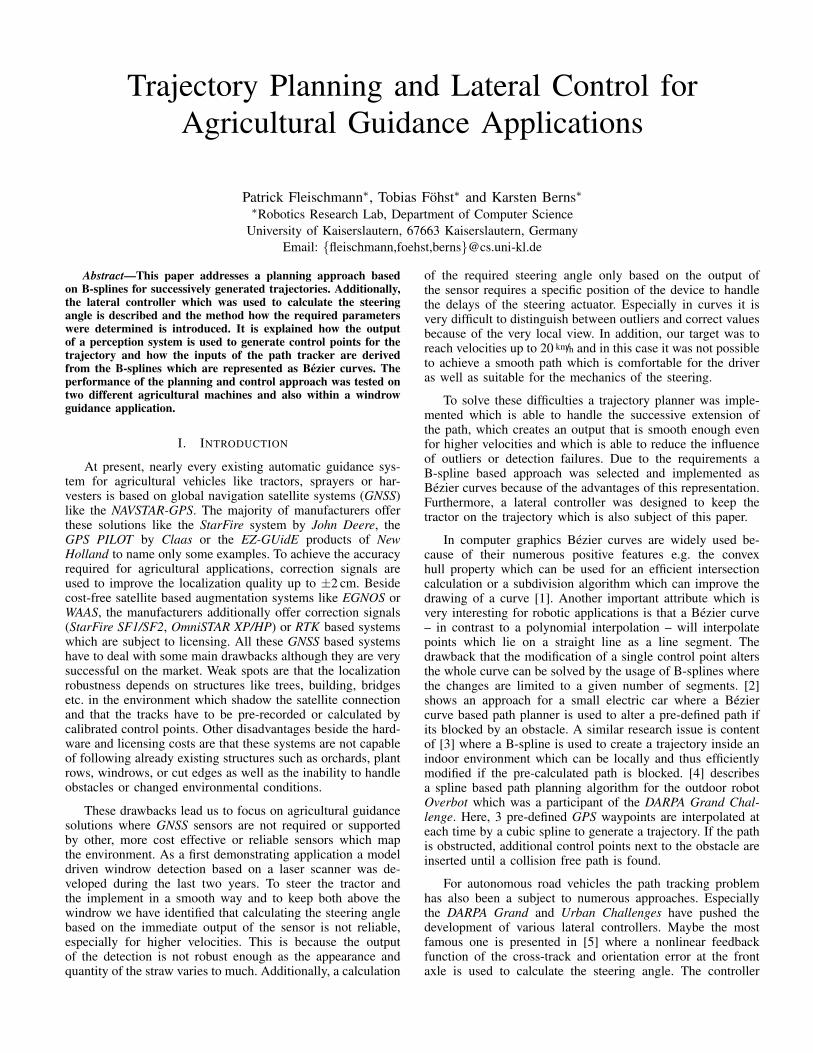
Fig. 1. Application scenario: Tractor with a large round baler following awindrow while collecting the material

presented [6] was also developed for an autonomous carwith Ackermann kinematics and determines the output bycomparing the vehicle’s current position and orientation witha virtual reference vehicle which drives on the trajectory. Agood overview of different types of lateral controllers startingfrom simple geometric path trackers to controllers which havea underlying kinematic or dynamic model of the vehicleas well as their capabilities and limitations is given in [7].Path trackers for tractors are e.g. described in [8] where asimple Pure Pursuit controller is used and tested for velocitiesup to 8 km/h. Unfortunately, this type of controller is limitedto lower speeds as the vehicle dynamics will influence theperformance for higher velocities. Various experiments haveshown that controllers which rely on a dynamic model easilyoutperform simple geometric controllers. But a main drawbackof those systems is the complexity and the requirement ofmany parameters that are in some cases very difficult toidentify. For a tractor interesting approaches are describedin [9]–[10] where the controller tries to compensate for thesliding of the farm vehicle. Here, e.g. the cornering stiffnessof the tires is estimated by the controller itself which is a verypromising method as this parameter is usually very difficult toidentify.

II. APPLICATION SCENARIO

The trajectory planner and lateral controller which are con-tent of this paper are part of a demonstrator for a model baseddetection approach for typical structures in the agriculturalenvironment. Since the described drawbacks of GNSS-basedsteering systems should be avoided, the developed assistancesystem exclusively relies on distance data information of asingle line laser scanner which is additionally robust againstvarying illumination. This guidance application for a tractorwas designed to follow windrows (rows of cut or mowed croplike hay, straw, or silage) in order to collect the material usinga baler. The most common type of baler which was also usedduring the experiments is the large round baler. This devicecollects the crop using a so-called pick-up, compresses thematerial in a round chamber, and wraps the bale with a meshwhen the chamber is filled. Due to the fact that the collectionmechanism has a limited width and that the crop is taken intothe chamber as it is, the farm machine has to be driven almostcentered over the swath to get a homogeneous shaped bale.Fig. 1 illustrates a tractor together with its implement duringthis task.

III. TRAJECTORY GENERATION USING B-SPLINES

The input for the trajectory planner is the output of thedetection module which delivers a so-called guidance pointin the tractor fixed reference frame which is originated on theground below the rear axis of the tractor. For the experiments adistance of around 11.5 m in front of the rear axis was selectedfor the guidance point which varies with the surface of theground, the shape of the windrow and which can be modifiedthrough the mounting position and angle of the sensor. As afirst step, these guidance points are converted into a worldfixed 2D coordinate system (WCS) which is set up duringthe start of the system. To convert the point to the WCSthe position and orientation of the tractor is required whichis determined by using an IMU and the wheel speed signalof the tractor. It is obvious that this localization is stronglyerror prone after a while due to the error accumulation ofthe IMU and the inaccuracies of the wheel velocities. But asthe tractor follows an existing structure, only a roughly validlocalization is required for the next couple of meters to createa trajectory. In addition to this conversion, every incomingguidance point is evaluated according its drivability which islimited to a speed dependent maximal desired steering angle.This mechanism allows to drive sharp curves for low velocitiesand reduces unwanted amplitudes for higher velocities and alsoremoves outliers. Furthermore, not every point is taken as awaypoint for the trajectory since many close control points forthe spline would lead to a very varying and oscillating pathas the output of the detection is influenced by vibrations ofthe tractor, the nature of the surface, the noise of the sensorand the uncertainty of the probabilistic processing algorithm.To handle this a parameterized (Euclidean) distance betweentwo waypoints must be exceeded until the point is added as acontrol point (see also Fig. 3).

Driving along these predefined waypoints can be easilyimplemented by moving to the first point in the list and usingstraight lines from each waypoint to its successor. However,driving with an implement and especially at higher speedsneeds a smooth parametric curved trajectory that allows errorestimation for the current position and orientation even whileapproaching the curve and transitioning from one point to theother. Therefore, polynomial curves can be fit into the set ofwaypoints to define a smooth trajectory.

The typical stability issues with polynomials of higherdegree can be avoided by looking only at a reduced localset of waypoints, ignoring already passed points and possiblylimiting the foresight of the controller. Alternatively, the tra-jectory can be defined as a complete spline composed of localcurves of lower degree. Additionally, the proposed methoduses Bezier polygons to represent the polynomials due to theirgood numerical stability and fast algorithms for evaluation,derivation and drawing [1].

A. Bezier curves

Every polynomial curve can be represented using its so-called Bezier polygon. The curve and the polygon share theirend points and end tangents and the curve lies within theconvex hull of the Bezier polygon.

Applying the Bernstein polynomials

Bni (t) =

(n

i

)ti (1− t)n−i , i = 0, . . . , n

a Bezier polygon consisting of n+ 1 control points ci definesa polynomial parametric curve s (t) of degree ≤ n with 0 ≤t ≤ 1 (see Fig. 2).

s(t)

c01

c10

c00

c02

c12

c03

c11

c20

c30

c21

Fig. 2. The de Casteljau construction of s(t) and the resulting subdivisionof a cubic Bezier polygon

B. The de Casteljau algorithm

A curve

s (t) =

n∑i=0

ciBni (t)

can be easily evaluated using the de Casteljau algorithm [11]:From the identity(

n+ 1

i

)=

(n

i− 1

)+

(n

i

)follows the recursion formula for Bernstein polynomials:

Bn+1i (t) = tBni−1 (t) + (1− t)Bni (t)

with Bn−1 = Bnn+1 = 0 and B00 = 1. Hence, the curve also

has a recursive formula:

s (t) =

n∑i=0

c0iB

ni (t)

=

n−1∑i=0

c1iB

n−1i (t) = . . . =

0∑i=0

cni B0i (t) = cn0

with ck+1i = (1− t) cki + tcki+1, c0

i = ci

C. Subdivision, intersections, closest points and drawing

Applying the de Casteljau algorithm with an arbitraryparameter 0 ≤ t ≤ 1 not only evaluates s (t) but alsosubdivides s at t into two new Bezier curves with controlpoints

{c0

0, c10, . . . , c

n0

}and

{cn0 , c

n−11 , . . . , c0

n

}(Fig. 2). The

twist of the curve (maximum of second derivative) measuresthe flatness of s and can therefore be used as criterion whenthe curve can be approximated by its baseline between thefirst and last control point. Hence, geometric operations likeintersecting with other curves or lines, finding the closest pointon the curve to a reference point, etc. can be reduced to lineoperations after iteratively subdividing s. Even visualizing thecurve can be implemented by drawing lines after subdividingdepending on the current scaling (resolution) of the image.

The implementation of these algorithms benefits from theconvex hull property of Bezier curves and can therefore avoidunnecessary subdivisions of unaffected regions of s.

D. Derivatives

To compute the orientation and curvature at a specific pointon the curve s(t) the first and second derivatives must becalculated. The derivative of a Bernstein polynomial of degreen is

∂

∂tBni (t) = n

(Bn−1i−1 (t)−Bn−1

i (t)), Bn−1

−1 = Bn−1n = 0

Thus, the derivative s′(t) is obtained by

∂

∂ts(t) = n

n−1∑i=0

∆ciBn−1i (t) with ∆ci = ci+1 − ci

This makes the first derivative of s again a Bezier curve ofdegree n−1 with control points n∆c0, . . . , n∆cn. The secondand further derivatives can be obtained recursively.

E. B-splines

Depending on the density and noise of the generatedwaypoints the generated spline curve can interpolate or approx-imate the waypoints. Interpolation means each point is hit bythe trajectory whereas approximation means that the generatedcurves are within a wider path spanned by the waypoints. Thelatter has an additional filtering effect that smooths out smallerinstabilities of waypoint locations.

To create a spline curve, basis functions can be used asweights for a linear combination of the control points likein Bezier curves. While the basis functions of Bezier curves(Bernstein polynomials) are non-zero over the whole domain,a spline needs more local functions. This is achieved byintroducing a knot vector with elements ui and basis functionsthat are non-zero for adjacent subintervals of that knot vector,using the Cox-de Boor recursion formula:

N0i (u) =

{1 if ui ≤ u < ui+1

0 otherwise

Nni (u) =

u− uiui+n − ui

Nn−1i (u) +

ui+n+1 − uui+n+1 − ui+1

Nn−1i+1 (u)

Hence, a B-spline basis function Nni (u) is non-zero on

[ui, ui+n+1), defining the locality of the control points’ influ-ence on the curve.

From that definition, a B-spline of degree n with m controlpoints needs a knot vector of length n+m+1. Satisfying thisrequirement means to add start and end conditions that fix thefirst and last segments that do not have enough neighbors toone side, e.g. by a uniform knot vector in the domain [0, 1]with multiple knots at 0 and 1:

(u0 = . . . = un, un+1, . . . , um, um+1 = . . . = um+n)

=(

0, . . . , 0, 1m−1 , . . . ,

m−2m−1 , 1, . . . , 1

)

F. Knot insertion

One important algorithm for B-splines is knot insertion.That is inserting new knots into the knot vector togetherwith according control points and transforming the existingcontrol points so that the shape of the spline curve doesnot change. Inserting u into u = (u0, . . . , ul, ul+1, . . .) gives

v = (u0, . . . , ul, u, ul+1, . . .) andm−1∑i=0

ciNni (u) becomes

m∑i=0

ciNni (v) with the new control points

ci = (1− αi) ci−1 + αici

αi =

1 if i ≤ l − n0 if i > lu−ui

ul+n−uielse

Doing that, the multiplicity of each inner knot can beincreased until the affected basis functions for each segmentequal to the Bernstein polynomials in the according localdomain. Then, the new control points that are involved inshaping a segment become Bezier control points for thatparticular local curve.

IV. LATERAL CONTROLLER

In order to steer the tractor along the calculated trajectory, aso-called lateral controller can be used to calculate the requiredsteering angles. The controller which was implemented for thattask uses up to 3 factors which are derived according the actualposition of the robot and the current trajectory. As shown inFig. 3, a velocity dependent look-ahead point l(t) is determinedwhich lies on the y-axis of the tractor fixed coordinate system(RCS). The point can be found by evaluating the followingequation:

l(t)(RCS) = (lb + lv · v(t), 0)T (1)

where lb is a vehicle dependent, constant addend whichshould not be set smaller then the wheelbase of the vehicle.To consider the delay of the communication with the steeringsystem, which has a certain reaction time, the value couldbe additionally increased. Additionally, the steering actuatorneeds some time to realize the given steering angle. This resultsinto the requirement that the look-ahead point needs to befarther away from the vehicle for higher speeds to be able torealize the angle in time. In (1) this is modeled by a velocity-dependent part which consists of a factor lv and the currentvelocity v(t) of the vehicle.

After transforming the look-ahead point into the WCS byemploying the current location of the tractor the first stepis to determine the closest point p(t) on the B-spline (seesection III-C). This point has the shortest distance from thetrajectory to the look-ahead point l(t)(WCS). Once this pointis found – this is done by subdividing the B-spline into smallpieces which can be linearized afterwards without introducinga large error – the lateral error de(t) can be easily computed asthe distance between p(t) and l(t)(WCS). This error, which isalso known as cross track error, indicates how far the vehiclewould differ from the trajectory at the look-ahead point if thecurrent orientation of the vehicle would be maintained (thevehicle would go straight).

de(t)

xRCS

θe(t)

l(t)

yRCS

lb + lv · v(t)

p(t)

xWCS

yWCS

Fig. 3. Parameters of the lateral controller

To get the so-called heading error θe(t) which describesthe difference between the orientation the vehicle should havebased on the trajectory and the projection of the currentorientation to the look-ahead point, the tangent of the trajectoryat p(t) is required. Instead of calculating the deviation at theclosest point the tangent can be computed using the vectorwhich points from p(t) to the look-ahead point as the tangentis always perpendicular to this vector by definition. As shownin Fig. 3 the heading error is the enclosed angle between avector originated at the l(t)(WCS) while lying on the x-axisof the RCS and the tangent shifted to the same point.

Another factor that characterizes the trajectory, which canbe used to improve the robustness of the lateral controller, canbe derived from the spline be using the 2nd order derivativeof the spline at p(t). It can be determined with the methodpresented in section III-D. In combination with the 1st deriva-tive the curvature κ(t) of the spline at p(t) can be calculatedemploying (2). It is used to predict the trend of the path toavoid oscillations of the vehicle (e.g. if you are on the rightside of a trajectory and a lateral error would tend you to steerto the left although you are in a right curve).

κ(t) =‖p′(t)× p′′(t)‖‖p′(t)‖3

(2)

Based on these 3 variables (de(t), θe(t), and κ(t)) and theway they are determined, at least a cubic spline is requiredto be able to compute the derivatives and to get continuousvalues. Nevertheless, a spline of 6th degree was most suitablefor the described scenario as it was a good trade-off betweensmoothness of the curve and computational requirements. Acomparison of different degrees for an artificial trajectory isshown in Fig. 4.

Since the B-spline is linearized to calculate both errorsde(t) and θe(t) the output over time is not always a smoothcurve. To smooth these values, a moving average filter isattached to each calculated error which provides a mean ofa certain number of past values.

Fig. 4. Comparison of different B-splines for equal control points - from1st degree (upper left image) which results into a linear interpolation of thepoints to a smooth approximating curve (lower right)

There exists a wide family of lateral controllers each havingdifferent underlying models. Here, a controller based on theStanley Controller [5] is used which was extended accordingthe application’s demands. This controller has several advan-tages. On one hand it is a simple and intuitive controller since itcan be deduced from geometric relationships between the pathand the vehicle. Although controllers relying on a dynamicmodel are known to outperform such a controller, they arevery difficult to realize for agricultural machines. For thosecontrollers a big knowledge of machine parameters is requiredand a reasonable modeling of the unknown, dynamic groundsurface is very challenging. On the other hand the StanleyController is very computationally efficient and produces avery suitable output under varying normal driving scenarios[7].

The controller uses the lateral and heading error informa-tion to generate a steering angle. For velocities above a certainthreshold vt the angle could be calculated using the followingequation.

δ(t) = kp1

[θe(t) + tan−1

(kp2 de(t) + ki

∫ t0de(τ)dτ

v(t)

)](3)

In this formula kp1 , kp2 and ki are gains which have tobe identified for the vehicle, de(t) and θe(t) describe theaveraged cross-track and heading errors. Our proposed methodto determine these parameters is shown in section IV-A. Theintegral part of the arctangent function helps to remove theresidual steady-state error which is important to steer thevehicle precisely along a straight line.

It can be seen, that the velocity v(t) of the vehicle shouldnot be zero since it is used in the denominator of (3). Inaddition to that special case, velocities smaller then 1.0 let theargument grow which leads to an unwanted behavior when thevehicle is slowed down to stand. Here, the steering is sharplyturned to the side even for small lateral errors. To handle thisproblem, the velocity v(t) can be substituted in (3) by a fixedvalue if it is below vt.

To improve the “quality” of the steering output according tooscillations and fast changes the steering angle is additionallyprocessed by a moving average filter which considers the lastnδ values. Although all the averaging modules introduce a

0

5

10

15

20

25

0 10 20 30 40 50

y (

m)

x (m)

Fig. 5. A B-spline of 6th degree (red line) was used to create a trajectorywhich approximates control points determined by the detection module (solidblue points)

delay to the whole control process, the experiments showedthat the steering “experience” could be significantly improved.

A. Parameter Estimation

A crucial part is the estimation of the gains kp1 , kp2 andki used in the equation of the lateral controller. Setting themby trial and error is an endless project and the success isnot guaranteed. The method which is described here uses theassumption that a good human driver steers the vehicle in avery smooth way. To learn from this driving behavior, a pathdefined by control points, collected with a StarFire 3000 RTK-GPS receiver, as well as the wheel angles were recorded whilemanually driving the vehicle. Using this data, those parameterswere calculated which lead to a set of steering angles whichare as similar as possible to the angles set by the human driver.

V. EXPERIMENTS AND RESULTS

To prove the performance of the proposed trajectory gener-ation and lateral controller, a demonstrator was implemented inthe robotics framework FINROC [12]. The path tracker togetherwith the trajectory planner was then tested on a modified JohnDeere ProGator 2030a as well as a John Deere 7530 PremiumSeries tractor. Furthermore, the system was used together witha detection system to successfully create over 100 round balesof straw.

Fig. 5 shows a 50 m excerpt of a real trajectory whichwas created by the windrow guidance system at a speed of12 km/h. It was recorded on a rye field with windrows whichhad a mean width of 1.48 m, an average height of 0.38 m and adistance of about 6 m. Based on the output of the laser scanner(small black dots) a guidance point is detected at the centerof the windrow which is used as a new control point (solidblue points) in intervals of 2 m. As can be seen, the B-splinebased trajectory (red line) approximates this points and leadsto a smooth curve for the tractor.

The result of the described method to obtain the controllergains is shown in Fig. 6. Here, the steering angles set bya human driver on a parking lane test course are shown inblue and the output of the lateral controller is shown in red.Since the angles set by the human driver were measured bya sensor and the output of the path tracker was saved after

-10

-5

0

5

10

15

20

25

0 20 40 60 80 100 120 140 160

ste

erin

g a

ng

le (

de

g)

time (s)

human driverlateral controller

Fig. 6. Steering angles: Comparison between a human driver and the lateralcontroller

-0.2

-0.15

-0.1

-0.05

0

0.05

0.1

0.15

0.2

0.25

0.3

0 50 100 150 200 250 300

late

ral d

evia

tio

n (

m)

distance traveled (m)

Fig. 7. Lateral deviation between the pre-recorded GPS trajectory and thepath driven with proposed lateral controller

it was determined by the algorithm, the curve of the lateralcontroller is shifted by about 1 s. The comparison shows thatthe controller produces a smooth output in the majority of caseswhich is very similar to the wheel steering angles during themanual driving.

To analyze the performance of the path tracker a test courseof about 300 m (oval with an S-shaped curve inside) was buildon a field. Fig. 7 shows the lateral deviation between a pathwhich was recorded using a RTK-GPS receiver and the pathdriven by the path tracker using the same trajectory. The graphshows that the deviation lies within ±25 cm at any time. Toget an impression of the test course some still images out ofa video, which was captured at the same field, are shown inFig. 8. Here the tractor’s velocity was set to 18 km/h.

VI. CONCLUSION

The evaluation of the experiments has shown that thepresented approach allows a robust path planning on field anda smooth tracking of a path in a high dynamic field scenario.It was successfully tested with velocities up to 12 km/h with around baler and up to 22 km/h without an implement. Modelingthe trajectory as B-splines which are represented as Beziercurves creates smooth curves out the guidance points withmany advantages according calculation, drawing and stability.The used lateral controller is easy to understand althoughit delivers reasonable results and the proposed method todetermine the parameters of the controller out of a manuallydriven path reduces the time to setup the controller on a newvehicle.

A future work will be the integration of the curvature valueinto the controller as well as testing the replacement of the

Fig. 8. Path tracking experiments on the test course at 18 km/h

IMU with an odometry-based localization to reduce the costsof the overall system.

REFERENCES

[1] H. Prautzsch, W. Boehm, and M. Paluszny, Bezier and B-Splinetechniques. Springer, 2002.

[2] L. Han, H. Yashiro, H. Nejad, Q. H. Do, and S. Mita, “Bezier curvebased path planning for autonomous vehicle in urban environment,”in Intelligent Vehicles Symposium (IV), 2010 IEEE, University ofCalifornia, San Diego, CA, USA, June 21-24 2010, pp. 1036–1042.

[3] T. Arney, “Dynamic path planning and execution using b-splines,” inThird International Conference on Information and Automation forSustainability (ICIAFS), December 4-6 2007, pp. 1–6.

[4] J. Connors and G. Elkaim, “Analysis of a spline based, obstacle avoidingpath planning algorithm,” in Vehicular Technology Conference, 2007.VTC2007-Spring. IEEE 65th, Dublin, Ireland, April 22-25 2007, pp.2565–2569.

[5] S. Thrun, M. Montemerlo, H. Dahlkamp, D. Stavens, A. Aron, J. Diebel,P. Fong, J. Gale, M. Halpenny, G. Hoffmann, K. Lau, C. Oakley,M. Palatucci, V. Pratt, and Pasc, “Stanley: The robot that won theDARPA Grand Challenge,” Journal of Field Robotics, vol. 23, no. 9,pp. 661–692, September 2006.

[6] M. Linderoth, K. Soltesz, and R. Murray, “Nonlinear lateral controlstrategy for nonholonomic vehicles,” in American Control Conference,2008, June 11-13 2008, pp. 3219–3224.

[7] J. M. Snider, “Automatic steering methods for autonomous automobilepath tracking,” Robotics Institute, Pittsburgh, PA, Tech. Rep. CMU-RI-TR-09-08, February 2009.

[8] A. Stentz, C. Dima, C. Wellington, H. Herman, and D. Stager, “A systemfor semi-autonomous tractor operations,” Autonomous Robots, vol. 13,no. 1, pp. 87–103, July 2002.

[9] H. Fang, R. Fan, B. Thuilot, and P. Martinet, “Trajectory tracking con-trol of farm vehicles in presence of sliding.” Robotics and AutonomousSystems, vol. 54, no. 10, pp. 828–839, 2006.

[10] C. Cariou, R. Lenain, B. Thuilot, and M. Berducat, “Automatic guidanceof a four-wheel-steering mobile robot for accurate field operations,”Journal of Field Robotics - Special Issue: Agricultural Robotics, vol. 26,no. 6–7, pp. 504–518, June – July 2009.

[11] P. de Casteljau, “Outillages methodes calcul,” A. Citroen, Paris, Tech.Rep., 1959.

[12] M. Reichardt, T. Fohst, and K. Berns, “On software quality-motivateddesign of a real-time framework for complex robot control systems,”in Proceedings of the 7th International Workshop on Software Qualityand Maintainability (SQM), in conjunction with the 17th EuropeanConference on Software Maintenance and Reengineering (CSMR),March 5 2013.