A Cell Decomposition Approach to Robotic

Trajectory Planning via Disjunctive Programming

by

Ashleigh Swingler

Department of Mechanical Engineering and Materials ScienceDuke University

Date:Approved:

Silvia Ferrari, Supervisor

Ronald Parr

Xiaobai Sun

Thesis submitted in partial fulfillment of the requirements for the degree ofMaster of Science in the Department of Mechanical Engineering and Materials

Science in the Graduate School of Duke University2012

Abstract

A Cell Decomposition Approach to Robotic Trajectory

Planning via Disjunctive Programming

by

Ashleigh Swingler

Department of Mechanical Engineering and Materials ScienceDuke University

Date:Approved:

Silvia Ferrari, Supervisor

Ronald Parr

Xiaobai Sun

An abstract of a thesis submitted in partial fulfillment of the requirements forthe degree of Master of Science in the Department of Mechanical Engineering and

Materials Science in the Graduate School of Duke University2012

Copyright c� 2012 by Ashleigh SwinglerAll rights reserved except the rights granted by the

Creative Commons Attribution-Noncommercial Licence

Abstract

This thesis develops a novel solution method for the problem of collision-free, optimal

control of a robotic vehicle in an obstacle populated environment. The technique

presented combines the well established approximate cell decomposition methodology

with disjunctive programming in order to address both geometric and kinematic

trajectory concerns. In this work, an algorithm for determining the shortest distance,

collision-free path of a robot with unicycle kinematics is developed. In addition, the

research defines a technique to discretize nonholonomic vehicle kinematics into a

set of mixed integer linear constraints. Results obtained using the Tomlab/CPLEX

mixed integer quadratic programming software exhibit that the method developed

provides a powerful initial step in reconciling geometric path planning methods with

optimal control techniques.

iv

For Shaka and Skabenga,

the best research assistants a graduate student could have.

v

Contents

Abstract iv

List of Figures viii

List of Abbreviations and Symbols x

1 Introduction 1

2 Problem Definition and Assumptions 8

2.1 Preliminaries . . . . . . . . . . . . . . . . . . . . . . . . . . . . . . . 8

2.2 C-Obstacles and the Free Configuration Space . . . . . . . . . . . . . 10

2.3 The Optimal Control Problem . . . . . . . . . . . . . . . . . . . . . . 11

3 Background on Disjunctive Programming 15

3.1 Mixed Integer Programming . . . . . . . . . . . . . . . . . . . . . . . 16

3.2 Piece-Wise Linear Time Invariant Systems . . . . . . . . . . . . . . . 17

3.2.1 Controllability of PWLTI Systems . . . . . . . . . . . . . . . . 18

3.3 Obstacle Avoidance . . . . . . . . . . . . . . . . . . . . . . . . . . . . 19

4 The Unicycle Model 22

4.1 Temporal Discretization . . . . . . . . . . . . . . . . . . . . . . . . . 24

4.2 PWLTI Angular Discretization . . . . . . . . . . . . . . . . . . . . . 24

5 Background on Approximate Cell Decomposition 27

5.1 Quadtree Decomposition . . . . . . . . . . . . . . . . . . . . . . . . . 28

5.2 The Connectivity Graph . . . . . . . . . . . . . . . . . . . . . . . . . 29

vi

6 The Connectivity Tree 33

6.1 Entry Nodes and the Connectivity Tree . . . . . . . . . . . . . . . . . 34

6.2 Mixed Integer Representation of the Connectivity Tree . . . . . . . . 36

7 MIQP for Collision-Free Path Planning 41

7.1 Velocity Constraints and Initial and Final Conditions . . . . . . . . . 41

7.2 Methodology Summary . . . . . . . . . . . . . . . . . . . . . . . . . . 42

8 Results 46

8.1 Kinematic Trajectory Planning . . . . . . . . . . . . . . . . . . . . . 46

8.2 Workspace 1 . . . . . . . . . . . . . . . . . . . . . . . . . . . . . . . . 48

8.3 The Parking Garage Problem . . . . . . . . . . . . . . . . . . . . . . 50

8.4 Workspace 2 . . . . . . . . . . . . . . . . . . . . . . . . . . . . . . . . 52

9 Conclusions 54

9.1 Summary of Results . . . . . . . . . . . . . . . . . . . . . . . . . . . 55

9.2 Future Work . . . . . . . . . . . . . . . . . . . . . . . . . . . . . . . . 56

Bibliography 57

vii

List of Figures

2.1 Geometry and associated reference frames of the robot . . . . . . . . 9

2.2 C-Obstacles . . . . . . . . . . . . . . . . . . . . . . . . . . . . . . . . 11

3.1 Hyperplanes of a C-obstacle, CBi

. . . . . . . . . . . . . . . . . . . . 20

3.2 Conflict Region for a Concave Obstacle . . . . . . . . . . . . . . . . 21

5.1 Geometry of cell i . . . . . . . . . . . . . . . . . . . . . . . . . . . . 29

5.2 Adjacency Relationships for Various Cell Orientations . . . . . . . . . 30

5.3 Example - Decomposed Workspace, Kvoid

. . . . . . . . . . . . . . . . 31

5.4 Example: Connectivity Graph, G . . . . . . . . . . . . . . . . . . . . 31

6.1 Example - Entry Node Connectivity, G⌘ . . . . . . . . . . . . . . . . . 35

6.2 Example - Optimal Entry Node Connectivity, G⌘

opt

. . . . . . . . . . . 36

6.3 Example - Pruned Connectivity Tree, T . . . . . . . . . . . . . . . . 36

6.4 Example - Node Connectivity in Three Dimensions . . . . . . . . . . 37

6.5 Determining �k for a cell, i . . . . . . . . . . . . . . . . . . . . . . 39

7.1 Summary of Methodology . . . . . . . . . . . . . . . . . . . . . . . . 43

8.1 Kinematics - Path A . . . . . . . . . . . . . . . . . . . . . . . . . . . 47

8.2 Kinematics - Path B . . . . . . . . . . . . . . . . . . . . . . . . . . . 48

8.3 Kinematics - Path C . . . . . . . . . . . . . . . . . . . . . . . . . . . 49

8.4 Kinematics - Path D . . . . . . . . . . . . . . . . . . . . . . . . . . . 49

8.5 Workspace 1 . . . . . . . . . . . . . . . . . . . . . . . . . . . . . . . . 50

8.6 Parking Garage - Path A . . . . . . . . . . . . . . . . . . . . . . . . . 51

viii

8.7 Parking Garage - Path B . . . . . . . . . . . . . . . . . . . . . . . . . 51

8.8 Parking Garage - Path C . . . . . . . . . . . . . . . . . . . . . . . . . 52

8.9 Workspace 2 - Path A . . . . . . . . . . . . . . . . . . . . . . . . . . 53

8.10 Workspace 2 - Path B . . . . . . . . . . . . . . . . . . . . . . . . . . 53

ix

List of Abbreviations and Symbols

Symbols

W Workspace

A Robot geometry

B Stationary workspace obstacle

FA Moving Cartesian reference frame embedded in A

FW Stationary workspace reference frame

⇥ Rotation range

C Configuration space

CB C-Obstacle

Cfree

Obstacle free configuration space

Kvoid

Set of void ACD cells

x State variables of the robot

u Control variables of the robot

Void cell of the ACD

M Large positive number

T Finite horizon time

N Number of discrete time steps

�t Length of a discrete time step

� Decision variables corresponding to the system dynamics

� Discretized rotation angle

x

G Cell connectivity graph

⌘ Entry node

G⌘ Entry node connectivity

T Connectivity Tree

b Branch

� Decision variables corresponding to the tree branches

J Optimization function

xi

1

Introduction

Robotic path planning algorithms have, in recent years, garnered significant atten-

tion in the controls and intelligent systems community. This surge in research is due

to the growing need for autonomous systems in both military and civilian arenas.

The development of optimal trajectory planners has been motivated by scenarios

such as land-mine detection, reconnaissance and surveillance, search and rescue mis-

sions, monitoring of endangered species, multi-agent network connectivity, and opti-

mization of manufacturing plant procedures. These applications give rise to motion

planning problems subject to various constraints. The constraints range from obsta-

cle avoidance to kinematic and dynamic considerations. Numerous algorithms have

been developed to provide solutions for the multitude of motion planning problems.

This research will consider the benchmark problem of a single robot navigating

between defined initial and final configurations in an obstacle populated environment,

in which the positions and the geometries of the stationary obstacles are assumed

known a priori. In order to understand the various classes of solution methods motion

planning problem, some common concepts are reviewed first. The workspace refers

to the actual physical space containing the obstacles and traversed by the vehicle,

1

[1]. The number of parameters required to define the configuration of the system is

referred to as the degrees of freedom (DOF) of the system. The configuration space

is the space containing all possible configurations of the robot; the dimension of the

configuration space is equal to the DOF of the vehicle.

Planning techniques are categorized based on a variety of aspects. A method is

defined as global if it takes into account the entire workspace of the problem during

all stages of motion planing. By contrast, local planners only address the area of the

workspace in the immediate vicinity of the vehicle. Motion planning methodologies

are further categorized as complete or incomplete. A complete planner guarantees

a solution in environments where a solution is feasible, [1]. A method is incom-

plete if it does not guarantee the return of a solution. These algorithms are further

categorized as potential field approaches, roadmap and kinodynamic methods, cell

decompositions, or mathematical programming techniques.

In potential field methods the vehicle is considered to be a particle under the

influence of an artificial workspace potential function, [2]. Obstacles are modeled

as repulsive potentials, while the goal configuration is an attractive potential, [3].

Once the potential function over the workspace has been determined, the algorithm

follows the negative gradient of the potential function toward the goal position (or a

local minimum). Potential field approaches are e↵ective path planning methods for

a number of problems, including point-like vehicles with nonholonomic constraints

on the state variables, [4, 5]. To address the computational requirements of imple-

menting many potential field methods, randomized sampling techniques have been

developed to lessen these requirements. Although numerically more e�cient, ran-

domized algorithms do not o↵er the path repeatability of other techniques, as two

runs of the same motion planning problem may return di↵erent paths, [3]. These

planners are also unable to e�ciently determine failure in environments where no

feasible paths exist, [3]. In addition, potential field methods are only applicable to

2

vehicles with limited DOFs, [5]. Furthermore, this class of algorithms is particularly

sensitive to local minima, [6, 7]. As a result, focus in this field has been on devel-

oping techniques to avoid issues with local minima. A number of approaches has

recently been developed to address this historically limiting aspect of potential field

methods. However, these new techniques are not without weaknesses. A drawback of

the potential field class of problems is that in large workspaces, with many concave

obstacles, determining an expression for the potential becomes cumbersome to com-

pute, [1]. Another major disadvantage of potential field methods is that the solutions

found are likely only locally optimal, [6]. Furthermore, controllers for nonholonomic

vehicles may not be easy to design within the framework of potential field methods,

particularly for robots with higher DOF.

The second class is referred to as roadmap, or skeleton, methods. These techniques

preprocess the obstacle-free space of the workspace into a roadmap, or network, of

1-dimensional curves, [2]. Roadmap methods have proven to be useful when consid-

ering vehicles subject to kinodynamic constraints. A kinodynamically constrained

vehicle is subject to simultaneous kinematic and dynamic constraints, [8]. Roadmap

approaches have been applied to extensions of the classical planning problem, such

as the collision avoidance of dynamic obstacles with known trajectories, [9]. Due

to the computational di�culties encountered in many complete planning methods,

a variety of sampling-based roadmap techniques has been developed, [2, 10, 11, 12].

Roadmap methods, generally, consider robots modeled as points in the workspace.

Claims have been made stating that augmenting obstacles with the geometry of the

vehicle allows for collision avoidance between the obstacle and robot geometries. Us-

ing this approach alone for rotating vehicles may result in certain planners that are

overly conservative in approximating the obstacle space. Consequently, the planners

are unable to e↵ectively handle workspaces with narrow channels between obstacles.

A number of techniques has been developed to successfully address the issue of nar-

3

row channels in roadmap methods. However, in expansive environments it becomes

unlikely that the sampling based methods will select appropriate locations to model

these channels, and, therefore, the success of these methods to handle the channel

problem is limited to small workspaces. Roadmap methods address kinodynamic

constraints by solving the motion planning problem in a higher dimensional space

than the DOF of the system. Complete motion planning is likely to be exponential

in the dimensionality of the problem, [12]. The sampling based roadmap techniques

were developed to quickly and e�ciently handle problems with high degrees of free-

dom, [11]. The trade o↵ between the ability to solve these high dimensional problems

is that proofs regarding reachability and controllability are not easily addressed and

optimality cannot be guaranteed.

Cell decomposition techniques, like roadmap methods, preprocess the obstacle

free subset of the workspace. These methods decompose the configuration space of

the problem into convex regions referred to as cells. If the union of the void cells

is exactly the configuration space, the decomposition is exact, [6]. An approximate

cell decomposition refers to a decomposition in which the union of cells is a bounded

approximation of the free space. These methodologies employ a configuration space

approach, meaning they allow problems of motion planning for robots with convex

geometries to be represented as motion planning problems of single points. After the

decomposition has been obtained a connectivity graph, representing the adjacency

relationships of the cells, is created [13]. The connectivity graph is then searched for

a sequence of void cells, referred to as a channel, connecting the cell containing the

initial configuration to the cell containing the goal configuration. Exact cell decom-

positions are complete, while approximate cell decompositions are resolution com-

plete, as completeness is approached when the cells become infinitely small. These

methods have the benefit, given appropriate resolutions, of addressing the narrow

passage problem for rotating vehicles with geometries. Recently, cell decomposition

4

problems have been extended to account for the treasure hunt, or information-driven

sensor management problem [13, 14], and the sensing and pursuit problem, [15]. The

computation of decompositions and associated data structures can be expensive in

time and memory, [1]. Furthermore, cell decomposition techniques are limited by

the volume of the configuration space. This volume increases exponentially with

the DOF of the vehicle, and, therefore, these approaches are intractable even for

relatively small DOF problems, [3].

The final class of motion planning methods is referred to as mathematical pro-

gramming. In these algorithms planning is complete, accomplished directly in the

workspace, and requires no preprocessing, [16]. The subclass of mathematical pro-

gramming called mixed integer programming (MIP) has been studied extensively

due to its ability to adequately address convex obstacle avoidance and a variety

of other constraints ranging from multi-vehicle collision avoidance, [17], to mobile

router connectivity, [18]. MIP allows for the inclusion of both continuous and binary

variables, giving it flexibility in modeling capabilities over alternative approaches.

These techniques have been applied to problems involving autonomous underwater

vehicles, [19], plume avoidance, [20], spacecraft trajectory planning, [21], air traf-

fic management, [22], and cooperative robot control, [23]. The benefit of the MIP

class of algorithms is that they are able to guarantee optimality and directly address

optimal control considerations, [24]. Mixed integer programs have proven to be suc-

cessful complete, [25], global optimization techniques for optimal control problems

which minimize geometric and non-geometric costs. However, MIP methods su↵er

from a number of limitations. These approaches, due to how obstacles are addressed,

are not able to handle workspaces with concave obstacles. Furthermore, MIP tech-

niques have not been extended to account for rotating robots with geometries or

kinodynamic constraints other than the double integrator kinematics, [17, 26]. An-

other major disadvantage of MIP is that solving these problems is NP-hard, there-

5

fore, computational requirements can grow dramatically with the number of binary

variables, [27].

This thesis proposes a technique to extend the application of MIP to account

for vehicle kinematics other than the double integrator. The method developed dis-

cretized the unicycle kinematic model in the form of a piece-wise linear time invariant

system, such that it can be included in the final mixed integer program. In addi-

tion, the research presented introduces a combination of cell decomposition and MIP

methodologies in order to take advantage of their strengths and avoid their weak-

nesses. In particular, it will show that this approach can simultaneously address

nonholonomic vehicle constraints - a weakness of cell decomposition methods - and

concave obstacles and vehicles capable of rotation - a limit of MIP techniques. The

combination of these methods will also be able to address the problem of narrow

passages in a large workspace, unlike potential field and roadmap methods. The

methodology developed does not require kinodynamic problems to be considered

in higher dimensional space. Therefore, it is suggested that the complexity of the

method may not grow exponentially with the inclusion of kinodynamic constraints.

However, complexity claims, at present, are limited to the discussion of the degree of

the space the problem is solved in. Future work will study in detail the complexity

of this approach. The method presented is able to solve for optimal control histories

simultaneously with geometric workspace considerations. Traditionally, optimal con-

trol and geometric planning are handled in a hierarchical manner, [28, 29], in which

a geometrically feasible path is found and then the optimal control relationships are

used to smooth the path. Hierarchical approaches have yet to make strong claims

regarding optimality and are most often incomplete techniques. This will be avoided

by the combination of mixed integer programming and cell decomposition. Further-

more, the flexibility of the MIP will allow for future work to consider optimization

functions other than distance or time, an extension of the standard motion problem

6

not readily addressed by the alternative techniques.

The thesis is outlined as follows. It will begin by defining, in detail, the optimal

path planning problem considered. Chapter 3 and Chapter 5 will provide the nec-

essary background on mixed integer programming and cell decomposition required

to fully understand the solution method developed. The kinematic model of the

robot is discussed in Chapter 4. This discussion includes the continuous and discrete

kinematics of the vehicle, as well as the novel discretization of the kinematics in the

form of mixed-integer constraints. The remainder of the methodology is found in

Chapters 6 and 7, which describe the utilization of cell decomposition, the optimal

control problem considered, and the final algorithm. These chapters are followed by

the results in the form of numerical simulations and then by concluding statements.

7

2

Problem Definition and Assumptions

This thesis considers the problem of determining a cost-optimal, collision-free tra-

jectory for a wheeled robot (similarly, vehicle) between prescribed initial and final

configurations. In robotics literature, this paradigm is commonly referred to as the

find path or [piano] mover’s problem.

2.1 Preliminaries

Let W ⇢ R2 denote a two-dimensional Euclidean workspace populated by n fixed,

polygonal obstacles, B1, . . . ,Bn

, that are not necessarily convex. As is convention

with the find path class of problems, the positions and geometries of the obstacles are

assumed known a priori, [30]. The geometry of the robot, A, is a closed and bounded

subset of the workspace. Consider a Cartesian reference frame, FA, embedded in the

vehicle platform. This moving reference frame rotates and translates with A, and

has an origin that is coincident with the geometric center of the robot, see Fig. 2.1.

By comparing the orientation of FA to the fixed Cartesian reference frame of the

workspace, FW , it is possible to determine the exact position of every point on A

in W . Accordingly, the configuration of the robot is fully defined, at time t, by the

8

v

A

θ

FW

FA

ω

y

x

Figure 2.1: Geometry and associated reference frames of the robot

position of the origin of FA, (x(t), y(t)), and the angle formed by the vertical axis

of FA and the horizontal axis of FW , ✓(t), as diagrammed in Fig. 2.1. The vector

created by the position and orientation of the robot in W is referred to as the state

of the system, denoted by x(t) = [x(t), y(t), ✓(t)]T. The orientation angle of the

vehicle, ✓(t), is restricted to the range ⇥ = [✓min

, ✓

max

]. The optimization problem

must consider simultaneous movement of the centroid of the robot in W and the

rotation of its geometry in ⇥. For this reason, the methodology developed in this

thesis is presented for, without loss of generality, C = W ⇥ ⇥, where C designates

the configuration space of the vehicle.

Definition 1. The configuration space is the space of all possible position and

orientation pairs of a vehicle, A, in a workspace, W, [6].

Due to the presence of obstacle, not all robot configurations in W are free from

collisions. The following section describes how to obtain the subset of C, called

the free configuration space, Cfree

, that contains only the collision free states of the

vehicle.

9

2.2 C-Obstacles and the Free Configuration Space

As previously stated, the geometry of the robot is a closed and bounded subset of

the workspace, W . In order to determine the free configuration space, Cfree

, of the

robot, C-obstacles must first be calculated for all workspace obstacles.

Definition 2. A C-obstacle, CBj

, is a subset of the configuration space that, if

entered by a representative point of the robot (e.g. centroid), will cause a collision

between the geometry of A and the obstacle Bj

.

When the vehicle has state x, the subset of the workspace occupied by the ge-

ometry of the robot is denoted by A(x). The C-obstacle of Bj

is a closed region in

W obeying the following

CBj

= {x 2 C/A(x) \ Bj

6= ;} (2.1)

The union of all C-obstacles,S

n

j=1 CBj

, is referred to as the C-obstacle region. By

the above definitions, the free configuration space, Cfree

, is formally defined as

Cfree

= C/n[

j=1

CBj

=

(x 2 C/A(x) \

n[

j=1

Bj

!6= ;)

(2.2)

C-obstacles, and, consequently, Cfree

, can be easily computed for the case of a

translating robot (i.e. C = W). This is because the C-obstacles correspond to a

simple augmentation of the obstacle geometries with the geometry of the robot. An

example of the latter augmentation is found in see Fig. 2.2(a). When the robot

is capable of rotating, (i.e. C = W ⇥ ⇥), C-obstacles will di↵er with each robot

orientation angle. For this reason, computing Cfree

becomes more complex when

vehicle rotation is considered as compared to translation alone. Fig. 2.2(a) and

Fig. 2.2(b) show the C-obstacles associated with the same obstacle and two di↵erent

robot orientation angles. Considering the aforementioned relationship between CBj

10

and the robot orientation, when the vehicle is capable of rotating, C-obstacles become

three-dimensional subsets of C, as shown in Fig. 2.2(c).

y

A

x

(a) C-Obstacle for ✓ = ⇡

y

A

x

(b) C-Obstacle for ✓ = ⇡/3

π

θ

-π

y

x

(c) C-Obstacle in 3D

Figure 2.2: C-Obstacles

In order to address the complexity of three-dimensional C-obstacles, the rotation

range, ⇥, is discretized into intervals of length�✓. C-obstacles are then calculated for

each interval, such that for any robot orientation angle contained in the interval the

robot will not collide with the obstacles. This approach is referred to as orientation

slicing and is outlined in [6]. The discretization of ⇥ via orientation slicing is a

commonly implemented technique in cell decomposition methods to address three

dimensional C-obstacles, [14].

2.3 The Optimal Control Problem

The algorithm developed in this these must determine an admissible set of control

inputs, u(t), to transition the system from an initial state, xinit

, to a final state,

x

final

, while obeying an optimal control policy. the model used in this research

(Chapter 4 is such that the control inputs are the linear and angular velocities of

the robot, denoted as v(t) and !(t), respectively. Therefore, the control vector is

as follows u(t) = [v(t), !(t)]T. For conciseness, from this point forward x and u

will explicitly define the time dependent state and control vectors, i.e. x = x(t).

11

This section will consider the general form for the relationship between the state and

control vectors (see Eqn. 2.4). A detailed description of the state kinematics applied

in this research can be found in Chapter 4.

The robot must navigate the workspace while obeying the kinematic model and

minimizing (or maximizing) a given objective function. This minimization of the cost

function, J(x,u), is in the form of the classical optimal control problem as shown

below,

minx,u

J(x,u) = � [x(tf

), t] +

Ztf

t0=0

L [x,u, t] dt (2.3)

subject to: x = f [x,u, t] (2.4)

where L[·] defines the instantaneous cost of the trajectory, �[·] is a final state penalty,

and t

f

is the final time at which the final state is obtained. In this research, the

optimal trajectory problem does not require a final state penalty, and is therefore an

optimization function of the Lagrange type, [31]. In most practical motion planning

applications, the instantaneous cost can be modeled as a linear or quadratic function

of the state and control variables. Consequently, the integrand takes the following

form

L [x,u, t] = x

TQ

c

x+ u

T

R

c

u (2.5)

where Q

c

and R

c

are (semi-) positive definite weighting matrices with values that

are determined based on the problem being studied. The subscript c, in the equation

above, denotes the continuous time representation of the system. In the literature,

instantaneous trajectory costs in the form of Eqn. 2.5 have been used to model a

variety of objectives, including minimization of fuel consumption and target tracking.

The value of tf

is unknown, as a result most trajectory problems of the Lagrange

12

type are considered over infinite time ranges,

minx,u

J(x,u) =

Z 1

0

�x

TQx+ u

TRu

�dt (2.6)

subject to: x = A

c

x+B

c

u (2.7)

As a way to simplify numerical computations, the majority of solution methods

determine optimal trajectories over a finite time frame, i.e. t 2 [0, T ], where T is a

finite horizon time. Eqn. 2.6 becomes,

minx,u

J(x,u) =

ZT

0

�x

TQ

c

x+ u

TR

c

u

�dt (2.8)

The algorithm must solve for the set of control inputs, u for t 2 [0, T ], needed to

achieve the goal configuration x

final

, while obeying Eqn. 2.7, optimizing Eqn. 2.8,

and beginning in a prescribed initial state, i.e. x(t = 0) = x

init

.

In order to solve the aforementioned control problem numerically, the system

must be discretized in time. The finite horizon time is divided into N steps of length

�t, i.e. �t = T

N

. Let the subscripts k 2 [0, . . . , N ] denote discrete time variables,

such that xk

= x(t = k�t) and u

k

= u(t = k�t). In discrete time, Eqn. 2.7 becomes

x

k+1 = A

d

x

k

+B

d

u

k

(2.9)

where the subscript d indicates the discrete system.

In this thesis, the algorithm must return a distance optimal path between the

initial and final configurations. The distance optimization is approximated by the

square of the L2 norm of the discrete state variables,

J(x) =NX

k=1

(xk

� x

k�1)T(x

k

� x

k�1) (2.10)

The final, discrete time optimization is as follow,

minx,u

J(x) =NX

k=1

(xk

� x

k�1)T(x

k

� x

k�1) (2.11)

subject to: x

k+1 = A

d

x

k

+B

d

u

k

(2.12)

13

This research aims to develop an appropriate set of constraints such that the optimal

control problem above can be solved for a collision free kinematically feasible path.

14

3

Background on Disjunctive Programming

Disjunctive programming is a technique implemented in a variety of fields, from eco-

nomics to engineering, to e↵ectively model and solve large, constrained optimizations

that involve both algebraic and logical constraints. In these problems, a cost func-

tion, J(x), is minimized over a set of state variables, x, which is subject to constraints

that are conjunctions,V

= AND, of n clauses, where each clause is a disjunction,W

= OR, of mi

inequality constraints. Accordingly, a disjunctive program (DP) has

the following general form

minx

J(x)

subject to:^

i=1:n

_

j=1:mi

C

ij

(x) 0

! (3.1)

Although disjunctive programming is a powerful tool for modeling a variety of op-

timization problems, DPs are not always readily implemented in mathematical op-

timization software. As a result, DPs are commonly reformulated as mixed integer

programs (MIP), which are easily solved by commercially available programs, such

as CPLEX, [32]. The aforementioned transformation of DPs into equivalent MIPs is

15

described in the following section.

3.1 Mixed Integer Programming

As explained in the previous section, DPs must be redefined as equivalent MIPs.

Unlike DPs, which contain logical and algebraic constraints on the system variables,

MIPs contain algebraic constraints that involve both the system variables and a set

of integer decision variables. In this research, these additional integer variables are

binary, i.e. they can only have the value of 0 or 1. Let the literal Xi

represent

a constraint statement for x. In the DP framework, each X

i

is associated with a

logical value, i.e. either TRUE or FALSE. Consider instead associating each X

i

with

a binary decision variable, �i. The logical relationships between di↵erent constraints

in the DP can be written by equivalent algebraic constraints on the decision variables,

as shown below

X1 AND X2 is equivalent to �

1 = 1, �

2 = 1X1 OR X2 is equivalent to �

1 + �

2 � 1NOT(X1) is equivalent to �

1 = 0X1 ! X2 is equivalent to �

1 � �

2 0X1 $ X2 is equivalent to �

1 � �

2 = 0X1 �X2 is equivalent to �

1 + �

2 = 1

The well known big M theory, [18], can be used to establish direct connections

between the constraints on the binary decision variables and the system variables.

Consider the following linear constraint and associated decision variable, �i,

X

i

: a

Ti

x b

i

(3.2)

When �

i = 1, the constraint in Eqn. 3.2 is applied to x, and, conversely, when

�

i = 0 the constraint does not hold. Then, by implementing big M theory, the

relationship between �

i and Eqn. 3.2 can be written as the following linear mixed

integer constraint

a

Ti

x b

i

+M(1� �

i) (3.3)

16

where M is a large positive number. Once again, when �

i = 1 the constraint in

Eqn. 3.2 holds. If �i = 0, the constraint becomes a

Ti

x b

i

+ M . The assumption

of big M theory is that a

Ti

x will always be less than M , and, therefore, the latter

inequality is equivalent to no constraint being applied to x. Thus, the linear mixed

integer constraint of Eqn. 3.3 retains the relationship between the decision variables

and the algebraic constraint of Eqn. 3.2.

Big M theory is easily extended to account for disjunctions of multiple constraints.

Consider two constraints, Xi

and X

j

, with a disjunction between them, i.e. Xi

LX

j

,

the following mixed integer constraints hold,

a

Ti

x b

i

+M(1� �

i) (3.4)

a

Tj

x b

j

+M(1� �

j) (3.5)

�

i + �

j = 1 (3.6)

The above set of equations enforces the original disjunction on the constraints. As

exhibited above, big M theory is a powerful method for reformulating DPs as anal-

ogous MIPs.

3.2 Piece-Wise Linear Time Invariant Systems

Mixed logical dynamical (MLD) systems constitute a subset of dynamic systems in

which the dynamic (or kinematic) components are governed by logical constraints.

This section investigates a special case of MLD systems, referred to as piece-wise

linear time invariant (PWLTI) systems.

A PWLTI system is a set of dynamic cases, such that at a given time step, k, only

one of the m possible dynamic relationships is true. The general form of a PWLTI

17

system, [33], for the discrete state and control vectors, xk

and u

k

, is defined as,

x

k+1 =

8>>>>><

>>>>>:

A

1x

k

+B

1u

k

if �1k

= 1...

...A

j

x

k

+B

j

u

k

if �jk

= 1...

...A

m

x

k

+B

m

u

k

if �mk

= 1

(3.7)

where �jk

is a binary decision variable associated with the respective kinematic state-

ment, j 2 [1, . . . ,m], at time step k 2 [0, . . . , N � 1]. Furthermore, the decision

variables must satisfy the following exclusive-or condition,

mM

j=1

�

j

k

= 1 (3.8)

The condition above guarantees that only one of the dynamic statements in Eqn.

3.7 is true at a particular time step.

The PWLTI system defined above can be easily reformulated as a set of mixed

integer constraints using big M theory. Accordingly, Eqn. 3.7 and Eqn. 3.8 become

8 j 2 [1, . . . ,m]

x

k+1 A

j

x

k

+B

j

u

k

+M(1� �

j

k

) (3.9)

x

k+1 � A

j

x

k

+B

j

u

k

�M(1� �

j

k

) (3.10)

mX

j=1

�

j

k

= 1 (3.11)

The pair of inequality above become a single equality constraint for when �

j

k

= 1,

and, therefore, retain the properties of the original PWLTI system.

3.2.1 Controllability of PWLTI Systems

A MLD system is controllable if an admissible sequence of control inputs exist to

transition the system from an initial state to a desired final state (both of which

18

must be valid components of the state space of the system), [34]. Importantly, the

controllability of MLD systems cannot be determined from the controllability of the

component subsystems. Due to issues associated with computational complexity,

analyzing the controllability of MLD systems is most often accomplished using nu-

merical verification.

3.3 Obstacle Avoidance

Consider a translating robot, i.e. x = [x, y]T, with geometry A, in an obstacle popu-

lated environment. The C-obstacles are two dimensional subsets of the configuration

space. Let eij

denote the j-th edge of C-obstacle CBi

. There exists a two dimensional

hyperplane, hij

, that is collinear with e

ij

, as seen in Fig. 3.1, where

h

ij

: a

Tij

x = b

ij

(3.12)

Let sij

be the half-space that is defined by h

ij

, which does not contain CBi

,

s

ij

: a

Tij

x b

ij

(3.13)

The robot will avoid collisions with obstacle Bi

if its centroid is contain in any of

the half-spaces s

ij

, corresponding to the associated C-obstacle CBi

. This condition

is expressed below,_

j=1:|CBi|

a

Tij

x b

ij

(3.14)

where |CBi

| is the number of sides of CBi

. When C

ij

(x) = a

Tij

x � b

ij

, the above

equation can be written equivalently as

_

j=1:|CBi|

C

ij

(x) 0 (3.15)

19

hi5

hi4

hi3

hi2

hi1 CBi

Figure 3.1: Hyperplanes of a C-obstacle, CBi

In order for the vehicle to avoid collisions with all obstacles in the workspace, the

following conjunction must hold,

^

i=1:n

_

j=1:|CBi|

C

ij

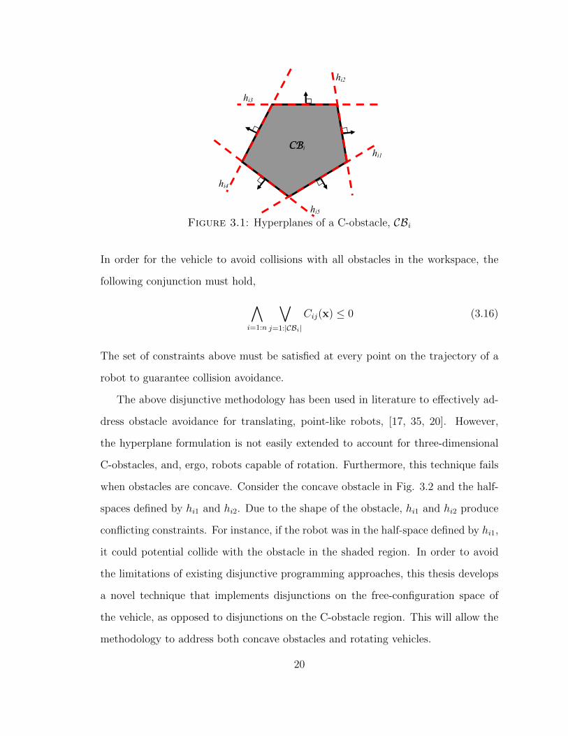
(x) 0 (3.16)

The set of constraints above must be satisfied at every point on the trajectory of a

robot to guarantee collision avoidance.

The above disjunctive methodology has been used in literature to e↵ectively ad-

dress obstacle avoidance for translating, point-like robots, [17, 35, 20]. However,

the hyperplane formulation is not easily extended to account for three-dimensional

C-obstacles, and, ergo, robots capable of rotation. Furthermore, this technique fails

when obstacles are concave. Consider the concave obstacle in Fig. 3.2 and the half-

spaces defined by h

i1 and h

i2. Due to the shape of the obstacle, hi1 and h

i2 produce

conflicting constraints. For instance, if the robot was in the half-space defined by h

i1,

it could potential collide with the obstacle in the shaded region. In order to avoid

the limitations of existing disjunctive programming approaches, this thesis develops

a novel technique that implements disjunctions on the free-configuration space of

the vehicle, as opposed to disjunctions on the C-obstacle region. This will allow the

methodology to address both concave obstacles and rotating vehicles.

20

CBi

hi2 hi1

Conflict Region 

Figure 3.2: Conflict Region for a Concave Obstacle

21

4

The Unicycle Model

This chapter presents a novel discretization of the vehicle kinematics in the form of a

piece-wise linear time invariant (PWLTI) system. Chapter 2 has shown that PWLTI

systems can be easily included in mixed integer programs (MIP). The technique below

constructs a set of linear mixed integer constraints that e↵ectively approximate the

nonlinear, time invariant system kinematics of the vehicle.

The maneuverability of the robot is defined by the unicycle kinematics. The state

of the robot is given by the position and orientation of the vehicle x = [x, y, ✓]T, and

the instantaneous linear and angular velocities of the vehicle constitute the control

vector, u = [v, !]T. Where both x and u are functions of time. In the unicycle

model, the time derivatives of the state variables cannot take independent values.

Rather, the state variables, their derivatives, and the control variables are related

through the following set of equations.

x = v cos ✓ (4.1)

y = v sin ✓ (4.2)

✓ = ! (4.3)

22

Formally, the statements above mathematically define the unicycle kinematics. This

model is commonly referred to as a kinematic relationship, as it does not address

the forces or torques on the robot, [36]. Using a vector notation, Eqn. 4.1 - 4.3 can

be written more concisely as

x =

2

4cos ✓ 0sin ✓ 00 1

3

5u (4.4)

Eqn. 4.4 is commonly referred to as the state equation.

In the unicycle model, the linear velocity of the vehicle is always along its main

axis. This condition can be expressed as follow

x sin ✓ � y cos ✓ = 0 (4.5)

In robotics literature, this relationship is referred to as the no-slip condition, [37].

Physically, this means that the vehicle can only move in the direction that its wheels

face. This assumption is a well established limitation of wheeled vehicles in moderate

speed scenarios, [38]. The no-slip condition is a nonholonomic constraint on the

system variables.

Definition 3. A nonholonomic constraint, [6], is a non-integrable equality con-

straint that is a function of the state variables of a system and their derivatives.

The controllability of vehicles with nonholonomic kinematics is investigated in

[39]. In summary, it was found that a robot governed by a single nonholonomic

equality constraint is fully controllable, [6]. A vehicle is fully controllable if it is able

to follow any collision free path in W . By these definitions, a robot with unicycle

kinematics is fully controllable.

23

4.1 Temporal Discretization

The trajectory problem must be discretized in time so that a numerical solution can

be computed. This research implements a first order, Euler discretization of the

continuous kinematics found in Eqn. 4.1 - 4.3, where �t and k are identical to those

defined in Chapter 2. The unicycle model in discrete time is given by

x

k+1 = x

k

+�t (vk

cos ✓k

) (4.6)

y

k+1 = y

k

+�t (vk

sin ✓k

) (4.7)

✓

k+1 = ✓

k

+�t !

k

(4.8)

Using vector notation the above equations can be written as

x

k+1 =

2

41 0 00 1 00 0 1

3

5x

k

+

2

4�t (cos ✓

k

) 0�t (sin ✓

k

) 00 �t

3

5u

k

(4.9)

The first-order Euler approximation is a useful and easily computed temporal

discretization, however, it is a temporally linear discretization and is therefore only

valid over short time intervals. Therefore, discretion must be used when selecting

the values for �t, N , and T for a particular system.

4.2 PWLTI Angular Discretization

The MIP optimization software used in this research, Tomlab/CPLEX, is most e↵ec-

tively utilized in problems where the mixed integer constraints are linear. Although

nonlinear programming packages are available, the computational requirements of

solutions for nonlinearly constrained MIPs are numerically demanding. The uni-

cycle model, even in discrete time, is nonlinear in ✓

k

due to the no-slip condition.

Therefore, it is necessary to approximate Eqn. 4.9 by a set of linear equations. This

is accomplished by use of the PWLTI framework described in Chapter 3.

24

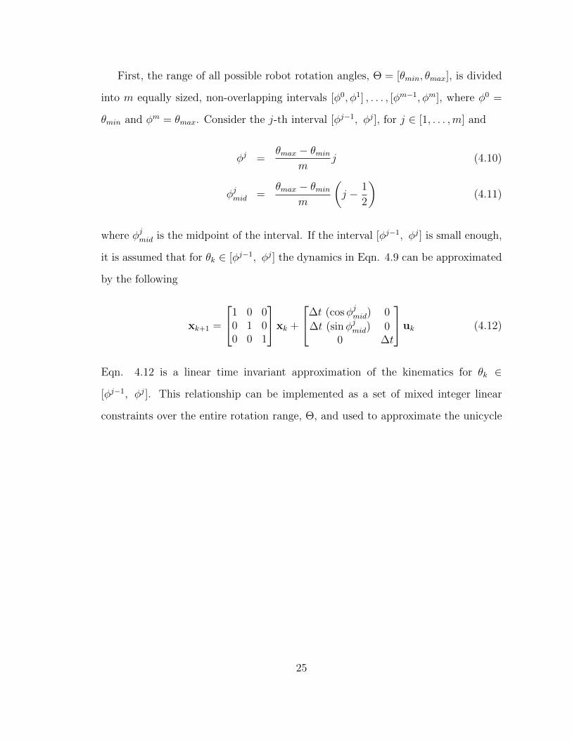
First, the range of all possible robot rotation angles, ⇥ = [✓min

, ✓

max

], is divided

into m equally sized, non-overlapping intervals [�0,�

1] , . . . , [�m�1,�

m], where �

0 =

✓

min

and �

m = ✓

max

. Consider the j-th interval [�j�1, �

j], for j 2 [1, . . . ,m] and

�

j =✓

max

� ✓

min

m

j (4.10)

�

j

mid

=✓

max

� ✓

min

m

✓j � 1

2

◆(4.11)

where �j

mid

is the midpoint of the interval. If the interval [�j�1, �

j] is small enough,

it is assumed that for ✓k

2 [�j�1, �

j] the dynamics in Eqn. 4.9 can be approximated

by the following

x

k+1 =

2

41 0 00 1 00 0 1

3

5x

k

+

2

4�t (cos�j

mid

) 0�t (sin�j

mid

) 00 �t

3

5u

k

(4.12)

Eqn. 4.12 is a linear time invariant approximation of the kinematics for ✓

k

2

[�j�1, �

j]. This relationship can be implemented as a set of mixed integer linear

constraints over the entire rotation range, ⇥, and used to approximate the unicycle

25

kinematics. The approximation of the kinematic model is as follows

8 j 2 [1, . . . ,m]

x

k+1 A

j

x

k

+B

j

u

k

+M(1� �

j

k

) (4.13)

x

k+1 � A

j

x

k

+B

j

u

k

�M(1� �

j

k

) (4.14)

A

j =

2

41 0 00 1 00 0 1

3

5 (4.15)

B

j =

2

4�t cos�j

mid

0�t sin�j

mid

00 �t

3

5 (4.16)

✓

k

�

j +M(1� �

j

k

) (4.17)

✓

k

� �

j�1 �M(1� �

j

k

) (4.18)

mX

j=1

�

j

k

= 1 (4.19)

These equations are in the form of the mixed integer representation of the general

PWLTI system. The discretization of the nonholonomic unicycle kinematics in the

form of a PWLTI system is a novel approach developed in this research for a rotating

robot.

26

5

Background on Approximate Cell Decomposition

Cell decomposition is a well established class of solution methods for robotic path

planning in obstacle populated environments. The primary step of these algorithms

is to decompose the free configuration space, Cfree

, into a set, Kvoid

, of empty (i.e.

conflict free), convex regions called cells. Cell decomposition methods are categorized

as either exact or approximate. In exact cell decomposition (ECD), the union of the

void cells is exactly the free configuration space of the robot, i.e. [Kvoid

= Cfree

.

ECD has been studied in detail as it is a complete planning method. However,

obtaining an ECD of a workspace is not always a computationally realistic procedure

as the complexity of obtaining such a decomposition grows drastically with workspace

dimension and size. As a result, ECD is commonly restricted to the set of problems

containing planar or convex polyhedral obstacles [40, 41, 42, 43], and vehicles capable

of translation only.

Approximate cell decomposition (ACD) algorithms result in a set of convex, non-

overlapping polygons of a predefined shape. In these methods, Kvoid

is a conservative

representation of the free space. Therefore, the union of cells in Kvoid

which form a

bounded approximation of the free configuration space, i.e. [Kvoid

✓ Cfree

. As is

27

the case with exact cell decomposition, ACD can be accomplished using a variety

of techniques. This research implements a quadtree approach to ACD, in which the

free configuration space is decomposed into cells with square projections on the x�y

plane, [44]. Alternative techniques, such as the approximate-and-decompose method,

[45], that decomposes Cfree

into rectangloid cells, have been successfully implemented

for similar motion planning problems, [14, 46, 15].

5.1 Quadtree Decomposition

Quadtrees are hierarchical data structures that are used to partition two-dimensional

spaces, [47]. They are frequently implemented as a way to approximately decompose

the void configuration space in obstacle populated environments, [44]. For each C-

obstacle space obtained by orientation slicing a decomposition was computed using

the quadtree approach, [6]. The algorithm work by recursively dividing the workspace

into cells and labeling these cells as FULL, EMPTY or MIXED. A cell is characterized

as FULL if its interior is completely contained in a C-obstacle, as EMPTY if its

interior intersects no C-obstacles, and as MIXED otherwise. The technique begins by

dividing the workspace into four quadrants, which are then labeled. If a cell is FULL

the algorithm does nothing. Cells labeled EMPTY are added to the set of void cells,

Kvoid

. If a cell is MIXED, it is divided into four equally sized quadrants, which are

then labeled and stored, ignored, or divided accordingly. The quadtree decomposition

recursively divides MIXED cells until a minimum cell size, or resolution, is reached.

When the algorithm terminates, the set of empty cells, Kvoid

, is returned.

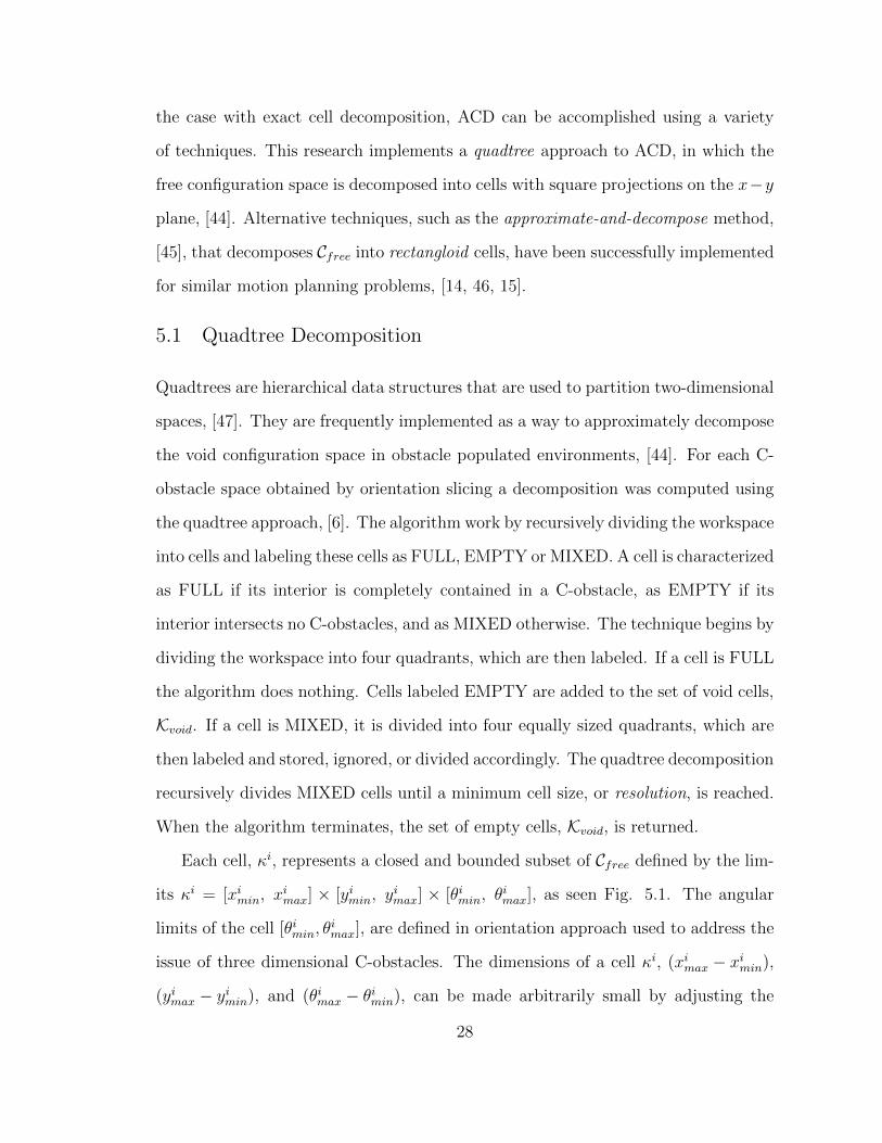
Each cell, i, represents a closed and bounded subset of Cfree

defined by the lim-

its

i = [xi

min

, x

i

max

] ⇥ [yimin

, y

i

max

] ⇥ [✓imin

, ✓

i

max

], as seen Fig. 5.1. The angular

limits of the cell [✓imin

, ✓

i

max

], are defined in orientation approach used to address the

issue of three dimensional C-obstacles. The dimensions of a cell i, (xi

max

� x

i

min

),

(yimax

� y

i

min

), and (✓imax

� ✓

i

min

), can be made arbitrarily small by adjusting the

28

resolution limits of the quadtree decomposition. However, applying finer resolutions

increases the running time of the path planning algorithm. Therefore, a trade o↵ ex-

ists between the precision of the approximation and the completeness of the solution.

As a result, ACD methods are often called resolution complete, [6].

x

y

θ

� �ii yy minmax �

Figure 5.1: Geometry of cell i

5.2 The Connectivity Graph

A primary assumption of the find path problem is that the robot moves continuously

through the workspace. In a decomposed environment it can be shown that the

assumption of a continuous path leads to the following claim: a robot is only capable

of moving from the cell containing its current orientation to the set of geometrically

adjacent cells or staying in its current cell. Let int(R1, R2) indicate the intersection

of the rectangles defined by R1 and R2. Adjacency is defined for two cells, i =

[xi

min

, x

i

max

] ⇥ [yimin

, y

i

max

] ⇥ [✓imin

, ✓

i

max

] and

j =⇥x

j

min

, x

j

max

⇤⇥⇥y

j

min

, y

j

max

⇤⇥

⇥✓

j

min

, ✓

j

max

⇤, if one of the following is true [14],

1. The int

�[xi

min

, x

i

max

]⇥ [yimin

, y

i

max

] ,⇥x

j

min

, x

j

max

⇤⇥⇥y

j

min

, y

j

max

⇤�projected

onto the x � y plane is greater than zero, and [✓imin

, ✓

i

max

] \⇥✓

j

min

, ✓

j

max

⇤6= ;,

Fig. 5.2(a).

29

θ

y

x

adjacent area in the x-y plane

(a)

θ

x

y

adjacent area in the y-θ plane

(b)

θ

x

y

adjacent area in the x-θ plane

(c)

Figure 5.2: Adjacency Relationships for Various Cell Orientations

2. The int

�[yi

min

, y

i

max

]⇥ [✓imin

, ✓

i

max

] ,⇥y

j

min

, y

j

max

⇤⇥⇥✓

j

min

, ✓

j

max

⇤�projected

onto the y � ✓ plane is greater than zero, and [xi

min

, x

i

max

] \⇥x

j

min

, x

j

max

⇤6= ;,

Fig. 5.2(b).

3. The int

�[xi

min

, x

i

max

]⇥ [✓imin

, ✓

i

max

] ,⇥x

j

min

, x

j

max

⇤⇥⇥✓

j

min

, ✓

j

max

⇤�projected

onto the x � ✓ plane is greater than zero, and [yimin

, y

i

max

] \⇥y

j

min

, y

j

max

⇤6= ;,

Fig. 5.2(c).

The adjacency relationships of a workspace can be defined concisely in a connectivity

graph.

Definition 4. A connectivity graph, G, is an undirected graph, where vertices

represent void cells and edges correspond to adjacency relationships of the cells. An

edge, (i

,

j), exists in G connecting vertices

i and

j if and only if the respective

30

cells are adjacent in Kvoid

, [14].

For pictorial simplicity, consider the two dimensional, decomposed workspace

found in Fig. 5.3. By application of the adjacency definitions above, the connectivity

graph for Fig. 5.3 was easily determined. It is found in Fig. 5.4.

κ13

κ12 κ11

κ10 κ9

κ8 κ7

κ6 κ5

κ4 κ3

κ2

κ1

Void cell

C-obstacle

Figure 5.3: Example - Decomposed Workspace, Kvoid

κ1

κ2

κ3 κ4

κ5

κ6

κ7 κ8

κ9 κ10

κ11 κ12

κ13

Figure 5.4: Example: Connectivity Graph, G

31

In classical path planning algorithms that implement ACD, the solution method

is four-fold. First, the workspace is decomposed into a set of collision-free cells, Kvoid

,

using some form of ACD. Then the adjacency relationships are used to construct the

connectivity graph, G, of the workspace. The connectivity graph is then searched for

a sequence of cells connecting the

init, the cell containing the initial configuration,

and

final, the cell containing the goal configuration. These sequences of void cells

are referred to as channels. Finally, when a void channel between

init and

final

is found (using a graph searching technique) the path planning method concludes

by determining a feasible path within the channel. The research presented in this

thesis does not search the connectivity graph directly, rather, it transforms G into a

directed graph called the connectivity tree, as outlined in Chapter 6.

32

6

The Connectivity Tree

Many methods have been devloped to search connectivity graphs for channels con-

taining distance optimal collision free paths. This research implements a connectivity

tree approach, similar to that outlined in [14] and [13]. In these articles, the authors

use tree graphs to reduce the number of channels explored between

init 3 x0 and

final 3 x

N

.

Definition 5. A connectivity tree, T , is a tree graph associated with G, where

init is the root and

final is in the leaves of the tree. A connected path from the root

to a leaf is referred to as a branch and represents a channel in Kvoid

connecting init

to

final.

Unfortunately, the span of a connectivity tree grows dramatically with its depth.

In order to avoid the computational complexity associated with a large connectivity

tree a pruning algorithm can be used to remove suboptimal, redundant and super-

fluous paths from T , [14]. A pruning algorithm algorithm assigns a weight to each

edge in T , and removes suboptimal paths by application of the Bellman equation of

optimality, [31].

33

Many pruning techniques are unable to consider kinematic feasibility in branch re-

moval. Consequently, the robot is often unable to e↵ectively traverse the workspace.

The following section presents an initial methodology for retaining a larger number

of kinematically feasible paths. Importantly, the pruning algorithm used was created

so that the techniques developed in this research could be tested. At this stage of

the investigation, no current claims have been made regarding the optimality of this

pruning technique. However, future work on the pruning algorithm aims to address

optimality and completeness concerns.

6.1 Entry Nodes and the Connectivity Tree

This approach introduces the concept of entry nodes. An entry node, ⌘ij

, is a repre-

sentative point for the adjacency relationship of two cells, i and

j. The position of

the node is selected such that it corresponds to the geometric center of the adjacent

area of i and

j. The node ⌘

ij

is used as an approximation of the location that a

robot would pass through if it was to enter

j from

i; and, as expected, ⌘ij

= ⌘

ji

.

For simplicity, once again, consider the decomposed workspace found in Fig. 5.3,

and the corresponding connectivity graph, G, in Fig. 5.4. Once a connectivity graph

has been obtained for a workspace, determining the positions of the entry nodes

is trivial. Then, the connectivity of the entry nodes must be determined. Entry

nodes are connected in Kvoid

if they are positioned on the boundary of the same cell.

These relationships create a new connectivity graph, G⌘, for the entry nodes of the

workspace as opposed to the cells. The node connectivity of the example workspace

is shown in Fig. 6.1. An additional node is added to G⌘ corresponding to the initial

configuration of the robot, and, as seen in Fig. 6.1, it is connected to the entry nodes

associated with

init. Furthermore, the connectivity of the entry nodes of final are

not included.

In this newly created connectivity graph, G⌘, the arcs are assigned weights corre-

34

node for initial orientation cell entry node entry node for cell containing final orientation node connectivity

Figure 6.1: Example - Entry Node Connectivity, G⌘

sponding to the Euclidean distance between the nodes. Dijkstra’s algorithm, [48, 49],

can then be used to find optimal sequences of nodes, based on the associated connec-

tivity weights, between the node corresponding to the initial configuration and the

entry nodes of the final cell. Alternative graph searching methods to Dijkstra’s algo-

rithms, such as dynamic programming are available, however, as previously stated,

the pruning algorithm is not the focus of this. Later work will investigate the variety

of graphical methods available. The optimized connectivity graph, G⌘

opt

, for the nodes

in Fig. 6.1 is shown in Fig. 6.2. The graph, G⌘

opt

, is then mapped back to the original

void cells. This mapping leads to a pruned connectivity tree, T , that will be used

in determining the optimal trajectory. The final connectivity tree of the example

workspace can be found in Fig. 6.3. This methodology is easily extended to account

for a three dimensional decomposition. Fig. 6.4 shows a possible sequence of entry

node connected in a three dimensional space. The branches of T will be included as

constraints in the final MIQP, as explained in the following section. From this point

35

forward, references to the connectivity tree or T will regard the pruned tree.

node for initial orientation cell entry node entry node for cell containing final orientation node connectivity

Figure 6.2: Example - Optimal Entry Node Connectivity, G⌘

opt

κ1 κ3 κ4 κ5

κ8

κ9

κ10 κ11 κ12

κ12

Figure 6.3: Example - Pruned Connectivity Tree, T

6.2 Mixed Integer Representation of the Connectivity Tree

If the configuration of the robot at time step k is contained by any cell,

i =

[xi

min

, x

i

max

] ⇥ [yimin

, y

i

max

] ⇥ [✓imin

, ✓

i

max

], i.e.

i 3 x

k

, the robot will not collide

36

y

θ

x

Figure 6.4: Example - Node Connectivity in Three Dimensions

with the obstacles. This condition is analogous to the following set of constraints

x

i

min

x

k

x

i

max

y

i

min

y

k

y

i

max

✓

i

min

✓

k

✓

i

max

(6.1)

Consider a branch, b`

, in T , where ` 2 [1, . . . , s] and s is the total number of branches.

By definition, b`

corresponds to an ordering of cells from

init to

final. Let ⇤[b`

]

denote the length in cells of branch b

`

. If the robot is capable of following a kinemat-

ically feasible path in b

`

, it will avoid collisions with all obstacles along its trajectory.

All cells in b

`

, i = b

`

[i] 8i 2 [1, . . . ,⇤(b`

)], do not need to be considered as probable

locations of the vehicle for all time steps k. In order to decrease the number of

constraints at each time step, time allocations must be defined for each cell.

By inspection, the most time consuming path (without backtracking) through

a cell i is associated with entering through one corner, i.e. (xi

min

, y

i

min

), with

orientation angle ✓

i

min

and exiting the cell at the diagonally opposite corner, i.e.

(xi

max

, y

i

max

), with orientation angle ✓

i

max

. The goal is to determine the number of

discrete time steps required to traverse i. This research proposed that the maximum

number of time steps, �k, necessary to enter and exit i can be found by calculating

the time requirement of an arc, ↵, across the cell, see Fig. 6.5. Consider a cell from

37

the quadtree ACD that has a square projection on the x�y plane, i.e. (xi

max

�x

i

min

) =

(yimax

�y

i

min

). Let �x

i = (xi

max

�x

i

min

), �y

i = (yimax

�y

i

min

) and �✓

i = (✓imax

�✓

i

min

);

the length of the arc can be approximated as

↵ =d

2

�✓

i

sin (�✓

i

/2)(6.2)

Where, by simple cell geometry,

d =p2�x

i (6.3)

The continuous time, t↵

, to traverse the arc ↵ is as follows

t

↵

=↵

v

avg

(6.4)

where v

avg

is an approximation of the velocity of the vehicle. In this research, vavg

was set to 75 % of the maximum allowable velocity, vmax

. Using the above equations,

�k can be determined by

�k =

⇠t

↵

�t

⇡

=

& p2�x

i�✓

i

v

avg

�t

!1

sin(�✓

i

/2)

'(6.5)

The value of �k can be easily calculated for the varying cell dimensions of Kvoid

.

The number of discrete time steps for a particular cell i will be denoted as �k[i].

Once again consider a branch, b`

, of the connectivity tree T . By applying the

�k-rule defined in Eqn. 6.5, the constraints requiring that a vehicle remain in the

channel defined by b

`

can be approximated as

k

count

= 0

for i = 1 : ⇤(b`

) do

i = b

`

[i]

38

d

α

Δ xi

θimax

Δ yi

y

θimin

x

Figure 6.5: Determining �k for a cell, i

for k = k

count

: (kcount

+�k[i]) do

x

i

min

x

k

x

i

max

y

i

min

y

k

y

i

max

✓

i

min

✓

k

✓

i

max

end for

k

count

= k

count

+�k[i] + 1

end for

A robot is only able to travel along a single channel between

init and

final.

Consequently, only the constraints of one branch can be true along the optimal

path. This condition can be addressed by introducing binary decision variables, �`

,

for each branch, b`

, as follows

for ` = 1 : s do

k

count

= 0

for i = 1 : ⇤(b`

) do

i = b

`

(i)

for k = k

count

: (kcount

+�k[i]) do

x

k

x

i

max

+M(1� �

`

)

x

k

� x

i

min

�M(1� �

`

)

39

y

k

y

i

max

+M(1� �

`

)

y

k

� y

i

min

�M(1� �

`

)

✓

k

✓

i

max

+M(1� �

`

)

✓

k

� ✓

i

min

�M(1� �

`

)

end for

k

count

= k

count

+�k[i] + 1

end for

end for

sX

`=1

�

`

= 1

In the equations above big M theory has been used to address disjunctions between

the branches. The final constraint in the statements above guarantees that only one

branch of the tree is applied in the final trajectory calculation.

40

7

MIQP for Collision-Free Path Planning

Chapter 4 describes the procedure developed by this thesis to discretize the continu-

ous, nonholonomic unicycle kinematics of the robot into a set of linear mixed integer

constraints. These conditions, as well those defined for the free configuration space

in Chapter 6, are included in the final optimization algorithm below. In order to

provide a more realistic vehicle model, constraints on the maximum and minimum

linear and angular velocities are introduced. These conditions are defined in the

following section.

7.1 Velocity Constraints and Initial and Final Conditions

Additional constraints to those defined in Chapter 4 and Chapter 6 are required in the

final mixed integer quadratic program (MIQP) to completely and realistically model

a wheeled vehicle. In most motion planning scenarios the linear and angular velocities

are each bounded by some maximum value as result of the physical limitations of

the vehicle. For the discrete linear and angular velocities, with maximums vmax

and

41

!

max

, respectively, the constraints are as follows

|vk

| v

max

(7.1)

|!k

| !

max

(7.2)

The above equations can be expressed by the linear constraints below

�v

max

v

k

v

max

(7.3)

�!

max

!

k

!

max

(7.4)

As stated in Chapter 2, the vehicle must begin in a prescribed initial configura-

tion, xinit

. This condition is given by, where x(t = 0) = x0

x0 = x

init

(7.5)

Similarly, for the final (or goal) configuration, where x(t = T ) = x

N

x

N

= x

final

(7.6)

If the robot arrives at xfinal

before step N , i.e. xk

= x

final

for k < N , no additional

cost is acquired based on the formulation of the optimization function, Eqn. 2.12.

7.2 Methodology Summary

Given a workspace W , populated by n stationary, polygonal obstacles, a robot A

with unicycle kinematics, and initial and goal configurations xinit

and x

final

, the tra-

jectory planning optimization is as follows. Begin by obtaining an approximate cell

decomposition of the configuration space, Kvoid

, via the quadtree approach. Then,

using the adjacency relationships of the cells, construct a connectivity graph, G, of

the workspace. This graph is then used to determine the connectivity of the entry

nodes of the cells, G⌘. Using Dijkstra’s algorithm prune G⌘ for optimal sequences of

nodes between the initial node and the entry nodes of the final cell. These sequences

42

Discretize

kinematics in

time

xinit, xfinal, J(x),

Θ, W, A

Discretize

kinematics in

θ

Calculate

C-obstacle for

θ intervals

Determine the

connectivity

graph

ACD via

Quadtree

method

Determine

entry node

connectivity

Apply Pruning

Algorithm

x(t)

CB Kvoid G

Gη

xk Mixed integer

representation

of kinematics

Mixed integer

representation

of branches

CPLEX

resolution

Orientation

slicing

Δt, T, N m

Final

Trajectory

T

Figure 7.1: Summary of Methodology

will be mapped back to their corresponding cells, resulting in a pruned connectivity

tree, T .

At this point, the optimization over the L2 norm of the state variables can be

solved using MATLAB [50], and the Tomlab/CPLEX [51, 32] interface for MIQP.

The final MIQP includes the discretized unicycle model (Chapter 4), the branch

containment conditions (Chapter 6) and the set of additional constraints defined

above. The complete optimization problem is defined below and summarized in Fig.

7.1.

minx

J(x) =NX

k=1

(xk

� x

k�1)T(x

k

� x

k�1)

Subject to:

x0 = x

init

x

N

= x

final

for k = 0 : N � 1 do

43

�v

max

v

k

v

max

�!

max

!

k

!

max

for j = 1 : m do

A

j =

2

41 0 00 1 00 0 1

3

5

B

j =

2

4�t cos�j

mid

0�t sin�j

mid

00 �t

3

5

x

k+1 A

j

x

k

+B

j

u

k

+M(1� �

j

k

)

x

k+1 � A

j

x

k

+B

j

u

k

�M(1� �

j

k

)

✓

k

�

j +M(1� �

j

k

)

✓

k

� �

j�1 �M(1� �

j

k

)

�

j

k

= 0 or 1

end for

mX

j=1

�

j

k

= 1

end for

for ` = 1 : s do

k

count

= 0

for i = 1 : ⇤(b`

) do

i = b

`

(i)

for k = k

count

: (kcount

+�k[i]) do

x

k

x

i

max

+M(1� �

`

)

x

k

� x

i

min

�M(1� �

`

)

y

k

y

i

max

+M(1� �

`

)

y

k

� y

i

min

�M(1� �

`

)

✓

k

✓

i

max

+M(1� �

`

)

44

✓

k

� ✓

i

min

�M(1� �

`

)

end for

k

count

= k

count

+�k[i] + 1

end for

�

`

= 0 or 1

end for

sX

`=1

�

`

= 1

The following chapter documents the results obtained for various workspaces using

the methodology defined above.

45

8

Results

This chapter presents a handful of trajectory simulations obtained via the method-

ology developed in this thesis. The algorithm was implemented in CPLEX, [32],

a commercially available optimization software, using a Tomlab, [51], interface for

MATLAB, [50]. The following values were used in the path simulations of a 1 unit

by 2 unit rectangular robot: �t = 0.75 s, vmax

= 5 units/s, !max

= 0.20 rad/s,

�✓ = ⇡/6 rad (✓ discretization of all cells), and m = 21 (discretization of the kine-

matics). From here on, A will indicate the initial configuration of the vehicle in the

pictorial results.

8.1 Kinematic Trajectory Planning

Before addressing obstacle avoidance concerns, the kinematic constraints developed

by this research, see Chapter 4, were tested. Fig. 8.1 shows the optimization of the

discretized cost function for a robot with initial configuration x

init

= [4, 4, 0]T and

final configuration x

final

= [4, 6, ⇡]T. The trajectory returned for this scenario shows

that the PWLTI representation of the vehicle maneuverability is an e↵ective and

useful discretization of the unicycle kinematics. An important consideration to take

46

into account when analyzing the paths of unicycle-like robots is that v(t) = 0, and

consequently, vk

= 0, are admissible control inputs for the continuous and discrete

linear velocities, respectively. Physically, this means that the robot is capable of

rotating in ⇥ while remaining stationary in W , i.e. rotating in place. As this is

generally not the case for real vehicles, many models impose constraints on the

turning radius or steering angle of the robot, [38]. However, as this is an initial stage

of research, this thesis allowed the robot to rotate without translation, as is typical

of the unicycle model. Fig. 8.2 documents a similar path, but over a longer distance

where x

final

= [4, 10, ⇡]T.

x

y

A

Figure 8.1: Kinematics - Path A

The numerical simulations shown in Fig. 8.3 and Fig. 8.4 depict the importance

of the orientation angle of the vehicle in ⇥. In both scenarios, the vehicle begins in

state x

init

= [4, 4, 0]T and ends with the centroid of the platform at (x, y) = (12, 6).

In Fig. 8.3 the robot begins and ends with orientation angle at 0 rad, resulting in

a relatively simple trajectory between the initial and final states. Fig. 8.4, on the

47

x

y

A

Figure 8.2: Kinematics - Path B

other hand, exhibits a more complicated path. In this case the vehicle begins at 0 rad

and ends facing the opposite direction at ⇡ rad. The importance of this simulation

is that given certain conditions traveling in reverse results may result in the optimal

path, as is the case in many real world problems.

The results found in Fig. 8.1 - 8.4 show various paths obtained via the PWLTI

representation of the vehicle kinematics. These simulations exhibit that the method-

ology developed can e↵ectively discretize the nonholonomic relationships of the uni-

cycle model and retain the original maneuverability.

8.2 Workspace 1

Following the verification of the vehicle kinematics, the connectivity tree method-

ology was tested as a means of obstacle avoidance for a simple workspace. The

workspace was decomposed using the quadtree technique with a minimum resolu-

tion of 0.5 units. Fig. 8.5 demonstrates the maneuverability of a robot in a two

48

x

y

A

Figure 8.3: Kinematics - Path C

x

y

A

Figure 8.4: Kinematics - Path D

49

y

A

x

Figure 8.5: Workspace 1

dimensional workspace containing a single convex obstacle. The path arrived at in

this workspaces exhibits the ability of the methodology developed in this thesis to

address obstacle avoidance simultaneously with kinematic considerations.

8.3 The Parking Garage Problem

The following simulations require a robot to “park” in di↵erent workspace “garages”

which are modeled as concave obstacles. The results obtained show that the robot

is able to traverse small channels in concave environments, a limitation of other

techniques. This is a marked improvement on previous disjunctive programming

(DP) methodologies, which were unable to address concave workspaces, as shown in

Chapter 3.3. Both Fig. 8.6 and Fig. 8.7 show simulations for two di↵erent, successful

parking maneuvers in the workspace.

The environment found in Fig. 8.8, and the initial and final configurations of

50

y

A

x

Figure 8.6: Parking Garage - Path A

y

A

x

Figure 8.7: Parking Garage - Path B

51

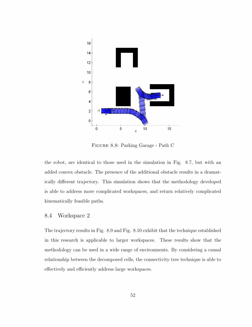
y

A

x

Figure 8.8: Parking Garage - Path C

the robot, are identical to those used in the simulation in Fig. 8.7, but with an

added convex obstacle. The presence of the additional obstacle results in a dramat-

ically di↵erent trajectory. This simulation shows that the methodology developed

is able to address more complicated workspaces, and return relatively complicated

kinematically feasible paths.

8.4 Workspace 2

The trajectory results in Fig. 8.9 and Fig. 8.10 exhibit that the technique established

in this research is applicable to larger workspaces. These results show that the

methodology can be used in a wide range of environments. By considering a causal

relationship between the decomposed cells, the connectivity tree technique is able to

e↵ectively and e�ciently address large workspaces.

52

y

A

x

Figure 8.9: Workspace 2 - Path A

y

A

x

Figure 8.10: Workspace 2 - Path B

53

9

Conclusions

Due to the growing need for autonomous systems in both military and civilian ap-

plications, a large amount of research e↵ort has been focused on the class of robotic

motion planning problems. This class of problems has been used in a variety of appli-

cations ranging from mine-detection to mobile router connectivity, [18]. The research

discussed in this thesis concentrated on one of the fundamental paradigms of trajec-

tory planning, the find-path problem. In this benchmark problem, the robot must

navigate an obstacle populated environment while avoiding collisions with stationary

obstacles, the positions and geometries of which are assumed known a priori. This

paradigm is well researched in the robotics community, and, as a result, a plethora

of solution methods has been developed. The focus of this research was on the cell

decomposition and the mathematical programming classes of motion planners. Both

of these methods have been shown to be complete, or, at least, resolution complete

planning algorithms, and are also considered to be global methodologies, [6].

Cell decomposition methodologies are able to e↵ectively address obstacle avoid-

ance concerns, [14], however many of these techniques are not readily extended to

solve for optimal control problems in a manner that would be able to guarantee opti-

54

mality. Cell decomposition of workspaces are both time and memory demanding, as

the volume of the decomposition grows exponentially with the degrees of freedom of

the vehicle. Mixed integer programming (MIP) is a mathematical programming tech-

niques that has been successfully implemented for optimal control problems. These

methods are complete and are accomplished directly in the workspace, rather than

a higher dimensional space, such as the configuration space. An added benefit is

that MIP techniques are readily applied to convex obstacle avoidance, without any

preprocessing of the workspace. MIP methods are revered for their flexibility and

ability to address a variety of optimal control problems, while guaranteeing optimal-

ity. However, these techniques su↵er from a handful of restrictions. For one, they

are not readily applicable to concave obstacles or rotating vehicles. Furthermore,

the computation requirements of solving MIP grow drastically with the number of

binary variables.

This these proposes a combination of MIP and cell decomposition. Results show

that the method is able to address many of the concerns of both MIP and cell

decomposition techniques. In particular, the methodology is able to handle concave

obstacles, rotating vehicles, and the optimal control problem. Furthermore, this

research presents a novel discretization of the nonholonomic unicycle model in the

form of a piece-wise linear time invariant system, resulting in a set of mixed integer

constraints that can be easily included in a final optimization problem.

9.1 Summary of Results

The simulations depicted in Chapter 8 show the e↵ectiveness of the methodology

in addressing obstacle avoidance in a variety of di↵erent workspaces while simul-

taneously considering kinematic constraints. This thesis extends previous work in

mixed integer programming for motion planning, which modeled vehicles as free-

flying robots without geometries, to scenarios including vehicle geometries, rotation,

55

and kinematic considerations. The PWLTI approach proves to be an e�cient and

easily implemented approximation of the nonholonomic unicycle model.

By use of the entry node pruning algorithm defined in Chapter 6, the methodology

was able to retain multiple channels in which a kinematically feasible path could

exist. Although results can be obtained using the pruning algorithm defined, further

research is needed to better address the dichotomy of optimal control and geometric

planning problems. This methodology assigned weights to the connectivity tree using

purely geometric considerations. Future research will examine alternative methods

for pruning including alternative weighting metrics and di↵erent definitions of nodes

in the workspace. In addition, this work will investigate kinematic considerations in

tree branches, similar to the work found in [28, 29, 52]. Furthermore, the pruning

algorithm in its current form is not able to claim completeness or optimality. Proofs

regarding these important characteristics, as well as a complexity analysis, must be

accomplished in order to determine the viability of the technique developed in this

thesis.

9.2 Future Work

This research considered the simple trajectory planning problem of a single robot in

an obstacle populated environment. Using the same paradigm, alternative kinematic

and dynamic constraints can be explored using the mixed-integer framework. Aside

from maneuverability considerations, a variety of other problems can be considered.

These include stationary and dynamic target detecting [15, 53], sensor planning and

control [54], and iterative applications of MIPs. Although a number of possible

directions exist for future research, the first step will be in determining a pruning

algorithm that takes into account kinematic considerations, and which can guarantee

solution optimality.

56

Bibliography

[1] Y. K. Hwang and N. Ahuja, “Gross motion planning: a survey,” ACM Comput.Surv., vol. 24, no. 3, pp. 219–291, Sep. 1992.

[2] M. H. Overmars and P. Svestka, “A probabilistic learning approach to motionplanning,” Utrecht University, Netherlands, Scientific Report, jan 1994.

[3] J. Barraquand and J.-C. Latombe, “Robot motion planning: a distributed rep-resentation approach,” Int. J. Rob. Res., vol. 10, no. 6, pp. 628–649, Dec. 1991.

[4] J. Barraquand, B. Langlois, and J.-C. Latombe, “Numerical potential field tech-niques for robot path planning,” Systems, Man and Cybernetics, IEEE Trans-actions on, vol. 22, no. 2, pp. 224 –241, 1992.

[5] J. Barraquand and J.-C. Latombe, “On nonholonomic mobile robots and op-timal maneuvering,” in Intelligent Control, 1989. Proceedings., IEEE Interna-tional Symposium on, sep 1989, pp. 340 –347.

[6] J. C. Latombe, Robot Motion Planning. Kluwer Academic Publishers, 1991.

[7] Y. Koren and J. Borenstein, “Potential field methods and their inherent limi-tations for mobile robot navigation,” in Robotics and Automation, 1991. Pro-ceedings., 1991 IEEE International Conference on, vol. 2, Apr 1991, pp. 1398–1404.

[8] B. Donald, P. Xavier, J. Canny, and J. Reif, “Kinodynamic motion planning,”Association of Computing Machinery, vol. 40, no. 5, pp. 1048–1066, 1993.

[9] J. van den Berg and M. Overmars, “Kinodynamic motion planning on roadmapsin dynamic environments,” in Intelligent Robots and Systems, 2007. IROS 2007.IEEE/RSJ International Conference on, 2007, pp. 4253 –4258.

[10] S. M. LaValle, M. S. Branicky, and S. R. Lindermann, “On the relationshipbetween classical grid search and probabilistic roadmaps,” International Journalof Robotics Research, 2004.

57

[11] S. M. LaValle and J. J. K. Jr., “Randomized kinodynamic planning,” Interna-tional Journal of Robotics Research, vol. 20, no. 5, pp. 378–400, 2001.

[12] D. Hsu, R. Kindel, J.-C. Latombe, and S. Rock, “Randomized kinodynamicmotion planning with moving obstacles,” 2000.

[13] S. Ferrari and C. Cai, “Information-driven search strategies in the board game ofclue,” Systems, Man, and Cybernetics, Part B: Cybernetics, IEEE Transactionson, vol. 39, no. 3, pp. 607 –625, June 2009.

[14] C. Cai and S. Ferrari, “Information-driven sensor path planning by approximatecell decomposition,” Trans. Sys. Man Cyber. Part B, vol. 39, no. 3, pp. 672–689,2009.

[15] S. Ferrari, R. Fierro, B. Perteet, C. Cai, and K. Baumgartner, “A geometricoptimization approach to detecting and intercepting dynamic targets using amobile sensor network,” SIAM J. Control Optim., vol. 48, no. 1, pp. 292–320,2009.

[16] L. Blackmore and B. Williams, “Optimal manipulator path planning with ob-stacles using disjunctive programming,” in American Control Conference, 2006.

[17] T. Schouwenaars, B. D. Moor, J. How, and E. Feron, “Mixed integer program-ming for multi-vehicle path planning,” in Proceedings of the European ControlConference, 2001, pp. 2603–2608.

[18] N. Bezzo, R. Fierro, A. Swingler, and S. Ferrari, “A disjunctive programmingapproach for motion planning of mobile router networks,” International Journalof Robotics and Automation, vol. 3, pp. 227–252, 2010.

[19] N. K. Yilmaz, C. Evangelinos, P. F. J. Lermusiaux, and N. M. Patrikalakis,“Path planning of autonomous underwater vehicles for adaptive sampling us-ing mixed integer linear programming,” IEEE Journal of Oceanic Engineering,vol. 33, no. 4, pp. 522–537, 2008.

[20] A. Richards, J. How, T. Schouwenaars, , and E. Feron, “Plume avoidance ma-neuver planning using mixed integer linear programming,” in Proceedings ofAIAA Guidance Navigation and Control Conference, 2001.

[21] A. Richards, T. Schouwenaars, J. How, and E. Feron, “Spacecraft trajectoryplanning with avoidance constraints using mixed-integer linear programming,”Journal of Guidance, Control, and Dynamics, vol. 25, no. 4, pp. 755–764, 2002.

58

[22] L. Pallottino, E. Feron, and A. Bicchi, “Conflict resolution problems for airtra�c management systems solved with mixed integer programming,” vol. 3,no. 1, 2002.

[23] R. Fierro and K. Wesselowski, “Optimization-based control of multi-vehicle sys-tems,” in Cooperative Control, ser. Lecture Notes in Control and InformationSciences, V. Kumar, N. Leonard, and A. Morse, Eds., 2005, vol. 309, pp. 461–463.

[24] A. Richards, Y. Kuwata, and J. How, “Experimental demonstrations of real-time milp control,” in In Proceeding of the AIAA Guidance, Navigation, andControl Conference, 2003.

[25] H. Ding, M. Zhou, and O. Stursberg, “Optimal path planning in the workspacefor articulated robots using mixed integer programming,” in Intelligent Robotsand Systems, 2009. IROS 2009. IEEE/RSJ International Conference on, oct.2009, pp. 5770 –5775.

[26] T. Schouwenaars, J. How, and E. Feron, “Receding horizon path planning withimplicit safety guarantees,” in Proceedings of the American Control Conference,2004, pp. 5576–5581.

[27] M. G. Earl and R. D’Andrea, “Iterative milp methods for vehicle-control prob-lems,” IEEE Transactions on Robotics, vol. 21, no. 6, pp. 1158 –1167, 2005.

[28] R. Cowlagi and P. Tsiotras, “On the existence and synthesis of curvature-bounded paths inside nonuniform rectangular channels,” in American ControlConference (ACC), 2010, 2010, pp. 5382 –5387.

[29] ——, “Kinematic feasibility guarantees in geometric path planning usinghistory-based transition costs over cell decompositions,” in American ControlConference (ACC), 2010, 2010.

[30] R. A. Brooks and T. Lozano-Perez, “A subdivision algorithm in configurationspace for findpath with rotation,” in Proceedings of the Eighth InternationalJoint Conference on Artificial Intelligence, 1983, pp. 799–806.

[31] D. E. Kirk, Optimal Control Theory: An Introduction. Prentice-Hall Inc., 1970.

[32] ILOG CPLEX 9.0 User’s Manual, ILOG, 2003.

[33] A. Bemporad and M. Morari, “Control of systems integrating logic, dynamics,and constraints,” Automatica, vol. 35, pp. 407–427, 1998.

59

[34] A. Bemporad, G. Ferrari-Trecate, and M. Morari, “Observability and controlla-bility of piecewise a�ne and hybrid systems,” IEEE Transactions on AutomaticControl, vol. 45, pp. 1864–1876, 2000.

[35] A. Richards and J. P. How, “Aircraft trajectory planning with collision avoid-ance using mixed integer linear programming,” in Proceedings of the AmericanControls Conference, 2002, pp. 1936–1941.

[36] P. Morin and C. Samson, Motion Control of Wheeled Mobile Robots, 2008, pp.779–826.

[37] A. D. Luca, G. Oriolo, and C. Samson, Robot Motion Planning and Control:Lectures Notes in Control and Information Sciences 229. Springer, ch. FeedbackControl of a Nonholonomic Car-Like Robot, pp. 170–253.

[38] D. Anisi, “Optimal motion control of a ground vehicle,” Swedish Defense Re-search Agency, Stockholm, Sweden, Scientific Report, July 2003.

[39] J. Barraquand and J. C. Latombe, “Controllability of mobile robots with kine-matic constraints,” Stanford University, Stanford, CA, Research, June 1990.

[40] K. Kedem and M. Sharir, “An e�cient algorithm for planning collision-freetranslational motion of a convex polygonal object in 2-dimensional space amidstpolygonal obstacles,” in Proceedings of the First Annual Symposium on Com-putational geometry, ser. SCG ’85. New York: ACM, 1985, pp. 75–80.

[41] F. Avnaim, J. Boissonnat, and B. Faverjon, “A practical exact motion planningalgorithm for polygonal objects amidst polygonal obstacles,” in Proceedings ofthe International Conference on Robotics and Automation, vol. 3, April 1988,pp. 1656 –1663.

[42] J. Schwartz and M. Sharir, “On the ‘piano movers’ problem: Ii. general tech-niques for computing topological properties of real algebraic manifolds,” Ad-vances in Applied Mathematics, vol. 4, pp. 298–351, 1983.

[43] K. Kedem and M. Sharir, “An e�cient motion planning algorithm for a convexpolygonal object in 2-dimensional polygonal space,” New York University, NewYork, Robotics Report 90, October 1986.

[44] N. I. Katevas, S. G. Tzafestas, and C. G. Pnevmatikatos, “The approximate celldecomposition with local node refinement global path planning method: Pathnodes refinement and curve parametric interpolation,” J. Intell. Robotics Syst.,vol. 22, no. 3-4, pp. 289–314, 1998.

60

[45] D. Zhu and J. C. Latombe, “New heuristic algorithm for e�cient hierarchicalpath planning,” IEEE Transactions on Robotics and Automation, vol. 7, no. 1,pp. 9–19, 1991.

[46] A. Swingler and S. Ferrari, “A cell decomposition approach to cooperative pathplanning and collision avoidance via disjunctive programming,” in Proc. of IEEEConf. Decision and Control, Atlanta, GA, 2010, pp. 6329–6336.

[47] H. Samet, “The quadtree and related hierarchical data structures,” ACM Com-put. Surv., vol. 16, no. 2, pp. 187–260, Jun. 1984.

[48] S. M. LaValle, Planning Algorithms. Cambridge University Press, 2006.

[49] D. Gleich, “gaimc: Graph algorithms in matlab code,” May 2009. [Online].Available: https://github.com/dgleich/gaimc

[50] MathWorks, “Matlab r2011a.” [Online]. Available: http://www.mathworks.com/products/matlab/

[51] K. Holmstrom, A. Goran, and M. Edvall, User’s Guide for Tomlab 7,TOMLAB OPTIMIZATION, 2009. [Online]. Available: http://tomopt.com/docs/TOMLAB.pdf

[52] A. Scheuer and T. Fraichard, “Continuous-curvature path planning for car-likevehicles,” in Intelligent Robots and Systems, 1997. IROS ’97., Proceedings of the1997 IEEE/RSJ International Conference on, vol. 2, Sep 1997, pp. 997 –1003.

[53] W. Lu, G. Zhang, and S. Ferrari, “A comparison of information theoretic func-tions for tracking maneuvering targets.”

[54] G. Zhang, W. Lu, and S. Ferrari, “An information potential approach to inte-grated sensor planning and control.”

61