Traitement de signal Analyse spectrale : Fourier, temps...
75
Traitement de signal Analyse spectrale : Fourier, temps-fr´ equence, temps-´ echelle Laurent Duval IFP Energies nouvelles, Rueil-Malmaison, France [email protected] September 23, 2015 1/60
-
Upload
nguyenxuyen -
Category
Documents
-
view
216 -
download
1
Transcript of Traitement de signal Analyse spectrale : Fourier, temps...
Traitement de signalAnalyse spectrale : Fourier,
temps-frequence, temps-echelle
Laurent Duval
IFP Energies nouvelles, Rueil-Malmaison, [email protected]
September 23, 2015
1/60

Motivation
• Standard framework• diversity and quantity of available data
• wide audience audio, image and video (main drive);exponentially increasing digital measures from different sensors(industrial, mobile devices)
• seismic data (petabytes)
• efficiency of standard (multi-dimensional) signal processingtechniques
• data acquisition and processing generally performed viastandard approaches (Nyquist-Shannon sampling, Fourieranalysis, parametric modeling, etc.), astonishingly efficient formost applications if properly used
2/60

Motivation
• Present challenges• ”Infobesity” : managing huge data volumes (information
overload amplified by explosion in precision and sampling ofdigital data ”made” cheaper by sensors and storage)
• Complexity: achieve higher level tasks; more decision (less userdependent), more imitation; more and more complex,integrated environments, higher constraints
• Approaches• compression or sparsification aimed at high-fidelity rendering• attribute extraction aimed detection, diagnosis, classification,
inference
3/60

Motivation
Figure 1: Example of a simple image ...
4/60

Motivation
Figure 2: Example of a simple image, yet...
5/60

Motivation
Figure 3: Example of an simple image, yet complex
6/60

Motivation
• Doxa, common belief: more data more understanding
• Pitfall: less time to analyze
• Recent finding: from the observer point of view,representative or relevant information form a very tiny subsetof the set of n-sample, b-bit coded, m-dimensional data
• Thus, data could be faithfully represented (and processed) bya sparse combination of a few relevant coefficients. But whichone? And how?
• May (even) depend on data themselves
7/60

Motivation
• Rediscovery: Ockham’s principle of parsimony, a.k.a Occam’srazor, law of parsimony, law of economy or law of succinctness
• William of Ockham (c. 1285-1349) : Numquam ponenda estpluralitas sine necessitate (Plurality must never be positedwithout necessity)
• Modern short version: the simplest explanation/theory is mostlikely the correct one
• Refutable principle, indirect, highly heuristic
• As every principle, should be use with parsimony
8/60

Motivation
• Program: provide a panel of methods and tools aimed at moreefficient, sparser data representations
• Examples: time-scale and time-frequency (pyramids, wavelets,spectrograms, filter banks, lapped transforms), atomicrepresentation (bases, trames and dictionaries), higherdimension generalizations (geometric multiscale transforms)
• Not addressed: Fourier/Radon techniques extensions, modeling(AR, ARMA, ARMAX, Burg, Capon, Prony), PrincipalComponent Analysis (PCA), Independent Component Analysis(or Latent Variable Analysis), clustering, K-means, neuralnetworks
• Mathematical background (sic!)• linear algebra matrix analysis• selection, shrinkage & thresholding, non-linear filtering, robust
statistics• operator theory, approximation theory (Lp norms and spaces,
Sobolev, Besov)
9/60

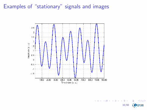
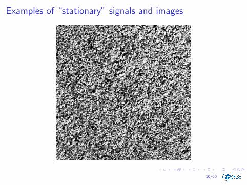
Examples of “stationary” signals and images
10/60
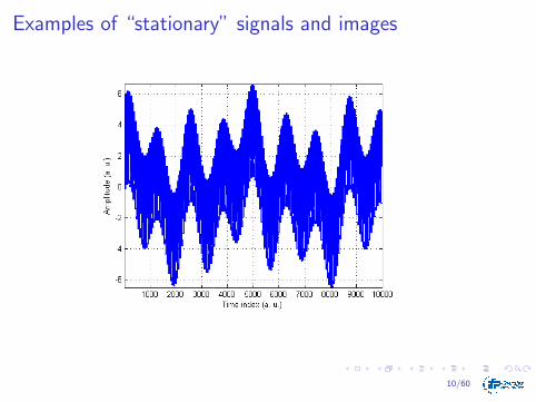
Examples of “stationary” signals and images
10/60
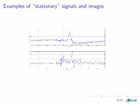
Examples of “stationary” signals and images
10/60

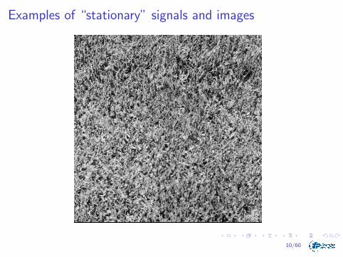
Examples of “stationary” signals and images
10/60

Examples of “stationary” signals and images
10/60

Examples of “stationary” signals and images
10/60
Examples of “stationary” signals and images
10/60

Examples of “stationary” signals and images
10/60
Examples of “stationary” signals and images
10/60

Examples of “stationary” signals and images
10/60
Examples of “stationary” signals and images
10/60

Examples of “stationary” signals and images
10/60
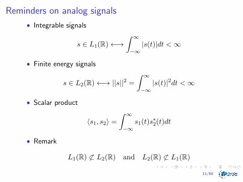
Reminders on analog signals
• Integrable signals
s ∈ L1(R)←→∫ ∞−∞|s(t)|dt <∞
• Finite energy signals
s ∈ L2(R)←→ ||s||2 =
∫ ∞−∞|s(t)|2dt <∞
• Scalar product
〈s1, s2〉 =
∫ ∞−∞
s1(t)s∗2(t)dt
• Remark
L1(R) 6⊂ L2(R) and L2(R) 6⊂ L1(R)
11/60

Reminders - Counter-example 1
• Signal in L2(R) but not in L1(R)
x =
{1 if |t| < 11|t| otherwise.
12/60

Reminders - Counter-example 1
• Signal L1(R) but not in L2(R)
x =
{1√t
if |t| < 1
0 otherwise.
13/60

History
A few names in the history:
• Joseph Fourier: 1807 (heat equation) [1768-1830]
• Gauß: 1805 (interpolation of orbits of celestial bodies)
• Runge: 1903
• Danielson-Lanczos: 1942
• Good: 1958
• Cooley-Tuckey: 1965 (FFT)
• Frigo-Johnson: 1998 (Fastest Fourier Transform in the West)
Source: Gauß and the history of the Fourier transform. Heideman,Johnson, Burrus, IEEE ASSP Magazine, 1984
14/60

History
Lettre de C. Jacobi a A. Legendre, 1830
M. Fourier avait l’opinion que le but principal desmathematiques etait l’utilite publique et l’explication desphenomenes naturels; mais un philosophe comme luiaurait du savoir que le but unique de la science, c’estl’honneur de l’esprit humain, et que sous ce titre, unequestion de nombres vaut autant qu’une question dusysteme du monde.
15/60
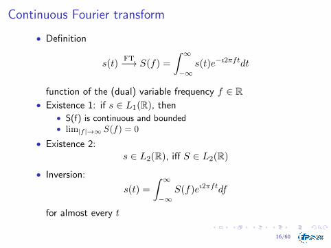
Continuous Fourier transform
• Definition
s(t)FT−→ S(f) =
∫ ∞−∞
s(t)e−ı2πftdt
function of the (dual) variable frequency f ∈ R• Existence 1: if s ∈ L1(R), then
• S(f) is continuous and bounded• lim|f |→∞ S(f) = 0
• Existence 2:s ∈ L2(R), iff S ∈ L2(R)
• Inversion:
s(t) =
∫ ∞−∞
S(f)eı2πftdf
for almost every t
16/60

Fourier transform - properties 1
• Linearity
s1(t)FT−→ S1(f), s2(t)
FT−→ S2(f)
then
∀(λ, µ) ∈ C2 λs1(t) + µs2(t)FT−→ λS1(f) + µS2(f)
• Delay/translation
∀b ∈ R, s(t− b) FT−→ e−ı2πbfS(f)
delay/translation invariance in amplitude spectrum
• Modulation:
∀ν ∈ R, eı2πνts(t)FT−→ S(f − ν)
17/60

Fourier transform - properties 2
• Scale change
∀α ∈ R∗, s(αt)FT−→ 1
|α|S(f
α)
turns dilatation onto contraction
• Time inverse: a special case
s(−t) FT−→ S(−f)
• Conjugation
s∗(t)FT−→ S∗(−f)
• Hermitian symmetry: if s is real, then:• Re(S(f)) even, Im(S(f)) odd• |S(f)| even, argS(f) odd (mod 2π)
18/60

Fourier transform - properties 3
• Convolution
(s1 ∗ s2)(t) =
∫ ∞−∞
s1(u)s2(t− u)du = (s2 ∗ s1)(t)
• Conditions• s1 ∈ L1(R), s2 ∈ L1(R)⇒ s1 ∗ s2 ∈ L1(R)• s1 ∈ L2(R), s2 ∈ L2(R)⇒ s1 ∗ s2 ∈ L2(R)
(s1 ∗ s2)(t)FT−→ S1(f)S2(f)
• Parseval-Plancherel equalities: if s1, s2 ∈ L1(R):• 〈s1, s2〉 = 〈S1, S2〉• ‖s‖2 = ‖S‖2
19/60

Fourier transform - examples
• s(t) = e−atu(t),<(a) > 0:S(f) = 1
a+2ıπf
• s(t) = e−at cos(2πf0t)u(t):
S(f) = 12
[1
a+2πı(f−f0) + 1a+2πı(f+f0)
]• s(t) = e−a|t|:
S(f) = 2|a|a2+(2πf)2
20/60

Digital signals - sampling
• For a signal s(t), regularly sampled:
s[k] = s(kT )
with T : sampling period; fs = 1/T : sampling frequency
• Sampling theorem: if S(f) = 0 for |f | ≥ B and fs ≥ 2B, thethe signal is sampled without information loss (theoretically),with Shannon-Nyquist formula:
s(t) =
∞∑k=−∞
s[k]sinc
(π(t− kT )
T
), sinc(t) =
{sin(t)t if t 6= 01 otherwise.
• cardinal theorem of interpolation theory: (Cauchy)-Whittaker,1915; Nyquist, 1928; Kotelnikov, 1933; Whittaker, 1935;Raabe, 1938; Gabor, 1946; Shannon, 1948; Someya, 1949
• Note: Balian-Low theorem for time-frequency analysis
21/60
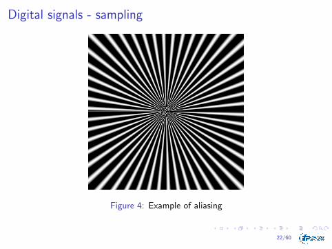
Digital signals - sampling
Figure 4: Example of aliasing
22/60

Digital signals - sampling
• Comments• sufficient but non-necessary condition• two-part theorem: (1) sampling, (2) reconstruction• caution: jitter, amplitude quantization, noise• slow convergence of the sinc, instability• signals cannot be time-limited and frequency-bounded• extensions to band-limited signals exist (iterative
Papoulis-Gerchberg); optimally 2(fu − fl). Aliases in ± freq.content do not overlap for integer k:
2fuk≤ fs ≤
2flk − 1
• alternatives: non-regularly sampled data (Lomb-Scargleperiodogram); sparse/finite-rate-of-innovation signals (no morethan n events per unit of time): compressive sensing, sparsesampling
• Beware of weak analogies between continuous/discrete
23/60

Digital signals
• Absolutely convergent sequences
(s[k])k∈Z ∈ l1(R)⇔∞∑
k=−∞|s[k]| <∞
• Square-summable sequences
(s[k])k∈Z ∈ l2(R)⇔∞∑
k=−∞|s[k]|2 <∞
• Remarkl1(R) ⊂ l2(R)
24/60

Discrete-Time Fourier transform (DTFT)
• Definition 1: z-transform
(s[k])k∈ZZT−→ S(z) =
∞∑k=−∞
s[k]z−k
• Definition 2: Discrete-Time Fourier transform
(s[k])k∈ZDTFT−→ S(f) =
∞∑k=−∞
s[k]z−k, z = eı2πf
25/60

Discrete-Time Fourier transform (DTFT)
• Normalized frequency
f = Tfphys
• Periodicityf = 1 : S(f + 1) = S(f)
• Existence(s[k])k∈Z ∈ l2(R)
• Special case: if (s[k])k∈Z ∈ l1(R), then S(f) is continuousand bounded
26/60

DTFT - properties 1
• Linearity
λs1[k] + µs2[k]DTFT−→ λS1(f) + µS2(f)
• Integer delay/translation
s[k − n]DTFT−→ e−ı2πnfS(f)
• Modulationeı2πνs[k]
DTFT−→ S(f − ν)
• Time inversions[−k]
DTFT−→ S(−f)
27/60

DTFT - properties 2
• Conjugaison
s∗[k]DTFT−→ S∗(−f)
• Parseval-Plancherel equalities
∞∑k=−∞
s1[k]s∗2[k] =
∫ 1/2
−1/2S1(f)S∗2(f)df
∞∑k=−∞
|s[k]|2 =
∫ 1/2
−1/2|S(f)|2df
28/60

DTFT - properties 3
• Convolution
(s1 ∗ s2)[k] =
∞∑l=−∞
s1[l]s2[k − l]DTFT−→ S1(f)S2(f)
• Inversion
s[k] =
∫ 1/2
−1/2S(f)eı2πfkdf
29/60

Fourier series
• If s is periodic (and continuous), s(t+ 2π) = s(t) define:
a0 =1
π
∫ −π−π
s(t)
ak =1
π
∫ −π−π
s(t) cos(kt)dt
bk =1
π
∫ −π−π
s(t) sin(kt)dt
then the infinite Fourier series is:
s(t) ' a02
+
∞∑k=1
[ak cos(kt) + bk sin(kt)]
30/60
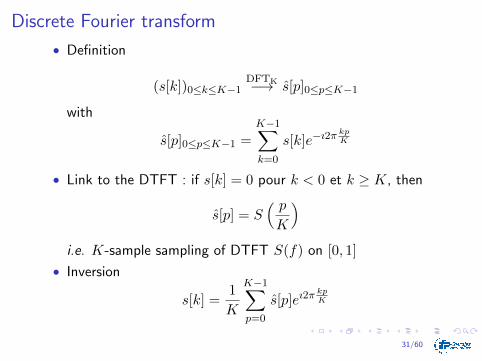
Discrete Fourier transform
• Definition
(s[k])0≤k≤K−1DFTK−→ s[p]0≤p≤K−1
with
s[p]0≤p≤K−1 =
K−1∑k=0
s[k]e−ı2πkpK
• Link to the DTFT : if s[k] = 0 pour k < 0 et k ≥ K, then
s[p] = S( pK
)i.e. K-sample sampling of DTFT S(f) on [0, 1]
• Inversion
s[k] =1
K
K−1∑p=0
s[p]eı2πkpK
31/60
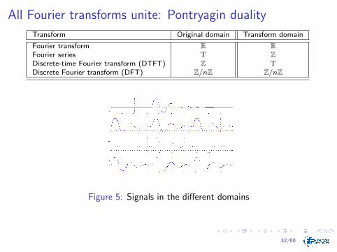
All Fourier transforms unite: Pontryagin duality
Transform Original domain Transform domain
Fourier transform R RFourier series T ZDiscrete-time Fourier transform (DTFT) Z TDiscrete Fourier transform (DFT) Z/nZ Z/nZ
Figure 5: Signals in the different domains
32/60

Fast Fourier transform - FFT
• Fast algorithms exist (since Gauss)
FFTK ⇒ complexity of O(K log2(K)) operations
• Cyclic or periodic convolution: Let (s1[k])0≤k≤K−1 and(s2[k])0≤k≤K−1
(s1 ∗©s2)[k]DFTK−→ s1[p] · s2[p]
where (s1 ∗©s2)[k] represents the K-point convolution of theperiodized sequences:
(s1 ∗©s2)[k] =
k∑l=0
s1[l]s2[k − l] +
K−1∑l=k+1
s1[l]s2[K + k − l]
33/60

Reminders - Key message
• Nature of the data and the transform• Continuous and discrete natures ARE different• Generally stuff works• Intuition may be misleading (ex.: FFT on 8-sample signals,
non proper windows)• Sometimes special care is needed: re-interpolation,
pre-processing to avoid edge effects, instabilities, outliers
34/60

Windows• Several uses
• apodization, tapering (edges, jumps)• ”stationarizing”• spectral estimation, filter design
Figure 6: Windows in the original domain
• Many (parametric) designs:• Rect., Bartlett, Hann, Hamming, Kayser, Chebychev,
Blackman-Harris,...• Gen. cosine: a0 − a1 cos( 2πn
M−1 ) + a2 cos( 4πnM−1 )− a3 cos( 6πn
M−1 )
35/60

Windows• Several uses
• apodization, tapering (edges, jumps)• ”stationarizing”• spectral estimation, filter design
Figure 6: Windows in the frequency domain
• Many (parametric) designs:• Rect., Bartlett, Hann, Hamming, Kayser, Chebychev,
Blackman-Harris,...• Gen. cosine: a0 − a1 cos( 2πn
M−1 ) + a2 cos( 4πnM−1 )− a3 cos( 6πn
M−1 )
35/60

Side dishes - Hilbert transform
• Linear operator (Cauchy kernel)
• Important tool in signal processing, mechanics, waves
Hf(t) =1
πp.v.
∫ +∞
−∞
f(s)
t− sds
F(Hf(t))(ω) = (−ısign(ω)).F(f)(ω)
• Analytic signal: f(t) = f(t) + ıHf(t)
• Examples of Hilbert pairs:• cos(t)→ sin(t) (eıt) (cisoid)• 1
1+t2 →t
1+t2
• Useful for envelope extraction, inst. freq. estimation,time-frequency processing
36/60

Side dishes - Hilbert transform and pairsReminders [Gabor-1946][Ville-1948]
H{f}(ω) = −ısign(ω)f(ω)
Figure 7: Hilbert pair 1
37/60

Side dishes - Hilbert transform and pairsReminders [Gabor-1946][Ville-1948]
H{f}(ω) = −ısign(ω)f(ω)
Figure 7: Hilbert pair 2
37/60

Side dishes - Hilbert transform and pairsReminders [Gabor-1946][Ville-1948]
H{f}(ω) = −ısign(ω)f(ω)
Figure 7: Hilbert pair 3
37/60

Side dishes - Hilbert transform and pairsReminders [Gabor-1946][Ville-1948]
H{f}(ω) = −ısign(ω)f(ω)
Figure 7: Hilbert pair 4
37/60
Reminders: set averages
• s(n): discrete time random process (stationary stochasticprocess)
• expectation:µs(n) = E{s(n)}
• variance:σ2s(n) = E{|s(n)− µs(n)|2}
• autocovariance:
cs(k, l) = E{(s(k)− µs(k))(s(l)− µs(l))∗}
38/60

Reminders: power spectral densityFor an autocorrelation ergodic process:
limN→∞
1
2N + 1
N∑n=−N
s(n+ k)s(n) = rss(k)
• if s(n) is known for every n, power spectrum estimation• caveat 1: samples are not unlimited [0, . . . , N − 1], sometimes
small• caveat 2: corruption (noise, interfering signals)
Recast the problem: from the biased estimator of the ACF
rss(k) =
N−1−k∑n=0
s(n+ k)s(n)
estimate power spectrum (periodogram)
Px(eıω) =
N−1∑k=−N+1
rss(k)eıkω
39/60

Time and frequency resolution
• Energy
E =
∫|s(t)|2dt =
∫|S(f)|2df
• Time or frequency location
t = 1/E
∫t|s(t)|2dt f = 1/E
∫f |S(f)|2df
• Energy dispersion
∆t =
√1/E
∫(t− t)2|s(t)|2dt
∆f =
√1/E
∫(f − f)2|S(f)|2df
40/60

Heisenberg-Gabor inequality
• Theorem (Weyl, 1931)If s(t), ts(t), s′(t) ∈ L2 then
‖s(t)‖2 ≤ 2‖ts(t)‖‖s′(t)‖
• Equality:Iff s(t) is a modulated Gaussian/Gabor elementary function:
s′(t)/s(t) ∝ t
s(t) = C exp[−α(t− tm)2 + ı2πνm(t− tm)]
• ProofIntegration by part + Cauchy-Schwarz
41/60

Uncertainty principle (UP)
• Time-frequency UPFor finite-energy every signal s(t), with ∆t and ∆f finite:
∆t∆f ≥ 1
4π
with equality for the modulated Gaussian only
• Principles‖s′(t)‖2 = |ı2π|2‖fS(f)‖2
• Observations• Fourier (continuous) fundamental limit: arbitrary ”location”
cannot be attained both in time and frequency• have to choose between time and frequency locations• Gaussians are ”the best”
42/60

Uncertainty principle (UP) for project management
Applies to other domains
Figure 8: Dilbert
43/60

Uncertainty principle - time
• One may write
s(t) =
∫s(u)δ(t− u)du
• δ(t) is neutral w.r.t. convolution• interpreted as a decomposition of s(t) onto a basis of shiftedδ(t− u): ∆t = 0 at
• FT of basis functions: e−ı2πft: ∆f =∞
UP: as a limit of 0×∞
44/60

Uncertainty principle - frequency
• One may write
s(t) =
∫S(f)eı2πftdf
• interpreted as a decomposition on pure waves eı2πft: ∆t =∞• FT of basis functions: δ(f − t) : ∆f = 0
UP: as a limit of ∞× 0
45/60

Uncertainty principle - illustration
46/60

Basis formalism interpretation
• Orthonormality
〈eı2πft, eı2πgt〉 = δ(f − g)
〈δ(f), δ(g)〉 = δ(f − g)
• Scalar productS(f) = 〈s(t), eı2πft〉
s(t) = 〈s(t), δ(f)〉• Matching of a signal with a vector, a basis function (pure
wave, Dirac)• Synthesis: continuous sum of orthogonal projection onto basis
functions• Relative interest of the two bases? Other bases?
(Walsh-Hadamard, DCT, eigenbase)• How to cope with mixed resolution?
47/60

Sliding window Fourier transform
• PrinciplesFourier analysis on time-space slices of the continuous s(t)with a sliding window h(t− τ)
• Short-term/short-time Fourier transform (STFT)
Ss(τ, f ;h) =
∫s(t)h∗(t− τ)e−ı2πftdt
• Wider domain of applications than FT• depend on h• FT as a peculiar instance (valid for other transforms: not a
new tool, only a more versatile ”leatherman”-like multi-tool)
48/60

Sliding window Fourier transform
Figure 9: Leatherman wave black
49/60
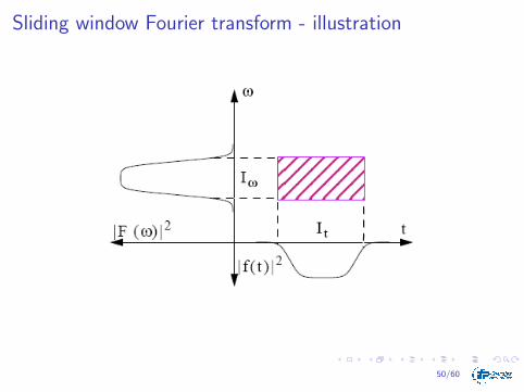
Sliding window Fourier transform - illustration
50/60

Sliding window Fourier transform - time-freq. completude
Notion of a ”complete” descrition (i.e. somehow invertible)
51/60

Sliding window Fourier transform - windows
• Related to frequency analysisDepend on the window choice h (shape, length)
• Continuous time windows• rectangular: poor frequency resolution• gaussian: best time-frequency trade-off? (Gabor, 1946)
• Discrete time windows• τ discretized (jumps vs. redundancy)• different criteria: side lobes, equiripple, apodizing; Bartlett,
Hamming, Hann, Blackmann-Harris, Blackmann-Nutall,Kaiser, Chebychev, Bessel, Generalized raised cosine, Lanczos,Flat-top,...
52/60

Sliding window Fourier transform - paving
53/60

Sliding window Fourier transform - reconstruction
• Simple analogy• synthesis: what two numbers add to result 3• a+ b = 3: infinite number of solutions, e.g.
2945.75 + (−2942.75) but irrelevant• assume they are integers?• assume they are positive? 1 + 2 = 3 or 2 + 1 = 3• aim: increase interpretability, information compaction
(0 + 3 = 3), reduce overshoot
54/60

Sliding window Fourier transform - reconstruction
• Redundant transformation!
• Inversion
s(t) =
∫ +∞
−∞
∫ +∞
−∞Ss(u, ξ;h)g(t− u)eı2πtududξ,
provided that ∫ +∞
−∞g(t)h∗(t)dt = 1.
(perfect reconstruction, no information loss)• special case: admissible normalized window h
g(t) = h(t)
but not the only solution (truncated sin)• a bit more involved for discrete time, less if only approximate
55/60

Sliding window Fourier transform - spectrogram
• Definition|Ss(τ, f ;h)|2
• The spectrogram is a (bilinear) time-frequency distribution
E =
∫∫|Ss(τ, f ;h)|2dτdf
for normalized admissible window h
• Parseval formula
〈s1, s2〉 =
∫∫Ss1(τ, f ;h)Ss2(τ, f ;h)dτdf
56/60

Sliding window Fourier transform - monoresolution
• Reason: basis functions
h(t− τ)eı2πft
all possess similar resolution
• Examples:• s(t) = δ(t− t0) −→ |Ss(τ, f ;h)|2 = |h(t0 − τ)|2• s(t) = eı2πf0t −→ |Ss(τ, f ;h)|2 = |H(f0 − f)|2
• Uses• for long range oscillatory signals, long windows are necessary• for short range transient, short windows needed• possibility to use several in parallel• incentive to use several ones simultaneously
57/60

Sliding window Fourier transform - illustration
58/60

Other time frequency distributions
• Quadratic or bilinear distributions• Wigner-Ville and avatars (smoothed, pseudo-, reweighted)• Cohen class (WV, Rihaczek, Born-Jordan, Choi-Williams)• property based: covariance, unitarity, inst. freq. & group delay,
localization (for specific signals), support preservation,positivity, stability, interferences
• Bertrand class, fractional Fourier transforms, linear canonicaltransformation (4 param.: FT, fFT, Laplace,Gauss-Weierstrass, Segal-Bargmann, Fresnel transforms)
• generally not applied in more than 1-D
59/60

Conclusions and perpectives
• Time-scale/time-frequency
• tools adapted to non-stationarity• may be adapted in scale/frequency• flexible choice of tools• flexible choice of sampling/redundancy
• deterministic processing• 1D: trends, oscillations, singularities• nD: low-dimensional singularities, edges, textures
• non-deterministic processing• noise, fractals, brownian processes
• high hybridization potential• parametric modeling, statistics, heuristic, local learning
• Very active research
60/60