Traders and Credit Constrained Farmers: Market Power

along Indonesian Rubber Value Chains

Thomas Kopp1 and Bernhard Brummer1

1Georg August University, Gottingen, Germany

Abstract

While traders of agricultural products are known to often exercise market

power, this power has rarely been quantified for developing countries. In

order to derive a measure, we estimate the traders’ revenue functions and

calculate the Marginal Value Products directly from them. We subsequently

find determinants affecting their individual market power. An exceptional

data set with detailed information on the business practices of rubber traders

in Jambi, Indonesia is employed. Results show that market power at the

traders’ level exists and is substantial. This market power is amplified in

situations of extreme remoteness, and weakens with increasing market size.

1 Introduction

It is widely recognized that traders and middlemen of agricultural raw products

are able to exercise a certain amount of market power, contradicting standard

economic theory of perfect arbitrage and zero profits (Aker, 2010; Subramanian

and Qaim, 2011; Piyapromdee et al., 2014). Osborne (2005) argues that the body

of literature on intermediaries of agricultural markets is extensive when looking at

the markets of industrialised economies. Southern markets, however, have rarely

been studied in this respect although it is to be expected that monopsonistic pricing

might be much more pronounced there: ‘traders in a typical source market engage

in imperfectly competitive behaviour in purchasing from farmers’ (Osborne, 2005,

p. 1).

Some newer studies address this gap in the literature and pay attention to the role

of traders. Most of these studies aim to find reasons behind the bad integration

of agricultural markets in economically less developed countries, while only a few

base their analysis on information stemming from traders. Fafchamps and Gabre-

Madhin (2006) use data from a trader survey to quantify transaction costs, focusing

1 Introduction

on the cost of information. Fafchamps and Hill (2008) record prices paid at several

stages of the value chain (including the farm gate) to collect evidence of market

power, leading to imperfect price transmission. The abovementioned study by Aker

(2010) analyses the effects of increased mobile telecommunication on the dispersion

of prices. Even fewer studies estimate traders’ production functions. Fafchamps

and Minten (2002) estimate production functions to quantify the effect of social

capital on the traders’ levels of productivity.

No study was found to use traders’ production functions for finding evidence of

market power. This might be due to several reasons: firstly, it is difficult to measure

the prices of the various outputs (i. e. services) offered by these individuals, such as

changing the location of a good, or of providing credit. Besides that, in many cases

the data on firms’ individual output prices is not available at the level of detail

required (Mairesse and Jaumandreu, 2005).

Our study investigates traders’ market power by comparing the marginal value

products (MVPs) of the agricultural raw input to their observed market price.

A unique set of original survey data on Indonesian rubber traders – including

detailed output prices on an individual level – enables us to estimate the traders’

revenue functions and calculate the MVPs directly from them. The comparison

to the observed market price is operationalised by calculating Lerner Indices (the

normalised difference between market and observed prices) which are shown to be

significantly different from zero. The traders exercise monopsonistic market power.

In a subsequent step, we search for determinants that influence this market power.

Our results suggest that market imperfections such as high transaction costs (typ-

ical for remote areas) increase the imbalance. Factors that reduce the traders’

ability to exercise power are the size of the market, such as the agricultural area

dedicated to cash crop production, and the number of traders operating in the area.

This paper is structured as follows: the data used in this study is introduced

in section two. Section three provides background information on the Jambinese

rubber market and the business practices of the subjects of this analysis – the

traders and middlemen. The empirical methods and data are discussed in sections

three and four, respectively. Section five presents the results, before conclusions

are drawn in section six.

2 Data

2 Data

The data that this study is based on were generated during a survey taking place

from September to December 2012 in five districts of the Jambi Province on Suma-

tra, Indonesia in a joint project between the universities of Gottingen, Jambi, and

Bogor.1 These five districts are the primary production areas of rubber in Jambi.

In these five districts, 40 villages were selected randomly, stratified on a sub-district

level (Faust et al., 2013). The total population of rubber traders in these 40 villages

could be determined by a snowball-like search in the survey phase and totals to 313

individuals. Out of these, 221 were interviewed, which is equivalent to a response

rate of 71%. All prices, values, and quantities refer to September 2012. Since the

figures mainly stem from accounting documents of the respondents, a high level of

accuracy can be assumed (if no accounting was available, we relied on recall data).

The traders were asked about details of the three most important buyers whom

they deliver to.2 It is safe to assume that this covers all their buyers because 99%

of the respondents sell to only one or two.

3 Background: rubber in Jambi

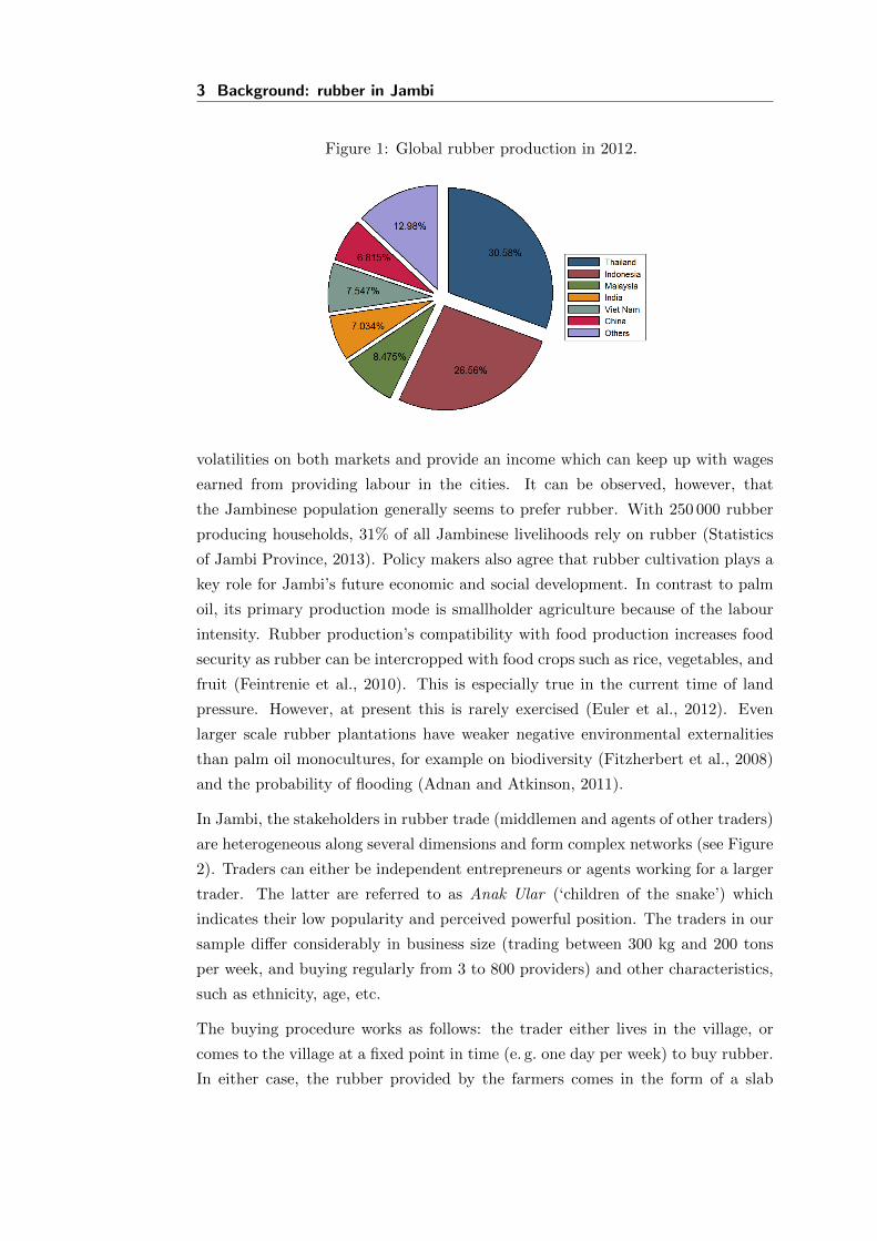
Why did we select rubber and the Jambi province? The fact that raw rubber

has a high value per volume compared to other raw products and is not perish-

able makes it an extensively traded good that can be moved along complex value

chains. Jambi is representative of a rubber producing province in Indonesia, the

second largest producer in the world (see figure 1).3 Rubber is also important

for the Jambi province in particular and is seen by policy makers as one key for

reducing unemployment and poverty (Feintrenie et al., 2010). This all makes it

an interesting case study for the application of the proposed method of estimating

revenue functions in order to find evidence for market power.

Today, rubber is the main commodity produced by smallholders in Jambi. Jambi

is a key producer of palm oil too, but a lot of this production takes place in the

form of large scale plantation agriculture while rubber is predominantly produced

by smallholders. Martini et al. (2010) argue that a mixed portfolio of rubber

and palm oil would be the best strategy for smallholders to insure against price

1Collaborative Research Centre 990: http://www.uni-goettingen.de/en/310995.html.2We thank Jenny Aker (Tufts University), Todd Benson (IFPRI, Kampala), and Ruth Vargas

Hill (IFPRI, Washington) who were so kind to provide the blank questionnaires they used for their

respective trader surveys.3Figure based on data from FaoStat (accessed on 08.10.2014).

3 Background: rubber in Jambi

Figure 1: Global rubber production in 2012.

volatilities on both markets and provide an income which can keep up with wages

earned from providing labour in the cities. It can be observed, however, that

the Jambinese population generally seems to prefer rubber. With 250 000 rubber

producing households, 31% of all Jambinese livelihoods rely on rubber (Statistics

of Jambi Province, 2013). Policy makers also agree that rubber cultivation plays a

key role for Jambi’s future economic and social development. In contrast to palm

oil, its primary production mode is smallholder agriculture because of the labour

intensity. Rubber production’s compatibility with food production increases food

security as rubber can be intercropped with food crops such as rice, vegetables, and

fruit (Feintrenie et al., 2010). This is especially true in the current time of land

pressure. However, at present this is rarely exercised (Euler et al., 2012). Even

larger scale rubber plantations have weaker negative environmental externalities

than palm oil monocultures, for example on biodiversity (Fitzherbert et al., 2008)

and the probability of flooding (Adnan and Atkinson, 2011).

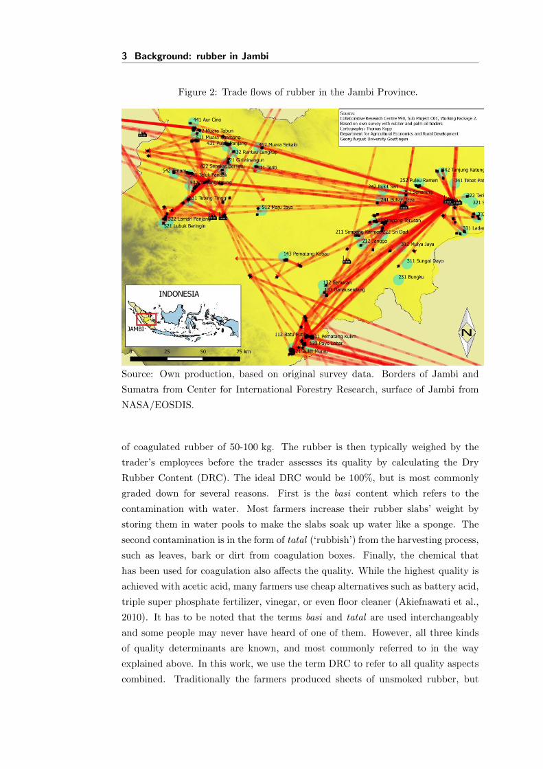
In Jambi, the stakeholders in rubber trade (middlemen and agents of other traders)

are heterogeneous along several dimensions and form complex networks (see Figure

2). Traders can either be independent entrepreneurs or agents working for a larger

trader. The latter are referred to as Anak Ular (‘children of the snake’) which

indicates their low popularity and perceived powerful position. The traders in our

sample differ considerably in business size (trading between 300 kg and 200 tons

per week, and buying regularly from 3 to 800 providers) and other characteristics,

such as ethnicity, age, etc.

The buying procedure works as follows: the trader either lives in the village, or

comes to the village at a fixed point in time (e. g. one day per week) to buy rubber.

In either case, the rubber provided by the farmers comes in the form of a slab

3 Background: rubber in Jambi

Figure 2: Trade flows of rubber in the Jambi Province.

Source: Own production, based on original survey data. Borders of Jambi and

Sumatra from Center for International Forestry Research, surface of Jambi from

NASA/EOSDIS.

of coagulated rubber of 50-100 kg. The rubber is then typically weighed by the

trader’s employees before the trader assesses its quality by calculating the Dry

Rubber Content (DRC). The ideal DRC would be 100%, but is most commonly

graded down for several reasons. First is the basi content which refers to the

contamination with water. Most farmers increase their rubber slabs’ weight by

storing them in water pools to make the slabs soak up water like a sponge. The

second contamination is in the form of tatal (‘rubbish’) from the harvesting process,

such as leaves, bark or dirt from coagulation boxes. Finally, the chemical that

has been used for coagulation also affects the quality. While the highest quality is

achieved with acetic acid, many farmers use cheap alternatives such as battery acid,

triple super phosphate fertilizer, vinegar, or even floor cleaner (Akiefnawati et al.,

2010). It has to be noted that the terms basi and tatal are used interchangeably

and some people may never have heard of one of them. However, all three kinds

of quality determinants are known, and most commonly referred to in the way

explained above. In this work, we use the term DRC to refer to all quality aspects

combined. Traditionally the farmers produced sheets of unsmoked rubber, but

3 Background: rubber in Jambi

had to switch to the production of thick slabs due to policy changes in the early

1970s, after which only the export of Technically Specified Rubber was allowed

and lower grades were prohibited (Pitt, 1980). The disadvantage from the farmers’

perspective is that the quality of unsmoked rubber sheets is less variable than the

quality of slabs, which are therefore more prone to manipulation.

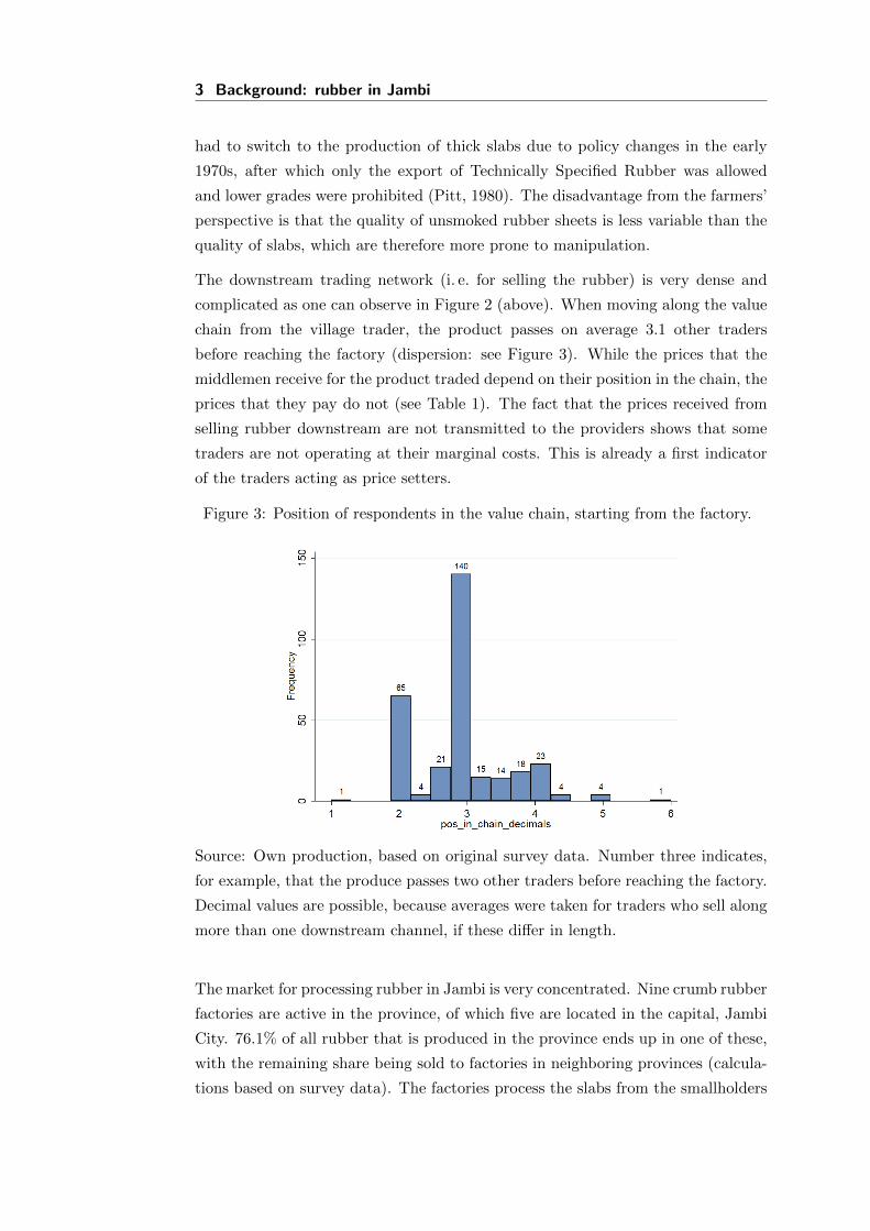
The downstream trading network (i. e. for selling the rubber) is very dense and

complicated as one can observe in Figure 2 (above). When moving along the value

chain from the village trader, the product passes on average 3.1 other traders

before reaching the factory (dispersion: see Figure 3). While the prices that the

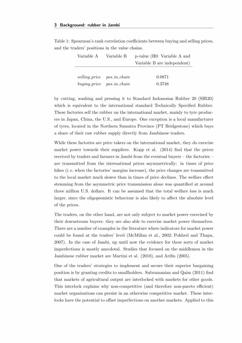
middlemen receive for the product traded depend on their position in the chain, the

prices that they pay do not (see Table 1). The fact that the prices received from

selling rubber downstream are not transmitted to the providers shows that some

traders are not operating at their marginal costs. This is already a first indicator

of the traders acting as price setters.

Figure 3: Position of respondents in the value chain, starting from the factory.

Source: Own production, based on original survey data. Number three indicates,

for example, that the produce passes two other traders before reaching the factory.

Decimal values are possible, because averages were taken for traders who sell along

more than one downstream channel, if these differ in length.

The market for processing rubber in Jambi is very concentrated. Nine crumb rubber

factories are active in the province, of which five are located in the capital, Jambi

City. 76.1% of all rubber that is produced in the province ends up in one of these,

with the remaining share being sold to factories in neighboring provinces (calcula-

tions based on survey data). The factories process the slabs from the smallholders

3 Background: rubber in Jambi

Table 1: Spearman’s rank correlation coefficients between buying and selling prices,

and the traders’ positions in the value chains.

Variable A Variable B p-value (H0: Variable A and

Variable B are independent)

selling price pos in chain 0.0871

buying price pos in chain 0.3748

by cutting, washing and pressing it to Standard Indonesian Rubber 20 (SIR20)

which is equivalent to the international standard Technically Specified Rubber.

These factories sell the rubber on the international market, mainly to tyre produc-

ers in Japan, China, the U.S., and Europe. One exception is a local manufacturer

of tyres, located in the Northern Sumatra Province (PT Bridgestone) which buys

a share of their raw rubber supply directly from Jambinese traders.

While these factories are price takers on the international market, they do exercise

market power towards their suppliers. Kopp et al. (2014) find that the prices

received by traders and farmers in Jambi from the eventual buyers – the factories –

are transmitted from the international prices asymmetrically: in times of price

hikes (i. e. when the factories’ margins increase), the price changes are transmitted

to the local market much slower than in times of price declines. The welfare effect

stemming from the asymmetric price transmission alone was quantified at around

three million U.S. dollars. It can be assumed that the total welfare loss is much

larger, since the oligopsonistic behaviour is also likely to affect the absolute level

of the prices.

The traders, on the other hand, are not only subject to market power exercised by

their downstream buyers: they are also able to exercise market power themselves.

There are a number of examples in the literature where indicators for market power

could be found at the traders’ level (McMillan et al., 2002; Pokhrel and Thapa,

2007). In the case of Jambi, up until now the evidence for these sorts of market

imperfections is mostly anecdotal. Studies that focused on the middlemen in the

Jambinese rubber market are Martini et al. (2010), and Arifin (2005).

One of the traders’ strategies to implement and secure their superior bargaining

position is by granting credits to smallholders. Subramanian and Qaim (2011) find

that markets of agricultural output are interlocked with markets for other goods.

This interlock explains why non-competitive (and therefore non-pareto efficient)

market organizations can persist in an otherwise competitive market. These inter-

locks have the potential to offset imperfections on another markets. Applied to this

3 Background: rubber in Jambi

case, the initial imperfection is the constrained access of smallholders to credit. The

most prominent reasons for smallholders’ limited access to formal credit in many

developing countries are limited possibilities of contract enforcement and a lack of

collateral due to non-formal property rights (Barnett et al., 2008). Rubber traders

are traditionally providers of informal credit. Observations of our survey showed

that no collateral is needed because the credit agreement is based on trust, stem-

ming from ongoing personal interaction and close ties within the village community.

This confirmed the observations made by Akiefnawati et al. (2010). However, this

credit also increases the traders’ bargaining power tremendously, since it is ex-

pected that an indebted farmer sells his or her produce exclusively to the provider

of his or her credit. This strategy has also been reported in the cases of Benin and

Malawi: the credit’s ‘[. . . ] main purpose is not to exploit farmers’ need for cash

in order to finance agricultural production, but rather a means for traders to se-

cure future deliveries’ (Fafchamps and Gabre-Madhin, 2006, p. 36). This behaviour

could also be documented for the case of Jambi: 94.1% of the rubber traders who

provide credit answered ‘yes’ to the question ‘Does a farmer have to sell his/her

rubber/palm oil to you if he/she wants to take a credit from you?’. 72.9% replied

with ‘no’ when they were asked: ‘If a farmer/other trader owes you money, can

she sell her produce to another trader?’ (All figures for this and the following

paragraph are based on original survey data; for more information on the data see

below).

The credit not only attaches the farmers to the traders, but these traders also

manipulate the DRC level of the delivered rubber if the farmer is indebted. This

would be an implicit interest since, for cultural reasons, the traders do not officially

charge any interest on the credit. In interviews, 11.8% of the responding traders

stated that they manipulate the basi estimation for suppliers who are indebted.

This seems to be a small share, but given that this practice is understood as

immoral, it can be expected that the figure given here is underestimating the

true share because respondents might not ‘admit’ in interviews that they follow

this practice. However, it is reasonable to understand this hidden interest as the

traders’ own capital costs which they pass on to the farmers.

It is the target of this analysis to empirically verify whether Jambinese rubber

traders do indeed exercise market power towards their suppliers and – if so – what

determines the extent of it. The key question is whether factor prices of the rubber

input equal their marginal value products.

4 Methodology

4 Methodology

The intuition of our empirical approach to test for market power at the traders’

level is to estimate the revenue functions of the traders. We use these estimated

functions to directly calculate the marginal value product (MVP) of raw rubber

which would– in the situation of perfect competition – be equal to the observed

market prices that the traders pay for this input. If the latter ones were smaller,

this would be an indication of market imperfection. In a second stage, we find

determinants for deviations from the MVP by calculating Lerner Indices for each

trader, and regressing them on characteristics of the transactions (characteristics

of the geographic location, of the traders, and of the trader-provider relationships).

4.1 Model development

Berndt (1996) argues that in situations of exogenous input quantities and endoge-

nous input prices, the production (or revenue) functions need to be employed.4

The advantage over estimating a cost function is that input prices do not enter

the model which we wish to avoid, since these are the observed prices that are to

be compared to the MVPs deducted from the estimated revenue functions. ‘Pro-

duction’ is, in this case, understood as improving the value of the raw rubber that

the traders buy, for example by changing its location, i. e. providing the service of

transportation. Since the selling prices of rubber which the traders are confronted

with vary substantially between the traders – depending on whom they sell to –

the standard approach of generating the output quantity by dividing the revenue

by an industry-average of the prices would not account for these price differences

and therefore lead to a serious bias (Mairesse and Jaumandreu, 2005). Instead we

weight the output by the selling prices, resulting in the estimation of a revenue

function. Mairesse and Jaumandreu (2005) find that it does not systematically

change the estimated results if the LHS of a production function is deflated by the

output prices or not (apart from the desired effect from the weighting).

A potential problem in the estimation of traders’ production functions is one of

endogeneity: traders who are generally more efficient might handle larger volumes,

which would cause a correlation between the error term and this input quantity.

However, in Jambi it is not the trader’s choice how much rubber he or she trades,

4The reason why we do not estimate a value added function is that knowing which factors affect

the value-added would not facilitate any conclusions on market power. It would be interesting

to assess how the value added is distributed amongst all stakeholders of the value chain, but this

is not feasible within the scope of this study since it would require detailed data on the cost

structures of all stakeholders.

4.2 Application

since they usually buy everything they can get, due to the good margins. According

to Zellner et al. (1966), the problem does not apply if the choice of how much input

is used is not made by the trader. The same is true for the credit: the amount of

the credit that the traders provide is determined by their providers’ needs rather

than their own choice. The credit is, as in other settings, too (e. g. Benin and

Malawi, see Fafchamps and Gabre-Madhin, 2006), used as an instrument to attach

providers to them. Thus the output/revenue per input is not correlated to the

‘size’ of the trader.

4.2 Application

We base the specification of our model on the following transcendental revenue

function in logarithmic form (Boisvert, 1982):5

lnY = lnα0 +N∑i=1

(αi lnxi) +1

2

N∑i=1

N∑j=1

(αij lnxi lnxj) + ε (1)

Y on the LHS represents the value of the output while the xi on the RHS refer

to the quantities of the inputs. N denotes the total number of inputs and ε the

error term. For the reasons laid out above, the output enters in the form of gross

revenue. The raw rubber that the traders buy is included as an intermediary input.

Other variables that are included in the RHS are the bilateral distance between the

trader and his or her buyer as a proxy for trade costs, the weekly hours that the

traders work themselves, and their total transport capacity as a proxy for capital.

Concerning the costs of hired labour, it cannot be deduced from theory if they are

to be modelled in terms of working hours or total costs: the price of labour might

account for unobserved quality differences which would argue for using the total

costs. However, price differences might also be due to regional differences which

would be a reason for using the amount of working hours. The latter two variables

cannot enter the regression together due to double counting. We therefore estimate

three models: one without hired labour (1), one with the total labour costs (2),

and one with total hours worked (3). A Likelihood Ratio Test is then employed to

compare (2) and (3) with (1). If the reduced model is shown to represent the data

best, its results are used further on. If the models that include the hired labour

are better, the Vuong’s Closeness Test for non-nested models (Vuong, 1989) will

be employed to determine whether to use (2) or (3).

5We also estimated a Cobb Douglas function. An LR test showed that it does not represent

the data as good as the translog specification. Results are available on demand.

4.3 Requirements and properties of the revenue function

The traders produce – from their suppliers’ point of view – two services: changing

the location of the product and providing credit. However, since from the traders’

perspective their sole motivation of providing credit is to expand their market base

and to attach providers to them, this is to be understood as a (quasi-fixed) input.

Thus, the credit enters the regression on the RHS, together with the other inputs.

The DRC does not enter the revenue function, since the input amount is equal to the

output amount. This means that on the LHS the quantity is already deflated by the

output quality which is equal to the (weighted) average input quality. Accordingly,

there is no need to control for this in the revenue function.

Before taking the logarithms of all variables, they are mean-scaled in order to be

able to interpret the results as elasticities. One common challenge in the estimation

of revenue functions is the occurrence of zeros in the input variables which results in

missing values when the log is taken. This is the case – for example – if a very small

trader does not make use of hired labour. These missing zeros are handled following

Battese (1997): the observations with ln 0 are replaced by 0. An additional dummy

variable, which represents the zero-inputs, is set to one, and to zero otherwise.

The variable indicating the credit that the respective trader provides is zero in-

flated and left censored (about 50% of the respondents did not give any credit in

September 2012). So instead of normalising and taking the logs of this variable,

the inverse sine hyperbolic transformation was employed, as suggested by Burbidge

et al. (1988). Since the size of the credit given by traders is not exclusively deter-

mined by their choice, but also based on their providers’ needs, it is also plausible

to represent the credit as a dummy variable (one if credit was given). This speci-

fication was tested against the alternative of treating the credit given just like the

other inputs via an LR test which gave a prob> chi2 of 0.0771. It was therefore

decided to employ the unrestricted model.6

4.3 Requirements and properties of the revenue function

We test whether the estimated revenue function satisfies the required properties at

each data point. These are the homogeneity condition (Boisvert, 1982), as well as

the curvature properties for satisfying the conditions of positive and diminishing

marginal products for every single observation (Morey, 1986). The condition of

positive marginal products is checked by taking the partial derivatives with respect

to each of the inputs. If they are > 0 at every data point, the first condition is

fulfilled. The decreasing marginal products are clarified by taking the second-order

6The results of the alternative model can be made available upon request.

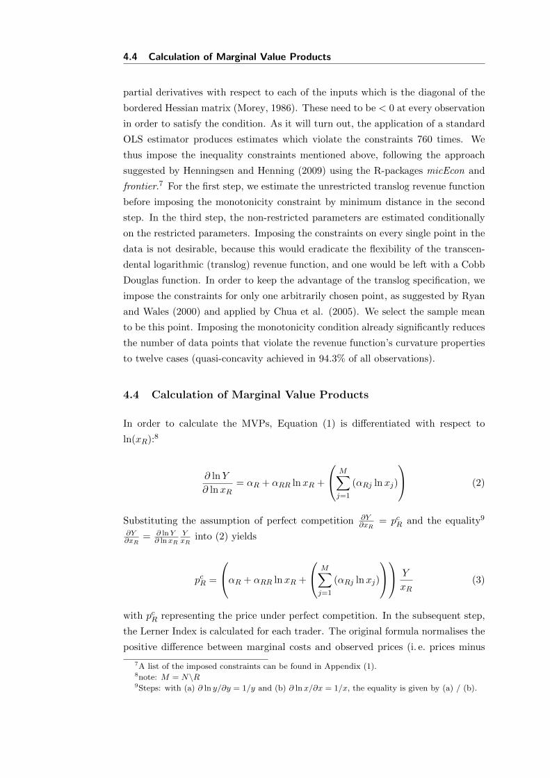
4.4 Calculation of Marginal Value Products

partial derivatives with respect to each of the inputs which is the diagonal of the

bordered Hessian matrix (Morey, 1986). These need to be < 0 at every observation

in order to satisfy the condition. As it will turn out, the application of a standard

OLS estimator produces estimates which violate the constraints 760 times. We

thus impose the inequality constraints mentioned above, following the approach

suggested by Henningsen and Henning (2009) using the R-packages micEcon and

frontier.7 For the first step, we estimate the unrestricted translog revenue function

before imposing the monotonicity constraint by minimum distance in the second

step. In the third step, the non-restricted parameters are estimated conditionally

on the restricted parameters. Imposing the constraints on every single point in the

data is not desirable, because this would eradicate the flexibility of the transcen-

dental logarithmic (translog) revenue function, and one would be left with a Cobb

Douglas function. In order to keep the advantage of the translog specification, we

impose the constraints for only one arbitrarily chosen point, as suggested by Ryan

and Wales (2000) and applied by Chua et al. (2005). We select the sample mean

to be this point. Imposing the monotonicity condition already significantly reduces

the number of data points that violate the revenue function’s curvature properties

to twelve cases (quasi-concavity achieved in 94.3% of all observations).

4.4 Calculation of Marginal Value Products

In order to calculate the MVPs, Equation (1) is differentiated with respect to

ln(xR):8

∂ lnY

∂ lnxR= αR + αRR lnxR +

M∑j=1

(αRj lnxj)

(2)

Substituting the assumption of perfect competition ∂Y∂xR

= pcR and the equality9

∂Y∂xR

= ∂ lnY∂ lnxR

YxR

into (2) yields

pcR =

αR + αRR lnxR +

M∑j=1

(αRj lnxj)

Y

xR(3)

with pcR representing the price under perfect competition. In the subsequent step,

the Lerner Index is calculated for each trader. The original formula normalises the

positive difference between marginal costs and observed prices (i. e. prices minus

7A list of the imposed constraints can be found in Appendix (1).8note: M = N\R9Steps: with (a) ∂ ln y/∂y = 1/y and (b) ∂ lnx/∂x = 1/x, the equality is given by (a) / (b).

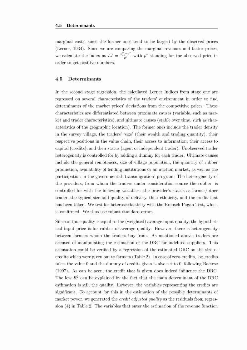
4.5 Determinants

marginal costs, since the former ones tend to be larger) by the observed prices

(Lerner, 1934). Since we are comparing the marginal revenues and factor prices,

we calculate the index as LI =pcR−p∗

p∗ with p∗ standing for the observed price in

order to get positive numbers.

4.5 Determinants

In the second stage regression, the calculated Lerner Indices from stage one are

regressed on several characteristics of the traders’ environment in order to find

determinants of the market prices’ deviations from the competitive prices. These

characteristics are differentiated between proximate causes (variable, such as mar-

ket and trader characteristics), and ultimate causes (stable over time, such as char-

acteristics of the geographic location). The former ones include the trader density

in the survey village, the traders’ ‘size’ (their wealth and trading quantity), their

respective positions in the value chain, their access to information, their access to

capital (credits), and their status (agent or independent trader). Unobserved trader

heterogeneity is controlled for by adding a dummy for each trader. Ultimate causes

include the general remoteness, size of village population, the quantity of rubber

production, availability of lending institutions or an auction market, as well as the

participation in the governmental ‘transmigration’ program. The heterogeneity of

the providers, from whom the traders under consideration source the rubber, is

controlled for with the following variables: the provider’s status as farmer/other

trader, the typical size and quality of delivery, their ethnicity, and the credit that

has been taken. We test for heteroscedasticity with the Breusch-Pagan Test, which

is confirmed. We thus use robust standard errors.

Since output quality is equal to the (weighted) average input quality, the hypothet-

ical input price is for rubber of average quality. However, there is heterogeneity

between farmers whom the traders buy from. As mentioned above, traders are

accused of manipulating the estimation of the DRC for indebted suppliers. This

accusation could be verified by a regression of the estimated DRC on the size of

credits which were given out to farmers (Table 2). In case of zero-credits, log credits

takes the value 0 and the dummy of credits given is also set to 0, following Battese

(1997). As can be seen, the credit that is given does indeed influence the DRC.

The low R2 can be explained by the fact that the main determinant of the DRC

estimation is still the quality. However, the variables representing the credits are

significant. To account for this in the estimation of the possible determinants of

market power, we generated the credit adjusted quality as the residuals from regres-

sion (4) in Table 2. The variables that enter the estimation of the revenue function

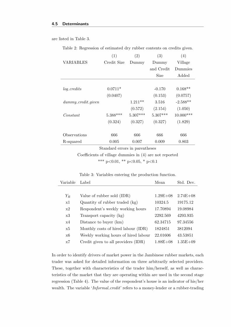
4.5 Determinants

are listed in Table 3.

Table 2: Regression of estimated dry rubber contents on credits given.

(1) (2) (3) (4)

VARIABLES Credit Size Dummy Dummy Village

and Credit Dummies

Size Added

log credits 0.0711* -0.170 0.168**

(0.0407) (0.153) (0.0757)

dummy credit given 1.211** 3.516 -2.588**

(0.572) (2.154) (1.050)

Constant 5.388*** 5.307*** 5.307*** 10.000***

(0.324) (0.327) (0.327) (1.829)

Observations 666 666 666 666

R-squared 0.005 0.007 0.009 0.803

Standard errors in parentheses

Coefficients of village dummies in (4) are not reported

*** p<0.01, ** p<0.05, * p<0.1

Table 3: Variables entering the production function.

Variable Label Mean Std. Dev.

YR Value of rubber sold (IDR) 1.29E+08 2.74E+08

x1 Quantity of rubber traded (kg) 10324.5 19175.12

x2 Respondent’s weekly working hours 17.70894 19.08984

x3 Transport capacity (kg) 2292.569 4293.935

x4 Distance to buyer (km) 62.34715 97.34556

x5 Monthly costs of hired labour (IDR) 1824851 3812094

x6 Weekly working hours of hired labour 22.01606 43.53851

x7 Credit given to all providers (IDR) 1.88E+08 1.35E+09

In order to identify drivers of market power in the Jambinese rubber markets, each

trader was asked for detailed information on three arbitrarily selected providers.

These, together with characteristics of the trader him/herself, as well as charac-

teristics of the market that they are operating within are used in the second stage

regression (Table 4). The value of the respondent’s house is an indicator of his/her

wealth. The variable ‘Informal credit ’ refers to a money-lender or a rubber-trading

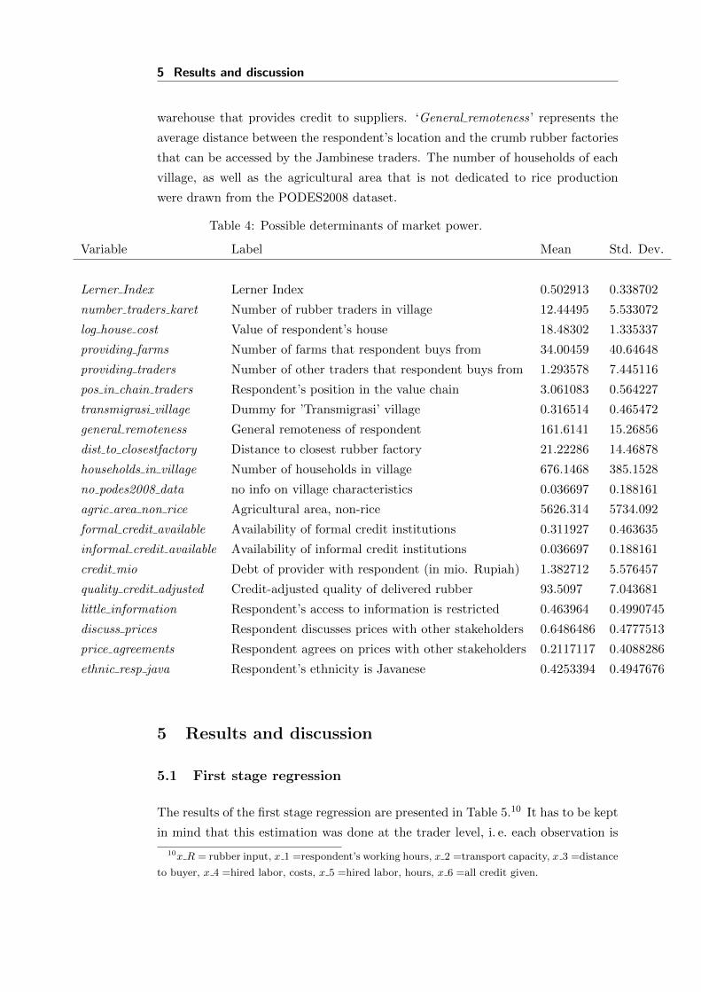
5 Results and discussion

warehouse that provides credit to suppliers. ‘General remoteness’ represents the

average distance between the respondent’s location and the crumb rubber factories

that can be accessed by the Jambinese traders. The number of households of each

village, as well as the agricultural area that is not dedicated to rice production

were drawn from the PODES2008 dataset.

Table 4: Possible determinants of market power.

Variable Label Mean Std. Dev.

Lerner Index Lerner Index 0.502913 0.338702

number traders karet Number of rubber traders in village 12.44495 5.533072

log house cost Value of respondent’s house 18.48302 1.335337

providing farms Number of farms that respondent buys from 34.00459 40.64648

providing traders Number of other traders that respondent buys from 1.293578 7.445116

pos in chain traders Respondent’s position in the value chain 3.061083 0.564227

transmigrasi village Dummy for ’Transmigrasi’ village 0.316514 0.465472

general remoteness General remoteness of respondent 161.6141 15.26856

dist to closestfactory Distance to closest rubber factory 21.22286 14.46878

households in village Number of households in village 676.1468 385.1528

no podes2008 data no info on village characteristics 0.036697 0.188161

agric area non rice Agricultural area, non-rice 5626.314 5734.092

formal credit available Availability of formal credit institutions 0.311927 0.463635

informal credit available Availability of informal credit institutions 0.036697 0.188161

credit mio Debt of provider with respondent (in mio. Rupiah) 1.382712 5.576457

quality credit adjusted Credit-adjusted quality of delivered rubber 93.5097 7.043681

little information Respondent’s access to information is restricted 0.463964 0.4990745

discuss prices Respondent discusses prices with other stakeholders 0.6486486 0.4777513

price agreements Respondent agrees on prices with other stakeholders 0.2117117 0.4088286

ethnic resp java Respondent’s ethnicity is Javanese 0.4253394 0.4947676

5 Results and discussion

5.1 First stage regression

The results of the first stage regression are presented in Table 5.10 It has to be kept

in mind that this estimation was done at the trader level, i. e. each observation is

10x R = rubber input, x 1 =respondent’s working hours, x 2 =transport capacity, x 3 =distance

to buyer, x 4 =hired labor, costs, x 5 =hired labor, hours, x 6 =all credit given.

5.2 Model choice

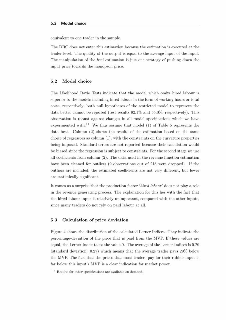
equivalent to one trader in the sample.

The DRC does not enter this estimation because the estimation is executed at the

trader level. The quality of the output is equal to the average input of the input.

The manipulation of the basi estimation is just one strategy of pushing down the

input price towards the monopson price.

5.2 Model choice

The Likelihood Ratio Tests indicate that the model which omits hired labour is

superior to the models including hired labour in the form of working hours or total

costs, respectively; both null hypotheses of the restricted model to represent the

data better cannot be rejected (test results 92.1% and 55.0%, respectively). This

observation is robust against changes in all model specifications which we have

experimented with.11 We thus assume that model (1) of Table 5 represents the

data best. Column (2) shows the results of the estimation based on the same

choice of regressors as column (1), with the constraints on the curvature properties

being imposed. Standard errors are not reported because their calculation would

be biased since the regression is subject to constraints. For the second stage we use

all coefficients from column (2). The data used in the revenue function estimation

have been cleaned for outliers (9 observations out of 218 were dropped). If the

outliers are included, the estimated coefficients are not very different, but fewer

are statistically significant.

It comes as a surprise that the production factor ‘hired labour ’ does not play a role

in the revenue generating process. The explanation for this lies with the fact that

the hired labour input is relatively unimportant, compared with the other inputs,

since many traders do not rely on paid labour at all.

5.3 Calculation of price deviation

Figure 4 shows the distribution of the calculated Lerner Indices. They indicate the

percentage-deviation of the price that is paid from the MVP. If these values are

equal, the Lerner Index takes the value 0. The average of the Lerner Indices is 0.29

(standard deviation: 0.27) which means that the average trader pays 29% below

the MVP. The fact that the prices that most traders pay for their rubber input is

far below this input’s MVP is a clear indication for market power.

11Results for other specifications are available on demand.

5.4 Second stage regression

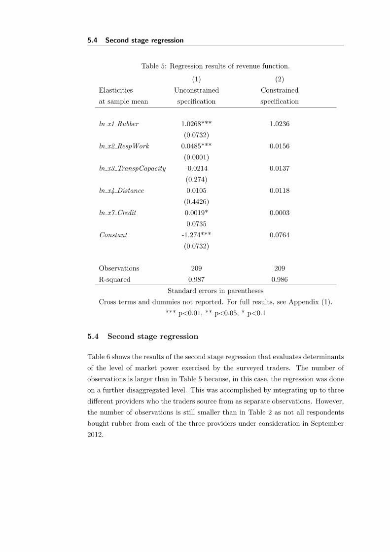
Table 5: Regression results of revenue function.

(1) (2)

Elasticities Unconstrained Constrained

at sample mean specification specification

ln x1 Rubber 1.0268*** 1.0236

(0.0732)

ln x2 RespWork 0.0485*** 0.0156

(0.0001)

ln x3 TranspCapacity -0.0214 0.0137

(0.274)

ln x4 Distance 0.0105 0.0118

(0.4426)

ln x7 Credit 0.0019* 0.0003

0.0735

Constant -1.274*** 0.0764

(0.0732)

Observations 209 209

R-squared 0.987 0.986

Standard errors in parentheses

Cross terms and dummies not reported. For full results, see Appendix (1).

*** p<0.01, ** p<0.05, * p<0.1

5.4 Second stage regression

Table 6 shows the results of the second stage regression that evaluates determinants

of the level of market power exercised by the surveyed traders. The number of

observations is larger than in Table 5 because, in this case, the regression was done

on a further disaggregated level. This was accomplished by integrating up to three

different providers who the traders source from as separate observations. However,

the number of observations is still smaller than in Table 2 as not all respondents

bought rubber from each of the three providers under consideration in September

2012.

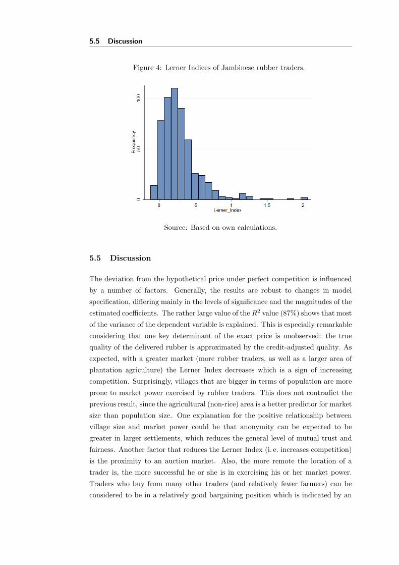
5.5 Discussion

Figure 4: Lerner Indices of Jambinese rubber traders.

Source: Based on own calculations.

5.5 Discussion

The deviation from the hypothetical price under perfect competition is influenced

by a number of factors. Generally, the results are robust to changes in model

specification, differing mainly in the levels of significance and the magnitudes of the

estimated coefficients. The rather large value of theR2 value (87%) shows that most

of the variance of the dependent variable is explained. This is especially remarkable

considering that one key determinant of the exact price is unobserved: the true

quality of the delivered rubber is approximated by the credit-adjusted quality. As

expected, with a greater market (more rubber traders, as well as a larger area of

plantation agriculture) the Lerner Index decreases which is a sign of increasing

competition. Surprisingly, villages that are bigger in terms of population are more

prone to market power exercised by rubber traders. This does not contradict the

previous result, since the agricultural (non-rice) area is a better predictor for market

size than population size. One explanation for the positive relationship between

village size and market power could be that anonymity can be expected to be

greater in larger settlements, which reduces the general level of mutual trust and

fairness. Another factor that reduces the Lerner Index (i. e. increases competition)

is the proximity to an auction market. Also, the more remote the location of a

trader is, the more successful he or she is in exercising his or her market power.

Traders who buy from many other traders (and relatively fewer farmers) can be

considered to be in a relatively good bargaining position which is indicated by an

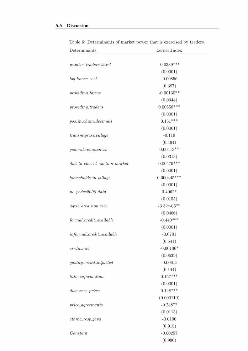
5.5 Discussion

Table 6: Determinants of market power that is exercised by traders.

Determinants Lerner Index

number traders karet -0.0339***

(0.0001)

log house cost -0.00856

(0.387)

providing farms -0.00130**

(0.0344)

providing traders 0.00558***

(0.0001)

pos in chain decimals 0.131***

(0.0001)

transmigrasi village -0.119

(0.494)

general remoteness 0.00413**

(0.0313)

dist to closest auction market 0.00479***

(0.0001)

households in village 0.000445***

(0.0001)

no podes2008 data 0.406**

(0.0155)

agric area non rice -3.32e-06**

(0.0466)

formal credit available -0.440***

(0.0001)

informal credit available -0.0701

(0.541)

credit mio -0.00106*

(0.0639)

quality credit adjusted -0.00615

(0.144)

little information 0.157***

(0.0001)

discusses prices 0.148***

(0.000110)

price agreements -0.248**

(0.0115)

ethnic resp java -0.0100

(0.915)

Constant -0.00257

(0.996)

Observations 466

R-squared 0.869

Standard errors in parentheses

Trader dummies not reported. Full results are available on demand.

*** p<0.01, ** p<0.05, * p<0.1

6 Conclusions

increasing Lerner Index. According to the data, the availability of at least one

formal credit institution reduces the market power of traders which supports the

arguments laid out in the theoretical part. However, it seems that farmers who

do get more credit from the traders are also the ones who receive better prices

compared to the ones without credits. The reason behind this is that farmers

taking relatively little credit receive a higher interest rate due to the fixed costs

of providing credit. In the context of this study, these fixed costs consist of the

time the trader invests to generate and continue personal ties with the debtor,

as well as the time spent observing him or her. While traders’ general access to

information is negatively related to their ability to exercise market power, the ones

who discuss the prices which they pay with other traders generate higher margins.

This is another indicator pointing towards collusion.

6 Conclusions

The results of this study indicate that agricultural traders in Indonesia, more specif-

ically the Jambinese rubber traders, possess monopsonistic market power. This

could be shown via an innovative approach that was enabled by an exceptional set

of data: we had access to detailed sales data on a single-transaction level. Such

data are at a much more disaggregated level than in any other examples in the lit-

erature. These data enabled the estimation of a revenue function, which was used

to directly calculate hypothetical rubber prices under the assumption of perfect

competition. The hypothetical prices were compared to the observed prices that

middlemen for rubber pay to their providers via calculating Lerner Indices. These

proved to be significantly different from zero – a clear indication of market power.

In a second stage, the Lerner Indices were regressed on different characteristics

of the market, of the traders and of the relationships between traders and their

providers. If local markets are smaller (less agricultural output, fewer traders),

the traders have more opportunities to exercise market power, as well as having

a more remote location. Improving infrastructure could reduce the influence of

‘remoteness’ on the functioning of the Jambinese rubber markets, as does the

establishment of auction markets in a larger number. Since the availability of

formal credit institutions is also negatively related to the exercise of market power,

the support of farmers through micro credit might also help.

If our explanation of the influence of village size on market power is correct (and

the verification of this certainly calls for further research), policy makers should

focus on measures improving trust and comradeship between villagers.

References

References

Adnan, N. A. and Atkinson, P. M. (2011). Exploring the impact of climate and

land use changes on streamflow trends in a monsoon catchment. International

Journal of Climatology, 31(6):815–831.

Aker, J. C. (2010). Information from markets near and far: Mobile phones and

agricultural markets in Niger. American Economic Journal: Applied Economics,

2:46–59.

Akiefnawati, R., Ayat, A., Alira, D., Suyitno, and Joshi, L. (2010). Enhancing

rubber production in communities around a village forest in Bungo District,

Jambi Province. In Leimona, B. and Joshi, L., editors, Eco-certified natural

rubber from sustainable rubber agroforestry in Sumatra, Indonesia., pages 25–31.

World Agroforestry Centre (ICRAF).

Arifin, B. (2005). Supply-Chain of Natural Rubber in Indonesia. Jurnal Manajemen

Agribisnis, 2(1):1–16.

Barnett, B. J., Barrett, C. B., and Skees, J. R. (2008). Poverty Traps and Index-

Based Risk Transfer Products. World Development, 36:1766–1785.

Battese, G. E. (1997). A Note on the Estimation of Cobb-Douglas Production

Functions when some Explanatory Variables Have Zero Values. Journal of Agri-

cultural Economics, 48:250–252.

Berndt, E. R. (1996). The Practice of Econometrics: Classic and Contemporary.

Addison Wesley, Boston, har/dskt edition.

Boisvert, R. N. (1982). The Translog Production Function - Properties, several In-

terpretations and Estimation Problems. Department of Agricultural Economics,

Cornell Univ: Working Paper.

Burbidge, J. B., Magee, L., and Robb, A. L. (1988). Alternative Transformations

to Handle Extreme Values of the Dependent Variable. Journal of the American

Statistical Association, 83:123–127.

Chua, C. L., Kew, H., and Yong, J. (2005). Airline Code-Share Alliances and Costs:

Imposing Concavity on Translog Cost Function Estimation. Review of Industrial

Organization, 26:461–487.

Euler, M., Krishna, V., Fathoni, Z., Hermanto, S., Schwarze, S., and Qaim, M.

(2012). Ecological and Socioeconomic Functions of Tropical Lowland Rain-

forest Transformation Systems (Sumatra, Indonesia), Household Survey 2012.

References

Gottingen, Germany; Jambi, Indonesia; Bogor, Indonesia; Georg-August Uni-

versity of Goettingen, Bogor Agricultural Uni.

Fafchamps, M. and Gabre-Madhin, E. (2006). Agricultural markets in Benin and

Malawi. The African Journal of Agricultural and Resource Economics, 1:67–94.

Fafchamps, M. and Hill, R. V. (2008). Price Transmission and Trader Entry in

Domestic Commodity Markets. Economic Development and Cultural Change,

56(4):729–766.

Fafchamps, M. and Minten, B. (2002). Returns to social network capital among

traders. Oxford economic papers, 54:173–206.

Faust, H., Schwarze, S., Beckert, B., Brummer, B., Dittrich, C., Euler, M., Gatto,

M., Hauser-Schaublin, B., Hein, J., Holtkamp, A. M., Ibanez, M., Klasen, S.,

Kopp, T., Krishna, V., Kunz, Y., Lay, J., Muß hoff, O., Qaim, M., Steinebach,

S., Vorlaufer, M., and M, W. (2013). Assessment of socio-economic functions of

tropical lowland transformation systems in Indonesia - Sampling Framework and

Methodological Approach. CRC990 Discusson Paper Series: Efforts Discussion

Paper 1.

Feintrenie, L., Schwarze, S., and Levang, P. (2010). Are local people conservation-

ists? Analysis of transition dynamics from agroforests to monoculture planta-

tions in Indonesia. Ecology and Society, 15(4).

Fitzherbert, E. B., Struebig, M. J., Morel, A., Danielsen, F., Bruhl, C. A., Donald,

P. F., and Phalan, B. (2008). How will oil palm expansion affect biodiversity?

Trends in Ecology and Evolution, 23(10):538–545.

Henningsen, A. and Henning, C. H. C. A. (2009). Imposing regional monotonicity

on translog stochastic production frontiers with a simple three-step procedure.

Journal of Productivity Analysis, 32:217–229.

Kopp, T., Alamsyah, Z., Fatricia, R. S., and Brummer, B. (2014). Have Indonesian

Rubber Processors Formed a Cartel? Analysis of Intertemporal Marketing Mar-

gin Manipulation. CRC990 Discussion Paper Series: Efforts Discussion Paper

3.

Mairesse, J. and Jaumandreu, J. (2005). Panel-data estimates of the production

function and the revenue function: What difference does it make? Scandinavian

Journal of Economics, 107:651–672.

References

Martini, E., Akiefnawati, R., Joshi, L., Dewi, S., Ekadinata, A., Feintrenie, L.,

and van Noordwijk, M. (2010). Rubber agroforests and governance at the in-

terface between conservation and livelihoods in Bungo district, Jambi province,

Indonesia. World Agroforestry Centre: Working Paper.

McMillan, M., Rodrik, D., and Welch, K. H. (2002). When Economic Reform

Goes Wrong: Cashews in Mozambique. National Bureau of Economic Research:

NBER Working Paper.

Morey, E. R. (1986). An Introduction to Checking , Testing , and Imposing Curva-

ture Properties : The True Function and the Estimated Function. The Canadian

Journal of Economics, 19(2):207–235.

Osborne, T. (2005). Imperfect competition in agricultural markets: Evidence from

Ethiopia. Journal of Development Economics, 76:405–428.

Pitt, M. (1980). Alternative Trade Strategies and Employment in Indonesia. In

Krueger, A. O., Lary, H. B., Monson, T., and Akrasanee, N., editors, Trade

and Employment in Developing Countries, 1: Individual Studies. University of

Chicago Press, Chicago.

Piyapromdee, S., Hillberry, R., and MacLaren, D. (2014). ’Fair trade’ coffee and

the mitigation of local oligopsony power. European Review of Agricultural Eco-

nomics, 41(4):537–559.

Pokhrel, D. M. and Thapa, G. B. (2007). Are marketing intermediaries exploiting

mountain farmers in Nepal? A study based on market price, marketing margin

and income distribution analyses. Agricultural Systems, 94:151–164.

Ryan, D. L. and Wales, T. J. (2000). Imposing local concavity in the translog and

generalized Leontief cost functions. Economics Letters, 67:253–260.

Statistics of Jambi Province (2013). Jambi in Figures 2012. Regional Account and

Statistical Analysis Division, Jambi.

Subramanian, A. and Qaim, M. (2011). Interlocked village markets and trader

idiosyncrasy in rural India. Journal of Agricultural Economics, 62:690–709.

Vuong, Q. H. (1989). Likelihood ratio tests for model selection and non-nested

hypotheses. Econometrica: Journal of the Econometric Society, 57:307–333.

Zellner, A., Kmenta, J., and Dreze, J. (1966). Specification and Estimation of

Cobb-Douglas Production Function Models. Econometrica, 34:784–795.