TRACTION DRIVES FOR ZERO STICK-SLIP … of torque and/or angular momentum balance. Planetary...
166
TRACTION DRIVES FOR ZERO STICK-SLIP ROBOTS_ AND REACTION FREE_ MOMENTUM BALANCED SYSTEMS FINAL REPORT for NASA LEWIS RESEARCH CENTER CONTRACT NAS 3-26897 by WILLIAM J. ANDERSON and WILLIAM SHIPITALO NASTEC, INC. and WYATT NEWMAN DEPARTMENT OF APPLIED PHYSICS & EE CASE WESTERN RESERVE UNIVERSITY DECEMBER 1995 CORPORATE OFFICES: 1111 Ohio Savings Plaza 1801 East Ninth Street Cleveland, OH 44114 (216) 696-$157 FAX (216) 781-8688 NASTEC, INC. ENGINEERING & DESIGN CENTER 5310 Weat 161st. Street Suite G Brook Park, OH 44142 (216) 433-1555 https://ntrs.nasa.gov/search.jsp?R=19970037596 2018-06-12T04:02:55+00:00Z
-
Upload
truongxuyen -
Category
Documents
-
view
221 -
download
2
Transcript of TRACTION DRIVES FOR ZERO STICK-SLIP … of torque and/or angular momentum balance. Planetary...
TRACTION DRIVES FOR ZERO STICK-SLIP ROBOTS_ AND
REACTION FREE_ MOMENTUM BALANCED SYSTEMS
FINAL REPORT
for
NASA LEWIS RESEARCH CENTER
CONTRACT NAS 3-26897
by
WILLIAM J. ANDERSON
and
WILLIAM SHIPITALO
NASTEC, INC.
and
WYATT NEWMAN
DEPARTMENT OF APPLIED PHYSICS & EE
CASE WESTERN RESERVE UNIVERSITY
DECEMBER 1995
CORPORATE OFFICES:
1111 Ohio Savings Plaza1801 East Ninth StreetCleveland, OH 44114(216) 696-$157FAX (216) 781-8688
NASTEC, INC.
ENGINEERING & DESIGN CENTER5310 Weat 161st. StreetSuite GBrook Park, OH 44142(216) 433-1555
https://ntrs.nasa.gov/search.jsp?R=19970037596 2018-06-12T04:02:55+00:00Z

TABLE OF CONTENTS
SUMMARY ................................................................................................................
SYMBOLS ..................................................................................................................
INTRODUCTION .......................................................................................................
DRIVE DESIGNS ......................................................................................................
DUAL INPUT DIFFERENTIAL ROLLER-GEAR DRIVE (DC-700) ....
Kinematics ..........................................................................................
Cluster Geometry ................................................................................
Drawings ............................................................................................
Assembly .............................................................................................
Assembly Procedure ................................................................
Assembly Notes .......................................................................
Post Assembly .........................................................................
1
2
4
5
5
5
7
7
8
8
8
10
DUAL INPUT DIFFERENTIAL ROLLER DRIVE (DC-500) ................. 11
Kinematics ........................................................................................... 11
Cluster Geometry. ................................................................................ 12
Drawings .............................................................................................. 13
Assembly .............................................................................................. 13
Assembly Procedure ................................................................. 13
Assembly Notes .................................... ................................... 13
Post Assembly ........................................................................... 14
GROUNDED RING (MOMENTUM BALANCED) DRIVE (DC-400)... 15
Kinematics ............................................................................................ 16
Cluster Geometry .................................................................................. 17
Drawings ............................................................................................... 17
Assembly ............................................................................................... 18
Assembly Procedure .................................................................. 18
Assembly Notes ......................................................................... 18
Post Assembly ........................................................................... 19
Post Failure Reassembly ............................................................ 20

TEST FACILITY AND PROCEDURE. ...................................................................... 21
MOTORS ........................................................................................................... 21
TEST STAND GEARING ................................................................................. 24
TORQUE SENSORS ......................................................................................... 25
ANGULAR POSITION SENSORS .................................................................. 27
MECHANICAL COUPLINGS ......................................................................... 28
EXPERIMENTAL PRECISION ....................................................................... 31
Angular Position Measurements ........................................................... 31
Torque Measurements ............................................................................ 32
Velocity Measurements .......................................................................... 33
INFLUENCE OF RESONANCES .................................................................... 34
TEST RESULTS .......................................................................................................... 35
DUAL INPUT DIFFERENTIAL ROLLER-GEAR DRIVE (DC-700) ...... 35
Angular Linearity ................................................................................. 36
Cogging ................................................................................................. 37
Friction ................................................................................................... 39
Efficiency ............................................................................................... 41
DUAL INPUT DIFFERENTIAL ROLLER DRIVE (DC-500) ................... 44
Angular Linearit¥ .................................................................................. 45
Co_ing .................................................................................................. 45
Friction ................................................................................................... 47
Efficiency ............................................................................................... 48
GROUNDED RING (MOMENTUM BALANCED) DRIVE (DC-400) .... 49
Angular Linearity ................................................................................. 50
Cogging ........................................................ . ........................................ 51
Friction ................................................................................................... 53
Efficiency ............................................................................................... 55
DISCUSSION OF RESULTS ...................................................................................... 60
SUMMARY OF RESULTS ......................................................................................... 63
REFERENCES ............................................................................................................... 66
TABLES ......................................................................................................................... 67
FIGURES ....................................................................................................................... 81
APPENDICES ............................................................................................................... 146

SUMMARY
Two differential (dual input, single Output) drives (a roller-gear and a pure roller), and a
momentum balanced (single input, dual output) drive (pure roller ) were designed,
fabricated, and tested. The differential drives are each rated at 295 rad/sec (2800 rpm) input
speed, 450 N-m (4,000 in-lbf) output torque. The momentum balanced drive is rated at 302
rad/sec (2880 rpm) input speed, and dual output torques of 434N-m (3840 in-lbf). The Dual
Input Differential Roller-Gear Drive (DC-700) has a planetary roller-gear system with a
reduction ratio (one input driving the output with the second input fixed) of 29.23: 1. The
Dual Input Differential Roller Drive (DC-500) has a planetary roller system with a reduction
ratio of approximately 24:1. Each of the differential drives features dual roller-gear or roller
arrangements consisting of a sun, four first row planets, four second row planets, and a ring.
The Momentum Balanced (Grounded Ring) Drive (DC-400) has a planetary roller system
with a reduction ratio of 24: I with both outputs counterrotating at equal speed. Its single
roller cluster consists of a sun, five first and five second row planets, a roller cage or spider
and a ring. Outputs are taken from both the roller cage and the ring which counterrotate. Test
results reported for all three drives include angular and torque ripple (linearity and cogging),
viscous and Coulomb friction, and forward and reverse power efficiency.
Of the two differential drives, the Differential Roller Drive had better linearity and less
cogging than did the Differential Roller-Gear D_ive, but it had higher friction and lower
efficiency (particularly at low power throughput levels). Use of full preloading rather than a
variable preload system in the Differential Roller Drive assessed a heavy penalty in part load
efficiency. Maximum measured efficiency (ratio of power out to power in) was 95% for the
Differential Roller-Gear Drive and 86% for the Differential Roller Drive.
The Momentum Balanced (Grounded Ring) Drive performed as expected kinematically.
Reduction ratios to the two counterrotating outputs (design nominal=24:1) were measured to
be 23.98:1 and 24.12:1 at zero load.. At 250Nm (2200 in-lbf) output torque the ratio changed
2% due to roller creep. This drive was the smoothest of all three as determined from linearity
and cogging tests, and maximum measured efficiency (ratio of power out to power in) was
95%. The disadvantages of full preloading as compared to variable preload were apparent in
this drive as in the Differential Roller Drive. Efficiencies at part load were low, but improved
dramatically with increases in torque. These were consistent with friction measurements
which indicated losses primarily from Coulomb friction. The initial preload level setting was
low so roller slip was encountered at higher torques during testing.

a
b
A,a
Xl
x2
Yl
c
C
D
d
E
F
f
G
H
H1
H2
I
J
K
L
L1
L2
1
N
P
R
S
SYMBOLS
contact ellipse semi-major axis, mm (in.)
contact ellipse semi-minor axis, mm (in.)
roller or gear radii, mm (in.)
spline pitch diameter, mm (in.)
diameter, mm (in.)
modulus of elasticity, GPa, (psi)
tangential force, N (lbs)
coefficient of friction
shear modulus of elasticity, GPa (psi)
high speed shaft
inner high speed shaft
outer high speed shaft
moment of inertia, mm 4 (in 4)
polar moment of inertia, mm 4 (in 4)
stiffness, Nm/rad (inlbf/rad)
low speed shaft
length, mm (in.)
inner low speed shaft
outer low speed shaft
length, mm (in.)
number of gear teeth
normal load, N, (lbs)
power, watts (inlbf/sec)
gear pitch
cluster ratio with career or cage stationary
ratio, drive
stress, N/m 2 (psi)

T, 1;
ot
8
_t
tl)
O
0
B
C
GR
H
H1
H2
i
L
L1
LzO
P
R
r
s
T
x,y
0
1P
2P
1,2
torque, Nm (in-lbf)
angular acceleration, rad/sec/sec
deflection, mm (in.)
efficiency, dimensionless
traction coefficient, dimensionless
angular velocity, rad/sec (rpm)
stress, GPa (ksi)
angle, tad (deg)
Subscripts
bending
cage or carrier
compressive
grounded ring
high speed shaft
inner high speed shaft
outer high speed shaft
input
element no.
low speed shaft
inner low speed shaft
outer low speed shaft
output
planet roller
ring roller
reaction
sun roller
shear
tangential
coordinate directions
torsional
first row planet roller
second row planet roller
cluster number
3
INTRODUCTION
Stick-slip problems associated with starts and stops of motors which drive robotic joints and
servomechanisms in both terrestrial and spatial applications could significantly penalize the
performance of such mechanisms. Control systems are not able to cope with sudden changes
from static to dynamic friction without compromises in performance. Differential
transmissions with continuously rotating dual inputs and the capability of providing forward,
zero, and reverse output rotation should make possible improved robotic performance.
Planetary traction drives which provide smooth, backlash free torque transfer with low levels
of torque ripple and noise [1] 1 are ideal for such applications. In [2] two types of robotic
positioner and dynamic experiment drives were investigated for use in systems which require
mantenance of torque and/or angular momentum balance. Planetary traction drives which
provide dual, counterrotating, matched output speeds only if the torques are equal were
termed "torque matched" drives . Drives which provide dual, counterrotating, matched
output speeds regardless of the output torques were termed "speed matched" drives.
Geometries and sizes, kinematic, efficiency and fatigue life analyses for two torque matched
drives, as well as feasibility studies of two speed matched drives were completed in [2]. In
[3] designs of two speed matched drives were completed and compared with the torque
matched drives designed in [2]. The torque and speed matched drives were compared on the
basis of size, weight, efficiency, and fatigue life. l':_ual input differential drive configurations
were also investigated in [3] for use as a robotic transmission requiring smooth motion
transfer without stick-slip irregularities. A concept incorporating dual clusters was chosen as
least risky for detail design, fabrication, and test.
The objectives of this investigation were to:
1. Complete detailed designs and manufacturing drawings for two versions of a dual
input differential drive (one pure roller, and one roller-gear) with a nominal ratio of 24:1.
2. Fabricate, assemble, and check out the roller and roller-gear differential drives.
3. Complete detailed design and manufacturing drawings for a dual counterrotating
output, momentum balanced roller drive with a nominal ratio of 24:1.
4. Fabricate, assemble, and check out the momentum balanced roller drive.
5. Design, fabricate, and check out a test facility for experimentally evaluating the
linearity, friction, efficiency, and cogging of the two differential drives and the momentum
balanced drive.
1 Numbers in brackets refer to references.

6. Experimentallyevaluatethe linearity, friction, efficiency and cogging of all threedrives.
7. Preparea reportwhich includesall pertinentdesigninformation, all pertinent test
results,ananalysisof theresults,andanevaluationof eachof thedrives.
DRIVE DESIGNS
DUAL INPUT DIFFERENTIAL ROLLER-GEAR DRIVE (DC-700)
For consistency and ease of comparison with drives previously developed [3,4 and 5], the
drives investigated herein were sized for an output torque capacity of 452Nm (4000inlbs), an
output speed capability of 120 rpm, and a nominal ratio of 24:1 The finalized geometric
arrangement for the Dual Input Differential Roller-Gear Drive is shown in figure 1. Roller-
gear cluster 1 has a non-rotating ring roller-gear fixed to the housing, while cluster 2 has a
rotating ring roller-gear from which the output is taken. Kinematic operation of the drive,
development of roller and gear geometries, key stress and deflection calculations, assembly
procedure, and inspection results at assembly will be discussed prior to discussion of test
results in a later section.
Kinematics
To review briefly the kinematic analysis of [3], the angular velocities of the components are
as follows (angular velocities of shafts are assumed positive pointing out of the drive or
traansmission):
Cluster ratio R:
Cage:
Cluster 1:
2nd Planet:
1st Planet:
Cluster 2:
2nd Planet:
1st Planet:
Rotating Ring:
R = (Nc/Nyl)(Nxl/Na)
tOc= toll2 / (l-R)
(1)
(2)
to2P1 = toll2 (1-Ne/Nx2)/(l-R)
tolPl = tx_t2 (I+Ne/Nyl)/(l-R)
(3)
(4)
to2P2 = toll2 [l/(1-R)- (I/(1-R)(R)(Nc/Nx2)]
+(toHl/R)(Ne/Nx2) (5)
tolP2 = toll2 [1/(l-R) + (I/(1-R)(R)(Nc/Nyl)]
- (toHl tR)(Nc/Nyl) (6)
toR2 = too = (tom - toHl) / R (7)
If the inputs toll1 and toll2 are of opposite sense, then the output speed will be greater than

either input speeddivided by R. Both input torqueswill be in the direction of the inputs
(positive)and therewill not beany recirculatingpower loss. In a robotic application that isnot thepurposeof employingadifferential,sothatwill not bethemodeof operation.
When toll1and toll2areof thesamesense,thentheoutputspeedwill be lessthanthe greater
input speeddivided by R. Oneof thetwo input torqueswill benegative(that input will bea
powerabsorberor brakeratherthana driver).Therewill thenbea recirculating power loss.
This will be the operating mode of the differential drive. It will be used with two
unidirectionalvariable speedinputsto producelow magnitudebidirectional output speeds,with a non-rotatingoutputachievablewithouthavingto stopeitherinput. This eliminatesthe
stick-slip uncertaintiesassociatedwith startsandstops.
Theinput power to thedrive (disregardingsigns)will bePi= taxi2 TH2 + tt.'I-II THI (8)
For equilibrium of the cage or planet carrier
TH2 (R-l) =- Tm (R-l) (9)
Equation (9) confirms that one of the torques must be negative.
The output power will be
Po = (toll2 - toHl)Tli (10)
The efficiency (neglecting friction losses) will be
r I = (1-toll1 / toll2)/(1 + toll1 /tolq_2 ) (I1)
Efficiency (as influenced by recirculating power loss, neglecting friction losses) is shown as a
function of the ratio of input speeds in figure 2. It illustrates dramatically how the input
speeds influence efficiency. From eq. 8 it is obvious that recirculating power losses can be
kept low by reducing input speeds when the desired output speed is low or near zero.
For purposes of gear stress calculations (from [3])
TR1 = - TH2 R (reaction torque at non-rotating
ring roller-gear) (12)
TR2= - TH1 R (output torque) (13)
The output and reaction torques will be equal to the input torques multiplied by the cluster
ratio.

Cluster Geometry
The Hinge Joint Drive (NA-300A), with a gear system designed by the method presented in
[4], and final designed, fabricated, and tested in [5] was considered a candidate gear design
for the Dual Input Differential Roller-Gear Drive. Four other gear arrangements were
developed using the method of [4] for comparisor_. These are shown in Table I. Each of the
four designs shown is more compact than the Hinge Joint and three of the four have ratios
slightly closer to the 24:1 ratio of the Dual Input Differential Roller Drive. However, the
smaller diameter sun roller-gears posed a problem with the required hollow configuration of
the input side sun roller-gear to allow passage of a quill shaft to the output side sun roller-
gear. The roller-gear configuration of the Hinge Joint Drive was therefore chosen for the
Dual Input Differential Roller-Gear Drive, since its size permits retrofitting into the same
housing as the Dual Input Differential Roller Drive.
Gear data for each of the roller-gear clusters is shown in Table II. A detailed development of
the cluster geometry by the method of [4], and calculation of gear stresses by the methods of
[6] are presented in APPENDIX A. Data for the rollers which act in conjuncton with the
gears is shown in Table III. Rollers are sized to transmit 20% of the torque assuming a
traction coefficient of .06 at the sun-first planet contacts. Included in Table III are roller
sizes, normal and tangential forces, Hertz contact widths, stresses, amd deformations. Also
shown are the ring roller radial deflections at the c_ntact points with the second row planets,
and inner fiber stress resulting from ring bending [7].
The quill shaft through which torque is inputted to the output side sun roller-gear must pass
through the input side sun roller-gear (see figure 1). This results in some thin sections and
potentially adverse stress conditions. Stress studies were made of the quill shaft and splines,
as well as roller fits to establish that stress and deflection conditions were satisfactory. A
summary of the calculations is presented in APPENDIX B.
It was not necessary to make stress calculations for parts other than the gears and rollers
which comprise the clusters, and the sun roller-gears, quill shaft, and splines.
Drawings
The Dual Input Differential Roller-Gear Drive is defined by assembly drawing DC-700.
Individual parts are detailed on drawings DC-700-01 through DC-700-36. Each of the part
drawings provides complete material and processing information necessary for manufacture.

TheAssemblyFixture is definedby drawingsDC-700-37,DC-700-39andDC-700-40.
Assembly
Assembly Procedure.- Prior to completion of parts fabrication, an Assembly Procedure was
worked out. During and after assembly it was modified to incorporate the changes that hands
on experience indicated would facilitate easier assembly. The revised Assembly Procedure is
given in APPENDIX C.
Assembly Notes.- Measurements were made between pins on the Ring Gears (print
dimension is 9.2981/9.3010in.)
Ring Gear No. 1
Short dowel side:
Long dowel side:
Overall average
9.2989
9.2983
9.2986
9.2994
9.2_2
9.2993
9.29895
average
average
Ring Gear No. 2
Short dowel side:
Long dowel side:
Overall average
9.2988
9.2985
9.2_3
9.2989
9.2_5
9.2_5
9.2_1
9.2984
9.29865
average
average
Both Ring Gears were within print.
Roller-gear clusters assembled quite easily, following the Assembly Procedure and using the
Assembly Fixtures, to the point of mounting the ring gear. That proved to be very difficult.
When finally assembled, the cluster was so tight it couldn't be rotated. At that point the ring

gear was removed for detailed measurementsof all gears.Measurementsover pins were
madeon sun gears,first planetpinions, first planetgears,and secondplanet gears.All ofthesegearshadbeennitrided.Resultsof themeasurementswereasfollows:
a) Sun "a" gears(print dimension.9768/.9757in.)
Both sungearsmeasured.9772in.(.00(Min.overthehigh limit).
b) First planet"y 1"pinions(print dimension.8423/.8414in.)
Measurementson thesixteenpinionsrangedfrom .8418to .8426in. (-.0005 to
+.0003in. relativeto thehighlimit).
c) First planet"xl" gears(print dimension1.9961/1.9947in.)
Measurementson theeightgearsrangedfrom 1.9968to 1.9978in.(+.0007 to+.0017relativeto thehighlimit).
d) SecondPlanet"x2" Gears(print dimension3.6975/3.6963in.)
Measurementson theeightdualgearsrangedfrom 3.6977to 3.7000in. (+.0002
to +.0025relativeto thehighlimit).
It wasobvious from thesemeasurementsthat the gearshad grown from the nitriding. Notchecking thepin dimensionsafter nitriding wasa costly error. Growth of the "a" and "y 1"gearswasminimal, and theywereaccepted.The "xl" and "x2" gearswere sentback to the
gearshopfor rework.The "xl" rollershad to bedestructivelyremovedby EDM, and madeoveragainafter reworkingthegears.Assemblywasstoppedfor therework, andwas resumedaftera tendaydelay.
Gearmeasurementsafter rework areshownon Table IV. Also shown are the Index Errors
betweenthe"yl" and "xl" gears(theseweremeasuredat thegearshop),and thecluster (#1
or 2) into which eachplanetandring gearwasassembled.
Roller measurements,takenearlier,areshownon TableV. All roller diameterswerewithinprint dimensionlimits.
The locationof all planetroller-gearsin bothclustersis shownin Figures3a and3b.
After thegearrework,assemblywentsmoothly(ring gearswenton easily) up to thepoint of
shrinking the ring rollers into placein the two roller clusters.After the ring rollers were in
place,we notedgearcogging.Therewereeighteenwell definedcogsper revolution of either
input, indicating that the axl meshwas bottoming.We decidedto continue assemblytoascertainthatno otherproblemsexisted,andthento dodetailedcalculationsof backlashesin
all the gearmeshes(basedon actualpin measurements),andto recheckthe ring roller fitupover theplanetrollers.
Assembly was completedand 20oz of Santotrac50 was installed. The drive was run at
speedsto 660 rpm on theBridgeport, with each input driven separately in both forward and
reverse. No torque was applied to the output. The drive functioned satisfactorily
Assembled weight was 120 lbs.
Post Assembly.- Backlash levels were calculated based on measurements over pins without
considering compression of the cluster due to roller preloading. Values of backlash for
operation at the theoretical pitch circle were as follows:
axl mesh:
ylx2 mesh
y2c mesh
.0009 min. to .0018in. max.
.0016 min. to .0018in. max.
.0021 min. to .0022in. max.
These seem to be satisfactory, although four of the eight axl meshes were .001in. or less,
which is too tight prior to roller preloading.
Next the ring roller fitup was chcked using actual roller measurements. Roller load, contact
stress, and deflection data are shown on Table VI. It was found that the ring roller inside
diameter was .004in. too small for a roller compression capable of transmitting 20 percent of
the rated torque. The major source of gear cogging appears to be the error in ring roller fitup.
It was decided to increase the inside diameter of the ring rollers to achieve, by trial and error
if necessary, the ring roller fitup that allows cog-free gear action.
Ring Rollers were reworked to 9.3730/9.3734 in. but gear action was still a little tight so the
dimension was reset to 9.3740/9,3744 in. With that Ring Roller fitup, gear action was cog
free and smooth. Only an occasional slight catch was felt when the Sun Roller/-Gear was
rotated by hand. The final Ring Roller diameter corresponds to a roller torque level of 12 to
14 percent.
"_ 10

DUAL INPUT DIFFERENTIAL ROLLER DRIVE (DC-500)
The Dual Input Differential Roller Drive was also sized for an output torque capacity of
452Nm (4000inlbs), an output speed capability of 120 rpm, and a nominal ratio of 24:1 The
finalized geometric arrangement for the Dual Input Differential Roller Drive is shown in
figure 4. Roller cluster 1 has a non-rotating ring roller fixed to the housing. The sun roller of
cluster 1 is directly driven from an external spline connection., Cluster 2 has a rotating ring
roller from which the output is taken. Its sun roller is driven by a quill shaft which passes
through the cluster 1 sun roller. The cluster carrier and both sets of planet rollers orbit as a
solid body, although the angular velocities of the two sets of first and second row planet
rollers can be, and usually are, quite different.
Kinematic operation of the drive, development of roller geometries, key stress and
deflection calculations, assembly procedure, and inspection results at assembly will be
discussed prior to discussion of test results in a later section.
Kinematics
The kinematic analysis of the Dual Input Differential Roller Drive (presented originally in
[3]) closely parallels that of the Dual Input Differential Roller-Gear Drive with roller radii
used in place of numbers of gear teeth. The angular velocities of the components then
become as follows:
Cluster ratio R:
Cage:
Cluster 1:
2nd Planet:
1st Planet:
Cluster 2:
2nd Planet:
1st Planet:
Rotating Ring:
R = (c /yl)(Xl /a) (14)
toc = tt,Tt2 / (l-R) (15)
os2pt = toll2 (1-c/x2)/(l-R)
tolP1 = toll2 (l+c/Yl)/(l-R)
(16)
(17)
w2r,2 = toH2 [1/(l-R) - (1/(1-R)(R)(c/x2)]
+(tui-I1/R)(c/x2) (18)
tolP2 = o-)I42[1/(l-R) + (1/(1-R)(R)(c/Yl)]
- (till/R)(c/YD (19)
0W,2 = tOo = (tOll2 - OrAl) / R (20)
As previously discussed for the Dual Input Differential Roller-Gear Drive, if the inputs
toll1 and tOll2 are of opposite sense, then the output speed will be greater than either input
speed divided by R. Both input torques will be in the direction of the inputs (positive) and
11
therewill not beany recirculatingpowerloss. In aroboticapplicationthat is not thepurpose
of employinga differential,sothatwill not bethemodeof operation.
When _H1 and toll2 areof the samesense,then the output speedwill be less than the
greaterinput speeddivided by R. Oneof the two input torqueswill be negative(that inputwill bea power absorberor brakeratherthana driver). Therewill then be a recirculatingpower loss. This will be the operatingmodeof the differential drive. It will be usedwith
two unidirectional variable speedinputs to produce low magnitude bidirectional output
speeds,with a non-rotating output achievablewithout having to stop either input. This
eliminatesthe stick-slipuncertaintiesassociatedwithstartsandstops.
Equationsfor input power, output power,torquesandefficiency are the sameas given for
the Dual Input Differential Roller-GearDrive (equations8 through13)As before,efficiency(as influencedby recirculatingpower loss,neglectingfriction losses)is shownasa functionof theratio of input speedsin figure 2.
Cluster Geometry
Results of the computer program which sizes the rollers and establishes approximate cluster
geometry were presented in [3]. Table VII summarizes roller radii and, for the full output
torque conditions of 452Nm (4000inlbs.), normal forces, contact ellipse dimensions, Hertz
stresses and Hertz compressions. Hertz compressions are required to determine effective
roller radii under load and ring roller radii for desired preloading.
Other than the cluster rollers and the quill shaft driving the cluster 2 sun roller, none of the
parts are subjected to stress levels that require detailed stress analysis. As shown on Table
VII, the ring roller maximum bending stress under full torque conditions is. 153GPa (22,200
psi). That stress level precludes the use of a through hardened alloy, so a case carburized
steel is used. A stress analysis of the sun roller quill shaft was not done because its geometry
and the torque carried are the same as those of the quill shaft in the Dual Input Differential
Roller-Gear Drive. That analysis is presented in APPENDIX B.
12

Drawings
The Dual Input Differential Roller Drive is defined by assembly drawing DC-500. The
assembly drawing includes a listing of commercial parts as well as a listing of all fabricated
parts. Individual parts are detailed on drawings DC-500-01 through DC-500-34. The roller
drawings include coordinate tables for NC machining and metrology. Each of the part
drawings provides complete material and processing information necessary for manufacture.
Assembly
Assembly Procedure.- Prior to completion of parts fabrication, an Assembly Procedure was
worked out. During and after assembly it was modified to incorporate the changes that hands
on experience indicated would facilitate easier assembly. The revised Assembly Procedure is
given in APPENDIX D.
Assembly Notes.- Sun and planet rollers were gaged for the record and to ascertain
conformance with print dimensions. Gaging was done on an optical comparator. X-
coordinates were measured from a shoulder with an estimated accuracy of +/- .001in.. This
would make the accuracy of gage diameter measurement approximately +/- .O002in.
Measurements are summarized on Table VIII. Sun roller "a" diameters were slightly
undersized, varying from -.00035 to -.0008in. First planet "xl" diameters varyed from 0 to
+.0003in., and "yl" diameters varied from -.0001 to +.00035in.. Second planet "x2"
diameters varied from -.00035 to +.00045in.. These diameters are acceptably consistent.
Cross radius checks were made on selected "yl" and "x2" surfaces. On first planet number 8
the 10.4in. radius was measured as 10.03in. On second planet, stationary ring roller, number
4, plain side, the -14.9in. radius was measured as -14.62in. On second planet, rotating ring
roller, number 1, long end, the -14.9in. radius was measured as -15.04in. Overall roller
geometries were quite acceptable.
The arrangement of first planet and second planet rollers in the two cluster assemblies is
shown in figure 5. Referring to assembly drawing DC-500, the following were measured:
Input side X DIM. = 1.060/1.070in.
Output side X DIM = 1.075/1.085in.
A .010in. span is shown in each because of the difficulty of picking up the point at which
solid ring roller contact is made with the second planets.
13
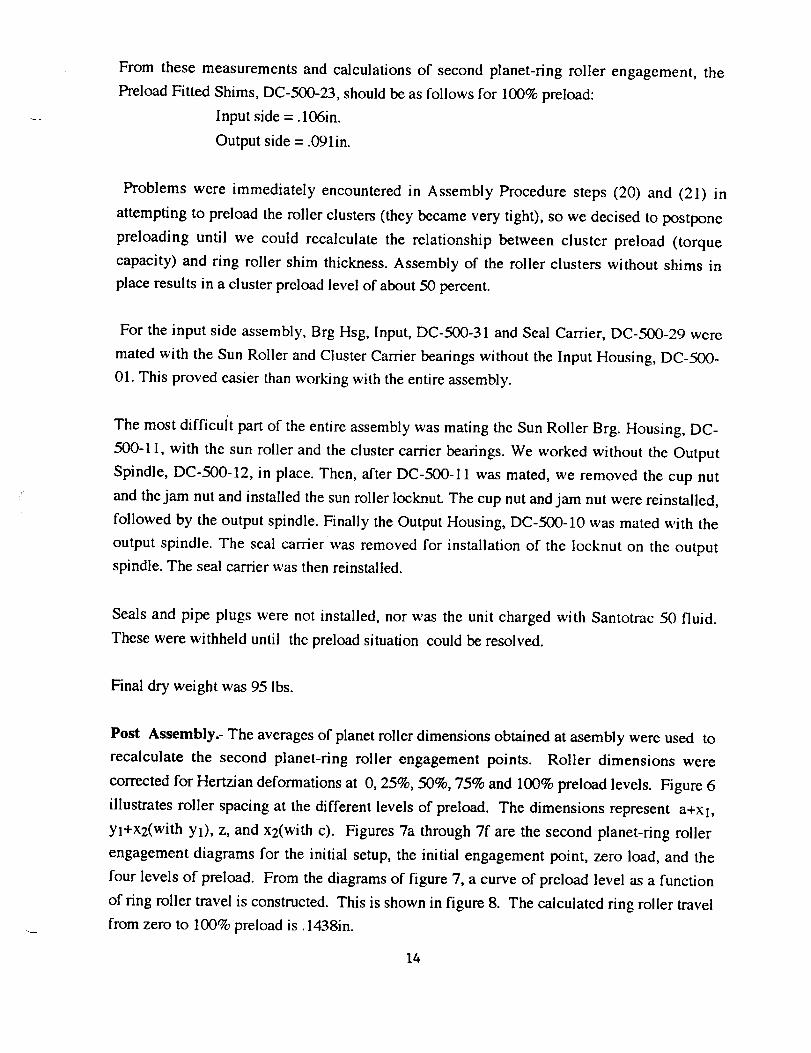
From thesemeasurementsand calculationsof secondplanet-ring roller engagement,thePreloadFitted Shims,DC-500-23,shouldbeasfollows for 100%preload:
Input side=. 106in.
Outputside= .091in.
Problemswere immediately encounteredin Assembly Proceduresteps (20) and (21) in
attemptingto preloadtheroller clusters(theybecamevery tight), so wedecisedto postpone
preloading until we could recalculate the relationship betweencluster preload (torquecapacity) and ring roller shim thickness.Assemblyof the roller clusterswithout shims inplaceresultsin a clusterpreloadlevelof about50percent.
For the input side assembly,Brg Hsg, Input, DC-500-31andSealCarrier,DC-500-29were
matedwith the SunRoller andClusterCarrierbearingswithout theInput Housing,DC-500-01.This provedeasierthanworkingwith theentireassembly.
The mostdifficul_tpartof theentireassemblywasmatingthe SunRoller Brg. Housing,DC-
500-11, with the sun roller and theclustercarrier bearings.We worked without the Output
Spindle,DC-500-12, in place.Then,after DC-500-11wasmated,we removedthe cup nutandthejam nutandinstalledthesunroller locknut.Thecupnutandjam nut werereinstalled,followed by theoutput spindle.Finally theOutputHousing,DC-500-10wasmatedwith the
output spindle.The seal carrier was removedfor installation of the locknut on the outputspindle.The sealcarrierwasthenreinstalled.
Sealsand pipe plugs were not installed,nor was the unit chargedwith Santotrac50 fluid.Thesewerewithheld until thepreloadsituation couldberesolved.
Final dry weight was95 lbs.
Post Assembly.- The averages of planet roller dimensions obtained at asembly were used to
recalculate the second planet-ring roller engagement points. Roller dimensions were
corrected for Hertzian deformations at 0, 25%, 50%, 75% and 100% preload levels. Figure 6
illustrates roller spacing at the different levels of preload. The dimensions represent a+xl,
yl+x2(with Yl), z, and x2(with c). Figures 7a through 7f are the second planet-ring roller
engagement diagrams for the initial setup, the initial engagement point, zero load, and the
four levels of preload. From the diagrams of figure 7, a curve of preload level as a function
of ring roller travel is constructed. This is shown in figure 8. The calculated ring roller travel
from zero to 100% preload is. 1438in.
14

The valuesof theX DIM for the inputandoutputsideclusters(given above)were thenused
together with the resultsof the engagementdiagramsto obtain curves of required shimthicknessvs. preload level. Theseareshownon figure 9 for the input side and output sideclusters. For 100%preloadthefollowing shimswouldbe required:
Input sideshim= .0738/.0838in.
Outputsideshim= .0588/.0688in.
For assemblywithout shimsthepreloadlevelsare:Input side= 30 to37%
Outputside= 45 to50%
As a compromiseto reducethedrive taretorqueslightly, thedrive wasassembledwith .060
in. shimson the input side and.045 in. shimson theoutput side. Theseshims produce apreloadlevel of approximately88%.Plasticshimstock with thicknessesof .005, .010, and
.015in. wasusedin theassembly.
It is quite probablethat taretorqueswoulddecreaseasthedrive is run in, but testingwouldbe requiredto verify that.
GROUNDED RING (MOMENTUM BALANCED) DRIVE (DC-400)
The conventional way to achieve dual counterrotating speed matched outputs from a single
input is to utilize a dual roller or roller-gear cluster arrangement [2]. One cluster has a non-
rotating cluster carrier or cage and rotating ring rollers, while the second cluster has non-
rotating ring rollers and a rotating cage. One output is taken from cluster 1 ring rollers, and
the second from cluster 2 cage. The two clusters are designed with ratios R and R+I to
achieve equal and opposite output speeds.
The Grounded Ring Drive represents a novel approach to achieving dual counterrotating
outputs with a significant reduction in size and weight (approximately 40%) as compared to
the conventional dual cluster design. The finalized geometric arrangement for the Grounded
Ring Drive is shown in figure 10. Outputs are taken from the rotating ring rollers and from
the rotating cage.The grounded ring is non-rotating and absorbs reaction torques which
depend in magnitude on the two output torques. Kinematic operation of the drive,
development of roller and gear geometries, key stress and deflection calculations, assembly
procedure, and inspection results at assembly will be discussed prior to discussion of test
results in a later section.
15

Kinematics
A complete kinematic development is given in [3]. To review briefly (see figure 11):
Cluster ratio: R = (c/y 1)(x l/a) (21)
If the two output speeds are equal and opposite, i.e., tOLl = - toL2. Then
_1 = -toH/(2R- 1)
toL2 = toII/(ER- 1)
To achieve a non-rotating grounded ring it is necessary that
Y2 = x2(c-x2)/(2c-x2) Then
c2 = c-x2+Y2
a2 = c2-2y2
where a2, Y2, and c2 are the grounded sun, planet, and ring radii.
A torque balance on the drive requires that:
TH + TEl - TL2 -/+ TGR = 0
When the drive is torque balanced:
TL1 - ((R- 1)/R)TL2
and
when
TL1 can be expressed as
From equations (27) and (29)
The input power to the drive is
TGR = 0
TLI = ((R-1)/R)TL2 it is shown in [3] that
TLI = ((R- 1)/R)TL2 +/- TGR
TH -(1- (R- 1)/R )TL2 = 0
Input power = THtoH
(22)
(23)
(24)
(25)
(26)
(27)
(28a)
(28b)
(29)
(30)
(31)
The output power from the drive is
Output power =TLItaLI + TL2toL2 (32)
The conclusion reached in [3] was that there would be phantom power loss when the output
torques are not in the ratio as given in equation (28a). A further examination of the torque
relationships as presented here shows that not to be the case. Neglecting friction losses, the
output power will always be equal to the input power, so there will be no loss in efficiency
due to phantom or recirculating power.
The DC-400 drive has a cluster ratio R=12.5 to achieve an input-output speed ratio (with
equal and opposite output speeds) of +/- 24. Regardless of the imbalance in output torques,
neglecting roller creep losses
16

mL2 = - COL2= C0H/2.A (33)
It should be noted that in the DC-400 drive the three shaft connections are kinematically
coupled so that none of the three can be constrained without constraining all three. This is in
contrast to the DC-700 and DC-500 drives, in both of which torque and motion transfer can
occur between any two shaft connections with the third shaft connection constrained or
locked. In the DC-400 drive torque and motion transfer between any two shaft connections
can only occur with the third connection free.
Cluster Geometry
Results of the computer program which sizes the rollers and establishes approximate cluster
geometry were presented in [3]. Table IX summarizes roller radii and, for the full output
torque conditions of 452Nm (4000inlbs.), normal forces, contact ellipse dimensions, Hertz
stresses and Hertz compressions for both the rotating (power transfer) and grounded ring
clusters. Hertz compressions are required to determine effective roller radii under load and
manufactured roller radii for desired preloading.
Stress and deflection analyses were done for the rotating cluster ring roller and the grounded
ring cluster sun and ring rollers. None of the other parts is subjected to stress levels that
require detailed stress analysis. As shown on ":able IX, the rotating cluster ring roller
maximum bending stress under full torque conditions is .148GPa (21,400 psi). That stress
level precludes the use of a through hardened alloy, so a case carburized steel is used. For the
grounded ring cluster, both the sun and ring roller bending stresses are very nominal ( on the
order of .0295 GPa (4,270 psi) so that the material chosen could be either through hardened
or case carburized. Sun and ring roller bending deflections are small ( on the order of
.005mm [.0002in.]), but were still factored into the manufactured radii.
Drawin2s
The Grounded Ring (Momentum Balanced) Drive is defined by assembly drawing DC-400.
The assembly drawing includes a listing of commercial parts as well as a listing of all
fabricated parts. Individual parts are detailed on drawings DC-400-01 through DC-400-36.
The roller drawings include coordinate tables for NC machining and metrology. Each of the
part drawings provides complete material and processing information necessary for
manufacture.
17
S"
Assembly
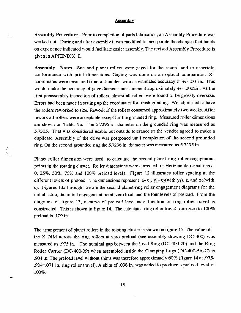
Assembly Procedure.- Prior to completion of parts fabrication, an Assembly Procedure was
worked out. During and after assembly it was modified to incorporate the changes that hands
on experience indicated would facilitate easier assembly. The revised Assembly Procedure is
given in APPENDIX E.
Assembly Notes.- Sun and planet rollers were gaged for the record and to ascertain
conformance with print dimensions. Gaging was done on an optical comparator. X-
coordinates were measured from a shoulder with an estimated accuracy of +/- .001in.. This
would make the accuracy of gage diameter measurement approximately +/- .0002in. At the
first preassembly inspection of rollers, almost all rollers were found to be grossly oversize.
Errors had been made in setting up the coordinates for finish grinding. We adjourned to have
the rollers reworked to size. Rework of the rollers consumed approximately two weeks. After
rework all rollers were acceptable except for the grounded ring. Measured roller dimensions
are shown on Table Xa. The 5.7296 in. diameter on the grounded ring was measured as
5.7305. That was considered usable but outside tolerance so the vendor agreed to make a
duplicate. Assembly of the drive was postponed until completion of the second grounded
ring. On the second grounded ring the 5.7296 in. diameter was measured as 5.7295 in.
Planet roller dimension were used to calculate the second planet-ring roller engagement
points in the rotating cluster. Roller dimensions were corrected for Hertzian deformations at
0, 25%, 50%, 75% and 100% preload levels. Figure 12 illustrates roller spacing at the
different levels of preload. The dimensions represent a+x 1, yl+x2(with Yl), z, and x2(with
c). Figures 13a through 13e are the second planet-ring roller engagement diagrams for the
initial setup, the initial engagement point, zero load, and the four levels of preload. From the
diagrams of figure 13, a curve of preload level as a function of ring roller travel is
constructed. This is shown in figure 14. The calculated ring roller travel from zero to 100%
preload is .109 in.
The arrangement of planet rollers in the rotating cluster is shown on figure 15. The value of
the X DIM across the ring rollers at zero preload (see assembly drawing DC-400) was
measured as .975 in. The nominal gap between the Load Ring (DC-400-20) and the Ring
Roller Carrier (DC-400-09) when assembled inside the Clamping Lugs (DC-400-5A-C) is
.904 in. The preload level without shims was therefore approximately 60% (figure 14 at .975-
.904=.071 in. ring roller travel). A shim of .038 in. was added to produce a preload level of
100%.
18

For the groundedring cluster, the value of the Y DIM acrossthe idler sun rollers at zero
preload(seeassemblydrawingDC-400)wasmeasuredas.747in. As shownon figure 16,the
nominal value is .7547 in. Figure 16 shows the initial engagementpoint and the final
engagementpoint at 100%preload.The idler sun rollers are3° conesso the contactpoints
betweenthemand theplanetshaftsremainsat the3° slopepoint on the 4.1 in. crossradiusp;anets.The idler sunrollersmustapproacheachotheratotal of .7547-.6792= .0755in. for
100%preload.The nominal shimrequiredis .679-(2*.250)= .179 in. For this assemblytheidler sun roller shimwasgroundto. 171in.
The parallelismof theaxesof thesecondrow plaaetshaftsand the drive axis is felt to be an
important parameter in the DC-400 drive. The z dimension in the cluster setups was
calculated using averages of the measured roller dimensions for the rotating and grounded
ring clusters.The calculated values were:
For the rotating cluster
For the grounded ring cluster
z= 2.393699 in.
z = 2.393475 in.
hz = .000224 in.
Within the accuracy of calculations, the axes should be parallel.
In assembling the cluster it was found that control of concentricity between the cluster carrier
axis and the roller cluster axis was critical. The inner output spindle must be fastened to the
cluster carrier before starting assembly of the roller cluster. When the ring rollers are in
place, the outer output spindle should be engaged with the ring roller carrier to insure that
concentricity between the roller cluster, cluster carrier and output spindles is not lost. The
assembly procedure was modified to incorporate these procedures.
Assembly was completed with the addition of 17 oz. of Santotrac 50 traction fluid.
Assembled weight was 58 lbs.
Post Assembly.- Breakaway torques were measured with deadweights applied to the input.
With both outputs free to rotate the tare torque was 8.65Nm (76.5 in-lbf). This torque is 24%
of the full torque rating of 36.17Nm (320in-lbf). The magnitude of the tare torque illustrates
the disadvantage of full preloading- high friction losses at low output torques.
A check of drive kinematics was conducted by rotating the input 25 revolutions. This
resulted in a 370 ° rotation (1.028 revolutions) of the inner output, and a 372 ° rotation (1.033
revolutions) of the outer output. These reduction ratios are 24.3 and 24.2. The calculated
19

cluster ratio is 12.5 or 24 with both outputs rotating equally and opposite, so the measured
ratios compare quite well with theory.
Post Failure Reassembly. Details of the failure which occurred shortly after the start of
tests are given under TEST RESULTS_ GROUNDED RING (MOMENTUM
BALANCED) DRIVE (DC-400). A new set of Planet Rollers, 1ST Row (DC-400-26) was
made, the alternate Grounded Ring (DC-400-03) replaced the Grounded Ring used in the first
asembly because the latter had a slightly scored roller track, and several other parts were
refurbished for the new assembly. Measurements of the new set of Planet Rollers, 1ST Row
are given on Table Xb. The X DIM was measured as .995 in. A ring roller shim of .015 in.
would have been required for 100% preload, but in view of the very high tare torque obtained
in the first assembly, it was decided to assemble with 80% preload, which required no
shimming. For the grounded ring cluster, grounded ring loading was recalculated with the
new grounded ring and the .171 in. idler sun roller shim used in the first assembly. It was
found to be 830 lbf (3,694N) which is very close to the 100% preload design value of 844 lbf
(3,756N). We then assembled with the. 171 in. idler sun roller shim. The new values of the
z dimension which determine parallelism between the drive axis and the axes of the second
row planet roller shafts were:
For the rotating cluster with 80% preload z= 2.393691 in.
For the grounded ring cluster z = 2.393975 in.
Az= - .003284 in.
As for the first assembly, within the accuracy of calculations, the axes should be parallel.
As with the first assembly, breakaway torque was measured with deadweights applied to the
input. With both outputs free to rotate the tare torque was 1.36Nm (12 in-lbf). This torque is
3.8% of the full torque rating of 36.17Nm (320in-lbf), and is significantly lower than that
obtained in the first assembly. This indicates that there may have been several faults in the
first assembly.
A check of drive kinematics was conducted by rotating the input 24 revolutions. This
resulted in exactly 360 ° rotation (1 revolution) of both the inner and outer outputs (within
the accuracy of measurement). The drive seemed very smooth with little or no perceptible
cogging.
20

TEST FACILITY
A test facility capable of applying and reacting torques, and of accurately measuring torques,
angular shaft positions, and rotational speeds was designed to evaluate the performance
characteristics of all three drives. The instrumentation incorporated in the test facility made
possible measurement of angular and torque ripple, viscous and Coulomb friction, and
forward and reverse power efficiency. The arrangement of components is shown quarter
scale on drawings DC-800 SK, sheet 1 for the differential drives and sheet 2 for the
momentum balanced drive. Fabricated parts for the test facility are defined by drawings DC-
800-01 through DC-800-29. These are listed, together with major commercial parts, on
drawing DC-800 SK sheet 1. Schematics of the component arrangements are shown in
figure 17a for the differential drives and in figure 17b for the momentum balanced drive.
Figure 18 shows photos of the test setups.
A notably challenging aspect of the test stand design was the need to drive concentric inputs
(or outputs). To do so, it was necessary to utilize a hollow drive shaft, torque transducer,
torque motor, and encoder for the outer shaft. Limited space for coaxial shafts made some
compromises in angular stiffness necessary.
Components used in the test stand included: three drive motors, three torque transducers, 3
precision encoders, a load transmission, a multiprocessor motor control and data acquisition
system, and a variety of mechanical fixtures.
MOTORS
The most important components in the test stand were the drive motors used to power the
transmissions. The drive motors included two Compumotor KHX-740 ac servo motors and
one Uniq Mobility SR-180 brushless dc motor. For the DC-700 and DC-500 transmission
tests the Compumotor electronic drives were modified such that the motors could be operated
in three different modes: linear PD servo feedback, torque-controlled mode, or synchronous
mode. These motors were capable of providing the full 19 N-m (170 in-lbf) desired "input"
(high-speed) torque, but were limited in speed to approximately 135 rad/sec (1300 rpm).
These motors were capable of both supplying and absorbing power up to these torque and
speed limits. Because of the Compumotors' speed limitations, the maximum power these
motors could source or sink was limited to approximately 2.5kW. Thus, the DC-700 and DC-
500 transmission tests were primarily limited to roughly half the transmissions' rated speed
and power (except for limited cases in which both Compumotors acted as maximum power
21

sinks).
The third drive motor, the Uniq Mobility SR-180, was required for its relatively rare quality
of offering a hollow armature. This design permitted driving the outer shaft of each of the
transmissions. The inner shaft of each transmission was driven via a shaft extension, which
passed through the center of the Uniq motor, as well as its associated torque sensor and
encoder. The Uniq motor was much more powerful than the Compumotors. It was capable
of no-load speeds up to 570 rad/sec (5450 rpm), intermittent low-speed torque up to 34 N-m
(300 in-lbf), and intermittent power up to 12kW (16hp). The associated controller was built
for full 4-quadrant operation, with regeneration to zero speed. The higher speed, torque and
power capabilities of the Uniq motor were exploited under conditions for which both
Compumotors were running at full speed and power. The Uniq motor was able to balance
double the speed of the two Compumotors and was able to balance the combined power of
the two Compumotors. Under this condition only, full rated speed and power of the DC-700
and DC-500 transmissions were tested.
A limitation of the Uniq motor was its inability to provide well-regulated power absorption
and its poor controllability at low speeds. This motor was capable of regenerating power
down to low speeds, as specified. However, the power absorption occurred in sharp
pulsations, making it unusable as a precision power sink for efficiency tests. As a result, the
Uniq motor was always used as a power source for all efficiency tests of the DC-700 and
DC-500 transmissions. For the DC-400 transmission, it was used primarily as a power source
for efficiency tests, though some limited testing was conducted with this motor acting as a
power sink. The consequence of this limitation for the DC-400 tests was that efficiency data
was taken primarily with the transmission acting as a speed increaser rather than the more
normal sped reducer mode.
It was also observed that the Uniq motor did not provide smooth torque production at speeds
below about 35 rad/sec (335rpm). Thus, efficiency tests did not include cases for which
transmission shaft H2 (outer input shaft of DC-700 and DC-500) ran at speeds less than 35
rad/sec. This restriction included zero speed, as the Uniq motor could not servo to a fixed
angle.
Yet another limitation of the Uniq motor was its inability to interface to computer controls.
Although the logic power supply of the Uniq driver was described as decoupled from the
motor drive power, the electronic controls were not compatible with computer outputs. This
problem could be solved using analog isolator modules, though this should not have been
necessary. Ultimately, the Uniq motor was controlled manually via the control pendant
22

providedby the motor manufacturer.The Compumotorswere controlled by the computer,
andfinal load adjustmentsweremademanuallywith theUniq motor.
Synchronous-modecontrol of theCompumotorswasusedalmostexclusively in the testsoftheDC-700and DC-500 transmissions.This controlmodeenabledprecisespeedregulation
of two of thethreeshaftsof eachtransmission.TheUniq motor wasusedasa torquesource.
In fact, the control interfaceavailablefor the Uniq motor wasa velocity command,which
would seemto be in conflict with velocity control of the two Compumotors. However, theUniq motor controller utilized a weak,proportional-onlyvelocity-error feedbackcontrollerinternal to the poweramplifier to regulatemotor torque. As a result, the Uniq motor, under
load, would not achieve its commanded velocity. Rather, the velocity-controlled
Compumotorswould constrainthespeedof theUniq motor. Velocity commandsto theUniq
motorhigherthan theshaftvelocity imposedby theCompumotorsresultedin a velocity error
in the Uniq controller, resulting in a proportional torque response. As a result, the Uniq
motor could be utilized as a torque source by varying its velocity command. TheCompumotorsrespondedaccordinglyto reactto thetorqueintroducedby theUniq motor, butsynchronouscontrolof the Compumotorsmaintaineda regulatedspeed.In this manner,it
was possibleto establishvariouscombinationsof shaft speedsand torques, subject to the
restrictions noted on maximum speedsof the Compumotorsand the requirement that theUniq motor actasa powersource.
For the DC-400 tests the Compumotors were driven in two different modes. The
Compumotordriving theinputshaft(shaftH) wasdriven in synchronousmode.Synchronous
modecontrol enabledpreciseregulationof input speeds.Sincethe low speedshafts(L1 and
L2) were dependenton the input speed,themotorson shaftsL1 and L2 wcre controlled astorquesources,notasspeedsources.
For the DC-400 transmissiontests,utilizing the Uniq motor as a torque source involved
depending on its relatively Hsoft"velocity servo stiffness. Since the velocity-controlled
Compumotor constrained the speedof the Uniq motor (within torque limits of the
Compumotor), the speedof shaft H was precisely regulated,and the speedof shaft L2
followed by kinematicconstraint Velocity commandsto theUniq motor higher than theL2shaft velocity resulted in a velocity error in the Uniq controller, inducing a proportional
torque response. In this manner,the Uniq motor could be utilized as a torque sourceby
varying its velocity commandslightlyaboveor belowtheregulatedvelocity of shaftL2.
The Compumotor on shaft L1 was also torque controlled. As the torque of shaft L2 (Uniq
motor torque) was adjusted, the torque on shaft L1 was adjusted as well, to keep the two
23

output torques relatively close. Most desirable operation of the DC-400 drive occurs when the
outputtorques are kept comparable--within approximately 30% of each other.
By varying the velocity of shaft H, the torque load on shaft L1 and the torque load on shaft
L2, the space of valid loading conditions could be evaluated.
TEST STAND GEARING
For the DC-700 and DC-500 tests, the motors used were appropriately sized for direct drive
of the high-speed transmission shafts. However, to source or sink power at the low-speed
shaft(s), it was necessary to reduce the speed and increase the torque of the motors. Two
additional transmissions were used for this.
For the single low-speed shaft L of transmissions DC-700 and DC-500, a Nastec model
NAS-300A transmission was used. This transmission had a ratio of 29.23: 1, and exceeded
the torque, speed and power ratings of the DC-series transmissions under test.The 29.23:1
ratio was a good match for the 29.23:1 and 24:1 ratios of transmissions under test. In all
cases, the NAS-300A transmission was driven by a Compumotor at its high-speed shaft, and
the low-speed shaft was connected in series with a 2804T (4-3) Himmelstein reactionless
torque meter (Figure 17). Both input and output shafts of the NAS-300A were coupled via
Thomas flexible couplings. Due to its high linearity, low friction and good efficiency as
both a speed reducer and speed increaser, the NAS-300A transmission was well suited for
performing as a component within both a power source and a power sink.
For the DC-400 transmission tests the Compumotor used for shaft H was under-sized for
direct drive of this high-speed shaft. Neither the maximum speed nor the maximum torque of
the Compumotor could attain the rated limits of the DC-400 input shaft. However, the speed
and torque limits of the Compumotor were reasonably balanced with respect to the DC-400
constraints, and thus direct drive of shaft H was preferable to the addition of an input
transmission.
Shafts Ll(inner output) and L2(outer output) of DC-400, on the other hand, called for torque
loading far in excess of that which could be supplied by the motors, albeit at a much lower
speed. To match the electromechanical drives to the task, load transmissions were required.
For shaft L1 of DC-400, a Nastec model NAS-300A transmission was used. This
24

transmission exceededthe torque,speedand power ratings of the DC-400 transmission
under test. The 29.23:1 ratio was a reasonable match for the (nominal) 24:1 ratio of the DC-
400. The NAS-300A transmission was driven by a Compumotor at its high-speed shaft, and
the low-speed shaft was connected in series with a 2804T (4-3) Himmelstein reactionless
torque meter. Both input and output shafts of the NAS-300A were coupled via Thomas
flexible couplings. The NAS-300A transmission was well suited for performing as a
component within both a power source and a power sink.
For shaft L2 of DC-400, a second speed reducer was needed. A constraint on this
transmission was that it had to permit torque measurements of the outer output shaft (shaft
L2) while providing a through hole for passage of the inner output shaft (shaft L1) extension.
A harmonic drive, Harmonic Drive model HDC-8M with a 60:1 ratio was used for this. The
ratio of 60:1 was not as well matched as the 29.23:1 NAS-300A transmission, but the higher
speed range of the Uniq motor, with which the harmonic drive was used, made the harmonic
drive a viable candidate.
In practice, the harmonic drive presented a more severe limitation than expected. When the
harmonic drive's wave generator was driven in excess of approximately 3,000 rpm, the wave
generator was not stable. At these speeds, the wave generator would "walk" axially along the
concentric shaft L1, and would bind against components it contacted. Consequently,
measurements were restricted to input speeds between plus and minus 105 rad/sec
(approximately 1,000 rpm), corresponding to approximately 262 rad/sec (2,500 rpm) of shaft
L2. This speed restriction further limited the range of data (both speed and power) that could
be measured.
TORQUE SENSORS
Torque measurements were performed using Himmelstein torque meters. Each torque meter
had been calibrated at the factory, and is nominally rated for 0.1% linearity and hysteresis.
Compatible Himmelstein torque-meter signal conditioners (model 6-201) were used.
For each transmission, two reactionless rotating torque meters and one reaction-type torque
meter were used. Reactionless torque meter Himmelstein model 2402T (35-1), with a full-
scale range of 40N-m (350 in-lbf), was used in each case to measure a high-speed shaft
torque of transmissions DC-700 and DC-500. The range of this torque meter was
25

approximately twice the rated input torque of each of the transmissions. This meter was
connected in series with a Compumotor and shaft H1 using Thomas flexible couplings.
Torques could be measured with this meter while the shaft was rotating, and the meter
introduced no perceptible additional torque loading. However, this type of meter uses a solid
shaft, which does not accommodate concentric differential shafts. Thus, torques from shaft
H2 of DC-700 and DC-500 could not be measured with this type of meter.
Low-speed shaft torques (shaft L of DC-700 and DC-500) were measured using Himmelstein
reactionless torque meter model 2804T (4-3). This meter had a full-scale output of 450 N-m
(4,000 in-lbf). This capacity matched the output rating of the transmissions, and was thus
optimally ranged for highest precision. The meter was connected in series between the low-
speed, high-torque shaft L, and a torque load (a geared-down Compumotor) using Thomas
flexible couplings.
The third torque, in each case, applied to the outer input shaft of the dual, concentric shafts of
DC-700 and DC-500, was measured using a reaction-type torque meter. For these
transmissions, torque was provided to shaft H2 from direct drive of the Uniq motor. The
applied torque was measured using Himmelstein reaction torque meter model 2030 (6-2),
with a range of 68 N-m (600 in-lbf). The range of this meter was not optimal for the
application, since the span was 350% of the torque range to be applied. This meter did,
however, provide the required through-hole dimensions. In addition, it could adequately
support the cantilever moment produced by the 21 Kg (47ibm) Uniq motor. The reaction
torque meter was bolted on one side to the case of the DC-700 or DC-500 transmission, and
the other flange was bolted to the stator of the Uniq motor. The Uniq motor was not
supported by any other means. Thus, rotor torques from the Uniq motor reacted equal and
opposite on the stator, which was supported solely by the reaction torque meter. By this
arrangment, torques applied to shaft H2 could be measured accurately with a non-rotating
torque transducer, and this construction allowed for unimpeded passage of a shaft extension
from shaft H1.As stated the range of the model 2030 (6-2) meter was suboptimal, being
350% higher than the desired measurement span. Consequently, there was some compromise
of precision in measuring the torques of interest in the DC-700 and DC-500 tests.
For the DC-400 tests, a reactionless torque meter Himmelstein model 2402T (35-1), with a
full-scale range of 40N-m (350 in-lbf), was used to measure high-speed shaft torque (H).
The range of this torque meter was well matched to the rated input torque of the DC-400,
although the Compumotor drive was not capable of producing torques to this torque level.
This reactionless torque meter was connected in series between a Compumotor and shaft H
using Thomas flexible couplings.
26

Low-speedshaft torques(shaftsL1 andL2 of DC-400)weremeasuredusingonereactionless
torque meter and one reaction-typetorquemeter. Himmelsteinreactionlesstorque meter
model 2804T (4-3), with a full-scaleoutputof 450 N-m (4,000in-lb), waswell matchedtothetorque rangeof theoutputshafts,but, dueto thismeter'ssolid shaft, its usewas restricted
to shaftL1. This meterwasinstalledbetweenshaftL1 of DC-400andthe high-torque/low-speedshaft of the NAS-3OOA load transmission using Thomas flexible couplings with
keyways.
The third torque of DC-400, that of shaft L2, was measured using a reaction-type torque
meter. A Himmelstein model 2060 (1-4) reaction-type torque meter, with a range of 1,130
N-m (10,000 in-lbf), was bolted on one side to the case of the DC-400 transmission. The
drive package for shaft L2 (consisting of the harmonic-drive transmission coupled to the
Uniq motor) was bolted to the other flange of the torque meter. No other supporting structure
was provided for the motor/harmonic drive. Thus, all torques from shaft L2 reacted through
the reaction torque meter to the case of the transmission. Although there were frictional
losses in both the motor and speed reducer, these losses acted only as intemal moments. The
net torque acting on shaft L2 was accurately sensed via its reaction torque with respect to the
transmission case, independent of internal losses in the electromechanical drive package.
The range of the model 2060 (I-4) meter was suboptimal, being 250% higher than the DC-
400 transmission's rated maximum torque output. (The torque range oversizing was worse
still with respect to the torques which could be achieved in the tests). Consequently, there
was some compromise of precision in measuring the torques of interest in the DC-400 tests.
Use of this torquemeter was nonetheless necessary, due to the large cantilever loads it was
required to support as well as the relatively large axial through-hole required.
ANGULAR POSITION SENSORS
For measuring transmission ratio linearity, high-precision encoders were used. For the inner
input shaft and output shaft of DC-700 and DC-500 (shafts H1 and L), identical encoders,
BEI series 143, were used. These solid-shaft encoders provided 360,000 counts per
revolution, offering a resolution of 6.28 mrad (0.001 deg). For the third shaft (H2) of the
DC-700 and DC-500 transmissions, an angular sensor with a through hole was required. A
similar BEI encoder, model 5VL677, also with 360,000 counts per revolution, was acquired
for this purpose. This encoder provided a hollow shaft with a 2-inch bore.
27

A design modification from the original plan was required to use the hollow-shaft BEI
encoder. The mount between this encoder and the Uniq motor did not originally incorporate a
flexible coupling. Since the Uniq motor was cantilevered from a reaction-type torque meter,
its mount had significant flexibility. The resulting misalignment with respect to the rigid
coupling of the encoder made the encoder unusable. A coupling modification was made, in
which the outer spline to shaft H2 (part numbers DC-800-10 and DC-800-18 for the DC-700
and DC-500 drives, respectively) was mated to a modified Thomas flexible coupling. The
other side of this coupling was modified to fit the interface flange (part number DC-800-23)
of the BEI encoder. A consequence of this modification was that the Uniq motor had to be
removed to install the hollow-shaft BEI encoder. However, this was not a limitation for the
linearity or cogging tests, since under these tests, the input shaft was rotated manually.
In the DC-400 tests, for shafts H and L1, BEI encoders, series 143, were used. For shaft L2,
the BEI encoder, model 5VL677, also with 360,000 counts per revolution, was used. This
encoder provided a hollow shaft with a 2-inch bore.
The high-precision encoders were used only in low-speed, manually-driven torque-tipple and
angular linearity tests. For all motor-driven tests, only velocities (not high-precision angles)
were needed. For friction and efficiency tests, velocities were known from the drive
frequency in synchronous mode, and these velocities were verified using lower-resolution,
higher-speed encoders on the Compumotors.
For linearity tests, the load transmissions were removed, and the encoders were coupled
directly to shafts. This enabled precision angular measurements unaffected by imperfections
of the load transmissions.
MECHANICAL COUPLINGS
Most mechanical couplings for rotating parts used Thomas flexible couplings. These
couplings accommodate minor shaft misalignments, both translational and rotational, yet are
stiff and backlash free in torsion. In most instances, the Thomas couplings were coupled to
shafts using Fenner-Manheim "Trantorque" friction/expansion couplings. Couplings made
with the Trantorques were stiff and backlash free.
28
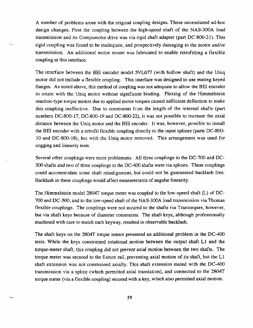
A numberof problemsarosewith the original couplingdesigns.Thesenecessitatedad-hoc
designchanges.First the coupling betweenthe high-speed shaft of the NAS-300A load
transmission and its Compumotor drive was via rigid shaft adapter (part DC-800-21). This
rigid coupling was found to be inadequate, and prospectively damaging to the motor and/or
transmission. An additional motor mount was fabricated to enable retrofitting a flexible
coupling at this interface.
The interface between the BEI encoder model 5VL677 (with hollow shaft) and the Uniq
motor did not include a flexible coupling. This interface was designed to use mating keyed
flanges. As noted above, this method of coupling was not adequate to allow the BEI encoder
to rotate with the Uniq motor without significznt binding. Flexing of the Himmelstein
reaction-type torque meters due to applied motor torques caused sufficient deflection to make
this coupling ineffective. Due to constraints from the length of the internal shafts (part
numbers DC-800-17, DC-800-19 and DC-800-22), it was not possible to increase the axial
distance between the Uniq motor and the BEI encoder. It was, however, possible to install
the BEI encoder with a retrofit flexible coupling directly to the input splines (parts DC-800-
10 and DC-800-18), but with the Uniq motor removed. This arrangement was used for
cogging and linearity tests.
Several other couplings were more problematic. All three couplings to the DC-700 and DC-
500 shafts and two of three couplings to the DC-400 shafts were via splines. These couplings
could accommodate some shaft misalignment, but could not be guaranteed backlash free.
Backlash in these couplings would affect measurements of angular linearity.
The Himmelstein model 2804T torque meter was coupled to the low-speed shaft (L) of DC-
700 and DC-500, and to the low-speed shaft of the NAS-300A load transmission via Thomas
flexible couplings. The couplings were not secured to the shafts via Trantorques, however,
but via shaft keys because of diameter constraints. The shaft keys, although professionally
machined with care to match each keyway, resulted in observable backlash.
The shaft keys on the 2804T torque sensor presented an additional problem in the DC-400
tests. While the keys constrained rotational motion between the output shaft L1 and the
torque-meter shaft, this coupling did not prevent axial motion between the two shafts. The
torque meter was secured to the fixture rail, preventing axial motion of its shaft, but the L1
shaft extension was not constrained axially. This shaft extension mated with the DC-400
transmission via a spline (which permitted axial translation), and connected to the 2804T
torque meter (via a flexible coupling) secured with a key, which also permitted axial motion.
29

The axial freedom of the L1 shaftextensionof DC-400becamea problem, since this shaft
was responsiblefor constrainingaxial motion of the flex splineof the harmonicdrive (via
thrustwasherson theL1 shaftextension).Theflex splineproducedunexpectedlylargeaxialforceson the thrust washersof the L1 shaft extension. Consequently,the shaft extension
would translateaxially until theflex splinecamein contactwith theUniq motor housing(ononeside)or producedexcessivefrictional torqueson theinnershaft(via the thrustwasherontheotherside).This designflaw in theteststandmadedatacollection difficult. Datacould
be acquired for relatively short durations,until the LI shaft extensiondisplaced too far
axially and had to be re-adjusted. When the flex splinedisplacedaway from the DC-400transmission,suchdisplacementcouldbenotedvisuallyandthe testwould be halted. When
theflex splinedisplacedtowardstheDC-400,however,significant frictional torquesbetweenL2 andL1 could develop,andthis conditionwasnot visuallyobvious. Underconditions of
suchinternal binding, the lossesareindistinguishablefrom efficiency lossesinternal to theDC-400.
Finally, the mechanicalcoupling securingthe wave generatorof the harmonic drive also
provedto be inadequate.Thewavegeneratorwasdrivenby theUniq motor via a spline. As
with the L1 shaft extender,however,no axial constraintwasprovided. Consequently,thewave generatorwas capableof translatingaxially under operation. This unconstrained
motion wasparticularlyproblematicat higherspeeds,limiting thetop speedat which theDC-400could betested.
For theangularlinearity measurements,the2804Ttorquemeterandits keyedshaftcouplingswereremoved,so asnot to influencethe measurements.However, the shaft connectionto
the output (e.g., part DC-800-20,output shaft for the DC-700and DC-500 drives) had a
mating spline on oneend,anda keywayon theother. Backlashassociatedwith the key of
this requiredpartwasproblematicfor angularlinearitymeasurements.
For linearity and torque-rippletestsof DC-700and DC-500,one shaft at a time was fixed
stationary,one shaft was rotated,andthe input torqueof the driven shaft and anglesof thedriven and free shaftsweremeasured.To secureoneshaft at a time, the chosenshaft wascoupledvia aTrantorqueto a stiff fixture boltedto therail.
For the DC-400 testsit was not permissibleto fix or constrainany of the threeshafts.To
minimize theinfluenceof systembacklashon linearitymeasurements,oneshaftat a time was
rotatedslowly and smoothly (manually)without direction reversalswithin a given test. By
rotating in a constantdirection,and by avoiding inertial effects,any backlashin the system
30

shouldhave approachedandremainedin contactwith its limit. Thus, backlasheffectswould
be removedfrom thelinearity tests.
In retrospect,the test-standdesignshouldhave:1)eliminatedall keyway couplings in favor
of backlash-freecouplingssuchasTrantorques( spatialconstraintsdid not permit thoseto beused); 2) provided axial thrust bearingsfor the flexible spline of the harmonic drive; 3)
provided thrust bearingsrestrainingaxial motion of the harmonicdrive's wave generator.
All otherdesignfeaturesof theteststandwerefoundto besuccessful.
Eachcomponentof thesystemwasmountedto acommonrail (a 2-piece,10'aluminum I-
beam,bolted to aconcretefloor) usingcustommountingfixtures( drawing DC-800,sheets1and2, andfigure 17). Thefixtures locatedall shaftcentersnominally 19.05cm (7.5") abovetherail.
EXPERIMENTAL PRECISION
An2ular Position Measurements.
The resolution of the encoders was plus or minus 6.28 mrad (0.001 deg). Transmission ratios
were measured incrementally, reported in terms of change of input angle divided by change
in output angle, fixing one shaft at a time. Measurements were recorded every 1 degree of
output rotation. For high-speed to low-speed shaft measurements, error associated with the
encoder resolution can be calculated. For a nominal transmission ratio of 24:1, plus or minus
one increment of the output and input encoders would result in apparent ratios of 24.025:1
and 23.975:1, or 0.1% error. For a nominal ratio of 1:1 (e.g., the ratio between dual inputs
or dual outputs), the error associated with encoder resolution is 0.2%, based on 1-degree
angular changes.
A potentially more significant error was due to backlash in the spline couplings to the
transmission, (e.g., part DC-800-20) and (more prominently) their associated keys/keyways.
To attempt to remove this effect from the measurements, rotations were induced
continuously in first the positive direction for one full output revolution, then in the negative
direction for a full revolution. This approach should minimize the effects of backlash in the
external couplings, but would also disguise any backlash internal to the transmission. Under
the circumstances, backlash of the transmission could not be measured reliably, but linearity
of transmission ratios should be trustworthy to within approximately 0.2%.
31

Torque Measurements
The torque meters were calibrated by Himmelstein, and claimed traceable to NIST standards.
The stated precision (linearity and hysteresis) is 0.2% (0.1% each) of full scale. Voltages
were sampled using a 12-bit, ADC, with a span of -5V to +5V, resulting in a conversion
accuracy (plus or minus one bit) of 0.05%.
The Himmelstein models 2402T (35-1) and 2030 (6-1), with 350 in-lbf and 600 in-lbf ranges,
respectively, were coupled in series, torques were applied, and the readings were recorded
from each. At 300 in-ibf load, the two meters agreed within 0.8 in-ibf. This variance falls
within the claimed tolerance of 0.1% full scale, allowing for 0.6 in-lbf error from the 2030
meter and 0.35 in-lbf error from the 2402T meter. At lower torques, however, the
discrepancy between the two meters was as high as 2.2 in-lbf (worst case, at 221 in-lbf
applied torque). Such a discrepancy would translate into an efficiency error of plus or minus
1%. The discrepancy at 170 in-lbf, the rated input torque, was 2.0 in-lbf, which would
produce a 1.2% error in computed efficiencies.
The high-torque meter (2804T at 4,000 in-lbf range) could not be compared directly to the
lower torque meters, as their ranges were so disparate. However, this meter is a scaled up
design of the 2402T, is made by the same manufacturer, is claimed to have the same relative
precision, and was used used with the same signal conditioning electronics. This high-torque
meter was well scaled to its application. The two low-torque meters, 2402T and 2030, were
oversized by 200% and 350%, respectively, whereas the high-torque meter (2804T) was
scaled to the correct 100% full range. We may thus reasonably estimate that the output meter
would introduce errors comparable to (or lower than) those observed with the relative
readings of the low-torque meters. With three meters in operation, efficiency measurements
should be within plus or minus 2.5%, as a conservative worst case.
In measuring the output torques of the DC-400 transmission, similar, but larger torque meters
were used. Himmelstein model 2060 (1-4) reaction-type torque meter, with a range of 1,130
N-m (10,000 in-lbf) was used to measure the outer-ring (L2) torque. Himmelstein
reactionless torque meter model 2804T (4-3) with a full-scale output of 450 N-m (4,000 in-
lb) was used to measure the inner output torque (L1). These two meters were not compared
directly in series, but since they had the same manufacturer, same construction type and
roughly the same ratio of torque ranges as the lower-range meter pair, comparable precision
limits may be expected.
32
Calibrating the high-torquemeters(2060at 10,000in-lbf range, and 2804T at 4,000 in-lbf
range) with respect to the input torque meter (2402T, 350in-lbf) was impractical, due to the
disparity in ranges. The manufacturer's calibration numbers had to be trusted. Given that all
meters used were fabricated and calibrated by the same manufacturer, that the meters were
quoted to have the same relative precision, and that all meters were used with identical
signal-processing electronics, the relative errors in calibration among the meters may be
presumed to be within the quoted tolerances, as confirmed by tests on the lower-range
meters. With three meters in operation, efficiency measurements should be within plus or
minus 2.5%, as a conservative worst case.
Another source of error in the torque measurements was electrical noise. Although the signal
conditioning electronics incorporated modulation noise-suppresion techniques, the
substantial electromagnetic interference produced by the switching amplifiers of the three
motors did produce a noticeable bias of noise on the torque signals. With the motors on, a
bias of 57mV was observed, which corresponds to just over 1% full scale. Powering the
signal conditioners from an isolated line-power supply seemed to improve, but not eliminate
the problem. Subsequently, the noise-induced bias torque was accounted for by assuming
symmetry of the transmission behavior at positive and negative velocities. Asymmetries,
assumed induced by torque-sensor noise, were removed mathematically in post-processing
the data.
Finally, another source of error peculiar to the 2804T meter is possible sensor saturation.
The torque meters are safe to operate up to twice their rated output. However, the analog-to-
digital converter used saturated at 5V input, corresponding to the full-scale rating of each
meter. Since the 2804T meter was rated for 4,000 in-lbf, matching the output rating of the
transmissions, tests which slightly exceeded this torque would be incorrectly recorded as
equalling this torque. Data with output torques very close to 4,000 in-lbf may, therefore, not
be reliable.
Velocity Measurements
Velocities were regulated by driving the Compumotors in synchronous mode. This produced
the equivalent of electronic gearing, for which the number of mechanical revolutions per
electrical revolution is a fixed integer. As a result, as long as the motors maintained
synchronism, the speed was (on the average) precisely the same as the drive frequency. Loss
of synchronism was obvious, as the motors would stall.
33

In the DC-700 and DC-500 tests two of the three motors were driven in synchronous mode.
The velocity of the third (the Uniq motor) could be precisely inferred from the known
(measured) transmission ratio. For efficiency computations, error associated with velocity
measurements was insignificant relative to other sources of error.
In the DC-400 tests only the input motor (shaft H) was driven in synchronous mode. The
velocity of the output shafts could be inferred from the known (measured) transmission ratio.
The velocity of shaft L1 was measured nonetheless via an encoder on the Compumotor
driving the load transmission NAS-300A. Since this load transmission had a precise gear
ratio fixed by gear teeth, the speed of shaft L1 (coupled to the low-speed output of the NAS-
300A transmission) could be accurately deduced. Measurements showed that the
transmission ratio of the DC-400 was not constant. Under varying load, the speed ratio from
shaft H to shaft L1 changed, due to roller creep. The speed of shaft L1 changed by
approximately 2% as the torque increased from zero to 2,000 in-lbf. It is presumed that shaft
L2 experienced comparable speed changes under load, though this could not be measured
directly.
In the analyses of efficiency of DC-400, it is presumed that the speed of shaft I_,2 is equal to
the measured speed of shaft LI, since the torques on L1 and L2 were comparable. This
assumption should correct for the expected (but unmeasured) speed variations of shaft L2,
making error associated with velocity measurements insignificant relative to other sources of
error.
INFLUENCE OF RESONANCES
Mechanical resonances were observed during testing. For example, for the DC-700
transmission, one such resonance was near 35 rad/sec input speed, which corresponded to
one of the chosen velocity states. Resonances can produce fluctuating torques and velocities.
Since the data acquisition averaged torque and velocities measurements, it did not account for
possible phase differences between fluctuating signals (analogous to a power factor in
reactive electrical systems). Average velocity and torque measurements under resonant
conditions are correctly reported, but efficiency computations for data taken under resonant
conditions may not be reliable.
Resonances observed could not be attributed to the transmissions themselves. Compliances
of the flexible couplings, flexing of the aluminum rail, and magnetic cogging of the motors
all contribute to the system dynamics, making transmission effects impossible to isolate
under the test conditions.
34

TEST RESULTS
DUAL INPUT DIFFERENTIAL ROLLER-GEAR DRIVE (DC-700)
The DC-700 transmission was integrated into the test stand as per drawing DC-800-SK,
subject to the coupling modifications noted earlier. Angular linearity, torque cogging,
Coulomb and viscous friction, and power transfer efficiency were measured. Test
procedures, data, and interpretation for the DC-700 drive are presented in this section.
Before presenting the data, a note on sign conventions is important. All rotations have been
defined as positive pointing out of the transmission. A positive rotation of H1 produces a
negative rotation of L, and a positive rotation of H2 produces a positive rotation of L. If H1
and H2 both rotate at the same speed in the same direction, then shaft L remains stationary.
The formula for relating the shaft velocities (previously presented as eq. (7) is:
o_L = OJH2/R2L - OJH1/R1L (34)
where taL is the angular velocity of shaft L, O_Hl is the angular velocity of shaft H1 and OJH2is
the angular velocity of shaft H2. The ratios R1L and R2L are the transmission ratios from
shaft HI to L and from shaft H2 to L, respectively. As will be shown from the data, R1L =
R2L = 29.23 for the DC-700 transmission.
Ideally, torque production in the DC-700 drive could be computed as:
17=, -R2L'ITH2 + R1L'I;H1 (35)
Since R1L = R2L for the DC-700, the input torques would, ideally, always be equal and
opposite. Any torque imbalance between the H1 and H2 shafts would result in acceleration
of the transmission until the balance condition is met. Note, though, that while the input
torques should balance, there is no such constraint on the input velocities. The input torques
are more nearly balanced when the input shafts deliver nearly equal power.
The torque signs have been assigned such that positive torque and positive velocity at any
shaft implies power flow into the transmission at that shaft. The DC-700 was tested with
power flows both into and out of shafts H1 and L. Since the Uniq motor was not a well-
controlled power sink, shaft H2 was always driven with power in.
35

Anmalarity Linearl W
On the average, a geared transmission has a precise, integer-fraction transmission ratio, as
dictated by tooth ratios. Within a revolution, however, there are small variations in the ratio
of incremental input angle to incremental output angle. Such variations give rise to velocity
ripple of the output for smooth rotation of the input. Velocity ripple acting on a load inertia
induces torque pulsations. Transmissions with identical reduction ratios can have quite
different dynamic behaviors within a system, depending on the linearity.
Linearity Test Procedure.- Linearity was measured with the high-precision BEI encoders
on shafts H1 and L, while shaft H2 was clamped still. The input shaft, H1, was rotated slowly
by hand while the computer continuously polled the encoder angles. For each 1.000-deg
increment of the output (shaft L), the input angle was sampled and the incremental ratio was
computed.
These tests were performed with constant positive or constant negative rotation of the driven
shaft, so as to minimize the effects of backlash in the keys of the couplings. As a result,
backlash in the transmission would have been disguised as well.
Ratio and linearity tests were repeated with: H1 driven, H2 fixed, L free; H1 driven, H2 free,
L fixed, and H1 fixed, H2 driven, L free. In each case, the input excitation was manual.
Data.- Figure 19 shows the data measured for one full revolution of the low-speed shaft, L,
with the inner high-speed shaft, H1, driven and the outer high-speed shaft, H2, fixed. The
mean transmission ratio of 29.23:1 is superimposed on this plot for reference. The standard
deviation of the incremental transmission ratio was 0.10. The maximum incremental ratio
(with respect to 1-degree output changes) was 29.71, and the minumum was 28.49. The
minimum incremental ratio stood out significantly from the mean, giving the appearance of a
mechanical error. The incremental ratio test was repeated 6 times, and on each trial there
was a single, narrow region (over 1 rev of shaft L) in which the incremental ratio deviated
significantly. A second data-set from these tests appears in figure 20. For all trials, the mean
ratio was 29.23:1 (to four significant digits) and the standard deviation was 0.10.
Linearity tests were repeated with H1 driven, H2 free, L fixed, and with H1 fixed, H2 driven
and L free. As expected, the ratio from H2 to L was 29.23 (on the mean), and the ratio from
H1 to H2 was unity. The standard deviation of the ratio from H2 to L was somewhat lower
than the standard deviation of H1 to L.

Analysis.- TheDC-700 transmissionratioof 29.23:1matchedpreciselytheratioof theNAS-
300A load transmission. The notabledeviationsin the incrementaltransmissionratio may
indicatesomemechanicaldamageor imperfection.Thestandarddeviationof the incremental
ratio was 0.10. This may be considereda reasonablebenchmarkfor comparing linearity
amongtransmissions.It shouldbenotedthatthetruederivative(changein outputanglewith
respect to change in input angle) cannotbe measured.directly. Rather, the incrementaltransmissionratio is a digital approximationof the truederivative. By choosingan outputA0 of 1 degree(1000encodercounts),the resolutionof the testwasnot better than 0.1%.The measurementerror due to encoderresolution alone would account for a standard
deviationof the incrementaltransmissionratioof 0.03.Incrementalratioscomputedevery1
degreeof output resultedin relatively low spatialsamplingrate, seemingto approachthe
Nyquist sampling (spatial) frequency. A zoom on the first 50 datapointsof figure 20 isshown in figure 21. Since successivedatapointsare not very close together, the spatial
samplingrate is somewhatlow, andthecomputedincrementalrotation may be too coarsely
approximated by considering "large" output incrementsof 1 degree. A higher spatial
sampling rate, however,would It is concludedtkat the chosensampling resolution wasa
goodcompromiseamongcompetingsourcesof error. The linearity standarddeviation of0.10 is areasonablerepresentativefigureof merit for linearityof this transmission.
Angularnonlinearity,or, equivalently,amodulatedtransmissionratio, resultsin torqueripple
during operation. The influence of such torque disturbancesdepends on the speedof
operationandon theresonancesandstiffnessof thecoupledsytem.Another sourceof torque
ripple is referred to as "cogging."When rotating theinput shaftof a transmissionby hand,
torquecoggingis usuallyevident. Tooth-to-toothgearinteractionsand variablebinding due
to imperfecttolerancescanbe felt easily.
To measurecogging,the transmissionshaftswererotatedslowly througha torquetransducer,
andresultinginput torquevs anglewaslogged.
Cogging Test Procedures.- Accuratemeasurementof cogging requires a smooth input
driver. Further, such testsshouldbe performedquasi-statically,to avoid affecting the data
with dynamicterms (e.g.,dueto angularnonlinearity).It is not, however,necessarythat the
driver input enforcea steadyvelocity. Thus,a goodchoiceof input driver is manualrotation.
To testinner high-speedshaft(shaftH1)cogging,shaftH1 wasrotatedslowly by hand,with
a torquesensorin series.SeparateH1coggingtestswereperformedwith shaft H2 lockedand
37

with shaftL locked. In onesetof experiments,the input torquewassampledevery 1degree
of rotationof shaft L. In additionaltests,the inputtorquewassampledevery3.6 degreesof
input (H1) rotation. Cogging wasmeasuredfor bothpositiveand negativeinput rotations.
Shaft H2 cogging testscouldonly beperformedwith shaftH1 freeand shaft L fixed. This
restriction wasdue to the fact that the shaft H2 torquemeterwas a reaction-type torque
meter. It wasonly capableof measuringreactionforceson thestatorof the Uniq motor due
to torquesgeneratedelectromagneticallyon therotor.In turningshaftH2 by hand,no torquereaction was induced in the static torque meter. To measureshaft H2 torques, it wasnecessaryto install a reactionlesstype torquemeterin series,and rotate shaft H2 by handthroughthe torque meter. Sincethe reactionlesstorquemetersdo not have hollow shafts,however,it was not possibleto preventinner shaftH1 from rotatingduring tests. Thus, H2coggingdatacouldonly beobtainedwith shaftL fixed andshaftH1 free.
Coggingtestsfor the low-speedshaft(shaftL) couldnot beperformedin this way. Shaft L
exhibitedsignificant "breakaway"torque. Uponslowly increasingtheappliedtorque, shaftL
would remainstationaryuntil reachinga breakawaythreshold,at which point theshaftwould
releasesuddenly. The rapid transientsupon releaseresulted in transient torques which
precludedmeasuringquasi-staticcogging.Therefore,theshaft-Lcogging testswere replacedwith breakawaytests.In thesetests,thehistoryof torquevs timewas recordedwhile applied
torqueswereslowly increaseduntil breakaway.
In all tests, the low-pass filters of the torque metersignal amplifiers were set for 100-Hzcutoff.
Data.- Figure 22 showsthecoggingtorquemeasuredfor shaftH1 with H2 fixed and L free.
Data is displayed for one full revolution of the output (29 input revolutions) in both the
positiveandnegativedirections.
Figure23showsahigher-resolutioncoggingplot, sampledevery3.6 degreesof input rotation,displayedfor onerevolutionof theinput.
Figure 24 showsthe coggingtorqueof shaftH1 with shaft H2 free and shaft L fixed. Thedatacovers30 spansof HI.
Figure25showsthecoggingtorqueof shaftH2 with shaftH1 freeandwith shaftL fixed.
Figure26 showsthe time-historyof appliedtorqueto shaftL. The breakawaytorquelevelsareapparent.In this test,bothH1andH2shaftswerefree.
38

Analysis.- Shaft testsrevealedtorquecogging with a biasoffset. The bias offset (torquemean) is attributable to Coulomb friction, and the variation about bias (e.g., standarddeviation)is an indicationof thecogging.
For H1 driven, H2 fixed and L free, the mean applied torque was 0.38 N-m, and the standard
deviation was 0.20 N-m (based on the higher-resolution sampled data). Figure 23 gave a
more trustworthy measure of cogging than figure 22. The coarser sampling rate of figure 22
gives a better overview of cogging dependence on output angle, but the coarser sampling rate
of this experiment may have resulted in undersampling, missing the peak input torques. The
mean applied torque for this dataset was only about 0.26 N-m, with a standard deviation of
only 0.12.
For H1 driven, H2 free, L fixed, the mean applied torque was 0.51 N-m, and the standard
deviation of torque was 0.19 N-m. Thus, lower friction was observed for L free vs H2 free,
but the magnitude of cogging was comparable for the two cases.
For H2 driven, H1 free, L fixed, the mean applied torque at shaft H2 was 0.50 N-m, and the
standard deviation was approximately 0.16. The case of H2 driven, H1 free is quite similar
to the case of H1 driven, H2 free.
The breakaway torque test of figure 26 shows a release torque of roughly 12 N-m, though the
breakaway torque can vary significantly, depending on the shaft angles. The rapid drop in
torque seen in this figure indicates a rapid torque relief, which occurs upon breakaway of
shaft L.
Friction
Even at zero load, a transmission requires some input torque to drive a shaft. Such input
torque can be reasonably modelled by measuring the driving torque vs shaft speed, and
approximating the torque-speed curve by an offset (due to Coulomb friction) and a slope
(viscous friction).
At no load, the efficiency of any transmission is identically zero, since power is consumed by
the input, and 0% of that power is delivered to the output. While such an efficiency
computation is correct, it sheds little light on the performance of the unloaded transmission.
Much of the inefficiency of a transmission can be accounted for in terms of the no-load
torque required to drive an input. Tests, data and analysis for input friction are presented
below for the DC-700 transmission.
39

Friction Test Procedures.- Friction tests were performed by driving one shaft at a time with
a second shaft free and the third shaft held fixed (thus six combinations of driven, free and
fixed shafts). The driving torque was measured for each case at selected drive speeds, both
positive and negative. At each speed, approximately 5,000 samples of the drive torque meter
were acquired over 5 seconds, sampled at lkHz. The analog low-pass filter of the torque
sensor drive electronics in each case was set to 1Hz. The test speeds were stepped up
incrementally from near zero to maximum positive, then retraced to zero, then stepped to
maximum negative, the retraced back to zero. This sequence permitted inspection of whether
the data was reproducible, whether approach from higher or lower speeds had an influence,
and whether the data was affected over the course of the run, e.g. due to mechanical run-in or
temperature.
Data.- Figure 27 shows the friction data acquired for shaft H1 driven, H2 fixed and L free.
Individual data points are steady-state speeds at which input torques were measured. The line
Shaft H1 friction data is similarly displayed for the case of shaft H2 free and shaft L fixed,
shown in figure 28.
Shaft H2 friction data is given in figure 29 for fixed shaft H1 fixed and shaft L free, and in
figure 30 for shaft H 1 free and shaft L fixed.
Shaft L friction, for which the low-speed shaft is driven and for which the transmission
behaves as a speed increaser, is shown in figures 31 and 32. Figure 31 is the case of shaft
H1 free and shaft H2 fixed, and figure 32 is the case of shaft H1 fixed and shaft H2 free.
Analysis.- Shaft H1 friction is relatively flat vs speed. That is, the Coulomb friction
component is strong, and the viscous component is negligible. Shaft H1 friction ranges from
0.2 to 0.4 N-m, being higher with shaft L fixed than with shaft H2 fixed. The friction does
not appear entirely symmetric, but the asymmetry is only approximately 0.1% of full scale of
the torque meter, which is too small to be measured reliably by the meter.
For shaft L free, the power consumed by friction to drive shaft 1 is roughly 35 W at the
maximum measured speed of 140 rad/sec. With shaft L locked, the frictional power loss grew
to roughly 55 W. This power loss can be expected to scale linearly with speed, since the
friction torque is nearly flat.
The friction data for shaft H2 was similar. For power input to shaft H2, power output from
shaft L, and shaft H1 fixed, the power loss was comparable to shaft HI driving shaft L
(roughly 30 to 35W at max measured speed). Back-driving shaft H 1 via shaft H2, however,
40

correspondedto a power lossof about90 to 100W at maximummeasuredspeed,which waslessefficient thanback-drivingshaftH2 viashaftH1.
The "reverse"friction (torquerequiredto drive thelow-speedshaft),wasapproximately5 N-
m for shaftH1 free, and roughly twiceashigh to back-driveshaftH2. The frictional powerlossto back-drive the transmissionwas25W to back-driveshaftHI, and 50W to backdrive
shaftH2 (at the max testedspeed). This power losswould scalelinearly with speed,since
thefriction is roughlyconstantvsspeed.
Efficiency
Efficiency tests were performed on the DC-700 transmission, involving extensive data
collection. Torques and speeds at each of the three shafts were measured and averaged for
288 conditions of steady-state speeds and torques. The data included positive and negative
rotations of all shafts, power flows both in out of shafts H1 and L, and input and output
torques spanning the rated range. The chief limitation of these tests was the speed constraint
on the Compumotors. The maximum power condition that could be tested was tall1 =
140rad/sec, _2 = 280rad/sec, and 0JL ----4.78rad/sec at full rated torque, resulting in a power
throughput of 4.6kW.
Due to limitations of the Uniq motor, shaft H2 could not tested as a power sink. In addition,
since the Uniq motor was not position servo controlled, tests could not be performed with
zero power transfer at shaft H2. All efficiency tests involved power sourced at shaft H2.
Efficiencies were computed on the basis of (power-out)/(power-in). Motor power from the
Uniq motor thus always appeared in the denominator. However, either motor power from
shaft HI or from shaft H2 (but not both) could also appear in the denominator, if either of
these shafts also sourced power to the transmission. In each computation of efficiency, the
sign of the power flow at each shaft was considered to determine the correct contribution of
power at that shaft to efficiency.
Efficiency Test Procedures.- Data was acquired at 9 steady-state velocities of shaft L: 4.79
rad/sec (140/R), 3.59 rad/sec (105/R), 2.40 rad/sec (70/R), 1.2 rad/sec (35/R), 0 rad/sec, -1.2
rad/sec (-35/R), -2.4 rad/sec (-70/R), -3.59 rad/sec (-105/R) and -4.79 rad/sec (-140/R). At
each of these output speeds, 8 steady-state speeds of H 1 were tested. The tested speeds of H 1
were all but one of: 140, 70, 35, 0, -35, -70, -105 and -140 rad/sec. The one speed not tested
41

in eachcasewas the combinationof t.gH1and tOE which resulted in zero speed toll2. Zero
speed could be tested for tom and u,'t., since the drive motors for these shafts could hold a
constant position; only the Uniq motor on shaft H2 could not hold zero velocity.
At each of the above 72 combinations of speeds taHl and toE, torque and speed measurements
were taken at 4 torque levels. To accomplish this, the drive motors for shafts H1 and L were
controlled in synchronous mode, enforcing a precise velocity for these shafts (the velocity of
shaft H2 followed by kinematic constraint). The speed control for the Uniq motor was then
adjusted to vary the load torque at all three shafts. Although the speed of the Uniq motor did
not change with this adjustment, the motor torque did change in response to varying the
speed command. Torque loading was adjusted in this manner for each speed combination;
for each, 4 torque conditions were tested, spanning the rated torque range.
At each condition of speeds and torques (288 combinations), torques and speeds were
sampled at 500Hz for 4 seconds. For these tests, the torque-meter signal-conditioning amps
were set for a low-pass filter of 1-Hz. For combination of speeds and torques, the resulting
2000 samples were averaged to constitute a single data point. Efficiencies were computed for
and plotted for each such point.
Data.- Figure 33 shows the results for the condition of stationary shaft L. For each datapoint
on this plot, the Uniq motor sourced power to shaft H2, and a Compumotor on shaft H1
absorbed the power out of the transmission. Since shaft L was stationary, there was no
power transfer at his port. Thus, the efficiencies were computed as the ratio of power
absorbed at shaft H 1 to the power sourced at shaft H2.
All plots in this section follow the same convention. Efficiencies are plotted vs the output
(shaft L) torque. Individual datapoints are marked, and datapoints acquired at the same speed
conditions (with varying torque loading) are connected with solid or dashed lines.
Solid lines with point markers "o", "x", "+" and "*" indicate conditions of t_OHl-" +35, +70,
+105 and +140 rad/sec, respectively. Dashed lines with point markers "o", "x", "+" and "*"
indicate conditions of to m = -35, -70, -105 and -140 rad/sec, respectively. The single dot-
dash line on each plot (excluding the tOE - 0 plot ) is for the condition of toll1 = 0.
Efficiencies for output speeds ranging from 4.79 rad/sec to -4.79 rad/sec are given in figures
34 thru 41.
Analysis.- Measured efficiencies ranged approximately from 75% to 95%.
42

Powerflow directionscanbe readfrom theplotsasfollows. Forall plots, powerflow is into
shaft H2. For all conditions of positive _t_, a positive output (shaft L) torque implies power
into shaft L, and a negative shaft L torque implies power out of shaft L. For example,
figure 37 includes negative output torques exclusively and the output speed for all points on
this graph is +4.79 rad/sec. Thus, all points on this graph correspond to power out of shaft
I_.
In figure 34, the output speed is positive (1.2 rad/sec). The five lines on the left half of the
plot (negative shaft-L torques) correspond to power out of shaft L, whereas the three lines
on the right half of the plot (positive shaft-L torques) correspond to conditions of power into
shaft L.
The same logic applies to negative shaft-L velocities, for which positive shaft-L torques
imply power out, and negative shaft-L torques imply power in. Figure 41 includes only data
for which power is out of shaft L. All data points are at conditions of positive output
torque and negative output velocity coL = --4.79 rad/sec.
For figures 34 through 37, all lines on the left (negative shaft-L torques) correspond to power
out of shaft L, and all lines on the right correspond to power into shaft L. For figures 38
through 41 (negative shaft-L velocities), lines to the left (negative shaft-L torques)
correspond to power into shaft L, and lines to the right (positive shaft-L torques)
correspond to power out of shaft L.
The power flow direction for shaft H1 can be inferred from the graphs as well. All solid lines
correspond to positive velocities of shaft H1, and all dashed lines correspond to negative
shaft-HI velocities. Due to the torque balance relationship, all positive shaft-L torques also
correspond to positive shaft-H1 torques. Thus, dashed lines on the left side of the efficiency
plots correspond to negative H1 velocities at negative H1 torques, implying power into shaft
H1. Similarly, solid lines on the right half of the plots imply positive H1 velocities at
positive H1 torques, again implying power into shaft HI. Conversely, dashed lines on the
right and solid lines on the left correspond to conditions of power out of shaft H1.
The lowest efficiencies were measured at the lowest torques. At these levels, the losses due
to Coulomb friction constitute the greatest percentage of power transfer, resulting in the
lowest efficiencies. In fact, if two of the three shafts are unloaded, then the power consumed
to drive one shaft will be lost totally due to friction, resulting in zero efficiency. Zero
efficiency at low power levels is consistent with the formal definition of efficiency.
However, efficiency measurements near zero power are not very enlightening, as all
43

transmissionsdrop to zeroefficiencyat sufficiently low powers. For low speedsand torques,thefriction datapresentedaboveis moreuseful.
The highestefficienciesmeasuredwereobtainedwith power input to shaftsH1 and H2, and
poweroutput from shaft L (e.g.,actingasa typical speedreducer). This is consistentwith
the friction measurements,in which shaftH2 wasshownto have higher friction thanshaft
H1. Thus, anypowerdeliveredto shaftH1 shouldbe transferredmoreefficiently to shaft Lthanvia shaftH2.
DUAL INPUT DIFFERENTIAL ROLLER DRIVE (DC-500)
The DC-500 and DC-700 transmissions are similar in that two input shafts drive a single,
speed-reduced output shaft differentially. Installation of the DC-500 drive in the test stand
was nearly identical to that of the DC-700.
There were some notable differences from the DC-700 transmission, however. The foremost
difference was that the DC-500 transmission utilized a much higher preload on its traction
drive, whereas the DC-700 used a light traction preload, backed up by conventional gearing.
Further, as will be described in detail below, the input shafts of the DC-500 had a lower
reduction ratio than the DC-700, and, unlike the DC-700, the ratios for the two shafts were
not identical (this is discussed later in the DISCUSSION OF RESULTS section).
The same differential velocity kinematics apply (previously presented as eq. (20) for a single
ratio R):
COL= _H2]R2L - ct_I1/R1L) (36)
but in this case, the two ratios, R1L and R2L are not identical.
Also, since the DC-500 drive had a lower transmission ratio (nominal 24:1), the NAS-300A
drive, acting as a speed increaser or speed reducer at 29.23:1, limited the measurable output
velocities to slightly lower values.
Another difference from the DC-700 drive was that, as a consequence of traction-drive
preloading, the Coulomb friction for the DC-500 drive was significantly higher.
Due to the relatively high friction torque, tests presented here were limited to approximately
75% of rated full torque. During tests, the transmission heated up significantly. A cooling
fan helped keep the temperatures down, and cool-down periods between tests were
44

sometimesnecessary.
Angular Linearity
One prospective advantage of traction drives is high linearity. Tests performed on the DC-
700 drive were repeated for the DC-500 drive.
Linearity Test Procedure.- The test procedures for linearity were identical to those of the
DC-700 drive. Incremental ratios were measured for: shaft H1 driven, shaft H2 fixed, shaft L
free; shaft H1 fixed, H2 driven, and L free; and shaft H1 driven, shaft H2 free, shaft L fixed.
Data.- Figure 42 shows the incremental ratio from shaft H1 to shaft L. The mean ratio
measured was 23.50:1 ; for reference, the mean ratio is plotted superimposed on the data. The
standard deviation of the incremental transmission ratio was 0.05.
Figure 43 shows the incremental ratio from shaft H2 to shaft L. The mean ratio (shown
superimposed on the data) was 24.08:1, and the standard deviation of incremental
transmission ratio was 0.04.
Figure 44 displays the data for the rotation of H2 with respect to H1, with L fixed. Unlike
the DC-700 transmission, this ratio was not unity. Rather, it was approximately 1.02:1.
Analysis.- The different ratios for L:H1 (23.50) vs L:H2 (24.08) result in a slightly different
behavior from that of the DC-700 drive. For the DC-500 drive, if shafts H1 and H2 are turned
at the same speed, then the output shaft, L, will not be stationary.
The different ratios were confirmed with respect to measuring the ratio of H2:H1 (1.02). In
this case, shaft L was fixed, and H1 was rotated, and the angles of H1 and H2 were sampled
and logged. The measured ratio of 1.02:1 is a good match to the ratio of ratios, 24.08/23.50 =
1.025.
In computing efficiencies, it is important to take into account the difference between L:H1
and L:H2 ratios.
Cogging tests for the DC-500 transmission were performed similarly to those of the DC-700
transmission. An important difference, though, was that the reverse (shaft L) stick-slip
friction was much lower, enabling measurement of shaft-L cogging by the same method as
used for shafts H1 and H2. That is, it was not necessary to resort to the break-away torque
45
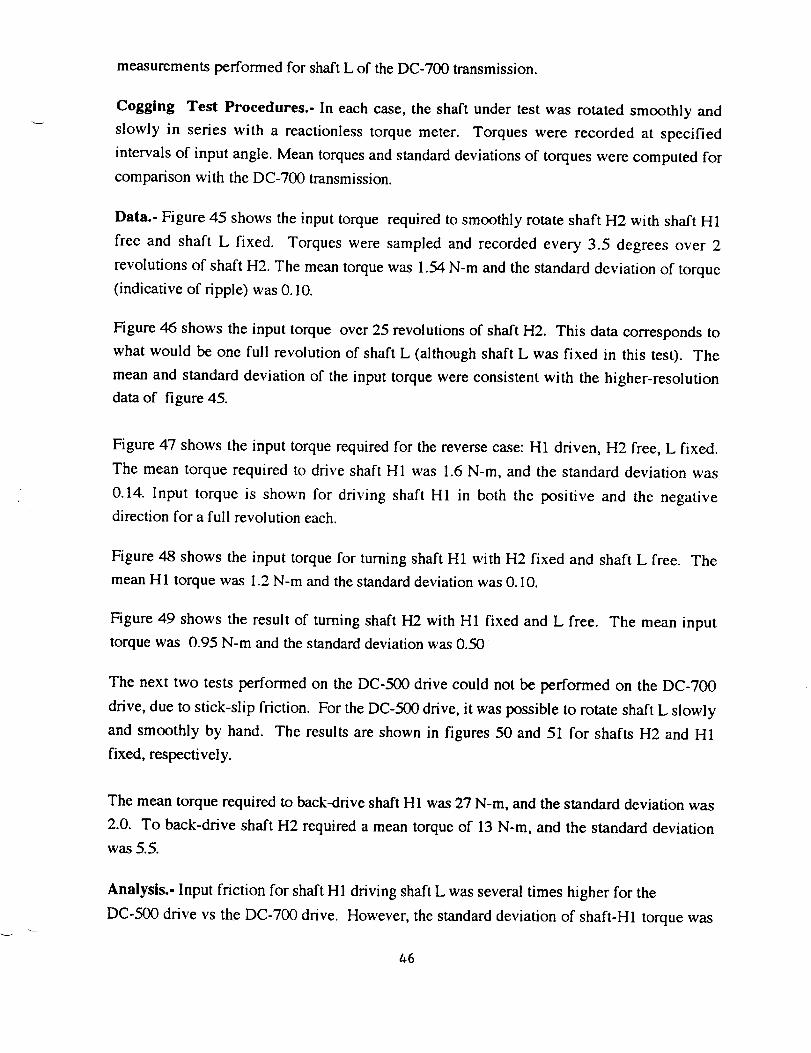
measurementsperformedfor shaftL of theDC-700transmission.
Cogging Test Procedures.- In each case, the shaft under test was rotated smoothly and
slowly in series with a reactionless torque meter. Torques were recorded at specified
intervals of input angle. Mean torques and standard deviations of torques were computed for
comparison with the DC-700 transmission.
Data.- Figure 45 shows the input torque required to smoothly rotate shaft H2 with shaft H1
free and shaft L fixed. Torques were sampled and recorded every 3.5 degrees over 2
revolutions of shaft H2. The mean torque was 1.54 N-m and the standard deviation of torque
(indicative of ripple) was 0.10.
Figure 46 shows the input torque over 25 revolutions of shaft H2. This data corresponds to
what would be one full revolution of shaft L (although shaft L was fixed in this test). The
mean and standard deviation of the input torque were consistent with the higher-resolution
data of figure 45.
Figure 47 shows the input torque required for the reverse case: H1 driven, H2 free, L fixed.
The mean torque required to drive shaft H1 was 1.6 N-m, and the standard deviation was
0.14. Input torque is shown for driving shaft H1 in both the positive and the negative
direction for a full revolution each.
Figure 48 shows the input torque for turning shaft H1 with H2 fixed and shaft L free. The
mean H1 torque was 1.2 N-m and the standard deviation was 0.10.
Figure 49 shows the result of turning shaft H2 with H1 fixed and L free. The mean input
torque was 0.95 N-m and the standard deviation was 0.50 _
The next two tests performed on the DC-500 drive could not be performed on the DC-700
drive, due to stick-slip friction. For the DC-500 drive, it was possible to rotate shaft L slowly
and smoothly by hand. The results are shown in figures 50 and 51 for shafts H2 and H1
fixed, respectively.
The mean torque required to back-drive shaft H 1 was 27 N-m, and the standard deviation was
2.0. To back-drive shaft H2 required a mean torque of 13 N-m, and the standard deviation
was 5.5.
Analysis.- Input friction for shaft H1 driving shaft L was several times higher for the
DC-500 drive vs the DC-700 drive. However, the standard deviation of shaft-H1 torque was
t,6
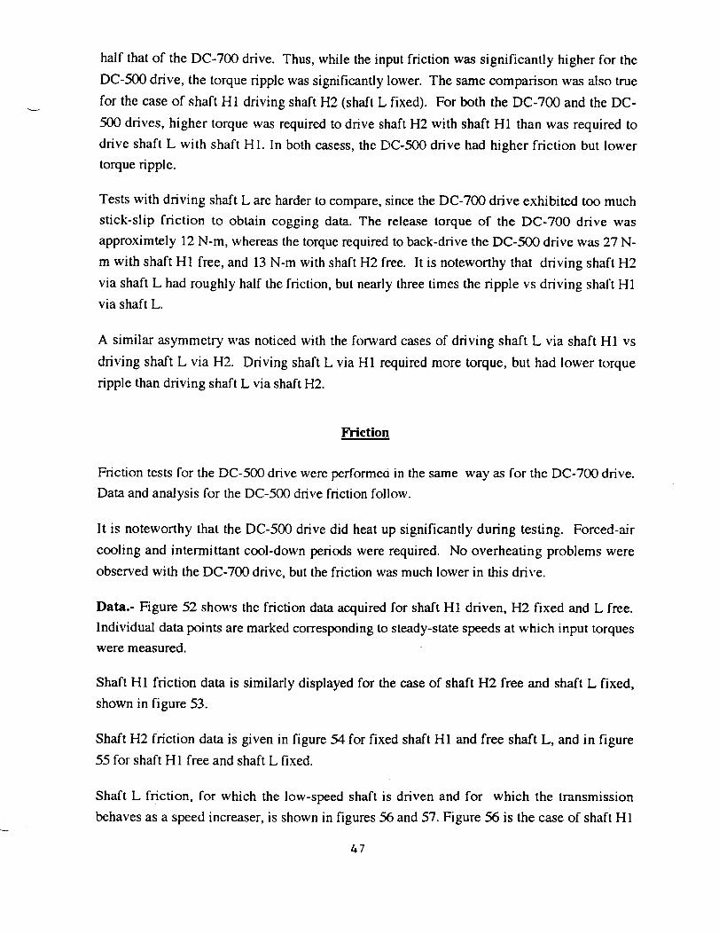
half that of the DC-700 drive. Thus, while the input friction was significantly higher for the
DC-500 drive, the torque ripple was significantly lower. The same comparison was also true
for the case of shaft H 1 driving shaft H2 (shaft L fixed). For both the DC-700 and the DC-
500 drives, higher torque was required to drive shaft H2 with shaft H1 than was required to
drive shaft L with shaft HI. In both casess, the DC-500 drive had higher friction but lower
torque ripple.
Tests with driving shaft L are harder to compare, since the DC-700 drive exhibited too much
stick-slip friction to obtain cogging data. The release torque of the DC-700 drive was
approximtely 12 N-m, whereas the torque required to back-drive the DC-500 drive was 27 N-
m with shaft H1 free, and 13 N-m with shaft H2 free. It is noteworthy that driving shaft H2
via shaft L had roughly half the friction, but nearly three times the ripple vs driving shaft H1
via shaft L.
A similar asymmetry was noticed with the forward cases of driving shaft L via shaft H1 vs
driving shaft L via H2. Driving shaft L via H1 required more torque, but had lower torque
ripple than driving shaft L via shaft H2.
Friction
Friction tests for the DC-500 drive were performe0 in the same way as for the DC-700 drive.
Data and analysis for the DC-500 drive friction follow.
It is noteworthy that the DC-500 drive did heat up significantly during testing. Forced-air
cooling and intermittant cool-down periods were required. No overheating problems were
observed with the DC-700 drive, but the friction was much lower in this drive.
Data.- Figure 52 shows the friction data acquired for shaft H1 driven, H2 fixed and L free.
Individual data points are marked corresponding to steady-state speeds at which input torques
were measured.
Shaft H1 friction data is similarly displayed for the case of shaft H2 free and shaft L fixed,
shown in figure 53.
Shaft H2 friction data is given in figure 54 for fixed shaft H1 and free shaft L, and in figure
55 for shaft H1 free and shaft L fixed.
Shaft L friction, for which the low-speed shaft is driven and for which the transmission
behaves as a speed increaser, is shown in figures 56 and 57. Figure 56 is the case of shaft H1
/,7

free and shaft H2 fixed, and figure 57 is the case of shaft H1 fixed and shaft H2 free.
Analysis.- Like the DC-700 drive, the friction plots for the DC-500 drive are relatively flat vs
speed. This indicates that frictional losses are dominantly due to Coulomb friction. The
friction plots are also consistent with the computed mean torque at low speeds, as measured
in the cogging tests.
Driving shaft L (unloaded) via shaft H1 required roughly 1.2 N-m, and driving shaft L
(unloaded) via shaft H2 required only about half that torque. Similarly, back-driving shaft
H1 (unloaded) via shaft L required approximately 25 N-m, whereas back-driving shaft H2 via
shaft L required about 12 N-m.
Friction torque for driving shaft H1 via H2 vs driving H2 via H1 was nearly symmetric at
roughly 1.5 N-m.
Note that in the tests presented earlier for the DC-700 drive, back-driving shaft H1 via shaft
L required only about 5 N-m, and back-driving shaft H2 via shaft L required about 10 N-m.
Oddly, with the DC-500 drive, it was easier to back-drive shaft H2 (12 N-m) than it was to
back- drive shaft H1 (25 N-m).
It is noteworthy that the DC-500 drive had considerably more Coulomb friction than the DC-
700 drive. For shaft HI, the DC-700 drive had a 35W loss for driving shaft H1 with shaft L
unloaded at the maximum test speed. The same conditions for the DC-500 drive led to over
170W loss.
In backdriving the DC-500 drive, the power loss due to Coulomb friction at shaft L driving
shaft H1 was approximately 130W at the maximum speed tested. Backdriving shaft H2 at
the maximum speed tested required 55W.
The larger Coulomb friction components of the DC-500 drive influence efficiency, resulting
in lower efficiencies. This is particularly true at lower torques, since the frictional torque is
then a significant fraction of the total torque.
Efficiency
Efficiency Test Procedures.- Efficiency tests were conducted identical to those described
previously for the DC-700 drive.
48

Data. - Figure 58 shows the results for the condition of stationary shaft L.
Figures 59 through 66 show the efficiency results for 7 additional (non-zero) output speeds.
Analysis.- At the higher torque levels, efficiencies were measured at about 85%. Efficiencies
dropped off dramatically at lower torques, since the higher Coulomb friction was then a
higher percentage of the net torque. The datapoint markers and the solid vs dashed lines may
be interpreted in the same manner as presented for the DC-700 transmission.
GROUNDED RING (MOMENTUM BALANCED) DRIVE (DC-400)
The DC-400 transmision has a single high speed shaft, referred to as shaft "H", and dual
counterrotating output shafts, referred to as shaft "LI" (inner output shaft) and shaft "L2"
(outer output shaft). The terms "input" and "output" are used in the conventional sense in
that power is typically introduced to a high speed shaft and transmitted out a low speed shaft.
In such cases the transmission is used as a "speed reducer" which amplifies the torque
produced by a high-speed, low torque electromechanical actuator. It should be recognized,
however, that each of the three shafts can input or output power. Efficiency tests, for
example, were performed with both forward and reverse power flows at both high-speed
(input) and low-speed (output) shafts.
In the DC-400 transmission all three shafts are kinematically linked. If one of the shafts is
locked or constrained, then the other two cannot be moved, i.e.,torque and motion transfcr
paths between any two shafts are not independent of the third shaft. The two output shafts
(L1 and L2) counterrotate at equal and opposite speeds. This is in contrast to the DC-700 and
DC-500 transmissions which allow torque and motion transfer between any two shafts with
the third shaft constrained. As a consequence of its kinematic differences with the DC-700
and DC-500 units, the test procedure for DC-400 was quite different from that of the DC-700
and DC-500 units.
The DC-400 transmission was integrated into the test stand as per drawing DC-800-SK, sheet
2, subject to the coupling modifications noted above. Angular linearity, torque cogging,
Coulomb and viscous friction, and power transfer efficiency are presented in this section.
Shortly after tests were initiated, a failure of the drive occurred. Disassembly of the drive
revealed that it had been assembled with an incorrect locknut on the outer output shaft (part
DC-400-15). The outer diameter of the locknut that was used had not been relieved as on the
49
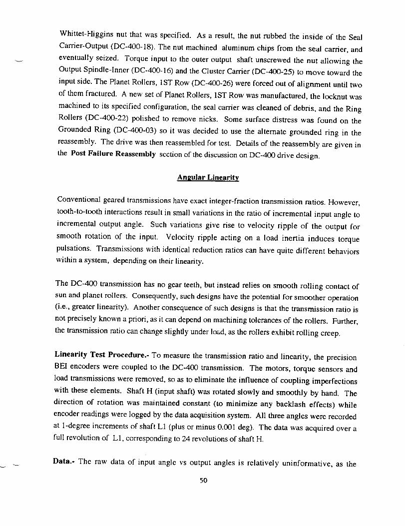
Whittet-Higgins nut that wasspecified. As a result, the nut rubbed the inside of the Seal
Carrier-Output(DC-400-18).The nut machined aluminumchips from the seal carrier, and
eventually seized. Torque input to the outeroutput shaft unscrewedthe nut allowing the
OutputSpindle-Inner(DC-400-16)andtheClusterCarrier(DC-400-25) to move toward the
inputside.The PlanetRollers,1STRow (DC-400-26)wereforcedout of alignment until twoof themfractured. A newsetof PlanetRollers,1STRow wasmanufactured,the locknut was
machinedto its specifiedconfiguration,thesealcarrier wascleanedof debris, and theRing
Rollers (DC-400-22) polished to removenicks. Somesurfacedistresswas found on the
GroundedRing (DC-400-03) so it was decidedto use the alternategrounded ring in the
reassembly.The drive was thenreassembledfor test. Detailsof thereassemblyaregiven in
the Post Failure Reassemblysectionof thediscussiononDC-400drive design.
An_ular Linearity
Conventional geared transmissions have exact integer-fraction transmission ratios. However,
tooth-to-tooth interactions result in small variations in the ratio of incremental input angle to
incremental output angle. Such variations give rise to velocity ripple of the output for
smooth rotation of the input. Velocity ripple acting on a load inertia induces torque
pulsations. Transmissions with identical reduction ratios can have quite different behaviors
within a system, depending on their linearity.
The DC-400 transmission has no gear teeth, but instead relies on smooth rolling contact of
sun and planet rollers. Consequently, such designs have the potential for smoother operation
(i.e., greater linearity). Another consequence of such designs is that the transmission ratio is
not precisely known a priori, as it can depend on machining tolerances of the rollers. Further,
the transmission ratio can change slightly under load, as the rollers exhibit rolling creep.
Linearity Test Procedure.- To measure the transmission ratio and linearity, the precision
BEI encoders were coupled to the DC-400 transmission. The motors, torque sensors and
load transmissions were removed, so as to eliminate the influence of coupling imperfections
with these elements. Shaft H (input shaft) was rotated slowly and smoothly by hand. The
direction of rotation was maintained constant (to minimize any backlash effects) while
encoder readings were logged by the data acquisition system. All three angles were recorded
at 1-degree increments of shaft L1 (plus or minus 0.001 deg). The data was acquired over a
full revolution of L1, corresponding to 24 revolutions of shaft H.
Data.- The raw data of input angle vs output angles is relatively uninformative, as the
50

dataplotsare indistinguishablefrom straightlines To obtain average transmission ratios, the
output angles were fit to equations: H = LI*R1 and H = L2*R2, where the input angle (H)
was fit to the output angles (L1 and L2) via a least-squares fit of the data, yielding
correlations R1 and R2 of the effective transmission ratos.
The resulting transmission ratios were: R1 = 23.98 and R2 = 24.12. Given these average
ratios, gross transmission nonlinearity could be evaluated by comparing the measured angles
L1 and L2 to the ideal angles H/R1 and H/R2 respectively. Figure 67 displays the errors
LI*R1-H and L2*R2-H vs input angle H. The maximum deviation of angle L1 from the ideal
corresponds to approximately 1 degree of input angle, observed at nearly 2000 degrees of
input rotation. The deviation of angle L2 was roughly half as large.
The incremental transmission ratio, R = (delta H)/(delta L), was computed with respect to
both outputs, evaluated at increments of 1 degree of each output. The result is plotted in
Figure 68. The mean incremental transmission ratios were R1=23.97 and R.2=24.11, which
agree closely with the least-squares evaluations of the ratios. The incremental ratio R1 varied
from a minimum of 23.88 to a maximum of 24.05, and had a standard deviation of 0.03. The
incremental ratio R2 varied from a minimum of 24.00 to a maximum of 24.26, with a
standard deviation of 0.03.
Analysis.- The standard deviation of incremental transmission ratio is a reasonable figure of
merit for smoothness. The standard deviation of incremental transmission ratio of the DC-
400, computed at 0.03, indicates that this is a relatively smooth drive, characteristic of
traction-drive designs. By comparison, the DC-700 drive (which incorporates gears) had a
standard deviation of transmission ratio of 0.10, and the DC-500 drive (a traction-drive
design) had a corresponding standard deviation of 0.05. It should be noted that the resolution
limit of the encoders (at 0.001 degree) introduces some error in this computation. Encoder
resolution artifacts can imitate incremental ratio errors approximately as large as the
computed standard deviation of the DC-400 drive. While the computed standard deviation is
comparable to the measurement noise, specific datapoints in the dataset exceed the variations
expected from sensor discretization. Thus, the computed 0.03 standard deviation is believed
to be a realistic measure of the transmission's linearity.
In addition to angular nonlinearity, another source of torque ripple in transmissions is
cogging. Cogging is a quasi-static phenomenon that can be induced by effects such as
51

variable binding due to imperfect tolerances. Cogging can have both reproducible and
stochasticcomponents.For example,a flat spoton a roller would result in a reproducible
torquedisturbance,whereasdustor dirt betweenrollerscould introduce torque variations that
are not repeatable.
Cogging Test Procedure.- Accurate measurement of cogging requires a smooth input driver.
Further, such tests should be performed quasi-statically, to avoid affecting the data with
dynamic terms (e.g., due to angular nonlinearity). For such tests, it is not necessary that the
input driver enforce a steady velocity, provided the accelerations are low. Thus, manual
rotation is a good candidate input driver.
Cogging tests were performed on shafts H (input) and L1 (inner output) of the DC-400, in
each case with the remaining shafts unconstrained. Shaft H was rotated for approximately
500 degrees in both the positive and negative directions. The rotation was induced by hand,
in series with the input torque meter. During this rotation, the input torques were datalogged
vs shaft angle.
Shaft L1 was more difficult to drive, since the friction was too high to rotate it manually.
The NAS-300A load transmission was used, in this case, to amplify manually-induced drive
torques. The input shaft of the NAS-300A was manually rotated, and the output of the NAS-
300A drove shaft L1 (inner output shaft) of the DC-400 transmission through a reactionless
torque meter. Since the NAS-300A is a relatively smooth transmission, this approach
enabled slow, smooth excitation of shaft L1. Further, since the torque transducer was located
between the NAS-300A output shaft and shaft L1 of the DC-400, the torque measurements
did not include any imperfections of the NAS-300A. The manual rotation produced a shaft
L1 rotation of plus and minus 245 degrees. Torques acting on shaft L1 were datalogged vs
the angle of shaft L1.
Cogging of shaft L2 could not be measured directly. The hollow harmonic drive (load
transmission) on shaft L2 did not permit a smooth enough excitation to obtain valid cogging
data. The cogging of shaft L2 may be expected to be similar to that of L1.
Data.- Figure 69 shows the results of the positive and negative rotations of shaft H. The
mean torque (plus and minus) is 1.56 N-m and the standard deviation is 0.12 N-m. There are
three noticeable torque increase "humps" in the data. Windowing a section of data which
excludes these relatively large, low-frequency variations results in reducing the standard
deviation by half (to 0.06 N-m).
52

Figure70 showstheresultsfor shaftL1. Themeantorque(plus andminus) is 36.8 N-m and
thestandarddeviation is 4.8 N-m. Again, windowing a sectionof datawhich excludesthe
severalrelatively large,low-frequencyspikes,theresultingstandarddeviation is significantlylessat 2.6N-m.
Analysis.- The data shows that torque nonlinearity is dominated by Coulomb friction. The
Coulomb friction was 1.56 N-m for shaft H and 36.8 N-m for shaft L1. The cogging data
showed occasional significant variations in input torque (on the order of 30%). Such
variations may be due to small eccentricities of the rollers. The higher-frequency torque
variations were much smaller -approximately 0.1 and 3.0 N-m RMS for shafts H and L1,
respectively.
The ratio between input Coulomb friction and the Coulomb friction of shaft L1 is 23.6, which
is remarkably close to the reduction ratio. This observation suggests that the friction load
may be coming from a common source. In that case, one would expect to find the Coulomb
friction losses distributed among the 3 shafts, rather than find additive losses for each shaft
independently.
The input friction and cogging for shaft H of the DC-400 were very close to those measured
on the DC-500 (dual-input) transmission inputs (with shaft L locked). The inner output
friction (shaft L1) of the DC-400 was also roughly comparable to shaft-L (output) friction of
the DC-500 with shaft H2 fixed. The DC-700 transmission (which incorporated gear teeth)
had lower friction but greater torque ripple.
Frietlon.
The cogging tests revealed the presence of strong Coulomb friction. Accounting for such
friction is an important element of reconciling transmission efficiencies. Ordinarily, a
transmission exhibits a speed-dependent friction term in addition quasi-static friction. Tests,
data and analysis of speed-dependent friction of the DC-400 transmission are presented
below.
Friction Test Proeedure.-Friction tests were performed by driving each shaft, one at a time,
with the remaining two shafts unconstrained. The driving torque was measured for each case
at selected drive speeds, both positive and negative. At each speed, approximately 5,000
samples of the drive torque meter were acquired over 5 seconds, sampled at lkHz. The
53
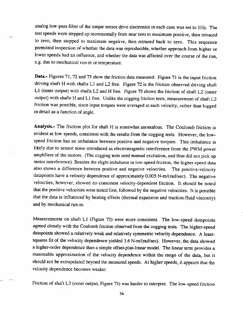
analoglow-passfilter of thetorquesensordriveelectronicsin eachcasewassetto 1Hz. The
testspeedswere steppedup incrementallyfrom nearzeroto maximumpositive, then retraced
to zero, then stepped to maximum negative, then retracedback to zero. This sequencepermittedinspectionof whetherthedatawasreproducible,whetherapproachfrom higheror
lower speedshadan influence,andwhetherthedatawasaffectedover the courseof therun,
e.g.dueto mechanicalrun-in or temperature.
Data.- Figures71, 72and73 showthefriction datameasured.Figure 71 is the input friction
driving shaft H with shaftsL1 andL2 free. Figure72 is thefriction observeddriving shaft
L1 (inner output) with shaftsL2 andH free. Figure73 shows the friction of shaft L2 (outer
output) with shafts H and L1 free. Unlike the cogging friction tests, measurement of shaft L2
friction was possible, since input torques were averaged at each velocity, rather than logged
in detail as a function of angle.
Analysis.- The friction plot for shaft H is somewhat anomalous. The Coulomb friction is
evident at low speeds, consistent with the results from the cogging tests. However, the low-
speed friction has an imbalance between positive and negative torques. This imbalance is
likely due to sensor noise introduced as electromagnetic interference from the PWM power
amplifiers of the motors. (The cogging tests used manual excitation, and thus did not pick up
motor interference). Besides the slight imbalance in low-speed friction, the higher-speed data
also shows a difference between positive and negative velocities. The positive-velocity
datapoints have a velocity dependence of approximately 0.005 N-m/(rad/sec). The negative
velocities, however, showed no consistent velocity-dependent friction. It should be noted
that the positive velocities were tested first, followed by the negative velocities. It is possible
that the data is influenced by heating effects (thermal expansion and traction-fluid viscosity)
and by mechanical run-in.
Measurements on shaft L1 (Figure 72) were more consistent. The low-speed datapoints
agreed closely with the Coulomb friction observed from the cogging tests. The higher-speed
datapoints showed a relatively weak and relatively symmetric velocity dependence. A least-
squares fit of the velocity dependence yielded 1.6 N-m/(rad/sec). However, the data showed
a higher-order dependence than a simple offset-plus-linear model. The linear term provides a
reasonable approximation of the velocity dependence within the range of the data, but it
should not be extrapolated beyond the measured speeds. At higher speeds, it appears that the
velocity dependence becomes weaker.
Friction of shaft L2 (outer output, Figure 73) was harder to interpret. The low-speed friction
5t_

wasapproximately45 N-m, significantlyhigherthanthe36.8N-m Coulomb friction of shaft
L1. Although the torque meter for shaft L2 is not well sized to accurately measuresuchrelatively low torques,thedifferencebetweentheL2 andL1 Coulombfriction torques(8 N-
m) is 0.7% of the L2 torque meter's range, which lies within the claimed 0.1% linearity.
Thus, the measurements should be reliable in the result that shaft L2 Coulomb friction is
approximately 20% higher than that of shaft L1.
There does appear to be a relatively weak dependence of the L2 friction on velocity.
However, the data cannot support a reliable conclusion regarding the sensitivity. It is also
noteworthy that the positive velocities showed a stronger velocity-dependent friction than the
negative velocities. As with the input friction data, however, this may be due to slow thermal
or mechanical wear variations during the data collection.
The relatively large Coulomb friction and relatively weak velocity-dependent friction
behavior observed is consistent with traction-drive designs.
Efficiency
Efficiency tests were performed on the DC-400 transmission under nearly 200 steady-state
conditions of speed, input torque, and ratio of output torques. The data included power flow
in both the "forward"condition (power into high-speed shaft, power out of low-speed shafts)
and "reverse" (power into shafts L1 and L2, power out of shaft H).
Various constraints of the test equipment and of the DC-400 transmission limited the
conditions to relatively low speeds and torques (roughly half the rated limits). The
harmonic-drive load transmission limited the velocity of the tests to input speeds between
-105 rad/sec and 105 rad/sec. Since the wave generator and flex spline of the harmonic drive
were not adequately restrained in the axial direction, this transmission would bind up at
higher speeds and under some conditions of direction of rotation and direction of power flow.
In addition, axial drift of the harmonic-drive flex spline led to excessive friction under some
test conditions of higher speeds and torques, corrupting the efficiency data. It was
anticipated that the efficiency tests would be limited by the power limitations of the
Compumotors used. The Compumotors were limited in both speed and torque to
approximately half of the DC-400 rating. However, it was found that the Compumotors'
speed limits were higher than the harmonic-drive speed constraint, so the Compumotors did
not present a binding constraint on speed. In addition, although the Compumotors were not
capable of exerting the full rated input torque of the DC-400, it was found experimentally
55

that the DC-400 could not acceptinput torquesin excessof 17N-m (150 in-lbf), so the
Compumotortorquelimits werealsonot bindingconstraints.
The Uniq motor presentedanotherconstrainton theefficiency tests. This motor performed
well asa power source,but it wasnot well behavedasa powersink. Somedatawas taken
with this motor actingasa powersink, but the loadtorqueprovidedwas lesswell regulated.
This constraintlimited the measurementsof forwardefficiency (power in at shaft H andoutat shaftsL1 andL2).
The DC-400 designpresentedadditionalunexpectedconstraintson the torqueswhich could
be tested.Due to internalpreloadinglimits at thegroundedring, it is most desirableto keepthe two low speedshaft torques(L1 and L2 torques)within approximately 30% of eachother to avoid the dangerof slip at the groundedring. A more surprising limit was themaximuminput torquethat thetransmissioncouldaccept.Although it was ratedfor 36 N-m
(320 in-lbf) input torque, it was found that the transmission misbehaved (appeared to induce
roller slip) at input torques in excess of 17N-m (150 in-lbf).
The DC-400 was thus tested to the limits of the torques it could support, but the tests spanned
only about 35% of the rated speed.
Efficiency Test Procedure.- For each condition of speeds and torques, the transmission was
driven as follows. Shaft H (input) speed was regulated by driving the input Compumotor in
synchronous mode. Shaft L1 torque was regulated by driving the second Compumotor (via
the NAS-300A transmission) in torque mode. The Uniq motor was driven by a soft velocity-
control loop. As the Uniq motor velocity control command was varied about the enforced L2
velocity, the resulting torque exerted by the Uniq motor (via the harmonic-drive load
transmission) on L2 varied. Correspondingly, the torque on shaft H varied (by approximately
1/24 of the L2 torque change). Under such control, various combinations of shaft speeds and
torques could be produced.
Data was acquired at steady-state input velocities of -105, -70, -35, 35, 70 and 105 rad/sec.
At each speed, tests were performed at steady-state input torques ranging between
approximately plus and minus 17N-m (150 in-lbf). At each combination of speed and input
torque, torque conditions on shafts L1 and L2 were tested, typically for 5 conditions of output
torque ratio ranging from approximately 0.7 to 1.4.
Data.- Figure 74 displays a summary of data for the transmission efficiency in "reverse"
56

operation(power input to L1 andL2, poweroutput from H). Eachof the curvesdisplayed
comprisesa set of data taken at constantinput velocity. The 6 curves represent input
velocitiesof -105, -70, -35,35, 70 and 105rad/sec.For eachcurve, specific datapointsarenoted, totaling 39 conditions. For eachcondition, the two output shafts(I_,1and L2) were
driven with approximatelyequal torquesandspeeds(and thusapproximatelyequalpower).
The Compumotor on shaft H was usedas a power sink. The power extracted at port Hdivided by thepowerinput to shaftsL1 andL2 is plottedastheefficiency.
Figure 75 displayscorrespondingdata for conditionsof "forward" power transfer(powerinto shaft H andout of shaftsL1 andL2).
Figure 76 offers a different visualizationof the data. Efficiencies are plotted vs shaft H
torque, rather than vs input power. Lines on this plot are, again, groups of datapointsacquired at constantspeed. All 12 lines from Figs 74 and 75 (both forward and reverse
power flow data)are includedon this commonplot. From this figure, it is evident that theefficiency improves with higher input torques. This observation is consistent with a
hypothesisthat transmissionlossesareprimarily attributableto Coulomb-typefriction, likely
due to roller preloading. Such friction seemsto be independentof speedand of output
torque. To furtherexplorethis hypothesis,thepowerlossfor eachcondition wascomputed,and theequivalent friction torquewhich couldaccountfor this loss (with respectto shaft H)
was computed. A display of the equivalent loss torques (computed from the reverseefficiency data)is givenin Figure77.
Additional tests were performed with imbalanced torques L1 and L2. At input speeds of plus
and minus 35, 70 and 105 rad/sec, and at input torques of plus and minus 80 in-lbf, 110 in-lbf
and 150 in-lbf, the torque ratio between output shafts L1 and L2 was varied.
Efficiency data is plotted for each input speed, displaying efficiency vs output torque ratio,
for lines of constant input torque. Nine such plots are included. Figures 78 through 83 show
the _reverse" efficiencies (power sources at L1 and L2, power sink at H) for input speeds of
-105, -70, -35, +35, +70, and +105 rad/sec, respectively. Figures 84, 85 and 86 show similar
tests for "forward" efficiency (power sourced to shaft H, power sinks at L1 and I_,2). These
plots display the results for input speeds of +35, +70 and +105 rad/sec, respectively.
Due to axial drift of the harmonic-drive wave generator, tests could not be performed for
forward power flow with a negative input velocity. In addition, the data for forward power
flow at +105 rad/sec was limited to conditions of L1 torque less than L2 torque. Increasing
57

torqueonL1 higher thanthetorqueonL2 resultedin rollerslip.
Analysis.- Figure 75, which displays the "forward" efficiency values, indicates efficiencies as
high as 92%. (Even higher efficiencies were measured when the output shaft torques were
not balanced, favoring power flow via shaft L2). Figure 75 indicates that it is typically true
that higher power transfers result in greater efficiency. The curve corresponding to an input
velocity of +35 rad/sec seems to be an exception to this trend. Note, though, that the
anomalous points occur at relatively low torques and at the lowest speed, making the
measurement sensitivity poorer and the susceptibility to noise (such as the EMI produced by
the motor amps and picked up by the torque-sensor electronics) higher.
The trend to higher efficiencies at higher powers is indicative of an equivalent "fixed cost" of
transmission losses, which is proportionately less important as input powers increase. To
test such a model of efficiency, Fig 76 was genet'ated, in which all 12 of the constant-speed
data sets are plotted (both positive and negative input velocities, and positive and negative
power flows) vs input torque, rather than vs input power. For the most part, the lines of Fig
76 converge. This suggests that the efficiency is primarily a function of input torque. As the
input torque increases, the efficiency increases. This is consistent with having a fixed input
friction, which represents a smaller percentage loss as the input torque increases.
Figure 77 shows the computed equivalent input-shaft friction which could account for the net
power loss for each reverse-efficiency measurement. If the losses could be explained by pure
Coulomb friction, then the loci of Fig 77 would appear as coincident, horizontal lines. The
computed Coulomb friction, however, varies from less than 1 N-m to nearly 6 N-m. It is
possible that the higher computed friction values reflect additional friction introduced by the
harmonic-drive flex spline. The lower computed friction values are more nearly flat vs input
power, and thesetorque values are closer to the measured input-shaft friction with unloaded
output shafts. Overall, this plot suggests that the DC-400 efficiency at different speeds and
torques can be reasonably estimated by considering losses due to Coulomb friction,
essentially independent of load. In addition, this plot suggests that harmonic-drive friction
did influence the measurements, and it suggests a range for this influence.
In both Figures 74 and 75, the data at positive input speeds indicates a higher efficiency than
the corresponding data at negative input speeds. There is no obvious reason why the DC-400
transmission data should have a preferred direction of rotation, and no such asymmetry was
observed in the friction. This phenomenon is likely attributable to the test-stand problem
with the harmonic-drive components. The direction of axial drift of the harmonic-drive flex
58

spline was a function of the direction of rotation. When this component translated into
contact with its confining thrust washers, the resulting friction would affect the
measurements, yielding a lower apparent efficiency. It could not be observed when such
internal friction arose. However, this flaw in the test rig could only decrease the apparent
efficiency. Thus, the highest measured efficiencies are the most credible.
The highest measured efficiencies exceeded 95%. As expected, based on the measured
Coulomb friction, the highest efficiencies typically occurred at the highest torque loading.
Some exceptions are notable. For example, Fig 83 (reverse efficiency at input speed +105
rad/sec) shows an efficiency at 150 in-lbf input torque which is lower than that of the 80 and
110 in-lbf input torques. This condition likely indicates the onset of roller slip in the DC-
400 at this condition of speed and torque.
The differential output torque measurements (Figs 78 through 86) gave a surprising result.
Efficiencies were typically higher when shaft L2 (outer output) was driven harder than shaft
'L1 (inner output). The friction measurements indicated that shaft L2 had a higher friction
than shaft L1 (when the remaining two shafts were free). Thus, it would seem that
efficiencies should be higher when more power is transmitted through shaft L1 than through
shaft L2. As the output torque ratio LI/L2 varied from about 0.7 to about 1.4, the efficiency
fell by (typically) several percentage points.It may be that this variation is an artifact of the
test-stand flaws (particularly the harmonic drive friction), or it may be that the effect is a
result of the complex kinematic interactions among the differential rollers of the DC-400
drive.
Finally, the efficiency data also provides information regarding roller creep vs load. The data
from Fig 74 was used to compute the speed ratio from input shaft H to output shaft L1
(output shaft L2 angle could not be measured directly under load). The ratio of input to
output speed was seen to change as the torque on L1 increased. For the data of Fig 8, shaft
L1 was driven with a power source. As a result, this shaft ran somewhat faster than predicted
by the transmission ratio (as measured under unloaded conditions). Alternatively, the speed
ratio from H to L1 decreased as the torque on shaft L1 increased. The result is shown in Fig
87. Creep between shafts H and L1 apparently changes linearly as a function of applied
torque. The lone out-lying datapoint (at ratio=23.07) corresponds to an input torque in
excess of 150 in-lbf. Thus, this datapoint likely includes some roller slipping.
59

DISCUSSION OF RESULTS
Several comparisons can be made between the performance of the Differential Roller-Gear
Drive (DC-700) and the Differential Roller Drive (DC-500). As expected, the linearity of the
Roller Drive is superior to that of the Roller-Gear Drive because the transfer of motion
through rollers is smoother than through gears. The standard deviation of non-linearity in the
Differential Roller Drive was approximately half that in the Differential Roller-Gear Drive.
Variations in linearity result in small variations in the ratio of incremental input angle to
incremental output angle which give rise to velocity ripple of the output. Velocity ripple
acting on a load inertia induces torque pulsations. In a similar vein, cogging or torque ripple
tests showed that the Differential Roller Drive is smoother as a speed reducer than is the
Differential Roller-Gear Drive. Additionally the Differential Roller-Gear Drive exhibited
some stick-slip in a back driving mode. Attempts to conduct cogging tests driving the output
or low speed shaft with both input shafts free were unsuccessful because of a significant
breakaway torque. The Differential Roller Drive was smoother in a back driving mode. In
any robotic application where variations of output velocity and torque are critical to
performance acceptability, use of a roller drive would be advantageous.
For simplicity of design a varible preload system was not incorporated into the Differential
Roller Drive. It is preloaded at assembly with shims. At first assembly the preload was set at
100% of rated torque. The resulting tare torque was quite high, so the preload was reset at
approximately 80% with the view that, after run-in, the drive would relax allowing an
increase of preload to full rating while still maintaining a reasonable level of tare torque.
Tests were therefore limited to 80% of full torque rating to avoid risking roller slip.
Although simpler mechanically, the Coulomb friction losses in a fully preloaded drive are
almost constant regardless of the torque (or power) being transmitted so that efficiency losses
are incurred whenever levels of torque transfer are less than full rating. Friction losses at
zero power output were five times as great in the Roller Drive as in the Roller-Gear Drive
when each drive was operated as a speed reducer. Details of friction losses through the
various torque transfer paths at zero power output are shown in Table XI.
Differential Roller-Gear Drive efficiencies at the highest output speed at which
measurements were taken (4.9 rad/sec) ranged from 87 to 94% at full rated torque, and 86 to
94.5% at 20 percent of full rated torque. (In a differential drive the efficiency (power
out/power in) at a set value of output speed and torque depends on the combination of input
speeds used to obtain the desired output speed). In contrast, Differential Roller Drive
efficiencies were 75 to 83% at 80 percent of full rated torque, and 52 to 83% at 20 percent of
60

full ratedtorque. In assessingtheperformanceof theDifferential Roller Drive it appearsthat
the higher friction lossesand lower part loadefficienciesincurred by useof a full preloadsystemmake the incorporation of a variablepreloadsystemmandatory in future designs.
The efficiencies measuredarestrictly thoseassociatedwith frictional losses. Lossesinefficiency in differential drives canalso result from recirculatingpower. When toll1 and
toll2 are of the same sense, then the output speed will be less than the greater input speed
divided by R. One of the two input torques will be negative (that input will be a power
absorber or brake rather than a driver). There will then be a recirculating power loss. This
will generally be the operating mode of the differential drive. It will be used with two
unidirectional variable speed inputs to produce low magnitude bidirectional output speeds,
with a non-rotating output achievable without having to stop either input. This eliminates the
stick-slip uncertainties associated with starts and stops. Table XII shows the combinations of
input and output angular velocities at which frictional efficiencies (defined as the ratio of
power out to power in) were measured. Some of those combinations of angular velocity
result in recirculating power losses. In those cases the system efficiency will be the product
of frictional efficiency and differential efficiency.
One of the ideosyncracies of motion and torque transfer through preloaded rollers revealed
itself in measurements of ratios between each high speed or input shaft and the low speed or
output shaft (with the second high speed shaft fixed), and from one high speed shaft to the
other high speed shaft (with the low speed shaft fixed) in the Differential Roller Drive. The
nominal design ratio from either high speed shaft to the low speed shaft is 24:1. The ratio
from shaft H1 (inner input shaft) to output shaft L was measured as 23.5:1 with zero torque
restraint on output shaft L. The ratio from shaft H2 (the outer input shaft) to output shaft L
was measured as 24.08:1 with zero torque restraint on output shaft L. These ratios differ by
2.5%. In preloaded rollers a loss in motion known as roller creep occurs in the contact
between each roller pair. The torque transfer path from shaft H1 to shaft L goes through one
set of sun-first planet, one set of first planet-second planet, and one set of second planet-ring
contacts (in the rotating ring roller cluster) to shaft L. The torque transfer path from shaft
H2 to shaft L goes through one set of sun-first planet, one set of first planet-second planet,
and one set of second planet-ring contacts (in the stationary ring roller cluster), and thence
through the second planet-ring contacts in the rotating ring cluster to shaft L. Creep in the
additional set of roller contacts accounts for the 2.5% difference in ratios. The small
difference in ratios means that identical counterrotating speeds of shafts H1 and H2 will not
result in a stationary shaft L. The speeds of shafts H1 and H2 must differ by 2.5% to produce
a stationary shaft L.
61

Kinematicbehaviorof theMomentumBalanced(GroundedRing)Drive wasvery promising.It was the smoothestof thethreedrive testedexhibiting a standarddeviation of incremental
transmissionratio of only 0.03.Reductionratiosfrom theinput to thecounterrotatingoutputs(designvalue = 24) were 23.98and24.12at zeroload, andchangedabout 2% due to roller
creep at the maximum load.. Cogging torques were low, and friction losses were
predominantly due to Coulomb friction. Constraintsof the test equipment limited test
conditionsto relatively low speeds,andanoverestimateof the initial preloadsettingcauseda
roller slip at half theratedcapacity,but testresultswereverypromisingwithin theboundsof
the test conditions. As with the Differential Roller Drive, the penalties incurred by fixedpreloadwereapparent.Efficienciesat low torqueswerelow,andthe uncertaintiesassociated
with setting the initial preload level led to roller slip. The 95% efficiency obtained atmaximum torque is quite satisfactory, however.A modification of the procedureused forsettinginitial preloadlevel is indicated.
\
The Momentum Balanced(GroundedRing) Drive exhibiteddifferencesin efficiency with
positiveandnegativeinputrotationsalthoughthereis noasymmetryinthedrive.The negativerotation direction resultedin lower efficienciesdueto problemswith extraneousfriction in
theL2 shaftcausedby a thrustreactioonin theharmonicdrive elements.Thereforeonly theefficiency dataobtainedfrom thepositiverotationtestsareconsideredvalid.
62

SUMMARY OF RESULTS
1. Two differential (dual input, single output) drives (or transmissions), cach rated at 295
rad/sec (2800 rpm) input speed, 450 N-m (4,000 in-lbf) output torque, and 5.6 kW (7.5hp)
were designed, fabricated, and tested. The Dual Input Differential Rollcr-Gear Drive (DC-
700) has a planetary roller-gear system with a reduction ratio (one input driving the output
with the second input fixed) of 29.23: 1. The Dual Input Differential Roller Drive (DC-500)
has a planetary roller system with a reduction ratio of approximately 24: 1. Each of the
differential drives features dual roller-gear or roller arrangements consisting of a sun, four
first row planets, four second row planets, and a ring. Both drives are lubricated with a
charge (non-recirculating) of commercial traction fluid. Test results reported for the two
differential drives include angular and torque ripple (linearity and cogging), viscous and
Coulomb friction, and fo_vard and reverse power efficiency.
2. A momentum balanced drive ( single input with two counterrotating, equal speed outputs )
was also designed, fabricated and tested. The Momentum Balanced (Grounded Ring) Drive
(DC-400) features a unique "grounded ring" design which makes possible a reduction in size
and weight of approximately 40% when compared to a conventional design. The drive is
rated at 302 rad/sec (2880rpm) input speed, dual output torques of 434Nm(3840 in-lbf) and
10.9kw (14.62hp). The drive features a planetary roller system with five first and second row
planets and a reduction ratio from the input to the dual counterrotating outputs of 24: 1.
3. Standard deviation in linearity of the Differential Roller-Gear Drive was 0.1, and that of
the Differential Roller Drive was 0.05. As expected motion and torque transfer through
rollers is smoother than through gears.
4. Cogging tests to measure torque variations were conducted by smoothly rotating one input
by hand with the second input locked and zero torque applied to the output. The Differential
Roller-Gear Drive had a mean torque of .26N-m (2.3 in-lbf) due to Coulomb friction with a
standard deviation (torque ripple) of .12N-m (1.06 in-lbf) indicating cogging. The
Differential Roller Drive had an average mean torque of 1.5N-m (13.3 in-lbf) due to
Coulomb friction with an average standard deviation (torque ripple) of. 11N-m (.97 in-lbf).
5. Frictional power loss was measured in both differential drives for all torque transfer paths
through the drives. At 140 rad/sec input speed to one input with the second input locked and
the output free, power losses were 35 W (.047 hp) in the Differential Roller-Gear Drive and
170 W (.227 hp) in the Differential Roller Drive.These values are, respectively, .63 and 3
63

percentof full rating. The relativelyhigh valuesof coggingtorqueand zero power frictionloss in the Differential Roller Drive aredue to the useof a full roller preload systemrather
thana cam-acting variable preioad system.This resultsin frictional lossesat zero power
outputwhich approximatethoseatfull ratedpoweroutput.
6. Efficiency (defined as the ratio of power out to power in) was measured for both
differential drives at four output speeds,four combinationsof dual input speedsfor each
output speed,and four torque levels. For the Differential Roller-Gear Drive efficienciesrangedfrom 75% at nearzero power throughput to 95% at the maximum power level. For
the Differential Roller Drive efficiencies ranged from less than 10% at near zero power
throughput to 86% at the maximum power level. The highest measured efficiencies were
obtained with the drives operating as conventional speed reducers. The low efficiencies of
the Differential Roller Drive at low power throughputs are the result of full preloading.
7. The momentum balanced drive performed as expected kinematically.The measured
reduction ratios between the input and the counterrotating outputs were 23.98:1 and 24.12:1
at zero load. A change in ratio of 2% due to roller creep was noted as output torque was
increased to 250Nm (2200 in-lbf) The standard deviation of incremental transmission ratio
was 0.03. It was the smoothest of the threee drives tested. Because of kinematic constraints,
cogging test were conducted by rotating one of the shafts manually with the other two shafts
free. The input shaft mean cogging torque was 1.56Nm (13.8 in-lbf). The inner output shaft
mean cogging torque was 36.8Nm (325.6 in-lbf) with a standard deviation of 4.8Nm (42.8 in-
lbf). Nonlinearity was dominated by Coulomb friction, as expected. In friction tests, when
torque was inputted to the high speed input shaft, there was only a small speed dependence.
8. The momentum balanced drive successfully equilibrated torques among its three shafts. A
given input shaft torque could be balanced by a range of output shaft torques. While the ratio
of output torques was varied from 0.55 to 1.8, the sum of the output torques remained nearly
constant for a given input torque.
9. Efficiencies of the momentum balanced drive were determined in both the forward mode
(speed reducer) and reverse mode (speed increaser). Data were taken at three input velocities
(both positive and negative) with equal torques on the output shafts, and then with output
shaft torque ratios, TL1/TL2, ranging from 0.55 to 1.8. Efficiency improved with increasing
torque and generally decreased with increasing speed. At maximum torque effficiency
approached 95%. The effect of output torque ratio TL1/TL2 was inconsistent. When operated
in the reverse mode, efficiencies decreased slightly with increasing torque ratio; when in the
64
forwardmode, torqueratic_hadlittle effectonefficiency.
10. Limitations in thetest standmadeit impossibleto test themomentumbalanceddrive up
to its full ratedspeed.The harmonicdrive componentsdevelopedthrust loads which were
unexpected.A major redesignof theteststandwouldhavebeenrequired to accomodatethe
thrust loads.This wasnot possible,but thrustwasherswereaddedto makepossible testingovera reasonablespeedrange.
11. The disadvantages of fixed preload again became apparent in these tests . Part load
efficiencies were low, and the level of initial preload was evidently set too low. The latter
resulted in roller slip at approximately 50% of the drive rating.
65

REFERENCES
1. Steinetz, Bruce M., Rohn, Douglas A., and Anderson, William J.: Evaluation of a
High Torque Backlash-Free Roller Actuator. Presented at the 20th Aerospace Mechanisms
Symposium, May 7-9, 1986. NASA CP2423, pp. 215-240.
2. Anderson, William J.: Dual Counterrotating Output Torque and Speed Matched
Drives. Final Report for NASA Lewis Research Center, Contract NAS 3-25576, June, 1989.
3. Anderson, William J.: Traction Drives for Reaction Free and Momentum Balanced
Systems, and Zero Stick-Slip Robotic Drives. Final Report for NASA Lewis Research
Center, Contract NAS 3-26570, August, 1992.
4. Anderson, William J., and Shipitalo, William: Roller-Gear Drives for Robotic
Manipulators. Final Report for NASA Lewis Research Center, Contract NAS 3-25282,
August 1988.
5. Anderson, William J., and Shipitalo, William: Roller-Gear Drives for Robotic
Manipulators: Design, Fabrication and Test. Final Report for NASA Lewis Resarch Center,
Contract NAS 3-25803, September, 1991.
6. Buckingham, E.: "Manual of Gear Design". The Industrial Press, New York.
7. Roark, Raymond J., and Young, Warren C.: Formulas for Stress and Strain. McGraw-
Hill, Inc., 1982.
66

I,-4
67

68

I-II-I
6g

TABLE IV
DC 700 GEAR MEASUREMENTS OVER PINS
GEAR
SUN "a" (input side)
SUN"a"(outputside)
lst. PLANET, ylNOS. I&2
NOS. 3&4
NOS. S&6
NOS. 7&8
NOS. 9&IO
NOS. 11&12
NOS. 13&14
NOS. 15&16
i 1st. PLANET, x 1IIWlTH l&2 yl
PRINT DIM.in.
.9768/.9757
MEASURED
0.9772
DIFFERENCEFROM
HIGH
0.0004+
.9768/.9757 0.9772 0.0004+
.8423/.8414.8424/.8423 0.OO01+/0
.8425/8423 0.0002+/0
.8421/.8424 0.0002-/0.OO01+
.8425/.8426 0.0002+/0.0003+
.8424/.8425 0.0001+/0.0002+
.8422/.8425 0.0001-/0.0002+
.8419/.8420
.8418/.8419
0.0004-/0.0003-
0.0005-/0.0004-
INDEX
ERROR, in.
1.9961/1.9947
1.9954/1.9954 0.0007-/0.0007- 0.0008 2
IWITH 3&4 yl 1.9953/1.99541.9934/1.9934
0.0008-/0.0007- 0.0002 Z
0.0007-/0.0007- 0.0008 1
0.001-/0.0007-WITH S&6 ylWITH 7&8 yl
WITH 9&10 ylWITH 11&12 yl
WITH 13&14 yl
WITH 15&16 yl
2nd. PLANET, x2NOS. I&2
3.6975/3.6963
O.OOO1
0.0012-/0.O01- 0.0003 1
0.0021-/0.O016- 0.0018 1
1.9931/1.9954
1.9949/1.9951
1.9940/1.9945
0.0003-/0.0003- 0.00041.9958/1.9958
1.9946/1.9950 0.O005-/0.OOll- 0.0006 1
3.6968/3.6968
NOS. 3&4 3.6965/3.6964
3.6964/3.6964
3.6968/3.6968
O.0007-/0.0007- 1
0.001-/0.O009- 2
0.0Oll-/O.0Oll- 2
0.0009-/0.001-3.6966/3.6965
3.6965/3.6965 0.001-/0.001- 2
3.6965/3.6965 0.O01-/O.001- 2
1
3.6968/3.6968
0.0007-/0.0007-
0.0007-/0.0007-
9.2989 0.0021- 1
9.2987* 0.0023- 2
NOS. S&6
NOS. 7&8
NOS. 9&IONOS. 11&12
NOS13&14
NOS. 15&16
RING, c 9.2981/9.3010NO.1
NO.2
*Average ofsixreadings
CLUSTER NO
7O

TABLE V
DC 700 ROLLER MEASUREMENTS
ROLLER
SUN "a" (input side)
SUN "a" (output side
1st. PLANET, y 1
PRINT DIM.,in.
.8655/.8653
.8655/.8653
.7223/.7221
MEASURED
.8655/.8655
.8655/.8655
NOS. I&2 .7222/.7223
NOS. 3&4 .7223/.7222
NOS. S&6 .7222/.7222
NOS. 7&8
1.9157/1.915S
NOS. 9&10
NOS. 11&12
NOS. 13&14
NOS. lS&16
1st. PLANET, xl
WITH 1&2 yl
WITH 3&4 yl
WITH 5&6 yl
.7223/.7223
.7222/.7223
.7222/.7222
.7222/.7222
.7222/.7222
1.9157/1.9157
1.9157/1.9157
1.9156/1.9157
WITH 7&8 yl 1.9157/1.9157
WITH 9&10 yl 1.9157/1.9157
WITH 11 &12 y 1 1.9157/1.9157
WITH 13&14 yl 1.9157/1.9157
ROLLER
WITH15&16y1 1.9158/1.9157
12nd. PLANET, x2/yl 3.6089/3.6087 2nd. PLANET, x2/c 3.5520/3.5518INOS. I&7
NO5. 3&53.6089/3.6089
PRINT DIM., in. MEASURED
NOS. 2&6
NOS. 4&8
NOS. 9&IO
NOS. I&7 3.5520/3.5519
3.6089/3.6089 NOS. 3&5 3.5520/3.5521
3.6090/3.6089 NOS. 2&6 3.5521/3.5521
3.6089/3.6088 NOS. 4&8
3.6089/3.6090 NOS. 9&10
NOS. 11&12 3.6089/3.6089 INOS. 11&12
NOS. 13&14 3.6089/3.6089 NOS. 13&14
NOS. 15&16 3.6089/3.6089 NOS. 15&16
3.5520/3.55182nd. PLANET,x2/c
RING, cNOS.
NOS.
9.3685/9.3689
3.5521/3.5521
,3.5521/3.5520
3.5520/3.5520
3.5520/3.5521
3.5520/3.5520
71
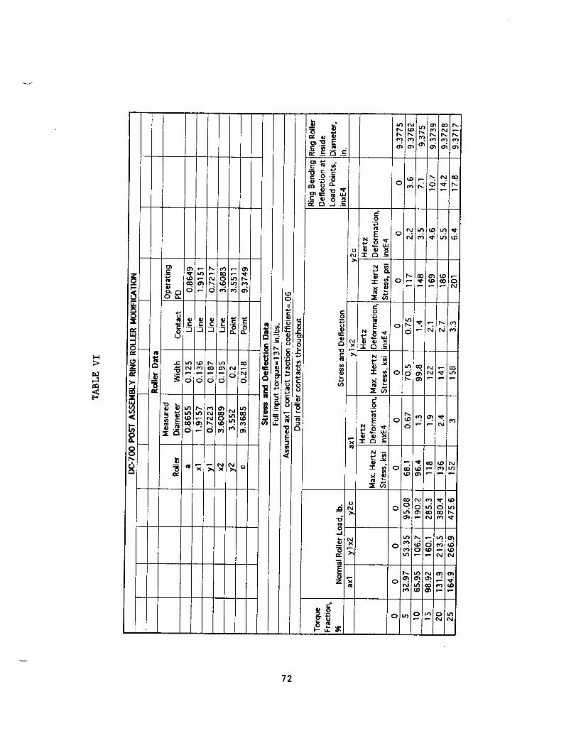
_f
72

I-f:>
r._
_N _ _
_ m m _
0 -- _ _
o _ _
_ x0
73

TABLE VIII
DC-5OO ASSEMBLY
Roller Inspection Data
(ENGLISH UNITS)
Roller Gage Diameters
Sun: a=.8719in.
First Planet: x1=1.8937in.; y1=.7390in.Second Planet: x2=3.0068in.
Roller Serial No. Y Diameter at x= Set No.
x=.340in, x=1.840
Input Sun 0.8711 0.87145
Output Sun 0.871 5 0.871 55
First Planet
Second
Planet-
Stationary
Ring Roller
Numbered Side Rain
x=.150 x=.605 x=.150
1.8938
Side
Second
Planet-
Rotating
Ring Roller
x=.605
0.739351 1.89375 0.73915 1
2 1.8939 0.7393 1.894 0.73915 2
3 1.894 0.73935 1.8938 !0.73915 2
4 1.89385 0.7392
5 1.89375 0.7391
6 1.8939 0.73915
1.89365
1.89385
0.73935
0.73915
2
1.8937 0.73905 Z
7 1.8938 0.7393 1.89375 0.73915 1
8 1.8938 0,7389 1.8938 0.7393 1
Numbered Side Plain Side
x=.265x=.265
1 3.00715 3.00725
2 3.00725 3.0071S
3 3.00735 3.00695
4 3.00675 3.00705
Sho_ end
x=.265
1 3.0066
3
4
3.0073
Long end
x=.265
3.00645
3.00735
3.00735
3.00705
3.0071
3.0068
74

75


0 0
0
_,h _I_ _., _
77

b]
[-,
p_
o_
_,,<1.,-,_.-i ,_ -- _ _il.--_ _ ,,_ ,,-, ,,_,.,-, I_1,,-,_ ,,-i ,-.i ,.-i ,-,i e.,i _,.,i.,,-i ,,-i ,,..,i ..-i ,-.i
^z_ c_z
_1"'""'":" _"___1 _1
"/8

X
!O
0
n
E
LJO0
z_oI--,-
o0It)
6V
_>a
rr"
._J
._.J
o
_>Q
.<
9ILl
.-.I0
_ _ ,w m"
.-_'°d°°°• C_
oo__
0
79

TABLE XII
EFFICIENCY DATA SPECTRA
ANGULAR VELOCITIES, rad./sec
O3Hl
35
70
105
140
35
70
105
140
35
70
105
140
35
7O
105
140
35
70
105
140
U_H2 U_L
35 0
7O 0
105 0
140 0
0 1.2
35 1.2
70 1.2
105 1.2
-35 2.4
0 2.4
35 2.4
70 2.4
-70 3.59
-35 3.59
0 3.59
35 3.59
-105 4.79
-70 4.79
-35 4.79
0 4.79
GREATER OF
toll 1/eL or OH2/mL
oo
oo
oo
oo
R
2R
3R
4R
R/2
R
3R/2
2R
2R/3
2R/3
R
4RJ3
3R/4
R/2
3R/4
R
DIFFERENTIAL
EFFICIENCY, %
0
0
0
0
100
33.3
20
14.3
100
100
5O
33.3
100
100
100
6O
100
100
100
100
80
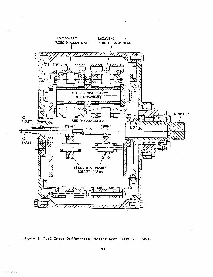
H2SHAFT
STATIONARY
RING ROLLER-GEAR
I
ROTATING
RZNG ROLLER-GEAR
SECOND ROW FLANET
-OL R-GEARS
SUN ROLLER-GEARS
L SHAFT
Hl
SHAFT
FIRST ROW pLANET
ROLLER-GEARS
Figure I. Dual Input Differential Roller-Gear Drive. (DC-700).
81
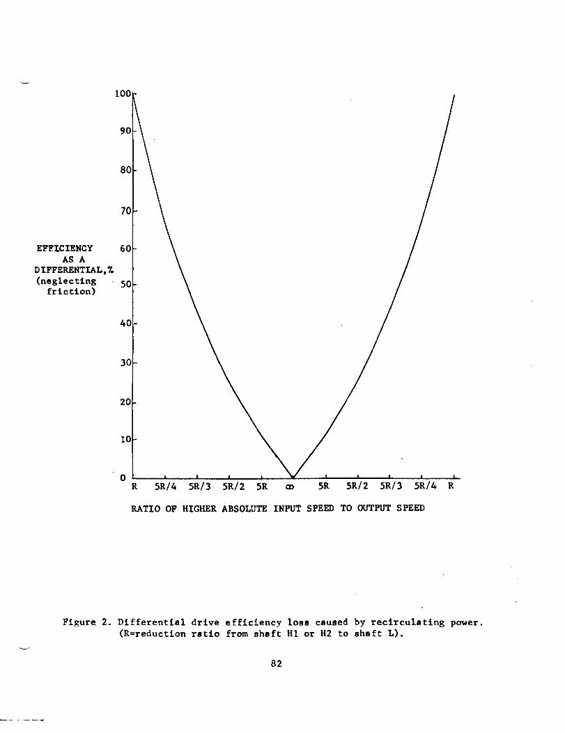
80
70
EFFICIENCY 60
AS A
DIFFERENTIAL,%
(neglecting 50friction)
40
30
20
10
0R 5R/4 5R/3 5R/2 5R ¢D 5R 5R/2 5R/3 5R/4
RATIO OF HIGHER ABSOLUTE INPUT SPEED TO OUTPUT SPEED
R
Figure 2. Differential drive efficiency loss caused by reclrculating power.
(R=reduction ratio from shaft HI or H2 to shaft L).
82

\Gear #16
Rollers
Gear #2
1&2
\
Gear #87&8
Oesr #14
.i14
Ring Oelr
a) Input side cluster
#I
Figure 3. Arrangement of first and second planet roller-gears as viewed
from the input side (DC-700 drive).
83
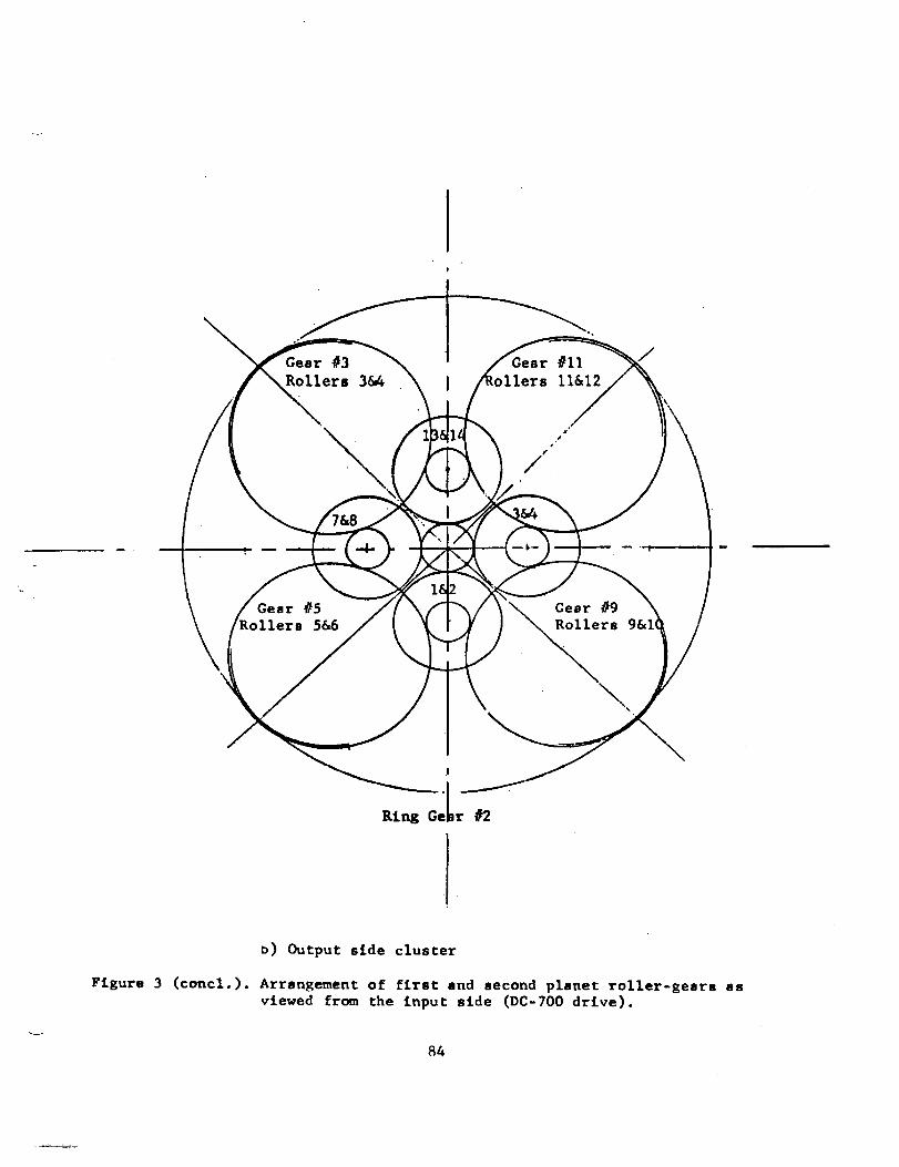
#3 #iiRollers 3&4 _llers ll&12
Gear #9Rollers
v) Output side cluster
Figure 3 (concl.). Arrangement of first snd second planet roller-gears ss
viewed from the input side (DC-700 drive).
84

STATI ONARY ROTATI NG
RING ROLLERS RING ROLLERS
/ tr! _ .'_ ,
,_ _._..__ _ _o_ _,_
-E
21-
L SHAFT
f
_FIRST ROW
PLANET ROLLERS
Figure 4. Dual Input Differential Roller Drive (DC-500).
85

!
CLUSTER
CARRIER
I ,/ 3
ROTATING RING CLUSTER
(View from output side)
4 ./ 1CLUSTER
CARRIER NO.I
STATIONARY CLUSTER
(View from input side)
Figure 5. Arrangement of first and second planet rollers in two cluster
assemblies (DC-500 drive). Viewed from the direction indicated.
86

2.57521ZEROLOAD
2. 5746225?.PRELOAD
2.5744950Z PRELOAD
2. 57428
75?. PRELOAD
1.5034
I. 50311
i. 50294
1.50280
2.57407 1.50268
I00?. PRELOAD
Figure 6. Roller spacing at different levels of preload (DC-500 drive).
87
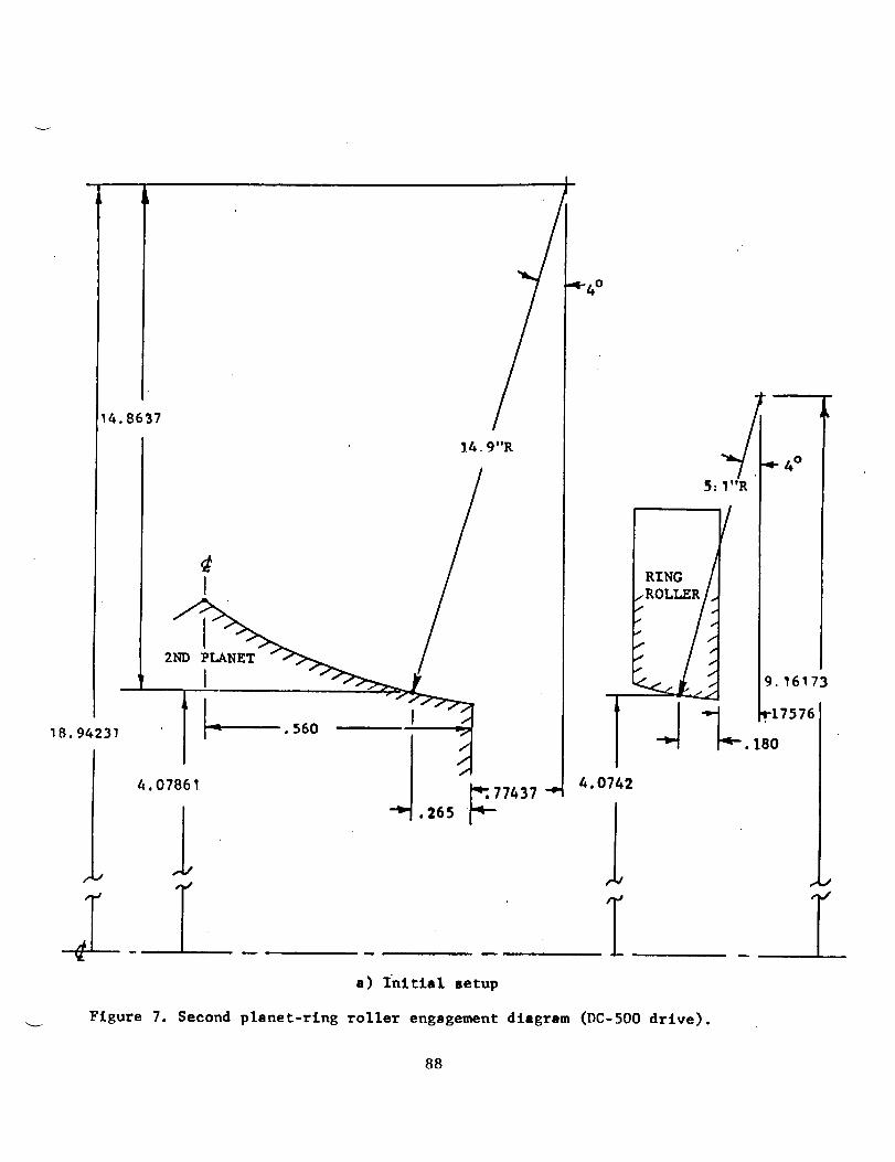
14.8637
18.94231
J
J
14.9"R
2ND PLANET
4. 07861
lT
LI_ .560 ->.
/
q_,77437 "P
"_ . 265
•_-4 o
4.0742
1T
a) Initial setup
I ,5-"I"R
RTNG
/
•w-. 180
Figure 7. Second planet-rlng roller engagement diagram (DC-500 drive).
4°
9.16173
_17576
J
I
88

18.94231-9. 16173
cos 0_- 14.9-5.1
0 i" 3. 60722 °
14. 87048 REF.
1/_. 9'tR
/2
18.94231.
#,
/½
•_ 0 t
I_ .560 wj
d IJ• 16308
#
5. T"R"_ Oj.
RI.o t /
_. T1757614511
4.07183 REF. 'q";77437 "P 4.07183 REF.
9.]6173
b) Zero load engagement point
-Figure 7(cont.) Second planet-ring roller engagement diagram (DC-500 drive).
89

14. 86399
18.94172
cos Of-
!8. 94172-9. 16228
14. 90029.-5. 09971
Of- 3. 76394 °
14.90029
2
w
c) 25"7. preloed
_-4 o
3.76394 °
iI4.07499
1
$
_/ "4 °
5.0997]
3. 76394 ° _/
-'_ 15902
9.16228
_Figure 7(cont.) Second planet-rlng roller engagement
9O
diagram (DC-500 dr£ve).
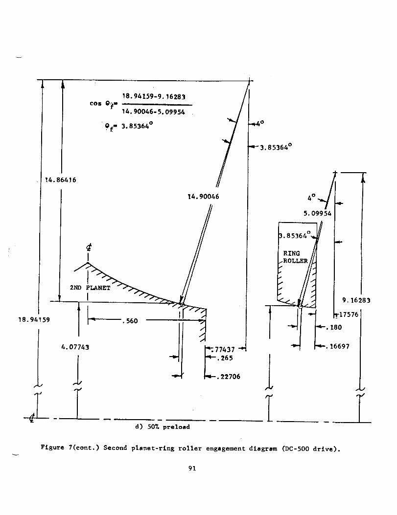
14.86416
18. 94159
"F,_1
cos 0_-
Of-
18.94159-9.16283ii ii iJ ii
14.90046-5.09954
3.85364 °
2ND
r
14. 90046
.560
m
d) 50% preload
4. 07743
T
77437 "*
• 265
.22706
4° d _-
5. 09954
3.85364°_ _
4t_
RING
ROLLER/_
9. 16283
_i .r17576
180
*" 16697
J
Figure 7(cont.) Second planet-r£ng roller engagement dlagram (DC-500 drive).
91

14.86430
18.94138
18. 94138-9. 16338
cos Of ....14. 9006- 5. 09939
Of- 3.94386 °
14.9006
_ 2 .
I _ _
,_._o
•_-.3.94386 °
1lT
45. 09939
0
3. 94386 -_
RING /
ROLLER/_
- //:
H
,q- 4 °
e) 75% preload
9. 16338
"__ 180T17576.17479
Figure 7(cont.) Second planet-rlng roller engagement dlagrsm (DC-500 drive).
92

18.94118
14.86443
cos Of-
18.94118-9.]6393
14.90073-5.09927
Of- 4. 0279 °
14._0073
2ND PLANET
1"!
f) IOOZ preload
"_f 4 °I _"
5.09927
//4. 0279 °
RIs0 /
IROLLE_/
. 180
4.0 _3 _--..18242
.lT
9._6393
Figure 7(concl.) Second planet-rlng roller engagement diagram (DC-500 drive).
93

0.16
0.14
0.12
0.1
0.08
0.06
p. 0.04
0.02
0
0
PRELOAD vs RING ROLLER TRAVEL
r i i i
25 50 75 1 00
PRELOAD,_
Figure 8. Preload level as a £unction of ring roller travel (DC-500 drive).
94

t_
r,_
o<
I
ot_J
n
\\
I I I '
o o oo co r,0f.-
_'av013ucl
\\
\
i x,
o oN
o.o
c5 -
O
d
o
o
!
OO
!
u
v
G
U
m
0
0
0
Law
m
m0
---- g5

IDLER SUN ROLLER_
INPUT SUN
RING ROLLERS
ROW PLANET ROLLER
PLANET CARRIER
(CAGE)
OUTPUT FROM
ROTATING RING
OUTPUT FROM
P.OTATING CAGE
1at ROW PLANET ROLLER
Figure 10. Grounded Ring (Momentum Balanced) Drive (DC-&00).
96

TL2
RING ROLLER
(to shaft L2)
GROUNDED RING
\CAGE
(to shaft LI)
Figure II. Torques snd angular velocities in Grounded Ring 0Momentum Balanced)
Drive (DC-400). Torques are shown as inputted to the drive. Angularvelocities are shown as viewed from one direction.
_ 97
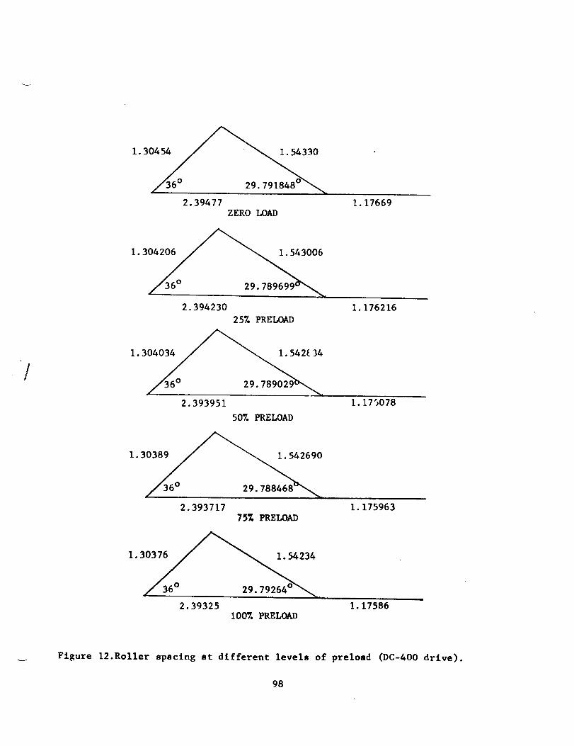
!
I. 30_"
2.39477zERO LOAD
1.17669
I
1.30__
2.39_23025%I_ELOAD
1.176216
I. 175078
2.39395150"/.?RELOAD
1 30_"
2.39371775% ?RELOAD
1.175963
1.3037_
1.17586
2.39325 100% ?RELOAD
Figure 12.Koller spacing at different levels of preload (DC-&O0 drive).
98

8.6
3.5712
//
I
/
/
;iII/
._- 4 °
4- Oi
8.5791
12.1502
.3849
.215
.1284
s) Initial setup, zero load
cos Oi = (12.1502-7.5584)/(8.6-4)
Oi = 3.4216 °
/
/ 4
3. 5682
#/
S
'_ 4 °3.9903
_-Oi
7. 5584
-_-.0990
--'- .180
"_---.1397
1
Figure 13. Second planet-rlng roller engagement diagram (DC-400 drive).
99

/8. 6002
3. 5704
/!/
tl'//
_- 4 °
8. 5793
---. 3849
-.215
--.1646
12. 1497
J
12.1497-7.5587cos e =
8.6002-3.9998
cos 0 = .997957
e = 3.6633 °
_,7,/ / / / /// //
/ 7/
/ 3.9998
3. 5686
.,t.4o
3. 9900
_-O
7.5587
1
'_'-. 0990
q'--. 180
_--.1566
Figure 13(cont.)
b) 25% preload
Second planet-rlng roller engagement diagram (DC-400 drive).
I00

¢
3. 5700
12. 1495
12.1495-7.5589C08 0 =
8.6004-3.9996
cos 0 =.997786
0 = 3.8135 °
3.5690
I
.1670
L
c) 50Z preload
Figure 13(cont.) Second planet-rlng roller engagement diagram (DC-400 drive).
101

P
// _-- 4 °
..,_.. 0
/8. 6005
Y ,
,---. 3849
-'-" //_ .215
_ .2066
,j3. 5697
8.5795
d) 75% preload
12.1492-7.5591CO8 0 ffi
8.6005-3.4995
12. 1492
0
_7/y
/ •
/
//
/ 3. 9995 "/7 / J/
/ //
///
p,,
)694
b
._-4 °
3.9898
_0
7.5591
_- .0990
.180
i
i
.1761
J
Figure 13(cont.) Second planet-rlng roller engagement diagram (DC-400 drive).
102

8.6006R
4 °
8.5797
12. 1488
cos Of = (12.1488-7.5594)/(8.6006-3.9994)
Of = 4.1008 °
o
3. 9897
7. 5594
3. 5691
.3849
.215
,2301
e) Full preload
J , .J_
Figure 13(concl.) Second planet-rlng roller engagement diagram (DC-400 drive).
103

PRELOAD VS RING ROLLER TRAVEL
0.12
0.1
"- 0.08.--I
I--
0.06_1==J0
z 0.04
0.02
0 I I I I
0 25 SO 75 100
PRELOAD,%
Figure 14. Preload level as a function of ring roller travel (DC-400 drive)
104

\
4
View fr_ Input Side
Figure 15. Arrangement of first and second planet rollers as viewed from
the input side (DC-400 drive).
105
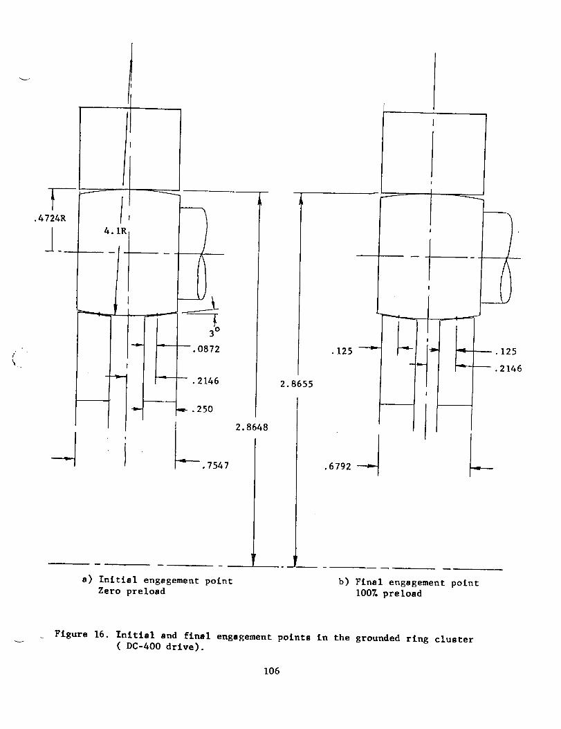
/
.4724R
J_
-- .0872
.2146
.250
2.8648
.7547
a) Initial engagement point
Zero preload
2.8655
i
• 125 _
!!
/f
_!
.125
•2146
b) Final engagement point
100% preload
Figure 16. Initial and final engagement points in the grounded rlng cluster
( DC-400 drive)•
106

_>
IdC3
O g.-I _
J-_ ,I.,I w,4 I-_
•,-_ I.i G
O _U-4 G,,t-I F,-40_1Li._4.) .- . ,_-_ p.IU O O_ C3 m
0
m
m
0
I
O OU
G
mm_
G0
U
MO
0 •M,._ N
0 0 _"
0 0 0
m,_-m
I
I
Ill '
I IJII
1 [IIii ,
I
!¢.)
O
4J
E_
cO
E-_
m
i.-I
w-I
_3
C_O
r'_
107
0
1
I JI!
o
i,,a
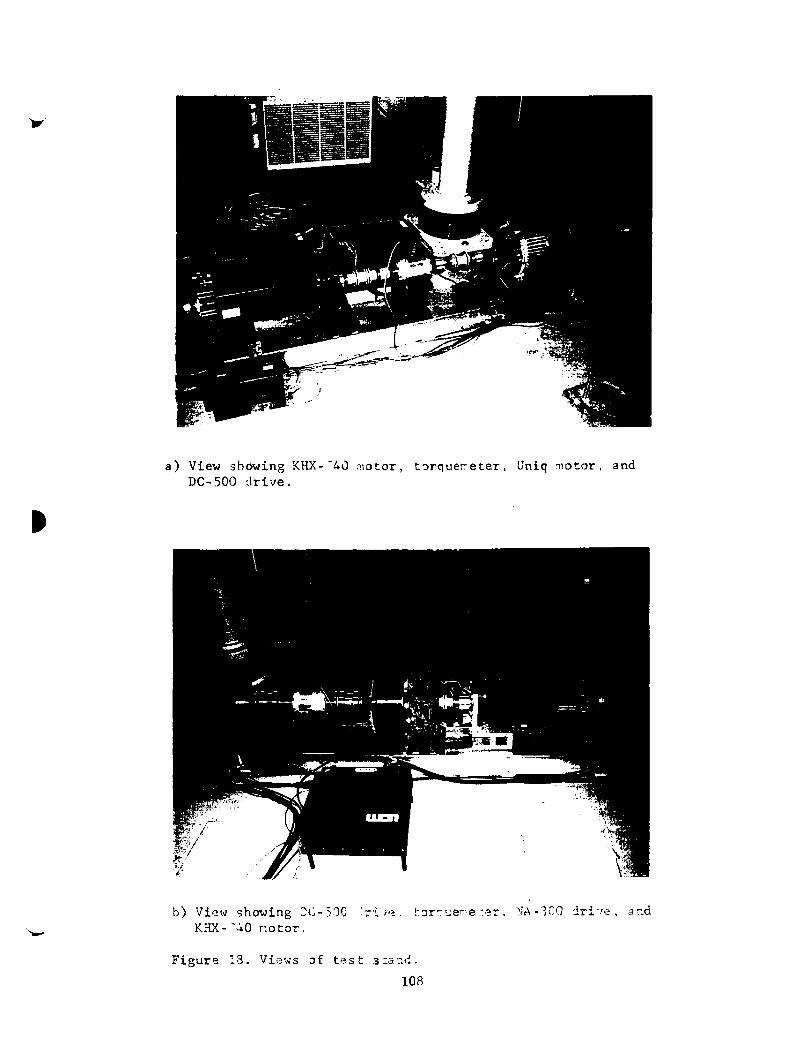
D
a) View showing KHX-_A0 _1otor, t_rque_eter, Uniq motor, and
DC-500 drive.
b) View showing _" 50C ! _ _e '" _" _ -_. _;A '_00 drive, a_.dKHX-"A0 _otor.
Figure 18. Views aftes _ -
108

c) View showing DC-500 drive, torouemeter, and NA-300 drive.
d) View showing Uni_ motor, DC-500 _rive, and tor_:eme'=e':.
Figure l_'cont.). Views of test stand.
109
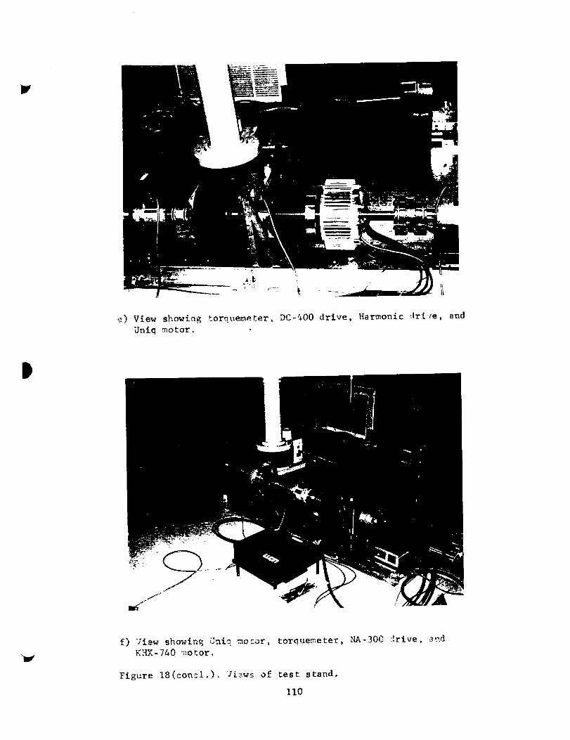
e) View showin_ torquemeter, DC-_O0drive, Harmonic drive, and
Uniq motor.
D
f) View showing Uniq too=or, torque_.eter, NA-30C :[rive, a_,,d
KIiX- 740 _o __or.
Figure 18(concl.). Views of test stand.
II0

29.l
29.4
.o 29.2
"_ 29
28.8
28.6E
28.4
28.;
2E0
m ,! ! | i i ! f
0
. .........
....... ..., .,.,., ,...,, ..,, ,, ,, ,.., .... ,..,,.,,..,., °,.,,.,_ .... °,,,,..,,,,.,,o .... ,...o..,, ....
i
...........I............!.......I'i ..........._............._......................_..........." [' i .........................................
t I I I ! I ! 1
50 100 150 200 250 300 350 400ou_ut (shaft L) angle: ¢legmes
Figure 19. Angular linearlty teat for DC-700. HI driven, H2 fixed,L free.
29.8
0 50 100 150 200 250 300 350 400output (sha_ L) angle: degrees
Figure 20. Repeat of angular llnearity teat of DC-700. H1 driven,
H2 fixed, L free.
III

_ 29.3,5
•_ 29.3
292s
29.2
._ 29.15
2G.1
28.05_
|
J................... """ ................................... i............... "'"; ...............
! ..o°oo,.oH,,° ..... O°H,°,O.°°°,.O°,.,,_,..*°,°.,H., .°,,:°,oo°o,,oo°,°, .°_°,*°°°° °°,o.
i,,,ii,ii.ii.......!I l I I
10 20 30 40 50output (shaft L) angle: degrees
Figure 21. Zoom on 2nd angular llnesrity test for DC-700. HI driven,
H2 £txed, L £ree.
0.8
0.6
0.4
p,.
r--0.2
-0.4
4).6
. I_o
...........i............i..........i...........i............i............i...........i..................... .:............ :..................... .: ............ : ............ } ........... .: ............
l i ! ] ]
...........<......................i...........,.'............:............;...........,.'............
I I I I | I I
-300 -200 -1 O0 0 100 200 300 400Shaft L angle (dew
Figure 22. DC-700 sha£t H1 input cogging torque. H2 £1xed, L £ree.
__ 112
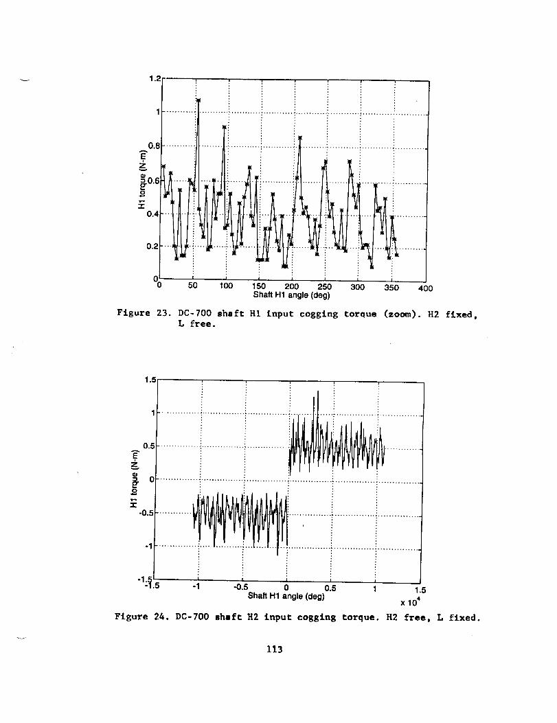
1.2"
1
0.8
0.6o
-r-0.4
0.2
|0(_' I50
= _ = i
I I I I
100 150 200 250 300 350 400Shaft H1 angle (deg)
Figure 23. DC-700 shaft H1 input cogging torque (zoom). H2 fixed,L free.
1.5
,ii iiiiiiiiiiiiii!iiiiiiiiiiiI .............J..............0.5 .............
"" 0 ............... .;................ ! ............... ! ................ _............... ! ................
.. _ i i i1_5 _ _'s ; o's _ 1._
Shaft H1 angle (deg)x 10+
Figure 24. DC-700 shaft H2 input cogging torque. H2 free, L fixed.
113

ZO)
o
1.5 I
O ................................................ _ .................................................
iiiiiii iiiii iiiiiiiilliiiiiiiiiiiii i•0 _t I , I , I I I" " .5 -1 -0.5 0 0.5 1 1.5
Shaft H2 angle (deg) x 104
Figure 25. DC-700 shaft H2 £nput coggir_ torque. HI free, L fixed.
O ........................................................................................
"20 0.5 1 1.5 2 2.5 3 3.5
time (sec)
Figure 26. DC-700 shaft L break-away torque.
114

Zv
= 0
o
-0.1 .............. .:...........................
-0.2:
, ,0 - 1O0 -50I I I
0 50 100H1 speed (rad/sec)
150
Figure 27. DC-700 unloaded drive friction. HI driven, H2 fixed,L free.
0.3
0.2 ..........................................
:
:I I
-1O0 -50
:
! I I
0 50 100H1 speed (rad/sec)
150
Figure 28. DC-700 unloaded drive friction. HI driven, H2 free,L fixed.
115
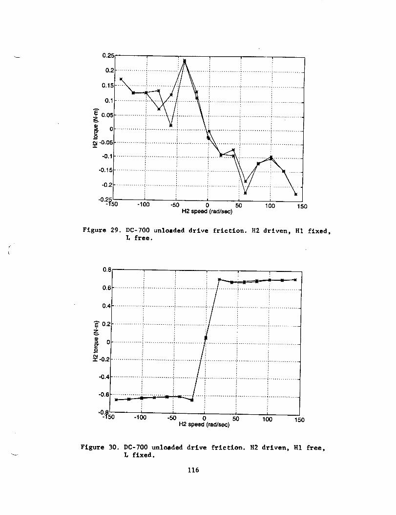
0.; ...........-............
0.15
o1 .........
A
,E0.05 : ...........z¢D
= 0
o
-o.o5
"0._ ................................_..............._......-.....
•................ ................. J..............
....... ! .....
-100 -50 0 50 100 150H2 speed (rad/sec)
Figure 29. DC-700 unloaded drive friction. H2 driven, HI fixed,L free.
0.8 !
0.6
0.4
_" 0.2z
" 0
o
_ -0.2
-0.4
-0.6
-0 i
i
I I I I I
-100 -50 0 50 1O0 150H2 speed (rad/sec)
Figure 30. DC-700 unloaded drive friction, H2 driven, Hl free,L fixed.
116
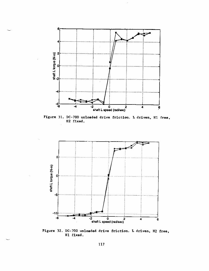
4 ............
_2 ..............z
Q)-I
_'0 ..................
..I
"6-6 -4 -2 0 2 4shalt L speed (ra_sec)
6
Figure 31. DC-700 unloaded drive friction. L driven, H1 free,H2 fixed.
5
-10
-6I
-2 0 2shaft L speed(rad/sec)
4 6
Figure 32. DC-700 unloaded drive friction. L driven, H2 free,HI fixed.
117
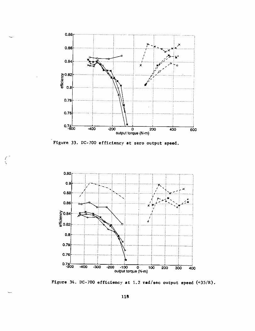
0.88[.............._................i...............i................i ............i................i
0.86J- ............... . ........ : ,_.... :..... "_'_"_ _i ............../ , .._,÷
0.84
_0.82
0.8
0.78
0.76
0.7_ I , I0 400 -200 0 200oulput torque (N-m)
........... . ........... !............................................... i ...........
, : II ! " " ....
................ :............ ................. ,_.............. ,v._ ............. ,................. ,.i : /'i : i
400 600
Figure 33. DC-700 efficiency at zero output speed.
/,
\
0.9
0.88
0.86
>-,
_o.84IlJ
_ o.82
0.8
0.78
0.76
0"7_ 0
0.92 .......... _.......... :.......... : ........................................ !......................
.......... :..,.._,_:_:: ......_.................................... _....! .........._............!/ t -: :.._:
...... .,,. ; .......... _ .......... :.. :,._...... ,_.......... :........... :. ¢ ......... ?.._" ...... :..........
I" : : "_ '. : :I ' E
: : . . I:. _V_.. _. ,• ' " I " os _ _" ' 'S'Yl(
• , . : : _ '. .,- .. ,:...".,_,._. ! .,¢._ .......... _'": .......... : .......... ' ..... " X tTI " _ :
i "_----_:.: ' i ! i :_ ! _" !:: :\: i :_ : :, :
.......__i .................... ; .......... . ......... _:.......... :........... !...........• i i i _i i : :
i ..........i.........................................i
I .... it I l I 1 1 I I
-400 -300 -200 -100 0 100 200 300 400output torque (N-m)
Figure 34. DC-700 efficiency at 1.2 tad/see output speed (+35/R).
118

_,0.88
_0.86
0.84
0.82
°._o
------U._"L......................................... : ..................... ,-...................................
i_ :
0.92 ......... b:; _"-'_: _ "v:2"' '" ' ;; _"..... : .......... :........... :........... :....................... _
--0.9................... _.......... :".......... :"..................... :........... "...................... "
: ..,,t i °_
..........i..........i...................i..........i.:..................i..........:
I I I i I I I I I
-400 -300 -200 -100 0 100 200 300 400output torque (N-m)
Figure 35. DC-700 efficiency st 2.4 rsd/sec output speed (+70/R)
t-
a_ 0.9
0.96 ..................... : ..............................................................................
,,X
• s" •
................... •, ........... _,..-'. ...... ', ................................ .........................
0.94-" _ # - - -_ - - -X_ - - - ._, ,, _ •
0.92 .......... :..........................................................................................
s'*s"
.......... ," ..................... .w" ......... : ................................... _NI - -';" JK .......
• n. ,
0.86
O.R4 I L _ n _ _ _ _
":_;00 -400 -300 -200 -100 0 100 200 300 400output lorque (N-m)
F£gure 36. DC=700 e£fic£eacy at 3.59 rsd/aec output speed (+105/R)
119
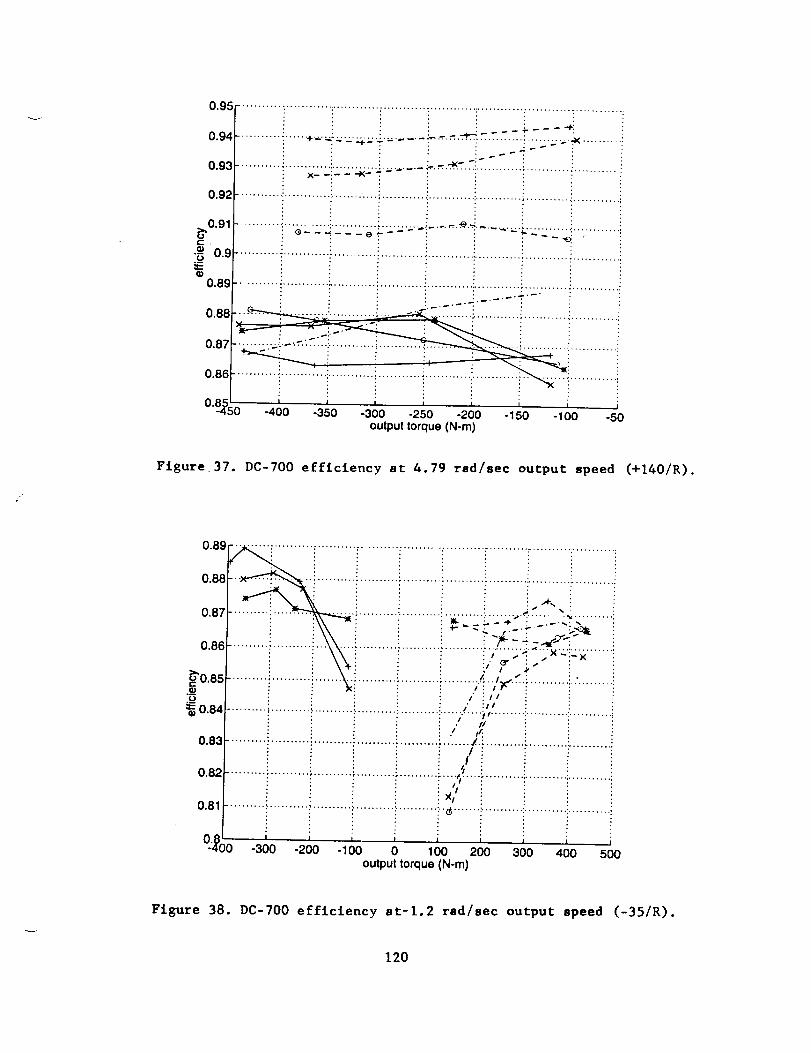
o.9_...........,............:............:...........:............:............::..........._............0.94 .................. +.-_.=:._..-._._--.._.. = .......... .-.._..-..7. ...... : ......... _-._<........... :
0.93 ............................... _- -! - i i iX-- --:-- -- "K--'_'_:"_"--" ":............ :............ _........................ :
0.92 ............ :............ i............ ! ........... _............ :............ i ........... i .............
_.0.91............:............:............:.........._........'_._....................j..E .
° ...........'............:............i i............ii_ 0.9 ....................... ; ........... :............ !
G) : : :
0.89 ......... : ............ .-........... i ........... !............ i............ :........... : ............ i
0.88-.__ ...........___:.-, ......i.....................................;
0.86
8dl_; I I I I I I I •O. 0 -400 -350 -300 -250 -200 -150 -100 -50output torque (N-m)
Figure 37. DC-700 efficiency at 4.79 red/sec output epeed (+140/R).
0.89
0.88
0.87
0.86
_0.85.__¢.)
=_0.84
............ : " : : A "_ •, : ; ........ , ........... ........ ..._. ,, .......... ._ .......... ;........i...... : : .... --; : \,, . . : "_- --'-'." _-"_ i
.......... _ ...... i..._\.. ! ....... i ! _ "_"- _ ;-_'_"3 _ \\i i : :_.....;: _.x._!:_.......: : \_.: • : :/ ¢3" : _* : :
• : : _ 1 _".......... .............................................. • .......... •.......... -.._ - . . .: _:,X : i ..........
. . : ! ,," i/ : :
................... :...... _ ! ! / :_ i
0,83 .........i...............................•..........;..'../ - ....... i
! _ ! i i /! i ! .......i................_ .i ! i _ : !
0.82 . i .......................... _"_............................ :........... ;
0.81.....................;.................: .................._ .......i.................................
-4O0 -300 -200 -1O0 0 100 200 300 400 500output torque (N-m)
Figure 38. DC-700 efficiency at-l.2 rad/sec output epeed (-35/R).
120

0.91F............... i................ i ............... ::............... [ ............................... !
0 " : { : _: " :•91 _ ........_..............i........._<!f .........i................| i ' : _ __:/ :: ;k, J
0.89 ............... _...... _...: ................ !............. 7t.:'_: ......... ! ................ i
. . : :_ ,,_, : .i _: : / ik % i . :>,0.88 ................ :'............. 14 ............... i........... l .... _ i .... _,,L'._..... ........
i _ i 1__"_i_ "-_ i® 0.87 ................................ !_ ............. ! ................ ! .... :,"........ i ................ i
! i i : / ! ii ! : i/ i i
0.86 ........................................ !...............4 ..............................
0.8, _ _ .......!...........{...!...............i................!
i i i 1 i i0. DO -400 -200 0 200 400 600
output torque (N-m)
Figure 39. DC-700 efficiency at -2.4 rad/sec output speed (-701R).
o.92 .................................,.....................i .....................i......................i0.91
0.9
0.89
_088t-
.t! 0.87
0.86
0.85
0.8_
0.83
......... :.......... ! ..........i ..........r............Q;......_........ ..-..........;...........7_i i i i i
-::::i:::::........i..........!.......... ..............f..........i\ .......i..........i..........r..........r..........r;;5-._ .......
.................................................... ; .......... '- .. d.F...-'." . .L ....... ..• : : J , . .
i : : : ._ r _ :. : : : /:1' . . :
.......... ; ................... :. ; • . / . : :
: : : "_...... _.......... :........... :...........! × /: ! i i
.......... _................... i ................... :........ I i ! ! i
.......... , ............................................... #'. ..... [ ........... . .......... : ............
:
:
I I I I I
-300 -200 - 100 0 100 200 300 400 500output torque (N-m)
Figure 40. DC-700 ef£1clency at -3.59 rad/sec output speed (-I051R).
121
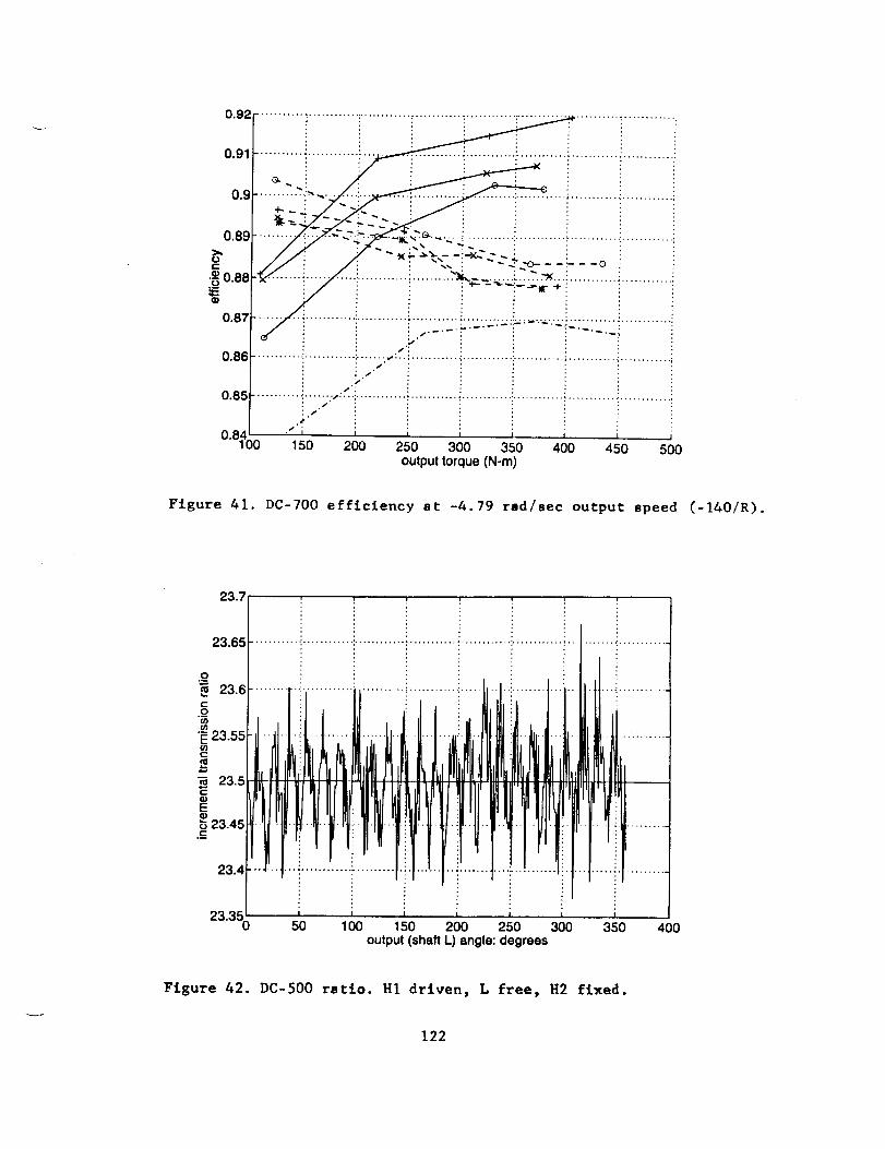
o,21 ii ii .....ii !!!ii i i i iiiiiii0.91__ : '_
o..i , i : : i i i0.9 ........... ,-"--....... :....... ; ........... .......... :............ ; ........... _............
.................. ; ............ i
/J_" __ _-:Xx.--._ i/_: L _''-_--:-^_"-_. _--:- o " "/_ : f'. _" -'_.-'°-_ --i--- : :
................................... " ........................,.,i.- I . _, i_. _._:_; .,i....._... ............................--_' ....... i :
0.86.........................:........:";..........._......................................:...........
•"'; i i ; ; ; i0 84" 100 150 200 250 300 350 400 450 500
output torque (N-m)
0.89
tO=,.-
_ 0.88=::
0.87
Figure 41. DC-700 efficiency at -4.79 radlsec output speed (-1401R).
O
23.6
.=_"_23.55C=
_ 23.5
._ 23.45
23.4
23.350
................i............i............i..........i...........l
I , I I I I L t
50 1O0 150 200 250 300 350 400output (shaft L) angle: degrees
Figure 42. DC-500 ratio. H1 driven, L free, H2 fixed.
122
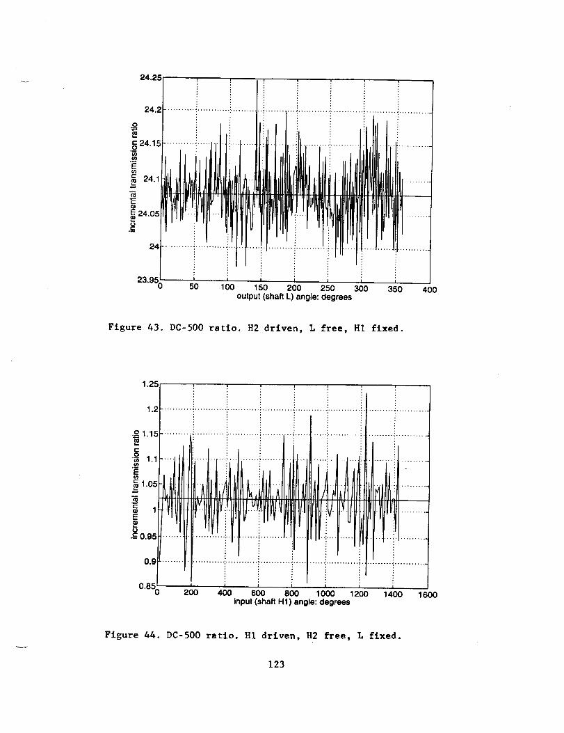
24.;
24
23.! I I I I50 1O0 150 200 250 300 350
output (shaft L) angle: degrees400
Figure 43. DC-500 ratio. R2 driven, L free, HI fixed.
1.2!
0.85200 400 600 800 1000 1200 1400
input (shaft H1) angle: degrees1600
Figure 44. DC-500 ratio. HI driven, H2 free, L fixed.
123
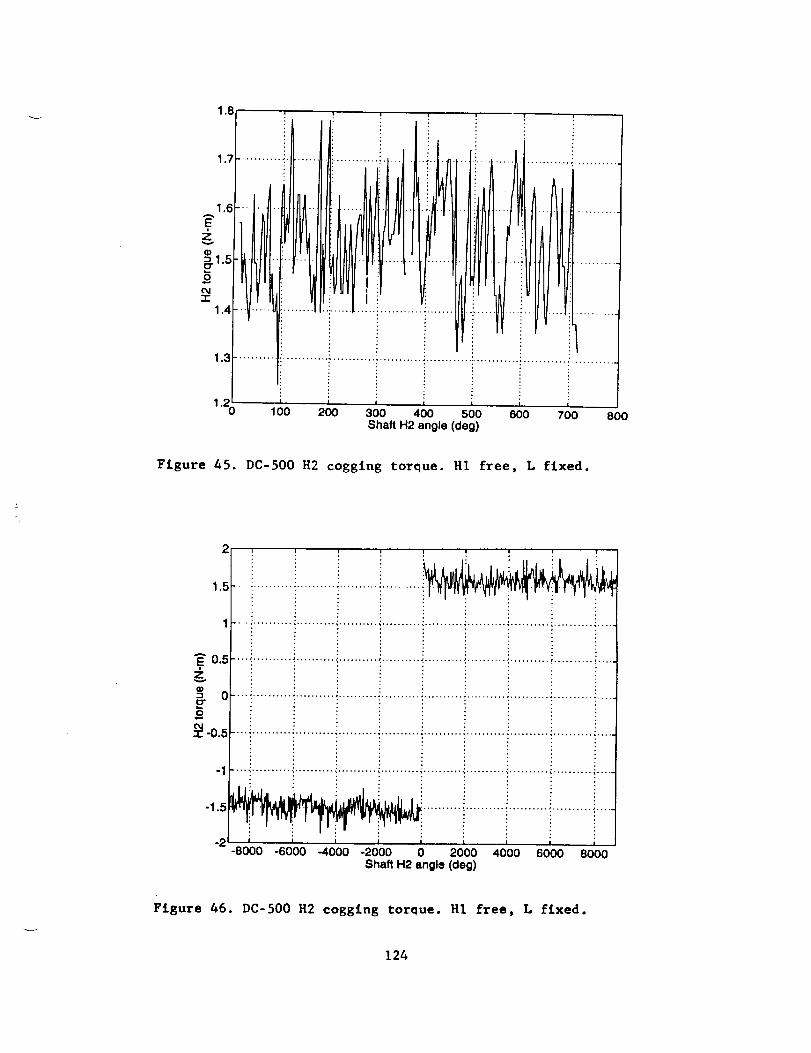
0 I I I I I1. 1O0 200 300 400 500 600 700 800Shaft H2 angle (deg)
Figure 45. DC-500 H2 cogging torque. HI free, L flxed.
2 ! ! ! , , ,
._ 0.5...............................................................................................Z
"_ _ ..._ .......... _..................................................................................
9O4"tin.0. 5 ..., ..................... ,.......... ,.......... ,.......... ,................................ ,.....
-1 ""! .......... ! .......... _.......... _...................................................... i .....
-8000 -6000 -4000 -2000 0 2000 4000 6000 8000Shaft H2 angle (deg)
Figure 46. DC-500 H2 cogging torque. HI free, L fixed.
124

2.5 , , , _ , ,
iiiiiiiiiiiiiiiiiiiiiiiFIIIIIIIII! II1.5
1 ........... :............ :............ :........................ :............ :........................
g 0.5....................................i................................................._............Q)
3Eo 0 ..................................... ; ................................................................
"1""0.5 .......... _............ :...........................................................................
" .............................................J , i i
;00 -300 -200 -100 0 100 200 300 400
Shaft H1 angle (deg)
Figure 47. DC-500 HI cogging torque. H2 free, L fixed.
EZ
Eo
"I-
1.5 , i
1 ........... _............ •............ '........... °......................... '........... °............
0,5 ........... _........................ °..............................................................
-u.o ....................... :..........................................................................
I I I I I I I
:30 -300 -200 -1 O0 0 1 O0 200 300 400Shaft L angle (deg)
Figure 48. DC-500 cogging torque. L free, H2 fixed.
125
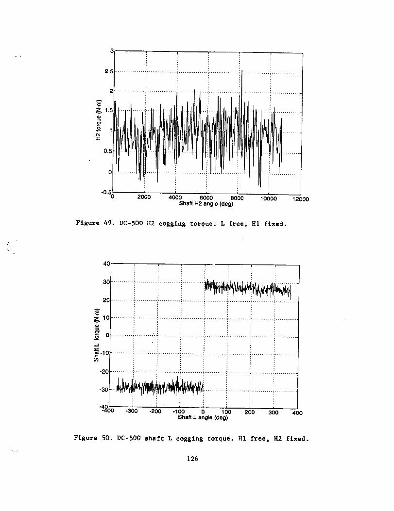
3 , !
Figure 49. DC-500 H2 cogging torque. L free, HI fixed.
f
4O
3O
2O
E
E 0o--I
¢,-if)
-2O
: I
: i
........... .:........................ , ........... .:............ ............. , ........... _..........
,, ,.." , .. ,_.. ,_
i t i I I I
-300 -200 -100 0 100 200 300 400Shaft L angle (deg)
Figure 50. DC-500 shaft L cogging torque.
126
H1 free, H2 fixed.

-350 -300 -250 -200 -150 -100 -50 0ShaftLangle(deg)
Figure 51. DC-500 shaft L cogging torque. H2 free, HI fixed.
151
S1 .............. ":................ , ............... :.............. , ............... i ................
+...o._..............i................+...............i....,E i : : i
_ i :ii. i! ! i i
" 0 ...............:........ " "........: : : .......................
o i :
i i i i1015 .............. _ ................ _ ............... + ................ _ ............... + ................
-', ........................_.-i.... .-
+ + f"1-'_50 -1 O0 -50 0 50 100 151
H1 speed (rad/sec)
Figure 52. DC-500 friction. HI driven, L free, H2 fixed.
127

11l !
I I
-1O0 -50I
0 50 1O0H1 speed (rad/sec)
150
/'
Figure 53. DC-500 friction. HI driven, H2 free, L fixed.
0.8
0.6 ...........
,_ 0.2 ...........................................Z
=_ 0 .........................................................
o
_=_ -0°2 ........................................
-0.4 ............. ,.....
! "
-0.6 ...................................................... _,
-0. s ,0 -100 -50 0 50 100 150
H2 speed (rad/sec)
Figure 54. DC-500 friction. H2 driven, L free, HI fixed.
128

1.5 ............... ! ............ ;:.-:. ............ :................ i ............... _..............
_ _................= : -i................= "_-_.i..............i................_!................i,,._ °_ i ...............i................!................g °...............i.... i...............:...............i..............._...............__ i ! ............... i i
i..............................i iiiiiii.'I................................_. •..............i................i...............i....._,_-_..;._....._...=_....: ....._..
._,; l 50 | ' '- I -100 - 0 50 100 151H2 speed (rad/sec)
Figure 55. DC-500 friction. H2 driven, HI free, L fixed.
30i i
20
.... . ......... "
_ioz=0
,-1
-_o
-20
-3._ I | I i j-4 -2 0 2 4 6
Shaft L speed (rad/sec)
Figure 56. DC-500 friction. L driven, HI free, H2 fixed.
129

151
10
A
E, 5z
Er 0o.J
¢-
-10
i iililiililii iii
"1-56 6I I I ! I
4 -2 0 2 4Shaft L speed (racVsec)
Figure 57. DC-500 friction. L driven, R2 free, HI fixed.
0.6
0.55
0.5
_o.45
_ 0.4
ID
0.35
0.3
0.25
0.2
__.fiR__........... _..................................... _............ :......................................
..........i............i...........i...........i............i...........i...........i............i
......... _......... i............!..........._.............!............!........... _ ........!
V i\\\ i i i i,_i
I i I i I
-300 -200 - 1O0 0 100 200 300 400output torque (N-m)
Figure 58. DC-500 efficiency at zero output speed.
130

0o7 .............. _ ................ ,- ............... _ ................ ." ............... : ................ ;
i i i i i .x :0.6 ............. : ............... ":................ :................ !._'_-_'_ ...... i
• : /// i i io._...............i................_\\_'............?........;_:'....i...............;................io.1...............................i...................::...............................,,'
/
_ ] " I i X I ! I- 0 -200 -100 0 100 200 300output torque (N-m)
Figure 59. DC-500 efficiency st 1.2 rad/sec output speed (+28.8/R).
0.9r ............... :............... ................. :................ : ............... : ................ ;
Lo7L............. :........ _: ........ :............. :......_._..._. :.....
0.6 ........... ..._.'--.._.. ..... i ...... _ ....... _................ _,. ).e.......... _................ i
>, _......_..._,: : v. i I/ : :_o.s-.. ......... _..... •............ r_" ............... ! ................ !® ."_ XiX _ i /t ! i i
i ",,N:\\',i //i i0.3 ..............._ .......... .X.\..\\........_......../,......"...............i................i
! : _ "_ tl : : :o._...............i...................... i.,-.._l........ i ............... i................ i? i \\\ ',- i i
o._................:................:........\_"i":_ ..........:................;................!'k
}(_ | 1 =, I I !- { -200 -100 0 100 200 300output torque (N-m)
Figure 60. DC-500 efficiency st 2.4 red/set output speed (+57.6/R).
131

Figure
I "
-200
xl _."- ..... • ........................................... . .......... :,,/. ....................
I\
._; ............... , ................ :...._ ............ . ............... .• /:/
1 / :1 / :
|
•_l..................I" _...............:...............2
t
..\:..:.........J......-...............................I
: l
! i•!....... _ ........ ,................ =................ j
! _
•
I I 0 I
-100 0 100 200 300output torque (N-m)
61. DC-500 efficiency st 3.59 red/set output speed (+86.2/R).
0.9 ............:.............i .....................":.............":..............!.............
.........................i
0.4............i.............::.............i............._............._.............._...-.,_,.....%
0.3 .......................... :.................................................................. _'"'
O,_5 l l I I I I ,,J0 -300 -250 -200 -150 -1 O0 -50 0output torque (N-m)
Figure 62. DC-500 efficiency at 4.79 red/sec output speed (+II5/R).
132

0.8
0.7
0.6
0,5
=o0.4
0.3
0,9 ............... ";................ : ............... "................ z ............... : .................
:// I• I' 4/ I :
.......i.....J ......i-...............!................i: od ! : :
........ •....j,:........................................]II
0,2 ............... _ ................ • ............. • ................ " ............... ' ................ ,
0.1 ..................................................................................................
_(_ I ,,_ I I I I I- 0 -200 -100 0 100 200 300output torqu_J(N-m)
Figure 63. DC-500 efficiency st -1.2 rad/sec output speed (-28.8/R).
0.9 .............. _................ : ............... _............... : ............... : .... ::_: ........
...:. .............
....................... .....
0o1 .............. ' ..........
-200
[." .................................
I I
-1 O0 0 1 O0 200 300
output torque (N-m)
Figure 64. DC-500 efficiency st -2.4 rsd/sec output speed (-57.6/R).
133
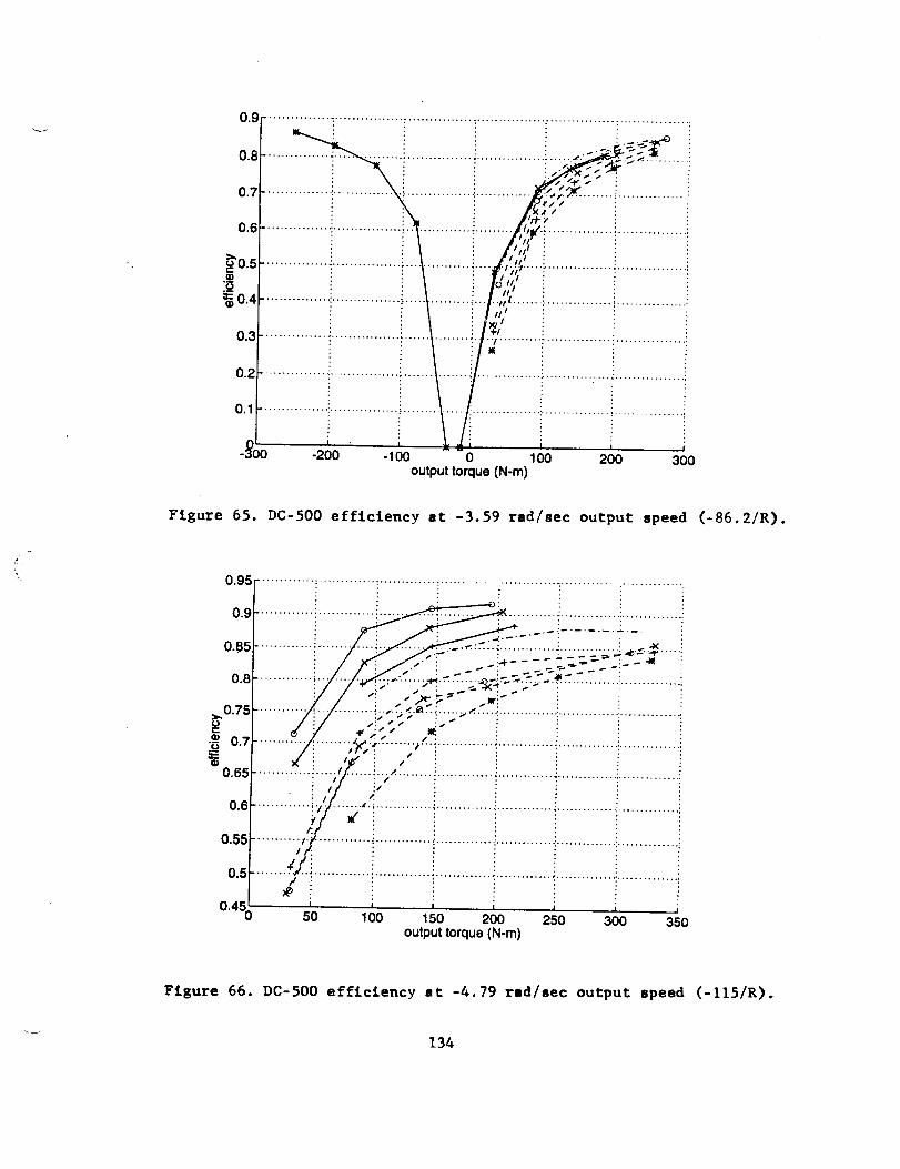
0.9 ............... i ................ ; ............... :................ _............... :.................
_'0.5.__¢3._
=::0.4
0.8 ............... :-..
0.7 ................ :
[--0.6................ :...... .......
0.3 ...........
0.2 ................................ ; ......
0.1 ................ :................ ; ........
- 0 -200 -100 0 100output torque (N-m)
! :
•"i.......................... !................ itl
!
200 300
Figure 65. DC-500 efficiency at -3.59 rad/sec output speed
0.95.............:.............:.............i........................._..............i..............0.9
0..85
0.8
>,0.75
ea•_ 0.7
0.6_
O.I
0.55
0.5
0.450
............. :............._ :..... - __ ........... J.............. !...............
............. i ....... _ ......... _L" _'='=; 3'._= _ ..... i/ F'! /<.-"i .-;-+----z....-- _!---" ;
: _"." ,,/ _'_" :_ : : i
/_._ ._.:._!.............................:..............,: ,.,,: d / :.,,. • : :
............-/_: ........ J" 'i ......... _'"i ...................._:.4............. i:.............. :i.............. !!
............. : ........ /. : ...... : : :: // : / • • ... : ............. : .............. : .............. :
: / :/ : : : :
• : I t. ! : : :............. ;./ ........ ,t. d ............ ; ........... _ ......... : ....... : .... :
_ ! "i ....... : .......... :/: : : i i i
........... I ................ _............. ".............. i.............. :............1/..
.......i......................................................................................xe
i I I I I
50 100 150 200 250 300 350output torque (N-m)
(-86.2/R).
Figure 66. DC-500 efficiency st -4.79 rld/sec output speed (-11SIR).
134

1 i , 1 , i ! t
0.5A
q}
_e
o
° ii
0
_-0.5
0
-1
_ i oo oo1"50 1000 2000 3000 4000 5000 6000 7 0 8 0 9000
input angle H (deg)
Figure 67. Ratio nonlinearity of DC-400. It=LI*R1; tt=L2*R2.
RI=23.98 and R2=24.12 (least squares analysis).
OAR
24.25 ...... . ...... . ...... ...... , ............... ' " -i ...... : ....
i L2 ! i : i
"_ 24.1e,,-,
--_24.05
24.15t-O
i2,23............23.95
.................... :...... : .....b
23'850 1000 2000 3;00 4000 5GlO0 60OO 7000 8000 9000input angle H (deg)
Figure 68. Linearlty test of DC-400. H driven, L1 and L2 free.
135

2 i
1.5 ........................... -_. _
0.5,Ez
0 .................................................. .....
o_"-0.5 ....................... ........... *...... ..... : ..... •.....
-1 ..... i ...... ; ..... i...... '...... _...... i...... i ..... ? ..... '......
-2,.5 i i i i i i i i i-500 -400 -300 -200 -1O0 0 100 200 300 400 500
Shah H angle (deg)
Figure 69. DC-400 shaft H input cogging torque. H driven,L1 and L2 free.
8o
4O
A 2OE
z
0_ 0 ..... , ..... _ ..... • ..... . ..... • ..... ,...... . .... , ..... . .....
i2o/.............................!..............................
6oi ! i!! ! !ot ! z..............................-250 -200 -150 -100 -50 0 50 100 150 200 250
Shah L1 angle (deg)
Figure 70. DC-400 shaft L1 input cogging torque. L1 driven, H and L2 free.
136

-150 -100 -50 0 50 100 150shaft H velocity: rad/sec
Figure 71. DC-400 unloaded ,Irlve friction. H ,!riven, L1 an_ L2 free.
50
40
30
20
_ 10
go"3_ -10
-20
-30
40
-50-5
i i i = i i i i
i; i i i i , , i ,
-4 -3 -2 -I 0 1 2 3 4 5shaft LI velocity: rad/soc
Figure 72. DC-&00 unloaded drive friction. L1 clriven, L2 and H free.
137
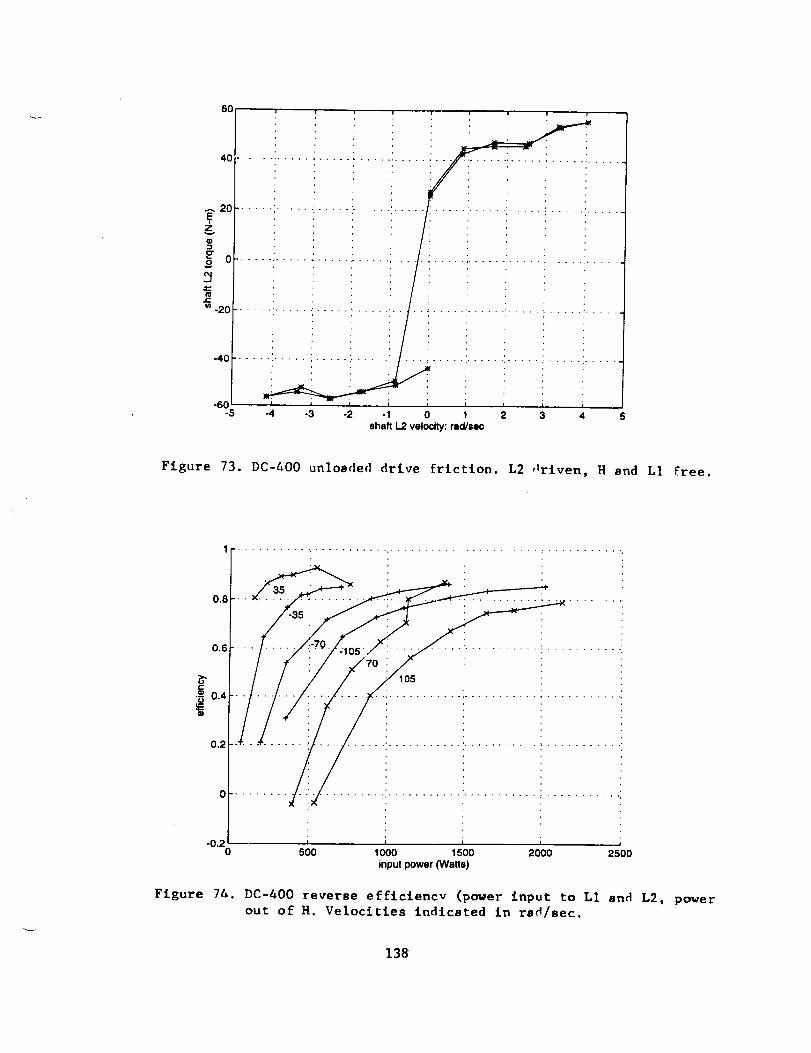
6O
4O
-60-5 -4 -3 -2 -1 0 1 2 3 4 5
shaft L2 velocity: racgsec
_lrivenFigure 73. DC-400 unloaded drive friction. L2 , H 8nd L1 free.
08 i i
•_ 0.4
0.2
0
i L 15'00 ' J-0.20 500 1000 2000 2500
input power (Watts)
Figure 7&. DC-400 reverse efflciencv (power input to L1 and L2, power
out of H. Velocities indiceted in rad/sec.
138

_'0.6c
"0
0.4
0.3
0.2
0.10
0.9 ...... ' 70
o,°_ iiiii
iiiiii200 400 600 800 1000 1200 1400
Inputpower (Watts)
Figure 75. DC-400 Forward efflc£encv (power input to H, power out
of LI and L2).Velocltles indicated in rad/aec
0.8
-0.2-20
0.6
0.4
0.2
i i _ J i
iiiiiiiiiiiiiiiiiiiiiilliiiiiiiiiiiiiiii
-15 -10 -5 0 5 10_ 1'5 20
Input torque: N-m
Figure 76. DC-400 efficiency as a function of input toroue (forward
and reverse operation, with three bidirectional input
speeds). Data from figures 74 and 75.
139

6
5 ....................
z
==4 .........................Eo
¢%
._cC
._2,_>3O"
III
I
0 500 to'oo 1500 20'0o 2500Input power (Watts)
Figure 77. DC-400 shaft H input friction torque loss as a function
of input power. (Computed from reverse efficiency data).
0.85
0.84
0.83
0.82
0.81
_" 0.8
0.7g
0.78
0.77
0.76
0.750.4
i I i J i
• ° • o
I Io8 o18 , 1:2 11,output torque ratio, L1/L2
1.6
Figure 78. DC-400 reverse efficlencv as a function of output torque
ratio TLI/TL2. Shaft H speed, -105 rad/sec.
l&O
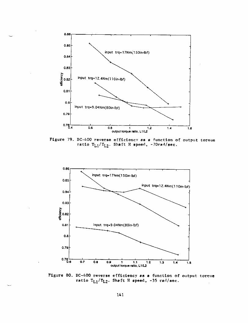
0.88
0.85
0.84
0.83
0c
•_ 0.82_E
0.81
0,8
0.79
0.780.4
i i I i i
_SOin-lbf)
input trq =__
input trq=9.04Nm(8Oin-lbf)
018 018 ; 112 114
output torque ratio, L1/L21.6
Figure 79. DC-&00 reverse efflciencv 8s a function of output toroue
ratio TLI/TL2. Shaft H speed, -70rad/sec.
0.86
0.85
0.84
0.83
i i i i i i i 1
ut trq=17Nm(1 SOin-lbf)
f)
input trq 9.04Nm(8Oin-lbf)
0.82
0.81 _-
o.7_.o oi, ols o'._ ; ,11 t:_ ,:3 1.,'output torque ratio, L1/L2
1.5
Figure 80. DC-400 reverse efficiency as a function of output torque
ratio TLI/TL2. Shaft H speed, -35 rsd/sec.
141

0.96 ......
0.95
0.94
0.93
0.92
_. o.91_1=
0.9
0.88
0.87 inout trq=9.04Nm(8Oin-lbf)
' = ,'.4 ,'.6 1.8°'8%,4 016 0'.8 1 1.2output torque ratio, L1/L2
Figure 81. DC-400 reverse efficiency as s function of output toraue
rstlo TLI/TL2. Shaft H speed, +35 tad/see.
0.96 t i i ! i i i i i
0.94 _-Ibf)
0.92 i.?ut trq=l_. 0.9
¢ 0.88
0.86
0,84
I I
0"8%,8 0,7 01,8 01'9 1 111 112 1'._
output torque ratio, LI/L2
114 115 1.6
Figure 82. DC-400 reverse efficiency as a function of output toroue
ratio TLI/TL2. Shaft H speed,+70 rad/sec.
142

0.93 i i i i i i I i i
0,92 _2.4Nm(1 10in-lbf)
0.91 _n
.0.9
_0.89
Ibf)
0.88
0.87
0'8u.6 0.7 0 8 0.9 1 1 1 1 2 1 3 1.4 1.5 1.6
output torque ratio, L1/L2
Figure 83. DC-400 reverse efflclency as a function of output toraue
ratio TL1/TL2. Shaft H speed, +105 rad/aec.
0.95
0.9
0.85
•-_ 0.8
0.75
0.7
Oin-lbf)
input ,trq= 1 2.4Nm(1 10in-lbf)
0.650.5 2
4Nm(8Oin-lbf)
I I
1 1.5output torque ratio, L1/I..2
Figure 84. DC-400 forwBrd efficiency as a function of output torcue
ratlo TLI/TL2. Shaft R ,,eloclty, +35 rad/aec.
143

0.75
0.7
0.65
., 0.6
0.55
0.5
0.45
0.40.4
i i = i = f
Nm(1 SOin-lbf)
J
J
innut trq=l 2.4Nm(11 Oin-lbf)
input trq=9.04Nm(8Oin-lbf)
o16 o16 ; 11_ ,14 ti6 118 2output torque ratio, L1/L2
2.2
Figure 85. DC-&O0 forward efficiency as a function of output torque
ratio TLI/TL2. Shaft H speed, +70 rad/sec.
0.94
0.93
0.92
_,0.91
_ 0.9
0.69
0.88
J i i i i
ut trq=17Nm(1 50in-lbf)
Oin-lbf)
-,4-
0"87.4 0.6 0 6 1 1 2 1.4 1.6
output torque ratio, L1/L2
Figure 86. DC-400 forward efficiency as a function of output torque
ratio TLI/TL2. Shaft H speed, +105 radlaec.
144

24.2 • i i i i I 1
24 .................................... _ ........................
I
It =
m
23.8 ..................................... •
ii tIE
23.6 ......... _14. . ' ............................. ! ........... i ....."0 M _ ' I_ II
ffl
23.4 ...... - ..... " ......................... . ................. i .....
23.2 ..... , ...... , ................................................
23 i i i i I ¢ I i i
-25( -200 -150 -100 -50 0 50 100 150 200 250
Output (shaft L1) torque: N-m
Fisure 87. DC-400 speed ratio X/L1 as a function of shaft L1 toreue.(Reverse operation as a speed Lncreaser).
145

APPENDICES
APPENDIX A
DUAL INPUT DIFFERENTIAL ROLLER-GEAR DRIVE (DC-700) GEAR DATA
Cluster Geomet_
A cluster geometry that provides easy retrofittability into the Dual Input DifferentialRoller Drive (DC-500) housing with a sun roller amenable to a hollow design with a passthrough quill shaft was sought. The geometry of the Hinge Joint Drive of [5] was suitable. Toreview briefly, the solution from [4]:
_= 18°
(2/5) Nyl = integral number(3/20) Nx2 = integral number
?= 27 °N 1 = 20 teeth_x2 = 100 teeth
Selectinga + Xl = 1.390in(35.306mm)Nx I = 62 teeth
x1 =2.2143in(56.243mm)
Xl = .9576in(24.322mm)
Na = 28 teeth (divisible by 4)xl/a = 62/28 = 2.2142in
(56.243mm)a = 1.390/3.2143 = .4324in
(10.983mm)
Operating P.D. a = .8649in(21.969mm) x1 = 1.9151in(48.644mm)
Selecting a cutter with P = 32 (20 ° pressure angle)Max. permissible Xl OD = 1.9151 + 2(.0188) = 1.9526in(49.596mm)Clearance = 1.9658 - 1.9526 = .0132in(.3353mm)
From eq. (1): (All equations taken from [2] )
(Yl + x2)/(a + Xl) = (sin 45O/sin 27 °) = 1.5575in(39.561mm)Yl + x2 = 2.1650in(54.991mm) x2/Yl =100/20 = 5Yl = .3608in(9.164mm) x2 = 1.8041in(45.824mm)
Operating P.D. Yl = (.3608)(2) = .7217in(18.330mm)
Operating P.D. x2 = (1.8041)(2) = 3.6083in(91.650mm)
Selecting a cutter with P = 28 (20 ° pressure angle)Cutting P.D. Yl = 20/28= .7143in(18.143mm) x2= 100/28= .3.5714in
(90.714mm)
From eq. (2):
z = ((Yl + x2)sin( 90° + ct))/sin 0 = 2.9119in(73.962mm)
Selecting Nc = 264 (divisible by 4)Cutting P.D. c = 264/28 = 9.4286in(239.486mm)
c/x2 = 264/100 = 2.64x2 = 1.7755in(45.099mm)
c - x2 = 2.9119in(73.962mm)c = 4.6874in(119,061mm)
146

Operating P.D. x2 with c gear = 3.551 lin(90.197mm)
Operating P.D. c with x2 gear = 9.3749in(238.121mm)
Ratio = (62/28)(264/20) = 29.23
Gear Stresses (Methods of i61)
Since diametral pitches are in English units, stresses are calculated in English unitsand converted into SI units.
Max. input torque to each sun roller = 15.485Nm(137inlbf)
contacts (4 contacts)
F-r = (137/4)(1/.4324) = 79.21b(352.48N)with face width f = .312in(7.925mm), P = 32, and y = .344
Bending stress, SB = PrP/fY
SB = (79.2)(32)/(.312)(.344) = 23,600psi(162.8x 10⁶pa)
mG = 62/28 = 2.214 (mG+ 1)/raG= 1.45
Compressive stress, Sc = 5715[(FT)(mG + 1)/(mG)(2af)] 1/2
Se = 5715[(Fr)( 1.45)/(2)(.4324)(.312)] 1/2 = 118,500psi(817x 106pa)
2_!x,z.contacts (8 contacts)
Torque = ( 137)(2.214)(1/4) = 75.8inlbf(8.57Nm)
FT= (75.8/2)(1/.361) = 105.11b(467.5N)
Selecting 14.22mm(.56in) face width, P = 28, and y = .33
SB = (105.1)(28)/(.56)(.33) = 15,900psi(109.6x 10⁶pa)
mG= 100/20= 5 (mG+ 1)/mG= 1.2
K = ( 105.1)(1.2)/(2)(.361)(.56) = 312
Se = 57151312] 1/2 = 101,000psi(696x106pa)
x2c contacts (4 contacts)
Torque = 4000inlbf(452Nm)
FT = (4000/4)( 1/4.687) = 2141b(950N)
Selecting 14.22mm(.56in) face width (gear x2), P = 28, and y = .38
147
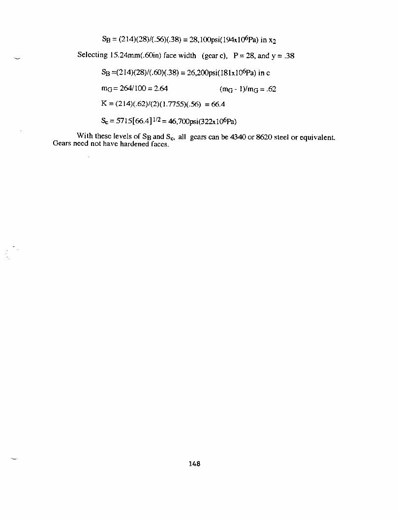
SB = (214)(28)/(.56)(.38) = 28,100psi(194x106Pa) in x2
Selecting 15.24mm(.60in) face width (gear c), P = 28, and y = .38
SB =(214)(28)/(.60)(.38) = 26,200psi(181x 106pa) in c
raG= 264/100 = 2.64 (raG - 1)linG = .62
K = (214)(.62)/(2)(1.7755)(.56) = 66.4
Sc = 5715166.4] 1/Z = 46,700psi(322x 106pa)
With these levels of SB and So, all gears can be 4340 or 8620 steel or equivalent.Gears need not have hardened faces.
148
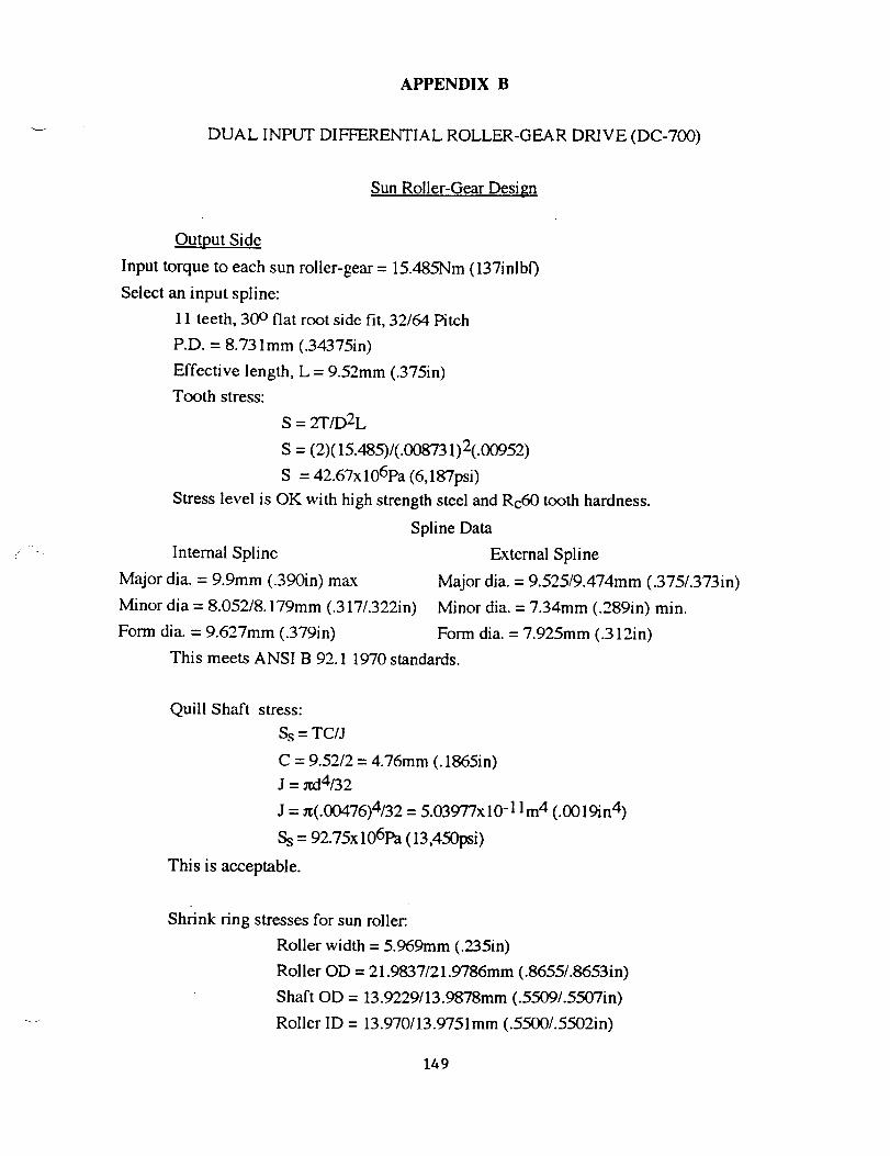
APPENDIX B
DUAL INPUT DIFFERENTIAL ROLLER-GEAR DRIVE (DC-700)
Sun Roller-Gear Design
Output Side
Input torque to each sun roller-gear = 15.485Nm (137inlbf)
Select an input spline:
11 teeth, 30 ° flat root side fit, 32/64 Pitch
P.D. = 8.73 lmm (.34375in)
Effective length, L = 9.52mm (.375in)
Tooth stress:
S = 2T/D2L
S = (2)( 15.485)/(.008731)2(.00952)
S = 42.67x10⁶pa (6,18"/psi)
Stress level is OK with high strength steel and Rc60 tooth hardness.
Spline Data
Internal Spline
Major dia. = 9.9mm (.390in) max
Minor dia = 8.052/8.179mm (.317/.322in)
Form dia. = 9.627mm (.379in)
External Spline
Major dia. = 9.525/9.474mm (.375/.373in)
Minor dia. = 7.34mm (.289in) min.
Form dia. = 7.925mm (.312in)
This meets ANSI B 92.1 1970 standards.
Quill Shaft stress:
Ss = TC/J
C = 9.52/2 = 4.76mm (. 1865in)
J = rtd4/32
,1 = n(.00476)4/32 = 5.039'77x10-1 lm4 (.0019in 4)
Ss = 92.75x10⁶pa (13,450psi)
This is acceptable.
Shrink ring stresses for sun roller.
Roller width = 5.969mm (._5in)
Roller OD = 21.9837/21.9786mm (.8655/.8653in)
Shaft OD = 13.9229/13.9878mm (.5509/.5507in)
Roller ID = 13.970/13.9751mm (.5500/.5502in)
149

Min. dia. interference = .0127mm (.0005in)
Max. dia. interference = .02286mm (.0009in)
Max. ID Shear Stress = Ebd/4r
= (206.9)(.00002286)/(4)(.00699)
=. 169GPa (24,500psi)
Min. fit pressure = Ebd(ro2-ri2)/4ro2a
= (206.9)(.010992-.006992)/4(.01099)2(.00699)
= .056GPa (8,130psi)
Max. fit pressure = (.056)(.02286)/(.0127)
=. 101GPa (14,630psi)
Holding power (coefficient of friction = 0.1)
lAP = miwpf
= n (.00699)(.005969)(.056)(. 1)x 109
= 1,460N (3281b)
Min. torque trans, capability = (HP)(ri)
= (1,460)(.00699)
= 10.2Nm (90.2inlbf)
Req'd. torque to be trans. = (15.485/2)(.2)
= 1.549Nm (13.7inlbf)
M-50 tool steel will be used for the rollers. If they are preheated to 600°F the bore
expansion fir will be
6r = (6.3x 10⁻⁶)(.00699)(600-70)(1000)
= .04572mm (.0018in)
This will be adequate for assembly.
Torsional stiffness of roller-gear and quill shaft
Angle of twist:
0 = TI/GJ
Torsional stiffness
KO = T/O Nm/rad (inlbf/rad)
K0 = GJ/I
For a series of shaft elements:PI
K s ,, G/,_. l, l J,
Refer to Figure 2(b) and (c) for key dimensions
150

For steel
K0 = G/((. 114)/(n/2)(.00952) 2 + (.0533)/(_/2)(.01392-.006352))
= 6.391G Nm/rad (G in Giga Pascals)
= .00039G inlb/rad (G in psi)
G = 82.76Giga Pascals
0 = T/K0
0 = 15.485/(6.391)(82.76)
0 = .02928rad
= 1.68deg
With an assumed backlash of .0508mm (.002in)
0b =.0508/11.11
0b =.00457rad
=.262deg
The "windup" in the output side sun roller-gear will thus be approximately 6 times the
backlash in the sun-first planet mesh. Physically this means that the output speed will
momentarily be slightly different from theoretical.
Input side
Select an input spline
17 teeth, 30 ° flat root side fit, 32/64 pitch
P.D. = 13.494mm (.53125in)
Internal Spline External Spline
Major dia. = 14.656mm (.577in) max Major dia. = 13.919/13.868mm (.5481.546in)
Minor dia. = 12.725/12.852mm(.501/.506in) Minor dia. = 12.090mm (.476in) min.
Form dia. = 14.402mm (.567in) Form dia. = 12.598mm (.496in)
This meets ANS B92.1 1970 spline standards.
Stresses will not be a problem in the spline or the shaft. They are stronger than those
of the output side sun roller-gear.
Torsional Stiffness
Refer to Figure 2(a) fro key dimensions
K0 = G/((.00475)/(_2)(.01212-.00992)
+ (.0667)/(rd2)(.01392-.00992))
K0 = 34.741G Nm/rad (G in Giga Pascals)
= .00212G inlbf/md (G in psi)
151

For steel:
0 = 15.485/(43.741)(82.76)
0 = .00539rad
= .309deg
This is slightly more than the backlash in the sun-first planet mesh. The
consequence of unequal torsional stiffnesses is simply that the output speed will not,
momentarily, be as predicted theoretically. The torsional stiffness of the input side sun roller-
gear could be reduced and made equal to that of the output side sun roller-gear, but there
doesn't seem to be any particular advantage to that.
_- 152

APPENDIX C
DUAL INPUT DIFFERENTIAL ROLLER-GEAR DRIVE (DC-700)
Assembly Procedure
1) Lay Assembly Fixture, DC-700-37, flat on a table.
2) Using Dykem marking compound or equivalent, mark four equally spaced tooth
spaces on the Input Side Sun Roller- Gear Assembly, DC-700-25.
3) Place this Input Side Sun Roller- Gear Assembly on the center post of the
Assembly Fixture and insert the shaft extension of the Input Side Sun Roller-Gear Assembly
into the center post hole. Orient the four equally spaced tooth spaces to face the four equally
spaced holes in the Assembly Fixture.
4) Using the same Dykem marking compound, highlight the indexed tooth
relationship on the large central gear of each of four 1st Row Planet Roller-Gear Assemblies,
DC-700-14.
53 Radially assemble the four 1st Row Planet Roller-Gear Assemblies to the Input
Side Sun Roller- Gear Assembly making sure that each marked index tooth goes into a
marked tooth space on the Input Side Sun Roller- Gear Assembly. Index the Assembly
Fixture on the table so that an Assembly Pin, DC-700-38, can be inserted onto the shaft
extension of each of the 1st Row Planet Roller-Gear Assemblies. This assembled tooth
relationship between the four 1st Row Planet Roller-Gear Assemblies and the Input Side Sun
Roller- Gear Assembly must be maintained.
6) Press fit two Needle Bearings, item 46, into each of four 2nd Row Planet Gears,
DC-700-03.
7) Assemble one 2nd Row Planet Roller, DC-700-01, to each of four 2nd Row
Planet Gears, and fasten in place with Hex Head Screws, item 9.
8) On each of four Planet Shafts, DC-700-31, assemble two Bearing Races, DC-700-
29, one Planet Shaft Spacer, DC-700-02, and one Planet Shaft Key, DC-700-30.
9) Insert each Planet Shaft assembly into a 2nd Row Planet Roller-Gear assembly
with the 2nd Row Planet Roller toward the key end of the Planet Shaft assembly.
10) Radially insert the four Planet Shaft-2nd Row Planet Roller-Gear assemblies into
the four slots of the Assembly Fixture. Each Planet Shaft Key must fit into the key slots on
the Assembly Fixture. Make certain that gears are properly meshed and that proper roller
contact is made.
11) Clamp each Planet Shaft-2nd Row Planet Roller-Gear assembly to the Assembly
Fixture with Planet Shaft Nut, item 44.
12) Assemble two Ring Gear Dowels #1, item 7, and two Ring Gear Dowels #2, item
153
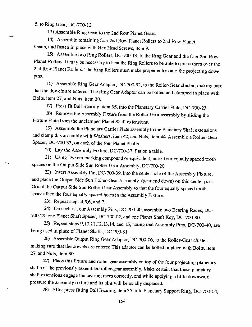
5, to RingGear,DC-700-12.
13)AssembleRing Gearto the2ndRow PlanetGears.
14) Assembleremainingfour 2ndRowPlanetRollersto 2ndRow Planet
Gears,andfastenin placewith HexHeadScrews,item9.
15) Assembletwo Ring Rollers,DC-700-13,to theRingGearandthefour 2nd Row
PlanetRollers. It may be necessary to heat the Ring Rollers to be able to press them over the
2nd Row Planet Rollers. The Ring Rollers must make proper entry onto the projecting dowel
pins.
16) Assemble Ring Gear Adaptor, DC-700-32, to the Roller-Gear cluster, making sure
that the dowels are entered. The Ring Gear Adaptor can be bolted and clamped in place with
Bolts, item 27, and Nuts, item 30.
17) Press fit Ball Bearing, item 35, into the Planetary Cartier Plate, DC-700-23.
18) Remove the Assembly Fixture from the Roller-Gear assembly by sliding the
Fixture Plate from the unclamped Planet Shaft extensions.
19) Assemble the Planetary Carrier Plate assembly to the Planetary Shaft extensions
and clamp this assembly with Washers, item 42, and Nuts, item 44. Assemble a Roller-Gear
Spacer, DC-700-33, on each of the four Planet Shafts.
20) Lay the Assembly Fixture, DC-700-37, flat on a table.
21) Using Dykem marking compound or equivalent, mark four equally spaced tooth
spaces on the Output Side Sun Roller-Gear Assembly, DC-700-20.
22) Insert Assembly Pin, DC-700-39, into the center hole of the Assembly Fixture,
and place the Output Side Sun Roller-Gear Assembly (gear end down) on this center post.
Orient the Output Side Sun Roller-Gear Assembly so that the four equally spaced tooth
spaces face the four equally spaced holes in the Assembly Fixture.
23) Repeat steps 4,5,6, and 7.
24) On each of four Assembly Pins, DC-700-40, assemble two Bearing Races, DC-
700-29, one Planet Shaft Spacer, DC-700-02, and one Planet Shaft Key, DC-700-30.
25) Repeat steps 9,10,11,12,13,14, and 15, noting that Assembly Pins, DC-700-40, are
being used in place of Planet Shafts, DC-700-31.
26) Assemble Output Ring Gear Adaptor, DC-700-06, to the Roller-Gear cluster.
making sure that the dowels are entered.This adaptor can be bolted in place with Bolts, item
27, and Nuts, item 30.
27) Place this fixture and roller-gear assembly on top of the four projecting planetary
shafts of the previously assembled roller-gear assembly. Make certain that these planetary
shaft extensions engage the bearing races correctly, end while applying a little downward
pressure the assembly fixture and its pins will be axially displaced.
28) After press fitting Ball Bearing, item 35, into Planetary Support Ring, DC-700-04,
154

completetheRoller-Gearassemblyby placingWashers,DC-700-34,on theplanetaryshaftextensionsalongwith thePlanetarySupportRing,andclampingin placewith Nuts, item 44.
29) Into the Input Seal & Bearing Carrier, DC-700-28, press fit Seal, item 39, and
install O-Ring, item 36. Grease the O-Ring to facilitate assembly.
30) Into the Input Housing End Plate, DC-700-24, press fit Dowels, item 7,, and
install O-Ring, item 3. Grease the O-Ring to facilitate assembly.
31) Assemble the Input Seal & Bearing Carrier assembly into the Housing End Plate
assembly and fasten with Screws, item 40. Lay this assembly fiat on a table.
32) Take the Roller-Gear assembly and fit it to the Housing End Plate. Make certain
that Ball Beating, item 35, makes proper and full contact with the Input Seal & Bearing
Carrier shaft support, and that the Input Side Sun Roller-Gear Assembly shaft has made
proper entry into the Ring Gear Adaptor.
33) Assemble Main Housing, DC-500-02, to the Input Housing End Plate, and bolt in
place with Bolts, item 1, and Washers, item 2.
34) From the end of the Main Housing surface, measure the distance marked "x" to
the top surface of the Ball Bearing which is press fitted into the Planetary End Plate, DC-700-
04.
35) Into Bearing Cartridge, DC-700-09, asssemble two Ball Bearings, item 24, and
Bearing Spacer, DC-700-11. Insert Output Shaft, DC-700-07, into the Beating Cartridge-
Bearing assembly, and fasten with Bearing Lockwasher and Locknut, items 22 and 23.
Assemble O-Ring, item 26, to the Bearing Cartridge. Grease the O-Ring to facilitate
assembly.
36) Insert this Shaft and Bearing Cartridge assembly into the Output Housing End
Plate, DC-700-05, and assemble O-Ring, item 3, into the End Plate. Grease the O-Ring to
facilitate assembly.
37) From the flange of the Output Housing End Plate, DC-700-05, measure the
distance marked "y" to the shoulder surface on the Output Shaft, DC-700-07.
38) Subtract distance "y" from distance "x" and make Output Shaft Spacer, DC-700-
08, .010 in. less than this determined distance.
39) After push fitting this spacer on the Output Shaft, the Output Housing End Plate
and Shaft Assembly can be fastened to the Main Housing. The spline on the Output Shaft
must make proper entry into the female spline of the Output Ring Gear Adaptor and the
Output Shaft must make proper entry into the Ball Bearing in the Planetary Support Ring.
The Main Housing Bolts and Washer, items 1 and 2, complete the Main Housing assembly.
40) Into Output Seal Carrier, DC-700-10, assemble Seal, item 21, and Gasket, DC-
700-35. Fasten this Seal Carrier Assembly to the Bearing cartridge with Screws, item 20.
41) Install 17.2 oz ( 1.14 pints) of Santotrac 50 fluid after positioning the two pipe
155

plugs ports in the Main Housing on a horizontal centerline.
42) The assembly is completed by inserting two Socket Pipe Plugs, Item 51, into the
Main Housing, and Quill Shaft, DC-700-27, through the Input Side Sun Roller-Gear
Assembly to make spline contact with the Output Side Sun Roller-Gear Assembly.
"- 156

APPENDIX D
DUAL INPUT DIFFERENTIAL ROLLER DRIVE (DC-500)
Assembly Procedure
(Numbers in parentheses refer to callouts on drawing DC-500)
1) Install eight Screw Lock Inserts, (69), into Cluster Carder Sub Assembly, DC-
500-28, (26).
2) Install twenty four Screw Lock Inserts, (53), into Main Housing, DC-500-02, (2).
3) Install six Screw Lock Inserts, (58), into Output Housing, DC-500-10, (7).
4) Install eight Screw Lock Inserts, (83), into Bearing Housing, Input, DC-500-31,
(32).
(32).
(1).
5) Install four Screw Lock Inserts, (79), into Beating Housing, Input, DC-500-31,
6) Install six Screw Lock Inserts, (79), into Housing, Sun Roller Brgs, DC-500-19,
7) Install two Screw Lock Inserts, (51), into Input Housing, DC-500-01, (1).
8) Assemble two J-228 Needle Roller Bearings, (55), into each of four 2nd Row
Planet Rollers, Sta. Ring, DC-500-06, (5).
9) Assemble one 1903S Deep Groove Ball Bearing, (81), and one Snap Ring, (71),
onto Sun Roller, Sta. Ring, DC-500-15 (31).
10) Assemble one 1903S Deep Groove Ball Bearing, (81), and one Snap Ring, (71),
onto Sun Roller, Rotating Ring, DC-500-20, (17).
11) Assemble one 1908S Deep Groove Ball Beating, (59), into Cluster Carrier Plate
A, DC-500-21A, (21A).
12) Assemble one 1908S Deep Groove Ball Beating, (59), into Cluster Carder Plate
B, DC-5OO-21B, (21B).
13) Assemble one 1903H Duplex Ball Bearing Pair, (61), into Housing, Sun Roller
Brgs., DC-500-19, (11). Fasten with Cup Nut, Sun Roller Brgs., DC-500-33, (33). Bearings
are to be installed back to back.
14) Assemble one 1903H Duplex Ball Beating Pair, (61), into Beating Housing,
Input, DC-500-31, (32). Temporarily lock bearings in place by installing Seal Carrier, Input,
DC-500-32, (29) using Socket Head Cap Screws, (78). Bearings are to be installed back to
back.
15) Assemble one 1905S Deep Groove Ball Bearing, (56), and one Snap Ring, (57),
157

into eachof eight Brg. Carriers,2ndRow PlanetRollers,DC-500-03,(6).
16) Assembleone 2nd Row PlanetRoller, Sta.Ring, DC-500-06, (5), onto eachof
four 2nd Row PlanetRoller, Rot. Ring, DC-500-1l, (10). Complete2nd Row Planet Roller
assembliesby installing two of the Step 15 assembliesonto eachof the 2nd Row Planet
Rollers.Fastenin placewith Locknuts,DC-500-09,(8).
17) Start assemblyof the roller clustersby assemblingthe Cluster Carrier Plate
asembliesfrom Steps 11and 12 to Cluster Carrier, DC-500-27,(25). Fastenwith SocketHeadShoulderScrews,(69).
18) Lay theassemblyfrom Step17horizontallyona flat surface.Using .112in. thickwashersasapproximatelocatingspacers,placetwo setsof four 1stRow PlanetRollers,DC-
500-22, (20), into the Cluster Carrier Sub Assembly, moving them radially inward until they
touch (Sun Roller assemblies are not yet installed). Slide four 2nd Row Planet Roller
assemblies from Step 16 into place, mating each bearing Carrier with its guide in a Cluster
Carrier Plate. Position these 2nd Row Planet Roller assemblies solidly against the 1st Row
Planet Rollers. It should now be possible to slip Ring Rollers, DC-500-21B, (21B), andDC-
500-21C, (21C), and Load Rings A, DC-500-26A, (24A), and B, DC-500-26B, (2413) into
place between the 2nd Row Planet Rollers, Rot. Ring, and 2nd Row Planet Rollers, Sta. Ring.
Take care to orient these four parts correctly.
19) Move the four 2nd Row Planet Roller asemblies radially outward against the two
pairs of captured Ring Rollers and Load Rings. Move one set of four 1st Row Planet Rollers
radially outward against the inside diameter of the Cluster Carrier. Insert Sun Roller
assemblies from Steps 9 and 10 into Cluster Carrier, (25). Bring two sets of four 1st Row
Planet Rollers into contact with the Sun Rollers. Bring two sets of four 2nd Row Planet
Roller assemblies into contact with the 1st Row Planet Rollers. It may be necessary to adjust
the axial positions of the two Sun Roller assemblies to establish proper contact. Final
positioning of rollers relative to the Cluster Cartier will not be established until the Ring
Rollers are in position and preloaded.
20) Bring Ring Rollers DC-500-23A, (22A), and DC-500-23B, (22B), into place on
the output side roller cluster. Measure the distance "X" across the outer faces when the
cluster is snugged up. The theoretical nominal dimension is 1.0834in. To apply full preload
the Ring Rollers must approach each other. 144in. from the zero preload position. Calculate
the thickness to grind Preload Fitted Shim, DC-500-23A, (22A), as follows:
Shim thickness = 1.375 -. 187 -. 187 -X +. 144
The nominal theoretical value for the shim thickness is .0834in. After grinding the shim to its
proper thickness, apply preload to the Ring Rollers with C-Clamps until their zero preload
158

distanceX has beenreducedby .144in. AssembleLoad Ring A, Ring Rollers A and B,
PreloadedFitted ShimA, andRing RollerCarrier,DC-500-07,(9), with two Clamping Lugs
A, DC-500-05A, (4A), four Clamping Lugs B, DC-500-05B, (4B), Socket Head Shoulder
Screws, (70), Shoulder Bolts, (3), and Locknuts, (54).
21) Repeat Step 20 for the input side cluster. Assemble Load Ring B, Ring Rollers,C
and D, Preloaded Fitted Shim B, and Grounded Load Ring, Sta. Ring, DC-500-29, (27), with
two Clamping Lugs A, four Clamping Lugs B, Socket Head Shoulder Screws, (70), Shoulder
Bolts, (3), and l_,ocknuts, (54).
22) Assemble Stop Block, Grounded Load Ring, DC-500-30, (28), and Input
Housing, DC-500-01, (1), with two each Socket Head Cap Screws, (74).
23) Assemble Input Housing, DC-500-01, (1), and Bearing Housing, Input, DC-500-
31, (32), with Hex Head Cap Screws, (80), and Plain Washers, (67). "O" Ring, (25), must be
in place and properly greased for assembly.
2,4) Assemble Housing, Sun Roller Brgs., DC-500-19, (11), and Output Spindle, DC-
500-12, (18), using Socket Head Cap Screws, (78).
25) Install one each 1908H Duplex Ball Bearing Pair, (62), with one each Cup Spacer,
Output Brgs., DC-500-13, (14), and one each Cone Spacer, Output Brgs., DC-500-14, (15),
into Output Housing, DC-500-110, (7). Lock the bearings temporarily in place with Seal
CArrier, Output, DC-500-16, (16), and Cap Screws, (66). Insert the assembly from Step 24,
disassemble Seal Carrier, Output, (16), install Locknut, (64), and reassemble Seal Carrier,
Output, (16). Measure the distance "Y" on this assembly.
26) Lay the assembly from Step 23 on parallel bars with the input side face of the
Input Housing down. Carefully mate the roller cluster assembly from Step 21 with the Input
Housing assembly. The Sun Roller, Sta. Ring, must enter the Stop Block, Grounded Load
Ring, (28).
27) Assemble the Main Housing, DC-500-02, (2), and the assembly from step 26 with
Hex Head cap screws, (72), and Plain Washers, (73). Make certain that "O" Ring, (52), is in
place and properly greased for assembly. Measure distance "Z" from the face of the Main
Housing to the inner race face of the 1908S Ball Bearing in Cluster Carrier Plate A. Grind the
Fitted Spacer, Cluster Carrier Brg., (34), to a thickness T, where
T =Z- Y -.078
This will insure that the Wave Spring, (60), is compressed to its proper working height of
.078in.
28) Disassemble Seal Carrier, Output, (16), Locknut, ((64), Output Housing, (7),
Output Spindle, (18), and Housing, Sun Roller Brgs, (11).
159

29) PlaceWave Spring,(60),andFitted Spacer,(34), on Housing,SunRoller Brgs.,
(11).Assembleonto SunRoller, RotatingRing, (17),andinto 1908SBall Bearing in Cluster
CarrierPlateA, (21A). RemoveCupNut, (33), installLocknut,(12), reinstall Cup Nut, (33),
and install Jam Nut, Sun Roller Brgs., DC-500-08, (13). Assemble Output Spindle, (18), with
Socket Head Cap Screws, (78), making certain that splines engage properly. Assemble
Output Housing, (7), with Hex Head Cap Screws, (72), and Plain Washers, (73). Make
certain that "O" Ring, (52), is in place and properly greased for assembly.
30) Disassemble Seal Carrier, Output, (16). Install Locknut, (64). Assemble Seal
Cartier, Output, (16), with Seal, (65), and "O" Ring, (63). Make certain that the "O" Ring is
properly greased for asembly. Install this assembly with Hex Head Cap Screws, (66), and
Plain Washers, (67).
31) Remove Seal Carrier, Input, (29). Install Locknut, (12). Assemble "O" Ring, (76),
properly greased for assembly, and Seal, (77), into Seal Carrier, Input, (29). Install this
asembly using Socket Head Cap Screws, (78).
32) Install 31.4 oz ( 2.1 pints) of Santotrac 50 fluid after positioning the two pipe plug
ports in the Output Housing on a horizontal centerline.
33) Install two Socket Pipe Plugs, (82). Use nylon pipe thread sealer on each plug.
160

APPENDIX E
GROUNDED RING (MOMENTUM BALANCED) DRIVE (DC-400)
Assembly Procedure
( Cailouts on drawing DC-400 correspond to part numbers))
1904H
fit into
Output
7.
1) Lap the .7874" diameter on Sun Roller, DC-400-31, for an easy push fit into
Angular Contact Bearings, Part 69.
2) Lap the 1.1811" diameter on Output Spindle, Inner, DC-400-16, for an easy push
1906H Angular Contact Beatings, Part 60.
3) Install twenty Screw Lock Inserts, Part 82, in Main Housing, DC-400-2.
4) Install six Screw Lock Inserts, Part 84, and five Screw Lock Inserts, Part 54, in
Housing, DC-400-8.
5) Install four Screw Lock Inserts, Part 81, in Input Housing, DC-400-1.
6) Install ten Screw Lock Inserts, Part 82, in Grounded Ring, DC-400-3.
7) Install five Screw Lock Inserts, Part 65, in Cluster Carrier, DC-400-25.
8) Install ten Screw Lock Inserts, Part 68, in Idler Cluster Retaining Ring, DC-400-
9) Install one Needle Roller Bearing, Part 79, in each of five Front Bearing Carriers,
2rid Row Planet, DC-400-4.
10) Install one Needle Roller Bearing, Part 53, in each of five Rear Beating Carriers,
2rid Row Planet, DC-400-10.
11) Install one Needle Roller Beating, Part 64, in Output Spindle, Inner, DC-400-16.
12) Assemble two Retaining Rings, Part 52, one Planet Roller, 2nd Row, DC-400-7,
and two Keys, 2nd Row Planet Roller, DC-400-36, on each of five Shafts, 2nd Row Planet,
DC-400-11. Measure the gap between the 2nd Row Planet face and the Retaining Ring on the
short side of the shaft. Grind each of five Fitted Spacers, 2nd Row Planet, DC-400-21, for a
no shake fit. (The nominal thickness is .050"). Install the Retaining Ring, and mount the
Bearing Carriers from steps 9 and 10 to complete the 2rid Row Planet Roller assemblies.
13) Install two 1906H Angular Contact Bearings, Part 60, Cup Spacer, Inner Output
Bearings, DC-400-13, Cone Spacer, Inner Output Bearings, DC-400-14, and Retaining Ring,
.Part 57, into Output Spindle, Outer, DC-400-20. Beatings are to be installed back to
back.Measure the gap between the bearing face and the Retaining Ring. Grind Fitted Cup
Spacer, Inner Output Bearings, DC-400-35, for a no shake fit. (The nominal thickness is
.066"). Remove Retaining Ring, Part 57, install the Fitted Cup Spacer, and reinstall the
Retaining Ring. Install Retaining Ring, Part 58.
161
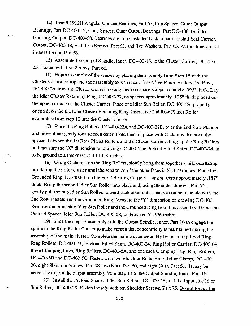
14) Install 1912H Angular Contact Bearings, Part 55, Cup Spacer, Outer Output
Bearings, Part DC-400-12, Cone Spacer, Outer Output Bearings, Part DC-400-19, into
Housing, Output, DC-400-08. Bearings are to be installed back to back. Install Seal Carrier,
Output, DC-400-18, with five Screws, Part 62, and five Washers, Part 63. At this time do not
install O-Ring, Part 56.
15) Assemble the Output Spindle, Inner, DC-400-16, to the Cluster Carrier, DC-400-
25. Fasten with five Screws, Part 66.
16) Begin assembly of the cluster by placing the assembly from Step 15 with the
Cluster Carrier on top and the asssembly axis vertical. Insert five Planet Rollers, 1st Row,
DC-400-26, into the Cluster Carrier, resting them on spacers approximately .095" thick. Lay
the Idler Cluster Retaining Ring, DC-400-27, on spacers aproximately. 125" thick placed on
the upper surface of the Cluster Carrier. Place one Idler Sun Roller, DC-400-29, properly
oriented, on the the Idler Cluster Retaining Ring. Insert five 2nd Row Planet Roller
assemblies from step 12 into the Cluster Carrier.
17) Place the Ring Rollers, DC-400-22A and DC-400-22B, over the 2nd Row Planets
and move them gently toward each other. Hold them in place with C-clamps. Remove the
spacers between the 1st Row Planet Rollers and the Cluster Carrier. Snug up the Ring Rollers
and measure the "X" dimension on drawing DC-400. The Preload Fitted Shim, DC-400-24, is
to be ground to a thickness of 1.013-X inches.
18) Using C-clamps on the Ring Rollers, slowly bring them together while oscillating
or rotating the roller cluster until the separation of the outer faces is X-. 109 inches. Place the
Grounded Ring, DC-400-3, on the Front Bearing Carriers using spacers approximately. 187"
thick. Bring the second Idler Sun Roller into place and, using Shoulder Screws, Part 75,
gently pull the two Idler Sun Rollers toward each other until positive contact is made with the
2nd Row Planets and the Grounded Ring. Measure the "Y' dimension on drawing DC-400.
Remove the input side Idler Sun Roller and the Grounded Ring from this assembly. Grind the
Preload Spacer, Idler Sun Roller, DC-400-28, to thickness Y-.576 inches.
19) Slide the step 13 assembly onto the Output Spindle, Inner, Part 16 to engage the
spline in the Ring Roller Carrier to make certain that concentricity is maintained during the
assembly of the main cluster. Complete the main cluster assembly by installing Load Ring,
Ring Rollers, DC-400-23, Preload Fitted Shim, DC-400-24, Ring Roller Carrier, DC--400-09,
three Clamping Lugs, Ring Rollers, DC-400-5A, and one each Clamping Lug, Ring Rollers,
DC-400-5B and DC-400-5C. Fasten with two Shoulder Bolts, Ring Roller Clamp, DC-400-
06, eight Shoulder Screws, Part 78, two Nuts, Part 50, and eight Nuts, Part 51. It may be
necessary to join the output assembly from Step 14 to the Output Spindle, Inner, Part 16.
20) Install the Preload Spacer, Idler Sun Rollers, DC-400-28, and the input side Idler
Sun Roller, DC-400-29. Fasten loosely with ten Shoulder Screws, Part 75. Do not torque the
162

screws tightly.
21) Assemble Housing, Input, DC-400-01, and Grounded Ring, DC-400-03, with ten
O-Rings, Part 77, in place (properly greased), ten Cap Screws, Part 76, and ten Washers, Part
63. Install 1904H Angular Contact Bearings, Part 69. Bearings are to be installed face to face.
Install Seal Carrier, Input, DC-400-32, using four Screws, Part 72, and four Washers, Part 73.
At this time do not install O-Ring, Part 70, or Rotary Seal, Part 71.
22) Place the assembly from step 21 on blocks about 2" thick, with the input side face
down. Join the assembly from steps 19 and 20, by inserting the Sun Roller into the 1904
Angular Contact Bearings, and the five Second Row Planet Roller Shafts inside the
Grounded Ring. Turn the assembly over and remove the Seal Carrier, Input, DC-400-32.
Install Locknut, Input Bearing, DC-400-30. Install O-Ring, Part 70, properly greased, in Seal
Carrier, Input. Reinstall the Seal Carrier, Input, into Housing, Input.
23) Install one each O-Ring, Part 80, properly greased, into Housing, Input, (step 21
assembly) and Housing, Output, (step 14 assembly).
24) Join the input assembly from steps 21, 22 and 23 with the Main Housing, DC-4OO-
02. Fasten with Screws, Part 67, and Washers, Part 63.
25) Join the output assembly (steps 14 and 23) with the Main Housing. Remove Seal
Carrier, Output, and install Locknut, Outer Output Bearings, DC-400-15. Install O-Ring, Part
56, properly greased, in Seal Carrier, Output, and reinstall into Housing, Output.
Fasten with Screws, Part 67, and Washers, Part 63. Install Locknut, Inner Output Bearings,
DC-400-17.
26) Apply torque to Idler Sun Roller Shoulder Screws, Part 75, using the access ports
in the Input Housing. Torque each screw sequentially. Rotate or oscillate the drive while
torqueing, until each screw is solidly bottomed. Check for smooth, counterrotation of the
outputs when the Sun Roller is rotated. Install ten Socket Pipe Plugs, Part 74. Use nylon pipe
thread sealer on each plug.
27) Install Rotary Seals, Parts 59, 61, and 71..
28) Install 18 oz ( 1.2 pints) of Santotrac 50 fluid after positioning the two pipe plug
ports in the Output Housing on a horizontal centerline. Install two Pipe Plugs, Part 83. Use
nylon pipe thread sealer on each plug.
-.-- 163