Top Arm Identification in Multi-Armed Bandits

with Batch Arm Pulls

Kwang-Sung Jun Kevin Jamieson Robert Nowak Xiaojin Zhu

UW-Madison UC Berkeley UW-Madison UW-Madison

Abstract

We introduce a new multi-armed bandit(MAB) problem in which arms must be sam-pled in batches, rather than one at a time.This is motivated by applications in socialmedia monitoring and biological experimen-tation where such batch constraints naturallyarise. This paper develops and analyzes al-gorithms for batch MABs and top arm iden-tification, for both fixed confidence and fixedbudget settings. Our main theoretical re-sults show that the batch constraint does notsignificantly a↵ect the sample complexity oftop arm identification compared to uncon-strained MAB algorithms. Alternatively, ifone views a batch as the fundamental sam-pling unit, then the results can be interpretedas showing that the sample complexity ofbatch MABs can be significantly less thantraditional MABs. We demonstrate the newbatch MAB algorithms with simulations andin two interesting real-world applications: (i)microwell array experiments for identifyinggenes that are important in virus replicationand (ii) finding the most active users in Twit-ter on a specific topic.

1 Introduction

We consider the top-k pure-exploration problem forstochastic multi-armed bandits (MAB). Formally, weare given n arms that produce a stochastic rewardwhen pulled. The reward of arm i is an i.i.d. samplefrom a distribution ⌫i whose support is in [0, 1]. Thebounded-support assumption can be generalized to the�-sub-Gaussian assumption. Denote by µi = EX⇠⌫

i

Xthe expected reward of the arm i. We assume a uniquetop-k set; i.e., µ

1

� µ2

� ... � µk > µk+1

� ... � µn.

In this work, we introduce a new setting in whicharms must be pulled in batches of size b. We also

Appearing in Proceedings of the 19th International Con-ference on Artificial Intelligence and Statistics (AISTATS)2016, Cadiz, Spain. JMLR: W&CP volume 51. Copyright2016 by the authors.

consider the additional constraint that any one armcan be pulled at most r b times in a batch(if r = b then there is no constraint). Said an-other way, the action space is defined as A :={a 2 {0, 1, . . . , r}n |

Pni=1

ai b}, where a 2 A indi-cates the number of arm pulls for each arm. Wecall this the (b, r)-batch MAB setting. Note that thisencompasses the standard MAB setting, which cor-responds to b = 1, r = 1. The general (b, r)-batchsetting is fundamentally di↵erent, since sampling de-cisions must be made one batch at a time, rather thanone sample at a time. This loss in flexibility couldhinder performance, but our main theoretical resultsshow that in most cases there is no significant increasein sample complexity.

There are many real-world applications where thebatch constraint arises. For example, suppose thearms represent Twitter users and the goal is to findusers who tweet the most about a topic of interest. Us-ing Twitter’s free API, one can follow up to b = 5000users at a time, which amounts to a batch of that size.Also, a user is either observed or not, so r = 1 inthis application. The batch is the fundamental sam-pling unit in such applications, and thus this paperis interested in methods that aim to reduce the batchcomplexity : the total number of batches, or rounds,to correctly identify the top-k arms. As another ex-ample, we consider the problem of using microwell ar-ray experiments to identify the top-k genes involvedin virus replication processes. Here the arms are genes(specifically single knockdown cell strains) and a batchconsists of b = 384 microwells per array. In this case,we may repeat the same gene (cell strain) in every mi-crowell, so r = 384.

Returning to the discussion of theory and algorithms,we consider two settings: fixed confidence and fixedbudget. In the fixed confidence setting, given a targetfailure rate � the goal is to identify the top-k armswith probability at least 1�� using the fewest possiblenumber of batches. In the fixed budget setting, givena budget number of batches B, the goal is to identifythe top-k arms with as high probability as possible.For the fixed confidence (budget) setting, we propose

Top Arm Identification in Multi-Armed Bandits with Batch Arm Pulls

the BatchRacing (BatchSAR) algorithm and prove itstheoretical guarantee in Section 3 (Section 4). Ouranalysis shows that batch MABs have almost the samesample complexity as unconstrained MABs as long asr is not too small relative to b.

An alternative to our batch MAB algorithms is to usestandard MAB algorithms as follows. One could useeach batch to obtain a sample from a particular armof interest, and e↵ectively ignore the rest of the datafrom each batch. This would allow one to use standardMAB algorithms. For example, in the Twitter appli-cation we could follow just one user at a time while wecan follow 5000 for the same cost (free). Our resultsshow that in most cases this (obviously naive) reduc-tion to the standard MAB would have a batch com-plexity b times greater than that of our batch MABalgorithms.

In section 5, we validate the analysis of the proposedalgorithms with a toy experiment, and evaluate the al-gorithms on real-world data from the two applicationsintroduced above.

2 Related Work

The pure exploration problem in MAB has a longhistory dating back to the ’50s with the work of [4]and [20]. The top-k exploration, or subset selection,in stochastic MAB has received much attention re-cently. In the fixed confidence setting including theProbably Approximately Correct (PAC) setup, theRacing algorithm for the top-1 exploration problemwas proposed by Maron and Moore [19] and by Even-Dar et al. [6] independently. The Racing algorithmperforms uniform sampling on surviving arms whiledeactivating infeasible arms based on confidence in-tervals. Racing was generalized to top-k identifica-tion by Heidrich-Meisner and Igel [9], and its samplecomplexity was analyzed in [17]. Median Elimination(ME) [6, 14] runs in stages where each stage eliminatesthe bottom half of the surviving arms. Under the PACsetup, the sample complexity of ME matches the lowerbound. Going beyond elimination-based algorithms,LUCB proposed by Kalyanakrishnan et al. [15] adap-tively chooses which arm to pull based on confidenceintervals without explicitly removing arms. Kaufmannet al. improved both Racing and LUCB with confi-dence intervals based on Cherno↵ information, thoughrestricted to exponentially distributed rewards [17].

In the fixed budget setting, Successive Accepts andRejects (SAR) proposed by Bubeck et al. [5] runs inn� 1 phases. Each phase performs uniforms samplingfor a predetermined number of rounds. At the end ofeach phase, SAR either accepts the empirically bestarm or rejects the worst arm. UCB-E by Audibert etal. [3] and LUCB-E by Kaufmann et al. [17] run in a

more adaptive way with confidence intervals withouteliminations, although the problem hardness parame-ter must be given to the algorithms, which is unreal-istic.

Our proposed (b, r)-batch setting overlaps with variousexisting settings, but is, to the best of our knowledge,never subsumed by any. One popular setting, thoughstudied under the regret setting, is semi-bandit feed-back [2] where an action a 2 A ✓ {0, 1}n indicatescoordinate-wise whether or not (aj = 1 or 0) one pullsan arm. (b,r=1)-batch is a special case of semi-banditfeedback where the action space A is defined to be allb-sized subsets of arms. This is called multiple playsin [1]. A variant of the multiple plays was studiedin [18] where the player pulls b times in a round, but isallowed to pull an arm more than once, up to b times.However, the authors assume that pulling the samearm more than once in a round produces the same re-ward, whereas in our (b,r=b)-batch setting repeatedpulls produce independent rewards.

In the delayed feedback setting [23, 13], the rewardat time t is revealed after ⌧t time steps. One can re-late this setting to our (b, r)-batch setting by assum-ing that rewards are revealed in blocks after every brounds: ⌧t = b � 1 � (t � 1 mod b). If b is known tothe player, this construction is exactly the (b, r = b)-batch setting. Nevertheless, delayed feedback has onlybeen considered in the regret setting to the best of ourknowledge.

Recently, Perchet et al. have proposed a generalizednotion of batch arm pulls [22] where each batch can beof di↵erent sizes. However, the authors only considertwo-armed bandits (n = 2) and assume no limitationon the repeated arm pulls (b = r). More importantly,the authors only consider the regret setting. Wu etal. [24] proposed a pure exploration MAB frameworkfor combinatorial action space of which (b,r=1)-batchis an instance. However, repeated arm pulls (r > 1)are not allowed in their framework.

3 The Fixed Confidence Setting

In the fixed confidence setting, given a target failurerate �, one tries to find the top-k arms with probabil-ity at least 1 � � in the fewest number of batches aspossible. An algorithm must output the correct top-karms w.p. � 1 � �, and its performance is measuredin the batch complexity.

Denote by max(k) F the k-th largest member of a setF . Let Xi,j be the j-th reward of arm i. Define theempirical mean of arm i up to ⌧ samples as bµi,⌧ =1

⌧

P⌧j=1

Xi,j . The key success of an algorithm in thefixed confidence setting often relies on the confidencebound on the true mean µi; the tighter the bounds are,

Kwang-Sung Jun, Kevin Jamieson, Robert Nowak, Xiaojin Zhu

the less arm pulls we spend. We adopt and simplify aconfidence bound proposed in [11] that resembles thelaw of the iterated logarithm.

Lemma 1. (non-asymptotic law of the iterated loga-rithm) [11]1 Let X

1

, X2

, . . . be i.i.d. zero-mean sub-Gaussian random variables with scale � > 0; i.e.,

Ee�Xi e�

2�

2

2 . Let ! 2 (0,p

1/6). Then,

P

8⌧ � 1,

�

�

�

�

�

⌧X

s=1

Xs

�

�

�

�

�

4�p

⌧ log(log2

(2⌧)/!)

!

� 1� 6!2. (1)

The proof of Lemma 1 is in the supplementary mate-rial. Note that a bounded random variable X 2 [a, b]is a sub-Gaussian with scale � = (b � a)/2. In ourcase, � = 1

2

. Define a deviation function

D(⌧,!) :=

r

4 log(log2

(2⌧)/!)

⌧.

Let Ti(t) be the number of arm pulls of arm i at roundt. We define the lower confidence bound (LCB) Li(t, �)and the upper confidence bound (UCB) Ui(t, �) of armi at round t as

Li(t, �) := bµi,Ti

(t) �D⇣

Ti(t),p

�/(6n)⌘

and

Ui(t, �) := bµi,Ti

(t) +D⇣

Ti(t),p

�/(6n)⌘

.(2)

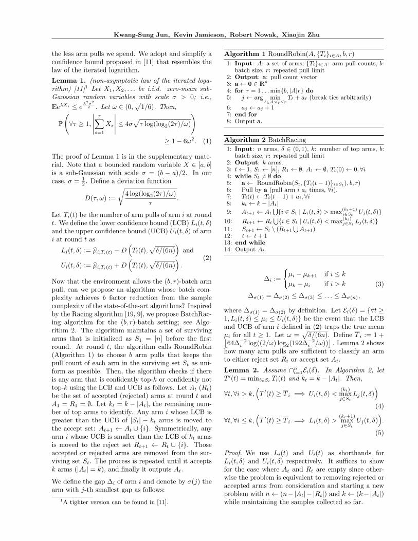
Now that the environment allows the (b, r)-batch armpull, can we propose an algorithm whose batch com-plexity achieves b factor reduction from the samplecomplexity of the state-of-the-art algorithms? Inspiredby the Racing algorithm [19, 9], we propose BatchRac-ing algorithm for the (b, r)-batch setting; see Algo-rithm 2. The algorithm maintains a set of survivingarms that is initialized as S

1

= [n] before the firstround. At round t, the algorithm calls RoundRobin(Algorithm 1) to choose b arm pulls that keeps thepull count of each arm in the surviving set St as uni-form as possible. Then, the algorithm checks if thereis any arm that is confidently top-k or confidently nottop-k using the LCB and UCB as follows. Let At (Rt)be the set of accepted (rejected) arms at round t andA

1

= R1

= ;. Let kt = k � |At|, the remaining num-ber of top arms to identify. Any arm i whose LCB isgreater than the UCB of |St| � kt arms is moved tothe accept set: At+1

At [ {i}. Symmetrically, anyarm i whose UCB is smaller than the LCB of kt armsis moved to the reject set Rt+1

Rt [ {i}. Thoseaccepted or rejected arms are removed from the sur-viving set St. The process is repeated until it acceptsk arms (|At| = k), and finally it outputs At.

We define the gap �i of arm i and denote by �(j) thearm with j-th smallest gap as follows:

1A tighter version can be found in [11].

Algorithm 1 RoundRobin(A, {Ti}i2A, b, r)

1: Input: A: a set of arms, {Ti}i2A: arm pull counts, b:batch size, r: repeated pull limit

2: Output: a: pull count vector3: a 0 2 Rn

4: for ⌧ = 1 . . .min{b, |A|r} do5: j arg min

`2A:a`

rT` + a` (break ties arbitrarily)

6: aj aj + 17: end for8: Output a.

Algorithm 2 BatchRacing1: Input: n arms, � 2 (0, 1), k: number of top arms, b:

batch size, r: repeated pull limit2: Output: k arms.3: t 1, S

1

[n], R1

;, A1

;, Ti(0) 0, 8i4: while St 6= ; do5: a RoundRobin(St, {Ti(t� 1)}i2S

t

), b, r)6: Pull by a (pull arm i ai times, 8i).7: Ti(t) Ti(t� 1) + ai, 8i8: kt k � |At|9: At+1

AtS{i 2 St | Li(t, �) > max(k

t

+1)

j2St

Uj(t, �)}10: Rt+1

RtS{i 2 St | Ui(t, �) < max(k

t

)

j2St

Lj(t, �)}11: St+1

St \ (Rt+1

SAt+1

)12: t t+ 113: end while14: Output At.

�i :=

(

µi � µk+1

if i k

µk � µi if i > k

��(1) = ��(2) ��(3) . . . ��(n),

(3)

where ��(1) = ��(2) by definition. Let Ei(�) = {8t �1, Li(t, �) µi Ui(t, �)} be the event that the LCBand UCB of arm i defined in (2) traps the true meanµi for all t � 1. Let ! =

p

�/(6n). Define T i := 1 +⌅

64��2

i log((2/!) log2

(192��2

i /!))⇧

. Lemma 2 showshow many arm pulls are su�cient to classify an armto either reject set Rt or accept set At.

Lemma 2. Assume \ni=1

Ei(�). In Algorithm 2, letT 0(t) = mini2S

t

Ti(t) and kt = k � |At|. Then,

8t, 8i > k,⇣

T 0(t) � T i =) Ui(t, �) <(k

t

)

maxj2S

t

Lj(t, �)⌘

(4)

8t, 8i k,⇣

T 0(t) � T i =) Li(t, �) >(k

t

+1)

maxj2S

t

Uj(t, �)⌘

.

(5)

Proof. We use Li(t) and Ui(t) as shorthands forLi(t, �) and Ui(t, �) respectively. It su�ces to showfor the case where At and Rt are empty since other-wise the problem is equivalent to removing rejected oraccepted arms from consideration and starting a newproblem with n (n� |At|� |Rt|) and k (k� |At|)while maintaining the samples collected so far.

Top Arm Identification in Multi-Armed Bandits with Batch Arm Pulls

To prove (4), let i > k and bk be the arm withk-th largest empirical mean at t-th round. Weprove the contrapositive. Assume the RHS is false:

Ui(t) � max(k)j2St

Lj(t). Note that using D(Ti(t),!) D(T 0(t),!)),

Ui(t) bµi,Ti

(t) +D(T 0(t),!) µi + 2D(T 0(t),!) and

Ui(t) �(k)maxj2S

t

Lj(t) = Lbk(t) � bµbk,Tbk

(t) �D(T 0(t),!),

which implies µi + 2D(T 0(t),!) � bµbk,Tbk

(t) �D(T 0(t),!). Using bµbk,Tb

k

(t) � µk � D(T 0(t),!) that

is due to Lemma 3 (see the supplementary material),

µi + 2D(T 0(t),!) � µk � 2D(T 0(t),!)

�i 4D(T 0(t),!)

= 4p

(4/T 0(t)) log(log2

(2T 0(t))/!)

T 0(t) 64��2

i log(log2

(2T 0(t))/!).

Invert this using

⌧ c log

✓

log2

2⌧

!

◆

=) ⌧ c log

✓

2

!log

2

✓

3c

!

◆◆

(6)

with c = 64��2

i to have T 0(t) 64��2

i log((2/!) log2

(192��2

i /!)). Then,T 0(t) < 1+ b64��2

i log((2/!) log2

(192��2

i /!))c = T i.This completes the proof of (4). By symmetry, onecan show (5) as well.

Theorem 1 states the batch complexity of theBatchRacing algorithm. Hereafter, all proofs can befound in the supplementary material. Note that evenif r > bb/2c, BatchRacing pulls the same arm at mostbb/2c times in a batch. Thus, our analysis hinges onthe e↵ective repeated pull limit r0 = min{r, bb/2c} in-stead of r.

Theorem 1. If b � 2, with probability at least 1 � �,Algorithm 2 outputs the top-k arms {1, . . . , k} after atmost

1

r0T �(1) +

1

b

0

@

nX

i=bb/r0c+1

T �(i)

1

A+ log n+n

b+

1

r0+ 2

= O

1

r0��2

�(1) log

n log(��2

�(1))

�

!

+

1

b

0

@

nX

i=bb/r0c+1

��2

�(i) log

n log(��2

�(i))

�

!

1

A+ log n

!

(7)

batches. In the case of b = r = 1, the al-gorithm does so after at most

Pni=1

T �(i) =

O

✓

Pni=1

��2

�(i) log

✓

n log(�

�2�(i)

)

�

◆◆

batches.

In the case of b=r=1, BatchRacing is exactly the Rac-ing algorithm, and the batch complexity is equiva-lent to the sample complexity. The sample complex-ity of Racing stated in Theorem 1 is the best knowninsofar as the exact top-k identification problem, al-though it does not match the best known lower bound⌦(Pn

i=1

��2

i ) [17]. If r � bb/2c, one can verify thatthe batch complexity (7) reduces to 1

b fraction of thesample complexity of Racing except the additive log nterm. The log n term is the price to pay for performingbatch arm pulls, which limits adaptivity. Note that thebatch complexity is at least n/b since each arm mustbe pulled at least once. Thus, unless b is large enoughto satisfy n/b⌧ log(n), the additive log(n) is negligi-ble. For simplicity, we ignore the additive log n fromthe discussion. If r < bb/2c, r plays an interestingrole. The r factor reduction is applied to the largestterm that involves ��2

�(1). The terms involving arm

�(2), . . . ,�(bb/rc) disappear. The rest of the termsenjoy b factor reduction.

The contribution of r depends on the gaps {�i}.If the smallest gap ��(1) is much smaller than

the other gaps, the term (1/r0)T �(1) becomes dom-inant, thus making r important. On the otherhand, if the gaps are all equal, one can show thatthe overall b fold reduction is achieved regardlessof r using the fact (1/r0)��2

�(1) log(n log(��2

�(1))/�) ⇡(1/b)

Pbb/r0ci=1

��2

�(i) log(n log(��2

�(i))/�). We empiri-cally verify this case with toy experiments in Section 5.

4 The Fixed Budget Setting

We now consider the problem of identifying the top-k arms with as high a probability as possible withina given number of batches B under the (b, r)-batchsetting. An algorithm must terminate after spend-ing no more than B batches and output k arms thatare believed to be the top-k. The guarantee is typi-cally made on the misidentification probability P(A⇤ 6={1, . . . , k}) where A⇤ is the output of the algorithm.However, it is often convenient to look at its batchcomplexity that can be derived from the misidentifi-cation probability. Let H

2

= maxi2[n] i��2

�(i). Bubecket al. showed that the Successive Accepts and Rejects(SAR) algorithm for the top-k identification problemunder the fixed budget setting has the sample com-plexity of O(H

2

log2 n) [5]. One might try runningSAR by supplying SAR with bB sample budget. How-ever, such a modification breaks its theoretical guar-antee. We propose BatchSAR that extends SAR toallow (b, r)-batch arm pull, and prove its performanceguarantee.

The intuition behind BatchSAR is as follows. Imag-ine the (b = n, r = 1)-batch setting where one has

Kwang-Sung Jun, Kevin Jamieson, Robert Nowak, Xiaojin Zhu

no choice but to pull every arm once at every round.There is no room for adaptivity; eliminating an armdoes not yield more arm pulls in return. Let r =min {r, db/2e} and n = db/re. Note n � 2 by defini-tion. Similarly in the general (b, r)-batch setting, oncethe surviving number of arms becomes n or less, elimi-nating an arm does not help. For example, if r < db/2eand there are n�1 surviving arms, the maximum num-ber of arm pulls one can make in a batch is r(n�1) < b,thus wasting b� r(n� 1) arm pulls.

Algorithm 3 BatchSAR1: Input: n arms, k: the target number of top arms, b:

batch size, r: repeated pull limit, B: batch budget2: Output: k arms.3: Let n = max{db/re, 2} and c

1

= b+nmin{r, db/2e}+n

4: Define ms =8>><

>>:

⇠bB�(

Pn

i=n+1db/ie)�c1n/2+

Pn

i=n+1(1/i)1

n�s+1

⇡for s n� n

⇠bB�(

Pn

i=n+1db/ie)�c1n/2+

Pn

i=n+1(1/i)1

2

⇡for s = n� n+ 1

5: t 1, S1

[n], A1

;, Ti(0) 0, 8i 2 [n]6: for s = 1, . . . , (n� n+ 1) do7: while mini2S

s

Ti(t� 1) < ms do8: a RoundRobin(Ss, {Ti(t� 1)}i2S

s

), b, r)9: Pull by a (pull arm i ai times, 8i).10: Ti(t) Ti(t� 1) + ai, 8i11: t t+ 112: end while13: Let ts = t�1, the last round in stage s, and k0 = k�

|As|, the remaining number of top arms to identify.14: if s n� n then15: Let bµi = bµi,T

i

(ts

)

and ⇢(i) be the arm with i-th largest empirical mean in Ss so that bµ⇢(1) �. . . � bµ⇢(n�s+1)

. Let b�⇢(1) = bµ⇢(1) � bµ⇢(k0+1)

andb�⇢(n�s+1)

= bµ⇢(k0)

� bµ⇢(n�s+1)

.

16: js argmaxi2{⇢(1),⇢(n�s+1)} b�i (break ties arbi-trarily).

17: Remove arm js: Ss+1

Ss \ {js}.18: if js = ⇢(1) then19: As+1

As [ {js}20: else21: As+1

As

22: end if23: (Early exit case 1) If |Ss+1

| = k � |As+1

|, thenaccept all the remaining surviving arms A⇤ As+1

[ Ss+1

and exit the for loop.24: (Early exit case 2) If |As+1

| = k, then set A⇤ As+1

and exit the for loop.25: else26: A⇤ As [

�arg k0 maxi2S

s

bµi,Ti

(ts

)

�(break ties

arbitrarily)27: end if28: end for29: Output A⇤.

Therefore, we design BatchSAR to have two phases:(i) the first n� n stages where an arm is eliminated af-ter each stage just as SAR and (ii) the last stage whereuniform sampling is performed without any elimina-tion. BatchSAR is described in Algorithm 3. The

algorithm starts with the surviving arm set S1

= [n]and performs (n�n+1) stages. In each stage s, surviv-ing arms are pulled uniformly by calling RoundRobin(Algorithm 1) until every arm’s pull count is at leastms defined in the algorithm. Then, we choose an armjs that is the safest to remove, meaning that the em-pirical gap b�i defined in the algorithm is the largest.Note js is either the empirically best arm or the worst.The arm js is then removed from the surviving set andis accepted if js is the empirically best arm. We repeatthe same until the final stage s = (n � n + 1) wherewe choose the empirical top-k0 arms and add them tothe final accept set.

We claim that the algorithm spends no more than Bbatches. Let ts be the last round in stage s. It is easy

to see that mini2Ss

Ti(ts) ms +l

bn�s+1

m

� 1 due to

the batch e↵ect, and a surviving arm’s pull count iseither mini2S

s

Ti(ts) or mini2Ss

Ti(ts) + 1. Then,

8i 2 Ss, Ti(ts) ms +

⇠

b

n� s+ 1

⇡

. (8)

We prove the claim by the fact that tn�n+1

l

1

b

⇣

P

i2Sn�n+1

Ti(tn�n+1

) +Pn�n

s=1

Tjs

(ts)⌘m

, which

we bound by B using (8) and db/ne r.

Theorem 2 states the misidentification probability ofBatchSAR. Define

H<b,r>3

=1

b

n

2+

nX

i=n+1

1

i

!

maxi=2,n+1,n+2,...,n

i��2

�(i).

(9)

Theorem 2. Let A⇤ be the output of BatchSAR.Given a batch budget B, the misidentification probabil-ity of BatchSAR under the (b, r)-batch setting satisfies

P(A⇤ 6= {1, . . . , k})

2n2 exp

�1

8

B ��

Pni=n+1

db/ie�

/b� c1

/b

H<b,r>3

!

.

One can derive the batch complexity of Batch-

SAR as O⇣

H<b,r>3

log(n) + 1

b

Pni=n+1

⌃

bi

⌥

⌘

. The

term 1

b

Pni=n+1

⌃

bi

⌥

= O(log(n) + n/b) is the priceto pay for performing the (b, r)-batch where thealgorithm might pull an arm more than neces-sary. The batch complexity is upper-bounded by

O⇣⇣

1

r + lognb

⌘

H2

log n+ log n⌘

, where the additive

log(n) is negligible unless n/b⌧ log(n).

In the extreme case of b=r=1, the term 1

b

Pni=n+1

⌃

bi

⌥

is n, which can be ignored since the batch complexityis at least of order n when b = 1. Thus, we achieveO(H

2

log2 n), which is equivalent to the sample com-plexity of SAR. If r � db/2e, H<b,r>

3

log n + log n

Top Arm Identification in Multi-Armed Bandits with Batch Arm Pulls

1

b (2 + log n)H2

log n + log n = O( 1bH2

log2(n) + log n), which achieves an overall b factor reduction fromthe sample complexity of SAR except for the addi-tive log n. In the other extreme case where b = n andr = 1, BatchSAR reduces to uniform sampling and thebatch complexity is O(��2

�(2) log n).

Practical Considerations In general, the algo-rithm finishes earlier than B batches. The reason isthat ms is defined to defend against the worst case.In practice, one might want to exhaust the budget Bto minimize the error. Let log(b||a) =

Pbi=a+1

1

i . Wepropose to replace ms with

m0s =

2

6

6

6

bB �⇣

Ps�1

s0=1

Tjs

0 (ts0)⌘

�⇣

Pn�s+1

i=n+1

d bi e⌘

� c01

�

n/2 + log(n� s+ 1||n)�

(n� s+ 1)

3

7

7

7

(10)

where c01

= b+ nr + n� s+ 1. For the last stage s =n�n+1, we sample the surviving arms until the budgetB is exhausted. One can show that m0

s � ms after us-

ing (8) to verifyPs�1

s0=1

Tjs

0 (ts0)+⇣

Pn�s+1

i=n+1

d bi e⌘

+c01

�

Pni=n+1

d bi e�

+c1

+(bB�(

Pn

i=n+1db

i

e)�c1)

(n/2)+log(n||n) log(n||n�s+

1). Thus, Theorem 2 still holds true with m0s.

5 Experiments

We verify our theoretical results with simulation ex-periments in the fixed confidence setting, then presenttwo important applications of the (b, r)-batch MABproblem. For applications, we focus on the fixed bud-get setting due to its practicality.

5.1 Toy Experiments

The batch size b and repeated pull limit r contributeto the batch complexity in an intricate way in boththe fixed confidence and budget settings. We wouldlike to verify how b and r change the batch complexityempirically and compare it to our theory. Note thatthe batch complexity shown in the analysis considersthe worst case; the number of batches suggested bythe theory is often more than what is experienced inpractice. However, if such slack is independent of band r, we can remove it by monitoring the “speedup”,see below.

We consider two bandit instances with n=100 arms:(i) Bernoulli arms with expected rewards that linearlydecrease, i.e., µi = (99�i+1)/99, and (ii) sparsely dis-tributed Bernoulli arms where the expected rewards of10 arms are 0.5 and the rest are 0.3. We call the for-mer Linear and the latter Sparse. Note we focus on thefixed confidence setting here due to space constraints;the same result can be obtained in the fixed budgetsetting. We run BatchRacing 10 times with � = 0.1,

k=10, b 2 {1, 4, 16, 64} and r 2 {1, 2, 4, 8, 16, 32}. Foreach pair (b0, r0), we compute the empirical speedup bydividing the average number of batches in (b=1,r=1)by the average number of batches in (b0, r0). Let Mb,r

be the batch complexity computed by (7). For eachpair (b0, r0), we also compute the theory-based speedupby�

Pni=1

T �(i)

�

/Mb0,r0 .

Table 1 shows the the speedup of each (b, r)-batch.Overall, the theory-based speedup matches extremelywell with the empirical speedup. This implies thatthe rather complicated contribution of b and r in thebatch complexity well explains the reality. Note thatr plays an important role in Linear; it is only afterr = b/2 that the speedup achieves b. This is because��2

�(1) = (µk � µk+1

)�2 dominates, which boosts the

batch complexity’s reliance on the factor 1/r0. On theother hand, in Sparse the gaps {�i} are uniformly 0.2,and we achieved an overall b fold speedup (almost)regardless of r as predicted in Section 3.

5.2 Application 1: Virus Replication

Experiments

Virologists are interested in identifying which genes areimportant in virus replication. For instance, Hao etal. tested 13k genes of drosophila to find which genespromote influenza virus replication [8]. The authorsperform a sequence of batch experiments using a platewith 384 microwells. Each well contains a single-geneknock-down cell strain to which the fluorescing virus isadded. They measured the fluorescence levels after anincubation period and obtained an indication of howimportant the knock-down gene is in virus replication.Since the measurements are noisy, we formulate theproblem as a top-k identification problem in MAB.Each arm is a gene, and the reward is its knock-downfluorescence level. The batch arm pull is performedwith b=384 wells where the repeated pull limit r isequal to b since one can place the same gene knock-down in multiple wells.

Dataset We simulate the microwell experiments byassuming a Gaussian distribution on each arm, wherethe mean and variance are estimated from the actualdata. Specifically, we use two measurements from eachof the n = 12, 979 2 gene knock-downs from [8]. Forthe j-th measurement of arm/gene i, xi,j , we removethe plate-specific noise by dividing it by the averagecontrol measurement from the same plate. Then, wetake the logarithm to e↵ectively make the variance ofeach fluorescence measurement similar, following [8].We also flip the sign to call it zi,j since a low fluo-rescence level implies that the knock-down gene pro-

2The original dataset contains 13,071 genes. We found92 genes whose control was measured incorrectly, so weremoved them for the evaluation.

Kwang-Sung Jun, Kevin Jamieson, Robert Nowak, Xiaojin Zhu

b rLinear Sparse

b rLinear Sparse

Theory Actual Theory Actual Theory Actual Theory Actual4 1 2.71 2.74 4.00 4.00 64 1 3.16 3.21 63.97 58.284 2 4.00 4.00 4.00 4.00 64 2 6.32 6.41 63.97 61.8816 1 3.14 3.18 16.00 15.83 64 4 12.55 12.74 63.97 63.2516 2 6.08 6.16 16.00 15.95 64 8 24.31 24.65 63.97 63.7316 4 10.84 10.96 16.00 15.99 64 16 43.37 43.83 63.97 63.8716 8 16.00 16.00 16.00 16.00 64 32 64.00 63.99 63.97 63.90

Table 1: Toy experiment result: the speedup in the number of batches in the fixed confidence setting.

motes the replication. We set the mean of arm i asµi = (zi,1 + zi,2)/2. We compute the unbiased es-

timate of the variance bVi of each gene and computethe average (1/n)

Pni=1

bVi across all arms, which is anunbiased estimate of the variance if all arms have anequal variance. In the end, we simulate measurementsfor arm i from N (µi, 0.1). We plot the arm distribu-tion in Figure 1(a), where we see that relatively fewgenes have large rewards (that facilitate virus replica-tion).

Algorithm 4 Halving1: Input: n arms, k: the target number of top arms, b:

batch size, r: repeated pull limit, B: batch budget2: Output: k arms.3: t 1, S

1

[n], Ti(0) 0, 8i4: for s = 1 to dlog

2

nk e do

5: for i = 1 toj

Bdlog2(n/k)e

kdo

6: a RoundRobin(Ss, {Ti(t� 1)}i2Ss

, b, r)7: Pull by a (pull arm i ai times, 8i).8: Ti(t) Ti(t� 1) + ai, 8i9: t t+ 110: end for11: Let Ss+1

be the set of max{d|Ss|/2e, db/re} arms inSs with the largest empirical average.

12: end for13: Output S

1+dlog2(n/k)e.

Methods We use two algorithms as the baseline:RoundRobin and Halving. RoundRobin repeatedlypull arms according to RoundRobin (Algorithm 1)with no eliminations until the batch budget runs out.Halving adapts Sequential Halving algorithm [16], atop-1 identification algorithm, to perform top-k identi-fication under the batch setting3, though it lacks theo-retical guarantee. We describe Halving in Algorithm 4.Both Halving and BatchSAR could waste the budgetif run as is due to the integer operators. Thus, in Halv-ing we randomly spread out the remaining budget overstages, and in BatchSAR we use m0

s defined in (10) inplace of ms.

Result We run the algorithms for k 2{100, 200, 400, 800} and B 2 {100, 200, 400, 800}.We run each experiment 20 times and measure falsenegative rate (FNR). FNR is the proportion of the

3 We change the number of stages from dlog2

ne todlog

2

(n/k)e following [15] and divide stages in terms ofthe number of batches rather than samples.

top-k arms that do not appear in the output of the

algorithm: |[k]\{the output of the algorithm}|k . High

FNR was pointed out by [7] as the main issue inadaptive experiments. The result is shown in Figure 1(b-e). We plot the FNR vs. batch budget B for eachk, where the error bar is the 95% confidence interval.In all experiments, BatchSAR and Halving signifi-cantly outperform RoundRobin. RoundRobin spendsthe vast majority of arm pulls on arms with smallexpected rewards and fails to distinguish the top-karms from those near top-k. BatchSAR outperformsHalving in most cases, especially when the budget islarge.

5.3 Application 2: Twitter User Tracking

We are interested in identifying the top-k users inTwitter who talk about a given topic most frequently.For example, in the study of bullying researchers areinterested in a longitudinal study on the long term ef-fects of bullying experience [21]. Such a study in Twit-ter requires first identifying the top-k (e.g., k=100)users with frequent bullying experience, then observ-ing their posts for a long time (e.g., over a year). If onehas an unlimited monitoring access to all users (e.g.,firehose in Twitter), the first stage of identifying thetop-k users would be trivial. However, researchers areoften limited by the public API that has rate limits; forinstance, user streaming API of Twitter4 allows one tofollow at most 5000 users at a time. In MAB termi-nology, each user is an arm, one batch pull is to follow5000 users at a time for a fixed time interval, and thereward is whether or not a user posted tweets abouta bullying experience. The latter is decided by a textclassifier [25]. Even though it seems that r = 1 sincewe either follow a user or not, we discuss a procedurebelow where r can be larger.

We observe that the tweet rate of users changes sig-nificantly over time of day. Figure 2 (a) shows thedaily trend. We plot the number of bullying tweetsgenerated in each 5-minute interval where the count isaccumulated over 31 days. To get around this diurnalissue, we define a pull of an arm to be following a userfor 5 minutes every hour in a day, totaling two hours.Since there exist twelve 5-minute intervals in an hour,one can follow b = 12 · 5000 = 60,000 users in a day.

4

statuses/filter API with follow parameter.

Top Arm Identification in Multi-Armed Bandits with Batch Arm Pulls

0 5000 10000−1

0123

Arm index

Expe

cted

rew

ard

B200 400 600 800

0

0.2

0.4 BatchSARHalvingRoundRobin

B200 400 600 800

0

0.2

0.4 BatchSARHalvingRoundRobin

B200 400 600 800

0

0.2

0.4 BatchSARHalvingRoundRobin

B200 400 600 800

0

0.2

0.4 BatchSARHalvingRoundRobin

(a) Arm distribution (b) k=100 (c) k = 200 (d) k=400 (e) k=800

Figure 1: Microwell experiment result. (b-e) plots the false negative rate vs. budget B.

0 5 10 15 201000

2000

3000

4000

5000

6000

Time of day

Twee

t cou

nt p

er 5

min

utes

100 102 104 10610−4

10−3

10−2

10−1

Arm index

Expe

cted

rew

ard

Algorithm GainBatchSAR 0.17 (±0.01)Halving 0.21 (±0.02)

RoundRobin 0.09 (±0.01)Oracle 0.46

(a) (b) (c)Figure 2: (a) Twitter daily pattern (b) Expected rewards of users (c) Experiment result

Note those 60,000 users need not be unique; one canfollow the same user up to 12 times, each in a di↵erent5-minute interval. Thus, r=12. Formally, we assumethat the bullying tweet rate of a user i changes everyhour of day h, but remains the same within. Let Yi,d,h,c

indicate whether or not (1 or 0) the user i generates abullying tweet at day d hour h interval c 2 [12]. Yi,d,h,c

follows a Bernoulli(pi,h) distribution, where pi,h is thetweet probability of user i during a 5-minute intervalin hour h. We define the reward of an arm i on dayd as (1/24)

P

24

h=1

Yi,d,h,c(h) where c(h) indicates whichinterval to pick at each hour h. Then, the expected re-ward µi of an arm i is the average Bernoulli probabilityover a day: µi = (1/24)

P

24

h=1

pi,h.

Dataset The dataset consists of 707,776 bullyingtweets collected over 31 days in January 2013. Thenumber of distinct users n is 522,062. We com-pute the average reward for each user at each hourand take it as the true tweet probability pi,h :=1

31

P

31

d=1

1

12

P

12

c=1

Yi,d,h,c, from which we compute theexpected reward µi as previously shown. We plot theexpected reward in Figure 2(b), where both axes arein log

10

scale. The plot nicely follows a power law.

Result We use the same methods from Section 5.2.We set k=100 and run each algorithm 10 times dueto randomness in breaking ties. We measure the gainP

i2J µi, where J is the set of k arms output by an al-gorithm. The gain measures the quality of the selectedarms by the magnitudes of their expected rewards.The result is summarized in Figure 2(c). The numberin parentheses is the 95% confidence interval, and Ora-cle is the gain on the true top-k arms (J = {1, . . . , k}),which is the best achievable. Both Halving and Batch-SAR significantly outperforms RoundRobin. Halv-

ing, though without theoretical guarantee, performsslightly better than BatchSAR. We suspect that thereason is that Halving works well in low budget situ-ation as it was in Section 5.2. A thorough empiricalcomparison is left as a future work.

6 Future Work

There are numerous opportunities for future works inthe (b, r)-batch setting. First, adapting existing pureexploration algorithms to the batch setting and ana-lyzing their batch complexity. Not only Halving pre-sented in this work without guarantee but also LUCBwould be interesting to analyze since it is known toperform best in practice [12]. Second, investigatingthe lower bound on the batch complexity. Specifically,we have observed that the contribution of the repeatedpull limit r to the batch complexity is nontrivial. Itwould be interesting to see if the same form of con-tribution happens in the lower bound as well. Finally,we would like to extend the batch setting to accommo-date di↵erent batch sizes as in [22], but for n > 2 arms([22] only pertains to n = 2) and in the pure explo-ration setting rather than the regret setting. Varyingbatch size MAB problems can arise in clinical trialsand in crowdsourcing systems where the crowd sizedynamically changes over time.

Acknowledgments

The authors are thankful to the anonymous reviewersfor their comments. This work is supported in partby NSF grant IIS-0953219 and IIS-1447449, AFOSRgrant FA9550-13-1-0138, ONR awards N00014-15-1-2620 and N00014-13-1-0129. We thank Paul Ahlquist,Michael Newton, and Linhui Hao for providing thevirus replication experiment data and their helpful dis-cussion.

Kwang-Sung Jun, Kevin Jamieson, Robert Nowak, Xiaojin Zhu

References

[1] V. Anantharam, P. Varaiya, and J. Walrand,“Asymptotically e�cient allocation rules for themultiarmed bandit problem with multiple plays-part i: I.i.d. rewards,” Automatic Control, IEEETransactions on, vol. 32, no. 11, pp. 968–976,1987.

[2] J. Audibert, S. Bubeck, and G. Lugosi, “Regret inonline combinatorial optimization,” Mathematicsof Operations Research, vol. 39, no. 1, pp. 31–45,2014.

[3] J.-Y. Audibert, S. Bubeck, and R. Munos, “Bestarm identification in multi-armed bandits,” inProceedings of the Conference on Learning The-ory (COLT), 2010.

[4] R. E. Bechhofer, “A sequential multiple-decisionprocedure for selecting the best one of several nor-mal populations with a common unknown vari-ance, and its use with various experimental de-signs,” Biometrics, vol. 14, no. 3, pp. 408–429,1958.

[5] S. Bubeck, T. Wang, and N. Viswanathan, “Mul-tiple identifications in multi-armed bandits,” inProceedings of the International Conference onMachine Learning (ICML), 2013, pp. 258–265.

[6] E. Even-dar, S. Mannor, and Y. Mansour, “Pacbounds for multi-armed bandit and markov deci-sion processes,” in Proceedings of the Conferenceon Learning Theory (COLT), 2002, pp. 255–270.

[7] L. Hao, Q. He, Z. Wang, M. Craven, M. A. New-ton, and P. a. Ahlquist, “Limited agreement ofindependent rnai screens for virus-required hostgenes owes more to false-negative than false-positive factors,” PLoS Computational Biology,vol. 9, no. 9, p. e1003235, 2013.

[8] L. Hao, A. Sakurai, T. Watanabe, E. Sorensen,C. A. Nidom, M. A. Newton, P. Ahlquist, andY. Kawaoka, “Drosophila rnai screen identifieshost genes important for influenza virus replica-tion,” Nature, vol. 454, no. 7206, pp. 890–893,2008.

[9] V. Heidrich-Meisner and C. Igel, “Hoe↵ding andbernstein races for selecting policies in evolution-ary direct policy search,” in Proceedings of theInternational Conference on Machine Learning(ICML), 2009, pp. 401–408.

[10] W. Hoe↵ding, “Probability inequalities for sumsof bounded random variables,” Journal of theAmerican Statistical Association, vol. 58, no. 301,pp. 13–30, March 1963.

[11] K. G. Jamieson, M. Malloy, R. Nowak, andS. Bubeck, “lil’ ucb : An optimal exploration algo-rithm for multi-armed bandits,” in Proceedings ofThe 27th Conference on Learning Theory, 2014,pp. 423–439.

[12] K. G. Jamieson and R. Nowak, “Best-arm identi-fication algorithms for multi-armed bandits in thefixed confidence setting,” in 48th Annual Confer-ence on Information Sciences and Systems, CISS,2014, pp. 1–6.

[13] P. Joulani, A. Gyorgy, and C. Szepesvari, “On-line learning under delayed feedback.” in Proceed-ings of the International Conference on MachineLearning (ICML), 2013, pp. 1453–1461.

[14] S. Kalyanakrishnan and P. Stone, “E�cient selec-tion of multiple bandit arms: Theory and prac-tice,” in Proceedings of the International Con-ference on Machine Learning (ICML), 2010, pp.511–518.

[15] S. Kalyanakrishnan, A. Tewari, P. Auer, andP. Stone, “PAC subset selection in stochas-tic multi-armed bandits,” in Proceedings of theInternational Conference on Machine Learning(ICML), 2012, pp. 655–662.

[16] Z. S. Karnin, T. Koren, and O. Somekh, “Almostoptimal exploration in multi-armed bandits.” inProceedings of the International Conference onMachine Learning (ICML), 2013, pp. 1238–1246.

[17] E. Kaufmann, O. Cappe, and A. Garivier,“On the complexity of best-arm identification inmulti-armed bandit models,” Journal of MachineLearning Research, vol. 17, no. 1, pp. 1–42, 2016.

[18] A. Niculescu-Mizil, “Multi-armed bandits withbetting,” in COLT’09 Workshop on On-lineLearning with Limited Feedback, 2009.

[19] A. M. Oded Maron, “Hoe↵ding races: Accelerat-ing model selection search for classification andfunction approximation,” in Advances in Neu-ral Information Processing Systems (NIPS), April1994, pp. 59–66.

[20] E. Paulson, “A sequential procedure for select-ing the population with the largest mean fromk normal populations,” Annals of MathematicalStatistics, vol. 35, no. 1, pp. 174–180, 1964.

[21] A. D. Pellegrini and J. D. Long, “A longitudinalstudy of bullying, dominance, and victimizationduring the transition from primary school throughsecondary school,” British Journal of Develop-mental Psychology, vol. 20, no. 2, pp. 259–280,2002.

Top Arm Identification in Multi-Armed Bandits with Batch Arm Pulls

[22] V. Perchet, P. Rigollet, S. Chassang, andE. Snowberg, “Batched bandit problems,” in Pro-ceedings of the Conference on Learning Theory(COLT), 2015, pp. 1456–1456.

[23] M. J. Weinberger and E. Ordentlich, “On delayedprediction of individual sequences.” IEEE Trans-actions on Information Theory, vol. 48, no. 7, pp.1959–1976, 2002.

[24] Y. Wu, A. Gyrgy, and C. Szepesvri, “On identi-fying good options under combinatorially struc-tured feedback in finite noisy environments.” inProceedings of the International Conference onMachine Learning (ICML), 2015, pp. 1283–1291.

[25] J.-M. Xu, K.-S. Jun, X. Zhu, and A. Bellmore,“Learning from bullying traces in social media,”in Proceedings of the North American Chapterof the Association for Computational Linguistics:Human Language Technologies (NAACL HLT),2012, pp. 656–666.

Kwang-Sung Jun, Kevin Jamieson, Robert Nowak, Xiaojin Zhu

Supplementary Material

A Proof of Lemma 1

Let S⌧ =P⌧

s=1

Xs. Note that the upper and lower bound around S⌧ is symmetric. Thus, it su�ces to showthat the upper bound on S⌧ fails with probability at most 3!2. Show that {eS⌧ } is sub-Martingale, applyDoob’s maximal inequality to it, then use the definition of the sub-Gaussian and Markov’s inequality to have

P✓

max⌧=1,...,m

S⌧ � x

◆

e�x

2

2m�

2 . Define

E1

=\

k�0

⇢

S2

k 2�q

2k log(log2

(2 · 2k)/!)�

E2

=\

k�1

2

k+1\

⌧=2

k

+1

⇢

S⌧ � S2

k 2�q

2k log(log2

(2 · 2k)/!)�

.

One can verify that E1

\ E2

implies the upper bound stated in the Lemma since (i) for ⌧ = 1 and 2, E1

impliesthe bound and (ii) for all ⌧ � 3 such that 2k < ⌧ 2k+1 for some k,

S⌧ S2

k + 2�q

2k log(log2

(2 · 2k)/!) 4�q

2k log(log2

(2 · 2k)/!) < 4�p

⌧ log(log2

(2⌧)/!).

The failure probability of the bound is at most P(E1

) + P(E2

), which we bound with 3!2 as follows:

P(E1

) X

k�0

e�2 log(log2(2k+1

)/!) ⇡2

6!2 < 2!2

P(E2

) X

k�1

P

0

@

2

k+1[

⌧=2

k

+1

⇢

S⌧ � S2

k � 2�q

2k log(log2

(2 · 2k)/!)�

1

A

=X

k�1

P

0

@

2

k+1[

⌧=2

k

+1

8

<

:

⌧X

i=2

k

+1

Xi � 2�q

2k log(log2

(2 · 2k)/!)

9

=

;

1

A

=X

k�1

P

0

@

2

k

[

j=1

⇢

Sj � 2�q

2k log(log2

(2 · 2k)/!)�

1

A

X

k�1

✓

!

k + 1

◆

2

= (⇡2/6� 1)!2 < !2.

B Proof of Theorem 1

Lemma 3 states that the true mean of arm i can be bounded by the empirical top-i arm.

Lemma 3. Denote by bi the index of the arm whose empirical mean is i-th largest: i.e., bµb1

� . . . � bµbn. Assumethat the empirical means of the arms are controlled by ✏: i.e., 8i, |bµi � µi| ✏. Then,

8i, µi � ✏ bµbi µi + ✏.

Proof. To show µi � ✏ bµbi, consider two cases: (i) empirically i-th largest arm is true top-i, i.e. bi i, and (ii)

is not true top-i, i.e. bi > i. Case (i) implies that µbi � µi. Then,

bµbi � µbi � ✏ � µi � ✏.

Case (ii) implies that there exists an arm ` that is true top-i, but not empirical top-i, i.e. µ` � µi and bµ` bµbi,since otherwisebi (the empirical top-i) must have been squeezed out of the empirical top-i, which is a contradiction.Then,

bµbi � bµ` � µ` � ✏ � µi � ✏.

One can show bµbi µi + ✏ by symmetry.

Top Arm Identification in Multi-Armed Bandits with Batch Arm Pulls

The key insight in proving the batch complexity of BatchRacing is that once there are only bb/rc or less survivingarms, there is no choice but to pull each arm r times at every batch, possibly wasting some arm pulls. Beforethen, the algorithm fully exploits pulling b times in a round and enjoys a full factor of b reduction.

Proof. Note a random variable X such that X 2 [0, 1] w.p. 1 is sub-Gaussian with scale � = 1/2. By Lemma 1,P(\ni=1

Ei(!)) � 1 � �. Thus, it is safe to assume that \ni=1

Ei(!); the true mean of each arm is trapped by theLCB and UCB.

Correctness We show that if an arm i is accepted (rejected) then i is (not) top-k. It su�ces to prove for roundt such that At and Rt are empty for the same reason stated in the proof of Lemma 2. An arm i being acceptedimplies that there are (n� k) arms whose true means are smaller than µi since the LCB and UCB of each armtrap its true mean. Thus, i is a top-k arm. Similarly, if an arm j is rejected then j is not top-k.

Batch Complexity Let T 0(t) = mini2St

Ti(t). When T 0(t) goes above T i for some arm i, then we know byLemma 2 that arm i is either accepted or rejected and is removed from St. We consider the worst case where anarm i is removed only after satisfying T 0(t) � T i, and the order of the removal is arm �(n),�(n � 1), . . . ,�(3),and �(2) or �(1). Any early removal of an arm and switching the order of the removal necessarily make the restof the problem easier: i.e., required number of arm pulls are reduced.

By Lemma 2, when T 0(t) reaches T i, arm �(i) is removed. If b = r = 1, the batch complexity can be triviallyobtained by summing up T i for i 2 [n]. Thus, we consider b � 2 for the rest of the proof. Let ti be the roundthat T 0(ti) just passed T �(i): i.e., T

0(ti � 1) < T i and T 0(ti) � T �(i). Note that T 0(ti) can be greater than T �(i)

due to the “batch e↵ect” where the increment of the number of samples of an arm can be greater than 1. Suchdiscrepancy can be large when b is much larger than |St

i

|. It is easy to see that T 0(ti) T i+ db/|Sti

|e�1. Then,

T�(i)(ti) T 0(ti) + 1 T �(i) +

⇠

b

|Sti

|

⇡

= T �(i) +

⇠

b

(n� i+ 1)

⇡

. (11)

Consider the round t0 ⌘ t(bb/r0c+1)

where arm �(bb/r0c+ 1) is just removed. The total number of samples usedup to t0 is

bt0 =nX

i=1

T�(i)(t0)

�

b

r0

⌫

(T 0(t0) + 1) +nX

i=bb/r0c+1

T �(i) +

⇠

b

n� i+ 1

⇡

.

At round t0 + 1, there are only bb/r0c surviving arms. The algorithm then has no choice but to pull everysurviving arm r0 times in each round until we remove the hardest two arms �(1) and �(2) during which arm�(3), . . . ,�(db/r0e) are removed as a byproduct. The extra number of batches that must be performed untiltermination is then d 1

r0 (T �(2) � T 0(t0))e. Therefore, the total number of batches is

t0 +

⇠

1

r0(T �(2) � T 0(t0))

⇡

1

r0T �(2) +

1

b

nX

i=bb/r0c+1

✓

T �(i) +

⇠

b

n� i+ 1

⇡◆

+1

r0+ 1

1

r0T �(2) +

1

b

0

@

nX

i=bb/r0c+1

T �(i)

1

A+ 1 + log n+n

b+

1

r0+ 1

= O

0

@

1

r0T �(2) +

1

b

nX

i=bb/r0c+1

T �(i) + log n

1

A .

C Proof of Theorem 2

We define an event ⇠s where every arm’s empirical mean is controlled as follows:

⇠s =

8

<

:

n

8i 2 [n],�

�

bµi,Ti

(ts

)

� µi

�

� �

�(n�s+1)

4

o

if s n� nn

8i 2 [n],�

�

bµi,Tn�n+1(tn�n+1)

� µi

�

� �

�(2)

4

o

if s = n� n+ 1.

Kwang-Sung Jun, Kevin Jamieson, Robert Nowak, Xiaojin Zhu

The proof consists of two parts. We first upper bound the probability that the empirical means are not controlled,which is P([n�n+1

s=1

⇠s). Next, we show that when the empirical means are controlled, i.e. \n�n+1

s=1

⇠s, Algorithm 3terminates with the correct top-k arms.

Upperbound the Probability P([n�n+1

s=1

⇠s) Define Z = n/2 +Pn

i=n+1

1/i. By Hoe↵ding’s bound [10], fors n� n,

P(⇠s) nX

i=1

2 exp

�2Ti(ts)�2

�(n�s+1)

16

!

2n exp

�2ms

�2

�(n�s+1)

16

!

2n exp

�1

8Z�1

bB ��

Pni=n+1

db/ie�

� c1

(n� s+ 1)��2

�(n�s+1)

!

,

and similarly P(⇠n�n+1

) 2n exp

✓

� 1

8

Z�1

bB�(P

n

i=n+1db/ie)�c1

2�

�2�(2)

◆

. By union bound, P([n�n+1

s=1

⇠s) (n � n +

1)2n exp

✓

� 1

8

Z�1

bB�(P

n

i=n+1db/ie)�c1

max

i=2,n+1,...,n i��2�(i)

◆

2n2 exp

✓

� 1

8

B�(P

n

i=n+1db/ie)/b�c1/b

H<b,r>

3

◆

.

Correctness of the first stage We show that at every stage s the algorithm makes a correct decision giventhat ⇠s is true: the selected arm js is accepted if it is top-k and not accepted if it is not top-k. We prove it byinduction. We first show that the decision at the first stage is correct. Then, assuming that the decision at theround s is correct, we show that the stage s+ 1 is also correct.

Consider the first stage. Assume that ⇠s is true. Suppose the decision on the selected arm j1

at the first stageis incorrect. There are two cases: (a) j

1

is not top-k but is accepted and (b) j1

is top-k but not accepted.

We here prove that (a) leads to a contradiction; one can show the same for (b) symmetrically. Define theempirical gap

b�⇢(i) =

(

bµ⇢(i),T⇢(i)(ts) � bµ⇢(k+1),T

⇢(k+1)(ts) if i k

bµ⇢(k),T⇢(k)(ts) � bµ⇢(i),T

⇢(i)(ts) if i > k.

Since j1

is not top-k, i.e., j1

> k, and satisfies (a), j1

has the largest empirical gap and the largest empiricalmean:

b�j1 � b�`, 8` 2 S1

. (12)

bµj1 = bµ⇢(1). (13)

Note that ��(n) is either µ1

� µk+1

or µk � µn.

Case (a1): ��(n) = µ1

� µk+1

. By (13) and Lemma 3,

µj1 +��(n)/4 � bµj1 = bµ⇢(1) � µ1

���(n)/4=) µk+1

� µj1 � µ1

���(n)/2 = (µ1

+ µk+1

)/2=) µk+1

� µ1

,

which contradicts µ1

� µk > µk+1

.

Case (a2): ��(n) = µk � µn

By (12),

bµj1 � bµ⇢(k+1)

� bµ⇢(k) � bµ⇢(n)

� µk ���(n)/4� (µn +��(n)/4) = ��(n)/2

Note that arm 1, . . . , k have the following lower bound: 8i k, bµi � µi ���(n)/4 � µk ���(n)/4. Using (13),bµj1 = bµ⇢(1) � µ

1

� ��(n)/4 � µk � ��(n)/4. Thus, there are k + 1 arms whose empirical mean is at leastµk ���(n)/4. This gives us a lower bound for the (k + 1)-th largest empirical mean: bµ⇢(k+1)

� µk ���(n)/4.Then,

bµj1 � bµ⇢(k+1)

� ��(n)/2µj1 +��(n)/4� (µk ���(n)/4) �

=) µj1 � µk,

Top Arm Identification in Multi-Armed Bandits with Batch Arm Pulls

which contradicts j1

> k.

Correctness of the s-th stage (s n� n) First, consider s = 2. After the first round, the arm j1

is removedfrom the surviving set S

2

. Let k0 = k � |A2

|, the remaining number of top arms to identify at the secondstage. The problem we are facing at the second stage is exactly the first stage with [n] \ {�(n)} as the survivingset S

1

and k replaced with k0. If the arm j1

was �(n), the event ⇠2

where the empirical mean of each arm iscontrolled by ��(n�1)

/4 implies that the decision at the end of the second stage is correct. What happens ifthe arm j

1

was not �(n)? Denote by �0(i) the arm with i-th smallest gap in S2

and define the gap accordingly:�0

�0(1)

. . . �0�0

(n�1)

. Assuming that the decision at the first stage was correct, it is easy to verify that the

largest gap �0�0

(n�1)

in S2

is no less than ��(n�1)

. Therefore, the event ⇠2

implies that the empirical means of

arms are controlled by �0�0

(n�1)

/4, which ensures that the decision at the second stage must be correct, too. In

other words, removing arm �(n) at the first stage is the worst case; removing other arms can only make the gapslarger and make the problem “easier”.

Correctness of the final stage It is easy to show that if arms are controlled by ��(2)/4 then the empiricalmeans of the top-k0 will be greater than any non-top-k0 in the surviving arms Sn�n+1

. Thus, the output k0 armsat the last stage is correct.