TITLE Hedging strategies using LIFFE listed equity...
29
1 TITLE Hedging strategies using LIFFE listed equity options Dritsakis Nikolaos, University of Macedonia Grose Christos, University of Macedonia Keywords: efficiency, options, implied volatility, hedge, portfolio Dr. Dritsakis Nikolaos Associate Professor of Econometrics Department of Applied Informatics University of Macedonia, Thessaloniki P.O. Box 1591, 54006, Greece Phone: ++30310891876 e-mail: [email protected] Mr. Grose Christos Doctoral Student Department of Applied Informatics University of Macedonia, Thessaloniki P.O. Box 1591, 54006, Greece Phone: ++30310891847 e-mail: [email protected]
-
Upload
nguyenhuong -
Category
Documents
-
view
213 -
download
0
Transcript of TITLE Hedging strategies using LIFFE listed equity...

1
TITLE
Hedging strategies using LIFFE listed equity options
Dritsakis Nikolaos, University of Macedonia
Grose Christos, University of Macedonia
Keywords: efficiency, options, implied volatility, hedge, portfolio
Dr. Dritsakis Nikolaos Associate Professor of Econometrics Department of Applied Informatics University of Macedonia, Thessaloniki P.O. Box 1591, 54006, Greece Phone: ++30310891876 e-mail: [email protected] Mr. Grose Christos Doctoral Student Department of Applied Informatics University of Macedonia, Thessaloniki P.O. Box 1591, 54006, Greece Phone: ++30310891847 e-mail: [email protected]

2
Abstract
Ex ante tests of the efficiency of the London options market explain
alternative hedging strategies to fund managers who seek to comprehend the
opportunities in the options markets and profit by potential market
inefficiencies. Over and under valued options were used to form hedge
portfolios, which were mostly positive indicating potential inefficiencies in
LIFFE. Therefore options appear to incorporate the role of an investment
strategy on their own and not only as a hedge against positions in the
underlying stocks while the Black-Scholes formula proved to be an easily
computed and implemented way to make above normal, zero risk profits. This
paper also confirms the ability of a weighted implied standard deviation to
explain future volatility more accurately than historical volatility by use of
regression analysis.
1. Introduction
The London International Financial Futures and Options Exchange
(LIFFE) was established in 1982 in the wake of the lifting of UK foreign
exchange controls. Equity options have been trading in LIFFE, in its current
form, since 1992 when it was merged with the London Traded Options Market
(LTOM). This paper contains an empirical analysis directed towards an
investigation of whether equity options trading in LIFFE is efficient.

3
This study attempts to trace potential arbitrage opportunities in the
market. If such opportunities do not exist market efficiency appears to hold.
Since the introduction of the Black-Scholes option-pricing model many papers
have attempted to test market efficiency. However, the majority of these
studies have focused on the Chicago Board of Options Exchange. Although
LIFFE is one of the major European derivate exchanges it has not been largely
investigated.
The efficiency of LIFFE is tested against the Black-Scholes formula for
the pricing of traded options. This is because it is both easy to implement and is
widely used by dealers1. The Black-Scholes model is used to identify
overvalued and undervalued option contracts on an ex post basis by using the
hedging technique suggested by Black-Scholes (Black, 1972). The weak form
of market efficiency is tested by utilising the model’s ability to identify
overvalued and undervalued option contracts, forming hedged positions and
constructing portfolios of hedges on a one month basis. Hence, the tests for
market efficiency are jointly tests for the validity of the model and its ability in
selecting the mispriced option contracts.
In this way two further aspects of market efficiency are highlighted. First,
the ability of a trading rule to distinguish profitable from unprofitable
investments. Thus, the ability of the trading rule to explain observed prices is
ascertained. The second issue is the establishment of a trading strategy based
on this rule that will ensure above normal profits relative to the risk taken. In
1 Empirical analysis of alternative option pricing models can be found in Bakshi, Can and Chen (1997).

4
order to establish this, one can perform an ex ante test (on past data) by
replicating the existing opportunities for a trader. An ex post test on such a
trading model might give us false results. The lack of all relevant information
might lead us into falsely determining that the market is efficient.
An increasing number of investment managers, realising the potential
profits that could be made by identifying market inefficiencies, are engaging in
the options market. Their aim is twofold: Establish solid hedges against
positions taken on the underlying assets but also make profits in the options
market when such opportunities arise (Korn, 1999). Hedgers might wish to
minimise risk close to zero, under ideal conditions, but they might also want to
resort to insurance to minimise future possible unfavourable outcomes (Sheedy,
1998). Fund managers engaging in active fund management could exploit
signals of market inefficiency even though transaction costs cause expected
profits to be reduced. However, according to recent studies, option strategies
are still profitable even after transaction costs are considered (Isakov, 2001).
The remainder of the paper is organised as follows. Section 2 describes
the methodology used and is followed throughout the rest of the paper. An
analogous to the implied volatility description is done for the historical
volatility to highlight differences in the two methods accuracy. In addition tests
are performed in order to emphasise the superiority of the implied variance as a
predictor of the future variance. The results of the tests for the implied and
historical variance are presented in section 3. Then the hedging strategy results
using both the implied variance and the historical volatility are outlined on a

5
monthly collective basis. Finally, a brief reference of this paper’s conclusions
and implications are discussed in section 4.
2. Volatility trading and market efficiency
2.1 The volatility trading strategy
Our analysis will attempt to test the efficiency of traded equity options in
LIFFE, by implementing a volatility trading strategy in order to exploit
potential deviations between theoretical and actual option prices. The
formulation of a trading strategy is based on the anticipation of the future
volatility of the security underlying the option. If one expects higher (lower)
future volatility this corresponds to forecasting higher (lower) option prices as
well. Hence a successful hedger will employ a buying (selling) strategy
respectively.
The first studies that examined the deviations between theoretical and
actual prices in option prices were conducted after the B-S model was
introduced on options trading on the newly established Chicago Board of
Options Exchange (CBOE). Their common result is that indeed evidence is
inconsistent with market efficiency (Black, 1972; Galai, 1977; Trippi, 1977;
Finnerty, 1978; Klemkosky, 1980). However, as Jensen (1978) indicates,
market efficiency implies that economic profits from trading are zero, where
economic profits are risk-adjusted returns net of all costs. Hence, in some of

6
these studies after trading costs are calculated profit opportunities vanish.
Phillips and Smith (1980) as well as Wilmott, Hoggard and Whalley (1994)
also address the transaction costs issue.
In more recent studies Harvey and Whaley (1992) testing the S&P 100
index option market find that, after trading costs, a trading strategy based upon
out-of-sample volatility changes does not generate economic profits while a
study by Tan and Dickinson (1992) tests the efficiency of the stock options
market of the European Options Market by use of a spreading strategy. Joo and
Dickinson (1993) on the other hand examine the efficiency of the European
Options Market developing a dynamic hedging strategy while taking into
account the bid-ask spread cost effect. Xu and Taylor (1995) test the efficiency
hypothesis in the currency options market and Cavallo and Mammola (2000)
examine the Italian index options market, but they find that no systematic profit
can be made by singling out potential mispricings.
2.2 The Merton formula
We use Merton’s formula, which adjusts the B-S model for the inclusion
of dividend payments,
})2/1()/ln({})2/1()/ln({22
tt
yRESNEet
tyRESNSC RtytCD σ
σσ
σ −−+−
+−+= −− (2.1)

7
where DC is the Merton pricing formula of the call price, y is the continuously
compounded dividend payment.
We calculate the implied standard deviation )(ISD of each option contract
by entering the current option price into the evaluation equation and using
numerical solution techniques to find which price of the standard deviation
equates the LHS and RHS of Merton’s formula. A trading strategy is formed
based on the following steps:
(a). The Implied Market Value )(IMV is calculated using the weighted
average of the implied standard deviations of its stock )(WISD in the pricing
formula.
(b). The )(IMV is compared to the actual market prices so as to form short
and long positions on the traded options.
(c). A risk-free hedge is created consisting of at least one short and long
position while the amount of each option included in the hedged position
depends on the hedge ratio. The hedge ratio is the reciprocal of the derivative
of (2.1) and is defined,
})2/1()/ln({/)(2
1
ttyRESNe
SC ytD
σσ+−+
=∂∂ − (2.2)

8
2.3 Data
The main body of the data consists of end of month data for LIFFE listed
options during the period January 1995 – December 1999 written on twenty
London Stock Exchange (LSE) listed options. The data were obtained from
LIFFE. The quoted call prices were approximately 7,200 and for each one a
corresponding fair value was calculated.
In order to achieve synchronisation of the transactions on the LSE and
LIFFE a complex and time-consuming procedure was carried out. From the list
of call and share prices we selected the call premium and share price at the
same time so as to bypass any estimation error. The share prices used are not
closing prices but transaction prices on the last trading day of the month that
coincide with the transactions made at the same time on LIFFE in the
underlying option contracts. During the 60 observation dates five stock splits
took place and the option data were modified to accommodate the changes.
The selected companies were divided into two groups of ten; one based on
the January, April, July and October cycle and the other on the February, May,
August and November cycle. Furthermore, the chosen listed shares have had
continuously traded option contracts. The above restrictions ensured the
accuracy of the ensuing results.
The risk-free interest rate was taken from the 3-month interbank deposit rate.
For the inclusion of the dividend component in the B-S formula the dividend
that the underlying stockholder is entitled to receive was used and was then

9
converted to an equivalent continuous rate. The above data were derived from
DataStream.
2.4 Volatility estimation
The dynamic strategy was implemented using historic and implied
estimates for future volatility. Historic volatility estimation is based on the
assumption that the volatility that prevailed over the recent past will continue to
hold in the future. Initially, we take a sample of returns on the stock over a
single period. These returns are then converted into continuously compounded
returns. Lastly, the standard deviation of the compounded returns is calculated.
Lets assume that we have i continuously compounded returns, where
each return is identified as tS which equals )ln(1
2
t
t
SS and t goes from 1 to i .
Alternatively if there was an ex-dividend day during the interval,
[ ]12 /)(ln ttt SDSS += where D is the dividend payment. Therefore the mean
return and variance are as follows:
iS
S ti
tΣ=
=1
(2.3)
1
/)()(
1
)(1 1
22
1
2
2
−
−=
−
−=
∑ ∑∑= ==
i
iSS
i
SSi
t
i
ttt
i
tt
σ (2.4)

10
Volatility is therefore Sσν = where S is the average stock price of all iS ’s, tS
is the weekly stock price, i is the number of observations, v is the volatility.
Following Chiras and Manaster (1978) the implied standard deviations are
weighted by the price elasticity of an option with respect to its implied standard
deviation. The formula used is:
∑
∑
=
=
∂
∂∂
∂
=N
j j
j
j
j
N
j j
j
j
jj
CC
CC
ISDWISD
1
1
σσ
σσ
(2.5)
where N is the number of option contracts on each stock on every particular
date, WISD is the weighted implied standard deviation for each stock on every
observation date, jISD is the calculated standard deviation of each recorded
option contract, jj
jj
CCσσ
∂
∂ is the price elasticity of option j relative to its implied
standard deviation.
The importance of WISDs is twofold. Firstly, WISDs are better indicators
of future volatility than historic volatility. Secondly, they render unnecessary
the collection of historical data. Nonetheless, Beckers (1981) concluded that
both historical and implied volatility provide valuable information for the user
of option models.
In order to determine the accuracy of the hypothesis that the standard
deviations deduced from option prices are a better predictor of a stock’s
volatility than the standard deviation inferred from historical data the following
regressions are tested:

11
tjPptj SHISTSFUT ,, βα += (2.6)
tjrrtj WISDSFUT ,, βα += (2.7)
tjstjsstj WISDSHISTSFUT ,,, γβα ++= (2.8)
where tjWISD , is the weighted implied standard deviation inferred from option
prices at time t , tjSHIST , is the historical standard deviation estimated using
data from time xt − to t , tjSFUT , is the standard deviation of option j from
time t to xt + , sssrrpp γβαβαβα ,,,, ,, are the estimated coefficients of the
regression parameters2.
There are 60 months (observation periods) during which our hypothesis
was tested. For each observation period data from 20 individual stocks were
used. The SHISTs and WISDs were tested against the SFUTs to determine
which predictor explains larger percentage of the future standard deviation. The
joint test of the WISDs and SHISTs tests the informational content of each
parameter, i.e. whether each one contains unique information and whether one
adds no additional information to the already known information from the other
parameter.

12
2.5 Methodology
For the calculation of the WISDs a numerical search routine is used that
solves for σ by equating the B-S model price to the observed market price.
This happens since it is impossible to solve the B-S option-pricing model for
σ . Approximately 5.6 option contracts on a monthly basis were used to
calculate the WISDs for each option. On some cases the market price of the call
is too low to allow convergence by a model price. Lastly, throughout the
sample period in only eight cases less than three standard deviation estimates
were used for the calculation of the WISDs .
The calculated WISDs are used as the volatility component in the B-S
formula in order to calculate the option model price )(IMV . Stock margin
prices are used as input in the B-S formula. The computed model price of each
option contract is then compared to the market price to identify possible short
or long positions. When the model price is lower (higher) than the market price
the option is undervalued (overvalued) and a long (short) position is taken in
the call with a corresponding short (long) position in the stock as long as their
difference is not less than ten percent. This threshold level for the difference
between calculated and effective prices was fixed at a high level (10%) in order
to account for potential inefficiencies of the model.
In order to create a risk-free hedge at least one short and one long position
are required. If for a particular stock more than one short and long position
2 For a detailed analysis for volatility estimation in option pricing see Christensen and Brabhala (1998).

13
exists the ones bearing the maximum percentage difference are chosen. The
hedge ratio is calculated so as to determine the amount of each option included
in the hedge. This follows the acknowledgement that a successful option
strategy involves not only a position in a mispriced option, but also an
appropriate hedge in the underlying stock. In this way each pair of options will
produce offsetting gains and losses for any immediate movement in the
underlying stock price.
The first step in the process is calculating the derivative of the B-S
formula adjusted for dividend payments with respect to the stock price:
Rtyt edNEdNSeC −− ∗−∗= )()( 21 (2.9)
)( 1dNeSC yt−=∂∂ (2.10)
Then the reciprocal of (2.10) is calculated:
)( 1
1
dNe
SC yt−−
=
∂∂ (2.11)
In order to identify the most profitable hedge ratio spread we maximize
the joint percentage deviation between the market and model prices using the
following:
)/()]()[( ''jijjii CCCCCC +−+− (2.12)

14
where 'iC is the fair value of an undervalued call, iC is the market value of the
undervalued call, 'jC is the fair value of the overvalued call, jC is the market
value of the overvalued call.
This rule has the effect of eliminating the low-priced, out of the money
options for which the model may not be a good predictor. The holding period
for each hedge is one-month (in the context of a five year period). The hedge
position is maintained over the one-month holding period and is closed out at
the opening stock and option transaction prices of the next trading day that is a
month later. During the holding period the hedge ratio may change which
would cause the characteristics of each hedge to change. This risk is diversified
away by selecting many hedge positions. The percent holding period returns
are aggregated across all hedges for the twenty stocks throughout the fifty-nine
holding periods. The sum of all these differences should give the total gain
from the hedging strategy.
3. Empirical results
3.1 Volatility estimation tests
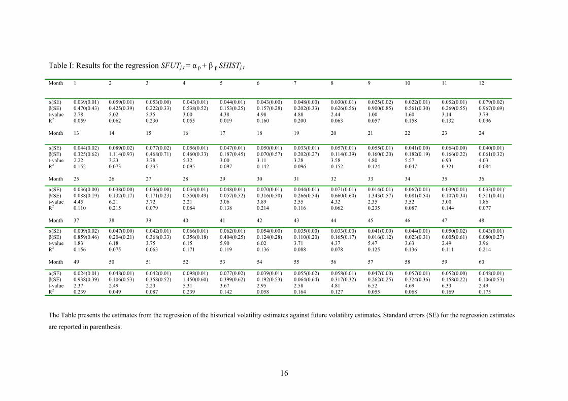
The regression estimates for equations 2.6, 2.7 and 2.8 are made using
Ordinary Least Squares method. By observing the data from Table I we note
that a very small part of the future standard deviation is explained by the
historical volatility. This feature is indicated by 2R which averages 14 percent.

15
Hence, the standard deviation of the historical volatility explained only 14
percent of the deviation of the future volatility. The 2R results do not indicate
any particular tendency towards diminishing or increasing over time.
″take in Table I″
The t values recorded are significant at the five percent significance level.
The higher the t values the lower is the probability that the sample used could
be obtained from a distribution with an actual price of β close to zero. No
negative values were recorded with mean t values approximately 4.20.
Negative t values could not be accepted because they contradict the theoretical
background.
16
Table I: Results for the regression SFUTj,t = α p + β p SHISTj,t
The Table presents the estimates from the regression of the historical volatility estimates against future volatility estimates. Standard errors (SE) for the regression estimates
are reported in parenthesis.
Month
1 2 3 4 5 6 7 8 9 10 11 12
α(SE) 0.039(0.01) 0.059(0.01) 0.053(0.00) 0.043(0.01) 0.044(0.01) 0.043(0.00) 0.048(0.00) 0.030(0.01) 0.025(0.02) 0.022(0.01) 0.052(0.01) 0.079(0.02) β(SE) 0.470(0.43) 0.425(0.39) 0.222(0.33) 0.538(0.52) 0.153(0.25) 0.157(0.28) 0.202(0.33) 0.626(0.56) 0.900(0.85) 0.561(0.30) 0.269(0.55) 0.967(0.69) t-value 2.78 5.02 5.35 3.00 4.38 4.98 4.88 2.44 1.00 1.60 3.14 3.79 R2 0.059 0.062 0.230 0.055 0.019 0.160 0.200 0.063 0.057 0.158 0.132 0.096 Month 13 14 15 16 17 18 19 20 21 22 23 24
α(SE) 0.044(0.02) 0.089(0.02) 0.077(0.02) 0.056(0.01) 0.047(0.01) 0.050(0.01) 0.033(0.01) 0.057(0.01) 0.055(0.01) 0.041(0.00) 0.064(0.00) 0.040(0.01) β(SE) 0.325(0.62) 1.114(0.93) 0.468(0.71) 0.460(0.33) 0.187(0.45) 0.070(0.57) 0.202(0.27) 0.114(0.39) 0.160(0.20) 0.182(0.19) 0.166(0.22) 0.061(0.32) t-value 2.22 3.23 3.78 5.32 3.00 3.11 3.28 3.58 4.80 5.57 6.93 4.03 R2 0.152 0.073 0.235 0.095 0.097 0.142 0.096 0.152 0.124 0.047 0.321 0.084 Month 25 26 27 28 29 30 31 32 33 34 35 36
α(SE) 0.036(0.00) 0.038(0.00) 0.036(0.00) 0.034(0.01) 0.048(0.01) 0.070(0.01) 0.044(0.01) 0.071(0.01) 0.014(0.01) 0.067(0.01) 0.039(0.01) 0.033(0.01)` β(SE) 0.088(0.19) 0.132(0.17) 0.171(0.23) 0.550(0.49) 0.057(0.52) 0.316(0.50) 0.266(0.54) 0.660(0.60) 1.343(0.57) 0.081(0.54) 0.107(0.34) 0.511(0.41) t-value 4.45 6.21 3.72 2.21 3.06 3.89 2.55 4.32 2.35 3.52 3.00 1.86 R2 0.110 0.215 0.079 0.084 0.138 0.214 0.116 0.062 0.235 0.087 0.144 0.077 Month 37 38 39 40 41 42 43 44 45 46 47 48
α(SE) 0.009(0.02) 0.047(0.00) 0.042(0.01) 0.066(0.01) 0.062(0.01) 0.054(0.00) 0.035(0.00) 0.033(0.00) 0.041(0.00) 0.044(0.01) 0.050(0.02) 0.043(0.01) β(SE) 0.859(0.46) 0.204(0.21) 0.368(0.33) 0.356(0.18) 0.404(0.25) 0.124(0.28) 0.110(0.20) 0.165(0.17) 0.016(0.12) 0.023(0.31) 0.005(0.61) 0.080(0.27) t-value 1.83 6.18 3.75 6.15 5.90 6.02 3.71 4.37 5.47 3.63 2.49 3.96 R2 0.156 0.075 0.063 0.171 0.119 0.136 0.088 0.078 0.125 0.136 0.111 0.214 Month 49 50 51 52 53 54 55 56 57 58 59 60
α(SE) 0.024(0.01) 0.048(0.01) 0.042(0.01) 0.098(0.01) 0.077(0.02) 0.039(0.01) 0.055(0.02) 0.058(0.01) 0.047(0.00) 0.057(0.01) 0.052(0.00) 0.048(0.01) β(SE) 0.938(0.39) 0.106(0.53) 0.358(0.52) 1.450(0.60) 0.399(0.62) 0.192(0.53) 0.064(0.64) 0.317(0.32) 0.262(0.25) 0.324(0.36) 0.158(0.22) 0.106(0.53) t-value 2.37 2.49 2.23 5.31 3.67 2.95 2.58 4.81 6.52 4.69 6.33 2.49 R2 0.239 0.049 0.087 0.239 0.142 0.058 0.164 0.127 0.055 0.068 0.169 0.175

17
The results for equation 2.7 (Table II) support the hypothesis that WISDs
provide better estimates of future volatility than SHISTs . 2R average value is
26 percent, almost double the SHISTs value, which can be interpreted as
WISDs having double the predictive ability of SHISTs . Nonetheless, there does
not seem to exist any particular trend on these results either, a fact which would
indicate a change in the predictive ability throughout the sample.
″take in Table II″
The majority of t values are significant at the five percent significance
level with five values bearing significance at the 0.01 level. Since t values are
still particularly high averaging 3.86 it could be stated that the null hypothesis
of β equalling zero is rejected for both regressions.
The coefficient standard errors appear to be higher for s'β rather than for
the constant in both regressions. From the results in table I the calculated mean
value for sa' is 0.0097 and for s'β 0.38. The mean constant value is 0.0234,
while the mean β is 0.0935.
In Table III the results from the joint regression are shown. The figures
partially support the conclusions drawn by the previous regressions. The t
values are significantly higher for the WISDs rather than for the SHISTs even
though in both negative values appear. The WISDs mean t value is 0.93
whereas the SHISTs mean value is 0.45. This notable difference in their
predictive power is not fully supported by the 2R results that are slightly higher
than regression (2.7) 2R results. The mean of 0.32 (compared to 0.26 in
regression 2.7) signals the existence of at least some informational content in

18
SHISTs that is not fully contained in the WISDs . In spite of this result WISDs
still appear to be better predictors of future standard deviations and to contain
the multitude of information required to make an accurate prediction of SFUTs .
These findings are consistent with Canina and Figlewski (1993) that also assert
that implied volatilities are better predictors of future volatility than those
obtained using historic data.
″take in Table III″

19
Table II: Results for the regression SFUTj,t = α r + β r WISDj,t
The estimates from the regression of implied volatility estimates against future volatility estimates are presented in this Table. Standard errors (SE) for the regression
estimates are reported in parenthesis.
Month 1 2 3 4 5 6 7 8 9 10 11 12
α(SE) 0.052(0.01) 0.062(0.01) 0.036(0.01) 0.076(0.01) 0.034(0.01) 0.055(0.01) 0.038(0.01) 0.052(0.01) 0.049(0.01) 0.062(0.01) 0.055(0.02) 0.029(0.02) β(SE) 0.003(0.05) 0.050(0.05) 0.037(0.04) 0.067(0.03) 0.017(0.05) 0.052(0.04) 0.015(0.03) 0.028(0.04) 0.004(0.07) 0.053(0.04) 0.015(0.07) 0.083(0.07) t-value 2.95 3.81 2.92 6.74 2.03 4.06 3.55 4.08 2.05 3.99 2.29 1.32 R2 0.125 0.087 0.242 0.148 0.215 0.076 0.187 0.129 0.254 0.198 0.238 0.161 Month 13 14 15 16 17 18 19 20 21 22 23 24
α(SE) 0.060(0.03) 0.041(0.05) 0.025(0.04) 0.047(0.03) 0.083(0.04) 0.071(0.04) 0.029(0.02) 0.101(0.03) 0.054(0.03) 0.018(0.02) 0.047(0.02) 0.001(0.02) β(SE) 0.025(0.15) 0.063(0.20) 0.166(0.19) 0.016(0.14) 0.123(0.16) 0.528(0.19) 0.308(0.12) 0.211(0.16) 0.030(0.12) 0.122(0.12) 0.043(0.08) 0.162(0.11) t-value 1.61 0.80 0.83 1.38 2.08 2.73 2.49 2.68 1.76 1.01 2.28 1.36 R2 0.208 0.224 0.187 0.149 0.182 0.292 0.256 0.183 0.263 0.175 0.149 0.203 Month 25 26 27 28 29 30 31 32 33 34 35 36
α(SE) 0.026(0.01) 0.030(0.01) 0.034(0.01) 0.014(0.02) 0.063(0.02) 0.046(0.03) 0.022(0.02) 0.073(0.02) 0.030(0.03) 0.051(0.01) 0.028(0.02) 0.034(0.02) β(SE) 0.057(0.06) 0.057(0.08) 0.041(0.07) 0.277(0.12) 0.074(0.09) 0.056(0.14) 0.126(0.110 0.082(0.11) 0.118(0.13) 0.061(0.07) 0.063(0.09) 0.083(0.10) t-value 1.74 1.60 1.95 2.30 2.96 1.41 1.05 2.79 0.99 2.84 1.33 1.39 R2 0.244 0.226 0.195 0.227 0.135 0.208 0.258 0.229 0.243 0.235 0.226 0.236 Month 37 38 39 40 41 42 43 44 45 46 47 48
α(SE) 0.028(0.02) 0.043(0.01) 0.048(0.02) 0.047(0.01) 0.033(0.01) 0.058(0.00) 0.018(0.01) 0.026(0.01) 0.035(0.01) 0.048(0.01) 0.048(0.02) 0.038(0.01) β(SE) 0.094(0.02) 0.012(0.05) 0.025(0.09) 0.001(0.08) 0.065(0.07) 0.004(0.00) 0.100(0.08) 0.068(0.07) 0.031(0.06) 0.025(0.07) 0.008(0.11) 0.042(0.09) t-value 1.42 3.39 2.23 2.53 2.04 3.64 1.15 1.78 2.57 3.21 2.03 1.99 R2 0.252 0.222 0.223 0.188 0.238 0.218 0.268 0.248 0.213 0.206 0.200 0.211 Month 49 50 51 52 53 54 55 56 57 58 59 60
α(SE) 0.061(0.03) 0.014(0.03) 0.057(0.04) 0.021(0.03) 0.002(0.04) 0.024(0.03) 0.071(0.03) 0.012(0.03) 0.019(0.02) 0.015(0.02) 0.050(0.02) 0.014(0.03) β(SE) 0.004(0.12) 0.223(0.12) 0.008(0.13) 0.121(0.12) 0.209(0.13) 0.065(0.10) 0.061(0.12) 0.121(0.12) 0.071(0.06) 0.109(0.09) 0.012(0.08) 0.223(0.12) t-value 1.67 1.77 1.40 0.94 1.56 0.81 1.90 0.99 1.03 1.20 1.95 1.77 R2 0.174 0.148 0.263 0.246 0.119 0.220 0.212 0.252 0.256 0.274 0.201 0.148

20
Table III: Results for the regression SFUTj,t = αs + βs SHISTj,t +γs WISD
The Table reports the estimates from the joint regression tests of implied volatility estimates and historical volatility estimates against future
volatility estimates. t-values are reported separately for each regressor.
Month 1 2 3 4 5 6 7 8 9 10 11 12
β 0.024 -0.040 0.036 -0.061 0.017 -0.049 0.015 -0.039 -0.027 0.074 0.014 0.105 γ 0.470 -0.365 -0.207 0.391 -0.153 0.063 -0.199 0.746 1.009 0.658 0.266 -1.137 t-value(β) 0.01 -0.74 0.84 -1057 0.31 -1.07 0.40 -0.97 -0.32 -1.62 0.18 1.41 t-value(γ) 1.03 -0.90 -0.607 0.76 0.58 0.21 -0.58 1.28 1.07 2.21 0.46 -1.65 R2 0.059 0.092 0.062 0.176 0.325 0.279 0.113 0.332 0.263 0.271 0.314 0.191 Month 13 14 15 16 17 18 19 20 21 22 23 24
β -0.008 0.008 0.167 0.030 -0.125 0.549 0.326 -0.224 -0.028 0.132 0.033 0.212 γ 0.318 -1.104 -0.475 -0.465 0.194 -0.305 -0.077 -0.189 -0.160 0.198 -0.152 0.235 t-value(β) -0.05 0.04 0.83 -0.22 -0.74 2.74 2.30 -1.30 -0.21 1.09 0.37 1.46 t-value(γ) 0.48 -1.12 -0.65 -1.35 0.42 -0.61 -0.28 -0.48 -0.76 1.03 -0.66 0.63 R2 0.315 0.373 0.261 0.297 0.240 0.308 0.260 0.295 0.336 0.209 0.338 0.214 Month 25 26 27 28 29 30 31 32 33 34 35 36
β 0.069 0.071 0.059 0.280 -0.085 0.052 0.126 -0.087 0.073 0.064 0.062 0.081 γ 0.137 0.155 0.216 0.572 -0.202 -0.308 0.266 -0.680 1.281 0.063 0.103 0.504 t-value(β) 1.01 0.80 0.74 2.37 -0.86 0.36 1.03 -0.78 0.60 0.78 0.67 0.80 t-value(γ) 0.68 0.89 0.88 1.30 -0.36 -0.59 0.48 -1.11 2.17 0.10 0.29 1.20 R2 0.368 0.285 0.259 0.297 0.242 0.328 0.371 0.295 0.251 0.336 0.331 0.211 Month 37 38 39 40 41 42 43 44 45 46 47 48
β 0.063 -0.016 -0.152 -0.041 0.041 -0.245 0.099 0.076 0.033 -0.025 0.018 0.044 γ 0.791 -0.208 0.368 -0.381 -0.371 0.081 0.104 0.182 -0.008 0.006 -0.006 0.091 t-value(β) 0.67 -0.27 -0.02 -0.49 0.53 -0.45 1.11 1.06 0.46 -0.31 0.07 0.47 t-value(γ) 1.62 -0.94 1.03 -1.94 -1.36 0.26 0.51 1.06 -0.05 0.02 -0.09 0.32 R2 0.178 0.351 0.363 0.182 0.233 0.322 0.383 0.107 0.313 0.306 0.300 0.317 Month 49 50 51 52 53 54 55 56 57 58 59 60
β -0.006 0.224 -0.005 0.059 0.201 0.092 -0.061 0.148 0.062 0.126 -0.011 0.224 γ 0.938 0.118 0.357 -1.370 -0.299 0.368 -0.002 -0.394 -0.228 0.402 -0.158 0.118 t-value(β) -0.05 1.72 -0.04 0.48 1.46 0.79 -0.45 1.22 0.89 1.37 -0.12 1.72 t-value(γ) 2.31 0.23 0.66 -2.14 -0.49 0.62 -0.03 -1.19 -0.88 -1.11 -0.69 0.23 R2 0.239 0.151 0.225 0.249 0.331 0.343 0.312 0.126 0.397 0.237 0.328 0.251

21
3.2 The hedging strategy results
After establishing the potential short and long positions hedges are
formed. There are 59 holding periods one less than the actual observation
period since each hedge is held for one month. Hedge positions were taken for
all months averaging 6.35 analogous positions every holding period. During
each of periods 3, 8 and 57 one hedge was held. Moreover, for periods 2, 7 and
51 two hedges were selected. For the rest of the holding periods more than
three hedges were selected. The maximum held positions were in period 27
when 11 pairs of short and long positions were assumed.
″take in Table IV″
During the first and last part of the sample period the number of option
contracts was smaller and profits through hedging relatively low. However, in
the middle of the examination period some significant profit opportunities
arose with profits from hedging reaching the 20-25 percent margin. This
phenomenon might be due to higher volatility during that period.
Among the 59 holding periods in six cases the hedges resulted in losses
that did not exceed the six percent boundary. Nevertheless, in the majority of
cases the observed inefficiencies in the options market resulted in profits being
made. The average profit for a trader during the holding period would have
been approximately 6.29 percent. The highest overall profit made on one
month’s hedge positions was 33.48 percent on the 4th month. On the contrary,

22
the highest overall loss made on a single month’s hedge was 5.74 percent on
the 58th month.
In addition of the 375 hedges 312 were profitable which constitutes 83
percent of the total number of hedges. The gain from the short and long
positions was 122 and minus 18 of the anticipated returns respectively.
Furthermore, 89 percent of the constructed portfolios were profitable, a
fact that verifies the correctness of the followed strategy. 37 out of the 71
options selected had opening prices that were considered favourable. Both the
favourable and unfavourable options categories indicated weekly profits of
about 10 percent. Results were modified accordingly to accommodate for the
presence of transaction costs. Commission varies depending on whether the
strategy is executed by a trader or an institutional investor (Nisbet, 1992). It is
assumed that if the simulated strategies were implemented by a professional
arbitrageur the tariffs would sum up to a 0.5 percent increase to the cost of the
formation of the hedge position.
A similar strategy was followed using the historical volatility for
underlying stocks using weekly return data for the period January 1990 –
December 1994. By examining the effects using historical volatility rather than
implied volatility it was attempted to identify discrepancies in our results. The
use of the historical volatility altered significantly our results without
nonetheless enabling us to identify whether it undervalued or overvalued option

23
contracts. Hence no definite conclusions can be made as to the nature that
historical volatility affects our results.
The results of the monthly hedge returns show that the overall profits
made by using the monthly hedges were 8.22 percent. During hedge periods 7,
16, 29 and 45 only one hedge was selected while the maximum number of
hedges was 16 in periods 3 and 52. Furthermore, 92 percent of the formed
hedges were profitable while only three monthly portfolios were negative. Out
of the total number of 395 hedges 323 were profitable while only one negative
hedge exceeded the 10 percent margin. The other three negative monthly
portfolios were minus 3.32, 4.89 and 1.03 percent respectively.
The maximum percentage gain from a monthly portfolio was 26.09 on the
31st holding period. In addition, the gain on the short positions is 141 percent of
the anticipated returns while the loss on the long positions was 9 percent of the
anticipated returns. Lastly, it should be emphasised that the pattern of higher
returns in the tails of the returns distribution that was seen using the implied
volatility is not observable in the historical volatility returns.

24
Table IV: Hedging strategy results using different volatility estimates
The hedging strategy results using WISDs and historical volatility estimates are presented above. The number of hedge positions formed during
each holding period are also reported.
Holding period 1 2 3 4 5 6 7 8 9 10 11 12
Return 11.06% -5.54% 7.25% 33.48% -4.11% 22.66% 3.85% 2.21% 1.53% 10.93% 14.57% 5.45% Number of Hedges 7 2 1 9 6 7 2 1 10 9 8 6 Return using Hist. volatility 6.54% 3.39% 12.21% 24.05% 4.35% -3.32% 7.59% 8.12% 2.25% 10.24% 9.95% -1.03% Number of Hedges 5 3 16 7 9 8 1 5 4 9 8 12 Holding period 13 14 15 16 17 18 19 20 21 22 23 24
Return -5.63% 10.59% 11.26% 43.21% 19.68% 11.03% 0.24% 17.44% 7.20% 42.58% 34.48% -4.60% Number of Hedges 5 10 9 8 9 4 6 9 3 8 5 7 Return using Hist. volatility 3.25% 9.55% 15.32% 17.21% 12.08% -4.89% 5.11% 9.92% 7.29% 18.95% 17.60% 6.69% Number of Hedges 6 9 5 1 6 4 8 9 4 6 8 9 Holding period 25 26 27 28 29 30 31 32 33 34 35 36
Return 30.27% 11.03% 2.27% 23.21% 11.20% 2.33% 8.86% 0.02% 7.73% 10.60% 27.31% 7.12% Number of Hedges 8 6 11 4 6 3 5 7 6 4 8 5 Return using Hist. volatility 7.21% 11.57% 9.54% 6.73% 3.54% 14.88% 26.09% 6.57% 5.11% 3.03% -10.01% 7.28% Number of Hedges 6 7 3 8 1 4 8 6 11 9 4 6 Holding period 37 38 39 40 41 42 43 44 45 46 47 48
Return 13.65% 3.16% -1.13% 11.85% 15.37% 23.60% 25.87% 8.88% 9.69% 5.65% 9.17% 23.30% Number of Hedges 9 4 9 8 10 5 3 8 8 7 9 6 Return using Hist. volatility 10.24% 4.45% 2.32% 1.17% 15.24% 8.64% 11.72% 10.05% 4.58% 7.11% 9.36% 14.68% Number of Hedges 7 10 6 8 7 4 6 5 1 4 9 7 Holding period 49 50 51 52 53 54 55 56 57 58 59
Return 2.47% 42.37% 12.84% 13.59% 6.17% 6.28% 9.33% 14.55% 0.47% -5.74% 2.00% Number of Hedges 4 8 2 8 9 6 8 7 1 9 3 Return using Hist. volatility 4.09% 16.74% 2.25% 11.08% 4.57% 8.99% 11.64% 8.57% 3.26% 12.89% 7.50% Number of Hedges 11 14 3 16 5 8 9 4 6 3 7

25
4. Conclusions
This paper has examined the ability of the Black-Scholes option pricing
formula adjusted for dividend payments to identify mispricing in the options
market for option contracts traded in the London Financial Futures and Options
Exchange. The model proved successful in identifying over and under valued
call options on an ex-post basis. Towards this goal a weighted implied standard
deviation is calculated for each underlying stock for the most accurate
calculation of each stock’s standard deviation.
Regression results proved that the implied standard deviation provides
superior to historical volatility estimates. These results suggested that only
small part of the future volatility was explained by the calculated standard
deviation based on past data. On the contrary, improved estimates of the future
volatility are obtained when the implied standard deviation was used.
Furthermore, the model displayed the previously observed pricing bias by
undervaluing, relative to the market price, out-of-the-money call options and
pricing fairly at and in-the-money call options.
The results of ex-ante performance tests did not support option market
efficiency. Therefore, a trading strategy in the options market would offer
above normal profits for an investor even after transaction costs were
considered. This outcome contradicting the majority of the recent literature in
derivatives exchanges could be attributed to equity options’ thin trading that
causes potential mispricings in the market.

26
In order to determine this result a hedging strategy was followed whereby
above a specified level undervalued option contracts were held as long
positions whereas overvalued option contracts were chosen as short positions.
Monthly hedge returns were mostly positive while the average profit from
trading in the options market during the observation period would have been
6.29 percent. Similar hedge positions were formed based on historical volatility
results. The average portfolio returns were 8.22 percent. However, the lack of
any particular pattern in the observed results prevented us from determining the
nature of influence that the historical volatility had in our results.
The implications of these results are twofold. First, the use of the Black-
Scholes formula is a practical and easy way to identify mispriced call options
that can provide above normal zero risk profits. Consequently, the options
market cannot only be used as a hedge against positions in the underlying
stocks market but also as an investment strategy itself. Secondly, the
transaction costs effect should always be considered as it causes expected
profits to be reduced, even though they do not vanish completely, and in the
context of how often positions should be revised.
References
Bakshi, G., Can, C., Chen, Z., 1997. Empirical Performance of Alternative
Option Pricing Models. Journal of Finance 52 (5).

27
Black, F., Scholes, M., 1972. The Valuation of Option Contracts and a Test of
Market Efficiency. Journal of Finance 27(2), 399-417.
Canina, L., Figlewski, S., 1993. The Information Content of Implied Volatility.
The Review of Financial Studies 6(3) 659-681.
Cavallo, L., Mammola, P., 2000. Empirical tests of efficiency of the Italian
index options market. Journal of Empirical Finance 7, 173-193.
Chiras, D., Manaster, S., 1978. The Information Content of Option Prices and a
Test of Market Efficiency. Journal of Financial Economics 6(2-3), 213-234.
Christensen, B., Prabhala, N., 1998. The Relation Between Implied and
Realized Volatility. Journal of Financial Economics 50(2), 125-150.
Finnerty, J., 1978. The Chicago Board Options Exchange and Market
Efficiency. Journal of Financial and Quantitative Analysis 13.
Galai, D., 1977. Tests of Market Efficiency of the Chicago Board Options
Exchange. Journal of Business 50(2), 167-197.
Harvey, C., Whaley, R., 1992. Market Volatility Prediction and the Efficiency
of the S&P 100 Index Option Market. Journal of Financial Economics 31
Isakov, D., Morard, B., 2001. Improving Portfolio Performance with Option
Strategies: Evidence from Switzerland. European Financial Management 7(1),
73-91.
Jensen, M. C., 1978. Some Anomalous Evidence Regarding Market Efficiency.
Journal of Financial Economics 6(2-3), 95-101.
Joo, T.H., Dickinson, J.P., 1993. A Test of the efficiency of the European
Options exchange. Applied Financial Economics 3.

28
Klemkosky, R., Resnick, B., 1980. An Ex Ante Analysis of Put-Call Parity.
Journal of Financial Economics 8(4), 363-378.
Korn, R., Trautmann, S., 1999. Optimal Control of Option Portfolios and
Applications. OR Spectrum 21.
Merton, R., 1976. Option Pricing when the Underlying Stock Returns are
Discontinuous. Journal of Financial Economics 3(1-2), 125-144.
Nisbet, M., 1992. Put-Call Parity Theory and an Empirical Test of the
Efficiency of the London Traded Options Market. Journal of Banking and
Finance 16, 381-403.
Phillips, S. M., Smith, C.W., 1980. Trading Costs for Listed Options: The
Implications for Market Efficiency. Journal of Financial Economics 8(2), 179-
201.
Sheedy, E., Trevor, R., 1998. Evaluating the Risk of Portfolios With Options.
Centre for Studies in Money, Banking and Finance, Macquarie University,
Working Paper.
Tan, H.J., Dickinson, J.P., 1992. Tests of Options Market Efficiency: A study
of the European Options Exchange. The Review of Futures Market 9, 552-570.
Trippi, R., 1977. A Test of Option Market Efficiency using a Random-Walk
Valuation Model. Journal of Economics and Business 29, 93-98.
Verbeek, M., 2000. A Guide to Modern Econometrics. John Wiley & Sons.
Wilmott, P., Hoggard, T., Whalley, A., 1994. Hedging Option Portfolios in the
Presence of Transaction Costs. Advances in Futures and Options Research 7.

29
Xu, X., Taylor, S.J., 1995. Conditional volatility and the informational
efficiency of the PHLX currency options market. Journal of Banking and
Finance 19(5), 803-821.


![WEP - NYSE Liffe US - Client Spec v1.7[1]](https://static.fdocuments.net/doc/165x107/577d376e1a28ab3a6b95abe2/wep-nyse-liffe-us-client-spec-v171.jpg)