NBER WORKING PAPER SERIES

TIPPING AND THE DYNAMICS OF SEGREGATION

David CardAlexandre MasJesse Rothstein

Working Paper 13052http://www.nber.org/papers/w13052

NATIONAL BUREAU OF ECONOMIC RESEARCH1050 Massachusetts Avenue

Cambridge, MA 02138April 2007

We are grateful to Edward Glaeser and three anonymous referees for their insightful comments andto Ted Miguel, Joshua Angrist, Jack Porter, Bo Honoré, Mark Watson, Jose Scheinkman, and RolandBenabou for helpful discussions. David Walton, Brad Howells, and Andrew Roland provided outstandingresearch assistance. We also thank Gregg Carter and Bill Collins for the data used to construct anindex of riot severity and Albert Saiz and Susan Wachter for data on land use patterns. This researchwas funded in part by the Center for Labor Economics and the Fisher Center for Real Estate at UCBerkeley, and by the Industrial Relations Section and Center for Economic Policy Studies at PrincetonUniversity. The views expressed herein are those of the author(s) and do not necessarily reflect theviews of the National Bureau of Economic Research.

© 2007 by David Card, Alexandre Mas, and Jesse Rothstein. All rights reserved. Short sections oftext, not to exceed two paragraphs, may be quoted without explicit permission provided that full credit,including © notice, is given to the source.

Tipping and the Dynamics of SegregationDavid Card, Alexandre Mas, and Jesse RothsteinNBER Working Paper No. 13052April 2007JEL No. J15,R21,R31

ABSTRACT

In a classic paper, Schelling (1971) showed that extreme segregation can arise from social interactionsin white preferences: once the minority share in a neighborhood exceeds a critical "tipping point,"all the whites leave. We use regression discontinuity methods and Census tract data from 1970 through2000 to test for discontinuities in the dynamics of neighborhood racial composition. White populationflows exhibit tipping-like behavior in most cities, with a distribution of tipping points ranging from5% to 20% minority share. The estimated discontinuities are robust to controls for a wide varietyof neighborhood characteristics, and are as strong in the suburbs as in tracts close to high-minorityneighborhoods, ruling out the main alternative explanations for apparent tipping behavior. In contrastto white population flows, there is no systematic evidence that rents or housing prices exhibit non-linearitiesaround the tipping point. Finally, we relate the location of the estimated tipping points in differentcities to measures of the racial attitudes of whites, and find that cities with more tolerant whites havehigher tipping points.

David CardDepartment of Economics549 Evans Hall, #3880UC BerkeleyBerkeley, CA 94720-3880and NBERcard@econ.berkeley.edu

Alexandre MasIndustrial relations SectionPrinceton UniversityFirestone LibraryPrinceton NJ 08544and NBERamas@haas.berkeley.edu

Jesse RothsteinIndustrial RelationsFirestone LibraryPrinceton UniversityPrinceton, NJ 08544and NBERjrothst@princeton.edu

Social interaction models have been used to explain segregation (Schelling, 1971, 1978;

Becker and Murphy, 2000), collective action (Granovetter, 1978), persistent unemployment

(Cooper and John, 1988), and crime (Glaeser, Sacerdote and Scheinkman, 1996). The key

feature of these models is that preferences depend on other agents� choices, potentially leading to

multiple equilibria and tipping (Brock and Durlauf, 2001b; Glaeser and Scheinkman, 2003).

Researchers have attempted to identify preference spillovers by estimating the effect of peer

characteristics on individual decisions (e.g. Case and Katz, 1991; Evans, Oates and Schwab,

1992; Kling, Ludwig and Katz, 2005)1; and by testing for excess dispersion in choices across

social groups (Glaeser, Sacerdote, and Scheinkman, 1996; Graham 2005). To date, however,

there is no direct evidence of the tipping behavior predicted by many social interaction models.

In this paper we use regression discontinuity methods (Angrist and Lavy, 1999; Hahn,

Todd and van de Klaauw, 2001) to test for race-based tipping in neighborhoods. To illustrate

our approach, Figure 1 plots mean percentage changes in the white population of Chicago

Census tracts from 1970 to 1980 against the minority share in 1970.2 The figure also shows

predictions from a local linear regression model, estimated with a break at a 5% minority share �

the level identified by two alternative procedures as the most likely potential tipping point. The

graph shows clear evidence of tipping, with white population gains to the left of the tipping point

and substantial outflows just to the right. We find similar (though less extreme) patterns for a

broad sample of U.S. cities in each of the past three decades.

We begin the paper by outlining a simple model of a local housing market in which

whites� willingness to pay for homes depends on the neighborhood minority share. Under

1 See Manski (1993) for a discussion of the difficulties in testing for interaction effects, and Glaeser and Scheinkman (2003) for a review of many existing studies. 2 We express the change in white population as a fraction of the total tract population in 1970. Minorities are defined as nonwhites and white Hispanics.

-2-

certain assumptions, shifts in the relative demand of whites and minorities will lead to smooth

changes in the minority share of the neighborhood as long as the minority share remains below a

critical threshold. Beyond this tipping point all the white households will leave. The location of

the tipping point is determined in part by the strength of white preferences for minority contact,

and is higher when whites are more tolerant of minority neighbors.

We then set out to test for tipping behavior using decadal changes in neighborhood

racial/ethnic composition. A major obstacle is that the location of the tipping point is unknown.

We use two approaches to identify city-specific potential tipping points. First, drawing from the

literature on structural breaks, we select the point that yields the best fitting model for tract-level

white population changes. Second, building on the pattern in Figure 1, we fit a flexible model

for tract-level changes in white population shares in each city, and find the minority share with a

predicted change equal to the city-wide average change. The methods yield very similar tipping

points for most cities. The estimated tipping points for a given city are also highly correlated

across the three decades in our sample.

As suggested by the pattern in Figure 1, we find large, significant discontinuities in the

white population growth rate at the identified tipping points. These are robust to the inclusion of

flexible controls for other neighborhood characteristics, including poverty, unemployment, and

housing attributes. Similar tipping patterns are present in larger and smaller cities in all regions

of the country, and in both suburban and central city neighborhoods.

Neither rents nor housing prices exhibit sharp discontinuities at the tipping point.3

Nevertheless, tipping has an important effect on the quantity of new housing units, particularly in

3 In an early study, Laurenti (1960) pointed out that there is little theoretical or empirical support for the widespread belief that home values necessarily fall when neighborhoods undergo racial transition.

-3-

tracts with remaining open land where new construction is still possible. The rates of population

growth and new construction in these tracts falls markedly once a tract reaches the tipping point.

We conclude that tipping is a general feature of American cities that has persisted into

the 1990s. This contrasts with the conclusions of an earlier study using the same data (Easterly,

2005), which looked for but did not find evidence of the discontinuous neighborhood change

predicted by tipping models. Easterly assumed that the tipping point would be the same in all

cities. Our analysis indicates that this assumption is too restrictive. Failure to allow for

differences across cities in the location of the tipping point smooths out the discontinuities we

identify, masking important tipping effects.

We conclude by examining the determinants of the location of the tipping point in

different cities. Consistent with earlier work by Cutler, Glaeser and Vigdor (1999) on

preferences and segregation, we find that tipping points are higher in cities with more tolerant

whites, underscoring the role of white preferences in tipping and the dynamics of segregation.

Tipping points are also related with racial composition, racial income differences, density, crime

rates, and measures of past racial tension, all in the expected directions. They rose slightly over

the twenty years that we study, but this is more than explained by demographic changes.

II. Theoretical Framework

a. A Model of Tipping

We present a simple partial equilibrium model of neighborhood composition that treats

local housing demand functions as primitive.4 Consider a neighborhood with a homogenous

4 The literature contains many models of neighborhood choice that yield tipping behavior, including Schelling (1971,

-4-

housing stock of measure one and two groups of potential buyers: whites (w) and minorities (m).

Let bg(ng, m) (g∈{w, m}) denote the inverse demand (or bid-rent) functions of the two groups

for homes in the neighborhood when it has minority share m, so that there are ng families from

group g who are willing to pay at least bg(ng, m) to live there. By construction, the derivatives

∂bw/∂nw and ∂bm/∂nm are (weakly) negative. The derivatives ∂bw/∂m and ∂bw/∂m represent

social interaction effects on the bid-rent functions. We assume that for minority shares beyond

some threshold (say m=10%), ∂bw(nw, m)/∂m<0.5

At an integrated equilibrium with minority share m ∈ (0, 1), the mth highest minority

bidder has the same willingness to pay as the (1-m)th highest white bidder. That is,

(1) bm(m, m) = bw(1−m, m).6

The derivative of the white bid function bw(1−m, m) with respect to the neighborhood minority

share is −∂bw/∂nw + ∂bw/∂m. The first term in this expression is positive. If the social

interaction effect ∂bw/∂m is small at m=0 but becomes more negative as m rises, bw(1−m, m) will

have the shape illustrated in Figure 2 � positively sloped at m=0, but eventually downward-

sloping. We assume for illustrative purposes that bm(m,m) is downward-sloping and linear.7

In the neighborhood illustrated in Figure 2, there are three equilibria, one all-minority

and two mixed. Point A is a locally stable mixed equilibrium. Just to the right of this point, the

marginal white family has a higher willingness to pay than the marginal minority family, and

1978), Miyao (1979), and Bond and Coulson (1989). Ours is derived from Becker and Murphy (2000). 5 Survey evidence suggests that whites prefer a neighborhood with minority share around 10%, and strongly avoid neighborhoods where m>25%. See e.g., Clark (1991) and Farley et al. (1993). Note, however, that unless all whites have similar preferences, the market-level demand function need not reflect any single person�s preferences. 6 Depending on the shapes of the inverse demand functions, this equation may have multiple solutions. There may also be corner solutions, all-white when bw(1, 0) ≥ bm(1, 0) and all-minority when bw(0, 1) ≤ bm(1, 1). 7 The derivative of the minority bid function bm(m, m) with respect to m is ∂bm/∂nw + ∂bm/∂m. This could be positive for low m if minorities strongly dislike all-white neighborhoods.

-5-

transactions will occur to return the system to A. (A parallel argument applies just to the left of

A). The other mixed equilibrium, B, is unstable: a positive shock to the minority share here

would reduce the marginal white family�s bid by more than that of the marginal minority family,

and the neighborhood would trend toward the all-minority equilibrium, C.8

Now consider an all-white neighborhood that experiences rising relative demand by

minorities, driven by growth in the population or relative income of minorities in a city.9 Figure

3 shows a series of equilibria for the neighborhood, assuming the demand functions have the

shapes illustrated in Figure 2. At low levels of minority demand, m=0 is a stable equilibrium.

As bm shifts upward, prices begin to rise and a few minority families displace whites with the

lowest willingness to pay. The neighborhood will then be in a stable mixed equilibrium. Further

increases in the relative demand of minorities will cause the minority share at the stable

equilibrium to rise gradually until bm is just tangent to bw.

The minority share at the tangency, m*, is a �tipping point�: once m reaches this level,

any further increase in minority demand causes the integrated equilibria to disappear, leaving

only the 100% minority equilibrium.10 The neighborhood�s minority share will then move

toward m=1. Once this process begins, even a downward shift in the minority demand function

that restores the integrated equilibria will typically not reverse the tipping process, as m will

continue converging toward m=1 so long as it lies to the right of the unstable equilibrium.

8 A standard result is that the number of equilibria, e, must be odd, and that (e-1)/2 of these must be unstable. 9 Most U.S. metropolitan areas have seen rising minority shares in recent decades. An alternative is to assume that houses become relatively less attractive to white buyers as they age, leading to a relative decline in the white bid function over time. This is similar to the filtering model proposed by Bond and Coulson (1989). 10 An unstable equilibrium (e.g., point B in Figure 2) is often characterized as a tipping point. Our definition of a tipping point as a so-called �bifurcation� has several advantages over this. Most importantly, it provides a simple explanation for the presence of neighborhoods just to the left of the tipping point. Tipping occurs in only one direction from m*, whereas an unstable equilibrium is unstable in both directions.

-6-

The location of the tipping point m* depends on the strength of white distaste for

minority neighbors (i.e., on ∂bw/∂m). If, for example, white demand for a neighborhood falls off

sharply once the minority share exceeds 5%, the tipping point will not be much above this level.

More tolerant whites will lead to a higher tipping point.11

In this model, the rental price of housing evolves smoothly through the tipping point,

despite the discontinuity in white outflows. Rents at the long-run m=1 equilibrium can be higher

or lower than at the tipping point, depending on the shape of the minority bid-rent function (and

on shifts in minority demand once tipping is underway). As house prices depend on expected

future rents, price changes as m passes though m* depend on expectations about the future

evolution of the neighborhood. A useful extension of the model � particularly given the results

on neighborhood population growth presented below � would incorporate housing supply, which

may also depend on expected future rents. Careful modeling of expectations is complex and

beyond the scope of this paper.12 We merely note that prices and rates of new construction may,

but need not, change discontinuously when a neighborhood tips.

b. Empirical Implications

In Figure 3 we assumed steady increases in relative minority demand. On average this is

likely to be true, since minority populations have risen in most U.S. cities over the past 50 years.

Even so, there are also likely to be neighborhood-specific shifts in relative demand (i.e. in

bm(m,m) � bw(1−m, m)). Under standard assumptions on bw and bm, small shifts in relative

demand will produce small changes in the location of the integrated equilibrium, so long as it

11 For fixed white demand, the tipping point will be lower the stronger are minority tastes for higher m. 12 Merton (1948) provides an early discussion of the role of �self-fulfilling prophecies� in neighborhood change.

-7-

remains below m*, and the neighborhood will move smoothly toward the new equilibrium.13 For

a neighborhood with an initial minority share mt−1 somewhat less than m*, the expected change

in the minority share is therefore a smooth function of mt−1. Formally, if mt−1 ∈ [0, m*−r), where

r represents the maximum (scaled) relative demand shock between t−1 and t, E[Δmt | mt−1] =

g(mt−1) for some continuous function g. By contrast, the expected change for tracts that have

begun tipping is positive: E[Δmt | mt−1] = h(mt−1) > 0 for mt−1 > m*. The intermediate range is

a grey area�tracts with initial minority shares in [m*−r, m*] will tip if they experience

sufficiently large shocks, but not otherwise. Assuming this range is small:

(2) E[Δmt | mt−1] ≈ 1(mt−1< m*)g(mt−1) + 1(mt−1 ≥ m*) h(mt−1).

If limε→0+ h(m*+ε)−g(m*−ε) > 0, the right hand side of this expression is discontinuous at m*.

Given the nature of g and h, we expect the jump to be large. We therefore test for tipping by

testing for a discontinuity in E[Δmt | mt−1] at candidate values of m*. Note that the derivation of

(2) suggests the function E[Δmt | mt−1] may not be strictly discontinuous at m* but only steeply

sloped in the [m*�r, m*] range.14 We interpret such a pattern as evidence of tipping.

c. Empirical Specification

Our empirical analysis uses Census tracts as neighborhoods, and measures changes in

their composition over the 10 year intervals between Censuses. While the model presented

above assumes a fixed supply of housing in each neighborhood, most tracts in our sample

experience significant growth in their housing stocks and populations. To allow for shifts in the

population of a tract, we model changes in the numbers of white and minority residents in the 13 The required condition is that [ dbw(1-m, m)/ dm − dbm(m, m)/ dm ]−1 is continuous. This will hold (everywhere below the tipping point) if the two bid functions are continuous and concave. 14 Any heterogeneity in the location of the tipping point across a city�s neighborhoods or imperfect alignment between actual neighborhood boundaries and those that we use for measurement of m will lead us to smooth away true discontinuities and will produce a similar pattern of a steep slope in a range around m*.

-8-

tract, each expressed as a fraction of the base-period population. Specifically, let Wic,t, Mic,t, and

Pic,t (=Wic,t+Mic,t) represent the numbers of whites, minorities, and total residents of Census tract

i in city c in year t (=1980, 1990, 2000). Our main dependent variable is the ten-year change in

the neighborhood�s white population, taken as a share of the initial population, Dwic,t = (Wic,t −

Wic,t−10) / Pic,t−10. We also examine analogous measures for minorities and the total population,

Dmic,t and Dpic,t = Dwic,t + Dmic,t, respectively. Our key explanatory variable is the base-year

minority share in the tract, mic,t−10 = Mic,t−10/Pic,t−10.

Equation (2) asserts that E[Dwic,t | mic,t−10 ] is a smooth function of mit−10, except perhaps

at the tipping point m*. We assume that a tipping point (if it exists) is specific to a given city and

decade, and we define δic,t−10 = mic,t−10 � m*c,t−10. Our basic empirical specification is:

(3) Dwic,,t = p(δic,t−10) + d 1[δic,t−10 > 0] + τc + Xic,t−10β + εic,t,

where τc represents a city fixed effect, Xic,t−10 is a vector of tract-level control variables, and

p(δic,t−10) is a smooth control function, which we model as a 4th-order polynomial.15 We estimate

(3) separately by decade. In some specifications we also allow the discontinuity d and the

parameters of the p( ) function to vary across cities.

d. Identification of the Tipping Point

A key problem in estimating a model like (3) is that the discontinuity point m*c,t−10 must

be estimated from the data. We assume for the moment that a tipping point exists (i.e. d ≠ 0),

and focus on estimating its location. We discuss the possibility that d=0 in the next subsection.

We use two methods to obtain candidate values of m*c,t−10. The first is a search technique

similar to that used to identify structural breaks in time series data. Ignoring covariates and

15 While p() should in principle be allowed to have discontinuous derivatives at 0, to allow (for example) h�(m*) ≠ g�(m*), our explorations with such models indicate that this flexibility is unnecessary.

-9-

approximating p() by a constant function in the [0, M] range, equation (3) becomes:

(4) Dwic,t = ac + dc 1[mic,t-10 > m*c,t-10] + εic,t , for 0≤mic,t−10≤M,

We set M=60% and select the value of m*c,t-10 in the [0, 50%] interval that maximizes the R2 of

(4), separately for each city and decade. Hansen (2000) shows that if (4) is correctly specified

this procedure yields a consistent estimate of the true change point m*c,t-10.16

This procedure works well for larger cities but performs poorly in a few smaller cities,

sometimes choosing a value for m* that reflects obvious outliers. Our second, preferred

approach builds on the consistent shape of smoothed approximations to E[Dwic,t | c, mic,t−10 ] for

many different cities.17 Typically, this function is positive but relatively flat for low values of

mt−10, then declines sharply. Beyond the range of transition, E[Dwic,t | c, mic,t−10 ] is again

relatively flat until, at a minority share of about 60%, it begins to trend upward, approaching 0 as

mic,t−10 →1.18 Interpreting the sharp decline as tipping behavior, this pattern implies that tracts

with minority shares below the tipping point experience faster-than-average growth in white

population, whereas those above it experience a relative decline. If there is a tipping point at m*,

then:

(5) E[Dwic,t | c, mic,t−10= m* � ε] > E[Dwic,t | c] > E[Dwic,t | c, mc,t−10= m* + ε] for ε > 0.

The city-specific tipping point is a �fixed point�: the minority share at which the white

population of the tract grows at the average rate for the city. To identify this fixed point, we

smooth the data to obtain a continuous approximation, R(mt−10), to E[Dwic,t | c, mic,t−10] � E[Dwic,t

16 Loader (1996) shows that the location of change points can be estimated non-parametrically using local linear regression methods. These methods would be appropriate for the largest cities in our sample. 17 Many cities experience rising minority shares over our sample period. To abstract from city-wide trends, we focus on E[Dwic,t | c, mic,t−10 ] � E[Dwic,t | c], which equals zero when tracts are evolving in step with the city as a whole. 18 Dwic,t can never be lower than mic,t−10 � 100, corresponding to total loss of the t−10 white population by year t. Many neighborhoods with m ic,t−10 above 60% approach this limit.

-10-

| c], then select the root of this function.19 We refer to this as our �fixed-point� procedure.20

d. Hypothesis Testing

If our functional form assumptions are correct, both procedures will yield consistent

estimates of the location of any true discontinuity. A standard result in the structural break

literature (see, e.g., Bai, 1997) is that sampling error in the location of a change point (m*) can be

ignored in estimation of the magnitude of the break (d). We rely on this result, and do not adjust

our standard errors for the estimation of m*.21

Under the null hypothesis that there is no discontinuity, however, the estimate of d has a

non-standard distribution. The problem is essentially one of specification search bias (Leamer,

1978): When the same data are used to identify the location of structural break and to estimate

its magnitude, conventional test statistics will reject the null hypothesis d=0 too often. The usual

solution (Hansen, 2000; Andrews, 1993) is to simulate the distribution of d� under the null, then

compare the estimate to this distribution. We use a different approach that permits conventional

tests. We use a randomly selected subset of our sample for our search procedures and use the

remaining subsample for all further analyses. Because the two subsamples are independent,

19 We use a two-step procedure to improve precision. We first fit Dwic,t - E[Dwic,t | c] to a quartic polynomial in mic,t−10, using only tracts with mic,t−10 < 60%, to obtain R(mt−10). After identifying a root of this polynomial, m�, we discard all tracts with abs(mic,t-10 � m�) > 10 and fit a second quartic polynomial to the remaining tracts. Our candidate point, m*, is a root of this second polynomial. We consider only minority shares below 50% as candidate points. When there are multiple roots in this range, we select the one at which the slope of R(m) is smallest (most negative). In a few cities, R(m) has no roots below 50%. These cities are excluded from the fixed-point analysis. The Data Appendix discusses the details of the algorithm in greater detail. 20 We also explored a third procedure, selecting values for which a smoothed approximation to E[Dw | c, m] is most negatively sloped. Though this procedure agreed with the other two in many cities, in others it was poorly behaved. 21 Appendix C presents bootstrap standard errors for our primary specification. Our most conservative approach (which re-samples both cities and tracts within cities) yields slightly larger standard errors than those reported in Table 3, but the differences are not large enough to qualitatively affect the interpretation of the estimates. Appendix B presents a falsification exercise, in which we apply our methods to data generated by a continuous process. This indicates that the size of our tests is reasonable, around 6%.

-11-

estimates of d� from the second sample have a standard distribution, even under the null. 22

e. Testing other implications of the tipping model

The model in Section II predicts that rents will evolve smoothly through any tipping

point, though it has no clear prediction for housing prices. To explore tipping effects on rents

and prices, we estimate models similar to (3), but with the change in average rents or in the

average value of owner-occupied homes as the dependent variable. We also explore the

prediction that the tipping point will be higher in cities where whites are more tolerant of

minority neighbors by relating the estimated tipping point for a city to survey-based measures of

the racial tolerance of the city�s white population, controlling for many other city characteristics.

III. Data and Potential Tipping Points

a. Tract Level Data

Our primary data source is the Neighborhood Change Database (NCDB), a panel of

census tracts matched from 1970 to 2000. Tracts are areas of about 4,000 people, drawn to

represent demographically homogenous neighborhoods. The NCDB provides population counts

and other tabulations from each Census year for each year-2000 census tract, mapping the earlier

data onto the current boundaries.23 We do not exploit the full panel structure of the NCDB, but

focus only on changes over three ten-year inter-censal windows: 1970 to 1980, 1980 to 1990,

and 1990 to 2000. In 1970, tract-level data were collected only for the central areas of many

22 Angrist, Imbens, and Krueger (1999) propose a split sample approach for IV estimation with weak instruments. Estimates based on the full sample show somewhat larger, more precisely estimated discontinuities than our split-sample estimates. 23 Ideally, we would hold tracts fixed at their initial boundaries, as later boundaries may be endogenous. We were able to construct our own panel of tracts for our 1990-2000 analyses using 1990 boundaries. Results on this panel were very similar to those from the NCDB data, and were unchanged by dropping tracts with boundary changes.

-12-

MSAs, so our analysis for the 1970-80 period is based largely on central city neighborhoods.

We are able to include more suburban areas in analyses of the 1980s and 1990s. We exclude

from each ten-year sample tracts that were largely undeveloped (had very few residents) in the

base year.

Our �cities� are metropolitan statistical areas (MSAs) and primary metropolitan

statistical areas (PMSAs), as defined in 1999. We exclude cities with fewer than 100 sample

tracts, effectively limiting our analysis to larger metropolitan areas. The Data Appendix

describes our sample selection procedures in detail.

Table 1 presents summary statistics for the tract-level data. The NCDB has 1970 data on

about 46,000 tracts, increasing to 65,000 in 1990. After dropping undeveloped tracts, those that

cannot be matched over time, and all tracts from smaller cities, our sample includes roughly

40,000 tracts from 114 metropolitan areas. The white populations of the cities in our sample

have grown over time, but because minority (i.e., non-white and Hispanic) populations have

grown faster, the average minority share has risen steadily, from 16% in 1970 to 29% in 1990.

The remainder of Table 1 compares four subgroups of tracts, defined by the fraction of

minority residents in the base year. In 1970, nearly one-half of tracts in our sample had

minority shares below 5%. By 1990, only a quarter had such a low minority share. This decline

was offset by growth in the 20-40% minority group (which rose from 10% to 35% of all tracts)

and the 40% or higher group (which rose from 13% to 27%). The growth rate of the white

population is strikingly different across subgroups, averaging +19% in the two lower-minority-

share groups and negative or close to zero in the higher-minority-share groups.

b. Estimated Tipping Points

-13-

Figure 4 presents data similar to that in Figure 1 for a selection of cities in our sample.

The vertical lines in each panel represent the estimated tipping points � solid for the point

selected by the �fixed point� method and dashed for the point selected by the �structural break�

method. (Where only one line is shown, the two coincide.) Both points are identified from a

randomly-selected 2/3 subsample of tracts in each city.24 We also plot two approximations to

E[Dwic,t | c, mic,t−10 ], computed on the remaining 1/3 subsample of tracts. The dots represent the

means of Dwic,t among all tracts with mic,t−10 in each 2-percentage-point bin. The solid lines

represent a local linear regression fit to the underlying data, allowing a break at the estimate of

m* from the fixed point method. Finally, the horizontal line in each figure shows the city-wide

average change in the white population share, E[Dwic,t | c].

The upper left panel shows Los Angeles in 1970-80. Both search procedures identify a

potential tipping point at a 1970 minority share of around 15%. Tracts with mi,1970 < 15% gained

white residents between 1970 and 1980, on average, while those with mi,1970 > 15% lost

substantial numbers of whites. There is a clear separation between the two groups: the average

in every bin in the first group lies above E[Dwic,1980 | c], while the average for bins in the second

group (excepting a few with minority shares close to 100%) lie below.

The remaining panels of Figure 4 show seven other cities: Indianapolis and Portland

(Oregon) in 1970-1980, San Antonio and Middlesex-Somerset-Hunterdon (New Jersey) in 1980-

1990, Nashville and Toledo in 1990-2000, and Pittsburgh in 1980-1990. These cities are drawn

from all regions of the country, and vary widely in their overall minority shares. In each city,

our two search methods yield similar candidate tipping points. In all but the last example, there

24 We use a 2/3 � 1/3 split because the search procedures for identifying tipping points in each city are quite data intensive. Most of the remainder of our analysis pools data across cities, and 1/3 subsamples are adequate for this.

-14-

is clear evidence of a discontinuity around the candidate tipping points. The exception is

Pittsburgh in the 1980s, which shows a smoother V-shaped relationship between the white

population growth rate and the initial minority share.

Table 2 summarizes the estimated tipping points for all the cities in our sample. The fixed

point method tends to identify higher tipping points than the structural break method, though

both methods show an upward trend over time.25 This increase accords with the predictions of

our model and evidence from public opinion surveys that whites have become more tolerant of

minorities (Schuman et al., 1998). The lower portion of the Table shows the correlations of the

candidate tipping points for a city identified by the alternative methods in a given year, or over

time. These correlations are all reasonably high. The two methods select candidate tipping

points within 1 percentage point of each other in about 1/3 of cities.

IV. Pooled Analysis of White Population Changes

a. Graphical Overview

We now turn to pooled specifications that combine the data from all of the cities in our

sample. The six panels in Figure 5 show the relationship between the base year minority share in

a Census tract, deviated from the city-specific potential tipping point, and the subsequent change

in the white share in the tract, deviated from the city-wide mean. We use candidate tipping

points from the fixed point method on the left and from the structural break method on the right,

with 1970-80 data at the top, 1980-90 data in the middle, and 1990-2000 data in the lower

panels. The dots in each figure represent mean changes for 1-percentage-point bins of δic = mic �

25 The fixed point method fails to find a tipping point in 4 cities in 1970 and 3 cities in 1980. By construction, the structural break method always identifies a point.

-15-

m*c, while the solid lines show local linear regressions fit to the data on each side of the

candidate point. Finally, the dashed lines show fitted values from a 4th-order polynomial in δic,

allowing an intercept shift at δic = 0. We limit attention to δic ∈ [-30, 30]. Note that relatively

few cities are represented in the lower range of this interval, since most cities have m*c < 20.

The 1970-80 and 1980-1990 data show very clear evidence that the pattern seen in Figure

4 is a general phenomenon. We see a 15 percentage point drop in the mean change in the white

population share when we compare tracts just below and just above the tipping point. In 1990-

2000, the discontinuity is still evident but is somewhat less sharply defined, as a few tracts near

the tipping point smooth away some of the difference between the trends on either side. Overall,

however, we believe the plots provide strong evidence of tipping behaviour. In each year, using

either set of candidate tipping points, tracts just beyond the tipping point experience substantial

relative outflows of white families.

b. RD Models

The results in Figure 5 are visually striking but do not permit formal hypothesis tests nor

control for other neighborhood characteristics that may affect white mobility. Table 3 presents

decade-specific estimates of equation (3), fit to the subsample of tracts from each city not used to

identify m*. All the models in the table include city fixed effects and a quartic polynomial in the

deviation of the tract minority share from the city-specific tipping point.26 The models in

columns 1 and 2 � based on candidate tipping points from the two alternative procedures � also

include controls for six tract-level characteristics in the base year: the unemployment rate, the

26 The standard errors in Table 3 (and in all remaining tables) are clustered by city. We have also estimated models with several alternative specifications for p( ), including quadratics with separate first and second order coefficients on each side of the candidate tipping point. The estimated discontinuities are very similar from these alternatives.

-16-

log of mean family income, the fractions of single-unit, vacant, and renter-occupied housing

units in the tract, and the fraction of workers who use public transport to travel to work.27

The estimated coefficients for the models in columns 1 and 2 confirm that the growth rate

of the white population share is discontinuous in the initial minority share around the candidate

tipping points. When we use the points from the fixed point procedure (column 1), we obtain

precisely estimated, statistically significant discontinuities of -12, -14, and -7 percentage points

for the 1970-1980, 1980-1990, and 1990-2000 periods, respectively. Specifications that use the

�structural break� tipping points (column 2) are comparable, though marginally less precise.

A potential concern with these models is that we have constrained the polynomial p(δ)

and discontinuity coefficient d to be the same for all cities in a given decade. The specifications

in columns 3 and 4 relax these assumptions by including city-specific quartic polynomials and

discontinuities (but excluding the tract-level covariates). We report the average discontinuities

across cities, weighting each city by the number of tracts it provides to the sample. We continue

to see relatively large, statistically significant average discontinuities in all but one case (1990-

2000 with fixed point estimates of m*).

Columns 5-8 of Table 3 present models for the growth rates in the neighborhood minority

population and total population, each measured as a percentage of the total base-year population.

The specifications are otherwise identical to those in columns 1 and 2. The models in columns 5

and 6 show a relatively small upward jump in minority inflows at the city-specific tipping

point.28 As shown by the models in the last two columns, the outflow of whites at the tipping

27 The final variable is motivated by Glaeser, Kahn, and Rappaport�s (2000) observation that the poor are differentially attracted to neighborhoods with better access to public transportation. 28 The proportional changes in the minority population approach those for whites, since around a 15% tipping point the base minority population is about 1/6 as large as the base white population.

-17-

point coincides with a discontinuous drop in the growth rate of the tract�s population (relative to

the city as a whole).

Across specifications in Table 3, the estimated discontinuities around the candidate

tipping points derived from the �fixed-point� and �structural break� procedures are close in

magnitude and precision. For the sake of parsimony, in the remainder of our analysis we present

results based on the tipping points derived from the �fixed-point� procedure.

c. Full Tracts versus Tracts with Open Space

The results in Table 3 show that tipping is associated with a discontinuous drop in overall

population growth, with little change in minority inflows. A similar pattern is evident in Table

1: on average, tracts with initial minority shares below 20% experienced substantial population

growth over the next ten years, while those with higher initial shares did not. These observations

underscore an important factor that is missing from our model, housing supply. In additional

(unreported) analyses, we have fit separate models for new housing construction and for housing

de-accessions. These models show a large discontinuity � comparable to the estimates in

columns 7 and 8 of Table 3 � in the rate of new construction once a tract exceeds the tipping

point, but no discontinuity in the disappearance of existing units.

The model in Section II assumes a fixed housing stock, so any decline in white demand is

mechanically offset by minority inflows. To approximate a fixed-supply environment, we

isolate a set of tracts where new housing construction is constrained by a shortage of remaining

open land. Specifically, we use data derived from satellite images to estimate the fraction of

undeveloped land in each Census tract in 1992.29 We define a tract�s open space as the fraction

29 The data come from the National Land Cover Data, produced by a consortium of federal agencies from satellite

-18-

of the developable land area (excluding permanent ice, rocks, quarries, and water) that is not

currently covered by residential, commercial, industrial, or transportation uses. We then split

tracts into two groups: those in the lowest quartile of open space (9% or less) in 1992; and the

other three quartiles. Because comparable land use data are unavailable for earlier years, our

analysis here is restricted to changes between 1990 and 2000.

Table 4 presents estimates of our baseline specification fit separately for the two groups

of tracts. For reference, the first row of the table repeats the corresponding estimates for the full

sample from Table 3. The second row presents models for the most intensively developed

quartile of tracts. The estimated discontinuity in the white population growth rate is -4.7%. This

is somewhat smaller than the corresponding estimate from the full sample, but is still highly

significant. Columns 2 and 3 report corresponding estimates for the growth in minority and total

populations. In these highly developed tracts, where housing supply is plausibly constrained, the

discontinuity in minority population growth is equal and opposite to the jump in white

population growth, with no discontinuity in total tract population. Thus, in supply-constrained

tracts, mobility patterns closely match the predictions from a model with fixed housing supply.

The estimates are quite different in the tracts with substantial undeveloped land. We

continue to find a discontinuous change (-6.1%) in the white population growth rate at the

tipping point for these tracts. As in the overall sample, however, the loss in white population is

met by a combination of increased minority inflows and slower population growth, with the

latter accounting for most of the total response.

Column 4 of the table presents estimates where the dependent variable is the change in photos taken in and around 1992. Algorithms were developed to permit largely automated coding of land uses from these photos. See Vogelmann et al. (2001). We are extremely grateful to Albert Saiz and Susan Wachter for providing to us a version of these data, used in Saiz and Wachter (2006), coded to the census tract.

-19-

the tract�s minority share, mic,t � mic,t-10. The estimated tipping effect on this variable � the

traditional focus of tipping models � is apparent in all three rows but is largest in the tracts with

constrained supply, where the denominator of the minority share is essentially fixed. In

unconstrained tracts, there are competing changes in the numerator and denominator around the

tipping point, leading to a relatively small discontinuity in the minority share.

It appears that in neighborhoods with available land and minority shares below the

tipping point, new housing is being built that is primarily occupied by whites. In neighborhoods

that have tipped, however, inflows of white families fall off and new construction ceases. We

return to these results below, in our discussion of the housing market effects of tipping.

d. Minority Definition

So far we have defined minorities as all non-whites plus white Hispanics. Table 5

presents a series of models in which we vary the definition of �minority.� We explore

alternatives that count only blacks, or only blacks and Hispanics, as minorities. We also present

a composite model that includes indicators for being beyond the tipping points based on all three

definitions.30 Our dependent variable in each specification is the change in the white, non-

Hispanic population, as in earlier tables.

The data offer no clear guidance about which definition to use. In the 1970s, tipping

behavior seems to have been driven more by the black share than by the presence of other

groups. In the 1980s and 1990s, however, estimates are similar across all three definitions. In

the composite models, in columns 3, 6, and 9, none of the measures consistently dominates,

though the black plus Hispanic measure has the smallest point estimate. In the remainder of the 30 Each model includes a quartic polynomial in the deviation of the tract�s minority share, using the same definition as is used to define the tipping point. The composite model includes all three quartics. Candidate tipping points are estimated separately for each definition of minorities, using the fixed point procedure discussed above.

-20-

paper we use our original measure that counts all non-whites and Hispanics as minorities.

e. Alternative Models and Additional Specifications

One concern with our models so far is that the apparently discontinuous relationship

between white mobility flows and the initial minority share may be due to omitted neighborhood

characteristics that happen to be discontinuously related to the minority share. Our main

specifications include a vector of neighborhood demographic and housing characteristics, but

these linear controls may not be sufficiently flexible to absorb their effects. To assess this

possibility, in Table 6 we present a series of extended specifications that add quartic polynomials

in these variables. Our estimates are robust to the inclusion of these polynomials, suggesting that

omitted variables of this sort are unlikely to account for our results.

Another possible explanation for apparent tipping behavior is suburbanization and white

exodus from the central city, driven by changing preferences of whites and/or an expansion in

the traditional minority ghetto areas of the inner city.31 Consider first the hypothesis that white

families have developed an increasing preference for lower density neighborhoods. If integrated

tracts are systematically more �urban� than nearly all-white tracts, and the latter are mainly

concentrated in the suburbs, one might observe a discontinuous relationship between white

population changes and the initial minority share, even though whites do not care about the

minority share of a neighborhood. A similar but distinct explanation invokes politics: white

families may have fled central city neighborhoods to avoid living in majority-black cities

(Glaeser, Kahn and Rappaport 2000). Either channel predicts that tipping effects should be

concentrated in central city tracts. 31 There is a large literature examining the rapid suburbanization of the post-war era. See, for example, Baum-Snow (2007), Boustan (2006), Mieszkowski and Mills (1993), and Margo (1992). Bajari and Kahn (2005) consider the role of racial preferences and other explanations in explaining suburbanization.

-21-

To evaluate these alternative explanations we extend our baseline model to allow

different discontinuities (and different city fixed effects, polynomials p(δ), and control variable

coefficients) for tracts within and outside the central city. We find (columns 1-3 of Table 7) no

systematic differences in the magnitude of the tipping discontinuity between central-city and

suburban tracts. For all three decades of our sample the estimated discontinuities in the white

population growth rate are negative and statistically significant for both central city and non-

central city tracts, and in the 1980s and 1990s the discontinuity is larger for the latter group.32

Another explanation for apparent tipping behavior is an expanding ghetto (Mobius and

Rosenblat, 2002). Specifically, consider a circular city with a minority ghetto at the center,

surrounded by a ring of integrated neighborhoods and an outer ring of nearly all-white suburbs.

As the minority population of the city grows, the ghetto expands and the integrated ring moves

outward. Outer tracts remain predominantly white, but integrated tracts near the boundary of the

ghetto experience significant white flight.33 Such a process could yield tipping-like patterns.

Several different analyses suggest that an expanding ghetto cannot account for the tipping

behavior we have documented, however. First, contrary to the pattern predicted by an expanding

ghetto, tracts with minority shares near the tipping point tend to be relatively far from the

existing urban ghetto, and show no tendency to be farther away in later decades. Tracts with

minority shares near the city-specific tipping point lie at an average distance of 13 miles from the

center of the historical ghetto (defined using 1970 data) in each decade of our sample.34

Second, tipping is not confined to tracts that are close to existing high minority areas. 32 We have also fit a model that allows different tipping effects in tracts with high and low rates of public transport usage. We found no systematic differences along this dimension either. 33 Downs (1960, p. 187) argued that �almost all nonwhite expansion occurs on the borders of large ghettos.� 34 This statistic is based on tracts with mic,t-10 within two percentage points of m*

c,t-10. The center of the ghetto is defined as the tract in the MSA with the highest minority fraction in 1970. Other definitions yield similar results.

-22-

The models in columns 4-6 of Table 7 are fully interacted with indicators for tracts that are 2-5

miles from any other tract with at least a 60% minority share in the base year, or over 5 miles

away from any such tracts. In the 1970-80 and 1980-90 models, the magnitude of the tipping

effect is larger for the tracts that are farthest from a high-minority tract than for those within two

miles of one. In 1990-2000, the estimated discontinuities are very similar for all three groups of

tracts.

The specifications in columns 7-9 use a different measure of proximity, based on the

presence of at least one neighboring tract with a minority share above the tipping point. We

fully interact our model with an indicator for having no such tracts nearby. The estimation

results suggest that during the 1970s and 1980s, tipping was concentrated in tracts with no

neighbors that had tipped. This is the opposite of the prediction of the expanding ghetto model,

leading us to conclude that such a model cannot account for the non-linear dynamics we see in

Figures 4 and 5. Tipping effects are if anything strongest far from the existing ghetto.

Finally, we have experimented with more flexible models that include controls for the

average minority share of nearby tracts and that allow the tipping effect to vary with the fraction

of neighboring tracts that are themselves beyond the tipping point. Consistent with the results in

columns 7-9 of Table 7, these specifications suggest that the tipping effect is relatively large for

tracts with no neighboring tracts that have tipped, and much smaller when the neighbors all have

high minority shares. They also show clear spillover effects. White population inflows are

strongly decreasing in the fraction of nearby tracts with m>m*. Our interpretation of these

extended models is that the �own tract� minority share is an imperfect measure of the minority

share variable driving neighborhood choice. If, for example, residents near the boundary of a

-23-

tract see their neighborhood as including homes in neighboring tracts, we would expect to see

significant spillover effects. The �own-tract� tipping indicator would then be an unreliable

measure of whether the relevant area has a minority share above the tipping point, with

particularly little signal when neighboring tracts have high minority shares.

V. Housing Markets

The model presented in Section II predicts that rents will evolve relatively smoothly as a

neighborhood exceeds the tipping point, despite a discontinuity in the racial composition of the

neighborhood. As we noted earlier, implications for home values are less clear, since the price

of an asset like housing will be sensitive to long-term expectations about future rents and prices.

Figure 6 presents graphs of the relationship between δic,t−10 (the deviation of the minority

share in a tract from the appropriate tipping point) and the intercensal changes in the log of

average monthly rent paid by renters in the tract and the log of average housing values reported

by homeowners in the tract.35 As in Figure 5, we show dots representing means for percentage-

point bins of δic,t−10 in the interval [-30,30], as well as fitted values from our fourth-order

polynomial model (dashed lines) and the predictions from local linear regression models (solid

lines). Looking first at the pattern for rents (on the left) there is no indication of substantial falls

as the minority share in a tract moves from below the tipping point to well above it. Indeed, the

estimated discontinuities in the change in rents are small (-1.5% in 1970-80 and -0.6% in 1980-

90 and 1990-2000) and statistically insignificant. Housing value changes (plotted in the right

35 Census housing value data have been used to measure the market valuation of locational amenities (e.g., Chay and Greenstone, 2005; Gyourko, Mayer and Sinai, 2006) and the effect of inter-city variation in supply restrictions (Glaeser, Gyourko, and Saks, 2005). Values are self-reported, and frequently incorporate long lags (Bayer, Ferreira, and MacMillan, 2003). This may make it difficult to observe sharp changes when a neighborhood tips.

-24-

hand column) show a negative relationship with δic,t−10 in 1970-80 and 1990-2000 periods, but

not between 1980 and 1990. Again, there is modest evidence for a discontinuous reaction at the

tipping point. The estimated discontinuities in values are -3.6% in 1970-80, -0.4% in 1980-90,

and -2.2% in 1990-2000. The first and last of these are significantly different from zero, though

the former is not robust to the inclusion of additional controls.

Theoretical predictions for the effect of demand shifts on home values depend

importantly on the elasticity of local supply. A decline in total (white plus minority) demand

will lower prices if supply is inelastic, but will only reduce quantities if supply is perfectly

elastic. We estimated separate models for the change in housing values over the 1990s for the

subset of highly developed tracts (as in row 2 of Table 4) and those with remaining room to

build. As expected, the estimated discontinuity in home values is larger in the former group of

tracts. It is also less precisely estimated, however, and is insignificantly different from zero.

Overall, we conclude that the housing price reactions to tipping behavior are relatively

modest. This is consistent with the findings from a long literature (mainly in sociology) that

studied the effects of the initial entry of minorities to previously all-white Census tracts.36 Most

of the housing market response to tipping is in the quantity domain: neighborhoods that tip grow

more slowly than other tracts in the same city. This may be consistent with a highly elastic

supply of new housing units, coupled with a fear among builders that neighborhoods that have

tipped will experience long run housing declines.37 While we find a larger reaction of housing

prices in highly developed areas where supply responses are constrained, the magnitude of the 36 See, e.g., Myrdal (1944), Rapkin and Grigsby (1960), and Laurenti (1960). Boston, Rigsby and Zald (1972) review the literature on this question up to the early 1970s. 37 Another possibility is that the housing market anticipates tipping, and that its effect on prices is fully realized even before the base year (that is, that prices fall between 1960 and 1970 for neighborhoods that tip between 1970 and 1980). Estimated price changes in the decade before tipping are negative, but are as imprecise as those in Figure 6.

-25-

effect remains modest and is relatively imprecisely estimated.

VI. Schools

One explanation for the importance of neighborhood racial composition is that families

are concerned about the racial composition of schools.38 An advantage of a schools-based

analysis is that the peer group is clearly defined, so there are less likely to be spillovers among

nearby schools. Table 8 reports estimates of specifications similar to those in the top row of

Table 4, focusing on changes in the racial composition of elementary schools between 1990 and

2000. As in our neighborhood analysis, we use 2/3 of the schools in each MSA to search for a

candidate tipping point (using the �fixed point� method) and the remaining 1/3 of schools to

study dynamic behavior around these points.39 The correlation between school and

neighborhood-level tipping points for the same MSA is 0.4.

Enrollment dynamics at elementary schools are remarkably similar to dynamics in

neighborhoods. White enrollment growth drops off substantially in schools that are just beyond

the tipping point. The magnitude of the discontinuity (-7.4) is very close to the magnitude

observed in neighborhoods over the same period (-7.3). As in the neighborhood analysis,

relatively little of the outflow of white students is offset by inflows of minority students.

Instead, schools that tip exhibit a discontinuous drop in enrollment growth. Overall, the

similarity of the dynamic behavior of schools and neighborhoods suggests that similar forces are

driving the two processes.

38 There is a substantial literature on white flight from high-minority school districts, including Coleman Kelly and Moore (1975), Clotfelter (1979, 2001), Farley, Richards, and Wurdoch (1980), and Reber (2005). 39 The school data are drawn from the Common Core. Our sample includes 5,641 schools (in 72 MSA�s) that can be matched between 1990 and 2000. See the Data Appendix for more information.

-26-

VII. Attitudes of Whites and the Location of the Tipping Point

The results from our analyses of neighborhoods and schools suggest that white mobility

rates change discontinuously once the fraction of minorities exceeds a critical threshold. The

model presented in Section II suggests that the location of the tipping point will be higher in

cities with more racially tolerant whites. (Predictions for the speed of transition once tipping

occurs are unclear � this should depend primarily on the stickiness of the housing market.) Our

final analysis focuses on testing this insight, using information on the attitudes of white residents

constructed from responses to the General Social Survey (GSS).40

The annual GSS samples are small, and the survey instrument changes substantially from

year to year. To develop a reasonably reliable index of white attitudes, we pool GSS data from

1975 to 1998 and select white respondents who can be assigned to MSAs.41 We use four

questions that elicit direct information about attitudes regarding contact between races (e.g.

about views on antimiscegenation or housing discrimination laws). We form from each question

a city-level index, standardized to have mean 0 and standard deviation 1. The MSA effects are

reasonably highly correlated across questions, and we form a composite index by taking a simple

average of the indexes for the four underlying questions.42 The composite index has standard

40 We follow here Cutler, Glaeser, and Vigdor (1999), who use the GSS attitudes data for a similar investigation of cross-city variation in residential segregation. It is important to note that causation�in both their analysis and our own�could run in either direction: Intolerant whites could lead to lower tipping points (and higher segregation), but a lower tipping point could similarly lead to more segregation, less inter-racial contact, and less tolerant attitudes. 41 The mapping to MSAs is necessarily approximate; in many cases only a subset of an MSA is in the GSS sample. Because PMSAs are inconsistently identified, we assign all GSS respondents to the CMSA and assign a single index value to all of the constituent PMSAs. Our analyses with the GSS data are clustered on the CMSA. 42 Details of the index construction are in the Data Appendix. City-specific values are available on request. We also explored using the principal component of the four sets of MSA effects. This puts approximately equal weight on each factor, and yields similar results.

-27-

deviation 0.62.

We are able to construct a value of the index for 81 cities in our tipping sample, with 100

to 175 responses per city on each question. The cities in our sample with the highest index

values (indicating more strongly held views against racial contact) are Memphis (1.44) and

Birmingham (1.31). San Diego (-1.06) and Rochester (-1.05) have the lowest values.

Table 9 reports a series of models that take the tipping point (m*c,t-10) as the dependent

variable.43 We pool the 1970, 1980, and 1990 points together in one sample, and include dummy

variables for each period. For reference, the first column shows the mean and standard deviation

of each of the independent variables. Unless otherwise noted, the independent variables

correspond to the base year. Standard errors for the regressions are clustered on the CMSA.

Our first specification includes the attitudes index, four region dummies, the black and

Hispanic shares in the city, the density of the average resident�s census tract, and the log of the

city�s population. The racial share variables have coefficients of 0.53 and 0.65, suggesting that

tipping points are higher � but less than proportionately so � in cities with higher minority

shares. Density is negatively related with the location of the tipping point, which accords with

Cutler, Glaeser and Vigdor�s (1999) finding of a positive relationship between density and

segregation. The attitudes index also has a significant negative coefficient, indicating, as

predicted, that tipping points are lower in areas where whites are more intolerant. The

coefficients on the indicators for observations from 1980 and 1990 are both negative, indicating

that the rise in the mean tipping point over time seen in Table 2 is more than accounted for by

changes in the simple demographic variables included here, primarily growth in minority

43 For greater precision, we use estimated tipping points obtained from the full sample of tracts in each city.

-28-

populations.

Research by Bayer, Fang, and McMillan (2005) suggests that income differences are an

important determinant of segregation. Column 3 adds the log mean incomes of blacks,

Hispanics, and whites in the city. Higher white incomes are associated with lower tipping

points, and higher black and Hispanic incomes with higher tipping points. The magnitudes are

comparable, suggesting that an increase in income that is distributed evenly across races has

little effect. The inclusion of income controls slightly strengthens the attitude effect.

Column 4 adds four additional variables. The first is the rate of new housing

construction in the city over the decade. Given our earlier results that tipping is importantly

related with neighborhood growth, the tipping point may differ between growing and shrinking

cities. The next three variables attempt to capture differences in the perceived safety of

integrated neighborhoods. One is an index of the cumulative severity of riots experienced in the

city during the late 1960s (Collins and Margo, 2004).44 The other variables measure the crime

rate: the number of murders per 100,000 residents and the number of all other �index crimes� per

capita. When included in our basic specification (Column 4), the riots measure has the expected

negative effect and is significant. The murder rate also has a significant negative effect, while

other crimes do not. The attitudes index effect is largely unaffected by the additional controls.

To understand the magnitude of the attitudes index coefficients, consider the difference

between a city in which whites have strong views against inter-racial contact (e.g. Memphis) and

one where whites are relatively tolerant (e.g., San Diego). The difference in the attitudes index

between these cities is 2.5. A coefficient of -3 implies that the tipping point about 7.5 percentage

44 We are grateful to Gregg Carter (1986) and Bill Collins for compiling and providing the data used for the construction of this index, which is drawn from Collins and Margo (2004).

-29-

points higher in San Diego than to Memphis, other factors equal. Compared to a mean tipping

point (over three decades) of 13.3 and a standard deviation of 9.6, this is a reasonably large

effect. The same -3 coefficient means that a standard deviation change in the value of the

attitudes index produces a 1.8 percentage point rise in the tipping point, or a 0.14 �effect size.�

This result confirms the important link between tipping and white preferences.

VIII. Conclusions

One explanation for the prevalence and persistence of racial segregation is that white

families are unwilling to live in neighborhoods with high minority shares. Such preferences can

give rise to a �tipping point,� beyond which neighborhoods experience rapid outflows of whites.

Tipping derives from social interactions among the location decisions of individual families, and

can arise even when preferences are smooth (Brock and Durlauf, 2001a). Modern regression

discontinuity techniques are well suited for detecting tipping behavior. Applying these methods,

we find strong evidence of tipping in the 1970s, 1980s, and 1990s.

An earlier literature in sociology examined the evolution of neighborhood racial shares

under the rubric of �neighborhood succession.� Work by, e.g., Duncan and Duncan (1957) and

Tauber and Tauber (1965) documented that in the 1940s and 1950s, neighborhoods with more

than a handful of black residents experienced large white outflows and transitioned rapidly to

high minority shares. This can be seen as tipping with a very low tipping point. Other work

pointed out that property values would not necessarily collapse when a neighborhood tips:

Myrdal (1944, p. 623) for example, argued that transitioning neighborhoods would see only

temporary price declines, and an variety of empirical studies (surveyed in Boston et al., 1972)

-30-

found little evidence that racial succession reduced prices.

Our results indicate important differences, but also similarities, in recent decades.

Tipping is less dramatic than in mid-century but remains important. Integrated neighborhoods

with non-trivial minority shares can be stable, but if the minority share in these neighborhoods

exceeds a critical threshold, they tip. Most tipping in recent decades has occurred in the suburbs,

in neighborhoods far from existing concentrations of minority population. Several pieces of

evidence � particularly a robust correlation between survey-based estimates of white attitudes

about integration and the location of the tipping point � support the inference that tipping is

driven by white families� preferences over the racial composition of their neighbors.

In contrast to older studies, more recent data suggest that only a small fraction of the

white flight from tipping neighborhoods is offset by minority inflows. Rather, tipping is

associated with substantial declines in neighborhood growth rates. As in older work, however,

we find little effect of tipping on rental prices or home values.

Our analysis provides some of the first direct evidence of the highly nonlinear dynamic

behavior predicted by many models of social interactions. We find that such behavior is an

important feature of neighborhood dynamics. These complex dynamics are unlikely to arise in

the absence of social interactions, lending further support for the view that residential

segregation is driven at least in part by preferences of white families over the (endogenous)

racial and ethnic composition of neighborhoods.

-31-

Appendices

Appendix A: Data

Most of our data are taken from tract-level tabulations of decennial Census data, mapped to the boundaries of year-2000 tracts and reported in the Neighborhood Change Database (NCDB). We assign each tract to the 1999 MSA in which it lies. Our sample for each decade excludes tracts meeting any of the following criteria:

- The decadal population growth rate exceeds the MSA mean by more than five standard deviations

- The ten-year growth in the white population exceeds 500% of the base-year total population.

- The MSA contains fewer than 100 tracts (after applying the previous criteria). We divide the remaining sample in each city into two random subsamples, one containing 2/3 of the tracts and the other containing 1/3.

Throughout the paper, the �white� population consists of white, non-Hispanics. All other residents are �minorities� (except in Table 4, where we consider other definitions). Because the 1970 data do not separately identify white and non-white Hispanics, we impute the white non-Hispanic share. We use 1980 data to estimate a regression of the white, non-Hispanic share in a tract on the black share, white share, and Hispanic share. We use the coefficient estimates from this regression and the black, white, and Hispanic shares in 1970 to predict the 1970 white non-Hispanic share in the tract, censoring predicted values at 0 and 1. When we compute changes in the non-Hispanic white population between 1970 and 1980, we use imputed values in both years. For our analysis of alternative tipping points Table 4, we use a similar imputation procedure to identify the number of non-Hispanic blacks in each tract in 1970.

We use the procedures identified in the text to identify candidate tipping points in the 2/3 subsample. We use a two-step procedure to identify the roots of E[Dwic,t | c, mic,t−10] - E[Dwic,t | c] for the �fixed point� procedure. We first fit Dwic,t - E[Dwic,t | c] to a quartic polynomial in mic,t−10, using only tracts with minority shares below 60%. We identify a root of this polynomial, excluding those above 50% minority share and, in cases where there are multiple roots, selecting the one at which the polynomial has the most negative slope. We then fit a second quartic polynomial, using only tracts with mic,t-10 within ten percentage points of this root, and select a root of this second polynomial as our candidate point. There are a few cities where these polynomials have no roots; in these cases, we do not identify a tipping point.

Once candidate tipping points are identified, we discard the 2/3 sample used to identify them and use the 1/3 sample for all further analyses.

The tract-level covariates used in Tables 3-7 are also drawn from the NCDB, using data from the base year (i.e. 1970 for the 1970-1980 analysis). These are:

- The proportion of persons 16+ years old who are in the civilian labor force and unemployed.

- Natural logarithm of mean family income. - The fraction of workers who use public transport to travel to work (aged 16+ in 1980 and

1990; 14+ in 1970). - The fraction of homes in a tract that are vacant, renter-occupied, and single-unit.

-32-

Land-use data In Table 4, we distinguish between tracts in which more or less than 91% of the developable land is developed. We use the National Land Cover Database, created by the USGS. These data are derived from satellite photographs taken in 1992, machine-coded to describe land use. We use a version of the data that reports the fraction of each census tract devoted to each of 21 uses (e.g., water, low-intensity residential, row crops, deciduous forest). This was created by Albert Saiz and Susan Wachter, and we are grateful to them for making it available to us. We exclude several categories (water, perennial ice/snow, bare rock, quarries) as undevelopable, and compute the fraction of the remainder that is devoted to residential or commercial/industrial/transport uses.

Schools Our analysis of schools parallels that of neighborhoods, but relies on the Common Core

of Data (CCD) to measure public elementary schools� racial compositions in 1990 and 2000. The only available control variable is the fraction of students qualifying for free school lunches. This is missing for many schools in 1990; we impute values from 1995 or 2000 where necessary.

Metropolitan-level variables In Table 9, we examine the correlates of the metropolitan-level tipping point. The demographic variables used here�the racial composition, population, and income variables, as well as the housing development measure, are drawn from summary tape files of the 1970, 1980, and 1990 Censuses. We use county-level records (towns in New England), matched to 1999 MSA boundaries and then aggregated to the MSA level. We were unable to match the 1970 town records to the current town codes, so the New England observations are constructed as averages of the counties that overlap each MSA, weighted by the fraction of the county population in the MSA. The density measure used in Table 9 is constructed from the NCDB tract-level data. We compute the population density of each tract in the base year, then compute a metropolitan-level average weighting tracts by their populations. The crime variables were computed from Uniform Crime Reports data for 1970, 1980, and 1990, obtained from the Inter-University Consortium for Political and Social Research (ICPSR). In 1980 and 1990, the underlying data are at the county level. In 1970, the underlying data are at the agency level. We used the Law Enforcement Agency Identifiers Crosswalk (2005), also from ICPSR, to aggregate to the county-level. We then aggregate county-level data to the level of the MSA, weighting New England counties by the fraction of their population in each relevant MSA. The riots index is constructed from data from Carter (1986), following the definition proposed by Collins and Margo (2004). For each riot, we compute ( )∑= i iTjij XXS , where

jiX is a component of severity (deaths, injuries, arsons, and days of rioting) and iTX is the sum of components jiX across all riots. We created a crosswalk between the cities reported in the Carter data and our MSAs. We add across the severity measure for all riots within each MSA to form the MSA-level index. The final metropolitan-level variable is the racial attitudes index. We use four questions

-33-

from the General Social Survey:

I: Do you think there should be laws against marriages between blacks and whites? II: In general, do you favor or oppose the busing of black and white school children from one

school district to another? III: How strongly do you agree or disagree with the statement: �White people have a right to

keep blacks out of their neighborhoods if they want to, and blacks should respect that right�? IV: Suppose there is a community wide vote on the general housing issue. Which (of the

following two) laws would you vote for: A. One law says that a homeowner can decide for himself whom to sell his house to, even if

he prefers not to sell to blacks. B. The second law says that a homeowner cannot refuse to sell to someone because of their

race or color.

For each question, we compute an indicator for an intolerant response. We estimate a linear probability model for each indicator, using only white GSS respondents who can be assigned to an MSA or CMSA. The models include MSA/CMSA fixed effects and controls for gender, age, education, a socioeconomic status index, and survey year dummies. We extract the MSA effects and standardize each set to have mean zero and standard deviation one. Our attitudes index is the simple average of these standardized MSA effects. The dependent variable in Table 9 is the MSA/PMSA-level candidate tipping point, from the fixed point procedure. In this table, we use points identified from the full sample of tracts in each MSA rather than the 2/3 sample used elsewhere.

Appendix B: Falsification Exercise

Our estimation procedure is not part of the econometrician�s standard toolbox, and the possibility exists that it might be biased toward finding evidence of a discontinuous tipping effect even if the true relationship between the base-year minority share and the change in the white population over ten years is smooth. To assess the size of our test, we estimated our model using simulated data with a smooth data generating process. Specifically, using the observed distribution of tract minority shares in two cities, we generated simulated data using two DGPs. The first assumes that E[Dwt | mt-10] matches the estimates we obtain by fitting the following model to the true data: (B1) Dwt = α + mt-10 β1 + mt-10

2 β2 + mt-103 β3 + mt-10

4 β4 + 1(mt-10 > m*) γ + εt. Our second DGP assumes that (B2) Dwt = α + mt-10 β1 + mt-10

2 β2 + mt-103 β3 + mt-10

4 β4 + εt. We again obtain the coefficients by fitting this model to the true data, not allowing a discontinuity. This yields a polynomial that is much steeper than that indicated by equation (B1).

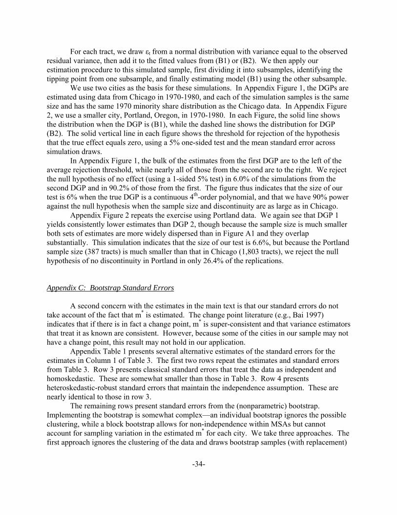
-34-

For each tract, we draw εt from a normal distribution with variance equal to the observed residual variance, then add it to the fitted values from (B1) or (B2). We then apply our estimation procedure to this simulated sample, first dividing it into subsamples, identifying the tipping point from one subsample, and finally estimating model (B1) using the other subsample.

We use two cities as the basis for these simulations. In Appendix Figure 1, the DGPs are estimated using data from Chicago in 1970-1980, and each of the simulation samples is the same size and has the same 1970 minority share distribution as the Chicago data. In Appendix Figure 2, we use a smaller city, Portland, Oregon, in 1970-1980. In each Figure, the solid line shows the distribution when the DGP is (B1), while the dashed line shows the distribution for DGP (B2). The solid vertical line in each figure shows the threshold for rejection of the hypothesis that the true effect equals zero, using a 5% one-sided test and the mean standard error across simulation draws.

In Appendix Figure 1, the bulk of the estimates from the first DGP are to the left of the average rejection threshold, while nearly all of those from the second are to the right. We reject the null hypothesis of no effect (using a 1-sided 5% test) in 6.0% of the simulations from the second DGP and in 90.2% of those from the first. The figure thus indicates that the size of our test is 6% when the true DGP is a continuous 4th-order polynomial, and that we have 90% power against the null hypothesis when the sample size and discontinuity are as large as in Chicago.

Appendix Figure 2 repeats the exercise using Portland data. We again see that DGP 1 yields consistently lower estimates than DGP 2, though because the sample size is much smaller both sets of estimates are more widely dispersed than in Figure A1 and they overlap substantially. This simulation indicates that the size of our test is 6.6%, but because the Portland sample size (387 tracts) is much smaller than that in Chicago (1,803 tracts), we reject the null hypothesis of no discontinuity in Portland in only 26.4% of the replications.

Appendix C: Bootstrap Standard Errors

A second concern with the estimates in the main text is that our standard errors do not take account of the fact that m* is estimated. The change point literature (e.g., Bai 1997) indicates that if there is in fact a change point, m* is super-consistent and that variance estimators that treat it as known are consistent. However, because some of the cities in our sample may not have a change point, this result may not hold in our application. Appendix Table 1 presents several alternative estimates of the standard errors for the estimates in Column 1 of Table 3. The first two rows repeat the estimates and standard errors from Table 3. Row 3 presents classical standard errors that treat the data as independent and homoskedastic. These are somewhat smaller than those in Table 3. Row 4 presents heteroskedastic-robust standard errors that maintain the independence assumption. These are nearly identical to those in row 3. The remaining rows present standard errors from the (nonparametric) bootstrap. Implementing the bootstrap is somewhat complex�an individual bootstrap ignores the possible clustering, while a block bootstrap allows for non-independence within MSAs but cannot account for sampling variation in the estimated m* for each city. We take three approaches. The first approach ignores the clustering of the data and draws bootstrap samples (with replacement)

-35-

from the full sample, independent of city. The second is a block bootstrap, drawing a sample of the same number of cities as in our original sample. (The number of tracts in the bootstrap samples varies somewhat here, as in some draws larger cities are overrepresented and in other draws the smaller cities are.) The final bootstrap approach is the most sophisticated. We first stratify cities into three groups: Those with fewer than 225 tracts in the sample, those with 225-999 tracts, and those with 1000 or more tracts. We perform a block bootstrap, stratifying on the city strata. This ensures a sample of the same number of cities with approximately the same size distribution as in our original sample. For each city in the bootstrap sample � treating multiple draws of the same original city as distinct � we draw with replacement from the tracts in that city to obtain a sample matching the original size. This block-and-individual bootstrap allows for both sampling variation in city-level statistics and non-independence of observations within cities. For each bootstrap strategy, on each draw we repeat our full estimation procedure. We randomly divide each city (or, in the case of the block bootstraps, city replicate) into subsamples, and use a 2/3 sample to select candidate tipping points. We then use the remaining 1/3 subsample to estimate the coefficients of our model. Rows 5-7 of Appendix Table 1 present average point estimates across 200 replications for each of the three bootstrap strategies. Those in rows 5 and 6 are comparable to those in Table 3. Those in row 7 are slightly larger than our clustered standard errors, but not enough so to change any of our qualitative conclusions.

-36-

References Andrews, Donald W. K. (1993). �Tests for Parameter Instability and Structural Change with

Unknown Change Point.� Econometrica 61 (July), pp. 821-56. Angrist, Joshua D., Guido Imbens and Alan B. Krueger (1999). �Jackknife Instrumental

Variables Estimation.� Journal of Applied Econometrics 14 (January-February), pp. 57-67.

Angrist, Johua D. and Victor C. Lavy (1999). �Using Maimonides� Rule to Estimate the Effect of Class Size on Scholastic Achievement.� Quarterly Journal of Economics 114 (May), pp. 533-575.

Bai, Jushan (1997). �Estimation of a Change Point in Multiple Regression Models.� Review of Economics and Statistics 79 (November), pp. 551�63

Bajari, Patrick, and Mathew E. Kahn (2005). �Estimating Housing Demand with an Application to Explaining Racial Segregation in Cities.� Journal of Business and Economic Statistics 23 (January), pp. 20-33.

Baum-Snow, Nathaniel (2007). �Did Highways Cause Suburbanization?� Quarterly Journal of Economics 122 (May).

Bayer, Patrick, Hanming Fang, and Robert McMillan (2005). �Separate When Equal? Racial Inequality and Residential Segregation.� National Bureau of Economic Research Working Paper #11507, October.

Bayer, Patrick, Fernando Ferreira, and Robert McMillan (2003). �A Unified Framework for Measuring Preferences for Schools and Neighborhoods.� Economic Growth Center Discussion Paper 872, Yale University, November.

Becker, Gary S. and Kevin M. Murphy (2000). Social Economics: Market Behavior in a Social Environment. Cambridge, MA: Harvard University Press/Belknap, 2000.

Bond, Eric W. and N. Edward Coulson (1989). �Externalities, Filtering, and Neighborhood Change.� Journal of Urban Economics 26 (September), pp. 231-249.

Boston, John, Leo C. Rigsby, and Mayer N. Zald (1972). �The Impact of Race on Housing Markets: A Critical Review.� Social Problems 19 (Winter), pp. 382-393.

Boustan, Leah P. (2006). �Was Postwar Suburbanization �White Flight�? Evidence from the Black Migration.� UCLA Department of Economics Unpublished Manuscript.

Brock, William A. and Steven N. Durlauf (2001a). �Discrete Choice with Social Interactions.� Review of Economic Studies 68 (April), pp. 235-260.

Brock, William A. and Steven N. Durlauf (2001b). �Interactions-Based Models.� In J. J. Heckman and E. Leamer, editors. Handbook of Econometrics, Volume 5. New York, Elsevier, pp. 3297-3380.

Carter, Gregg Lee (1986). �The 1960s Black Riots Revisited: City Level Explanations of Their Severity.� Sociological Inquiry 56 (Spring), pp. 210-228.

Case, Anne C. and Lawrence F. Katz (1991). �The Company You Keep: The Effects of Family and Neighborhood on Disadvantaged Youths.� National Bureau of Economic Research Working Paper #3705, May.

Chay, Kenneth Y. and Michael Greenstone (2005). �Does Air Quality Matter? Evidence from the Housing Market.� Journal of Political Economy 113 (April), pp. 376-424.

Clark, W. A. V. (1991). �Residential Preferences and Neighborhood Racial Segregation: A Test of the Schelling Segregation Model.� Demography 28 (February), pp. 1-19.

-37-

Clotfelter, Charles T. (1979). �Urban School Desegregation and Declines in White Enrollment: A Reexamination.� Journal of Urban Economics 6 (July), pp. 352-370.

Clotfelter, Charles T. (2001). �Are Whites Still Fleeing? Racial Patterns and Enrollment Shifts in Urban Public Schools, 1987-1996.� Journal of Policy Analysis and Management 20 (Spring), pp. 199-221.

Collins, William J. and Robert A. Margo (2004). �The Labor Market Effects of the 1960s Riots.� In W. Gale and J. Pack, editors. Brookings-Wharton Papers on Urban Affairs, 2004. Washington D.C., The Brookings Institution, pp. 1-34.

Coleman, James S., S. Kelley, and J. Moore (1975). �Trends in School Segregation, 1968-73.� Urban Institute Paper No. 772-03-91, August.

Cooper, Russell and Andrew John (1988). �Coordinating Coordination Failures in Keynesian Models.� Quarterly Journal of Economics 103 (August), pp. 441-463.

Cutler, David M., Edward L. Glaeser, and Jacob L. Vigdor (1999). �The Rise and Decline of the American Ghetto.� Journal of Political Economy 107 (June), pp. 455-506.

Downs, Anthony (1960). �An Economic Analysis of �Property Values and Race� (Laurenti).� Land Economics 36 (May), pp. 181-188.

Duncan, Otis Dudley and Beverly Duncan (1957). The Negro Population of Chicago: A Study of Residential Succession. Chicago: University of Chicago Press.

Easterly, William (2005). �Empirics of Strategic Interdependence: The Case of the Racial Tipping Point.� New York University DRI Working Paper No. 5, October.

Evans, William N., Wallace E. Oates and Robert M. Schwab (1992). �Measuring Peer Group Effects: A Study of Teenage Behavior.� Journal of Political Economy 100 (October), pp. 966-91.

Farley, Reynolds, Toni Richards, and Clarence Wurdock (1980). �School Desegregation and White Flight: An Investigation of Competing Models and Their Discrepant Findings.� Sociology of Education 53 (July), pp. 123-139.

Farley, Reynolds, Charlotte Steeh, Tara Jackson, Maria Krysan, and Keith Reeves (1993). �Continued Racial Residential Segregation in Detroit: �Chocolate City, Vanilla Suburbs� Revisited.� Journal of Housing Reseach 4 (1), pp. 1-38.

Glaeser, Edward L., Joseph Gyourko, and Raven Saks (2005). �Why Have Housing Prices Gone Up?� National Bureau of Economic Research Working Paper #11129 (February).

Glaeser, Edward, Mathew Kahn, and Jordan Rappaport (2000). �Why Do the Poor Live in Cities?� NBER Working Paper No. 7636 (April).

Glaeser, Edward L., Bruce Sacerdote, and Jose A. Scheinkman (1996). �Crime and Social Interactions.� Quarterly Journal of Economics 111 (May), pp. 507-548.

Glaeser, Edward L. and Jose A. Scheinkman (2003). �Non-Market Interactions.� In M. Dewatripont, L. P. Hansen, and S. Turnovsky, editors, Advances in Economics and Econometrics: Theory and Applications, 8th World Congress, vol. 1. Cambridge: Cambridge University Press, 2003, pp. 339-369.

Gyourko, Joseph, Christopher Mayer, and Todd Sinai (2006). �Superstar Cities.� Working paper, the Wharton School (June).

Granovetter, Mark (1978). �Threshold Models of Collective Action.� American Journal of Sociology 83 (May), pp. 1420-1443.

Graham, Brian (2005). �Identifying Social Interactions through Excess Variance Contrasts.�

-38-

University of California Berkeley, Unpublished Manuscript. May. Hahn, Jinyong, Petra Todd and Wilbert Van der Klaauw (2001). �Identification and Estimation

of Treatment Effects with a Regression Discontinuity Design.� Econometrica 69 (January), pp. 201-209.

Hansen, Bruce E. (2000). �Sample Splitting and Threshold Estimation.� Econometrica 68 (May), pp. 575-603.

Kling, Jeffrey R., Jens Ludwig and Lawrence F. Katz (2005). �Neighborhood Effects on Crime for Female and Male Youth: Evidence from a Randomized Housing Mobility Experiment.� Quarterly Journal of Economics 120 (February), pp. 87-130.

Laurenti, Luigi (1960). Property Values and Race. Berkeley: University of California Press. Leamer, Edward. (1978). Specification Searches: Ad Hoc Inference with Non Experimental

Data. New York: John Wiley and Sons. Loader, Clive R. (1996). �Change Point Estimation Using Nonparametric Regression.� Annals of

Statistics 24 (August), pp. 1667-1678. Manski, Charles F. (1993). �Identification of Endogenous Social Effects: The Reflection

Problem.� Review of Economic Studies 60 (July), pp. 531-42. Margo, Robert (1992). �Explaining the Postwar Suburbanization of Population in the United

States: The Role of Income.� Journal of Urban Economics 31, pp. 301-310. Merton, Robert K. (1948). �The Self-Fulfilling Prophecy.� Antioch Review 8, pp. 193-210. Mieszkowski, Peter, and Edwin Mills (1993). �The Causes of Metropolitan Suburbanization,�

Journal of Economic Perspectives 7 (Summer), pp. 135-147. Miyao, Takahiro (1979). �Dynamic Stability of an Open City with Many Household Classes.�

Journal of Urban Economics 6 (July), pp. 292-298. Mobius, Markus, and Tanya Rosenblat (2001). �The Process of Ghetto Formation: Evidence

from Chicago.� Manuscript, Harvard University. Myrdal, Gunnar (1948). An American Dilemma: The Negro Problem and Modern Democracy

New York: Harper & Brothers. Rapkin Chester, and William G. Grigsby (1960). The Demand for Housing in Racially Mixed

Areas. Berkeley: University of California Berkeley Press. Reber, Sarah J. (2005). �Court-Ordered Desegregation: Successes and Failures Integrating

American Schools Since Brown versus Board of Education.� Journal of Human Resources 40 (November), pp. 559-590.

Saiz, Albert and Susan Wachter. (2006). �Immigration and the Neighborhood.� Manuscript (May).

Schelling, Thomas C. (1971). �Dynamic Models of Segregation.� Journal of Mathematical Sociology 1 (July), pp. 143-186.

Schelling, Thomas C. (1978). Micromotives and Macrobehavior. New York: Norton. Schuman, Howard, Charlotte Steeh, Lawrence D. Bobo and Maria Krysan (1998). Racial

Attitudes in America: Trends and Interpretations. Cambridge: Harvard University Press. Taeuber, Karl E. and Alma F. Taeuber (1965). Negroes in Cities. Chicago: Aldine Press. Vogelmann, James E., Stephen M. Howard, Limin Yang, Charles R. Larson, Bruce K. Wylie,

and Nick Van Driel (2001), �Completion of the 1990�s National Land Cover Data Set for the Conterminous United States from Landsat Thematic Mapper Data and Ancillary Data Sources.� Photogrammetric Engineering and Remote Sensing 67 (June), pp. 650-662.

Figure 1: Neighborhood change in Chicago, 1970-1980

-60

-40

-20

020

Chan

ge in

non

-Hisp

anic

whi

te p

opul

atio

n, 1

970-

1980

0 5 10 15 20 25 30 35 40 45 50 55 60 65 70 75 80 85 90 95 100Percent minority (Hispanic or non-white) in tract in 1970

Notes: Dots show mean of the change in the tract-level non-Hispanic white population between 1970 and 1980 as a percentage of the total tract population in 1970, grouping tracts into cells of width 1% by the 1970 minority (Hispanic and/or non-white) share. The horizontal line depicts the unconditional mean. Also shown is a local linear regression fit to the tract-level data, using an Epanechnikov kernel and a bandwidth of 3.5 and estimated separately on each side of 5.7%. This point is chosen using a search procedure and a 2/3 sample of Chicago tracts. Only the remaining 1/3 subsample is used for the series depicted here. See text for details.

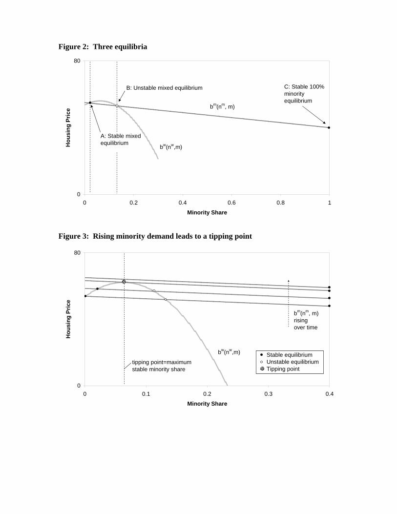
Figure 2: Three equilibria

0

80

0 0.2 0.4 0.6 0.8 1

Minority Share

Hou

sing

Pric

e bm(nm, m)

bw(nw,m)

B: Unstable mixed equilibrium

A: Stable mixedequilibrium

C: Stable 100% minorityequilibrium

Figure 3: Rising minority demand leads to a tipping point

0

80

0 0.1 0.2 0.3 0.4

Minority Share

Hou

sing

Pric

e

bm(nm, m) risingover time

bw(nw,m)

tipping point=maximumstable minority share

Stable equilibriumUnstable equilibriumTipping point

Figure 4: Neighborhood change and tipping points in several illustrative cities

-40

-20

020

40

0 20 40 60 80 100

Los Angeles-Long Beach, CA, 1970-1980

-40

-20

020

4060

0 20 40 60 80 100

Indianapolis, IN, 1970-1980-4

0-2

00

2040

60

0 20 40 60 80 100

Portland, OR-Vancouver, WA, 1970-1980

-20

020

4060

0 20 40 60 80 100

Middlesex-Somerset-Hunterdon, NJ, 1980-1990

-50

050

100

150

0 20 40 60 80 100

San Antonio, TX, 1980-1990

-40

-20

020

40

0 20 40 60 80 100

Nashville, TN, 1990-2000

-40

-20

020

0 20 40 60 80 100

Toledo, OH, 1990-2000

-40

-30

-20

-10

010

0 20 40 60 80 100

Pittsburgh, PA, 1980-1990

Note: See notes to Figure 1. Solid vertical line represents the point identified by the “fixed point” method and dashed for that selected by the “structural break” method. Where only one line is shown, the two coincide.

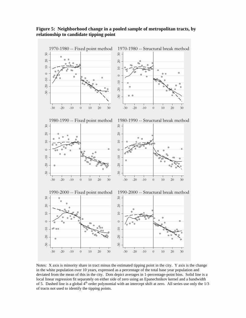
Figure 5: Neighborhood change in a pooled sample of metropolitan tracts, by relationship to candidate tipping point

-30

-20

-10

010

2030

-30 -20 -10 0 10 20 30

1970-1980 -- Fixed point method

-30

-20

-10

010

2030

-30 -20 -10 0 10 20 30

1970-1980 -- Structural break method-3

0-2

0-1

00

1020

30

-30 -20 -10 0 10 20 30

1980-1990 -- Fixed point method-3

0-2

0-1

00

1020

30

-30 -20 -10 0 10 20 30

1980-1990 -- Structural break method

-30

-20

-10

010

2030

-30 -20 -10 0 10 20 30

1990-2000 -- Fixed point method

-30

-20

-10

010

2030

-30 -20 -10 0 10 20 30

1990-2000 -- Structural break method

Notes: X axis is minority share in tract minus the estimated tipping point in the city. Y axis is the change in the white population over 10 years, expressed as a percentage of the total base year population and deviated from the mean of this in the city. Dots depict averages in 1-percentage-point bins. Solid line is a local linear regression fit separately on either side of zero using an Epanechnikov kernel and a bandwidth of 5. Dashed line is a global 4th order polynomial with an intercept shift at zero. All series use only the 1/3 of tracts not used to identify the tipping points.

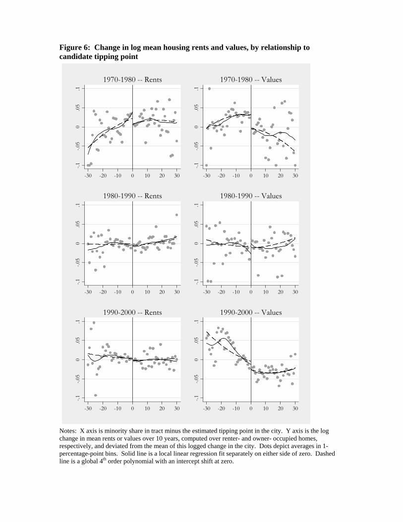
Figure 6: Change in log mean housing rents and values, by relationship to candidate tipping point

-.1-.0

50

.05

.1

-30 -20 -10 0 10 20 30

1970-1980 -- Rents

-.1-.0

50

.05

.1

-30 -20 -10 0 10 20 30

1970-1980 -- Values-.1

-.05

0.0

5.1

-30 -20 -10 0 10 20 30

1980-1990 -- Rents-.1

-.05

0.0

5.1

-30 -20 -10 0 10 20 30

1980-1990 -- Values

-.1-.0

50

.05

.1

-30 -20 -10 0 10 20 30

1990-2000 -- Rents

-.1-.0

50

.05

.1

-30 -20 -10 0 10 20 30

1990-2000 -- Values

Notes: X axis is minority share in tract minus the estimated tipping point in the city. Y axis is the log change in mean rents or values over 10 years, computed over renter- and owner- occupied homes, respectively, and deviated from the mean of this logged change in the city. Dots depict averages in 1-percentage-point bins. Solid line is a local linear regression fit separately on either side of zero. Dashed line is a global 4th order polynomial with an intercept shift at zero.

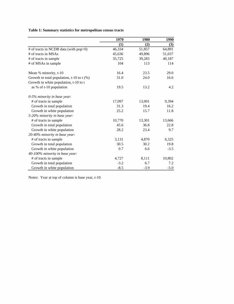
Table 1: Summary statistics for metropolitan census tracts

1970 1980 1990(1) (2) (3)

# of tracts in NCDB data (with pop>0) 46,334 51,857 64,891# of tracts in MSAs 45,636 49,896 51,037# of tracts in sample 35,725 39,283 40,187# of MSAs in sample 104 113 114

Mean % minority, t-10 16.4 23.5 29.0Growth in total population, t-10 to t (%) 31.0 24.0 16.6Growth in white population, t-10 to t

as % of t-10 population 19.5 13.2 4.2

0-5% minority in base year:# of tracts in sample 17,097 13,001 9,394Growth in total population 31.3 19.4 16.2Growth in white population 25.2 15.7 11.8

5-20% minority in base year:# of tracts in sample 10,770 13,301 13,666Growth in total population 45.6 36.8 22.8Growth in white population 28.2 23.4 9.7

20-40% minority in base year:# of tracts in sample 3,131 4,870 6,325Growth in total population 30.5 30.2 19.8Growth in white population 0.7 6.6 -3.5

40-100% minority in base year:# of tracts in sample 4,727 8,111 10,802Growth in total population -3.2 6.7 7.2Growth in white population -8.5 -3.9 -5.0

Notes: Year at top of column is base year, t-10.

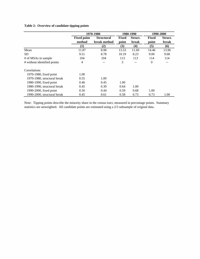
Table 2: Overview of candidate tipping points

Fixed point method

Structural break method

Fixed point

Struct. break

Fixed point

Struct. break

(1) (2) (3) (4) (5) (6)Mean 11.87 8.98 13.53 11.69 14.46 13.96SD 9.51 8.78 10.19 8.23 9.00 9.68# of MSAs in sample 104 104 113 113 114 114# without identified points 4 -- 3 -- 0 --

Correlations1970-1980, fixed point 1.001970-1980, structural break 0.55 1.001980-1990, fixed point 0.46 0.45 1.001980-1990, structural break 0.45 0.39 0.64 1.001990-2000, fixed point 0.50 0.44 0.59 0.68 1.001990-2000, structural break 0.45 0.61 0.58 0.73 0.73 1.00

1990-20001970-1980 1980-1990

Note: Tipping points describe the minority share in the census tract, measured in percentage points. Summary statistics are unweighted. All candidate points are estimated using a 2/3 subsample of original data.

Fixed point

Structural break

Fixed point

Struct. break

Fixed point

Struct. break

Fixed point

Struct. break

(1) (2) (3) (4) (5) (6) (7) (8)1970-1980

Beyond candidate tipping -12.1 -10.4 -14.2 -16.4 2.0 -0.1 -10.1 -10.4 point in 1970 (2.7) (3.4) (3.1) (4.3) (1.0) (1.2) (3.0) (3.5)Demographic/housing controls y y n n y y y yN 11,611 11,886 11,611 11,886 11,611 11,886R2 0.25 0.25 0.22 0.22 0.23 0.24

1980-1990Beyond candidate tipping -13.6 -11.4 -17.0 -18.6 -1.1 0.3 -14.7 -11.1 point in 1980 (2.0) (3.5) (3.1) (3.5) (1.1) (1.1) (2.6) (4.1)N 12,151 13,067 12,151 13,067 12,151 13,067R2 0.30 0.30 0.26 0.26 0.29 0.29

1990-2000Beyond candidate tipping -7.3 -9.3 -3.6 -6.6 2.9 1.4 -4.3 -7.9 point in 1990 (1.5) (1.8) (2.1) (2.0) (1.1) (0.8) (2.1) (2.2)N 13,371 13,371 13,371 13,371 13,371 13,371R2 0.15 0.14 0.18 0.19 0.13 0.13

Table 3: Basic regression discontinuity models for population changes around the candidate tipping point

Notes: The unit of observation is a tract in the indicated decade. Dependent variables are the change in the relevant population (white in columns 1-4, minority in 5-6, or total in 7-8) as a percentage (0-100) of the tract's total base-year population. Pooled specifications (columns 1-2 and 5-8) include MSA fixed effects, a quartic polynomial in the deviation in the tract’s minority share from the candidate tipping point, the unemployment rate, log(mean family income), housing vacancy rate, renter share, fraction of homes in single-unit buildings, and fraction of workers who commute using public transit, all measured in the base year at the tract-level. Standard errors are clustered on the MSA. Fully interacted specifications (columns 3-4) report average tipping coefficients from city-by-city regressions with quartics in the tract minority share. The coefficient on the "beyond tipping point" indicator is averaged across cities, weighing cities by their numbers of tracts. Standard errors in these columns are robust to heteroskedasticity. All specifications are estimated using only the 1/3 of tracts not used to identify the tipping points.

Change in white population Change in minority pop.

Change in total population

Fully interactedPooled Pooled Pooled

Table 4: Tipping in the 1990s, by amount of remaining undeveloped land

# of tracts Change in white population

Change in minority population

Change in total population

Change in minority share

(1) (2) (3) (4) (5)Full sample 13,371 -7.3 2.9 -4.3 3.4

(1.5) (1.1) (2.1) (0.4)>91% developed 3,368 -4.7 4.7 0.0 4.6

(1.1) (1.1) (1.3) (1.0)<91% developed 9,875 -6.1 2.4 -3.7 2.5

(1.8) (1.3) (2.6) (0.4)

Note: See notes to Table 3 (columns 1, 5, and 7) for details on sample and specifications. Fixed point candidate tipping points are used. Column 5 takes as the dependent variable the minority share in 2000 minus the minority share in 1990, but is otherwise identical. Developed land measure is computed from the National Land Cover Data; 91% is the 75th percentile of this measure. See text for details.

Tipping discontinuity, 1990-2000

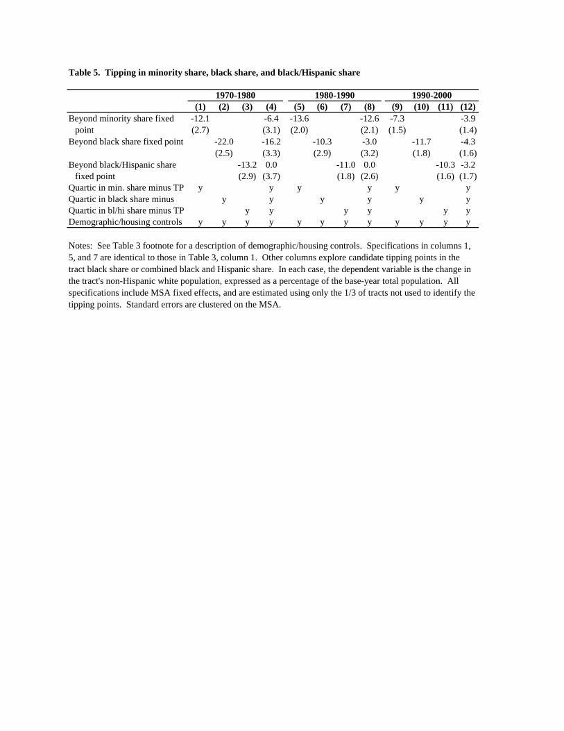
Table 5. Tipping in minority share, black share, and black/Hispanic share

(1) (2) (3) (4) (5) (6) (7) (8) (9) (10) (11) (12)-12.1 -6.4 -13.6 -12.6 -7.3 -3.9

point (2.7) (3.1) (2.0) (2.1) (1.5) (1.4)-22.0 -16.2 -10.3 -3.0 -11.7 -4.3(2.5) (3.3) (2.9) (3.2) (1.8) (1.6)

-13.2 0.0 -11.0 0.0 -10.3 -3.2fixed point (2.9) (3.7) (1.8) (2.6) (1.6) (1.7)

y y y y y yy y y y y y

y y y y y yy y y y y y y y y y y y

Notes: See Table 3 footnote for a description of demographic/housing controls. Specifications in columns 1, 5, and 7 are identical to those in Table 3, column 1. Other columns explore candidate tipping points in the tract black share or combined black and Hispanic share. In each case, the dependent variable is the change in the tract's non-Hispanic white population, expressed as a percentage of the base-year total population. All specifications include MSA fixed effects, and are estimated using only the 1/3 of tracts not used to identify the tipping points. Standard errors are clustered on the MSA.

Beyond minority share fixed

Beyond black/Hispanic share

Beyond black share fixed point

Quartic in bl/hi share minus TPDemographic/housing controls

Quartic in min. share minus TPQuartic in black share minus

1990-20001980-19901970-1980

Table 6. Sensitivity to flexible controls for neighborhood demographics

(1) (2) (3) (4) (5) (6) (7)1970-1980 -12.1 -12.2 -12.2 -12.7 -11.3 -12.7 -12.1

(2.7) (2.7) (2.7) (2.7) (2.6) (2.7) (2.6)4th order polynomial in:

Unemployment rate y ylog(mean family income) y yVacancy rate y yRenter share y yFraction single-unit buildings y y

1980-1990 -13.6 -13.3 -13.3 -13.6 -12.6 -13.6 -11.8(2.0) (2.0) (2.0) (2.0) (2.0) (2.0) (2.0)

1990-2000 -7.3 -7.0 -7.1 -7.5 -6.0 -6.9 -5.5(1.5) (1.5) (1.5) (1.5) (1.5) (1.5) (1.5)

Notes: Specification in column 1 is that from column 1 of Table 3. Remaining specifications add quartic polynomials in the listed control variables.

Table 7. Variation in discontinuity at the tipping point by measures of distance to the existing ghetto

1970-1980

1980-1990

1990-2000

1970-1980

1980-1990

1990-2000

1970-1980

1980-1990

1990-2000

(1) (2) (3) (4) (5) (6) (7) (8) (9)-10.7 -10.6 -4.9 -7.6 -4.7 -3.4 -0.6 -2.7 -3.4(3.5) (2.5) (2.2) (2.2) (2.7) (1.2) (3.0) (2.2) (1.4)3.0 -5.9 -2.5

(5.1) (4.6) (2.8)-7.7 -16.5 -7.3(3.4) (3.8) (2.1)

-3.9 5.1 0.1(5.3) (5.3) (2.3)-2.6 -15.9 0.6(4.4) (4.8) (2.9)-11.5 0.5 -3.3(5.1) (4.1) (1.9)-10.3 -20.6 -2.8(3.8) (3.7) (2.6)

-30.3 -31.8 -2.1(7.0) (4.7) (5.4)-30.9 -34.5 -5.4(6.3) (4.6) (5.2)

Notes: Specifications are identical to those in Table 3, Column 1, but are fully interacted with the indicated tract characteristics. Reported here are the beyond-tipping-point main effects, interaction coefficients, and the net effect of being beyond the tipping point for tracts in each category. The nearest high-minority-tract is the closest tract (measuring distances between tract centroids) with a minority share above 60%. "Neighbors" in columns 7-9 are the five closest tracts within five miles.

Total tipping effect when distance is 2-5 miles

Interaction: Beyond TP x none of neighbors have m>m*

Total tipping effect when none of neighbors have m>m*

By central city / remainder of MSA

By indicator for having a neighbor

with m>m*

By distance to nearest high-

minority share

Total tipping effect when distance is >5 miles

Interaction: Beyond TP x outside of central city

Total tipping effect when outside of central city

Main effect: Beyond tipping point

Interaction: Beyond TP x nearest high-minority-share tract is 2-5 miles awayInteraction: Beyond TP x nearest high-minority-share tract is >5 miles away

Table 8: Tipping in elementary schools

Change in white population

Change in minority population

Change in total population

Change in minority share

(2) (3) (4) (5)Beyond candidate -7.4 0.9 -6.5 2.3

tipping point (2.3) (0.9) (2.3) (0.8)N 5,641 5,641 5,641 5,641

Note: Sample consists of elementary schools in the MSA. Tipping points are estimated using the fixed point method over a 2/3 subsample; the remaining 1/3 subsample is used to estimate the specifications shown here. Each includes a quartic polynomial in the minority share relative to the candidate tipping point, MSA fixed effects, and a control for the school free lunch share. Standard errors are clustered on the MSA.

Tipping discontinuity, 1990-2000

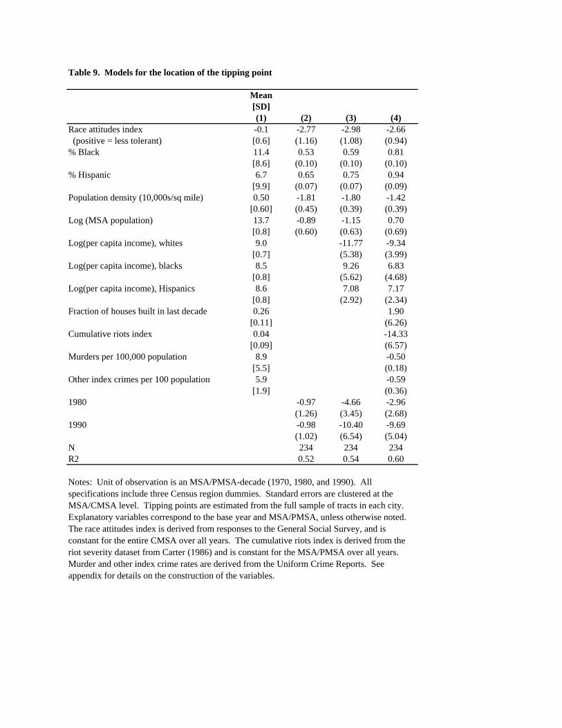
Table 9. Models for the location of the tipping point

Mean[SD](1) (2) (3) (4)

Race attitudes index -0.1 -2.77 -2.98 -2.66 (positive = less tolerant) [0.6] (1.16) (1.08) (0.94)% Black 11.4 0.53 0.59 0.81

[8.6] (0.10) (0.10) (0.10)% Hispanic 6.7 0.65 0.75 0.94

[9.9] (0.07) (0.07) (0.09)Population density (10,000s/sq mile) 0.50 -1.81 -1.80 -1.42

[0.60] (0.45) (0.39) (0.39)Log (MSA population) 13.7 -0.89 -1.15 0.70

[0.8] (0.60) (0.63) (0.69)Log(per capita income), whites 9.0 -11.77 -9.34

[0.7] (5.38) (3.99)Log(per capita income), blacks 8.5 9.26 6.83

[0.8] (5.62) (4.68)Log(per capita income), Hispanics 8.6 7.08 7.17

[0.8] (2.92) (2.34)Fraction of houses built in last decade 0.26 1.90

[0.11] (6.26)Cumulative riots index 0.04 -14.33

[0.09] (6.57)Murders per 100,000 population 8.9 -0.50

[5.5] (0.18)Other index crimes per 100 population 5.9 -0.59

[1.9] (0.36)1980 -0.97 -4.66 -2.96

(1.26) (3.45) (2.68)1990 -0.98 -10.40 -9.69

(1.02) (6.54) (5.04)N 234 234 234R2 0.52 0.54 0.60

Notes: Unit of observation is an MSA/PMSA-decade (1970, 1980, and 1990). All specifications include three Census region dummies. Standard errors are clustered at the MSA/CMSA level. Tipping points are estimated from the full sample of tracts in each city. Explanatory variables correspond to the base year and MSA/PMSA, unless otherwise noted. The race attitudes index is derived from responses to the General Social Survey, and is constant for the entire CMSA over all years. The cumulative riots index is derived from the riot severity dataset from Carter (1986) and is constant for the MSA/PMSA over all years. Murder and other index crime rates are derived from the Uniform Crime Reports. See appendix for details on the construction of the variables.

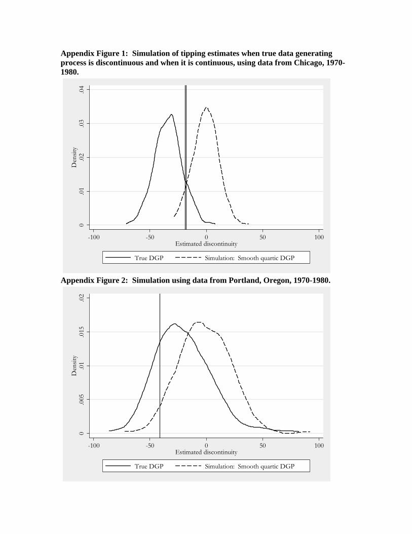
Appendix Figure 1: Simulation of tipping estimates when true data generating process is discontinuous and when it is continuous, using data from Chicago, 1970-1980.

0.0

1.0

2.0

3.0

4D

ensit

y

-100 -50 0 50 100Estimated discontinuity

True DGP Simulation: Smooth quartic DGP

Appendix Figure 2: Simulation using data from Portland, Oregon, 1970-1980.

0.0

05.0

1.0

15.0

2D

ensit

y

-100 -50 0 50 100Estimated discontinuity

True DGP Simulation: Smooth quartic DGP

Appendix Table 1: Bootstrap vs. regular SEs

1970s 1980s 1990s(1) Coefficient estimate -12.15 -13.63 -7.26(2) SE: Cluster 2.73 2.02 1.53(3) SE: Classical 2.21 1.63 1.22(4) SE: Robust 2.15 1.67 1.23(5) SE: Bootstrap 2.27 1.49 1.09(6) SE: Block bootstrap 2.51 2.22 1.52(7) SE: Block and individual bootstrap 2.99 2.29 1.72

Notes: Point estimates in row 1 and standard errors in row 2 are from Column 1 of Table 3. Remaining rows report standard errors from various alternative estimators.