©2015 UL/Streyler/RTaW 1/12

Timing verification of real­time automotive Ethernet networks:

what can we expect from simulation?

Nicolas Navet, University of Luxembourg

Jan R. Seyler1, Streyler GbR, Germany

Jörn Migge, RealTime-at-Work, France

Abstract: Switched Ethernet is a technology that is profoundly reshaping automotive communication

architectures as it did in other application domains such as avionics with the use of AFDX backbones. Early

stage timing verification of critical embedded networks typically relies on simulation and worst-case

schedulability analysis. When the modeling power of schedulability analysis is not sufficient, there are

typically two options: either make pessimistic assumptions or ignore what cannot be modeled. Both options

are unsatisfactory because they are either inefficient in terms of resource usage or potentially unsafe. To

overcome those issues, we believe it is a good practice to use simulation models, which can be more

realistic, along with schedulability analysis. The two basic questions that we aim to study here is what can

we expect from simulation, and how to use it properly? This empirical study explores these questions on

realistic case-studies and provides methodological guidelines for the use of simulation in the design of

switched Ethernet networks. A broader objective of the study is to compare the outcomes of schedulability

analyses and simulation, and conclude about the scope of usability of simulation in the desi gn of critical

Ethernet networks.

Keywords: timing verification, timing-accurate simulation, ergodicity, automotive Ethernet, simulation

methodology, worst-case response time analysis.

1 C on t ext an d ob ject i ve s o f th e s tud y

Ethernet is meant in vehicles not only for the support of infotainment applications but also to transmit time-

sensitive data used for the real-time control of the vehicle and ADAS functions. In such use -cases, the

temporal behavior of the communication architecture must be carefully validated. Early stage timing

verification of critical embedded networks typically relies on simulation and worst -case schedulability

analysis, which basically consists in building a mathematical model of the worst possible situations that can

be encountered at run-time.

When the modeling capabilities of schedulability analysis is not sufficient, which given the complexity of

today’s architectures is in our experience in many practical situations the case (see [Na13,Na14] and § 2.4),

there are typically two possibilities. The first option is to make pessimistic assumptions (e.g., modeling

aperiodic frames as periodic ones), which is not always possible because for instance it may result in

overloaded resources (e.g., link utilization larger than 100%) . The second option is to ignore what cannot be

modeled (e.g., ignoring transmission errors, aperiodic traffic, etc). Both options are unsatisfactory because

they are either inefficient in terms of resource usage or potentially unsafe. In addition, it can happen that

schedulability analysis tools provide wrong results, most often because the analysis’ assumptions are not

met by the actual implementation, or possibly because of numerical issues in the implementation (e.g., if

floating point arithmetic is used), or simply because the analysis is flawed (see for instance [Da07]).

To overcome these issues, we believe that it is needed to use simulation along with schedulability analysis,

so that the results of the two techniques can be cross -validated. Compared to schedulability analysis

models, simulation models can be more realistic since it is feasible for a network simulator to capture all

timing-relevant characteristics of the communication architecture and reproduce complex traffic patterns

specific to

o A higher-level protocol such as SOME/IP SD [Sey15], or the many different frame triggering

conditions in AUTOSAR Socket Adapter (see [SoAd] §7.2.2),

o An applicative-level software component.

The main shortcoming of simulation is that it does not provide any guarantees on the relevance of the

results, and the user remains always unsure about the extent to which simulation results can be trusted.

1 Jan Seyler was at Daimler AG, Mercedes-Benz Cars Development, at the time the study was conducted. An oral -only presentation

with the same title was given at SAE World Congress 2015, "Safety-Critical Systems" Session, Detroit, USA, April 21-23, 2015.

©2015 UL/Streyler/RTaW 2/12

Simulation can lead to wrong decisions because of mistakes in methodology (e.g, simulation time, number

of experiments, etc) or simply because the performance metrics under study are just out-of-reach of

simulation. The two basic questions that we aim to study here is what can we expect from simulation , and

how to use it properly? This empirical study explores these questions a nd provides methodological

guidelines for the use of simulation in the design of switched Ethernet networks. A broader objective of the

study is to compare the outcomes of schedulability analyses and simulation, and conclude about the scope

of usability of simulation in the design of critical Ethernet networks.

We paid a special attention in this study that the models used in simulation and schedulability analysis are

in line, which means that they model the same characteristics of the system and make the s ame set of

simplifying assumptions (see §2.1) regarding behaviors of the system that we believe are not central in this

study. In many practical cases, this will however not be the case because the schedulability analyses

available today are not able to capture the whole complexity of most communication architectures.

The article is organized as follows. We first study the following methodological questions:

o Q1: is a single simulation run enough or should the statistics be made out of several simulations

with different initial conditions since simulation results depend on the initial conditions?

o Q2: can we run several simulations in parallel and aggregate the results?

o Q3: what is the appropriate minimum simulation length?

Answering these three questions first requires to know whether the simulated system is ergodic (see §3.1)

or not. We then assess the scope of usability of simulation by comparison with schedulability analysis, and

explore the followings questions:

o Q4: are the latency upper-bounds derived by schedulability analysis, based on the state of the art of

the Network Calculus, as used in this study, accurate wrt to the latencies that can actually occur in

the worst-case?

o Q5: is simulation an appropriate technique to derive the worst-case communication latencies?

2 E xp er i men ta l s e tup

2.1 System under study and assumptions

In this work, we consider a standard switched Ethernet network supporting uni- and multicast

communication between a set of software components distributed on a number of stations. In the following,

the terms flow or streams refer to the data sent to a certain receiver of a multicast connection; all packets,

also called frames, of the same traffic flow are delivered over the same path.

In order to identify the primary impacting factors, the following set of assumptions is placed:

o The exact architecture of the communication stacks is not considered (e.g, AUTOSAR

communication stack). It is assumed that frames are waiting for transmission in a queue sorted by

frame priorities then arrival times. If packets have no priority, as in case-study #2, the waiting

queue is FIFO,

o The routing of the packets to the destination nodes is static,

o It is assumed that there are no transmission errors,

o Nodes’ clocks are drifting away with the clock drifts being random but constant over time (see

§2.6). The clock drift rates used in the experiments (±200ppm and ±400ppm) are realistic in the

automotive domain [Na12],

o There are no buffer overflows in the Ethernet switches which would cause packets to be lost. In

practice, this has to be avoided and can be ascertained by schedulability analysis, or, with a high

confidence, by simulation,

o The packet switching delays in the Ethernet communication switches is assumed to be upper

bounded, and vary from packet to packet according to a uniform distribution in the interval [0.1*

bound, bound],

o Streams of frames are periodic and the successive frames of a stream are all of the same size,

o The communication switches are all store-and-forward switches.

©2015 UL/Streyler/RTaW 3/12

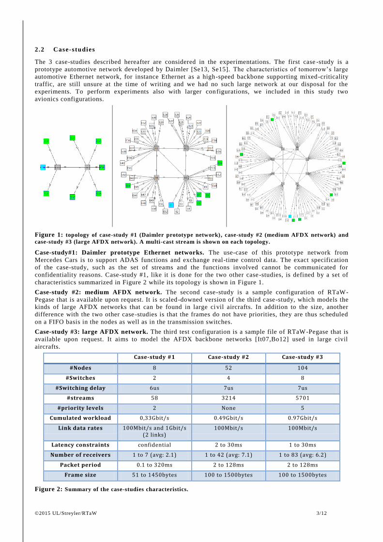
2.2 Case-studies

The 3 case-studies described hereafter are considered in the experimentations. The first case -study is a

prototype automotive network developed by Daimler [Se13, Se15]. The characteristics of tomorrow’s large

automotive Ethernet network, for instance Ethernet as a high-speed backbone supporting mixed-criticality

traffic, are still unsure at the time of writing and we had no such large network at our disposal for the

experiments. To perform experiments also with larger con figurations, we included in this study two

avionics configurations.

Figure 1: topology of case-study #1 (Daimler prototype network), case-study #2 (medium AFDX network) and

case-study #3 (large AFDX network). A multi-cast stream is shown on each topology.

Case-study#1: Daimler prototype Ethernet networks. The use-case of this prototype network from

Mercedes Cars is to support ADAS functions and exchange real-time control data. The exact specification

of the case-study, such as the set of streams and the functions involved cannot be communicated for

confidentiality reasons. Case-study #1, like it is done for the two other case-studies, is defined by a set of

characteristics summarized in Figure 2 while its topology is shown in Figure 1.

Case-study #2: medium AFDX network. The second case-study is a sample configuration of RTaW-

Pegase that is available upon request. It is scaled-downed version of the third case-study, which models the

kinds of large AFDX networks that can be found in large ci vil aircrafts. In addition to the size, another

difference with the two other case-studies is that the frames do not have priorities, they are thus scheduled

on a FIFO basis in the nodes as well as in the transmission switches.

Case-study #3: large AFDX network. The third test configuration is a sample file of RTaW-Pegase that is

available upon request. It aims to model the AFDX backbone networks [It07,Bo12] used in large civil

aircrafts.

Case-study #1 Case-study #2 Case-study #3

#Nodes 8 52 104

#Switches 2 4 8

#Switching delay 6us 7us 7us

#streams 58 3214 5701

#priority levels 2 None 5

Cumulated workload 0,33Gbit/s 0.49Gbit/s 0.97Gbit/s

Link data rates 100Mbit/s and 1Gbit/s (2 links)

100Mbit/s 100Mbit/s

Latency constraints confidential 2 to 30ms 1 to 30ms

Number of receivers 1 to 7 (avg: 2.1) 1 to 42 (avg: 7.1) 1 to 83 (avg: 6.2)

Packet period 0.1 to 320ms 2 to 128ms 2 to 128ms

Frame size 51 to 1450bytes 100 to 1500bytes 100 to 1500bytes

Figure 2: Summary of the case-studies characteristics.

©2015 UL/Streyler/RTaW 4/12

Due to space constraints, the results are not always shown in this paper for all the configurations. The

reader is referred to [Na15] for the complete set of experimental results.

2.3 Software Toolset and performance evaluation techniques

This study has been conducted using RTaW-Pegase 2.1.7 timing analysis software, a product of RealTime-

at-Work developed in partnership with ONERA research lab. RTaW-Pegase provides:

o Timing-accurate simulation . Conceptually, at each step n of the simulation, the system is fully

characterized by a state Sn and the set of rules to change from state n to n+1: Sn+1 = F( Sn+1) is

defined by the simulation model. The evolution of the system depends on this set of rules and the

sequence of values provided by the random generator.

o Worst-case latencies (i.e., worst-case response times calculation) using a state-of-the-art network

calculus implementation [Bo11]. The pessimism of this schedulability analysis is known to be

limited as it has been experimentally evidenced in the non-prioritized case in [Bo12] and in the

experiments of §4.1,

o Lower-bound on the worst-case latencies. This information is key to estimate how tight the

schedulability analysis is. The algorithm implemented in RTaW-Pegase is based on [Ba10].

Simulation results are of course much more fine-grained since the distributions of all quantities of interest

can be collected during simulation runs. In the experiments of this study, the simulator is able to compute

about 4.1 mega events per second on a single core of a standard desktop workstation (Intel I7-2600K

3.4Ghz), which means for instance that it can simulate 24 hours of communication for the first case-study in

about 1h57mn, or less than 15mn with 8 simulations executed in parallel on a 8 core machines. This speed

of execution is achieved by abstracting away all characteristics of the system without impact on its timing

behavior. Speed is indeed crucial for simulation used in the design of critical systems since the samples of

values collected must be sufficiently large to derive robust statistics with respect to the criticality of the

application (i.e., samples sufficiently large for 1-10-5

quantile values, see [Na14]). Schedulability analysis

is much faster that simulation, it takes about 15 seconds for the largest case-studies on the workstation used

in the experiments. This speed of execution can be explained firstly because Network Calculus scales

extremely well due to its low algorithmic complexity, and also because the implementation has been

optimized since it has been started to be developed in 2009 in the P egase collaborative project, see [Bo11].

2.4 Why schedulabil ity analysis alone i s not suff ic ient

Worst-case response time (WCRT) analysis, also referred to as schedulability analysis, is often considered

as the technique that is the best suited to provide the guarantees that are needed in critical networks.

Indeed, as soon as the workload submitted is bounded and the resource behaves in a deterministic manner,

then it is always possible in theory to derive a worst-case schedulability analysis. Our experience with

schedulability analyses has been however that they suffer from limitations in many practical cases due to

the following issues:

1. Pessimism due to coarse-grained or conservative models (e.g., as in [Da12]) potentially leading to

hardware resource over-provisioning. This might even rule out the use of analytic techniques in

contexts where resource usage optimization is an industrial requirement,

2. Complexity that makes them error prone and hard to validate, especially since the analytic models

used are most often not published2 and the software implementing them is a black-box for the user,

3. The inability to capture today’s complex software and hardware architectures. Using an inaccurate

model can lead to inefficient resource usage or even unsafe design choices. What makes this

perhaps the biggest issue is that it is hardly possible to foresee the effect of simplifying

assumptions, given the non-monotonous and non-linear behavior of the model outputs.

An illustration of the latter point is that at the time of writing there is, as far as we know, no schedulability

analysis that captures the complex frame transmission policies in the AUTOSAR Socket Adapter behavior

[SaAd15], while simulation of this component is readily available in RTaW -Pegase for instance. Here we do

not mean that schedulability analysis is never an appropriate technique, but simply that it is best suited to

systems which have designed and implemented with simplicity, determinism and analyzability as primary

design objectives. The reader can refer to [Na13, Na14] for a more thorough discussion on the

complementarities of verification techniques in the design of automotive communication architectures.

2 The core timing analysis algorithms of RTaW-Pegase have been published, e.g. [Bo07,Bo11], and partly formally proven in

[Ma13,Bo14b].

©2015 UL/Streyler/RTaW 5/12

2.5 Rando mness in the simulat ion

Our simulation model of the Ethernet communication system is stochastic in the sense that two different

simulation runs of the same configuration will not lead to the exact same tr ajectory of the system. Under the

assumptions made in this study (e.g., no transmission errors , fixed packet size and period) the randomness

comes entirely from:

o the offsets of the nodes, which is the initial time (wrt the network’s origin of time) at which the

nodes start to send messages (e.g., not all nodes will start to transmit simultaneously because of

different boot times),

o the clock drifts of the nodes: the clocks that drive all activities on their host processor including the

communication, do not operate at the exact same frequency,

o the switch commutation delay, that is the time it takes to copy a frame from its input port to a

waiting queue on the output port.

These characteristics of the system are drawn at random according to the p arameter ranges specified by the

user (e.g, ±200 ppm maximum for the clock drifts) , and their exact value depends on the seed of the random

generator that is used for the simulation.

2.6 Modeling c lock-drift s

The clocks of the CPUs of the network nodes never operate exactly at the same rate and thus they are

slowly drifting away. These clock drifts result from various factors, the main ones being fabrication

tolerance, aging and temperature (see [Mo12] for a discussion of the main factors of clock drifts and their

quantification in automotive systems). Clock drifts are measured in “parts per million” or ppm, which

expresses how slower or faster a clock is, as compared to a “perfect” clock. For instance, 1ppm corresponds

to a deviation of 1µs every second. In this study, we assume that clocks drifts are constant throughout the

simulation run and use the same model as in [Mo12]. For a given clock c driving an Ethernet node, its local

time tc with respect to a global time t is determined as follows in the simulation model : tc (t) = φc + δc · t

where φc is the initial start time (the offset) of the node with regard to the bus time referential, and δc is

the constant drift value. For instance, a drift rate of +100ppm means that δc = 1.0001. In this work, every

node j is assigned a clock defined by the tuple (φj , δj) which is chosen at random according the simulation

parameters.

2.7 Performance metr ics for fra me latencies

The main performance metric for real-time communication networks is the communication latency, also

called frame response time, which is the time from the production of a message until the reception by the

stations that consume the message. The latency constraint, or deadline constraint, is the maximum allowed

value for the response time. This deadline is typically inherited from applicative level constraints or

regulatory constraints (e.g. , time to answer a diagnosis request).

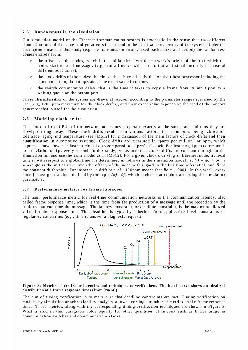
Figure 3: Metrics of the frame latencies and techniques to verify them. The black curve shows an idealized

distribution of a frame response times (from [Na14]).

The aim of timing verification is to make sure that deadline constraints are met. Timing verification on

models, by simulation or schedulability analysis, allows deriv ing a number of metrics on the frame response

times. Those metrics, along with the corresponding timing verification techniques are shown in Figure 3.

What is said in this paragraph holds equally for other quantities of interest such as buffer usage in

communication switches and communications stacks.

©2015 UL/Streyler/RTaW 6/12

The bound on the response time, which is the outcome of a schedulability analysis, is usually larger than the

true worst-case possible response time (denoted by WCRT). In general schedulability analysis is pessimistic

to an extent that cannot be predicted. However, in some cases it is possible to derive lower-bounds on the

WCRT based on a pessimistic trajectory of the system that we know can happen. This is an analysis

performed in §4.1. The maximum value seen during a simulation is most often less than the WCRT, here

again the distance between both values is unknown and depends on the network configuration as shown in

the experiments of §4.2. In the context of networks, the WCRT is also sometimes referred to as Worst -Case

Traversal Time (WCTT), this is the term used in the rest of this document.

In the design phase, the quantiles of the quantities of interest are often other meaningful performance

metrics. Formally, for a random variable X, a p-quantile is the smallest value x such that P[X>x] < 1- p. In

other words, it is a threshold L such that for any response time,

o the probability to be smaller than L is larger than p,

o the probability to be larger than L is smaller than 1 – p.

For example, the probability that a response-time is larger than the (1-10-3

)-quantile, denoted here by Q3

quantile or Q3 for short, is lower than 10-3

. For a frame with a period of 10ms, the Q3 will be exceeded on

average once every 103·10ms=10

4ms, that is 10s. Table 1 shows how quantiles translate to deadline miss

frequency and average time between deadline misses, for frames with a period equal to 10ms and 500ms

and deadlines assumed to be equal to quantiles.

Quantile Deadline miss every Mean time to deadline miss if period is 10ms

Mean time to deadline miss if period is 500ms

Q3 1000 10 s 8mn 20s

Q4 10 000 1mn 40s ≈ 1h 23mn

Q5 100 000 ≈ 17mn ≈ 13h 53mn

Q6 1000 000 ≈ 2h 46mn ≈ 5d 19h

Table 1: Quantiles and corresponding frame deadline miss frequencies for frame periods equal to 10ms and

500ms, and frame deadlines assumed to be equal to quantiles values (from [Na14]).

As exemplified in [Na14], verifying timing constraints with quantiles involves the following steps:

1. Identify the deadline for each frame,

2. With respect to the deadline miss probability that can be tolerated by the application, set the target

quantile for each frame,

3. The objective is met if the target quantile value derived by simulation is below the frame deadline.

3 Met hod ol og y and p a ra met er s f or s imu l a t ion

In this section we explore the following questions pertaining to the choice of a proper methodology and

setup for simulation:

o Q1: is a single simulation run enough or should the statisti cs be made out of several simulations

with different initial conditions since simulation results depend on the initial conditions?

o Q2: can we run several simulations in parallel and aggregate the results?

o Q3: what is the appropriate minimum simulation length?

Answering these three questions requires first to know whether the simulated system is ergodic.

In the simulations performed in this work, except if otherwise stated, the following set of parameters was

used:

o The clock drift of each node is chosen at random in ±200ppm. Simulations performed with

±400ppm returned results that were not significantly different,

o The offsets of the nodes are chosen at random in [0,100ms]. Simulations performed with offsets in

[0,1s] returned results that were not significantly different,

o Each experiment is repeated 10 times with random offsets and clock drifts,

o Simulation time was at least 2 days of functioning time, corresponding to samples with more than

20 values above Q5 for sub-90ms flows.

©2015 UL/Streyler/RTaW 7/12

3.1 Ergodicity of a dyna mic process and practical impl icat ions

Intuitively, a dynamic system is said to be ergodic if, after a certain time, every trajectory of the system

leads the same distribution of the state of the system, called the equilibrium state. If the system that is

simulated is ergodic, it means that all statistical information can be derived from one sufficiently long

simulation, since all simulations cover the state space of the system in a “similar” manner.

A single simulation of an ergodic system, or a few shorter simulations executed in parallel on a multicore

machine, will lead to the same results as a large number of simulations with different initial conditions.

This means from a practical point that we do not have to care about the number of distinct experiments that

are to be performed, as long as each of them are “sufficiently” long, and the results obtained hold whatever

the exact initial conditions of the system are.

The question that is experimentally investigated next is whether the ergodic property holds true or not for

the system under study. In the latter case, this would imply that we would need to examine a large number

of trajectories of the system, as done in the analytic techniques to calculate frame response time distribution

in AFDX [Mau13] and CAN [Ze09, Ze10].

3.2 Do init ial condit ions have an impact on s imulation’s result s?

If the distributions of the quantities that are observed during the simulation are not identical for different

initial conditions, then it implies that the simulated process is not ergodic. To empirically study that

question, we performed for each case-study at least 10 simulations with different initial conditions:

o Random offsets and random clock drifts,

o Random offsets and fixed clock drifts,

o Fixed offsets and random clock drifts.

We are here interested in the frame latency distribution , our main performance metrics. We checked

manually the convergence of the latency distributions obtaine d in different simulations for several frames in

each case-study. The convergence could always be visually confirmed. This is for instance what is shown in

Figure 4 for a 100ms frame of the first case-study.

Figure 4: Case-study #1 - comparison of the distribution latency for frame E27 (ECU6 to ECU7) obtained in 3

simulations with different random offsets and different random drifts.

In the following, we will not directly check the convergence of the distributions but this will be done

through the value of the Q5 quantiles. Indeed, we are in the context of critical systems mostly interested in

the convergence of the tails of the distributions . Q5 is chosen because it remains possible to estimate for a

large number of simulations, as required by the experiments, and corresponds to the kinds of constraints one

can expect for most automotive functions (see [Na14] for an example).

Whatever the exact initial condition, each of the simulation run led to close estimations of the Q5 values for

the different frame. This can be seen on Figure 5 were the Q5 curves obtained in 3 simulation runs are

almost superposed for each of the case-study shown. The average difference between the minimum and

maximum value of the frame quantiles is below 2.5% for each of the case-study.

0

20000

40000

60000

80000

100000

120000

140000

1 3 5 7 9 11 13 15 17 19 21 23 25 27 29 31 33 35 37 39

#1

#2

#3

©2015 UL/Streyler/RTaW 8/12

Figure 5: Comparison of the Q5 quantiles of the frame latencies obtained in 3 distinct experiments with

different random offsets and different random drifts for case -study #2 and #3. The average difference between

the maximum and minimum Q5 value obtained in the 3 experiments ranges from 1.9% to 2.3% in the 3 case -

studies.

It should be noted that the points where the curves are not superposed often correspond to frames whose

periods are larger than 100ms and thus for which the simulation length may be too short. For instance, in

case-study #1 there are several frames with a period equal to 1s, and a large fraction of the frames have a

period of 128ms in case-study #2 and #3.

For all three case-studies, we obtain empirical evidence that the simulated network is ergodic. This implies

that we do not have to consider the exact initial conditions3 and that a single long simulation run is

sufficient to derive reliable statistics. It also means that it is possible to aggregate the results of different

simulations runs done in parallel, if we are interested in the value of higher quantiles such as Q6 or Q7 or if

the simulation model is larger. Future work should be devoted to determine what the exact requirements are

for a simulation model to remain ergodic. This will enable us to model the embedded systems in a more

fine-grained manner by modeling the behavior of higher level protocol layer s (e.g. Some IP, see [Se15,

Sey15b]), models of ECUs and tasks.

3.3 Q3: what i s the appropriate s imulation run?

A difficult issue in simulation is to know what the minimum appropriate simulation time is . Indeed, even

with a high-speed simulation engine, simulating many variants of large communication architectures, as

typically done during the design process, is a time -consuming activity and too much time and computational

resources should not be wasted.

This question is discussed in this paragraph in the case where the simulated system is ergodic. A first

intuitive answer to this question is that the length of simulation should be long enough so that the start-up

conditions do not matter anymore. Indeed, if the simulation time is too short, the transient behavior

occurring at the beginning will induce a bias in the statistics (see for instance statistics in the synchronous

case in [Na15]). One way to deal with that is to remove the transient period at the beginning from the

statistic samples. Although there are heuristics for that, it is not clear -cut to know exactly what defines a

transient state and where it ends (see [Cl15] for a recap). The other approach adopted here is to simulate

sufficiently long so that the transient state is amortized.

In our experiments with random offsets, samples of quantile values with at least 10 points lead to robust

results in the vast majority of cases. In a few cases, statistics out of 20 values were needed and we set this

as the requirement in this study. Such sample sizes can be obtained by simulating 2 days of communication

for frames with a period lower than or equal to 85ms. The corresponding simulation takes several hours to

perform on a single processor, which remains practical for system designers.

3 The configuration where all nodes start to transmit at the same time, in a synchronous manner, leads to results that are

distinctively different from any random startup that we have simulated. The reason underlying this behavior is studied in [Na 15].

©2015 UL/Streyler/RTaW 9/12

4 S cop e o f app l i ca t i on o f s i mula t i on w i t h resp ec t to s ch ed u lab i l i t y

a na l ys i s

Simulation is well suited to estimate, early in the design phases, the kind of performances that can be

expected in the case of a typical functioning mode of a system. This can be done with a high statistical

confidence with the use of higher quantiles of the distributions of the quantities of interest (see [Na14]).

Another advantage of simulation, especially when it is coupled with the right analysis and visualization

tools, is that it provides a valuable help to understand the behavior of the system in some specific

conditions that can be reproduced (see [Na15]). Here we experimentally estimate the extent to which

timing-accurate simulation is able to identify the largest possible latencies that can be observed in a

switched Ethernet network.

4.1 Q1: are worst -case traversa l t imes co mputed with Network Calculus accurate?

The pessimism of a schedulability analysis is in general not known and that makes it difficult for the system

designer to rely on it for the design choices. In [Ba09], the authors propose a technique to identify for each

flow in the system an unfavorable scenario leading to latencie s close to the worst-case situation. These

unfavorable scenarios provide lower-bound on the WCTTs which can serve to estimate the accuracy of the

WCTT upper bound analysis. Indeed, if the real worst-case latency for a flow is unknown, one knows that it

lies between the WCTT upper bound and the lower bound. RTaW-Pegase implements an algorithm inspired

from the one first proposed in [Ba09]. However, this WCTT lower -bound calculation is not available yet in

RTaW-Pegase in the prioritized case, thus it can only be applied on case-study #2.

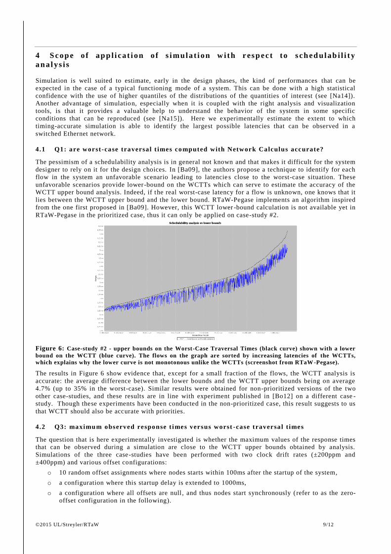
Figure 6: Case-study #2 - upper bounds on the Worst-Case Traversal Times (black curve) shown with a lower

bound on the WCTT (blue curve). The flows on the graph are sorted by increasing latencies of the WCTTs,

which explains why the lower curve is not monotonous unlike the WCTTs (screenshot from RTaW -Pegase).

The results in Figure 6 show evidence that, except for a small fraction of the flows, the WCTT analysis is

accurate: the average difference between the lower bounds and the WCTT upper bounds being on average

4.7% (up to 35% in the worst-case). Similar results were obtained for non-prioritized versions of the two

other case-studies, and these results are in line with experiment published in [Bo12] on a different case -

study. Though these experiments have been conducted in the non-prioritized case, this result suggests to us

that WCTT should also be accurate with priorities.

4.2 Q3: maximum observed response t imes versus worst -case traversa l t imes

The question that is here experimentally investigated is whether the maximum values of the response times

that can be observed during a simulation are close to the WCTT upper bounds obtained by analysis.

Simulations of the three case-studies have been performed with two clock drift rates (±200ppm and

±400ppm) and various offset configurations:

o 10 random offset assignments where nodes starts within 100ms after the startup of the system,

o a configuration where this startup delay is extended to 1000ms,

o a configuration where all offsets are null , and thus nodes start synchronously ( refer to as the zero-

offset configuration in the following).

©2015 UL/Streyler/RTaW 10/12

Results discussed here have been obtained with a simulation time set to 8 days of functioning time, The

same experiments performed with 2 days of simulation lead to the same results for the two larger case-

studies while for case-study #1 simulating 8 days instead of 2 days allowed to decrease the difference with

WCTT by 3% both for the average and max value. Whatever the case-study, what we observe is that no

random offset assignments lead to significantly different results than the others. For instance, in case-study

#1 the average difference for the maximum latency is 6.3% among 10 simulations with distinct random

assignments of 2 days. Larger offset intervals and clock drift rates did not make a difference either in our

experiments.

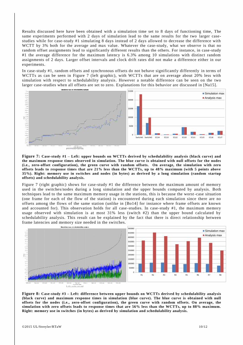
In case-study #1, random offsets and synchronous offsets do not behave significantly differently in terms of

WCTTs as can be seen in Figure 7 (left graphic), with WCTTs that are on average about 20% less with

simulation with respect to schedulability analysis . However a notable difference can be seen on the two

larger case-studies when all offsets are set to zero. Explanations for this behavior are discussed in [Na15].

Figure 7: Case-study #1 – Left: upper bounds on WCTTs derived by schedulability analysis (black curve) and

the maximum response times observed in simulation. The blue cur ve is obtained with null offsets for the nodes

(i.e., zero-offset configuration), the green curve with random offsets. On average, the simulation with zero

offsets leads to response times that are 21% less than the WCTTs, up to 48% maximum (with 5 points above

35%). Right: memory use in switches and nodes (in bytes) as derived by a long simulation (random startup

offsets) and schedulability analysis.

Figure 7 (right graphic) shows for case-study #1 the difference between the maximum amount of memory

used in the switches/nodes during a long simulation and the upper bounds computed by analysis. Both

techniques lead to the same maximum memory usage in the stations, this is because the worst -case situation

(one frame for each of the flow of the station) is encountered durin g each simulation since there are no

offsets among the flows of the same station (unlike in [Bo14] for instance where frame offsets are known

and accounted for). This observation holds for all case -studies. In case-study #1, the maximum memory

usage observed with simulation is at most 31% less (switch #2) than the upper bound calculated by

schedulability analysis. This result can be explained by the fact that there is direct relationship between

frame latencies and memory size needed in the swi tches.

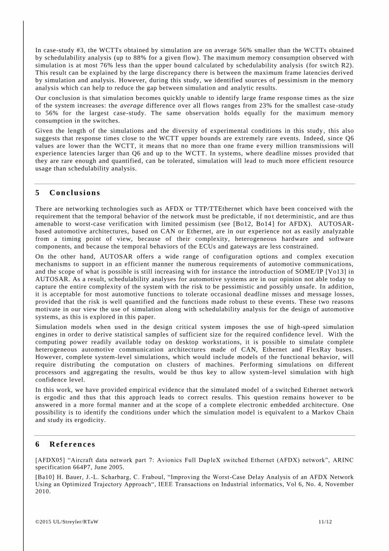
Figure 8: Case-study #3 – Left: difference between upper bounds on WCTTs derived by schedulability analysis

(black curve) and maximum response times in simulation (blue curve). The blue curve is obtained with null

offsets for the nodes (i.e., zero-offset configuration), the green curve with random offsets. On average, the

simulation with zero offsets leads to response times that are 56% less than the WCTTs, up to 88% maximum.

Right: memory use in switches (in bytes) as derived by simulation and schedulability analysis.

0

5000

10000

15000

20000

25000

Switch#1 Switch#2 ECU4 ECU3 ECU2 ECU0 ECU1 ECU5 ECU6 ECU7

Simulation max

Analysis max

0

50000

100000

150000

200000

250000

300000

350000

400000

450000

500000

R1 R2 R3 R4 R5 R6 R7 R8

Simulation max

Analysis max

©2015 UL/Streyler/RTaW 11/12

In case-study #3, the WCTTs obtained by simulation are on average 56% smaller than the WCTTs obtained

by schedulability analysis (up to 88% for a given flow). The maximum memory consumption observed with

simulation is at most 76% less than the upper bound calculated by schedulability analysis (for switch R2).

This result can be explained by the large discrepancy there is between the maximum frame latencies derived

by simulation and analysis. However, during this study, we identified sources of pessimism in the memory

analysis which can help to reduce the gap between simulation and analytic results.

Our conclusion is that simulation becomes quickly unable to identify large frame response times as the size

of the system increases: the average difference over all flows ranges from 23% for the smallest case-study

to 56% for the largest case-study. The same observation holds equally for the maximum memory

consumption in the switches.

Given the length of the simulations and the diversity of experimental conditions in this study , this also

suggests that response times close to the WCTT upper bounds are extremely rare events. Indeed, since Q6

values are lower than the WCTT, it means that no more than one frame e very million transmissions will

experience latencies larger than Q6 and up to the WCTT. In systems, where deadline misses provided that

they are rare enough and quantified, can be tolerated, simulation will lead to much more efficient resource

usage than schedulability analysis.

5 C on c lus i ons

There are networking technologies such as AFDX or TTP/TTEthernet which have been conceived with the

requirement that the temporal behavior of the network must be predictable, if no t deterministic, and are thus

amenable to worst-case verification with limited pessimism (see [Bo12, Bo14] for AFDX). AUTOSAR-

based automotive architectures, based on CAN or Ethernet, are in our experience not as easily analyzable

from a timing point of view, because of their complexity, heterogeneous hardware and software

components, and because the temporal behaviors of the ECUs and gateways are less constrained.

On the other hand, AUTOSAR offers a wide range of configuration options and complex execution

mechanisms to support in an efficient manner the numerous requirements of automotive communications,

and the scope of what is possible is still increasing with for instance the introduction of SOME/IP [Vo13] in

AUTOSAR. As a result, schedulability analyses for automotive systems are in our opinion not able today to

capture the entire complexity of the system with the risk to be pessimistic and possibly unsafe. In addition,

it is acceptable for most automotive functions to tolerate occasional deadline misses and message losses,

provided that the risk is well quantified and the functions made robust to these events. These two reasons

motivate in our view the use of simulation along with schedulability analysis for the design of automotive

systems, as this is explored in this paper.

Simulation models when used in the design critical system imposes the use of high-speed simulation

engines in order to derive statistical samples of sufficient size for the required confidence level. With the

computing power readily available today on desktop workstations, it is possible to simulate complete

heterogeneous automotive communication architectures made of CAN, Ethernet and FlexRay buses.

However, complete system-level simulations, which would include models of the functional behavior, will

require distributing the computation on clusters of machines. Performing simulations on different

processors and aggregating the results, would be thus key to allow system-level simulation with high

confidence level.

In this work, we have provided empirical evidence that the simulated model of a switched Ethernet network

is ergodic and thus that this approach leads to correct results. This question remains however to be

answered in a more formal manner and at the scope of a complete electronic embedded architecture. One

possibility is to identify the conditions under which the simulation model is equivalent to a Markov Chain

and study its ergodicity.

6 R ef eren ces

[AFDX05] “Aircraft data network part 7: Avionics Full Dup leX switched Ethernet (AFDX) network”, ARINC

specification 664P7, June 2005.

[Ba10] H. Bauer, J.-L. Scharbarg, C. Fraboul, “Improving the Worst -Case Delay Analysis of an AFDX Network

Using an Optimized Trajectory Approach“, IEEE Transactions on Industrial informatics, Vol 6, No. 4, November

2010.

©2015 UL/Streyler/RTaW 12/12

[BoTh07] A. Bouillard and E. Thierry, “An algorithmic toolbox for network calculus”, Discrete Event Dynamic

Systems, 17(4), october 2007.

[Bo11] M. Boyer, J. Migge, and M. Fumey, “PEGASE – a robust and efficient tool for worst-case network

traversal time evaluation on AFDX”, SAE Aerotech 2011, Toulouse, France, 2011.

[Bo11b] M. Boyer, J. Migge, N. Navet, “A simple and efficient class of functions to model arrival curve of

packetised flows“, First International Workshop on Worst-case Traversal Time (WCTT), in conjunction with the

32nd IEEE Real-time Systems Symposium (RTSS), Vienna, Austria, November 29, 2011.

[Bo12] M. Boyer, N. Navet, M. Fumey, “Experimental assessment of timing verification techniques for AFDX“,

Embedded Real-Time Software and Systems (ERTS 2012), Toulouse, France, February 1 -3, 2012.

[Bo14] M. Boyer, L. Santinelli, N. Navet, J. Migge, M. Fumey, “ Integrating end-system frame scheduling for

more accurate AFDX timing analysis“, Embedded Real-Time Software and Systems (ERTS 2014), Toulouse,

France, February 5-7, 2014.

[Bo14b] M. Boyer, L. Fejoz, S. Merz, “Proof-by-Instance for Embedded Network Design: From Prototype to

Tool Roadmap“, Embedded Real-Time Software and Systems (ERTS 2014), Toulouse, France, February 5 -7,

2014.

[CL15] M. Claypool, “Modeling and Performance Evaluation o f Network and Computer Systems - Simulation”,

Course CS533, Worcester Polytechnic Institute, 2015.

[Da07] R. Davis, A. Burn, R. Bril, and J. Lukkien, “Controller Area Network (CAN) schedulability analysis:

refuted, revisited and revised”, Real-Time Systems, vol. 35, pp. 239–272, 2007.

[Da12] R. Davis, N. Navet, "Controller Area Network (CAN) Schedulability Analysis for Messages with

Arbitrary Deadlines in FIFO and Work-Conserving Queue", 9th IEEE International Workshop on Factory

Communication System (WFCS 2012), Lemgo/Detmold, Germany, May 21 -24, 2012.

[It07] J.B. Itier, “A380 Integrated Modular Avionics”, ARTIST2 meeting on Integrated Modular Avionics, 2007.

[Ma13] E. Mabille, M. Boyer, L. Fejoz, and S. Merz, “Certifying Network Calculus in a Proof Assistant”, 5th

European Conference for Aeronautics and Space Sciences (EUCASS), Munich, Germany, 2013.

[Ma13b] C. Mauclair, “Une approche statistique des réseaux temps réel embarqués”, Phd thesis from the

University of Toulouse, 2013.

[Mo12] A. Monot, N. Navet, B. Bavoux, "Fine-grained Simulation in the Design of Automotive Communication

Systems", Embedded Real-Time Software and Systems (ERTS 2012), Toulouse, France, February 1-3, 2012.

[Na14] N. Navet, S. Louvart, J. Villanueva, S. Campoy-Martinez, J. Migge, “Timing verification of automotive

communication architectures using quantile estimation“, Embedded Real-Time Software and Systems (ERTS

2014), Toulouse, France, February 5-7, 2014.

[Na15] N. Navet, J. Seyler, J. Migge, "Timing verification of real -time automotive Ethernet networks: what can

we expect from simulation?", technical report of the University of Luxembourg, to appear in 2015.

[Na11] N. Navet, A. Monot, B. Bavoux, " Impact of clock drifts on CAN frame response time distributions", 16th

IEEE International Conference on Emerging Technologies and Factory Automation (ETFA 2011), Industry

Practice track, Toulouse, September 2011.

[Se13] J. Seyler, "A Tool-Chain for Modeling and Evaluation of Automotive Ethernet Networks", Autom otive

Bus systems + Ethernet, Stuttgart, Germany, December 9-11, 2013.

[Se15] J. Seyler, T. Streichert, M. Glaß, N. Navet, J. Teich, “Formal Analysis of the Startup Delay of SOME/IP

Service Discovery”, DATE 2015, Grenoble, France, March 9 -13, 2015.

[Se15b] J. Seyler, N. Navet, L. Fejoz, “Insights on the Configuration and Performances of SOME/IP Service

Discovery“, SAE World Congress, Detroit, USA, April 21 -23, 2015.

[SoAd] AUTOSAR, “Specification of Socket Adaptor”, Release 4.2.1, 2015. Available at url

http://www.autosar.org/.

[Vo13] L. Völker, “SOME/IP – Die Middleware für Ethernet-basierte Kommunikation”, Hanser automotive

networks, 2013.

[Ze09] H. Zeng, M. D. Natale, P. Giusto, and A. L. Sangiovanni-Vincentelli, “Stochastic Analysis of CAN-Based

Real-time Automotive Systems,” IEEE Trans. Industrial Informatics, vol. 5, no. 4, pp.388 –401, 2009.

[Ze10] H. Zeng, M. D. Natale, P. Giusto, and A. L. Sangiovanni -Vincentelli, “Using statistical methods to

compute the probability distribution of message response time in Controller Area Network,” IEEE Trans.

Industrial Informatics, vol. 5, no. 4, pp.678–691, 2010.