TIME • FREQUENCY SIGNAL...

Published in Australia, New Zealand, the Pacific, Asia and Africa by Longman Cheshire Pty Limited Longman House Kings Gardens 95 Coventry Street Melbourne 3205 Australia ISBN 0 582 71286 6

Offices in Sydney, Brisbane, Adelaide and Perth. Associated companies, branches and representatives throughout the world.

Copublished in the Western Hemisphere, United Kingdom and Europe by Halsted Press: an Imprint of John Wiley & Sons, Inc. New York Toronto Chichester

Copyright e Longman Cheshire 1992 First published 1992

All rights reserved. Except under the conditions described in the Copyright Act 1968 of Australia and subsequent amendments, no part of this publication may be reproduced, stored in a retrieval system or transmitted in any form or by any means, electronic, mechanical, photocopying, recording or otherwise, without the prior permission of the copyright owner.

Designed by Nadia Graziotto Printed in Hong Kong

National Library of Australia Catalogulng-lu-PubUcation data

Time-frequency signal analysis. Bibliography. Includbs index. ISBN 0-582-71286-6 l.Signal processing. I. Boashash, Boualem. 621. 3$223

Library of Congress Cataloguing-ln-PubUcation data

Time-frequency signal analysis-methods and applications/edited by Boualem Boashash. p. cu. Includes bibliographical references and index. ISBN 0-470-21821-5 1. Signal processing. I. Boashash, Boualem. YK5102.T585 1992 621.382'2-dc20 91-32658

CIP

TIME • FREQUENCY SIGNAL ANALYSIS METHODS AND APPLICATIONS

Edited by Boualem Boashash

~.~ ••• • •• Longman Cheshire

Chapter 12

Signal Detection Using Time-Frequency Analysis

Boualem Boashash and Peter O'Shea

Keywords: detection, time-frequency, Wigner-Ville distribution, cross Wigner-Ville distribution, pattern recognition, time-varying higher order spectra, multilinear

1 Introduction: The need for time-frequency detectors

The detection of known signals in white Gaussian noise is a comparatively well understood and well documented problem [1]. Its solution is often expressed in terms of time domain correlations. These time domain expressions can be implemented very efficiently, and for this reason are widely used. In many practical situations, however, the signal to be detected is not known, and at best some a priori information about it is available. In such cases, the classical time domain solutions become limited ... These limitations have prompted solutions to the detection problem in terms of time-frequency distributions (TFDs). There are a large number of these TFDs [see chapter 1], each with their own particular features, and as a consequence, great potential exists for detection of signals with various forms of a priori knowledge. In the case where the true signal is known precisely, one can obtain time-frequency (t-f) domain solutions exactly equivalent to many of the conventional time domain detection methods. That is, matched filtering may be implemented via t-f correlations, energy detection may be implemented via an integration of the t-f representation over time and frequency, etc. Additional flexibility exists however, with the t-f domain solutions for the cases of imprecisely known signals, or where

280 Time-Frequency Signal Analysis

particular features only of the signal are important. Time-varying filtering may be incorporated into the matched filtering process, for example, so as to emphasise certain regions of the t-f plane [2]; energy detection may be performed over specific t-f regions [3]; the presence of time-varying frequency lines can also be tested [see chapter by Barrett and Streit].

Although an infinite number of TFDs of the so-called Cohen's class [see chapter 1] are possible tools for detection, some have attained greater popularity than others. The spectrogram has long been used for the purposes of detection and estimation [4]. For quasi-stationary signals it provides a good environment for frequency estimation, line tracking and detection [see chapter by Barrett and Streit], and detection of signals subject to random Doppler or time shifts [4]. The Wigner-Ville distribution (WVD) has been proposed for detection schemes in several different applications [5], [6], [7]. Its popularity is largely due to the fact that it provides good time-frequency localisation for signals such as chirps, and is an energy preserving transform [8]. Another representation which has been proposed for detection is the wavelet transform [9]. This is an affine representation which yields a frequency resolution which is dependent on frequency.

In this chapter, emphasis will be placed on detection methods involving the Wigner-Ville distribution. This representation has been chosen for many reasons which will be illustrated in the applications presented.

2 Review of detection and classification methods

2.1 Detection

The problem of detecting and classifying transients of unknown waveshape is becoming increasingly important, particularly in surveillance environments. The detection problem amounts to trying to determine whether or not a signal, s( t), is present in a noisy environment. For white Gaussian noise, n(t), with an observed signal given by r(t), the problem can be modeled as:

r(t) = n(t) r(t) = s(t) + n(t)

(1)

Signal Detection Using Time-Frequency Analysis 281

Hl 11- > .,- <

Ho

(2)

where Hl is the hypothesis that the signal is present, Ho is the hypothesis that the signal is not present, and "1 is the detection statistic which must be compared with a threshold, l.

A number of detectors have been proposed for the detection problem. The earliest and perhaps simplest were the energy detector, and the spectral density correlator. The energy detector, although very simple performs quite well for signals of any waveshape, and for this reason is very widely used. It is not, however, optimal. The optimal detector may be implemented by obtaining a minimum variance estimate of the true signal and using this in a conventional detector. Various means have appeared in the recent literature for performing the estimation stage of this type of 'adaptive' detector.

One technique is documented in [10]. The authors in [10] proposed that the signal, s(t), be estimated as the impulse response of a filter having a rational system function, H(z), with the unknown parameter vector being determined using a modified maximum likelihood estimator. It is shown in [10] that this estimator is approximately distributed as the ratio of quadratic forms: under Ho the distribution is central, while under H 1 , it is non-central with a bias term. The authors then showed that this adaptive detector performs better than the energy detector, at least when the noise variance is known, and when the number of parameters to be estimated is small compared with the number of data points (the performance was 'better' in the sense of having higher detection probability for a given false alarm probability) [10].

Another approach to the estimation stage of the adaptive detector is to enhance the signal by a combination of out of band conventional filtering and in band filtering using eigenanalysis [11].

Bispectrum analysis is yet another technique which has been used for transient enhancement [12]. The rationale used here is that if the probability distribution function (pdf) of the noise is non-skewed, then the noise contribution in the third order cumulant (bispectrum) will be zero. The class of data for which the technique may be used is that for which the third order cumulant of the noise free signal is non-zero. The authors in [12] presented a method of reconstruction based on a modelling of the signal as the impulse response of an AR process, with a subsequent minimisation of the third order cumulant. Simulations were provided to show that for the particular data considered, the bias and variance of the reconstructed signals was lower than for the methods of Kumaresan and Tufts [13]' or minimum mean-square error estimates [1].


While adaptive detection works well for a number of signals, there will still be many situations, where due to the complex nature of the signal waveshape,it is impractical to implement. One may, in these cases, generalise the concepts of energy or ,spectral density correlators to obtain improved performance. One can modify the energy detector, for example, by using higher order cumulants, rather than simply the second order one. Both the third and fourth order cumulants are zero for Gaussian processes, and exhibit superposition for independent random variables. Thus these cumulants provide a means for discriminating non-Gaussian signals from Gaussian noise. Alternatively, the cumulant spectra may be used for performing the discrimination [14]. This is a useful prospect for the underwater environment where the noise is very close to Gaussian. It must be noted, however, that for these detectors to work well, reliable estimates of the cumulants must be obtained. Consequently a large number of data samples is needed.

In a similar vein, for short duration signals, one may generalise the spectral density correlator by using the wavelet transform to perform the spectral estimation rather than a conventional Fourier transform. The wavelet transform uses low BT (bandwidth-time) wavelets as its basis functions, rather than the infinite sines and cosines of the Fourier transform. It consequently has high time resolution for high frequencies and is able to detect sharp edges well. See for example, figures 12.1 and 12.2 which show respectively the spectrogram and the wavelet transform for a rectangular pulse. Much more concentrated spikes appear at the pulse edges for the wavelet transform due to the better time resolution.

A further possibility for detection is to use a count of the number of zero-crossings as the detection statistic [15]. This type of detection will be ineffective for certain 'noise-like' signal shapes, but is still useful for a large class of signals.

2.2 Classification Where classification is required in addition to detection, one needs to determine the beginning and end of the transient. For moderate to high signal to noise ratio (SNR) one can use AR based segmentation algorithms [16]. For low SNR one may need to use an energy detector or a cumulant based detector. Once the transient has been isolated in time, several different classification procedures are possible. High order AR parameters were used as features for a classification procedure in [17], which is based on a minimisation of the distance between the unknown transient and anyone of a set of known ones. Recently, advances have been made on classification reliability by using schemes involving neural networks [see chapter by Malkoff], Hidden Markov models [18]' and a dynamic time warping approach [19].


Pulse stft

229731

153154

765770

000000

Figure 12.1. Spectrogram of a rectangular pulse.

3 Signal detection using the WVD

3.1 Theory of Wigner-Ville and cross Wigner-' Ville based detection

Many of the detection methods outlined in section 2 work well in a number of circumstances. However, where the transients are non-stationary or where the arrival times are unknown, a different approach is often appropriate. Many authors have proposed detection schemes involving TFDs, such as the spectrogram [4], the WVD [5], [6], [7], and the wavelet transform [9]. These TFDs all have their advantages, but one, the WVD will be considered in detail here. This is because it is a real energy preserving transform, and because it provides high resolution in time and frequency for chirp type signals. Its properties are outlined in chapter 1. The WVD and cross WignerVille distribution (XWVD) are defined respectively by:


Pulse wave 1

1 13457

756380

378190

000000

Figure 12.2. Wavelet transform of a rectangular pulse.

(3)

(4)

where zs(t) is the analytic signal corresponding to s(t) and zr(t) is the analytic signal corresponding to r(t) [20].

An important equation in the theory of WVD detection is Moyal's formula [8] which states that for any analytic signals, Zl(t), Z2(t), Z3(t) and Z4(t), the following relationship holds:

(5)


This equation shows that there is an equivalence between time domain correlations and XWVD correlations. The time domain correlations which appear as the solutions to many classical detection problems, then, may be replaced by equivalent WVD (XWVD) correlations [21]. In fact the relationship between correlations and XWVDs extends further than Moyal's formula suggests. One can show that the Wigner-Ville spectrum (which is simply the expected value of the Wigner-Ville distribution) is the Fourier transform of the autocorrelation function [22]. Similarly the XWVD is the 2D Fourier transform of the cross-correlation function [see chapter by Boles and Boashash]. We are led naturally, then, to substitute the WVD for the autocorrelation function, and the XWVD for the cross-correlation function in detectors and estimators for non-stationary processes. The advantage of this replacement is that time-frequency feature isolation and consequent noise suppression using time-varying filtering can then be easier [3], especially where the signal waveshape is unknown.

Consider a signal, s(t), with energy A, which is sent through a noisy transmission channel, so that the output of the channel is r(t) = s(t) + n(t), where n(t) is a zero mean, white Gaussian noise process of variance, No. The classical solution to the detection problem for a known signal is the matched filter, its detection statistic being given by:

(6)

where < ZrZs > denotes the inner product of zr(t) and zs(t), as defined by (6), and

SNR= lA/No (7)

Here the SNR is defined as the difference in means under the two hypotheses, given unit average variance [6], and is expressed as:

SNR = IECf/IHd - E(ryIHo)I/{1/2[var(ryIHd + var(ryIHo)]}I/2 (8)

where E(ryIHo) and E(rylHd are the expected values of ry under Ho and HI respectively, while var(ryIHo) and var(ryIHI) are the variances under Ho and HI'

In [6],Kumar and Carroll proposed a WVD based detection scheme and a XWVD based detection scheme, their detection statistics being given respectively by:

and

) +00 r+oo rywvd = -00 .!-OO WZr(t, f)Wz,(t, f)dtdf

[+00 t+oo T'xwvd = I I

.J-oo .I~OO

(t, f) VVzs f)dtdf

(9)

(10)


By Moyal's formula the WVD based detection statistic can be shown to be equivalent to a squared correlation function. That is

(11)

This detection statistic will then be suboptimal for a precisely known signal, but has application in the detection of signals with random amplitude functions (Raleigh fading signals), where the statistic in (11) is optimal [7J. The SNR of this detection statistic was derived in [6J and is given by

SNR = j A/No .1/\/1 + No/A (12)

At high SNR it approaches the matched filter detection statistic, but degrades at low SNR: '''One may also obtaine$f a simplified expressipn for the XWVD based detection statistic using Moyal's formula:

'Tlxwvd =< ZrZs >< ZsZs >= A < ZrZs > (13)

The XWVD detection statistic is thus the matched filter detection statistic multiplied by the signal energy (i.e. by a constant). Hence, the SNR for XWVD detection will be identical to that of the matched filter. The XWVD detection statistic may then be used as a replacement for the conventional matched filter in any application. Its advantage over the matched filter is that one may perform pre- and post-processing of the t-f representations involved, according to any a priori information that may be available.

3.2 Practical application of the WVD and XWVD based schemes

,Detection, estimation and classification via Wigner-Ville spectra For non-stationary signals the time-varying power spectral density may be shown to be the expected value of the Wigner-Ville distribution [22J:

S(t,f)= E{ ~ R(t,T)}=E{ ~ [zs(t+T/2)z;(t-T/2)]} (14)

E{Wzs(t, I)}

where :F denotes Fourier transform in the T variable. If an ensemble T

of realisations is available, then, the WVDs from the ensemble may be


averaged, and time-varying spectra are obtained. The cross-terms of the TFD are smoothed out by the ensemble averaging. The resulting spectra may be used to obtain various time-frequency features in a way which is not available from the time domain signals. Time averaging may also be used to yield estimates, if some condition of local ergodicity is verified.

A practical example illustrating the usefulness of WVD based spectra is found in magnetotelluric prospecting [23J. Broadband magnetotelluric energy is trapped in the earth ionosphere waveguide, so that field strength measurements at the earth's surface may be used to measure the resistivity of the earth as a function of frequency, and hence depth below the receiving site. The technique relies on calculating complex impedance as the ratio of electric and magnetic fields. The electric allci.llH1gnetic fields may be combined in four different ways, and so an ensemble of four measurements is possible. Normally the electric and magnetic field measurements are first Fourier transformed so as to provide a frequency dependent impedance profile, but these Fourier based techniques are limited, due to a number of factors. Firstly, the magnetotelluric signals have significant non-stationary spectral content which is smeared in the PSD. Secondly there is a log-normal distribution of the impedance as a function of frequency which can not easily be accounted for by the inherently linear averaging of the Fourier transform. It has been found that significantly better performance results by obtaining the impedance measurements via WVDs. The WVD based procedure involves dividing the electric and magnetic field derived WVD matrices to yield a time evolving estimate of the impedance vs frequency. The time estimates are then averaged logarithmically according to the expected distribution of the impedance values. The resulting reduction in bias over that obtained with Fourier techniques is about eightfold [23J.

Pattern recognition Often what is required in a detection environment is not to detect an exactly known signal, but to detect a pattern in frequency or time-frequency. WVD patterns spaces have been found useful in a number of practical applications. In the chapter by Forrester, WVD patterns are seen to be useful for detecting helicopter gear faults. In [24J they were used for the detection of heart abnormalities in electrocardiograph (EeG) signals, with the shape of the WVD's crossterms being found to be effective for detecting the presence of a particular unhealthy heart condition. In section 4 of this chapter WVD patterns are seen to be useful in classifying underwater signals pertaining to rotating machinery.

Time-frequency feature extraction For detection, estimation and classification problems which involve


particular frequency features, the frequency domain is often used in preference to the time domain. For detecting and estimating sinusoidal tones, for example, the PSD is often used. Where a certain frequency signature is available, the PSD is also commonly used. However, where the signals under analysis are non-stationary, frequency domain based feature isolation becomes inadequate and time-frequency representations must be used. These representations include the spectrogram, the ambiguity function, the WVD, the XWVD, the ZAM distribution [25] etc. Each of them has its own particular characteristics which may be desirable in a given application. A brief outline of the advantages of each is provided below.

The spectrogram is a widely used TFD which provides very good time-frequency characterisation for quasi-stationaq, "or. 'slowly varying signals. A good description of its properties may be found in [4].

The WVD and XWVD are other representations which characterise the time-varying frequency content of a signal by exhibiting an energy concentration along the frequency laws of the signal components [3]. It is this energy concentration property which allows for good frequency law estimation, tracking and detection. At moderate to high SNR Rao and Taylor have shown the WVD to be optimal for detecting linear frequency laws J26l, while the XWVD may be used for frequency law estimation at lower SNRs [26]. In the case of multicomponent signals, the presence of cross-terms between true signal components can yield a visually confusing representation [3]. The representation may still be useful in practice, though, since a tracking algorithm may be applied to enhance frequency law estimates, and the highly oscillatory cross-terms may be "invisible" to these trackers [27]. An application of WVD based feature detection is provided in the section 3.3.

The ZAM distribution is another recently developed t-f representation which has good t-f energy concentration along with minimal cross-terms [25]. These two properties make it a useful prospect for detection and classification purposes.

Detection of signals subject to delay and Doppler The ambiguity function defined in (15) is used to detect signals subject to a Doppler and time shift:

(15)

The WVD and XWVD have a similar ability to detect time and Doppler shifted signals, a fact which is not surprising since they are related to the auto and cross ambiguity functions by 2D Fourier transformation. The chapter by Boles and Boashash gives an example of the use of the XWVD in the seismic context for detecting signals


subjected to time shifts. These time shifts arise from signals which are reflected from the different underground strata, and hence provide information as to the nature of the subterranean surface.

3.3 Example of WVD based feature extraction

As already mentioned, the WVD and XWVD based schemes have potential for a variety of pre and post-processing operations. One of the useful properties of the WVD is its ability to localise energy about the instantaneous frequency (IF) law of the of the signal. This property is exploited in the example presented here.

In detecting unknown signals, it is necessary to first estimate the signal, or equivalently its TFD. Suppose the signal to be detected is a randomly jittering frequency modulated signal, zsCt);UrikilOwn complex amplitude, unknown frequency law and random uniformly distributed phase. If the IF can be estimated, a signal estimate may be formed by:

Zs(t) = AIIT(t - T/2)e j27r4>(t) (16)

t -where 1>(t) = .fa f(a)da, for IIT(t) = 1, -T/2 ::; t ::; T/2 and 0 elsewhere, and A2 is the estimate of the amplitude.

The IF law of this signal estimate will actually differ from the true law by the IF jitter. Thus the signal may be modeled as a signal of random complex amplitude whose frequency at any point in time is randomly jittered by the uncertainty in the IF and amplitude. The IF estimation may be achieved by use of ML techniques [26]. Denoting the time-varying pdf of the IF error as p(t, f), then the expected value of the WVD of the true signal is determined after [21] as:

(17)

where WZs (t, 1) is the WVD of the signal estimate. The optimal detection statistic for a signal of random Rayleigh distributed amplitude is known to be given by a correlation of the WVDs of the true and observed signals. Thus, the required detection statistic is:

(18)

It is seen that the optimal detector can be implemented by correlating the observed WVD with a smeared version of the WVD of the signal estimate. This smeared WVD is in fact a windowed WVD, in which the effective window [28] is of the form of the inverse Fourier transform of the of the IF could a.lso recover it

t

"


signal estimate from this WVD estimate using t-f synthesis techniques if required (see chapter 17).

Simulations were performed to adaptively detect I;t signal with linear IF law using the method outlined above. The signal was a short linearly frequency modulated signal with the following parameters: duration -0.128 secs., sampling freq-1kHz, frequency lwa -O.lkHz to 0.4 kHz. The juttering in the signal was preset to give a jittering bandwidth of O.025kHz for all values of time. The jitter was Gaussian. Figure 12.3 compares the performance with the classical energy detector. The WVD based scheme performs better than the energy detector, indicating its potential for time-varying signal detection.

3.4 Application of higher order statistics to time,:: frequency analysis '.' .

There has been a great deal of interest in recent years in the use of higher order statistics. These statistics use more information than is available simply from the mean and variance of a process, and hence provide better discrimination in some applications. One area where these statistics have found application is in detection. Dwyer [29], for example, has proposed use of a frequency domain kurtosis measure (i.e. a normalised fourth order frequency moment) rather than the usual second order frequency moments (i.e. the PSD) to enhance detection probability for certain signals. Hinich has proposed the bispectrum for detection in [14]. A third order spectrum for non-stationary signals, which could conceivably be used for detection, has also been proposed by Gerr [30]:

(19)

This is not the only possible extension of the Wigner distribution to higher order spectra, however. One possible alternative is to simply take the bispectrum of the WVD's bilinear kernel:

(20)

where B is the bispectrum operator on the r variable, and K(t, r) is the bilinear WVD kernel, given by

(21)

't'!-¥

0

" * " >. e> '" c: w

0 0 0 0 0 C! (J) <Xl I"- <0

0 0 0 0


'" C\i

9 ... 0 "t til .., til ~

~ til ::: til ~

§ til

t=:: ~ ..::: 0 <>

a: C! UJ

~ Z 0 til ff> "

UJ 0:1 ., ..0 e;-

~ .. .s til C)

::: 0:1

@ '@

o

til p.,

::: 0 :g til

"tl Ci

M C'i .... til I-<

'" 0 0 0 0 0 0

~ '" .... CO) '" C! 0 0 0 0 0 0

Al!l!QeqoJd UO!pS1Sa


This representation would retain the resolution enhancement properties of the WVD, and would have a number of useful properties associated with higher order spectra. It is also likely to have reduced cross-terms as compared with Gerr's formulation.

Yet another means of extending the Wigner-Ville distribution to higher orders is through the use of generalised WigneT- Ville distTibutions. These representations give much better energy concentration for non-linear FM signals than does the conventional WVD. Further, for random signals they have an important interpretation as time-vaTying higheT oTdeT spectra. The details of these functions are provided in the appendix.

A further application of higher order statistics to time-frequency analysis lies in the use of the fourth order spectrum for time-varying frequency estimation. The fourth order cumulant is generally a function of three time delays, but a special form may be defined, in which there is only one delay [31]. A useful property of this cumulant is that its spectrum, for a Gaussianly amplitude modulated sinusoid, tends to a delta function. This is so even for a sinusoid modulated by white noise, whereas the conventional PSD is fiat. Thus frequency or instantaneous frequency estimation of certain wide band processes may be implemented with fourth order rather than second order spectral estimators.

3.5 Digital implementation

The theory of WVD and XWVD based detection carries over in a straightforward manner from continuous to discrete time. One only needs to ensure that the analytic signal is used to avoid aliasing [2], [32]. The discrete XWVD is defined as:

+L pX lx3(n,k) =2 2...:: xl(n+l)x;(n_l)e-j47rkl/N (22)

l=-L

where Xl(t) and X3(t) are time-limited to (-T/2,T/2), T is even and nand k are the discrete time and frequency variables respectively, and N = T + 1. A rectangular window is used, so that L = T /2 -Inl. The inner product of 2 discrete XWD's is correspondingly defined by [6]:

+T/2 N-l

rj = 2...:: 2...:: pX1X3(n,k)p~2X4(n,k) (23) n=-T/2 k=O

Further details relating to the discrete implementation may .be found in [28] and in the chapter by Boashash and Reilly.


4 Applications

4.1 Time-frequency signaturing

Signaturing of engine firing signals with the WVD This section presents an application of WVD and XWVD based techniques to time-frequency signaturing. The signals chosen for signaturing are the individual firings of an engine. The aim is to test the effectiveness of the signaturing by seeing whether it is possible to classify a given firing according to the cylinder which produced it. To perform the classification it was necessary to first segment the engine noise according to its firings. A four step procedure which was developed for this purpose appeared in [33] and is summarised below.

'Step 1: Estimation of the engine jiTing rate and the numbeT of cylindeTs

This step is required to segment the engine signal into individual cylinder firings. In the process of performing this segmentation it is necessary to determine the engine firing rate (EFR), as well as the number of cylinders. The method used for determining them is based on the autocorrelation function (ACF). Important operating engine characteristics are given by the crankshaft rotation rate or engine speed (CSR.), and the firing rate of a particular cylinder (CFR). The following relationships hold for a four stroke engine:

CFR = CSR/2 and EFR = CFR x Number of Cylinders (24)

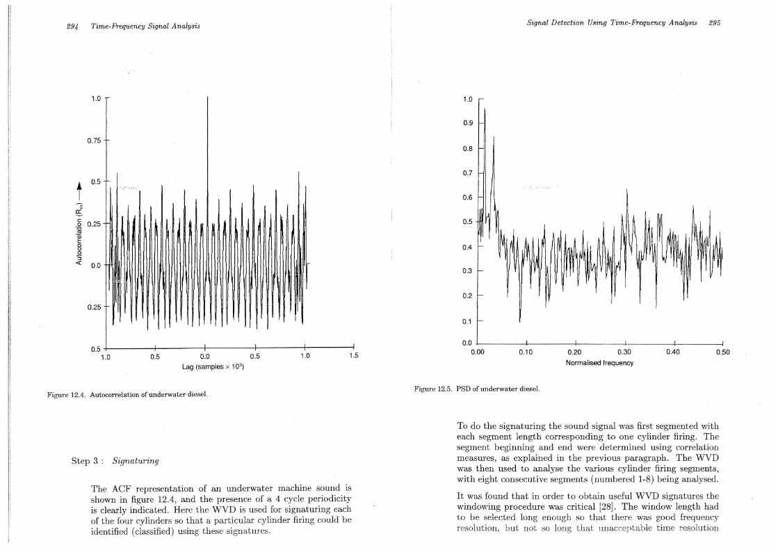
The autocorrelation can often show up periodicities in a way which is easier to interpret than the PSD, as can be seen from figures 12.4 and 12.5. Figure 12.4 displays a much more obvious 4 cycle periodicity than figure 12.5. The autocorrelation functioll, then, can provide a more informative representation of short term periodicities, and is thus preferred over the PSD in this application.

Step 2: Detection

For classification to be successfully performed it is necessary to localise accurately in time the occurrence of an event. That is, accurate detection must be performed. To perform this detection the ACF was again found to be a very useful tool. One can see clearly in figure 12.4 that cylinder firing events are detected quite easily by correlation techniques (by noting when a specified threshold is exceeded). The reference time for a specific event occurring was therefore taken as the time of local maximum correlation.

2g4 Time-Frequency Signal Analysis

1.0

0.75

t 0.5

~ c:

0.25 0 .~

~ 15 C)

.8 ::l

<C 0.0

0.25

0.5+---------+---------~--------~-------4---------

1.0 0.5 0.0 0.5 1.0 1.5

Lag (samples x 103)

Figure 12.4. Autocorrelation of underwater diesel.

Step 3: Signaturing

The ACF representation of an underwater machine sound is shown in figure 12.4, and the presence of a 4 cycle periodicity is clearly indicated. Here the WVD is used for signaturing each of the four cylinders so that a particular cylinder firing could be identified (classified) using these signatures.

1.0

0.9

0.8

0.7

0.6

0.5

0.4

0.3

0.2

0.1

0.0 0.00


0.10 0.20 0.30

Normalised frequency

0.40 0.50

Figure 12.5. PSD of underwater diesel.

To do the signaturing the sound signal was first segmented with each segment length corresponding to one cylinder firing. The segment beginning and end were determined using correlation measures, as explained in the previous paragraph. The WVD was then used to analyse the various cylinder firing segments, with eight consecutive segments (numbered 1-8) being analysed.

It was found that in order to obtain useful WVD signatures the windowing procedure was critical [28]. The window length had to be selected long enough so that there was good frequency resolution, hut not so long that unacceptable time resolution


resulted; a window length of 395 sample points (5KHz sampling frequency) was found to give adequate frequency resolution, and 50% overlapping of the windows was used to ensure sufficient detail in the time domain. The WVD plots obtained for the 8 signal segments are shown in figure 12.6. Note that in this case the signatures were formed using Wigner-Ville distributions. One could also form signatures using \Vigner-Ville spectra, by ensemble averaging the WVD's of many cylinder firings (see section 3).

Good correspondence could be seen in the low frequency region of the WVD for segments corresponding to the same cylinder. This result is illustrated by comparing diagrams 1 and 5 in figure 12.6 which correspond to the first and second firings of cylinder 1. Rectangles have been used to highlight the relevant parts of the time-frequency distribution. Similarly diagrams 2 and 6, diagrams 3 and 7 and diagrams 4 and 8 represent the first and second firings of cylinders 2, 3, and 4 respectively.

Step 4: Classification For classifying the cylinder to which each of the test signatures belonged, 2D WVD correlation techniques were used (based on the principles in section 3). Table 12.1 shows the correlation between segments 5-8 and segments 1-4 (the "references" ). The values of highest correlation for a particular segment are underlined, and it is seen that these underlined values correspond to segments which are 4 segments apart (i.e. along the diagonal), just as they should be for a 4-cylinder engine. Thus classification has been successfully achieved.

Table 12.1. WVD correlations.

Ref. I Ref. 2 Ref. 3 Ref.4

Seg.5 0.889 0.583 0.555 0.536 Seg.6 0.438 0.777 0.467 0.692 Seg.7 0.589 0.535 0.770 0.585 Seg.8 0.326 0.521 0.540 0.835 --

A comparison of WVD vs time domain classification for the cylinder classification was provided in [33]. It was seen that the t-f domain, although having a mathematical equivalence with the time domain, gave greater flexibility.

Enhanced classification through data averaging and use of the XWVD As pointed out in section 3, improved time-varying spectral rep res en-

Time (sec)

0.070r~

~:~::a:v"r~N' 0.051'

0.046 'I

~ 0.026

-1 ~:~~~. , 0.006h i./'·

_~k.- L:J..---Signal 0 260 (Seg. 1) Freq.

Ii SpeclrumL_

Firing 1

Time (sec) .f O.077Y ~!'-\

ij~- 0.070d'." ~ ~ 0.064~ .

. I. __ \ 0.05Bt ~V

::,... 0.051 T v __ 0.046 S"'",","'f ~0.Q38t I 0.032::'

S 0.026F 1'> 0.019'"

l:0.013L ~. II

-'-0.006 tt: Signal 0 260 (Seg. 5) Freq.

Spectrum ~L_._ Firing 5


Time (sec)

~ -~

0.013

_io.006

Signal 0 260 (Seg. 2) Freq.

Spectrum .~L_. Firing 2

Time (sec)

g o.077NfVF .f- 0.070~~ ~ 0.064~ ~ 0.058

g 0.051

~ 0.046

0.038)


spectrumL_ Firing 3

Time (sec)

~(~m~ 0.051

0.046

l:.. 0.038 I

-:e 0.032 ~"~ l' 0.026 ofl

! 0.019

<: 0.013 .

. 0.00611\' --,~- ~


SpectrumL Firing 7

Time (sec)

0.070J 0.064' ~

0.058

0.051

O.046[t-

0.038[~~

0.032 "

:3F 0.019

.:t- 0.013

~0.006 -.~


spectrumL Firing 4

;meo~~~~~~~J.....-I\r ~Jt 0.070

~ 0.064

~ 0.058 ", -'vV

if 0.051

g 0.046U "'. ~ 0.038\o-"0~

'\ 0.032r~

i ~:~~:!·i·~t· " 1= 0.013! 4'::. 0.006 ~ U-Signal 0 260 (Seg.8) Freq.

Spectrum ~l"-__ Firing 8

Figure 12.6 WVD signatures for cylinder firings of underwater diesel.


tation can be achieved by ensemble averaging WVDs. It was decided to average a number of realisations of a particular cylinder firing. The effects of the averaging were evaluated quantitatively in [33] and it was seen that si'J'flificant improvement was achieved. It was also seen in section 3 that for optimal detection in the time-frequency domain, the detection statistic should be formed by a 2D correlation between the WVD of the reference signal and the XWVD of the reference and observed signals. By estimating the true signal and using this to form a XWVD estimate, it was thought that further improven:ent in the classification could be accomplished. Again, this was done m [33], and the results verified that improvement did occur.

Appendix: Time-varying higher-order spectra

This appendix summarises recently completed work which is fully described in [34] and [35].

The Wigner-Ville distribution is known to produce "ideal" concentration in the time-frequency plane for a linear frequency modulated (FM) signal. That is, it yields a ridge of delta functions along the signal's instantaneous frequency (IF) law. It is this ideal energ;y concentration which makes the Wigner-Ville distribution (WVD) useful for time-varying frequency estimation and for detection. For non-linear FM signals, however, this ideal concentration is no longer assured, and smeared spectral representations often result. One can, however, specially design generalised Wigner- Ville distributions w~ich exhibit a ridge of delta functions along the IF law, for laws .of arbItrary P?lynomial form. Further, the introduction of expectatIOn operators mto these generalised Wigner-Ville distributions gives rise to time-varying higher order spectra [34], [35J. These ideas are illustrated below. .

To understand how one may extend the WVD for better analysIs of non-linear chirp signals, one needs to first look closely at the mechanism by which the WVD attains the ideal concentration ~or linear chirps. Consider a unit amplitude analytic signal, zs(t), whIc.h may in practice correspond to a real signal, s(t). The WVD of thIS signal is defined by

(25)

where Kzs is the bilinear kernel, given by

(26)


Now since zs(t) is of unit amplitude, it may be rewritten as

zs(t) = ej<p(t) (27)

where ¢(t) is the phase. Substition of (26) and (27) into (25) yields

WZs(t,j) = F [e j (¢(t+r/2)-¢(t-r/2))] T

(28)

Note that the term ¢(t + T/2) - ¢(t - T/2) in equation (28) above is simply WT, where w is an instantaneous angular frequency estimate. This estimate is obtained by differencing two different phase values centrally located about time, t, and scaling the result. This estimator is known as the central finite difference estimate [32], [3]. Equation (28) can be rewritten, then, as:

(29)

Thus the WVD kernel is seen to be a signal which is reconstructed from the central finite difference derived IF estimate. It now becomes apparent why the WVD yields good energy concentration for linear FM signals. The central finite diflerence estimator is known to be unbiased for such signals [26], hence linear FM signals are tranformed into sinusoids in the kernel. Fourier transformation of the kernel leads quite naturally then, to a delta function.

One can generalise the WVD to be able to analyse non-linear FM signals more effectively by replacing the central finite difference IF estimator inherent in the WVD formulation with a different phase difference estimator. Generalised phase difference IF estimators [26J would seem good choices, since they are unbiased for polynomial phase laws of arbitrary order. They are defined by

, 1 p=P

!i(t) = - L bp[¢(t + cp) ¢(t - cp)] 2n p=l

(30)

where ¢(t) is the phase, and the bp, cp and P are constants which may be chosen to yield unbiased IF estimates for signals with an arbitrary FM polynomial law. The generalised Wigner-Ville distributions are defined by

W%.(t, j) = F [Kfs (t, T)] T

where KfB (t, T) is the generalised kernel, and is given by

p

KfB (t, T) = II (t + CpT)«t - CpT)]bp

(31)

(;32)

sao Time- FTf,quency Signal Analysis

The conventional WVD, for example, may be recovered from the generalised one by setting bp = 1, P = 1 and cp = 1/2, Note that the generalised kernel is a multilinear one, as opposed to the usual bilinear one. While the standard bilinear kernel is guaranteed to transform linear FM signals into sinusoids, the multilinear kernel can be designed to guarantee transformation of higher order FM signals into sinusoids. These sinusoids manifest, quite conveniently, as delta functions in the time-frequency plane.

In practical Wigner-Ville analysis, since the observed signal is not infinite in extent, some form of windowing is usually applied. The full class of one or two dimensionally windowed WVDs is known as "Cohen's class" of time frequency distributions. In the same way that the WVD may be generalised, this class of time-frequency distributions may be generalised. The generalised formulation is:

pt (t, 1)

(33)

where ¢(v, 7) is the 2D smoothing function.

A very useful observation regarding the generalised kernels introduced above, is that they correspond to higher order moments and/or higher order cumulants, evaluated at particular lags. Consequently, just as the expected value of the Wigner-Ville distribution has been shown to be the time-varying power spectral density [22], [3], one may form time-varying higher order spectra by introducing expectation operators into the generalised Wigner-Ville formulation. By appropriate design of the generalised kernel, then, it is possible to obtain time-varying higher order spectra which simultaneously achieve good time-frequency resolution, good noise performance and effective suppression of cross-terms.

Some particular design constraints which yield quite an intresting kernel are the following :

1. Constrain the kernel to resemble a moment of cumulant type function. This amounts to setting b1 = 2 and b2 = + 1.

2. Require that the kernel transforms unit amplitude cubic, quadratic or linear frequency modulated signals into sine waves. This can be achieved by setting up a system of equations which relate the IF to the generalised phase differences and solving for C1 and C2 [26J.

Signal Detection Using T'ime-Frequency Analysis Sal

The kernel which results from these constraints is

KEs(t, 7) = [zs(t + O.397T)z;(t - O.3977W [z;(t + O.57)Zs(t - 0.57)] (34)

and the associated higher order time-varying spectrum is the expectation value of:

To form the higher order spectra described in this appendix, an ensemble of realisations of zs(t) will be required. If such an ensemble is not available, one may obtain spectral estimates by assuming local ergodicity and applying a smoothing procedure. This procedure amounts to using one of the generalised TFDs in (33). It will also be necessary to take some precautions to ensure good conditioning of the estimation procedures. Details of these procedures will be presented elsewhere.

5 Summary

A review of detection methods has been provided and it has been seen that time-frequency based detectors form an important subclass of these methods. Of the time-frequency based detectors, the WVD and XWVD based ones have been seen to be particularly useful, due to their energy preserving properties and their ability to provide good .localisation in time and frequency. Time-varying higher order spectra have also been introduced as a possible means for detection.

These methods were illustrated on two applications; the first was an example of feature extraction, where the problem was to detect an unknown FM modulated signal component. The second application was in the area of time-frequency signaturing, in which the WVD was used to provide signatures for individual cylinder firings. These signatures were then able to be used for very effective classification.

Acknowledgements

The original work reported in this chapter was supported by the Australian Defence Science and Technology Organisation and the Australian Research Council.


References

[1] H. Van Trees, Detection, Estimation and Modulation Theory, Part I, John Wiley, New York, 1968.

[2] B. Boashash and P. O'Shea, "Time-Frequency Analysis Applied to Signaturing of Underwater Acoustic Signals", Proc. of ICASSP 88, New York, pp. 2817-2820, 1988.

[3] B. Boashash, "Time-Frequency Signal Analysis", in Advances in Spectrum Estimation and Army Proce88ing, edited by S. Haykin, Prentice-Hall, pp. 419-517, 1990.

[4] R.A. Altes, "Detection, Estimation, and Classification with Spectrograms", Journ. Acou8t. Soc. Amer., vol. 67, no. 4, pp. 1232-1246, 1980.

[5] B. Bouachache and F. Rodriguez, "Recognition of Time-Varying Signals in the Time-Frequency Domain by Means of the Wigner Distribution," Proceedings of ICASSP 84, pp. 22.5.1 - 22.5.4, 1984.

[6] B.V.K.V. Kumar and C.W. Carroll, "Performance of Wigner Distribution Function Based Detection Methods," Opt. Eng., 23, no. 6, pp. 732-737, Nov/Dec 1984. See also by the same authors "Effects of Sampling on Signal Detection using the Cross-Wigner Distribution Function," Appl. Opt., 23, pp. 4090-4094, 1984.

[7] S. M. Kay and G. F. Boudreaux-Bartels, "On the Optimality of the Wigner Distribution for Detection", Proc. of ICASSP, pp. 1263-1265, Tampa, USA, 1985.

[8] Moyal, J.E., "Quantum Mechanics as a Statistical Theory," Proc. Cambridge Phil. Soc., 45, pp. 99-132, 1949.

[9] I. Daubeshies, "The Wavelet Transform: A Method for TimeFrequency Localisation" , in Advance8 in Spectrum Analysi8 and Array Proce88ing, edited by S. Haykin, Prentice-Hall, 1990.

[10] B. Porat and B. Friedlander, "Adaptive Detection of Transient Signals", IEEE Tmn8. Acou8t., Speech, and Signal Proce88ing, vol. ASSP 34, no. 6, December 1986.

[11] S.L. Marple Jr, "Transient Signal Analysis by Linear Predictive Eigenanalysis", Proc. of ICASSP 88, pp. 2925-2928, New York, 1988.

[12] C.K. Papadopoulis and C.L. Nikias, "Bispectrum Estimation of Transient Signals", Proc. of ICASSP 88, pp. 2404-2407, New York,1988.

[13] D.W. Tufts and R Kumaresan, "Singular Value Decomposition and Improved Estimation Using Linear Prediction", IEEE Trans. on ASSP, vol. 30, no. 4, August, 1982.

[14] M.J. Hinich, "Detecting a Transient by Bispectral Analysis", IEEE Trans. on ASSP, vol. 38, no. 7, pp. 1277-1283, 1990.


[15] Rabiner and Schafer, Digital Processing of Speech Signal8 Prentice-Hall, 1975. '

[16] U. Appel and A.V. Brandt, "Adaptive Sequential Segmentation of Piecewise Stationary Time Series", Information Sciences, vol. 29, pp. 27-56, 1983.

[17] K. Lashkari, B. Friedlander, J. Abel, and B. Mcquiston "Classification of Transient Signals", Proc. of ICASSP, pp: 2689-2692, New York, 1988.

[18] M.K. Shields and C.W. Therrien, "A Hidden Markov Approach to the Classification of Transients", Proc. of ICASSP 90, pp. 2731-2734, Albuquerque, 1990.

[19] D. McMahon, "Classification of Acoustic Transients", Proc. of ISSPAi90r;Brisbane, pp. 503-506, August, 1990.

[20] B. Boashash, "Note on the Use of the Wigner Distribution for Time-Frequency Signal Analysis", IEEE Trans. on ASSP, vol. 36, pp. 1518-1521, September, 1988.

[21] P. Flandrin, "A Time-Frequency Formulation of Locally Optimum Detection", IEEE Trans. on Acou8t. Speech and Signal Proce88ing, vol. 36, no. 9, pp. 1377-1384, 1988.

[22] W. Martin, "Time-Frequency Analysis of Random Signals", Proc. of lCASSP, pp. 1325-1328, 1982.

[23] 1. Chant and L. Hastie, "Filtering of Magnetotelluric Signals usi~g Wigner-Ville Time-Frequency Analysis", Proc. of InteTnatzonal Symposium on Signal Processing and its Applications pp. 162-165, Brisbane, 1990. '

[24] RM.S.S. Abeysekera and B. Boashash, "Time-Frequency Domain Modelling of ECG Signals Using the Wigner-Ville Distribution", Proc. of lCASSP, Glasgow, 1989.

[25] Y. Zhao, L.E. Atlas and RJ. Marks II, "The Use of Cone-Shaped Kernels for Generalised Time-Frequency Representations· of Non-Stationary Signals", IEEE Trans. on A SSP, vol. 38, pp. 1084-1091, July, 1990.

[26J B. Boashash, P. O'Shea and M. Arnold, "Algorithms for Instantaneous Frequency Estimation: A Comparative Study", Proc. of SPIE, in "Advanced Architectures and Algorithms for Signal Processing", San Diego, July, vol. 1348, 1990.

[27] F. Cohen, G.F. Boudreaux-Bartels and S. Kadambe, "Tracking of Unknown Non-Stationary Chirp signals using Unsupervised Clustering in the Wigner Distribution Space", Proc. of ICASSP, pp. 2180-283, New York, 1988.

[28] B. Boashash and P. Black, "An Efficient Real Time Implementation of the Wigner-Ville Distribution", IEEE Tmn8. on ASSP, vol. 35 .. no. 11, pp. 1611-1618, 1987.


[29] R. Dwyer, "Detection of Non-Gaussian Signals by Frequency Domain Kurtosis Estimation", in Proc. ICASSP, pp. 607-610, 1983.

[30] N. Gerr, "Introducing a Third Order Wigner Distribution", Proc. of the IEEE, vol. 76, no. 3, March, 1988.

[31] R. Dwyer, "Fourth Order Spectra of Sonar Signals", Proc. of Conference on Higher Order Spectra, Vail, Colorado, pp. 52-55, 1989.

[32] T.A.C.M. Claasen and W.F.G. Mecklenbrauker, "The Wigner Distribution - A Tool for Time-Frequency Signal Analysis. Part II. Discrete-Time Signals", Philips Jo'urnal of Research, vol. 35, pp. 276-300, 1980.

[33] B. Boashash and P .. Q'§hea, "A Methodology for Detection and Classification 6f'Some Underwater Acoustic Signals Using Time-Frequency Analysis Techniques", IEEE Trans. on A SSP, November, vol. 38, no. 11, pp. 1829-1841, 1990.

[34] B. Boashash and P. O'Shea, "Time-Varying Higher Order Spectra - A Novel Approach to High Resolution Time-Frequency Analysis", 9th Kobe International Conference on Electronics and Information Sciences, June, 1991.

[35] B. Boashash and P. O'Shea, "Time-Varying Higher Order Spectra", Proc. of SPIE, in Advanced Algorithms and Architectures for Signal Processing II, July, 1991.

[36] P.O'Shea, Detection and Estima,tion Mehods for Non-Stationary Signals, PhD Thesis, University of Queensland.

TIME • FREQUENCY SIGNAL...

Documents

Transcript of TIME • FREQUENCY SIGNAL...