TIME-FREQUENCY SIGNAL PROCESSING TECHNIQUES FOR …
101
The Pennsylvania State University The Graduate School Department of Electrical Engineering TIME-FREQUENCY SIGNAL PROCESSING TECHNIQUES FOR RADAR REMOTE SENSING A Thesis in Electrical Engineering by Chun-Hsien Wen © 2005 Chun-Hsien Wen Submitted in Partial Fulfillment of the Requirements for the Degree of Doctor of Philosophy May 2005
Transcript of TIME-FREQUENCY SIGNAL PROCESSING TECHNIQUES FOR …

The Pennsylvania State University
The Graduate School
Department of Electrical Engineering
TIME-FREQUENCY SIGNAL PROCESSING
TECHNIQUES FOR RADAR REMOTE SENSING
A Thesis in
Electrical Engineering
by
Chun-Hsien Wen
© 2005 Chun-Hsien Wen
Submitted in Partial Fulfillment of the Requirements
for the Degree of
Doctor of Philosophy
May 2005

The thesis of Chun-Hsien Wen was reviewed and approved* by the following: John F. Doherty Associate Professor of Electrical Engineering Thesis Adviser Chair of Committee John D. Mathews Professor of Electrical Engineering Victor Pasko Associate Professor of Electrical Engineering Aleksander Wolszczan Evan Pugh Professor of Astronomy and Astrophysics W. Kenneth Jenkins Professor of Electrical Engineering Head of the Department of Electrical Engineering *Signatures are on file in the Graduate School

iii
Abstract
The Arecibo 430 MHz Incoherent Scatter Radar (ISR) has been used to observe
the vertical ionospheric electron concentration profiles for many years. Earlier studies
are dated back to 1970s. The meteor observations grew from the ISR observations of
the ionosphere in the last 10 years. The techniques for meteor observation have evolved
significantly since then. It has become a regular observation at Arecibo Observatory
(AO). In this work we introduce signal processing techniques to detect meteor events
and determine their parameters for the meteor observation data. We also propose
techniques to separate the meteor and the incoherent scatter signals for the ISR
observation data.
The large aperture AO radar is susceptible to the interference from other
communication systems because of its sensitivity. The interference contaminates the
radar data and sometimes seriously degrades the performance of the meteor detection.
We introduce signal processing techniques to remove the interference for both the
meteor and the ISR observation data in this work. Other applications for proposed
techniques are introduced in this work too.

iv
Table of Contents
List of Figures................................................................................................................ vi
Acknowledgments ......................................................................................................... ix
Chapter 1 Introduction...................................................................................................1
1.1 Meteor Observation ..............................................................................................1
1.2 Ionosphere Observation .......................................................................................2
1.3 Contribution to Knowledge..................................................................................3
1.4 Organization of the Thesis ...................................................................................3
1.5 Publications for this work ....................................................................................4
Chapter 2 Meteor Detection...........................................................................................6
2.1 Meteor Return Signal Model ...............................................................................6
2.2 Meteor Detection: Frequency Domain..............................................................10
2.2.1 Detection Process .........................................................................................10
2.2.2 Mathematical Derivation of Missed Detection Probability for Different
Window Size ..........................................................................................................18
2.3 Meteor Detection: Time Domain .......................................................................23
2.4 Short Time Fourier Transform Analysis ..........................................................25
2.5 Adaptive Filter Technique for the Meteor Observation Data ........................30
2.6 Experimental Results..........................................................................................31
2.6.1 MRS Detection .............................................................................................33
2.6.2 Filterbank Detection ....................................................................................33
2.6.3 Short Time Fourier Analysis.......................................................................34

v
2.6.4 Adaptive Filter .............................................................................................39
2.6.5 Combination of Techniques ........................................................................40
Chapter 3 Interference Detection and Removal ........................................................49
3.1 Models for the Received Signals ........................................................................49
3.2 Interference Detection: Nonlinear Filter Method ............................................51
3.3 Interference Detection: Kurtosis Method .........................................................57
3.4 Interference Removal Process ...........................................................................61
3.5 Experimental Results..........................................................................................61
Chapter 4 Ionosphere Observation Data ....................................................................66
4.1 Separation of Meteor and Incoherent Scatter Signals.....................................66
4.2 Interference Removal .........................................................................................75
Chapter 5 Other Applications......................................................................................79
5.1 Meteor Trail Echo...............................................................................................80
5.2 Hyper-Speed Meteor...........................................................................................80
Chapter 6 Conclusions and Future Work ..................................................................85
6.1 Conclusions ..........................................................................................................85
6.2 Suggestion for the Future Work ........................................................................86
References ......................................................................................................................88

vi
List of Figures
2.1 Prototype meteor event ...............................................................................................8
2.2 Meteor return signal of IPP #85 of prototype meteor event .......................................9
2.3 Sliding window analysis to detect the presence of meteor return signals.................11
2.4 Examplee of the MRS...............................................................................................12
2.5 Block diagram of the meteor return signal detector..................................................13
2.6 Distributions of the meteor event duration and Doppler frequency .........................15
2.7 Distributions of the amplitudes.................................................................................16
2.8 Average missed detection probability for different window size .............................17
2.9 The block diagram of the filter bank.........................................................................24
2.10 STFT analysis .........................................................................................................27
2.11 Block diagram of the LMS adaptive filter ..............................................................28
2.12 System structure of the LMS adaptive filter ...........................................................29
2.13 Real part of complex voltages of two different meteor events ...............................32
2.14 Examples of the MRS detector ...............................................................................35
2.15 Examples of the meteor detection using the filter bank..........................................36
2.16 Results of automated detection process ..................................................................37
2.17 Comparison of the running window FFT using the whole IPP and the STFT
adfasanalysis ...................................................................................................................38
2.18 Results of the adaptive filter ...................................................................................42
2.19 Frequency response of the adaptive filter ...............................................................43
2.20 Results of applying the adaptive filter to the meteor event shown in Fig. 2.13(b).44

vii
2.21 Results of applying the adaptive filter to the meteor event shown in Fig. 2.13(a) .45
2.22 Flow charts of the experiments ...............................................................................46
2.23 Experimental results of combining the adaptive filter and the MRS correlator .....47
2.24 Experimental results of combining the adaptive filter, the STFT analysis and the
adsfaMRS correlator .......................................................................................................48
3.1 The representation of 2281 non-interference and 320 interference IPPs using
asdastandard deviation and power reduction percentage as two parameters ..................56
3.2 Kurtosis vs. the fraction of interference samples in one IPP ....................................58
3.3 An example of the kurtosis method ..........................................................................59
3.4 Flow chart of the interference removal process........................................................60
3.5 One example of the sparse interference removal......................................................63
3.6 One example of the dense interference removal.......................................................64
3.7 One example of the combination of the interference removal and the meteor
asdfdetection ...................................................................................................................65
4.1 Examples of decoding a meteor events.....................................................................70
4.2 Meteor return signal multiplied by the Barker code .................................................71
4.3 Magnitude of the Short Time Fourier Transform (STFT) of the Fig. 4.1 meteor
asdfevent .........................................................................................................................72
4.4 Result of the meteor signal removal .........................................................................73
4.5 Flow chart of the meteor signals detector and removal ............................................74
4.6 The example of the interference removal .................................................................76
4.7 The decoded results of 1200 IPPs.............................................................................77
4.8 The decoded results of 1200 IPPs after interference removal ..................................78

viii
5.1 The real part of the complex voltage of different meteor events and the results of the
asdffilterbank ..................................................................................................................82
5.2 The real part of the complex voltage of possible hyper-speed meteor events and the
asdfresults of the STFT analysis .....................................................................................83
5.3 One example of weak possible hyper-speed meteor event .......................................84

ix
Acknowledgments
This effort was supported under NSF Grants ATM-0113454 and AST-0205848
to The Pennsylvania State University. The Arecibo Observatory is part of the National
Astronomy and Ionosphere Center which is operated by Cornell University under
cooperative agreement with the National Science Foundation. As always we thank the
Arecibo staff for their efforts.
I would like to express my appreciation to Dr. John F. Doherty and Dr. John D.
Mathews for their helpful comments and the excellent research environment they
provide; and my committee members, Dr. Victor Pasko and Dr. Aleksander Wolszczan,
for their opinions about my thesis.
I also want to take this opportunity to express a special thank to my wife, my
parents and my older brother for their support and encouragement for so many years.
Without them I won’t be able to finish my work.

To My Wife and Parents

1
Chapter 1
Introduction
1.1 Meteor Observation
Meteor observation using the 430 MHz incoherent scatter radar (ISR) of
Arecibo Observatory (AO) was first introduced by the authors of [1]. Subsequently the
authors of [2, 3, 4, 5, 6] reported the studies of the properties of the meteors. Currently
the meteor observation are made by using 45-µs carrier pulses with an inter-pulse period
(IPP) of 1-ms. The return signals are demodulated in in-phase and quadrature-phase
channels and sampled at a 1- µs-1 rate.
The high power, large aperture AO radar permits us to directly measure the
Doppler velocities of the meteor head echo. Previous works [4, 7] showed that the
Doppler speed can be accurately determined by using the autocorrelation function of the
return signal. With accurate meteor speed, other parameters of the meteor, such as
meteor orbit, can be determined [2]. There are some inherent limitations of the method
mentioned above. The similarity of the autocorrelation functions for both elemental
incoherent scatter and meteor returns results in poor detection performance for
autocorrelation-based methods. In this work, we introduce new signal processing
techniques [5, 8] to detect meteors, which provide very precise Doppler speed estimates
even for very low signal-to-noise ratio (SNR) meteor return signals. Two methods are
investigated. First, we use a first-in-first-out (FIFO) FFT to detect the meteor. Second,

2
we construct a filterbank to detect the energy of different Doppler frequency
components. When the energy exceeds a certain threshold, we declare meteor detection.
Because of the high sensitivity of the AO radar, it is susceptible to interference
from other communication systems. The interference observed in AO meteor data is
usually non-periodic and bursty. It seriously degrades the meteor detection performance.
To alleviate this problem, we detect and remove the interference prior to the meteor
detection process [9]. We calculate the central moments and apply a nonlinear filter to
get the power reduction percentage of the power profile of each IPP signal. We then use
these two parameters to identify the presence of the interference and then blank the
corresponding signal samples.
1.2 Ionosphere Observation
The incoherent scatter radar (ISR) located at Arecibo has been used to observe
the vertical ionospheric electron concentration profiles for many years. Earlier studies
of E region ion layers at Arecibo include [10, 11, 12], and recent studies include [13, 14,
15].
Currently the ISR ionosphere observations are made using 13-baud Barker or
88-baud pseudo-random coded pulses. The meteor returns seen in the so-called ISR
power-profile results are often spread over twice the code length as the meteor return
voltages are incorrectly decoded due to significant Doppler offsets. The range-spread
meteor return then contaminates the ISR power-profile effectively found by squaring
and adding – in practice, all processing is done in the transform domain via FFTs. Here
we separate ISR and meteor returns using Doppler filters in a manner that preserves

3
maximal information in both signal paths. We describe the design of specific filters to
separate the signals based on the inherent differences between the incoherent scatter and
meteor signals to separate the signals. For the ISR ionosphere observation data, we use
a filterbank followed by the short time Fourier transform (STFT) analysis to remove the
meteor signals. [16] introduced similar technique for meteor head-echo observations
using 13 baud Barker code. We also analyze the separated meteor signals thus providing
useful information for the meteor head-echo research.
1.3 Contribution to Knowledge
We introduce signal processing techniques for the meteor detection and the
interference removal for both AO meteor observation data and ISR observation data.
We prove that we can detect very weak meteor events using our techniques.
Experimental results show that we detect about 20% more meteor events comparing to
the traditional method [4, 7]. Also the whole meteor detection and interference removal
processes are done by automated fashion, which saves us a lot of processing time.
1.4 Organization of the Thesis
Chapter 2 introduces the meteor detection and the separation of meteor and
incoherent scatter signals algorithms for meteor observation data. The interference
detection and removal process for meteor observation data is described in Chapter 3.
Chapter 4 introduces signal processing techniques for ionosphere observation data
including the algorithm to separate the meteor and incoherent scatter signals and

4
interference removal. Chapter 5 describes some applications using the proposed
techniques. Conclusions and future works are given in Chapter 6.
1.5 Publications for this work
Journal publication
1. J. D. Mathews, J. F. Doherty, C.-H. Wen, S. J. Briczinski, D. Janches, D. D. Meisel,
“An update of UHF radar meteor observations and associated signal processing
techniques at Arecibo Observatory,” Journal of Atmospheric and Solar-Terrestrial
Physics, Vol. 65, pp. 1139-1149, July 2003.
2. C.-H. Wen, J. F. Doherty, J. D. Mathews, “Time-frequency radar processing for
meteor detection,” IEEE Trans. Geosci. Remote Sensing, IEEE Trans., Vol. 42, Issue
3, 501-510, March 2004.
3. C.-H. Wen, J. F. Doherty, J. D. Mathews, “Adaptive Filtering for the Separation of
Incoherent Scatter and Meteor Signals for Arecibo Observation Data,” Journal of
Atmospheric and Solar-Terrestrial Physics, in press.
4. C. .-H. Wen, J. F. Doherty, J. D. Mathews, D. Janches, “Meteor detection and non-
periodic bursty interference removal for Arecibo data,” Journal of Atmospheric and
Solar-Terrestrial Physics, Vol. 67, pp. 275-281, February 2005
Conference paper
1. C.-H. Wen, J. F. Doherty, J. D. Mathews, “Signal processing for meteor detection
from Arecibo observatory data,” Coupling, Energetics and Dynamics of Atmospheric
Regions workshop, June 2002

5
2. Mathews, J.D., J. Doherty, C.-H. Wen, D. Janches, and D.D. Meisel, Meteor science
issues addressed via UHF radar meteor observations at Arecibo Observatory,
Asteroids, Comets, & Meteors, Berlin, Germany, Poster, 4-23, 29 July - 2 August,
2002
3. Mathews, J.D., J. Doherty, C.-H. Wen, D. Janches, and D.D. Meisel, Meteor science
issues addressed via UHF radar meteor observations at Arecibo Observatory, in
Proceedings of Asteroids, Comets, & Meteors (ACM 2002), edited by B. Warmbein,
pp. 253-256, European Space Agency, Berlin, Germany, 2002
4. C.-H. Wen, J. F. Doherty, J. D. Mathews, “Signal processing for bursty interference
removal from Arecibo observatory data,” Coupling, Energetics and Dynamics of
Atmospheric Regions workshop, June 2003
5. Briczinski, S.J., J.D. Mathews, C.-H. Wen, and J.F. Doherty, Observations of
sporadic meteor events using the 430 MHz Arecibo Observatory radar, CEDAR
Workshop, Longmont CO, poster, 2003
6. C.-H. Wen, J. F. Doherty, J. D. Mathews, “On the Search of HyperSpeed Meteor,”
Coupling, Energetics and Dynamics of Atmospheric Regions workshop, June 2004
7. C.-H Wen, J. F. Doherty, J. D. Mathews, “A Report on Current Research Regarding
the Meteor Trail Echo and Hyper-Speed Meteor Events Using the Arecibo 430 MHz
Radar,” National Radio Science Meeting, January 2005

6
Chapter 2
Meteor Detection
In this chapter, we present signal processing techniques to detect meteor returns
from AO observation data. We exploit the characteristics of the transmit waveform in
frequency domain as well as in time domain. Two detection methods are investigated.
First, when a meteor is present in the radar return over several inter-pulse periods, there
will be a periodic structure in frequency spectrum. By detecting this structure, we detect
the presence of a meteor. Second, we construct a matched filterbank to detect the energy
of different Doppler frequency components. When the energy exceeds a certain
threshold, we declare meteor detection. We find the altitude of a meteor by finding the
peak of the matched filter output. We also introduce the short time Fourier transform
(STFT) analysis and the least mean square (LMS) adaptive filter to improve the
detection performance and remove the incoherent scatter signals, respectively.
We model the meteor return signal in Section I. Frequency and time domain
detection methods are introduced in Section II and Section III, respectively. Section IV
and V introduce the STFT analysis and the LMS adaptive filter, respectively.
Experimental results are given in Section VI.
2.1 Meteor Return Signal Model
Given the transmission of a 45-µs pulse, the meteor return signal is also 45-µs
long with a corresponding Doppler frequency. With the 1-µs-1 sampling rate, we have

7
45 samples of the meteor return signal. We model the sampled, noise-free return signal
as
( ){ } [ ][ ] exp - , 1, 2,...,D M IPPm n A j n n l n Nω φ= + ∆ = (2.1)
where A is the amplitude, Dω is Doppler frequency, φ is the phase, Ml is the location
of the meteor, IPPN is the number of samples in one IPP, and [ ]n∆ is expressed as
[ ] [ ] [ ]44n u n u n∆ = − − (2.2)
where [ ]u n is the unit step function. Fig. 2.1 shows the images of a relatively intense meteor event recorded at
07:37:39.704 AST 24 February 2001, which serves as an illustration of the types of
signals we encounter. The image consists of 160 IPPs. Each IPP has 250 signal samples
( 250IPPN = ). The glints of background noise are caused by elemental incoherent scatter
[5]. We will use this event as a prototype to explain our detection methods. Fig. 2.2
shows the meteor return signal of IPP #85 of the prototype meteor event in Fig. 2.1,
which matches our model.

8
−20
−10
0
10
20
30
40
IPP Number
Alti
tude
(km
)
RTI Plot of Prototype Meteor Event
20 40 60 80 100 120 140 16085
90
95
100
105
110
115
120
Beginning of the event P
ower (dB
)
(a)
Real Voltage of Prototype Meteor Event
IPP Number
Alti
tude
(km
)
20 40 60 80 100 120 140 16085
90
95
100
105
110
115
120
Beginning of the event
(b)
Figure 2.1: Prototype meteor event (a) Range-Time-Intensity (RTI) plot of the prototype meteor event. There are 160 IPPs in this image. Each IPP has 250 signal samples. (b) Real part of complex voltage of the prototype meteor event. This is a 26-IPP long meteor event from IPP #69~#95.

9
0 10 20 30 40 50 60 70 80-200
-150
-100
-50
0
50
100
150
200
Meteor Return Signal of IPP #85
Vol
tage
Real ComponentImaginary Component
Fig. 2.2. Meteor return signal of IPP #85 of prototype meteor event.

10
2.2 Meteor Detection: Frequency Domain
2.2.1 Detection Process
The meteor detection technique is based on the Fast Fourier Transform (FFT) of
a running time window which contains several IPPs, as shown in Fig. 2.3. When a
meteor event is present in all IPPs of the window, there is a special Fourier series
structure in the frequency spectrum because of the periodicity of the meteor return. We
use window size 4 (4 consecutive IPPs in one window) to describe the detection
mechanisms. Fig. 2.4 shows the magnitude of the frequency spectrum of the window
which contains IPP #85 through IPP #88 of the prototype meteor event. The special
pattern, which we term “Meteor Return Signature” (MRS), is clearly visible in Fig.
2.4(b). Note that the envelope of the MRS is a sinc function. Since each meteor event
results in this spectral pattern, we construct a MRS correlator to detect the presence of
the singal. Fig. 2.5 shows the block diagram of the meteor detector.
Using the FFT of several consecutive IPPs will enhance the detection, because
all the energy of several meteor return signals adds coherently. For example, if the
window size is 4 and the meteor return signals are all coherent, the magnitude of the
MRS would be 4 times larger than the magnitude of the MRS of single IPP. In Arecibo
radar data, there is a phase difference between the meteor return signals of two
consecutive IPPs because the meteor is moving toward the radar. The phase difference
is a function of the Doppler speed, thus the magnitudes of MRS will then be slightly
less the coherent case, which is described in Section 2.2.2. Another source of detection
degradation occurs when the meteor duration is less than the window size, i.e.,
additional noise is introduced at the input to the decision device

11
1s
t IPP
sign
als
4th
IPP
sign
als
3rd
IPP
sign
als
2nd
IPP
sign
als
5th
IPP
sign
als
6th
IPP
sign
als
Nth
IPP
sign
als
Win
dow
1
Win
dow
2
Win
dow
3
Fi
gure
2.3
: Slid
ing
win
dow
ana
lysi
s to
dete
ct th
e pr
esen
ce o
f met
eor r
etur
n si
gnal
s. Th
e w
indo
w si
ze is
var
iabl
e.

12
0 200 400 600 800 10000
0.5
1
1.5
2
2.5
3
3.5
4x 10⁴
1024 FFT
Mag
nitu
de
Frequency Spectrum (IPP 85~88)
(a)
100 150 200 2500
0.5
1
1.5
2
2.5
3
3.5
4x 10⁴
Mag
nitu
de
(b)
Figure 2.4: Example of the MRS (a) Frequency Spectrum of 4 consecutive IPPs (#85~#88). (b)Main lobe of part (a). We can see the Fourier Series pattern here.

13
MR
SC
orre
lato
rTh
resh
old
Det
ecto
r
FFT
of sl
idin
gw
indo
wO
utpu
t
Figu
re 2
.5: B
lock
dia
gram
of t
he m
eteo
r ret
urn
sign
al d
etec
tor.

14
For example, if the window size is four IPPs of which two IPPs contain meteor returns,
the other two noise-only IPPs deteriorate the detection. To calculate the average missed
detection probability for different window size, we assume the Doppler frequency, Dω
in (2.1); meteor return amplitude, A in (2.1); and meteor event durations to be random
variables. We analyzed approximately 2000 meteor events recorded on February 24,
2001 to estimate the distributions of these parameters. Fig. 2.6 shows the distributions
of the Doppler frequency and the meteor event durations. For different meteor duration,
the amplitude distribution varies. Fig. 2.7 shows the distribution of the amplitude. Fig.
2.7(a) is the distribution of average amplitude for different meteor durations, which
shows that higher SNR is associated with longer meteor events. Fig. 2.7(b) is one
example of the probability mass function of the amplitude distribution for different
event durations. In this case, the duration is 4-IPP. The detailed mathematical derivation
for average missed detection probability vs. window size is described in Section 2.2.2.
Fig. 2.8 shows the average missed detection probability vs. the window size. We can
see that window size 2, 3, and 4 all outperform window size 1, which is the detection
based on one IPP. The missed detection probabilities for these cases are very low.

15
0 5 10 15 20 25 300
0.02
0.04
0.06
0.08
0.1
Meteor Duration (IPPs)
Pro
babi
lity
(a)
0 20 40 60 80 100 120 140 160 1800
10
20
30
40
50
60
70
80
90
100
Doppler Frequency (kHz) (b)
Figure 2.6: Distributions of the meteor event duration and Doppler frequency (a) The distribution of meteor event duration. (b) The histogram of the Doppler frequency. These distributions are from analyzing approximately 2000 events recorded on Feb. 24th 2001.

16
0 5 10 15 20 25 300
5
10
15
20
Meteor Duration (IPPs)
Ave
rage
Am
plitu
de (S
NR
)
(a)
0 2 4 6 8 100
0.05
0.1
0.15
0.2
0.25
Amplitude (SNR)
Pro
babi
lity
Mas
s Fu
nctio
n
(b)
Figure 2.7: Distributions of the amplitudes (a) The average amplitude distribution as the function of meteor event duration. (b) Probability mass function of amplitude (in terms of SNR) for 4-IPP long meteor events. For the event with different duration, the distribution varies.

17
0 5 10 15 20 25 3010
-10
10-8
10-6
10-4
10-2
Window Size (IPPs)
Mis
sed
Det
ectio
n P
roba
bilit
y
Figure 2.8: Average missed detection probability for different window size.

18
2.2.2 Mathematical Derivation of Missed Detection Probability for Different
Window Size
For any given IPP with meteor return, the radar received signal is modeled by
( ){ } [ ][ ] [ ] exp - , 1, 2,..., 250IPP w D Mr n n n A j n n l nω φ= + + ∆ = (2.3)
where [ ]wn n is additive complex white noise, the second term in the right-hand-side of
(2.3) corresponds to meteor return signal, [ ]m n , and we use 250IPPN = as 250 signal
samples per IPP for the prototype meteor event. Let , [ ]w rn n and , [ ]w in n be the real and
imaginary parts of [ ]wn n , respectively, and both are Gaussian distributed random
variables with mean zero and variance 2σ . The location, Ml , of the meteor will not
affect the magnitude of the frequency spectrum. So without loss of generality, we
assume 0Ml = . The FFT of [ ]IPPr n is
{ } { } { }[ ] [ ] [ ] [ ] [ ] [ ], 1, 2,...,IPP IPP w wR k FFT r n FFT n n FFT m n N k M k k L= = + = + = (2.4)
where [ ]wN k and [ ]M k are the FFT of [ ]wn n and [ ]m n , respectively, and L is the FFT
length. Note that we can zero pad the original signal so L is a number larger or equal to
250. [ ]M k is given by
( )2245 23
1
45 2sin2
[ ]1 2sin2
DD
D j j kj ktj t LL
tD
kL
M k Ae e A ek
L
ππ φ ωω φ
π ω
π ω
− −− +
=
− = = −
∑ (2.5)

19
45 2sinc2[ ] 451 2sinc2
D
D
kLM k A
kL
π ω
π ω
− = −
(2.6)
With the presence of a meteor, the magnitudes of the frequency bins of [ ]IPPR k
are independent Rice-distributed random variables [17]. Otherwise the magnitudes of
the frequency bins of [ ]IPPR k are independently Rayleigh-distributed [17].
Given the observed statistics of meteor events, we now determine the
appropriate window size to minimize the missed detection probability. Assume that we
collect W (the window size) IPPs, and p out of W IPPs have meteor return signals,
where p is a random variable. Under these conditions, the radar received signal in the
window is
1[ ] [ ] [ ] ... [ ], 1, 2,..., 250W w pr n n n m n m n n W= + + + = (2.7)
where the number of signal samples of [ ]Wr n is 250W , because each window contains
250 complex voltage samples; [ ], 1, 2,...,im n i p= are the meteor return signals. They
are expressed as
{ }
{ }1
1
[ ] exp ( ) [ ],
[ ] [ 250( 1)]exp ( 1) , 2,3,...,D
i
m n A j n n
m n m n i j i i p
ω φ
θ
= + ∆
= − − − = (2.8)
where we assume the Doppler frequencies of all the meteor return signals in (2.8) from
one event are identical, and 0Ml = . θ is the phase difference between two consecutive
IPPs, which can be expressed as
1 msec mod 22D
Dkθ π = ×
(2.9)

20
where “mod” is modulus operation, 1msecD is the signal traveling distance in 1 mille
second, which is 300 meters, and Dk is the wave number. We then have
2Dk π
λ= (2.10)
( )
8
6
3 10 300430 10 430D Df f
λ ×= =
+ × + (2.11)
1 DKf MHzL
= × (2.12)
where Df is the Doppler frequency, λ is the wavelength of received radar pulse, and K
is the position of the peak magnitude in the L-point FFT. Substituting (2.10), (2.11), and
(2.12) into (2.9) yields
K430 mod 2 =L
KL
θ π π π = +
(2.13)
To simplify the analysis, we assume that the amplitude, A in (2.8), is constant
for the whole event. The FFT of ( )Wr n is
1
2 2*250 ( 1)* *250( 1)
1
[ ] [ ] [ ] ... [ ]
[ ] [ ] 1 ...D D
W W p
k kj j pj j pL L
W
R k N k M k M k
N k M k e e e eπ πω ω
θ θ − − − − − −
= + + +
= + + + +
(2.14)
where the upper case quantities are the FFTs of the corresponding lower case quantities
and, L is the FFT length.
Let , 1[ ] [ ] [ ]p WM k M k F k= where 1[ ]M k is given by (2.5), and

21
2 2 2*250 2* *250 ( 1)* *2502 ( 1)
2 *250 1 2 *2502
2 *250
[ ] 1 ...
2sin21
1
D D D
DD
D
k k kj j j pj j j pL L L
kjp p kL jL
kjL
F k e e e e e e
p kLe e
e
π π πω ω ωθ θ θ
π ω θ π ω θ
π ω θ
π
− − − − − − − −
− − − − − − − − − −
= + + + +
−= =
−
*2502
1 2 1sin *2502 2
D
D
p
kL
ω θ
π ω θ
− − − −
(2.15)
2sin *2502 2[ ]1 2 1sin *2502 2
D
D
p k pLF k
kL
π ω θ
π ω θ
− − = − −
(2.16)
,
45 2 2sinc sin *2502 2 2[ ] 451 2 1 2 1sinc sin *2502 2 2
D D
p W
D D
p pk kL LM k A
k kL L
π πω ω θ
π πω ω θ
− − − = − − −
(2.17)
Now we have ,[ ] [ ] [ ]W W p WR k N k M k= + . Note that [ ]F k p≤ . From equation
(2.17), for a coherent meteor return signal, i.e. θ=0, , [ ]p WM k is a Fourier series and the
magnitude of , [ ]p WM k is p times larger than [ ]M k . For the noncoherent case, i.e.
0θ ≠ , , [ ]p WM k is slightly less than [ ]p M k× .
The magnitudes of ( )WR k , with the presence of meteor return signal, are Rice-
distributed random variables with noncentrality parameter equal to 2
, [ ]p WM k .
Otherwise, they are Rayleigh-distributed [17].
For the detector, we use the normalized magnitudes of main lobe of M(k),
adjusted according to the window size, as the impulse response. If the MRS is in the
input spectrum, the correlator output will produce a peak. Let [ ]WR k , [ ]H k , [ ]Y k be
the input, impulse response, and output of the MRS correlator, respectively. Then

22
[ ] [ ] [ ]WY k R k H k= ∗ (2.18)
where " "∗ denotes convolution. The magnitude of each frequency bin of Y(k) is the
summation of nine independent Rice-distributed or Rayleigh-distributed random
variables depending upon the presence of a meteor return signal. By the Central Limit
Theorem (CLT) [11], we use a Gaussian random variable to approximate the magnitude
distribution of Y(k) for either Rayleigh or Rice distributed case. The mean Sµ and the
variance 2Sσ of this Gaussian distribution can be expressed as
4
4[ ]S i
iH iWµ µ
=−
= ∑ (2.19)
4
2 2 2
4[ ]S i
iH iWσ σ
=−
= ∑ (2.20)
where iµ and 2iσ are mean and variance of Rice (Rayleigh) distribution with (without)
the presence of meteor return signal. We then use the Maximum Likelihood (ML)
criterion to calculate the missed detection probability. For a 0 dB SNR meteor return
signal, i.e., A=1 and σ2=1/2 in equation (2.3), and Doppler speed 52km/sec with
window size 4 (assuming event duration is longer than 4-IPP), the missed detection
probability is approximately 0.15%. The average missed detection probability for
different window sizes is expressed as
{ }Prob Missed Detection Window Size
Window Size, Doppler Frequency, Prob Missed Detection
Amplitude, Meteor Duration
Doppler Frequency,
Amplitude, Meteor Durationf df
=
×
∫ (2.21)

23
where ( )f i is the joint probability density function. To simplify the analysis, we
assume the Doppler frequency, amplitude, and meteor duration are mutually
independent. We then use the distributions of meteor duration, amplitude, Doppler
frequency (shown in Fig. 8 and 9), and equations (2.13), (2.14), (2.17), (2.18), (2.19),
(2.20), and (2.21) to get the magnitude distribution of Doppler frequency and to
calculate missed detection probability.
2.3 Meteor Detection: Time Domain
As in frequency domain, we can also detect a meteor event in time domain. We
construct a filter bank containing 256 filters. The impulse response of each filter is
( ){ }[ ] exp [ ], 1 2 256i i i ih n A j n n i , , ,ω φ= − + ∆ − = … (2.22)
where iA is the amplitude, iω is the center frequency corresponding to Doppler speed
ranging from 0 km/sec to 175 km/sec, iφ is the phase of each filter, and [ ]n∆ is the
same as (2.2). Fig. 2.9 shows the block diagram of the filter bank.
The input of the filter bank is one IPP, expressed as (2.3), and the output of each
filter, yi[n], i=1,2,…,256, is expressed as
( )( )[ ] [ ] [ ] [ ] [ ]i iD j n mj mi IPP i M i
my n r n h n Ae m l Ae m nω φω φ
∞− − + +
=−∞
= ∗ = ∆ − × ∆ −∑ (2.23)
Notice that when Mn l= and i Dω ω= , we will have the maximum output. The estimated
Doppler frequency is then expressed as
i
ˆ arg max [ ] , 1, 2,..., 256 D iy n iω
ω = = (2.24)

24
[]
IPP
rn
2[]
hn
1[]
hn
256[
]h
n
Threshold
Detector
()i
1[]
yn
256[
]y
n
2[]
yn
()i()i
Figu
re 2
.9: T
he b
lock
dia
gram
of t
he fi
lter b
ank.

25
The location of the meteor return signal is expressed as
ˆarg max [ ]i D
M inl y n
ω ω== (2.25)
The resolution of this filter bank is approximately 0.68 km/sec. In theory, we
can construct a filterbank which matches the intrinsic resolution of Doppler velocity
defined by the inverse of the pulse width.
2.4 Short Time Fourier Transform Analysis
With the prior knowledge of the 45-µs meteor return signal (45 signal samples in
one received IPP), we develop the short time Fourier transform (STFT) method which
improves the performance of the frequency domain meteor detection process in terms of
reducing the noise level. Instead of using the whole IPP signals for the running window
FFT, we use windowed signal frame, which contains 45 signal samples from each IPP,
to do the running window FFT. For example, windowed signal frame #1 contains the
1st~45th signal samples from each IPP; windowed signal frame #2 contains 2nd~46th
signal samples from each IPP, and so on so forth. Assume each IPP has IPPN signal
samples, this method has 1IPP TPN N− + windowed signal frames, where TPN is the
length of transmitted pulse. For the prototype meteor event shown in Fig. 2.1, IPPN and
TPN are equal to 250 and 45, respectively. The windowed signal frame is expressed as
[ ] [ ] [ ] [ ][ ] [ ]
#1 #1 #2 #2
# #
,..., 44 , ,..., 44 ,...,
,..., 44IPP IPP IPP IPP
fnIPP W IPP W
r m r m r m r mWSF
r m r m
+ +=
+ (2.26)

26
where fn is the frame number, [ ]#IPP nr i is the signal of nth IPP in the running window.
The short time Fourier transform (STFT) is the FFT of the windowed signal frame.
When we get the correct 45 meteor signal samples, we have a maximum MRS in the
frequency spectrum. This method eliminates those samples which are not meteor return
signal. In other words, it reduces the noise level which makes the meteor detection
easier.
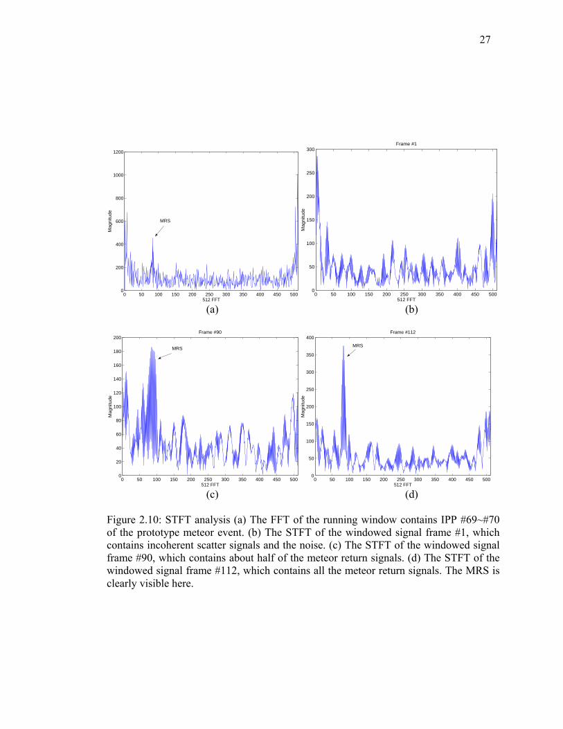
Fig. 2.10 shows the examples of the STFT for different windowed signal frames.
We use #69~#70 IPPs (window size 2) of the prototype meteor event shown in Fig. 2.1
for the demonstration. Fig. 2.10(a) shows the frequency spectrum of the running
window using the whole IPP signals. We can see a weak MRS in the plot. Fig. 2.10(b)
shows the STFT of the windowed signal frame #1, which contains incoherent scatter
signals and the noise. Fig. 2.10(c) shows the STFT of the windowed signal frame #90,
which contains about half of the meteor return signals (23 signal samples). We can see
the MRS rises up from the noise level. Fig. 2.10(d) shows the STFT of the windowed
signal frame #112, which contains all the meteor return signals. The MRS is clearly
visible here. We can see the noise level is much lower in Fig. 2.10(d) compare to Fig.
2.10(a), which makes the meteor easily be detected.
27
0 50 100 150 200 250 300 350 400 450 5000
200
400
600
800
1000
1200
512 FFT
Mag
nitu
de
MRS
0 50 100 150 200 250 300 350 400 450 5000
50
100
150
200
250
300Frame #1
512 FFTM
agni
tude
(a) (b)
0 50 100 150 200 250 300 350 400 450 5000
20
40
60
80
100
120
140
160
180
200Frame #90
512 FFT
Mag
nitu
de
MRS
0 50 100 150 200 250 300 350 400 450 5000
50
100
150
200
250
300
350
400Frame #112
512 FFT
Mag
nitu
de
MRS
(c) (d) Figure 2.10: STFT analysis (a) The FFT of the running window contains IPP #69~#70 of the prototype meteor event. (b) The STFT of the windowed signal frame #1, which contains incoherent scatter signals and the noise. (c) The STFT of the windowed signal frame #90, which contains about half of the meteor return signals. (d) The STFT of the windowed signal frame #112, which contains all the meteor return signals. The MRS is clearly visible here.

28
Del
ayTr
ansv
ersa
lFi
lter
LMS
∑
[]
rn
+−[]
yn
[]
xn
Figu
re 2
.11:
Blo
ck d
iagr
am o
f the
LM
S ad
aptiv
e fil
ter.

29
1z−
1z−
z−∆
0w1w
1Mw−
2Mw−
∑∑
∑
∑×
µ
[]
xn
+−[]
yn
[]
rn
Figu
re 2
.12:
Sys
tem
stru
ctur
e of
the
LMS
adap
tive
filte
r.

30
2.5 Adaptive Filter Technique for the Meteor Observation Data
To separate the incoherent scatter signals from other signals (meteor, white
noise) we apply a Least-Mean-Square (LMS) adaptive filter [19] to the received radar
signals. Fig. 2.11 and Fig. 2.12 are the block diagram and the system structure of the
adaptive filter. The signals, r[n], x[n], and y[n] in the diagram are the received,
estimated, and desired signals, respectively. The z−∆ , #w , and µ in the diagram are the
delay (measured in units of the sampling period), filter coefficients, and the step size,
respectively. The LMS adaptation algorithm is describes as the following [19]:
[ ] [ ] [ ]ˆˆ Hx n n n= −∆w r (2.27)
[ ] [ ] [ ]y n r n x n= − (2.28)
[ ] [ ] [ ] [ ]ˆˆ ˆ1n n n y nµ ∗+ = + −∆w w r (2.29)
where [ ] [ ] [ ] [ ]ˆ , 1 ,..., 1T
n r n r n r n M − ∆ = −∆ −∆ − −∆ − + r is the input vector, µ is
the step size, [ ] [ ]0 1 1ˆ , ,..., TMn w w w −=w is the weight (filter coefficient) vector, the
superscript H denotes Hermitian transposition (transposition combined with complex
conjugation), and the superscript ∗ denotes the complex conjugation. The weights are
recursively adjusted by the LMS algorithm to minimize the mean-square error between
input and output signals. The step size µ determines how fast the filter converges to the
minimum error. (Please refer to [19] for the details of the LMS adaptive filter.) This
system is also called adaptive line enhancer (ALE) [19] which is used to detect a
sinusoidal signal buried in a noise background. The input and output of the transversal
filter are the delayed version of input signal and the estimated input signal, respectively.

31
When the input signals only consist of the white noise and incoherent scatter signals,
which is usually the case since the meteor signal is rare, the transversal filter is a low
pass filter (the frequency response is adaptively adjusted according to the input signal)
which separates the incoherent scatter signal (x[n]) and the white noise(y[n]). In
practice we first use the data with incoherent scatter and white noise signals to train this
system. After it converges, we apply the meteor observation data as the input to the
system and adjust the step size so that the filter responses slowly when there are meteor
return signals. The meteor signals will then appear in y[n] (without incoherent scatter
signals) as the result.
2.6 Experimental Results
In this section, we apply the algorithms described in section 2.2 ~ 2.5 to detect
the meteor return signals of the radar data from Arecibo Observatory. We choose two
relatively low SNR meteor return events shown in Fig. 2.13 and the one shown in Fig.
2.1 as the examples.

32
IPP Number
Alti
tude
(km
)
20 40 60 80 100 120 140 16085
90
95
100
105
110
115
120
(a)
IPP Number
Alti
tude
(km
)
20 40 60 80 100 120 140 16085
90
95
100
105
110
115
120
(b)
Figure 2.13: Real part of complex voltages of two different meteor events. (a) This event was recorded at 07:40:13.000 AST 24 Feb 2001. (b) This event was recorded at 07:40:18.192 AST 24 Feb 2001.

33
2.6.1 MRS Detection
We first apply the sliding window FFT to detect the MRS of the received signals.
We choose the window size 2 which yields the minimum missed detection probability
as shown in Fig. 2.8. Fig. 2.13 shows several examples of the frequency spectrum of
sliding window and the results of the MRS correlator. The highest estimated SNR for
the examples shown in Fig. 2.13(b) is approximately 30 dB, and the lowest SNR shown
in Fig. 2.13(f) is approximately -10 dB. The low frequency part of the spectrum is due
to elemental incoherent scatter [5]. The incoherent scatter can be separated from the
meteor return signal because of its near orthogonality1 with the meteor return signal in
the frequency domain. It is obvious that the MRS correlator raises the peak higher
above the noise level compared to the original frequency spectrum, which increases the
probability of detection. Notice that for the event of IPP #127~128 in Fig. 2.13(b), it is
very difficult to visually identify the meteor return signal.
2.6.2 Filterbank Detection
Fig. 2.15 shows the results of the filter bank for different meteor return signals.
For high SNR meteor return signal, shown in Fig. 2.15(a), the output of the filter bank,
shown in Fig. 2.15(b), is approximately a perfect triangle pattern. For low SNR cases,
shown in Fig. 2.15 (c) and (e), the triangle patterns are noisy. Notice that the position of
the peak of this triangle pattern corresponds to the estimated Doppler velocity and the
altitude of the meteor. For example, the estimated Doppler velocity and the altitude of
1 The frequency spectrums of the meteor and elemental incoherent scatter are both sinc functions. The side lobes of two different signals interact with each other but the effect is mild. We use “near orthogonality” to address this effect.

34
Fig. 2.15(b) are 55.3 km/sec and 100.6 km, respectively. We use this result to
reconstruct the signal that matches the original one, as shown in Fig. 2.15(a), perfectly.
We then use a computer program which combines MRS and filter bank methods
to automatically detect meteor events and determine the Doppler frequency and altitude
of each event. We use the data recorded on February 24 2001. Fig. 2.16 shows the
experimental result. We detect approximately 2000 events. The comparison of this
result with the visually detecting result2 shows that our algorithm can detect more
meteor events.
2.6.3 Short Time Fourier Analysis
Fig. 2.17 shows some results of the running window FFT using the whole IPP
and the results using STFT analysis for comparison. The left hand side plots are the
results of the running window FFT using the whole IPP; the right hand side plots are the
STFT analysis results which yield the maximum peak. Fig. 2.17(b) is the STFT of the
signal sample number 183~227 from two IPPs of the meteor event shown in Fig.
2.13(a), which is the best estimation of the meteor event location. Fig. 2.17(d) is the
STFT of the signal sample number 129~173 of the meteor event shown in Fig. 2.13(b),
which is also the estimated meteor event location. We can see that the noise level is
lower and the MRS shows up more clearly in the STFT analysis results, which makes
the meteor detection easier. The drawback of this technique is we need much more
computing power compared to the running window FFT using the whole IPP.
2 The authors of previous works [4, 7] visually detect and analyze the raw data. For the very weak meteor events, as shown in Fig. 2.10(b) IPP #127~#128, it would be easily missed.

35
0 100 200 300 400 5000
500
1000
1500
512 FFT
Mag
nitu
de
0 100 200 300 400 5000
2
4x 10⁵
Mag
nitu
de
Meteor
Incoherent Scatter
0 100 200 300 400 5000
1
2x 10⁴
512 FFT
Mag
nitu
de
0 100 200 300 400 5000
5
10x 106
Mag
nitu
de
(a) (b)
0 100 200 300 400 5000
1000
2000
512 FFT
Mag
nitu
de
0 100 200 300 400 5000
2
4x 10⁵
Mag
nitu
de
0 100 200 300 400 5000
500
1000
1500
512 FFT
Mag
nitu
de
0 100 200 300 400 5000
2
4x 10⁵
Mag
nitu
de
(c) (d)
0 100 200 300 400 5000
5
10x 105
Mag
nitu
de
0 100 200 300 400 5000
500
1000
1500
512 FFT
Mag
nitu
de
0 100 200 300 400 5000
2
4x 10⁵
Mag
nitu
de
0 100 200 300 400 5000
1000
2000
512 FFT
Mag
nitu
de
Very Weak Meteor
Very Weak Meteor
(e) (f) Figure 2.14: Examples of the MRS detector. These plots are the magnitude of frequency spectrum of different window from the three different meteor event examples (upper plot) and the results of the MRS correlator (lower plot). (a) IPP #70~71 of the meteor event shown in Fig. 2.1. (b) IPP #85~86 of the meteor event shown in Fig. 2.1. (c) IPP #85~86 of the meteor event shown in Fig. 2.13(a). (d) IPP #87~88 of the meteor event shown in Fig. 2.13(a). (e) IPP #68~69 of the meteor event shown in Fig. 2.13(b). (f) IPP#127~128 of the meteor event shown in Fig. 2.13(b).

36
85 90 95 100 105 110 115 120−200
−150
−100
−50
0
50
100
150
200
Altitude (km)
Vol
tage
Doppler Velocity (km/sec)
Altitude
(km)
Relativ
e Pow
er Int
ensity
Meteor
(a) (b)
85 90 95 100 105 110 115 120−15
−10
−5
0
5
10
15
Altitude (km)
Vol
tage
Doppler Velocity (km/sec)
Alti
tude
(km
)
Rel
ativ
e Pow
er Int
ens ity
Meteor
(c) (d)
85 90 95 100 105 110 115 120−15
−10
−5
0
5
10
15
Altitude (km)
Vol
tage
Altitude
(km)
Doppler Velocity (km/sec)
Rel
ativ
e Pos
er Int
ensity
Meteor
(e) (f) Figure 2.15: Examples of the meteor detection using the filter bank. These plots are the real part of the complex voltage and the results of the filter bank. (a) and (b) are IPP #85 of the event shown in Fig. 2.1. (c) and (d) are IPP #87 of the event shown in Fig. 2.13(a). (e) and (f) are IPP #128 of the event shown in Fig. 2.13(b).

37
20 40 60 80 100 120 140 160 180 20085
90
95
100
105
110
115
120
125
Doppler Frequency (kHz)
Alti
tude
(km
)
(a)
85
90
95
100
105
110
115
120
125
0 20 40 60 80 100 120 140 160 180
Alti
tude
(km
)
Event Number (b)
Figure 2.16: Results of automated detection process (a) The scatter plot of Doppler frequency vs.altitude for the meteor events. (b) The histogram of the distribution of the altitude. The histogram of the Doppler frequency is shown in Fig. 2.6 (b).

38
0 50 100 150 200 250 300 350 400 450 5000
200
400
600
800
1000
1200
1400
1600
1800
512 FFT
Mag
nitu
de
MRS
0 50 100 150 200 250 300 350 400 450 5000
100
200
300
400
500
600
700
512 FFT
Mag
nitu
de
MRS
(a) (b)
0 50 100 150 200 250 300 350 400 450 5000
200
400
600
800
1000
1200
1400
1600
1800
512 FFT
Mag
nitu
de
MRS
0 50 100 150 200 250 300 350 400 450 5000
50
100
150
200
250
300
512 FFT
Mag
nitu
de
MRS
(c) (d) Figure 2.17: Comparison of the running window FFT using the whole IPP and the STFT analysis. The window size is 2. The left hand side plots are the results of the running window FFT using the whole IPP. The right hand side plots are the STFT analysis results which yield the maximum peak. (a) and (b) are IPP #85~#86 from the meteor event shown in Fig. 2.13(a). (c) and (d) are IPP #127~#128 from the meteor event shown in Fig. 2.13(b).

39
2.6.4 Adaptive Filter
We experimentally choose the length of the weight vector to be 8 and the time
delay ∆ to be 1. In other words we use [ ] [ ]1 ,..., 8r n r n− − to estimate [ ]r n . Fig. 2.18
shows the results of applying the adaptive filter to the prototype meteor event shown in
Fig. 2.1 and the corresponding frequency spectrums. Fig. 2.18 (a) and (b) are the real
part of the complex voltages of IPP #150 and its frequency spectrum, respectively. Fig.
2.18 (c) and (e) are the [ ]x n and [ ]y n shown in Fig. 2.12. Fig. 2.18 (d) and (f) are the
frequency spectrums of Fig. 2.18 (c) and (e), respectively. We can see that the adaptive
filter almost perfectly estimates the incoherent scatter. It essentially is a low pass filter
in this case. Fig. 2.19 shows the frequency response of the adaptive filter. Note that the
frequency response adaptively changes depending on the input signal, but it is always a
low pass filter.
Fig. 2.20 shows the results of applying the adaptive filter to the meteor event
shown in Fig. 2.13(b). Fig. 2.20 (a) and (b) are the real part of the complex voltages of
IPP #71 and its frequency spectrum. We can clearly see the incoherent scatter signal
(low Doppler frequency) both in time and frequency domain. Fig. 2.20 (c) and (d) are
the output of the adaptive filter ( [ ]y n in Fig. 2.12) and its frequency spectrum. We can
see that the incoherent scatter signal is removed by the filter.
Fig. 2.21 shows the results of applying the adaptive filter to the meteor event
shown in Fig. 2.13(a). Fig. 2.21 (a) and (b) are the real part of the complex voltages of
IPP #87 and its frequency spectrum. Fig. 2.21 (c) and (d) are the output of the adaptive
filter and its frequency spectrum. Again, we can see that the incoherent scatter signal is

40
removed by the filter. Note that the adaptive filter also slightly removes some energy of
higher Doppler frequency signals, which causes slightly distortion of the meteor return
signal.
2.6.5 Combination of Techniques
In this section we try to combine different techniques described in Section
2.2~2.5. We first combine the adaptive filter and the MRS correlator. Fig. 2.22(a) shows
the flow chart of the experiment. We first use the adaptive filter to remove the
incoherent scatter signal and then use the MRS correlator to detect the presence of a
meteor event. For the MRS correlator we use window size 2 to do the analysis. Fig. 2.23
shows the results of running window FFT after applying the adaptive filter and the
output of the MRS correlator. Fig. 2.23 (a) and (b) show the frequency spectrum
(incoherent scatter signal removed) of the running window containing IPP #87~#88 of
the meteor event shown in Fig. 2.13(a) and the result of the MRS correlator. Fig. 2.23 (c)
and (d) show the frequency spectrum (incoherent scatter signal removed) of the running
window containing IPP #127~#128 of the meteor event shown in Fig. 2.13(b) and the
result of the MRS correlator. We can see that the incoherent scatter signals are removed
and the correlator raises the MRS higher above the noise level.
Now we combine the adaptive filter, STFT analysis and the MRS correlator. We
use the adaptive filter to remove the incoherent scatter signal first. Then we do the
STFT analysis and use the MRS correlator to detect the meteor. Fig. 2.24 shows some
experimental results. Fig. 2.24 (a) shows the STFT analysis result of the signal samples
#183~#227 from IPP #87 and #88 of the meteor event shown in Fig. 2.13 (a) after

41
applying the adaptive filter. Compared to Fig. 2.17(b), which is the STFT analysis result
without applying the adaptive filter, we can see the incoherent scatter signal is removed.
Fig. 2.24 (b) shows the MRS correlator result of Fig. 2.24 (a). Fig. 2.24 (c) shows the
STFT analysis result of the signal samples #129~#173 from IPP #127 and #128 of the
meteor event shown in Fig. 2.13 (b) after applying the adaptive filter. Again we can see
the incoherent scatter signal is removed. Fig. 2.24 (d) shows the MRS correlator result
of Fig. 2.24 (c). Comparing Fig. 2.23 and Fig. 2.24 we can see the STFT analysis
reduces the noise level and the correlator raises the MRS higher above the noise level,
which make the detection of the meteor event easier.

42
0 50 100 150 200 250−15
−10
−5
0
5
10
15
20
Sample Number
Mag
nitu
de
0 50 100 150 200 2500
100
200
300
400
500
600
700
800
900
1000
256 FFT
Mag
nitu
de
Incoherent Scatter
(a) (b)
0 50 100 150 200 250−10
−8
−6
−4
−2
0
2
4
6
8
10
Sample Number
Mag
nitu
de
0 50 100 150 200 2500
100
200
300
400
500
600
700
800
900
256 FFT
Mag
nitu
de
(c) (d)
0 50 100 150 200 250−15
−10
−5
0
5
10
Sample Number
Mag
nitu
de
0 50 100 150 200 2500
20
40
60
80
100
120
140
160
180
200
256 FFT
Mag
nitu
de
(e) (f) Figure 2.18: Results of the adaptive filter (a) Real part of the complex voltages of IPP #150 of the prototype meteor event. (b) Frequency spectrum of part (a). (c) The estimation of the adaptive filter, x[n] in Fig. 2.12. (d) Frequency spectrum of part (c). (d) The difference between the estimation and the real signal, y[n] is Fig. 2.12. (e) Frequency spectrum of part (d)

43
0 50 100 150 200 2500.1
0.2
0.3
0.4
0.5
0.6
0.7
0.8
0.9
256 FFT
Mag
nitu
de
Figure2.19: Frequency response of the adaptive filter.

44
0 50 100 150 200 250−20
−15
−10
−5
0
5
10
15
20
25
Sample Number
Am
plitu
de
Meteor
0 50 100 150 200 2500
100
200
300
400
500
600
700
256 FFT
Mag
nitu
de
Meteor
(a) (b)
0 50 100 150 200 250−20
−15
−10
−5
0
5
10
15
20
25
Sample Number
Am
plitu
de
Meteor
0 50 100 150 200 2500
100
200
300
400
500
600
256 FFT
Mag
nitu
de
Meteor
(c) (d) Figure 2.20: Results of applying the adaptive filter to the meteor event shown in Fig. 2.13(b). (a) and (b) are the real party of complex voltages of IPP #71 and its frequency spectrum. (c) and (d) are the output of the adaptive filter and its frequency spectrum.

45
0 50 100 150 200 250−15
−10
−5
0
5
10
15
Sample Number
Am
plitu
de
Meteor
0 50 100 150 200 2500
100
200
300
400
500
600
256 FFT
Mag
nitu
de
Meteor
(a) (b)
0 50 100 150 200 250−15
−10
−5
0
5
10
15
Sample Number
Am
plitu
de
Meteor
0 50 100 150 200 2500
50
100
150
200
250
300
350
256 FFT
Mag
nitu
de
Meteor
(c) (d) Figure 2.21: Results of applying the adaptive filter to the meteor event shown in Fig. 2.13(a). (a) and (b) are the real party of complex voltages of IPP #87 and its frequency spectrum. (c) and (d) are the output of the adaptive filter and its frequency spectrum.

46
Ada
ptiv
eFi
lter
MR
SC
orre
lato
r[]
IPP
rn
OU
TPU
T
(a
)
Adap
tive
Filte
rM
RS
Cor
rela
tor
OU
TPU
TS
TFT
Ana
lysi
s[]
IPP
rn
(b
) Fi
gure
2.2
2: F
low
cha
rts o
f the
exp
erim
ents
. (a)
The
com
bina
tion
of th
e ad
aptiv
e fil
ter a
nd th
e M
RS
corr
elat
or. (
b) T
he c
ombi
natio
n of
the
adap
tive
filte
r, th
e ST
FT a
naly
sis a
nd th
e M
RS
corr
elat
or.

47
0 50 100 150 200 250 300 350 400 450 5000
100
200
300
400
500
600
512 FFT
Mag
nitu
de
MRS
0 50 100 150 200 250 300 350 400 450 5000
500
1000
1500
2000
2500
Mag
nitu
de
(a) (b)
0 50 100 150 200 250 300 350 400 450 5000
50
100
150
200
250
300
350
400
450
512 FFT
Mag
nitu
de
MRS
0 50 100 150 200 250 300 350 400 450 500200
400
600
800
1000
1200
1400
Mag
nitu
de
(c) (d) Figure 2.23: Experimental results of combining the adaptive filter and the MRS correlator. (a) and (b) are the frequency spectrum of the running window FFT containing IPP #87~#88 from the meteor event shown in Fig. 2.13(a) and the result of the MRS correlator. (c) and (d) are the frequency spectrum of the running window FFT containing IPP #127~#128 from the meteor event shown in Fig. 2.13(b) and the result of the MRS correlator.

48
0 50 100 150 200 250 300 350 400 450 5000
100
200
300
400
500
600
512 FFT
Mag
nitu
de
MRS
0 50 100 150 200 250 300 350 400 450 5000
500
1000
1500
2000
2500
3000
Mag
nitu
de
(a) (b)
0 50 100 150 200 250 300 350 400 450 5000
50
100
150
200
250
512 FFT
Mag
nitu
de
MRS
0 50 100 150 200 250 300 350 400 450 5000
200
400
600
800
1000
1200
1400
Mag
nitu
de
(c) (d) Figure 2.24: Experimental results of combining the adaptive filter, the STFT analysis and the MRS correlator. (a) The STFT analysis result of signal samples #183~#227 of IPP #87 and #88 from the meteor event shown in Fig. 2.13(a). (b) The result of the MRS correlator. The input is shown in part (a). (c) The STFT analysis result of signal samples #129~#173 of IPP #127 and #128 from the meteor event shown in Fig. 2.13(b). (d) The result of the MRS correlator. The input is shown in part (c).

49
Chapter 3
Interference Detection and Removal
The interference observed in AO meteor observation data could be separated
into two categories: sparse or dense interference. Both of them are non-periodic and
bursty (strong energy). Knowing these properties, we use signal processing techniques
to detect and remove the interference samples in the meteor data. We introduce two
interference detection methods. First, we calculate the central moments of the power
profile of the meteor data (per IPP). When the fraction of the interference signal
samples is very low (sparse interference), the kurtosis (4th central moment) is very high.
We detect the interference by calculating this parameter. Second, we apply a nonlinear
filter to the power profile of the meteor data then calculate the power reduction
percentage to detect the interference. After detecting the interference, we remove the
corresponding interference signal samples.
We model the received signals in Section 3.1. Two detection methods are
described in Section 3.2 and 3.3. The interference removal process is introduced in
Section 3.4. Experimental results are given in Section 3.5.
3.1 Models for the Received Signals
The interference detection is performed IPP by IPP. Assume the received
complex signal for each IPP is [ ], 1, 2,..., IPPr n n N= , where NIPP is the number of signal
samples per IPP. We normalize time, n, with respect to the sampling period for

50
notational convenience. The model for [ ]r n consists of three different signals: (1)
additive complex white noise, [ ]wn n ; (2) meteor return signal, [ ]m n ; (3) interference
signal, [ ]i n .
Let the real and imaginary part of [ ]wn n be , [ ]w rn n and , [ ]w in n , respectively.
Both of them are Gaussian distributed random variables with mean 0 and variance 2σ ,
denoted by 2(0, )N σ .
The meteor return signal, [ ]m n , is modeled as
( ){ } [ ][ ] exp - , 1, 2,...,M D M IPPm n A j n n l n Nω φ= + ∆ = (3.1)
which is the same as (2.1). Note that we use MA for the amplitude of meteor signal.
According to our observations, the energy of the interference is very strong and
the duration is very short. We model the interference signal sample as
{ }int[ ] exp [ ]i n A j nθ δ= (3.2)
where intA is the amplitude, θ is the phase, and [ ]nδ is the unit sample function. There
may be several interference samples in one IPP. To simplify the analysis, we assume all
interference samples within one IPP have the same amplitude.
When all three signals are present in one IPP, [ ]r n is expressed as
int
1[ ] [ ] [ ] [ ], 1, 2,...,
N
w i IPPi
r n n n m n i n p n N=
= + + − =∑ (3.3)
where intN is the number of interference samples, and ip is the position of i-th
interference sample, which is assumed uniformly distributed between 1 and NIPP.
The power profile of [ ]r n in (3.3) is expressed as

51
int2 2 2
1[ ] [ ] [ ] [ ] , 1, 2,...,
N
r w i IPPi
P n n n m n i n p n N=
= + + − =∑ (3.4)
Substituting (3.1) and (3.2) into (3.4), we have
[ ]int2 2 2
int1
[ ] [ ] [ ], 1, 2,...,N
r w M M i IPPi
P n n n A n l A n p n Nδ=
= + ∆ − + − =∑ (3.5)
Note that [ ]rP n is always real and non-negative. We will use [ ]rP n to detect the
presence of the interference.
3.2 Interference Detection: Nonlinear Filter Method
To detect the presence of the interference we first apply a minimum filter of
window size 5 to [ ]rP n . Note that the window size of the minimum filter must be larger
than the duration of one interference, otherwise this method does not work. The output
of the minimum filter, ,min[ ]rP n , is expressed as
{ },min[ ] min [ 2], [ 1], [ ], [ 1], [ 2] , 1, 2,...,r r r r r r IPPP n P n P n P n P n P n n N= − − + + = (3.6)
We ignore samples with indices outside the range 1 IPPn N≤ ≤ . We then calculate the
standard deviation of [ ]rP n and the power reduction percentage (PRP), which is defined
by
( ),min
1
1
[ ] [ ]100%
[ ]
IPP
IPP
N
r rn
N
rn
P n P nPRP
P n
=
=
−= ×∑
∑ (3.7)
Using these two parameters (standard deviation and PRP) we can identify the presence
of interferences. We evaluate these two parameters for three different cases.

52
Case I: [ ]r n consists of additive white Gaussian noise only
Without the presence of the meteor and the interference signals,
[ ], 1, 2,...,r IPPP n n N= are independent and identical chi-square distributed random
variables with 2 degrees of freedom [17]. The probability density function (PDF),
( )pf x , and the cumulative density function (CDF), ( )pF x , of [ ]rP n are [10]
2 2
1( ) exp , 02 2P
xf x xσ σ
= − ≥
(3.8)
2 ( ) 1 exp , 02P
xF x xσ
= − − ≥
(3.9)
The expected value and standard deviation of [ ]rP n are
{ } 2( ) 2rE P n σ= (3.10)
{ } 2( ) 2rStd P n σ= (3.11)
To derive the probability density function of ,min[ ]rP n , we define
{ }( ) Prob [ ]P rR x P n x= > . Then
{ } { },min ,min( ) Prob [ ] Prob [ ] , 2, 1,..., 2P r rR x P n x P n k x k= > = − > = − − (3.12)
Use the independent and identically distributed property, (3.12) becomes
{ }( )5 5,min ( ) Prob [ ] ( )P r PR x P n x R x= > = (3.13)
Note that ( ) 1 ( )P pR x F x= − . The derivative of (3.13) is then
4,min ,min( ) ( ) 5 ( ) ( )P P P P
d R x f x f x R xdx
= − = − (3.14)
Substituting (3.8), (3.9) into (3.14), we have

53
,min 2 2
5 5( ) exp , 02 2P
xf x xσ σ
= − ≥
(3.15)
The expected value of ,min[ ]rP n is
{ } 2,min
2[ ]5rE P n σ= (3.16)
Substituting (3.10), (3.16) into (3.7), we have the expected value of PRP.
{ }{ } { }( )
{ }
2 2,min
12
1
2[ ] [ ] 25100% 80%
2[ ]
IPP
IPP
N
r rn
N
rn
E P n E P nE PRP
E P n
σ σ
σ=
=
− −= × = =∑
∑ (3.17)
Case II: [ ]r n consists of white Gaussian noise and meteor return signals
In this case, [ ], , 1,..., 44r M M MP n n l l l= + + , corresponding to the meteor return
signals, are independent and identical noncentral chi-square distributed random
variables with 2 degrees of freedom with noncentrality parameter 2MA ; other samples
are independent and identical chi-square distributed random variables with 2 degrees of
freedom. The PDF of [ ]rP n is modeled as
( ) ( ) ( )P N Mf x p f x q f x= ⋅ + ⋅ (3.18)
where 45 / IPPq N= , 1p q+ = , ( )Nf x is the PDF of chi-square distribution expressed in
(3.8), and ( )Mf x is the PDF of noncentral chi-square distribution, i.e.,
( )2
02 2 2
1( ) exp , 02 2
M MM
A x Af x I x xσ σ σ
+ = − ≥
(3.19)

54
where 0 (.)I is 0th order modified Bessel function. The expected value and standard
deviation of [ ]rP n are
{ } 2 2[ ] 2r ME P n p A qσ= + (3.20)
{ } 4 2 2 4[ ] 4 4r M MStd P n A q A pqσ σ= + + (3.21)
To evaluate the PRP, we consider the very high SNR meteor return signal case first. For
this case, the noise power is negligible when calculating the PRP, and the power of
meteor signals are approximately equal to a constant, that is
2
2
, , 1,..., 44[ ]
2 , , 1,..., 44M M M M
rM M M
A n l l lP n
n l l lσ = + +
≅ ≠ + +
(3.22)
After applying the minimum filter, the resultant ,min[ ]rP n is
2
,min 2
, 2, 3,..., 42( ) 2 , 2, 3,..., 42
5
M M M M
rM M M
A n l l lP n
n l l lσ
= + + +≅
≠ + + +
(3.23)
Note that after applying the minimum filter with window size 5, we lose 4 samples at
the beginning and the end of the meteor return signals. The approximate PRP is
2 2
2
45 41 100% 9%45M M
M
A APRPA−
≅ × ≅ (3.24)
For lower SNR case the PRP will be larger than 9% but less than 80% (no meteor return
signals).
Case III: [ ]r n consists of noise and interference signals
We assume the interference signals in the same IPP have the same power, i.e.,
2int[ ]rP n A= , n∈{interference signal samples}. Other power profile file samples are chi-

55
square distributed reandom variables with 2 degrees of freedom. The PDF of [ ]rP n is
modeled as
( ) ( ) ( )P N If x p f x q f x= ⋅ + ⋅ (3.25)
where int / IPPq N N= , 1p q= − , intN is the number of interference signal samples,
( )Nf x is the same as in (3.18), and 2int( ) [ ]If x x Aδ= − . The expected value and standard
deviation of [ ]rP n are
{ } 2 2int[ ] 2rE P n p A qσ= + (3.26)
{ } ( )24 4 2 2int int[ ] 8 2rStd P n p A q p A qσ σ= + − + (3.27)
Note that 2intA is much larger than 2σ , so the dominant term for standard deviation is
4intA q , which is proportional to q (the fraction of interference samples in one IPP).
Since the window size of the minimum filter is larger than the duration of the
interference, ,min[ ]rP n is approximately equeal to the one derived in the noise only case,
i.e., (3.12)~(3.16). The expected value of PRP is
{ }{ } { }( )
{ }
( ) 2 2,min1
2 2
1
[ ] [ ] 2 2 / 5100% 100%
2[ ]
N
r rIn
NI
rn
E P n E P n p A qE PRP
p A qE P n
σσ
=
=
− − += × = ×
+
∑
∑(3.28)
Note that PRP is also proportional to q. So the smallest PRP occurs when there is only
one interference sample, i.e., 1/ IPPq N= . According to our observations, 2intA is always
larger than 21000σ ; and the typical meteor observation data contains 250 signal
samples per IPP. Using 2 2int 1000A σ= and 1/ 250q = , the expected [ ]rP n and PRP are

56
equal to 263σ and 93%, which are much larger compared to those without the presence
of the interference.
Fig. 3.1 shows the scatter plot of more than 2000 IPPs using the two parameters.
These results include all three cases we mentioned above. They match the mathematical
derivations very well. The interference IPPs can be detected by applying appropriate
thresholds.
10 20 30 40 50 60 70 80 90 10010
1
102
103
104
105
106
Power Reduction Percentage
Sta
ndar
d D
evia
tion
Non-interferenceInterferencevery high SNR meteor return
noise only
Figure 3.1: The representation of 2281 non-interference and 320 interference IPPs using standard deviation and power reduction percentage as two parameters. We can use thresholds to easily distinguish the interference IPPs.

57
3.3 Interference Detection: Kurtosis Method
When the fraction of interference samples in one IPP is very small, we can use a
simple kurtosis method to detect the presence of the interference. Assume the received
signal, [ ]r n , consists of additive white noise and the interference. Using the signal
model of (3.25), we have
{ }( ){ } ( )( )
( )( ) ( )
4 8 8 6 6 2 2int int int
2 44 4 2 2 2 2int int int
[ ] [ ] 384 144 2
48 2 3 2
r rE P n E P n A q p A q p A q
p A q p A q p A q
σ σ σ
σ σ σ
− = + − + + +
+ + − +(3.29)
Using (3.26) and (3.29), we can calculate the kurtosis.
Fig. 3.2 shows the kurtosis vs. the fraction of interference samples in one IPP.
The interference-to-noise ratio is 1000. Note that when the fraction is less than 1% the
kurtosis is very high. Fig. 3.3 shows one example of AO data recorded at 18:30:11.153
AST 17 October 1998 with sparse interference and the kurtosis of each IPP. The
kurtosis is very high when the sparse interference appears in the IPP. Using this
property, we detect the presence of the sparse interference.

58
0 0.1 0.2 0.3 0.4 0.50
100
200
300
400
500
600
700
800
900
1000
Fraction of Interference Samples
Kur
tosi
s
Figure 3.2: Kurtosis vs. the fraction of interference samples in one IPP

59
IPP Number
Sam
ple
Num
ber
20 40 60 80 100 120
50
100
150
200
250
300
350
Interference
(a)
0 20 40 60 80 100 1200
50
100
150
200
250
300
IPP Number
Kur
tosi
s
(b)
Figure 3.3: An example of the kurtosis method (a) One example of the sparse interferences in the meteor observation data recorded at 18:30:11.153 AST 17 Oct. 1998. We can see few interference signal samples in the image. (b) The kurtosis of each IPP shown in part (a).

60
( ) 2⋅
DetectionMethod
[ ]r n
[ ]rP n
Find
NO
YES
OUTPUT
{ }arg max [ ]rM P n=
Setr[M]=0
( ) 2⋅
'[ ]r n
'[ ]rP n
Figure 3.4: Flow chart of the interference removal process.

61
3.4 Interference Removal Process
After detecting the interference signals, we blank one signal sample with
maximal energy in the IPP. We then apply the detection mechanism to the resultant IPP
again to see if there is any residual interference. If yes, we blank one signal sample with
maximal energy. We recursively do this process until it passes the interference detection
test. Fig. 3.4 shows the flow chart of interference removal. The detection method in the
flow chart could be the nonlinear filter method or the kurtosis method or the
combination of the two methods.
3.5 Experimental Results
In this section we demonstrate some experimental results of interference
removal. We first use real meteor observation data from Arecibo Observatory to show
the result of interference removal. We then synthesize the IPP signals containing both
meteor and interference and use them to show the performance of the combination of
interference removal and meteor detection algorithms. Fig. 3.5 shows the experimental
result of the sparse interference removal. The interference data is the same as the data
shown in Fig. 3.3. For this kind of interference, both kurtosis and nonlinear filter
methods can detect its presence. We use kurtosis method here and set the threshold to
be 50. Fig. 3.5 (a) and (b) show the image, which consists of 128 IPPs, of the real part
of the complex voltage of the meteor observation data and the power profile of IPP #81
containing an interference, respectively. Fig. 3.5 (c) and (d) show the results of the
interference removal of part (a) and (b), respectively. Note that the bursty interference is
removed by the algorithm.

62
Fig. 3.6 shows one example of the dense interference recorded at 06:57:13.560
AST 11 August 2002. Fig. 3.6 (a) and (b) are the real part of the complex voltage of the
IPP signals and the power profile of IPP #33, respectively. We can see many spiky
interference signals here. Fig. 3.6 (c) and (d) show the results of interference removal
using the nonlinear filter method of part (a) and (b), respectively. We set the standard
deviation and the power reduction percentage equal to 1000 and 75% as the thresholds.
The interference signal samples are completely removed in this example. Note that the
kurtosis method does not work for dense interference case because the fraction of the
interference samples in one IPP is too high.
Fig. 3.7 (a) shows the real part of complex voltage of one synthetic meteor data.
We insert the prototype meteor event into the dense interference to examine the
performance of the interference removal mechanism. Fig. 3.7 (b) shows the result. We
use the nonlinear filter method to detect the interference and set standard deviation and
power reduction percentage equal to 1000 and 75%, respectively. We can see the
algorithm removes most of the interference signals. Fig. 3.7 (c) shows one example of
the IPP containing both meteor and interference signals; and Fig. 3.7 (d) shows the
result after interference removal. Fig. 3.7 (e) and (f) show the frequency spectrum of the
window containing IPP #51~54 before and after the interference removal. Comparing
Fig. 3.7 (e) and (f), we can see that it is much easier to detect the meteor after the
interference removal process. Note that there is a residual interference in IPP #53 as
shown in Fig. 3.7 (d), which doesn’t affect the meteor detection. Also note that when
the interference and meteor signals coincide, the algorithm will remove those samples,
which will degrade the performance of meteor detection.

63
IPP Number
Sam
ple
Num
ber
20 40 60 80 100 120
50
100
150
200
250
300
350
Interference
0 50 100 150 200 250 300 3500
5
10
15x 10
4
Sample NumberP
ower
(a) (b)
IPP Number
Sam
ple
Num
ber
20 40 60 80 100 120
50
100
150
200
250
300
350
0 50 100 150 200 250 300 3500
200
400
600
800
1000
1200
Sample Number
Pow
er
(c) (d) Figure 3.5: One example of the sparse interference removal. (a) The sparse interference. (b) Power profile of IPP #81. (c) The result of interference removal of part (a). (d) The power profile of IPP #81 after interference removal.

64
IPP Number
Sam
ple
Num
ber
10 20 30 40 50 60 70 80
50
100
150
200
250
300
350
400
0 50 100 150 200 250 300 350 4000
1
2
3
4
5
6
7
8x 10
4
Sample Number
Pow
er
(a) (b)
IPP Number
Sam
ple
Num
ber
10 20 30 40 50 60 70 80
50
100
150
200
250
300
350
400
0 50 100 150 200 250 300 350 4000
200
400
600
800
1000
1200
Sample Number
Pow
er
(c) (d) Figure 3.6: One example of dense interference removal. (a) The real part of complex voltage of the dense interference recorded at 06:57:13.560 AST 11 Aug. 2002. (b) The power profile of IPP #33. (c) The result of interference removal of part (a). (d) The power profile of IPP #33 after interference removal.

65
IPP Number
Sam
ple
Num
ber
10 20 30 40 50 60 70 80
50
100
150
200
250
300
350
400
Meteor
IPP Number
Sam
ple
Num
ber
10 20 30 40 50 60 70 80
50
100
150
200
250
300
350
400
Meteor
(a) (b)
0 50 100 150 200 250 300 350 400−300
−200
−100
0
100
200
300
Sample Number
Vol
tage
Meteor
0 50 100 150 200 250 300 350 400−250
−200
−150
−100
−50
0
50
Sample Number
Vol
tage
Meteor
Residual Interference
(c) (d)
0 500 1000 1500 20000
5000
10000
15000
Mag
nitu
de
Meteor
0 500 1000 1500 20000
1000
2000
3000
4000
5000
6000
7000
8000
Mag
nitu
de
Meteor
(e) (f) Figure 3.7: One example of the combination of the interference removal and the meteor detection (a) Synthetic meteor data with interferences. (b) The result of interference removal of (a). (c) Real part of the complex voltage of IPP #53 in (a). (d) The result of the interference removal of (c). (e) The frequency spectrum of the window containing IPPs #51~#54 in (a). (f) The frequency spectrum of the window containing IPPs #51~#54 in (b).

66
Chapter 4
Ionosphere Observation Data
The Arecibo 430 MHz Incoherent Scatter Radar (ISR) has been used to observe
the ionosphere and meteors over forty years. Currently the ISR ionosphere observations
are made using 13-baud Barker or 88-baud pseudo-random coded pulses. The meteor
signals have traditionally been treated as the interference in ionosphere observation data.
In this chapter we present signal processing techniques that separate these two different
signals into different geophysically interesting data sets. We use a filterbank followed
by the short time Fourier transform (STFT) analysis to remove the meteor signals from
the incoherent scatter results. By doing this the incoherent scatter data will not be
contaminated and we can also analyze meteor characteristics from the separated signal.
We also use similar interference removal techniques described in Chapter 3 to remove
the interference signal. Some experimental results are given in this chapter.
4.1 Separation of Meteor and Incoherent Scatter Signals
The ISR ionosphere observations are made using Barker coded carrier pulses
with the inter-pulse period (IPP) of 10 milliseconds. The received signals are mixed to
base-band (DC center frequency) and then sampled in in-phase and quadrature-phase
channels. To separate the incoherent scatter and the meteor signals, we first use a
filterbank to detect the meteor then use STFT analysis to remove the meteor signals.
Let the received signals of one IPP be

67
[ ], 1, 2,...,codedr n n N= (4.1)
where N is the number of samples and let the code be
[ ]code [1], [2], , [ ]c c c c M= (4.2)
where M is the code length. The decoded result, a voltage, is written as
1
[ ] [ 1] [ ], 1, 2,...,M
decoded codedk
r n r n k c k n N=
= + − =∑ (4.3)
Notice that the decoded result can be found in transform domain as is done in practice.
Because of the Doppler speed of the meteor, the decoding process effectively uses the
wrong code thus spreading the meteor energy over a sample twice interval the code
length, which deteriorates the result. Fig. 4.1(a) shows the power profiles of the
decoded signals recorded at 22:20:22.990, September 3rd, 2001. A 13 baud Barker code
was used. There is one meteor event in this sequence. Fig. 4.1(b) shows the power
profile of the raw undecoded signal of that meteor event; and Fig. 4.1(c) shows the
power profile of the decoding result using (4.3). In Fig. 4.1(c) the meteor energies
spread in range because it is not decoded correctly, i.e., the decoding assumed zero
Doppler offset. To properly decode meteor signals we need to correct the code for the
Doppler offset that results in a complex-valued code. The modified decoding equation
after multiplication by the appropriate phasor is
1
[ ] [ 1] [ ] D
Mj kT
meteor codedk
r n r n k c k e ω−
=
= + −∑ (4.4)
where Dω is the Doppler frequency of the meteor, and T is the sampling period. Fig.
4.1(d) shows the decoding result using the correct Doppler frequency shifted Barker
code. Note that the decoding result for incoherent scatter signals is now erroneous. The

68
figure shows that we can detect the presence of the meteor with proper threshold and
precisely identify the location of the meteor.
After identifying the meteor, we use the STFT to analyze the corresponding
meteor signals. We use the data shown in Fig. 4.1(b) to illustrate the process. For this
data set a 13-baud Barker coded pulse was transmitted. With this prior knowledge and
the meteor location identified by the Doppler frequency shifted Barker decoder, we get
the Barker coded meteor signals. Let the coded noise free meteor signals be [ ]codedr L ,
[ 1]codedr L + ,…, [ 12]codedr L + , where L is the range gate location of the meteor. Each
meteor signal sample is modeled by
( )[ 1 ] [ ], 1, 2,...,13Dj nTcodedr L n Ae c n nω φ+− + = = (4.5)
where A is the amplitude, Dω is the Doppler frequency of the meteor signals, T is the
sampling period, φ is the phase, and
[ ]Barker,13 [1], [2],..., [13] [1,1,1,1,1, 1, 1,1,1, 1,1, 1,1]c c c c= = − − − − (4.6)
is the 13 Barker code. The STFT of the meteor signals is
[ ] [ ]{ }( ) (2 )
(13 )
( ) (2 )
FFT [ ] [1], [ 1] [2],..., [ 12] [13]
[1] [1], [2] [2],..., FFT
[13] [13]
FFT , ,...,
D D
D
D D
coded coded coded
j T j T
j T
j T j T
M k r L c r L c r L c
Ae c c Ae c cAe c c
Ae Ae
ω φ ω φ
ω φ
ω φ ω φ
+ +
+
+ +
= ⋅ + ⋅ + ⋅
⋅ ⋅ ⋅ ⋅ = ⋅ ⋅
= { }(13 )Dj TAe ω φ+
(4.7)
Note that [ ] [ ] 1, 1,2,...,13c n c n n⋅ = = . We use fast Fourier transform (FFT) to calculate
the frequency spectrum of the meteor signals. Note that we can zero pad the signals to
get more spectrum samples. Fig. 4.2(a) shows the original coded received meteor
signals. The signals after multiplying the 13 Barker code are shown in Fig. 4.2(b). We

69
can clearly see a sinusoidal signal in Fig. 4.2(b). The frequency corresponds to the
speed of the meteor. Equation (4.7) is the frequency spectrum of a sinusoidal signal. If
we zero pad the signals, we have a sinc function in frequency domain. Fig. 4.3 shows
the magnitude of the STFT of the meteor event shown in Fig. 4.1(a). We can clearly see
the meteor energy (sinc function) in the frequency spectrum. To remove the meteor
signals we use the spectrum to estimate the frequency spectrum of meteor signals (sinc
function) and then subtract it from the original spectrum. Fig. 4.4(a) shows the power
profile of the undecoded IPP with meteor removal. Fig. 4.4(b) shows the power profile
of the decoded result, the process removes 90% of the meteor signal energy. Fig. 4.4(c)
shows RTI plot of the Fig. 4.1 results with the meteor return removed.
Fig. 4.5 shows the flowchart of the meteor signal detector and removal. This
figure summarizes the process we just discussed. The input is one IPP signal at a time –
when running a meteor observation program we analyze 4 or more IPPs at a time [5].
Since we don’t know the Doppler frequency of the meteor signals a priori, we construct
a filterbank. Each filter of the filterbank is a Barker decoder with different Doppler
frequency shift. The filter that produces the maximum peak gives the best estimation of
the meteor Doppler frequency. We can increase the resolution of Doppler frequency
estimation by adding more filters. A threshold detector follows the filterbank. When at
least one output of the filters exceeds the threshold we declare meteor detection. We
then remove the meteor signals by STFT analysis, e.g. Fig. 4.3.

70
Time (sec)
Alti
tude
(km
)
1 2 3 4 5 6 7 8 9 10
100
150
200
250
300
350
400
450
500
550
600
Meteor
0 100 200 300 400 5000
1
2
3
4
5
6x 10
4
Sample Number
Pow
er
Meteor
(a) (b)
0 100 200 300 400 5000
1
2
3
4
5
6
7
8
9
10x 10
5
Sample Number
Pow
er
Meteor
0 100 200 300 400 5000
0.5
1
1.5
2
2.5
3
3.5
4
4.5
5x 10
6
Sample Number
Pow
erMeteor
(c) (d) Figure 4.1: Examples of decoding a meteor event (a) Range-Time-Intensity (RTI) plot of 1000 IPPs of decoded ISR data recoded beginning at 22:20:22.990, Sep. 3rd, 2001. Unaveraged power profiles (100 per second) are shown. The E- region appears near 100km altitude while the F-region is above about 230 km altitude. A 13-baud Barker code was transmitted. (b) Power profile of the undocoded meteor event shown in part (a). (c) Power profile of the decoding result of part (b) - incorrect decoding of the Doppler-shifted meteor return spread the meteor return over 26 range-gates. (d) Result of correctly decoding the meteor signal.

71
0 2 4 6 8 10 12 14−200
−150
−100
−50
0
50
100
150
200
250
Mag
nitu
de
Real PartImaginary Part
(a)
0 2 4 6 8 10 12 14−250
−200
−150
−100
−50
0
50
100
150
200
250
Mag
nitu
de
Real PartImaginary Part
(b)
Figure 4.2: Meteor return signal multiplied by the Barker code (a) The Barker coded meteor signals from Fig. 4.1(a). Solid line is the real part of the complex voltages; dot line is the imaginary part of the complex voltages. (b) The result of the signals in part (a) multiplying the 13 Barker code. We can see the sinusoidal signal here. The frequency corresponds to the speed of the meteor.

72
0 100 200 300 400 5000
500
1000
1500
2000
2500
Ma
gn
itud
e
Meteor
Figure 4.3: Magnitude of the Short Time Fourier Transform (STFT) of the Figure4. 1 meteor event.

73
0 100 200 300 400 5000
0.5
1
1.5
2
2.5
3x 10
4
Sample Number
Pow
er
0 100 200 300 400 5000
1
2
3
4
5
6
7x 10
5
Sample Number
Pow
er
(a) (b)
Time (sec)
Altitu
de (k
m)
1 2 3 4 5 6 7 8 9 10
100
150
200
250
300
350
400
450
500
550
600
(c)
Figure 4.4: Result of the meteor signal removal (a) Power profile of the meteor-event-IPP after meteor removal (undecoded). The power profile of original IPP is shown in Fig. 4.1(b). (b) Power profile after decoding and with the meteor removed. (c) RTI presentation of the Fig. 4.1(a) results with the meteor return removed.

74
Bar
ker D
ecod
er
Bar
ker D
ecod
er
Bar
ker D
ecod
er
I N P U T
.......Th
resh
old
Det
ecto
rM
eteo
rS
igna
l
STFT
Anal
ysis
& M
eteo
rR
emov
al
O U T P U T
YES
NO
Figu
re 4
.5: F
low
cha
rt of
the
met
eor s
igna
ls d
etec
tor a
nd re
mov
al.

75
4.2 Interference Removal
The interference observed in AO ISR observation data is very similar to the
sparse interference observed in the meteor data. It usually has strong energy and the
duration is usually very short. We use this short duration property to design a nonlinear
filter to detect and remove the interference. We divide the whole IPP signal into non-
overlapping sectors. Each sector has 50 signal samples. We then compare the strongest
energy signal sample and the 3rd strongest energy signal sample. If the ratio exceeds
certain threshold, we blank the signal sample with strongest energy.
Fig. 4.6 shows the example of the interference removal result. Fig. 4.6 (a) is the
original IPP signal recorded at 1:15:27.542 AST, 22 Mar., 2004. Fig. 4.6 (b) is the
decoded result of part (a). We can see the interference energy spreads twice the code
length which contaminates the result. Fig. 4.6 (c) and (d) are the result of the
interference removal and its decoded result, respectively. We can see that the
interference signal is removed and there is no contamination of the decoded result. Fig.
4.7 shows the image of the decoded results for 1200 IPPs. The start time of this image is
1:15:25.002 AST, 22 Mar., 2004. Each IPP is 10ms. The interference contaminations
are clearly visible here. The arrowheads indicate some of the contaminations. Fig. 4.8
shows the results after interference removal. We can see that the interference
contaminations are removed.

76
0 500 1000 15000
100
200
300
400
500
600
700
800
900
1000
Sample Number
Mag
nitu
de
Interference
0 500 1000 15000
500
1000
1500
2000
2500
3000
Sample NumberM
agni
tude Interference
(a) (b)
0 500 1000 15000
50
100
150
200
250
300
350
400
450
Sample Number
Mag
nitu
de
0 500 1000 15000
500
1000
1500
2000
2500
3000
Sample Number
Mag
nitu
de
(c) (d) Figure 4.6: The example of the interference removal. (a) The IPP signal recorded at 1:15:27.542 AST 22 Mar. 2004. (b) The decoded result of part (a). (c) The result of the interference removal. (d) The decoded result of part (c).

77
Tim
e (
secs
) fr
om
ind
ica
ted
sta
rt t
ime
Sample Number
24
68
10
12
20
0
40
0
60
0
80
0
10
00
12
00
14
00
Inte
rfe
ren
ce
Figu
re 4
.7: T
he d
ecod
ed re
sults
of 1
200
IPPs
.

78
Tim
e (
secs
) fr
om
indic
ate
d s
tart
tim
e
Sample Number
24
68
10
12
200
400
600
800
1000
1200
1400
Figu
re 4
.8: T
he d
ecod
ed re
sults
of 1
200
IPPs
afte
r int
erfe
renc
e re
mob
al.

79
Chapter 5
Other Applications
The meteor observation using the Arecibo Observatory (AO) 430-MHz radar is
made by transmitting 45-µs carrier pulses with an interpulse period (IPP) of 1 ms. The
return signals are demodulated in in-phase and quadrature-phase channels and sampled
at a 1MHz rate. This approach permits the direct observation of the head-echo of the
meteor, which is from the scattering by the free electrons surrounding the meteoroid.
These meteor head echoes are always seen by the large aperture, high power UHF AO
radar. In the contrary the classical meteor trail echoes are rarely seen by the AO radar
because the radar scattering cross-section (RCS) of the trail echo is inversely
proportional to the radar frequency [6]. Using the filterbank algorithm [5, 8] we have
found significant power at low Doppler frequency (near DC) at similar altitude of the
meteor head echo for some meteor events. This result suggests that the AO radar can
occasionally detect the meteor trail-echo.
The hyper-speed meteor is defined as the speed of the meteor is above 72
km/sec. We modified the meteor return signature algorithm [5, 8] which is used as
regular automated meteor searching for the analysis of the meteor observation data from
Arecibo Observatory to search for the hyper-speed meteors. We put two consecutive
inter-pulse period (IPP) signals together and get the frequency spectrum by the FFT.
Then we pass the frequency spectrum through a MRS correlator to detect the presence

80
of the meteor. We then use short time Fourier transform (STFT) to analyze the possible
the hyper-speed events.
5.1 Meteor Trail Echo
We use the filterbank technique described in Section 2.3 to analyze the meteor
trail echo. The filterbank consists of 256 filters. The impulse response of each filter is
45-µs sinusoidal wave correlator with different frequency. The range of the frequency is
from 0 km/sec to 175 km/sec. The resolution of this filterbank is approximately 0.68
km/sec. Fig. 5.1 shows some filterbank results. Fig. 5.1 (a) is the real part of complex
voltages of an IPP signal recorded at 11:48:35.997 AST, 22 February, 2001. Fig. 5.1 (b)
shows the low frequency part of the filterbank output of part (a). We can clearly see
some power at low Doppler frequency (velocity) form the filterbank output. Fig. 5.1 (c)
~ (f) are the other two examples from IPPs recorded at 12:42:25.076 AST and
15:02:47.445 AST, 22 February, 2001, respectively. We can see that sometimes the
power at low Doppler frequency is stronger than the power of the meteor.
5.2 Hyper-Speed Meteor
We modify the MRS detection algorithm described in Section 2.2 to detect the
hyper-speed meteor. We use the running window size 2 and ignore the low frequency
part (< 72 km/sec) of the frequency spectrum for the detection. We also use lower
threshold compared to regular meteor detection. In this way we can detect more weak
events but we also have higher false alarm rate.

81
After detecting the MRS, we then scrutinize the IPP signals. We use a sliding
window Short Time Fourier Transform (STFT) technique, described in Section 2.4, to
further analyze the two IPP signals. Fig. 5.2 shows some results using this method. The
left side plots are the real part of complex voltages. The right side plots are the result of
the STFT which yield the maximum peak. We can see sinusoidal signals in the plots,
which may suggest the existence of hyper-speed meteor. Note that we have only about
half transmitted pulse length signal samples of the sinusoidal wave in Fig. 5.2 (c) from
the beginning of the IPP signal, which means we may lose the first half (22 samples) of
the return signal. In Fig. 5.2 (e) we have two different frequencies sinusoidal waves.
Each of them is about half transmitted pulse length. If the signals are from a hyper-
speed meteor, it may suggest the explosion of the meteoroid. The Doppler velocities of
the three events shown in Fig. 5.2 are 107.60 km/sec, 72.18 km/sec, and 80.36 km/sec,
respectively.
Fig. 5.3 shows an event recorded at 3:36:18.968 AST, 23 February, 2001 and the
analysis results. Fig. 5.3 (a) is the real part of the complex voltages of a running
window containing 2 IPPs. Fig. 5.3 (b) is the result of the running window FFT. Fig. 5.3
(c) is the output of the MRS correlator. Fig. 5.3 (d) shows the result of the STFT
analysis. We can see an unusual peak at high Doppler frequency. But unlike the events
shown in Fig. 5.2 we can not see a sinusoidal wave in time domain, shown in Fig. 5.3
(a). This event may suggest the existence of the hyper-speed meteor event.

82
(a) (b)
(c) (d)
(e) (f) Figure 5.1: The real part of the complex voltage of different meteor events and the results of the filterbank. (a) and (b) are form the meteor event recorded at 11:48:35.997 AST 22 February 2001. (c) and (d) are from the meteor event recorded at 12:42:25.076 AST 22 February 2001. (e) and (f) are from the meteor event recorded at 15:02:47.445 AST 22 February 2001.

83
Sample Number
Am
plit
ud
e
Sinusoidal Signal
256 FFT
Mag
nitu
de
FFT of the Sinusoidal Signal
(a) (b)
Sample Number
Am
plit
ud
e
Sinusoidal Signal
Mag
nitu
de
256 FFT
FFT of the Sinusoidal Signal
(c) (d)
Sample Number
Am
plit
ud
e
Sinusoidal Signal
256 FFT
Mag
nitu
de
FFT of the Sinusoidal Signal
(e) (f) Figure 5.2: The real part of complex voltages of possible hyper-speed meteor events and the results of the STFT analysis. (a) and (b) are recorded at 03:07:24.983 AST 23 February 2001. (c) and (d) are recorded at 20:23:32.198 AST February 2001. (e) and (f) are recorded at 21:26:51.347 AST February 2001.

84
(a) (b)
(c) (d)
Figure 5.3: One example of weak possible hyper-speed meteor event (a) The real part of the complex voltages of an event (2 IPPs) recorded at 3:36:18.968 AST, 23 February, 2001. (b) The frequency spectrum of part (a). (c) The output of the MRS correlator. (d) The result of the STFT analysis

85
Chapter 6
Conclusions and Future Work
6.1 Conclusions
In this work we introduce signal processing techniques for interference removal
and meteor detection for AO meteor and ISR observation data. For meteor observation
data, we present the frequency domain, the time domain, the STFT analysis, and the
adaptive filter signal processing techniques to detect the presence of meteor events. We
use several IPPs simultaneously, and take the Fast Fourier Transform for frequency
domain technique. If a meteor event appears in those IPPs, then we can find a meteor
return signature (MRS) in the frequency spectrum. We convolve the frequency
spectrum with the special structure to distinguish MRS from noise, and find the
estimated Doppler frequency.
For time domain technique, we utilize the prior knowledge of the 45-µs meteor
return signal and construct a filterbank containing 256 filters. We pass one IPP through
the filterbank to estimate both the Doppler frequency and the altitude of the meteor.
Experimental results show that both methods detect meteors very well.
To improve the performance of the frequency domain technique, we use the
STFT to further analyze the meteor event. We take 45 signal samples and do the FFT,
which reduces the noise level in frequency domain. This technique allows us to detect

86
weaker meteor events. We also introduce the adaptive filter to remove the incoherent
scatter signal, which improves the accuracy of the meteor detection.
We use kurtosis or nonlinear filter method to detect and remove the interference
in the meteor observation data. The kurtosis method only works for the sparse
interference while nonlinear filter method works for both sparse and dense interference.
When the interference and meteor signals occur in the same IPP, the algorithm removes
the bursty interference, which makes the meteor detection much easier. Experimental
results show the robustness of the algorithm for meteor detection against the
interference.
For the ISR observation data, we use a filterbank followed by the short time
Fourier transform to remove the meteor signals thus rendering the ionosphere results
more accurate. We can also analyze the separated meteor signals to get parameters, such
as Doppler frequency (speed) and altitude, after the removal, thus providing two
geophysically interesting data streams. We use a nonlinear filter similar to the one
introduced for the meteor observation data to remove the interference. We compare the
strongest and the 3rd strongest signal samples. If the ration exceeds a certain threshold,
we declare a detection of the interference. We then blank the interference signal sample.
6.2 Suggestion for the Future Work
We have proposed several signal processing techniques to solve different
problems. For future work, we can apply these techniques to different applications, such
as the search of the meteor trail echo and the hyper-speed meteor event. We can also
investigate algorithms to save processing time for different techniques, such as

87
filterbank and STFT analysis, to achieve real time process. We will also continue to
invent new techniques and/or improve proposed techniques to get better performance.

88
References
[1] Q. Zhou, C.A. Tepley, and M. P. Sulzer, “Meteor observations by the Arecibo 430
MHz incoherent scatter radar I. Detection, statistics, and interpretation,” Journal
of Atmospheric and Terrestrial Physics 57, pp. 412-431, 1995
[2] J. D. Mathews, D. D. Meisel, K. P. Hunter, V. S. Getman, and Q. Zhou, “Very
high resolution studies of micrometeors using the Arecibo 430 MHz radar,”
Icarus 126, pp. 157-169, 1997
[3] Q. Zhou, P. Perillat, J. Y. N. Cho, and J. D. Mathews, “Simultaneous meteor echo
observations by large aperture VHF and UHF radars,” Radio Science 33, pp.
1641-1654, 1998
[4] D. Janches, J. D. Mathews, D. D. Meisel, V. S. Getman, and Q.-H. Zhou, “Doppler
studies of near-antapex UHF radar micrometeors,” Icarus 143, pp. 347-253,
2000
[5] J. D. Mathews, J. F. Doherty, C.-H. Wen, S. J. Briczinski, D. Janches, D. D.
Meisel, “An update of UHF radar meteor observations and associated signal
processing techniques at Arecibo Observatory,” Journal of Atmospheric and
Solar-Terrestrial Physics, Vol. 65, pp. 1139-1149, July 2003.
[6] J. D. Mathews, “Radio science issues surrounding HF/VHF/UHF radar meteor
studies,” Journal of Atmospheric and Solar-Terrestrial Physics, Vol. 66, pp.
285-299, 2004.
[7] D. Janches, D. D. Meisel, J. D. Mathews, “Orbital properties of the Arecio
micrometeoroids at earth intersection,” Icarus 150, pp. 206-218, 2001

89
[8] C.-H. Wen, J. F. Doherty, J. D. Mathews, “Time-frequency radar processing for
meteor detection,” IEEE Trans. Geosci. Remote Sensing, IEEE Trans., Vol. 42,
Issue 3, 501-510, 2004.
[9] C.-H. Wen, J. F. Doherty, J. D. Mathews, D. Janches, “Meteor detection and non-
periodic bursty interference removal for Arecibo data,” Journal of Atmospheric
and Solar-Terrestrial Physics, Vol. 67, pp. 275-281, February 2005
[10] J. F. Rowe, “Downward transport of nighttime Es-layers into the E-region ar
Arecibo”, Journal of Atmospheric and Solar Terrestrial Physics 36, pp. 225-
235, 1974.
[11] K. L. Miller and L. G. Smith, “Horizontal structure of midlatitude sporadic E
layers observed by incoherent scatter radar”, Radio Science 10, 271-276, 1975.
[12] J. D. Mathews and F. S. Bekeny, “Upper atmosphere tides and the vertical motion
of ionospheric sporadic layers at Arecibo,” Journal of Geophysical Research 84,
2743-2750, 1979.
[13] J. D. Mathews, Y. T. Morton, and Q. Zhou, “Observations of ion layer motions
during the AIDA campaign,” J. Atmos. Terr. Phys., 55, 447-457, 1993.
[14] J. D. Mathews, M. P. Sulzer and P. Perillat, “Aspects of layer electrodynamics
inferred from high-resolution ISR observations of the 80-270 km ionosphere,”
Geophysical Research Letters, 24, 1411-1414, 1997.
[15] M. P. Sulzer, “Meteor Science from Regular Incoherent Scatter Radar Ionospheric
Observations at Arecibo,” Atmos. Chem. Phys. Discuss., 4, 805-831, 2004.

90
[16] J. L. Chau, Woodman, R. F, “Observations of Meteor-Head Echoes Using the
Jicamarca 50 MHz Radar in Interferometer Mode,” Atmos. Chem. Phys., 4, 511-
521, 2003.
[17] John G. Proakis, Digital Communications, 4th edition, McGraw-Hill, 2001
[18] Athanasios Papoulis, Probability, Random Variables, and Stochastic Processes,
3rd edition, McGraw-Hill, 1991.
[19] Simon Haykin, Adaptive Filter Theory, 4th edition, Prentice Hall, 2002.

Vita
Chun-Hsien Wen was born in Tainan, Taiwan in July 1974. In June 1996 he
received the B. Eng. Degree in Electrical Engineering from National Tsing Hua
University, Hsinchu, Taiwan. From August 1999 to December 2001, he was a master
student in the Department of Electrical Engineering, the Pennsylvania State University,
University Park, Pennsylvania, USA. In January 2002, after getting his master’s
degree, he became a Ph.D. student and research assistant in the Department of
Electrical Engineering, the Pennsylvania State University, University Park,
Pennsylvania, USA and has worked on his doctoral degree since then.
His research interests include wireless communication, statistical signal
processing, etc.