
THREE ESSAYS ON MONETARY ECONOMICS -...
99
THREE ESSAYS ON MONETARY ECONOMICS by Mei Dong B.A., Nankai University, 2002 M.A., Simon Fraser University, 2003 a thesis submitted in partial fulfillment of the requirements for the degree of Doctor of Philosophy in the Department of Economics c Mei Dong 2009 SIMON FRASER UNIVERSITY Spring 2009 All rights reserved. This work may not be reproduced in whole or in part, by photocopy or other means, without the permission of the author.
Transcript of THREE ESSAYS ON MONETARY ECONOMICS -...
THREE ESSAYS ON MONETARY ECONOMICS
by
Mei Dong
B.A., Nankai University, 2002
M.A., Simon Fraser University, 2003
a thesis submitted in partial fulfillment
of the requirements for the degree of
Doctor of Philosophy
in the Department
of
Economics
c© Mei Dong 2009
SIMON FRASER UNIVERSITY
Spring 2009
All rights reserved. This work may not be
reproduced in whole or in part, by photocopy
or other means, without the permission of the author.
APPROVAL
Name: Mei Dong
Degree: Doctor of Philosophy
Title of Thesis Three Essays on Monetary Economics
Examining Gommittee:
Chair: Gordon MyersProfessor, Department of Economics
David AndolfattoSenior SupervisorProfessor, Department of Economics
Fernando MartinSupervisorAssistant Professor, Department of Economics
Alexander KaraivanovSupervisorAssistant Professor, Department of Economics
Kenneth KasaInternal Examiner
Professor, Department of Economics
Christopher J. WallerExternal Examiner, Professor and Gilbert SchaeferChair of Economics, University of Notre Dame
Date Approved: Tuesday, March 31, 2009
i i

Last revision: Spring 09
Declaration of Partial Copyright Licence The author, whose copyright is declared on the title page of this work, has granted to Simon Fraser University the right to lend this thesis, project or extended essay to users of the Simon Fraser University Library, and to make partial or single copies only for such users or in response to a request from the library of any other university, or other educational institution, on its own behalf or for one of its users.
The author has further granted permission to Simon Fraser University to keep or make a digital copy for use in its circulating collection (currently available to the public at the “Institutional Repository” link of the SFU Library website <www.lib.sfu.ca> at: <http://ir.lib.sfu.ca/handle/1892/112>) and, without changing the content, to translate the thesis/project or extended essays, if technically possible, to any medium or format for the purpose of preservation of the digital work.
The author has further agreed that permission for multiple copying of this work for scholarly purposes may be granted by either the author or the Dean of Graduate Studies.
It is understood that copying or publication of this work for financial gain shall not be allowed without the author’s written permission.
Permission for public performance, or limited permission for private scholarly use, of any multimedia materials forming part of this work, may have been granted by the author. This information may be found on the separately catalogued multimedia material and in the signed Partial Copyright Licence.
While licensing SFU to permit the above uses, the author retains copyright in the thesis, project or extended essays, including the right to change the work for subsequent purposes, including editing and publishing the work in whole or in part, and licensing other parties, as the author may desire.
The original Partial Copyright Licence attesting to these terms, and signed by this author, may be found in the original bound copy of this work, retained in the Simon Fraser University Archive.
Simon Fraser University Library Burnaby, BC, Canada
Abstract
The thesis consists of three essays on monetary economics. In particular, I focus on using
modern monetary theory with explicit microfoundations to address issues in macroeconomics
concerning the effects of inflation and the coexistence of multiple assets.
The first essay is motivated by the observation that economies undergoing high infla-
tion often experience a reduction of variety in the marketplace. Existing models study how
inflation affects quantity, but few have studied how inflation affects variety. In a monetary
model with explicit microfoundations, I analyze how inflation affects variety as well as quan-
tity. I consider two pricing mechanisms – bargaining and price posting with directed search.
I show that inflation reduces both quantity and variety under both pricing mechanisms.
Quantitatively, the model implies that the total welfare cost of 10% inflation ranges from
4.77% to 8.4% under bargaining and is 1.52% under price posting.
In the second essay, I study an economy in which money and credit coexist as means
of payment and the settlement of credit requires money. The model extends recent devel-
opments in microfounded monetary theory to address the choice of payment methods and
the effects of inflation. Whether a buyer uses money or credit depends on the fixed cost
of credit and the inflation rate. Based on quantitative analysis, the model suggests that
the relationship between inflation and credit exhibits an inverse U-shape which is broadly
consistent with the evidence. Compared to an economy without credit, allowing credit as
a means of payment affects the economy’s money demand, welfare and the welfare cost of
inflation.
In modern monetary theory, money is viewed as a substitute for the record-keeping
technology. In the third essay, my coauthor and I investigate whether one money constitutes
a perfect substitute for the record-keeping technology in a quasi-linear environment, where
private information and limited commitment are present. We adopt the mechanism design
iii

approach and solve a planner’s problem subject to various constraints. The result is that
when money is divisible, concealable and in variable supply, one money may not be sufficient
to replace the record-keeping technology. We further show that two monies are a perfect
substitute for the record-keeping technology.
Keywords : Inflation; Variety; Welfare; Money; Credit; Mechanism Design
iv

To my parents, Baokun and Xinmin, and my husband, Yong: for their love and support.
I love you.
v
Acknowledgments
I am indebted to Dr. David Andolfatto, who teaches me that simple is beautiful, for his
supervision and guidance throughout my academic endeavors at Simon Fraser University.
I appreciate the time and effort that he has spent helping me finish this thesis. I am very
grateful to Dr. Fernando Martin and Dr. Alexander Karaivanov for their support and
encouragement. I have learned so much through numerous discussions with them.
I would like to thank Dr. Ken Kasa and Dr. Christopher Waller for their valuable
comments and suggestions on my thesis. My special thanks go to Dr. Randall Wright, who
introduces me to search theoretic monetary theory and offers me enormous insights on many
aspects.
I should thank all faculty members at the Department of Economics, especially Dr.
Geoffrey Dunbar, Dr. Stephen Easton, Dr. Simon Woodcock and Dr. Jenny Xu for their
generous support throughout this degree. I also appreciate the help from the Department’s
supporting staff, especially Tim Coram, Kathy Godson, Laura Nielson, Kathleen Vieira-
Ribeiro and Gwen Wild.
Last but not least, thank you to all my friends (you know who you are).
vi
Contents
Approval ii
Abstract iii
Dedication v
Acknowledgments vi
Contents vii
List of Tables x
List of Figures xi
1 Inflation and Variety 1
1.1 Introduction . . . . . . . . . . . . . . . . . . . . . . . . . . . . . . . . . . . . . 1
1.2 Environment . . . . . . . . . . . . . . . . . . . . . . . . . . . . . . . . . . . . 4
1.3 Monetary Equilibrium with Bilateral Bargaining . . . . . . . . . . . . . . . . 7
1.3.1 Households . . . . . . . . . . . . . . . . . . . . . . . . . . . . . . . . . 7
1.3.2 Firms . . . . . . . . . . . . . . . . . . . . . . . . . . . . . . . . . . . . 9
1.3.3 Equilibrium . . . . . . . . . . . . . . . . . . . . . . . . . . . . . . . . . 9
1.3.4 Inflation and Variety . . . . . . . . . . . . . . . . . . . . . . . . . . . . 12
1.4 Monetary Equilibrium with Price Posting . . . . . . . . . . . . . . . . . . . . 13
1.4.1 Equilibrium . . . . . . . . . . . . . . . . . . . . . . . . . . . . . . . . . 14
1.4.2 Inflation and Variety . . . . . . . . . . . . . . . . . . . . . . . . . . . . 16
1.5 Quantitative Analysis . . . . . . . . . . . . . . . . . . . . . . . . . . . . . . . 17
1.6 Extension . . . . . . . . . . . . . . . . . . . . . . . . . . . . . . . . . . . . . . 20
vii
1.7 Conclusion . . . . . . . . . . . . . . . . . . . . . . . . . . . . . . . . . . . . . 22
1.8 Appendix . . . . . . . . . . . . . . . . . . . . . . . . . . . . . . . . . . . . . . 23
1.8.1 Proof of Proposition 1.2 . . . . . . . . . . . . . . . . . . . . . . . . . . 23
1.8.2 Proof of Proposition 1.3 . . . . . . . . . . . . . . . . . . . . . . . . . . 24
1.8.3 Proof of Proposition 1.4 . . . . . . . . . . . . . . . . . . . . . . . . . . 24
1.8.4 Proof of Lemma 1.5 . . . . . . . . . . . . . . . . . . . . . . . . . . . . 25
1.8.5 Proof of Lemma 1.6 . . . . . . . . . . . . . . . . . . . . . . . . . . . . 25
1.8.6 Proof of Proposition 1.8 . . . . . . . . . . . . . . . . . . . . . . . . . . 26
1.8.7 Proof of Proposition 1.9 . . . . . . . . . . . . . . . . . . . . . . . . . . 27
1.8.8 Proof of Proposition 1.10 . . . . . . . . . . . . . . . . . . . . . . . . . 28
1.9 References . . . . . . . . . . . . . . . . . . . . . . . . . . . . . . . . . . . . . . 28
2 Money and Costly Credit 31
2.1 Introduction . . . . . . . . . . . . . . . . . . . . . . . . . . . . . . . . . . . . . 31
2.2 Environment . . . . . . . . . . . . . . . . . . . . . . . . . . . . . . . . . . . . 35
2.3 Monetary Equilibrium with Enforcement . . . . . . . . . . . . . . . . . . . . . 38
2.3.1 Buyers . . . . . . . . . . . . . . . . . . . . . . . . . . . . . . . . . . . . 38
2.3.2 Sellers . . . . . . . . . . . . . . . . . . . . . . . . . . . . . . . . . . . . 40
2.3.3 Equilibrium . . . . . . . . . . . . . . . . . . . . . . . . . . . . . . . . . 41
2.3.4 Welfare . . . . . . . . . . . . . . . . . . . . . . . . . . . . . . . . . . . 48
2.4 Quantitative Analysis . . . . . . . . . . . . . . . . . . . . . . . . . . . . . . . 49
2.5 Monetary Equilibrium without Enforcement . . . . . . . . . . . . . . . . . . . 54
2.6 Conclusion . . . . . . . . . . . . . . . . . . . . . . . . . . . . . . . . . . . . . 57
2.7 Appendix . . . . . . . . . . . . . . . . . . . . . . . . . . . . . . . . . . . . . . 58
2.7.1 Use of Credit Card Data . . . . . . . . . . . . . . . . . . . . . . . . . . 58
2.7.2 Proof of Lemma 2.1 . . . . . . . . . . . . . . . . . . . . . . . . . . . . 58
2.7.3 Proof of Lemma 2.2 . . . . . . . . . . . . . . . . . . . . . . . . . . . . 59
2.7.4 Proof of Proposition 2.4 . . . . . . . . . . . . . . . . . . . . . . . . . . 59
2.7.5 Proof of Proposition 2.5 . . . . . . . . . . . . . . . . . . . . . . . . . . 60
2.7.6 Proof of Proposition 2.7 . . . . . . . . . . . . . . . . . . . . . . . . . . 61
2.7.7 Proof of Proposition 2.8 . . . . . . . . . . . . . . . . . . . . . . . . . . 61
2.7.8 Proof of Lemma 2.9 . . . . . . . . . . . . . . . . . . . . . . . . . . . . 62
2.8 References . . . . . . . . . . . . . . . . . . . . . . . . . . . . . . . . . . . . . . 62
viii
3 One or Two Monies? 65
3.1 Introduction . . . . . . . . . . . . . . . . . . . . . . . . . . . . . . . . . . . . . 65
3.2 The Physical Environment . . . . . . . . . . . . . . . . . . . . . . . . . . . . . 68
3.3 Limited Commitment and Private Information . . . . . . . . . . . . . . . . . 71
3.4 Monetary Mechanisms . . . . . . . . . . . . . . . . . . . . . . . . . . . . . . . 74
3.4.1 One-Money Mechanisms . . . . . . . . . . . . . . . . . . . . . . . . . 74
3.4.2 Two-Money Mechanisms . . . . . . . . . . . . . . . . . . . . . . . . . . 77
3.5 Extension to Multi-type-agent Models . . . . . . . . . . . . . . . . . . . . . . 81
3.6 Two Monies as A Perfect Substitute for the Record-Keeping Technology . . . 85
3.7 Conclusion . . . . . . . . . . . . . . . . . . . . . . . . . . . . . . . . . . . . . 85
3.8 References . . . . . . . . . . . . . . . . . . . . . . . . . . . . . . . . . . . . . . 86
ix

List of Tables
1.1 Parameter Values in Bargaining Equilibrium . . . . . . . . . . . . . . . . . . . 19
1.2 Welfare Cost in Bargaining Equilibrium . . . . . . . . . . . . . . . . . . . . . 19
1.3 Parameter Values in Price Posting Equilibrium . . . . . . . . . . . . . . . . . 20
1.4 Welfare Cost in Price Posting Equilibrium Equilibrium . . . . . . . . . . . . . 20
2.1 Parameter Values . . . . . . . . . . . . . . . . . . . . . . . . . . . . . . . . . . 49
2.2 Welfare Cost of 10% inflation . . . . . . . . . . . . . . . . . . . . . . . . . . . 53
2.3 Credit Card - Spending Volume and Debt Outstanding . . . . . . . . . . . . . 59
3.1 Preference Shocks . . . . . . . . . . . . . . . . . . . . . . . . . . . . . . . . . . 82
x
List of Figures
1.1 The Effect of an Increase in Inflation . . . . . . . . . . . . . . . . . . . . . . . 16
2.1 Credit to GDP Ratio and Credit to Money Ratio . . . . . . . . . . . . . . . . 32
2.2 Timeline of Events . . . . . . . . . . . . . . . . . . . . . . . . . . . . . . . . . 38
2.3 The Effect of Inflation - Benchmark . . . . . . . . . . . . . . . . . . . . . . . 50
2.4 Comparative Statics - Varying k . . . . . . . . . . . . . . . . . . . . . . . . . 52
2.5 The Effect of Inflation - Endogenous Credit Limit . . . . . . . . . . . . . . . . 57
3.1 Environment . . . . . . . . . . . . . . . . . . . . . . . . . . . . . . . . . . . . 69
3.2 Early Sorting Ineffective with a Single Money . . . . . . . . . . . . . . . . . . 75
3.3 Early Sorting Effective with Two Monies . . . . . . . . . . . . . . . . . . . . . 78
xi
Chapter 1
Inflation and Variety1
1.1 Introduction
It is a stylized fact that extended periods of high inflation are associated with low levels of
economic activity. A classic example is the German hyperinflation of 1919-1923 where shops
remained empty and suppliers, unable to sell their wares, reduced production; see Guttman
and Meehan (1975). More recent examples include many Latin American economies, where
chronically high rates of inflation are associated with prolonged periods of depressed eco-
nomic activity; see McKenzie and Schargrodsky (2003), and Midrigan (2007). Conventional
economic theory can easily account for the inverse relationship observed between inflation
and the level of economic activity. That is, inflation essentially acts as a distortionary tax
in markets that rely heavily on money to facilitate exchange. The distortion caused by
inflation tends to induce agents to substitute non-market activities for market activities.
However, in quantitative terms, the estimated welfare cost of inflation is generally low. In
Cash-in-Advance models, the estimated welfare cost of inflation is less than 1%; see Lu-
cas (2000). Recently, search theoretic based monetary models generate the welfare cost of
inflation up to 3%; see Lagos and Wright (2005).
1A version of this chapter is sceduled to appear in the May 2010 issue of the International EconomicReview. I am grateful to David Andolfatto and Randall Wright for helpful comments and discussions. I alsothank Dean Corbae, Alexander Karaivanov, Janet Hua Jiang, Fernando Martin, three anonymous referees,and participants at Simon Fraser University, the Bank of Canada, the 2007 workshop on Money, Banking,Payment and Finance at the Federal Reserve Bank of Cleveland, SFU-UBC Ph.D. Student Workshop, the2008 Midwest Macro Meetings, the 2008 Canadian Economic Association Annual Meeting, and the 2008North American Summer Meeting of the Econometric Society for feedback.
1
CHAPTER 1. INFLATION AND VARIETY 2
One dimension that is typically ignored by conventional models is that of product va-
riety. As it turns out, there is ample evidence to suggest that high inflation is associated
with a contraction not only in the quantity of goods produced, but also in the variety of
goods offered for sale. For example, Heymann and Leijonhufvud (1995) report that during
periods of high inflation, fewer transactions were realized, the markets became thinner, and
some markets were thinned out of existence altogether. Shevchenko (2004) discusses how,
during the Russian inflation in the 1990s, a significant reduction was noticed in both the
quantity and the variety of goods offered for sale; see also Guardiano (1993). McKenzie
and Schargrodsky (2003) find that product variety – as measured by the number of Stock
Keeping Units offered in supermarkets – fell by almost 15% during the high inflation period
in Argentina during the early 2000s. For the same country, Midrigan (2007) documents that
the rate of net product creation fell from 19% in June 2001 to −8% in June 2002. Dur-
ing Zimbabwe’s hyperinflation in 2007, many consumer items have disappeared altogether,
forcing supermarkets to fill their shelves with empty packaging behind the few goods on
display.
There are good reasons to believe that product variety enhances welfare. Indeed, in
much of the international trade literature, enhanced product variety is highlighted as a
major source of the welfare improvements that stemmed from freer trade. For example,
Broda and Weinstein (2006) estimate that the gains from the greater variety provided from
imported goods is on the order of 3% of GDP per annum for the U.S. from 1972-2001.2
Since variety is evidently important for welfare, and since inflation appears to be related
to product variety, it seems sensible to explore how current estimates of the welfare cost of
inflation might be affected by explicitly modeling the variety dimension. This is the primary
goal of this paper.
There is some discussion of variety in economics. Lancaster (1990) provides a review of
the existing literature. However, few papers in monetary theory discuss variety. Shevchenko
(2004) analyzes the choice of variety in a model with middlemen, but there is no money
in his model. Burdett and Shevchenko (2007) study money and variety in a model with
indivisible money and indivisible goods. Because of the indivisibility, they cannot discuss
2The theoretical model in Broda and Weinstein (2006) is based on the love-of-variety model. However,their model is different from the basic love-of-variety model in that the gains from variety occur not onlybecause individuals simultaneously consume multiple types of goods, but also because individuals enjoyhigher utilities from certain types of goods than other types.
CHAPTER 1. INFLATION AND VARIETY 3
issues related to inflation. Corbae and Narajabad (2007) combine a monetary search model
with a Hotelling model in order to address the choice of variety using a mechanism design
approach. However, they do not analyze the effect of inflation on variety. In a multiple
matching model, Laing, Li and Wang (2007) show that inflation may increase or decrease
the product variety offered by a seller depending on parameter values. In equilibrium, the
aggregate measure of variety is fixed at 1, independent of the inflation rate.
Other papers studying money and specialization include Kiyotaki and Wright (1993),
Shi (1995), Camera et al. (2003) and Ghossoub and Reed (2005). At the individual level, if
an agent is more specialized, it implies that he can produce less varieties of goods. In this
sense, papers that study specialization can also be viewed as studying the choice of variety
at the individual level. Due to the structure of their models, the measure of variety at the
aggregate level is fixed. In contrast, I construct my model to address variety at the aggregate
level. In addition, specialization is often assumed to reduce the marginal cost of production,
e.g. Camera et al. (2003), whereas in my model less varieties only decreases the average
cost of production, but not the marginal cost. It seems more natural to use my model to
study variety instead of specialization. In terms of the welfare cost of inflation, Ghossoub
and Reed (2005) find that the welfare cost of inflation can be higher when specialization is
more important. In their model, inflation leads to less specialization.
To estimate the welfare cost of inflation with endogenous product variety, I consider a
variant of the monetary framework developed by Lagos and Wright (2005) and Rocheteau
and Wright (2005). In particular, I consider a world where households and firms are matched
randomly in a decentralized market and where standard frictions make money essential.
Prior to matching, firms must invest in a potential set of varieties. Each household experi-
ences an idiosyncratic preference shock that determines which variety the household values.
Conditional on a match taking place, if the household’s taste shock corresponds to the firm’s
ability to supply the desired variety, the household trades money for goods. Firms then take
their accumulated money balances and distribute their profits to households in a future cen-
tralized market, while households reaccumulate money balances. As in the standard model,
inflation will affect the return to accumulating money and hence will affect the quantity
produced. Moreover, inflation will now affect the variety of products offered for sale in the
decentralized market.
Several different pricing mechanisms can be considered in the decentralized market. I
begin with bargaining, which is fairly common in monetary theory. Then I consider price
CHAPTER 1. INFLATION AND VARIETY 4
posting with directed search, which is also called competitive search and has been previously
used in labor economics; see Moen (1997) and Acemoglu and Shimer (2001) for references.
Price posting seems to be a very realistic assumption for the application in this paper. It
also delivers sharp analytical results, especially for comparative statics since the equilibrium
is unique. Additionally, the Friedman rule achieves the constrained efficient allocation in
price posting equilibrium.
Not surprisingly, I find that inflation reduces both equilibrium quantity and variety,
which is consistent with the observations stated above. The main intuition is that inflation
reduces the surplus from each trade, which in turn lowers the marginal benefit of investing in
variety. As variety is costly, inflation reduces variety. Since my concern is also to measure the
additional welfare cost of inflation when product variety is endogenous, the model calibrated
to the U.S. money demand data suggests that these additional costs can be substantial,
although it depends on the pricing mechanism in the decentralized market. In bargaining
equilibrium, the welfare cost of inflation due to the reduction of variety can account for more
than half of the total welfare cost of inflation, depending on households’ bargaining power.
In price posting equilibrium, the welfare cost of inflation due to the reduction of variety is
very small. As a theoretical extension, I allow households to consume the alternate varieties
if they do not find the desired variety.
The rest of the paper is organized as follows. Section 2 describes the environment of
the theoretical model. Section 3 analyzes bargaining equilibrium. Section 4 analyzes price
posting equilibrium. Section 5 studies the model quantitatively and assesses the welfare cost
of inflation. I consider an extension of the model in section 6. Finally, section 7 concludes.
1.2 Environment
The economy is populated by two types of agents: households and firms. There is a [0, 1]
continuum of each type. The set of households and the set of firms are H and F , respectively.
Time is discrete and the horizon is infinite. Households and firms are infinitely lived. During
each period, a centralized market (hereafter CM) and a decentralized market (hereafter DM)
open sequentially. The CM and the DM are distinguished as follows. Households and firms
in the CM are centrally located; whereas in the DM, they must meet one-on-one according
to a random search process.
Households work in the CM, consume a general good in the CM and a special good in
CHAPTER 1. INFLATION AND VARIETY 5
the DM; while firms maximize profits by producing the general good in the CM and the
special goods in the DM. Firms are equally owned by all households. Households discount
across periods at the rate β where 0 < β < 1 and firms discount across periods at the rate1
1+rwhere r is the net real interest rate. All goods are non-storable.
In what follows, I restrict attention to stationary allocations. Let x denote the quantity of
the general good consumed by a household and let y denote the hours worked by a household
in any CM. The momentary utility payoff associated with a household is υ(x) − y, where
υ′′ < 0 < υ′, limx→0 υ′(x) = ∞, and limx→∞ υ′(x) = 0.
In the CM, firms distribute their last period’s realized profits, hire labor and produce
the general good. At the same time, firms also make investment decisions for production
in the following DM. I assume that the production technology in the CM is such that one
unit of labor input produces one unit of the general good. In the DM, firms may potentially
produce a wide variety of goods, but each firm f, f ∈ F can produce a unique set of special
goods Φf . That is, if a special good is in Φf , it is not in Φf ′ , for all f ′ 6= f . Each special
good in the set represents a distinct variety.3 For simplicity, the measure of Φf is N, N ∈ R+
for all f ∈ F .
A firm’s ability to produce goods in a given set of varieties depends on its investment in
the CM. In particular, by investing a measure n ∈ [0, N ] of variety at cost k(n) in terms of
the general good, the firm leaves itself with enough flexibility to produce any special good
j ∈ [0, n]. Assume that k′, k′′ > 0, k(0) = 0, and k′(0) = 0. If the firm turns out to produce
q units of a special good j, j ∈ [0, n] in the DM, the cost of production is c(q).4 As usual,
c′ > 0, c′′ ≥ 0 and c(0) = 0.
In the DM, households will have a desire to consume some special goods. I assume
that prior to their meetings, households have the same distribution of preference over each
firm’s set of special goods. Exactly which variety of good is desired is determined by an
idiosyncratic preference shock, which is realized after households are matched with firms.
Preference shocks are i.i.d. across households and across time. Given that a household meets
3There is no consensus on the terminology of variety. Normally variety is measured by a certain classifi-cation criteria. Broadly speaking, as pointed out in White (1977), a particular variety of good might involvea difference in quality, or can pertain to preferences such as desiring a red shirt but not a blue shirt.
4A previous version of the paper assumes that firms invest in capital in the CM for the production inthe DM. In that version, if a firm invests in b units capital in the CM, the firm’s production capacity isconstrained, i.e., c(q) ≤ b. Assuming that firms have the transformation technology to convert 1 unit capitalin the DM into 1 + r units of the general good in the following CM, firms would invest in enough capital forthe DM production. All the results hold with this slightly more complicated environment.
CHAPTER 1. INFLATION AND VARIETY 6
a firm, let ξ(j) be the probability that the household likes the firm’s good j. Meeting with
a firm who has invested in n varieties, the probability for a household to find the good that
he likes is σ(n), where σ′′ ≤ 0 < σ′. One simple way to model this is to assume that each
household’s preference shock is distributed uniformly over the interval [0, N ] in each Φf for
all f ∈ F . Hence, ξ(j) = 1N
and σ(n) = nN
.5 A household with a desire to consume good j
of q units has utility u(q(j)), with u′′ < 0 < u′, u′(0) = ∞ and u(0) = 0.
The matching technology in the DM is constant return to scale, M : R2+ → [0, 1], where
M denotes the aggregate measure of matches that occur between households and firms. Let
α = M denote the fraction of households/firms who make contact with a firm/household.
At the individual level, α is the probability that any given household makes contact with
a firm, or is the probability that any given firm makes contact with a household. Since all
firms specialize in their own production set and the measure of the firms is 1, the aggregate
measure of the actual product variety is ασ(n) in this model.
I now consider as a benchmark, the allocation that would be chosen by a planner who
weights all households equally. In each period, the planner must assign the general good
consumption x and labor y to the household. The planner also instructs all firms to invest
in variety n ∈ [0, N ] for the production of the special goods. Since the investment in variety
is costly, it will generally be desirable to choose some n < N .
Subsequent to the investment n, households and firms are matched together in a random
manner. I assume that the planner must respect the matching technology in the sense that
he cannot insure households against the risk of not finding a match. Given the ex post
realization of each household’s preference shock, only the fraction ασ(n) of households
consume the special goods and only the fraction ασ(n) of firms produce the special goods.
In the cases where: [1] a household and a firm are matched; and [2] the household desires a
good in the set of varieties [0, n], the household will be assigned consumption q in the DM,
and the firm will produce q units output. In all other cases, the household receives zero and
5Another example of preference distribution models households’ preferences as a symmetrically truncatednormal distribution over the goods [0, N ] in each Φf for f ∈ F ;
ξ(j) =1δλ( j−µ
δ)
Λ(N−µ
δ) − Λ( 0−µ
δ)
where λ(·) is the probability density function of a standard normal distribution and Λ(·) is the cumulativedensity function. The mean corresponds to the good that is most likely to be chosen by households and thevariance represents the dispersion of the ex ante preference. In this situation, σ(n) =
∫ a+n
aξ(j)dj such that
ξ(a) = ξ(a + n). One can show that σ′(n) > 0 and σ′′(n) < 0.
CHAPTER 1. INFLATION AND VARIETY 7
the firm produces nothing.
The planner’s objective can be stated as follows:
maxx,n,q
υ(x) − x − k(n) + ασ(n)[u(q) − c(q)] . (1.1)
At an interior solution (assuming N is sufficiently large), the optimal allocation is charac-
terized by
υ′(x∗) = 1, (1.2)
u′(q∗) = c′(q∗), (1.3)
k′(n∗) = ασ′(n∗)[u(q∗) − c(q∗)]. (1.4)
Note that the planner’s solution has the flavor of a credit arrangement. In particular,
households who find the desired special goods want to make a purchase. By construction,
they have nothing to offer the firm, except the implicit promise of producing a quantity of
the general good the next period (an object that the firm does value).
1.3 Monetary Equilibrium with Bilateral Bargaining
As is standard, I introduce an essential role for money by assuming that agents are
anonymous and lack commitment. Let M denote the aggregate money supply at any given
date. The money supply grows at a gross rate γ. Money is injected (or withdrawn) via a
lump-sum transfer (or tax) only to households at the beginning of each period. The transfer
is τ = (γ − 1)M−, where M− denotes money supply in the previous period.
As all agents are centrally located in the CM, I assume that it is a competitive spot
market (where money is exchanged for the general good). In the CM, households will be
induced to accumulate money balances as money will be the only way in which they can
purchase their desired special goods later. When households and firms meet individually in
the DM, I assume that the exchange of money for good is dictated by a generalized Nash
bargaining solution concept.
1.3.1 Households
Let φ denote the competitive-determined value of money in the CM (i.e., the inverse of
the price level). Let m denote the nominal money balance for a household at the beginning
CHAPTER 1. INFLATION AND VARIETY 8
of the CM. Likewise, let m denote the money balance carried forward into the DM by a
household. Let W and V denote the value functions associated with a household in the
CM and the DM, respectively. Finally, let π denote a firm’s current period expected profit
measured in terms of the general good. Firms’ profits are realized at the beginning of the
next period, so let Π denote the realized aggregate profit measured in terms of the next
period’s general good.6 Since firms are owned by households, each household receives Π− at
the beginning of the CM, where Π− denotes the realized aggregate profit from last period.
At the beginning of each period, a household’s choice problem is
W (m) = maxx,y,m
υ(x) − y + V (m)
s.t. φ(m − m − τ) + x = y + Π−,
or
W (m) = φ(m + τ) + Π− + maxx,m
υ(x) − x − φm + V (m) . (1.5)
The first order conditions are
υ′(x) = 1, (1.6)
V ′(m) = φ. (1.7)
The optimal x is determined in (1.6), which corresponds to the planner’s choice. The optimal
m in (1.7) does not depend on m. From the envelope condition, W ′(m) = φ. Note that
W (m) is linear in m. In particular, W (m) = W (0) + φm.
As the household enters into the DM, the value function is
V (m) = ασ(n)[u(q) + βW+(m − d)] + [1 − ασ(n)]βW+(m), (1.8)
where W+ denotes the value function in the next period. Each household has probability
α of being matched with a firm. Given that a household and a firm meet, the probability
that a household obtains the desired special good is σ(n). In such an event, the household
spends d units of money in exchange for q units of the special good.
6In aggregate, Π = (1 + r)∑
f∈F
πf , where r is the real interest rate.
CHAPTER 1. INFLATION AND VARIETY 9
1.3.2 Firms
Firms in this environment face a sequence of static problems. At the beginning of each
period, a firm may or may not bring money into the CM depending on whether the firm
made a sale in the previous DM. In any case, firms distribute all of their profits to the
households. The objective of a firm is to maximize the current period’s expected profit.
If a firm is matched with a household and is able to provide the household’s desired
variety, it produces q units of output and receives d units of money from the household.
The value of a sale is −c(q) + 11+r
φ+d for the firm. Note that in this economy, the gross
real interest rate 1 + r is implicitly given by 1β. A firm’s choice problem is
π = maxn
−k(n) + ασ(n)[−c(q) +1
1 + rφ+d]
. (1.9)
In general, the terms of trade (q, d) may depend on n, because forward looking households
and firms should internalize the impact of n on the terms of trade. Therefore, I proceed to
solve the generalized Nash problem to get (q, d).
1.3.3 Equilibrium
Let θ ∈ (0, 1] be the household’s bargaining power. The generalized Nash problem is
maxq,d
[u(q) − βφ+d]θ[−c(q) + βφ+d]1−θ (1.10)
s.t. d ≤ m.
If d < m, the solution for q is given by u′(q) = c′(q) or q = q∗. If d = m, the first order
condition with respect to q can be reduced to
βφ+m =(1 − θ)u(q)c′(q) + θu′(q)c(q)
θu′(q) + (1 − θ)c′(q)≡ g(q). (1.11)
Following Lagos and Wright (2005), one can prove that the constraint d ≤ m always
binds in equilibrium. So the terms of trade are given by d = m and βφ+m = g(q). It follows
that dqdm
= βφ+
g′(q) > 0, where g′(q) > 0.
It is interesting to note that the choice of (q, d) does not depend on n. Households and
firms act as if they do not take the choice of n into consideration during bargaining. This
is not surprising since at the time that a household and a firm decide to trade, the firm has
already made the investment in n. The household does not internalize the cost of variety
CHAPTER 1. INFLATION AND VARIETY 10
during the bargaining process. This is the classical holdup problem associated with the
bargaining solution.
Rewrite (1.8) and (1.9) as follows:
V (m) = βW+(0) + ασ(n)u(q) + [1 − ασ(n)]βφ+m, (1.12)
π = maxn
−k(n) + ασ(n)[1
1 + rφ+m − c(q)]
. (1.13)
Since n does not depend on individual m, the envelope condition gives
∂V (m)
∂m= ασ(n)u′(q)
dq
dm+ [1 − ασ(n)]βφ+. (1.14)
Given that (q, d) do not depend on n, the first order condition for an interior n is
ασ′(n)[g(q) − c(q)] = k′(n). (1.15)
To derive the equilibrium, substitute (1.7) into (1.14),
φ = βφ+[1 − ασ(n)] + ασ(n)u′(q)βφ+
g′(q). (1.16)
As new money is injected only to households, each household carries m = M into the DM.
In the steady state, the gross inflation rate is φφ−
= MM−
= γ. Substituting φ+ = g(q)βm
into
(1.16) and using φφ−
= γ, (1.16) is reduced to
u′(q)
g′(q)= 1 +
i
ασ(n), (1.17)
where i is the nominal interest rate defined by the Fisher equation 1 + i = (1 + r)γ.
Definition 1.1 Bargaining equilibrium is a list (q, d, n) such that (q, n) solves (1.15) and
(1.17), and d = m, where m is given by (1.11).
To prove the main results in bargaining equilibrium, I adopt the following assumption.
Assumption 1: (i) limq→0
u′(q)g′(q) = +∞; (ii) u′(q)
g′(q) is strictly decreasing in q.
Proposition 1.2 A bargaining monetary equilibrium exists iif
maxq
−ig(q) + ασ(n)[u(q) − g(q)] > 0,
where n = arg maxn∈[0,N ]
−k(n) + ασ(n)[g(q) − c(q)].
CHAPTER 1. INFLATION AND VARIETY 11
In short, the condition needed in order for a monetary equilibrium to exist rules out
q = n = 0 as a solution. This seems to be obvious, but this is what can be concluded
without imposing any functional forms of u(q), c(q), σ(n) and k(n). If one is willing to
consider some special form of these functions, the condition for the existence of a monetary
equilibrium is more concrete. For example, if u(q) = 1ρqρ, c(q) = q, σ(n) = n and k(n) = 1
2n2
for 0 < ρ < 1 and N = 1, I can show that a monetary equilibrium exists when i is not too
big.7
Quantity q can be viewed as the intensive margin. Variety n affects the frequency of
trade and hence can be viewed as the extensive margin. In the literature, endogenizing entry
decisions or search intensity can also affect the extensive margin. Rocheteau and Wright
(2005) endogenize the entry decisions by sellers. They show that in bargaining equilibrium,
if monetary equilibrium exists, there must be multiple equilibria. In contrast to their result,
I can only prove that a bargaining equilibrium exists under certain conditions.8 Bargaining
equilibrium can be unique, although I have no formal proof for uniqueness. Lagos and
Rocheteau (2005) endogenize search intensity by buyers. There may be multiple equilibria
in their bargaining equilibrium and they argue that there are several ways to ensure a
unique equilibrium. It seems that different types of extensive margins lead to very different
properties of the equilibrium although they all affect the frequency of trade.
In Rocheteau and Wright (2005), entry decisions by sellers have a thick market effect on
buyers and a congestion effect on sellers. More sellers entering the market directly makes
buyers better off and sellers worse off. Similarly in Lagos and Rocheteau (2005), buyers’
search intensity has a thick market effect on sellers and a congestion effect on buyers. If a
buyer increases his search intensity, it benefits sellers and hurt other buyers. In this paper,
more varieties benefits both households (buyers) and firms (sellers). If a firm offers more
varieties, it increases the probability of trading for both parties in this meeting, but it does
not directly affect other firms’ trading probabilities. In this sense, variety does not have the
”direct” congestion effect.
7A sketch of the proof is given here. Define f(q) = u′(q)g′(q)
− 1 − iασ(n)
where n is given by (1.15). A
monetary equilibrium solves f (q) = 0 and q > 0. It is straightforward that monetary equilibrium existswhen i = 0. As i shifts f(q) down, one can see that for any small ε, there is always an i that makes f(q) < 0for all q > ε. As ε approaches 0, limq→0 f(q) = −∞ with these specific functional forms. So when i is bigenough, f(q) < 0 for all q > 0. There is no monetary equilibrium.
8If assuming that k′(0) > 0 and σ′(0) < ∞, then there exists a q0 ∈ (0, q∗] such that n(q0) = 0. In thisparticular case, one can show that if monetary equilibrium exists, there must be multiple equilibria.
CHAPTER 1. INFLATION AND VARIETY 12
1.3.4 Inflation and Variety
Since bargaining equilibrium may not be unique and since as always when there exist
multiple equilibria, the comparative statics results are different for different equilibria, I
assume that either equilibrium is unique, or if multiple equilibria exist, I focus on the
equilibrium with the highest q.
Proposition 1.3∂q∂γ
< 0 and ∂n∂γ
< 0.
Inflation has negative effects on both the intensive margin and the extensive margin.
When inflation goes up, it distorts households’ incentives to hold money, which in turn
has a negative impact on activities that require money. In general, quantity per trade q
decreases. For firms, producing a smaller quantity lowers the marginal benefit of investing
in variety. Since the marginal cost of variety is increasing in n, the choice of n decreases
as q decreases. In this model, there is no double coincidence of wants meeting in the DM.
All transactions of the special goods have to be done with money. In other words, there
are only single coincidence meetings. Once money is less valuable, it is natural that the
market of the special goods shrinks. Previous models that study money and specialization
usually have the property that less specialization (more varieties at the individual level)
leads to a higher probability of double coincidence meetings. Given that inflation lowers
the trade surplus from single coincidence meetings, inflation may lead to less specialization
because double coincidence meetings become more desirable. While this is interesting to
study, it seems appropriate to assume the absence of double coincidence meetings in the
current application.
Proposition 1.4 q < q∗ and n < n∗. The Friedman rule is the optimal monetary policy,
but the efficient allocation cannot be achieved.
In bargaining equilibrium, distortions come from bargaining and inflation. Before bar-
gaining, households invest in money and firms invest in variety. For γ > β, the double sided
investments create a double holdup problem, which cannot be solved by varying bargaining
power. Acemoglu and Shimer (1999) show that bargaining equilibrium is inefficient in a la-
bor search model when a double holdup problem exists. Hosios’ condition does not give rise
to the efficient outcome in the presence of a double holdup problem. At the Friedman rule,
money is not subject to the holdup problem as noted by Aruoba et al. (2007). However,
CHAPTER 1. INFLATION AND VARIETY 13
investment in variety is still subject to the holdup problem unless θ = 0. Since θ = 0 in
general precludes the existence of a monetary equilibrium, I do not consider θ = 0 in this
paper. As a result, the holdup problem still exists and the efficient allocation cannot be
achieved at the Friedman rule.
1.4 Monetary Equilibrium with Price Posting
As an alternative to bargaining, one can consider price posting in the DM, where prices
are posted before meetings, and agents are able to direct their search towards favorable
terms of trade. There are a variety of ways to formalize this. In particular, one can assume
that prices are posted by firms, or households, or market makers.9 I adopt the market maker
version, where market makers design and open a set of submarkets Ω. At the beginning of
each period, each market maker announces the terms of trade (q, d) and the variety n for
his particular submarket ω ∈ Ω. Note that market makers only announce variety n without
specifying the exact subset of special goods. After exiting the CM, households and firms get
to choose which submarket to visit. Those who direct their search to the same (q, d, n) form
an active submarket. Trade is bilateral and there is random matching in each submarket.
Let Hω and Fω be the measure of households and the measure of firms in submarket ω
for ω ∈ Ω. The market tightness of submarket ω is Qω = Hω
Fω. Since Qω affects agents’
matching probabilities, agents anticipate Qω when they choose among the submarkets. In
equilibrium, the actual Qω should be consistent with agents’ rational expectations.
In the CM, a household has the same value function as (1.5) and a firm has the same
profit function as (1.9). For a household in the DM,
V (m) = maxω∈Ω
αh(Q)σ(n)[u(q) + βW+(m − d)] + [1 − αh(Q)σ(n)]βW+(m) . (1.18)
Here αh(Qω) = M(Hω ,Fω)Hω
= M(Qω,1)Qω
is the probability that a household meets a firm in
submarket ω. I omit the subscript ω of (q, d, n,Q) to reduce notations. For a firm,
π = maxω∈Ω
−k(n) + [−αf (Q)σ(n)c(q) +1
1 + rαf (Q)σ(n)φ+d]
, (1.19)
where αf (Qω) = M(Hω ,Fω)Fω
= M(Qω, 1) is the probability that a firm meets a household.
9Here market makers represent a third party that is not involved in actual trading. Competition amongmarket makers makes them earn zero profit.
CHAPTER 1. INFLATION AND VARIETY 14
Using the results from the previous section,
W (m) = φ(m + τ) + Π− + maxm
−φm + βφ+m + αh(Q)σ(n)[u(q) − βφ+d] + βW+(0) .
(1.20)
1.4.1 Equilibrium
Equilibrium requires that there is no possible submarket that makes some firms better
off without making households worse off. Market makers choose (q, d, n,Q) to maximize
π such that households get the equilibrium expected utility U from the submarkets. The
market maker’s problem is
maxq,d,Q,n
π s.t. W (m) = U .
It can be shown that households choose to bring just enough money d to the DM. Ignoring
the constants in (1.19) and (1.20), the market maker’s problem is reformulated as
maxq,d,Q,n
αf (Q)σ(n)[−c(q) + βφ+d] − k(n) (1.21)
s.t. − [i + αh(Q)σ(n)]βφ+d + αh(Q)σ(n)u(q) = U . (1.22)
where U = U − βW+(0) − φ(m + τ) − Π−.
Since market makers take U and hence U as given, I can denote the set of solutions as
Υ(U) = q(U ), d(U), Q(U ), n(U). Lemma 1 establishes the existence of a solution.
Lemma 1.5 Υ(U) is nonempty and upper-hemicontinuous.
Substituting the expression of βφ+d from (1.22) into (1.21), the unconstrained market
maker’s problem is
maxq,Q,n
αf (Q)σ(n)[−c(q) +αh(Q)σ(n)u(q) − U
i + αh(Q)σ(n)] − k(n)
. (1.23)
Define the elasticity η(Q) = MH(H,F ) HM(H,F ) = MQ(Q, 1) Q
M(Q,1) as households’ contri-
bution to firms’ probability of matching. Firms’ contribution to households’ probability of
matching is 1−η(Q) = MF (H,F ) FM(H,F ) = [M(Q, 1)−QMQ(Q, 1)] 1
M(Q,1) . The first order
CHAPTER 1. INFLATION AND VARIETY 15
conditions for an interior solution of the unconstrained market maker’s problem are
q :u′(q)
c′(q)− 1 −
i
αh(Q)σ(n)= 0, (1.24)
Q : u(q) −U
αh(Q)σ(n)−
u′(q)
c′(q)
η(Q)u′(q)c(q) + [1 − η(Q)]c′(q)u(q)
η(Q)u′(q) + [1 − η(Q)]c′(q)= 0, (1.25)
n : αf (Q)σ′(n)c′(q)[u(q) − c(q)]
η(Q)u′(q) + [1 − η(Q)]c′(q)− k′(n) = 0. (1.26)
The next assumption is used to ensure the uniqueness of price posting equilibrium.
Assumption 2: (i) qu′(q)u(q) is weakly decreasing in q; (ii) qc′(q)
c(q) is weakly increasing in q;
(iii) η(Q) is weakly decreasing in Q.
Commonly used utility functions such as CRRA and CARA utilities satisfy (i). Log
concavity of u′(q) is also sufficient to guarantee (i). Cost functions such as c(q) = qa,
a ≥ 1 satisfy (ii). With regard to (iii), η(Q) is decreasing in Q for the most frequently used
matching functions, such as the Cobb-Douglas matching function, the matching function
in Kiyotaki and Wright (1993) and the urn-ball matching function as in Burdett, Shi and
Wright (2001).
Lemma 1.6 Q(U ) is nonempty, upper-hemicontinuous and strictly decreasing in U .
In price posting equilibrium, households and firms choose the submarket that yields the
highest expected payoff. The formal definition of a price posting equilibrium is given below.
Definition 1.7 A price posting equilibrium is a list of (qω, Qω, dω, nω, Fω) and a U ≥ 0
such that given U , (qω, Qω, dω, nω, Fω) maximize the firm’s expected profit subject to the
constraint that households get U , where U satisfies∑
ωFω = 1, and
∑
ωFωQω = 1.
Proposition 1.8 A price posting monetary equilibrium exists if
maxq,n
αf (Q)σ(n)[−c(q) +αh(Q)σ(n)u(q)
i + αh(Q)σ(n)] − k(n)
> 0,
where Q = Q(0). Moreover, it is unique.
Similar to bargaining equilibrium, I need an extra condition to ensure the existence of
a monetary equilibrium, i.e., q > 0 and n > 0. In contrast to bargaining equilibrium, the
monetary equilibrium is unique. If Q(0) ≥ 1, the market tightness Q should be consistent
with the exogenous supply of households and firms and Q = 1 in equilibrium. Once Q is
CHAPTER 1. INFLATION AND VARIETY 16
determined, (1.24) and (1.26) jointly determine (q, n). In equilibrium, U satisfies (1.25) and
then one can get the market value of a household U . If Q(0) < 1, the only equilibrium
requires U = 0 and Q = Q(0). Here households are indifferent whether to participate the
submarket or not. Again, (1.24) and (1.26) jointly determine (q, n). In either case, the
solution of βφ+d is
βφ+d =η(Q)u′(q)c(q) + [1 − η(Q)]c′(q)u(q)
η(Q)u′(q) + [1 − η(Q)]c′(q)≡ h(q), (1.27)
where I use (1.22) and (1.25).
1.4.2 Inflation and Variety
A nice property of the price posting equilibrium is that it is unique. Hence, I can study
the effects of inflation on quantity and variety without additional assumptions.
Proposition 1.9∂q∂γ
< 0 and ∂n∂γ
< 0.
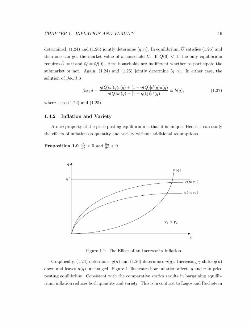
Figure 1.1: The Effect of an Increase in Inflation
Graphically, (1.24) determines q(n) and (1.26) determines n(q). Increasing γ shifts q(n)
down and leaves n(q) unchanged. Figure 1 illustrates how inflation affects q and n in price
posting equilibrium. Consistent with the comparative statics results in bargaining equilib-
rium, inflation reduces both quantity and variety. This is in contrast to Lagos and Rocheteau

CHAPTER 1. INFLATION AND VARIETY 17
(2005), where the price posting equilibrium generates different comparative statics results
from the bargaining equilibrium. In their paper, inflation increases buyers’ search intensity
at low inflation rates because buyers’ surplus from trade increase at low inflation rates. With
endogenous variety, inflation always lowers firms’ surplus from trade. Therefore, investment
in variety also decreases.
Proposition 1.10 n ≤ n∗ and q ≤ q∗. The Friedman rule achieves (q∗, n∗).
In the absence of inflation distortion, the price posting equilibrium achieves the efficient
allocation. This result is in line with the results of Acemoglu and Shimer (1999). The key
factors that make price posting an efficient pricing mechanism include both posting prices
and directed search. Terms of trade (q, d) and variety n are announced before a household
and a firm meet. Households and firms can direct their search towards the submarkets that
are most desirable to them. The timing makes households and firms internalize the impact
of the choices of money holding and variety on the terms of trade, and thereby avoids the
double holdup problem. Suppose that the monetary authority can run the Friedman rule
in order to avoid inflation distortion. Price posting with directed search can solve all other
inefficiencies arising in this environment.
1.5 Quantitative Analysis
The current model predicts that inflation affects both quantity and variety. The main
purpose of this section is to quantify the welfare cost of inflation due to the reduction of
both quantity and variety. Moreover, I decompose the total welfare cost of inflation into the
cost due to quantity and the cost due to variety. It helps to understand how endogenizing
variety contributes to the total welfare cost of inflation.
Suppose that a household’s DM consumption and variety are qτ and nτ at τ% inflation.
In the steady state, let the aggregate welfare at τ% inflation be W(τ). The welfare cost of
τ% inflation is measured by ∆, which is the fraction of consumption that a household would
like to give up to have 0% inflation rather than τ% inflation.10 Formally, ∆ is implicitly
10Here I measure the welfare cost of τ% inflation as the fraction of consumption a household would like togive up for the economy to have 0% inflation rather than τ%. This is a little different from existing welfarestudies using monetary search models, where there is either one type of agent or an endogenous buyer-sellerratio. With only one type of agent, the welfare cost of inflation is simply the fraction of consumption anagent would be willing to give up. With endogenous choice of being a buyer or a seller, e.g. Rocheteau and
CHAPTER 1. INFLATION AND VARIETY 18
given by
W(τ) =1
1 − βυ[x∗(1 − ∆)] − x∗ + ασ(n0)u[q0(1 − ∆)] − c(q0) − k(n0) .
I first fix variety at nτ and determine the fraction of consumption a household is willing
to give up in order to have q0 instead of qτ . This can be viewed as the welfare cost due to
quantity and it is measured by ∆q, where ∆q is from
W(τ) =1
1 − βυ[x∗(1 − ∆q)] − x∗ + ασ(nτ )u[q0(1 − ∆q)] − c(q0) − k(nτ ) .
Next I fix quantity at qτ and determine the fraction of consumption a household is willing to
give up to have n0 instead of nτ . This is the welfare cost due to variety, which is measured
by ∆n from the following equation.
W(τ) =1
1 − βυ[x∗(1 − ∆n)] − x∗ + ασ(n0)u[qτ (1 − ∆n)] − c(qτ ) − k(n0) .
Money demand and nominal interest rate data are from Craig and Rocheteau (2007).
The standard money demand data is computed from L(i) = M/PY , where M is measured
by M1 and PY is the nominal GDP. The nominal interest rate i is annual short term
commercial paper rate. Let υ(x) = a log x, u(q) = q1−ρ
1−ρwhere 0 < ρ < 1, c(q) = Aq,
σ(n) = nn+1 and k(n) = κn2. I use the urn-ball matching function so that α = M = 1−e−1.
I set the real interest rate r = 0.04, which implies that β = 0.9615. The model’s ”money
demand” is:
L(i) = M/PY =1
a(1+i)g(q) + ασ(n)
.
The strategy is to choose (a, ρ,A, κ) to fit the standard money demand observations. Ideally,
parameters related to variety should be calibrated from data related to variety. As it is hard
to obtain these data, I choose all parameters through fitting the money demand. Due to the
identification problem, I fix A = 1, κ = 0.01 and fit (a, ρ) to the data.11 In the following, I
Wright (2004), buyers and sellers get the same expected utility in equilibrium. So the welfare cost of inflationis also measured by the fraction of consumption a buyer or a seller would like to give up. In my model,firms are owned by households. So it is reasonable to study the welfare cost of inflation as the fraction ofconsumption that households would give up.
11I begin by finding values of (a, ρ, κ) together. For price posting equilibrium, the results are quiterobust. For bargaining equilibrium, the results are sensitive to the initial guess of (a, ρ, κ) and the value ofκ is sometimes found to be 0, which makes the equilibrium problematic and hence the welfare calculationimpossible. I choose to fix κ at 0.01, which is in the range of its values in the above exercise. Because fixingκ = 0.01 causes very small loss of fit, and because the welfare results from choosing (a, ρ, κ) if available, arevery similar to what are reported below, I use the results from fixing κ and only choosing (a, ρ).
CHAPTER 1. INFLATION AND VARIETY 19
study the welfare cost of 10% inflation. As a benchmark, I consider a quantitative version
of the model where there is no endogenous variety choice. That is, σ(n) = 1 and k(n) = 0.
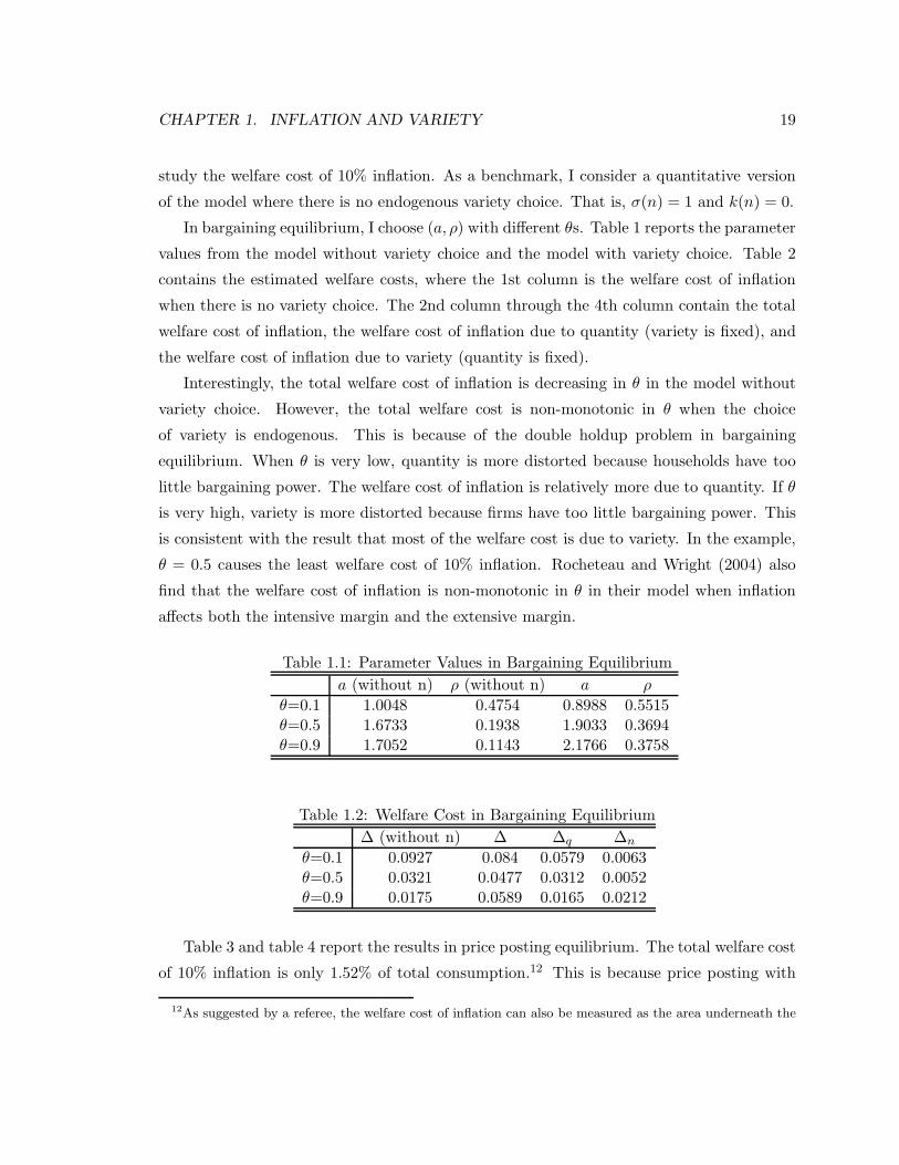
In bargaining equilibrium, I choose (a, ρ) with different θs. Table 1 reports the parameter
values from the model without variety choice and the model with variety choice. Table 2
contains the estimated welfare costs, where the 1st column is the welfare cost of inflation
when there is no variety choice. The 2nd column through the 4th column contain the total
welfare cost of inflation, the welfare cost of inflation due to quantity (variety is fixed), and
the welfare cost of inflation due to variety (quantity is fixed).
Interestingly, the total welfare cost of inflation is decreasing in θ in the model without
variety choice. However, the total welfare cost is non-monotonic in θ when the choice
of variety is endogenous. This is because of the double holdup problem in bargaining
equilibrium. When θ is very low, quantity is more distorted because households have too
little bargaining power. The welfare cost of inflation is relatively more due to quantity. If θ
is very high, variety is more distorted because firms have too little bargaining power. This
is consistent with the result that most of the welfare cost is due to variety. In the example,
θ = 0.5 causes the least welfare cost of 10% inflation. Rocheteau and Wright (2004) also
find that the welfare cost of inflation is non-monotonic in θ in their model when inflation
affects both the intensive margin and the extensive margin.
Table 1.1: Parameter Values in Bargaining Equilibrium
a (without n) ρ (without n) a ρ
θ=0.1 1.0048 0.4754 0.8988 0.5515θ=0.5 1.6733 0.1938 1.9033 0.3694θ=0.9 1.7052 0.1143 2.1766 0.3758
Table 1.2: Welfare Cost in Bargaining Equilibrium
∆ (without n) ∆ ∆q ∆n
θ=0.1 0.0927 0.084 0.0579 0.0063θ=0.5 0.0321 0.0477 0.0312 0.0052θ=0.9 0.0175 0.0589 0.0165 0.0212
Table 3 and table 4 report the results in price posting equilibrium. The total welfare cost
of 10% inflation is only 1.52% of total consumption.12 This is because price posting with
12As suggested by a referee, the welfare cost of inflation can also be measured as the area underneath the
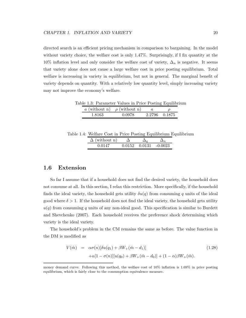
CHAPTER 1. INFLATION AND VARIETY 20
directed search is an efficient pricing mechanism in comparison to bargaining. In the model
without variety choice, the welfare cost is only 1.47%. Surprisingly, if I fix quantity at the
10% inflation level and only consider the welfare cost of variety, ∆n is negative. It seems
that variety alone does not cause a large welfare cost in price posting equilibrium. Total
welfare is increasing in variety in equilibrium, but not in general. The marginal benefit of
variety depends on quantity. With a relatively low quantity level, simply increasing variety
may not improve the economy’s welfare.
Table 1.3: Parameter Values in Price Posting Equilibrium
a (without n) ρ (without n) a ρ
1.8163 0.0978 2.2796 0.1875
Table 1.4: Welfare Cost in Price Posting Equilibrium Equilibrium
∆ (without n) ∆ ∆q ∆n
0.0147 0.0152 0.0131 -0.0023
1.6 Extension
So far I assume that if a household does not find the desired variety, the household does
not consume at all. In this section, I relax this restriction. More specifically, if the household
finds the ideal variety, the household gets utility δu(q) from consuming q units of the ideal
good where δ > 1. If the household does not find the ideal variety, the household gets utility
u(q) from consuming q units of any non-ideal good. This specification is similar to Burdett
and Shevchenko (2007). Each household receives the preference shock determining which
variety is the ideal variety.
The household’s problem in the CM remains the same as before. The value function in
the DM is modified as
V (m) = ασ(n)[δu(q1) + βW+(m − d1)] (1.28)
+α[1 − σ(n)][u(q0) + βW+(m − d0)] + (1 − α)βW+(m).
money demand curve. Following this method, the welfare cost of 10% inflation is 1.69% in price postingequilibrium, which is fairly close to the consumption equivalence measure.
CHAPTER 1. INFLATION AND VARIETY 21
Here (q1, d1) are the terms of trade if the household finds the ideal variety and (q0, d0) are
the terms of trade if the household consumes a non-ideal variety. The probability for a
household to find the ideal variety is ασ(n) and the probability for a household to consume
the non-ideal variety is α[1 − σ(n)]. With probability 1 − α, households are not matched
and consume nothing. The firm’s expected profit becomes
π = maxn
−k(n) + ασ(n)[−c(q1) +1
1 + rφ+d1] + α[1 − σ(n)][−c(q0) +
1
1 + rφ+d0]
.
(1.29)
In the bargaining stage, there are two types of meetings. I use type 1 meeting to refer
to a meeting where a household finds the ideal variety and use type 0 meeting to refer to a
meeting where a household does not find the ideal variety. For a type j, j ∈ 0, 1 meeting,
the generalized Nash problem is
maxqj ,dj
[δju(qj) − βφ+dj ]θ[−c(qj) + βφ+dj ]
1−θ (1.30)
s.t. dj ≤ m,
where δ0 = 1 and δ1 = δ.
One can show that depending on (δ, θ), there are two types of solutions.13 When δ and
θ are not too low and when inflation is not too high, households that find the ideal variety
spend all of the money in the DM. Households that do not find the ideal variety only spend
part of the money and consume the efficient amount of the non-ideal goods. I can prove
that inflation does not affect the consumption of the non-ideal varieties, but it still lowers
the consumption of the ideal varieties. Therefore, inflation lowers expected surplus from
trade and reduces variety. When δ and θ are not too low and when inflation is high, all
households spend all of their money balances. Inflation tends to lower the consumption of
both the ideal varieties and the non-ideal varieties in the DM. When firms receive the same
real balance no matter which goods they sell, the marginal benefit of providing variety comes
from less production associated with producing the ideal variety. Whether inflation reduces
variety depends on whether inflation hurts the consumption of the non-ideal varieties more.
As θ is not too small, it is more likely that inflation hurts the consumption of the non-ideal
varieties more, which implies that the marginal benefit of variety decreases. So inflation can
still reduce variety.
13I only provide a summary of the findings in the extension. Detailed arguments are available upon request.
CHAPTER 1. INFLATION AND VARIETY 22
The other type of solution occurs when δ or θ is too low. All households spend all of their
money balances. Inflation tends to reduce the consumption in the DM. However, when θ is
low enough, inflation might increase variety. The intuition for this result is that inflation
hurts the consumption of the ideal varieties more when θ is very low. As mentioned above,
the marginal benefit of providing the ideal variety is from less production cost. If inflation
hurts the consumption of the ideal varieties more, it implies that the marginal benefit of
variety increases. Inflation may induce firms to increase variety to take advantage of the
lower production. This result is different from the result in the baseline model.
1.7 Conclusion
This paper is motivated by the observation that inflation reduces variety in the market-
place. In a microfounded monetary model, I analyzed the effects of inflation on quantity and
variety. With the two market structures that I considered – bargaining and price posting
with directed search, inflation reduces both quantity and variety.14 While the qualitative
predictions from the two market structures are similar, the quantitative results are quite
different. The welfare cost of inflation due to variety is negligible in price posting equilib-
rium, but it is much bigger in bargaining equilibrium. The paper also studied a theoretical
extension where households are allowed to consume non-ideal varieties. This setup tends to
lower the marginal benefit of variety for firms. As a result, depending on parameter values,
inflation may or may not reduce variety.
There are several extensions of this research that are worth pursuing. First of all, it would
be more desirable to explicitly model product variety following the literature on variety in
international trade. Another extension is to allow free entry by firms. It would be useful
to study how the two types of extensive margins interact when the inflation rate increases.
In this paper, the model predicted that inflation monotonically reduced variety. When
considering Japan in the 1990s and the U.S. in Great Depression, it seems that product
variety also decreased during those deflationary episodes. Inflation and variety might have
an inverse U-shape relationship. This conjecture requires more careful empirical support.
Theoretically, the current model should be modified to study deflation and variety. All these
14For completeness, I also considered Walrasian price taking in the DM. All of the main results remain validwith price taking. The only extra restriction is that c(q) should not be linear. Otherwise, firms always offerthe minimum variety since there is no profit from selling the product. Because I used a linear specificationof c(q) in the quantitative analysis, I did not discuss Walrasian price taking in detail in my paper.
CHAPTER 1. INFLATION AND VARIETY 23
extensions are left for future work.
1.8 Appendix
1.8.1 Proof of Proposition 1.2
Proof. In what follows, I restrict the attention to q ∈ [0, q], where q solves u′(q)g′(q) = 1. For
a household, the choice of m can also be formulated as a choice problem of q, where the
household takes n as given and
maxq
−ig(q) + ασ(n)[u(q) − g(q)] . (1.31)
Recall that the firm takes m as given and chooses n to maximize its expected profit in each
CM. From the Nash bargaining solution, the firm’s problem is equivalent to
maxn
−k(n) + ασ(n)[g(q) − c(q)] . (1.32)
The solution of (q, n) from (1.31) and (1.32) is a Nash equilibrium. Let χ(q;n) be the first
derivative of the objective function in (1.31),
χ(q;n) = −ig′(q) + ασ(n)[u′(q) − g′(q)].
Dividing both sides of the above expression by u′(q), I have
χ(q;n)
u′(q)= ασ(n) − [i + ασ(n)]
g′(q)
u′(q). (1.33)
From assumption 1, the RHS of (1.33) is strictly decreasing in q. As u(q) is strictly concave,1
u′(q) is increasing in q. It follows that χ(q;n) must be decreasing in q, which further implies
that χ′(q;n) < 0. Since χ′(q;n) is the second derivative of (1.31), the household’s objective
function in (1.31) is concave. On the other hand, the firm’s objective function in (1.32) is
also concave because it is immediate to verify that −k′′(n) + ασ′′(n)[g(q) − c(q)] < 0.
Notice that [1] both the household’s objective function in (1.31) and the firm’s objective
function in (1.32) are continuous functions and concave; and [2] I only focus on q ∈ [0, q]
and n ∈ [0, N ]. By the Nash’s Existence Theorem (Ok, p348), the solution of (q, n) to (1.31)
and (1.32) as a Nash equilibrium must exist.
The next step is to establish the existence of a monetary equilibrium under certain
conditions. For q = 0, the household’s objective function in (1.31) is 0 for any n. Simi-
larly, for n = 0, the firm’s objective function in (1.32) is 0 for any q. These two observa-
tions imply that (1.31) and (1.32) should not be negative in any equilibrium. Moreover,
CHAPTER 1. INFLATION AND VARIETY 24
it can be shown that for any q > 0, −ig(q) + ασ(n)[u(q) − g(q)] > 0. As a result, if
maxq
−ig(q) + ασ(n)[u(q) − g(q)] > 0, it implies that the solution of q must not be 0 and
hence q > 0. The only if part of the proposition is obvious. Once q > 0, n > 0 because
g(q) > c(q) (θ = 1 implies that q = n = 0 in equilibrium.) in (1.15).
1.8.2 Proof of Proposition 1.3
Proof. Define f(q; i) = u′(q)g′(q) −1− i
ασ[n(q)] , where n(q) is implicitly defined by (1.15). Notice
that f(q; i) = 0 gives the solution of bargaining equilibrium. As I can show that g′(q) > c′(q),
I know that from (1.15), n(0) = 0 and dndq
> 0. By assumption 1, g′(q)u′′(q)−u′(q)g′′(q)[g′(q)]2
< 0.
From (1.17), dqdn
≥ 0. Also knowing that dndq
> 0, the equilibrium with the highest q is also
the equilibrium with the highest n. Differentiate (1.15) and (1.17) with respect to i,
α[g′(q) − c′(q)]dq
di−
σ′(n)k′′(n) − k′(n)σ′′(n)
[σ′(n)]2dn
di= 0,
g′(q)u′′(q) − u′(q)g′′(q)
[g′(q)]2dq
di+
iσ′(n)
α[σ(n)]2dn
di=
1
ασ(n).
The sign of dndi
is the same as the sign of dqdi
. After rearranging, dqdi
takes the sign of
g′(q)u′′(q) − u′(q)g′′(q)
[g′(q)]2+
iσ′(n)
[σ(n)]2[g′(q) − c′(q)][σ′(n)]2
σ′(n)k′′(n) − k′(n)σ′′(n).
Differentiate f(q; i) with respect to q
f ′(q; i) =g′(q)u′′(q) − u′(q)g′′(q)
[g′(q)]2+
iσ′[n(q)]dndq
ασ[n(q)]2.
When i → 0, limi→0
f ′(q; i) < 0. Recall that q is the solution of u′(q)g′(q) = 1. The solution q to
f(q; i) = 0 must lie between 0 and q. It can be shown that 0 < q ≤ q∗ and n(q) > 0. At
q = q, f(q; i) = − iαbσ[n(q)] < 0 for i > 0. Since q ∈ (0, q) for i > 0, the equilibrium with the
highest q must satisfy f ′(q; i) < 0. Therefore, dqdi
< 0 and dndi
< 0.
1.8.3 Proof of Proposition 1.4
Proof. From (1.17), u′(q) = g′(q) at the Friedman rule. Hence, q is efficient if and only if
g(q) = c(q), which is true when θ = 1. However, the choice of n goes to the corner solution
since from (1.15), −k′(n) < 0. The optimal n is the minimum n. To get the efficient n
from (1.15), one needs g(q) − c(q) = u(q∗) − c(q∗). This is true only when θ = 0 and
CHAPTER 1. INFLATION AND VARIETY 25
q = q∗. However, when θ = 0, monetary equilibrium does not exist. To summarize, it is
not possible to have both efficient q and efficient n in bargaining equilibrium. In (1.15),
g(q) − c(q) < u(q) − c(q) ≤ u(q∗) − c(q∗). Since k′(n)σ′(n) is increasing in n, n < n∗.
In equilibrium, total welfare is increasing in both q and n. As ∂q∂γ
< 0 and ∂n∂γ
< 0 in
equilibrium with the highest (q, n), inflation reduces total welfare. Therefore the Friedman
rule is the optimal monetary policy.
1.8.4 Proof of Lemma 1.5
Proof. I rewrite (1.21) as
maxq,d,Q,n
αf [α−1h (Q)]σ(n)[−c(q) + βφ+d] − k[σ−1(n)]
s.t. − [i + αh(Q)σ(n)]βφ+d + αh(Q)σ(n)u(q) = U ,
and restrict the constraint to the following compact set: Γ(U) = (q, d, n, αh(Q)) ∈ R4, such
that q ∈ [0, q∗], βφ+d ∈ [c(q), u(q)], σ(n) ∈ [0, 1], αh(Q) ∈ [0, 1] and −[i+αh(Q)σ(n)]βφ+d+
αh(Q)σ(n)u(q) ≥ U. Γ(U) is continuous and compact valued correspondence. The objec-
tive function is continuous. By the theorem of the maximum, the set of solutions Υ(U) is
nonempty and upper-hemicontinuous.
1.8.5 Proof of Lemma 1.6
Proof. It is obvious that Q(U ) is nonempty and upper-hemicontinuous from lemma 1.
Define
Ψ(q,Q, n; U ) = αf (Q)σ(n)[−c(q) +αh(Q)σ(n)u(q) − U
i + αh(Q)σ(n)] − k(n).
Consider U1 > U0 > 0.Hence, Υ(U1) = (q1, d1, Q1, n1) and Υ(U0) = (q0, d0, Q0, n0). First
note that when Q0 = 0, it must be true that Q1 = 0. Now considering Q0 > 0, it must
be true that Ψ(q1, Q1, n1; U1) ≥ Ψ(q0, Q0, n0; U1) and Ψ(q0, Q0, n0; U0) ≥ Ψ(q1, Q1, n1; U0)
It implies that Ψ(q1, Q1, n1; U1) − Ψ(q1, Q1, n1; U0) ≥ Ψ(q0, Q0, n0; U1) − Ψ(q0, Q0, n0; U0).
From the definition of Ψ(q,Q, n; U), I have
αf (Q0)σ(n0)
i + αh(Q0)σ(n0)≥
αf (Q1)σ(n1)
i + αh(Q1)σ(n1).
Notice that αf (Q) is increasing in Q, αh(Q) is decreasing in Q and σ(n) is increasing
in n. For (Q0, n0) and (Q1, n1), the only possible cases are: 1) Q0 > Q1 and n0 > n1; 2)
CHAPTER 1. INFLATION AND VARIETY 26
Q0 > Q1 and n0 < n1; 3) Q0 < Q1 and n0 > n1; 4) Q0 > Q1 and n0 = n1; 5) Q0 = Q1 and
n0 > n1; 6) Q0 = Q1 and n0 = n1.
Since U1 > U0 > 0, it must be true that q1 > 0 and q2 > 0 from (1.22). I will show in
the next step that case 3), 5) and 6) can be ruled out. In cases 3), 5) and 6), Q1 ≥ Q0 > 0
and thus it follows that (q0, Q0) and (q1, Q1) should satisfy (1.24) and (1.25). From (1.24),
since u′(q)c′(q) is decreasing in q, αh(Q) is decreasing in Q and σ(n) is increasing in n, q0 > q1
in case 3), 5) and q0 = q1 in case 6). Rearranging (1.25),
u(q) −u′(q)
c′(q)
η(Q)u′(q)c(q) + [1 − η(Q)]c′(q)u(q)
η(Q)u′(q) + [1 − η(Q)]c′(q)=
U
αh(Q)σ(n). (1.34)
Define the LHS of (1.34) as G(q,Q).
G(q,Q) = u(q)
1 −η(Q)u′(q)c(q)
c′(q)u(q) + [1 − η(Q)]
η(Q) + [1 − η(Q)] c′(q)u′(q)
.
By assumption 2 (i) and (ii), I can show that u′(q)c(q)c′(q)u(q) is decreasing in q, which further
implies that ∂G(q,Q)∂q
> 0. By assumption 2, ∂G(q,Q)∂Q
≤ 0. In case 3) and 5), G(q0, Q0) >
G(q1, Q1). In case 6), G(q0, Q0) = G(q1, Q1). Now consider the RHS of (1.34). In case 3)
and 5), U0αh(Q0)σ(n0) < U1
αh(Q1)σ(n1) , which is a contradiction with G(q0, Q0) > G(q1, Q1). In
case 6), U0αh(Q0)σ(n0) < U1
αh(Q1)σ(n1) , which is also a contradiction with G(q0, Q0) = G(q1, Q1).
To summarize, given that U0 < U1, it is only possible that Q0 > Q1. So Q(U) is strictly
decreasing in Q.
1.8.6 Proof of Proposition 1.8
Proof. In equilibrium,∑
ω
Fω = 1,∑
ω
FωQω = 1. It implies that 1 belongs to Q(U ), where
Q(U) is the convex hull of Q(U). Q(U) is convex-valued and upper hemicontinuous. By
lemma 2, Q(U ) is strictly decreasing in U . If Q(0) < 1, the only equilibrium is to have
U = 0. Let Q(0) be the demand for households when U = 0 and it can be solved from
(1.24)-(1.26). When U > u(q∗) − c(q∗), Q(U) = 0 and Q(U ) = 0. Since households are
indifferent whether participating or not, Q = Q(0) and (q, n) solves (1.24) and (1.26). If
Q(0) ≥ 1, Q(U) = 1 determines a unique U because Q(U) is strictly decreasing in U . Note
that the unique U may admit multiple Q. From now on, I focus on symmetric equilibrium.
In a symmetric equilibrium, U determines a unique Q. Notice that U also determines a
CHAPTER 1. INFLATION AND VARIETY 27
unique Q if Q(U) is convex-valued or if Q(U) is a function. Once Q is unique and Q(0) > 1,
Q = 1. To summarize, Q = minQ(0), 1 in equilibrium.
Knowing Q, (1.24) and (1.26) can be used to solve for interior (q, n). From (1.24),dqdn
> 0. Let ϕ(q) = c′(q)[u(q)−c(q)]η(Q)u′(q)+[1−η(Q)] . It is immediate that ϕ′(q) > 0 for q ∈ (0, q∗]. From
(37), dndq
> 0. If there exist multiple solutions of (q, n), these solutions also need to satisfy
(1.25). Since dqdn
> 0 and dndq
> 0, it is not possible to have multiple solutions that satisfy
(1.25). Therefore, (q, n) is also unique. The equilibrium with interior solutions is also
unique.
To focus on monetary equilibrium, one needs to rule out q = n = 0 as a solution. If
Q(0) > 1, Q = 1 and equilibrium U > 0, which implies that q > 0 from (1.22). That is,
monetary equilibrium must exist if Q(0) > 1. If Q(0) ≤ 1, then Q = Q(0) and U = 0
in equilibrium. In this case, if maxq,n
αf (Q)σ(n)[−c(q) + αh(Q)σ(n)u(q)i+αh(Q)σ(n) ] − k(n)
> 0 where
Q = Q(0), q must not be 0 and the solution entails q > 0.
1.8.7 Proof of Proposition 1.9
Proof. Differentiate (1.24) and (1.26) with respect to i,
c′(q)u′′(q) − u′(q)c′′(q)
[c′(q)]2dq
di+
iσ′(n)
αh(Q)[σ(n)]2dn
di=
1
αh(Q)σ(n),
αf (Q)ϕ′(q)dq
di−
σ′(n)k′′(n) − k′(n)σ′′(n)
[σ′(n)]2dn
di= 0.
It follows that dqdi
and dndi
take the same sign. After rearranging, the sign of dqdi
depends on
the sign of
c′(q)u′′(q) − u′(q)c′′(q)
[c′(q)]2+
iσ′(n)
αh(Q)[σ(n)]2αf (Q)ϕ′(q)[σ′(n)]2
σ′(n)k′′(n) − k′(n)σ′′(n).
Let f(q; i) = u′(q)c′(q) − 1 − i
αh(Q)σ[n(q)] , where n(q) is implicitly defined by (1.26). The
solution of q is given by f(q; i) = 0. Differentiate f(q; i) with respect to q:
f ′(q; i) =c′(q)u′′(q) − u′(q)c′′(q)
[c′(q)]2+
iσ′(n)
αh(Q)[σ(n)]2dn
dq.
At q = q∗, f(q∗; i) = − iαh(Q)σ[n(q∗)] ≤ 0. Since I restrict the solution to q ∈ (0, q∗], it implies
that f ′(q; i) < 0 when f(q; i) = 0 for q ∈ (0, q∗). As the solution of q converges to q∗ only
at i → 0, limi→0
f ′(q∗; 0) = c′(q∗)u′′(q∗)−u′(q∗)c′′(q∗)[c′(q∗)]2
< 0. For solution q ∈ (0, q∗], f ′(q; i) < 0.
Therefore, dqdi
< 0 and furthermore, dndi
< 0. It is equivalent to conclude that dqdγ
< 0 anddndγ
< 0.
CHAPTER 1. INFLATION AND VARIETY 28
1.8.8 Proof of Proposition 1.10
Proof. From (1.24), q is efficient when i → 0. The Friedman rule achieves the efficient q.
For n, as long as q is efficient, n is also efficient. When i > 0, (1.24) implies that q < q∗. Since
u′(q) > c′(q) and u(q)− c(q) < u(q∗)− c(q∗) for q ∈ (0, q∗), ϕ(q)[u(q)− c(q)] < u(q∗)− c(q∗).
Because k′(n)σ′(n) is increasing in n, in general n < n∗.
1.9 References
Acemoglu, Daron and Robert Shimer, ”Holdups and Efficiency with Search Frictions,” In-
ternational Economic Review, Vol. 40 (1999), pp. 827-849.
Aruoba, Boragan, Guillaume Rocheteau and Christopher J. Waller, ”Bargaining and the
Value of Money,” Journal of Monetary Economics, Vol. 54 (2007), pp. 2636-2655.
Broda, Christian and David Weinstein, ”Globalization and the Gains from Variety”, Quar-
terly Journal of Economics, Vol. 121 (2006), pp. 541-585.
Burdett, Ken and Andrei Shevchenko, ”Money and the Variety of Goods,” manuscript,
Michigan State University, 2007.
Burdett, Ken, Shouyong Shi and Randall Wright, ”Pricing and Matching with Frictions,”
Journal of Political Economy, Vol. 109 (2001), pp. 1060-1085.
Camera, Gabriele, Robert R. Reed and Christopher J. Waller, ”Jack of All Traders or a
Master of One? Specialization, Trade, and Money,” International Economic Review,
Vol. 44 (2003), pp. 1275-1294.
CCR, ”Evolucion de la Cantidad de SKUs Vendidos Antes y Despues de la Devaluacion en
las Cadenas de Hipermercados, Supermercados y Hard Discounts en la Argentina”,
2003.
Corbae, Dean and Borghan Narajabad, ”A Hotelling Model with Money,” manuscript, The
University of Texas at Austin, 2007.
Craig, Ben and Guillaume Rocheteau, ”Inflation and Welfare: A Search Approach,” Journal
of Money, Credit, and Banking, Vol. 40 (2008), pp. 89-119.
CHAPTER 1. INFLATION AND VARIETY 29
Ghossoub, Edgar and Robert R. Reed, ”Money and Specialization in a Neoclassical Growth
Model,” Journal of Money, Credit, and Banking, Vol. 37 (2005), pp. 969-975.
Guardiano, John, ”Exploding the Myth about Economic Reform in Russia,” Backgrounder
#930, The Heritage Foundation, 1993.
Guttmann, William and Patricia Meehan, The Great Inflation, Germany 1919-23 (Farnbor-
ough, Eng.: Saxon House, 1975).
Heymann, Daniel and Axel Leijonhufvud, High Inflation (Oxford University Press, 1995).
International Herald Tribune, ”Inflation in Zimbabwe Surges to Record 3714 Percent, the
Highest in the World”, the Associate Press, May 17th, 2007.
Kiyotaki, Nobuhiro and Randall Wright, ”A Search-Theoretic Approach to Monetary Eco-
nomics,” American Economic Review, Vol. 83 (1993), pp. 63-77.
Lagos, Ricardo and Guillaume Rocheteau, ”Inflation, Output, and Welfare,” International
Economic Review, Vol. 46 (2005), pp. 495-522.
Lagos, Ricardo and Randall Wright, ”A Unified Framework for Monetary Theory and Policy
Analysis,” Journal of Political Economy, Vol. 113 (2005), pp. 463-484.
Laing, Derek, Victor Li and Ping Wang, ”Inflation and Productive Activity in a Multiple-
Matching Model of Money,” Journal of Monetary Economics, 54 (2007), pp. 1949-
1961.
Lancaster, Kelvin, ”The Economics of Product Variety: A Survey,” Marketing Science, 9
(1990), 189-206.
Lucas, Robert E., ”Inflation and Welfare,” Econometrica, Vol. 68 (2000), pp. 247-274.
McKenzie, David and Ernesto Schargrodsky, ”Buying Less, but Shopping More: the Use of
Non-Market Labor During a Crisis,” BREAD Working Paper, No. 92, 2006.
Midrigan, Virgiliu, ”Comments on Monetary Policy and Business Cycle with Endogenous
Entry and Product Variety by Bilbiie, Ghironi and Metlitz,” manuscript, New York
University, 2007.
CHAPTER 1. INFLATION AND VARIETY 30
Moen, Espen, ”Competitive Search Equilibrium,” Journal of Political Economy, Vol. 105
(1997), pp. 385-411.
Ok. Efe A., Real Analysis with Economic Applications (Princeton and Oxford: Princeton
University Press, 2007).
Rocheteau, Guillaume and Randall Wright, ”Inflation and Welfare in Models with Trading
Frictions,” in D. Altig and E. Nosal, eds., Monetary Policy in Low Inflation Economies
(Cambridge University Press, forthcoming).
Rocheteau, Guillaume and Randall Wright, ”Money in Search Equilibrium, in Competitive
Equilibrium and in Competitive Search Equilibrium,” Econometrica, Vol. 73 (2005),
pp. 175-202.
Shevchenko, Andrei, ”Middleman,” International Economic Review, Vol. 45 (2004), pp.
1-24.
Shi, Shouyong, ”Money and Specialization,” Economic Theory, Vol. 10 (1997), pp. 99-113.
White, Lawrence J., ”Market Structure and Product Varieties,” American Economic Review,
Vol. 67 (1977), pp. 179-182.
Chapter 2
Money and Costly Credit1
2.1 Introduction
This paper develops a model of money and credit in order to study issues in monetary
economics concerning the choice of payment methods and the effects of inflation. Not
too long ago, consumers typically paid for things using either cash or checks. A check is
essentially an IOU for a future cash payment; to be drawn from the consumer’s bank account
and credited to the merchant’s bank account. In recent decades, the payment instruments
available to consumers have expanded to include debit and credit cards. A debit transaction
is essentially the electronic equivalent of a cash transaction. A credit transaction in some
ways resembles a check transaction; except that the credit is now offered by some third party
(rather than the merchant), with this third party willing to postpone debt settlement to the
indefinite future (typically at very high rates of interest). The key difference between credit
and the other forms of means of payment is that the acquisition of money is not necessary
to make a purchase using credit, whereas money must be acquired prior to purchasing with
the other forms of means of payment.2 In some sense, credit transactions are settled ”later”,
while transactions using the other means of payment are settled ”now”.
1I would like to thank David Andolfatto and Fernando Martin for many discussions and comments. I alsothank Jonathan Chiu, Geoffrey Dunbar, Hua Jiang, Alex Karaivanov, Daniel Monte, Irina Telyukova, RandyWright and seminar participants at Simon Fraser University, the Summer Workshop on Money, Banking andPayments at the Federal Reserve Bank of Chicago, the Federal Reserve Bank of Cleveland and the Bank ofCanada for helpful suggestions.
2Checks can be viewed as a short-term form credit. Since the time until settlement is typically very shortfor checks, checks are more like cash or debit cards although postal checks resemble credit cards from ahistorical perspective.
31
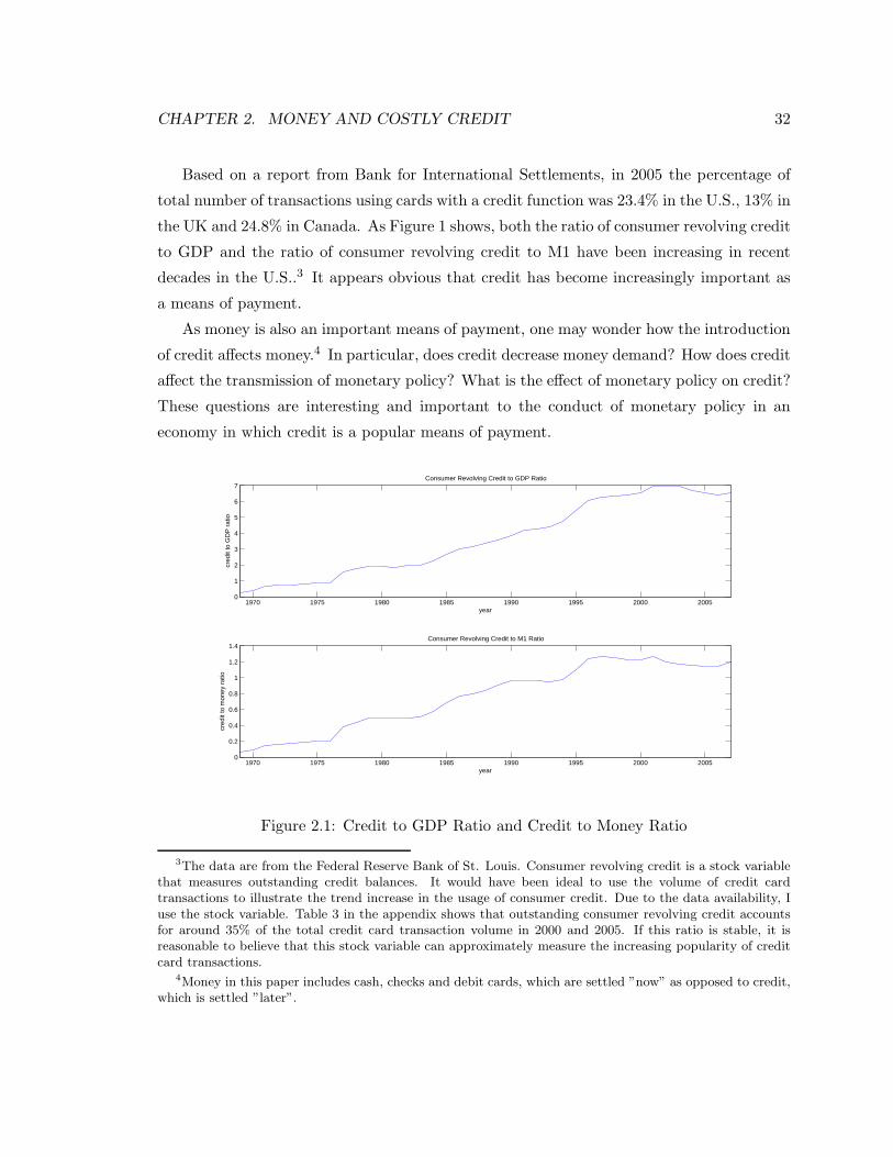
CHAPTER 2. MONEY AND COSTLY CREDIT 32
Based on a report from Bank for International Settlements, in 2005 the percentage of
total number of transactions using cards with a credit function was 23.4% in the U.S., 13% in
the UK and 24.8% in Canada. As Figure 1 shows, both the ratio of consumer revolving credit
to GDP and the ratio of consumer revolving credit to M1 have been increasing in recent
decades in the U.S..3 It appears obvious that credit has become increasingly important as
a means of payment.
As money is also an important means of payment, one may wonder how the introduction
of credit affects money.4 In particular, does credit decrease money demand? How does credit
affect the transmission of monetary policy? What is the effect of monetary policy on credit?
These questions are interesting and important to the conduct of monetary policy in an
economy in which credit is a popular means of payment.
1970 1975 1980 1985 1990 1995 2000 20050
1
2
3
4
5
6
7Consumer Revolving Credit to GDP Ratio
year
cred
it to
GD
P r
atio
1970 1975 1980 1985 1990 1995 2000 20050
0.2
0.4
0.6
0.8
1
1.2
1.4Consumer Revolving Credit to M1 Ratio
year
cred
it to
mon
ey r
atio
Figure 2.1: Credit to GDP Ratio and Credit to Money Ratio
3The data are from the Federal Reserve Bank of St. Louis. Consumer revolving credit is a stock variablethat measures outstanding credit balances. It would have been ideal to use the volume of credit cardtransactions to illustrate the trend increase in the usage of consumer credit. Due to the data availability, Iuse the stock variable. Table 3 in the appendix shows that outstanding consumer revolving credit accountsfor around 35% of the total credit card transaction volume in 2000 and 2005. If this ratio is stable, it isreasonable to believe that this stock variable can approximately measure the increasing popularity of creditcard transactions.
4Money in this paper includes cash, checks and debit cards, which are settled ”now” as opposed to credit,which is settled ”later”.
CHAPTER 2. MONEY AND COSTLY CREDIT 33
It seems clear enough that technological advances in electronic record-keeping have facil-
itated the use of consumer credit. Specialized intermediaries are now able to offer consumer
credit balances with limits that can vary with each person’s recorded credit history. These
technological advances allow credit to substitute for money as a means of payment. Indeed,
this appears to be supported by the evidence. For example, Duca and Whitesell (1995)
estimate based on U.S. household-level data that for every 10% increase in the probability
of owning a credit card, checking balances are reduced by 9%.
The evidence on how inflation affects the money-credit margin is less clear. Empirical
investigation here is hampered to some extent by data limitations and the recent secular im-
provements in credit card technology. Nevertheless, the evidence from various high-inflation
episodes suggests that high inflation hampers the use of credit as a means of payment.
Credit cards gained widespread popularity in Brazil following the successful reduction of
inflation to sustainable levels, with the number of cards in force growing by 88% between
2000 and 2004. In Colombia, because of lower inflation and lending rates, the proportion
of households with formal access to credit was expected to increase by 25% from 2004 to
2008. High inflation episodes also delayed the adoption and widespread use of credit cards
in Turkey. Even in Australia, households’ debts increased dramatically due to the lower
inflation rates and thus lower cost of borrowing during the 1990s.5 Reducing the inflation
rate is perceived to promote the use of credit.
Other empirical evidence regarding the relationship between inflation and credit is based
on a broader measure of credit – namely the ratio of total private credit to GDP.6 Using
a sample of 97 countries, Boyd et al. (2001) conclude that inflation has a negative impact
on credit. See also Boyd and Champ (2003). Later, Khan et al. (2006) also use a large
cross-country sample, but they find that there is a threshold effect of inflation on credit.
Inflation has a negative impact on credit when it exceeds a threshold. The evidence based
on total private credit suggests that inflation tends to have a negative impact on credit at
high rates, but not at low rates.
In this paper, I propose a model that is able to replicate the evidence on inflation,
5The inflation rate was on average around 8% in Australia in the 1980s and was reduced to around 3%in the 1990s.
6Total private credit may be too broad in comparison to consumer credit. Given that [1] it is difficult toobtain data on consumer credit for a large sample of countries over an adequately long time span; and [2]different measures of credit tend to highly comove, as can be seen from the U.S. data, it seems useful andreasonable to review this evidence.
CHAPTER 2. MONEY AND COSTLY CREDIT 34
money demand and credit. The model is built on Lagos and Wright (2005). In monetary
theory, frictions that render money essential make credit arrangements impossible. In order
for credit to exist, I assume that there exist competitive financial intermediaries that can
identify agents and have access to a record-keeping technology. There are two frictions
associated with credit arrangements. First, arranging credit is costly. In a bilateral trade, if
a buyer wants to use credit, he must incur a fixed utility cost in order to make the seller and
himself identified to a financial intermediary. When buyers have heterogeneous preferences,
the fixed cost of credit will endogenously determine the fraction of buyers using credit.
Second, the settlement of credit is available only at a particular time in each period, during
which the financial intermediaries accept repayment of credit and settle debts. Due to the
timing structure of the model, settlement is ”delayed” and money becomes the only means
of settlement.
These two features of the model allow some interesting interactions between money and
credit. Inflation tends to increase the fraction of buyers using credit at low inflation rates,
but decrease the fraction of buyers using credit at high inflation rates. Compared to an
economy without credit, the model has three implications: [1] the real demand for money is
lower at low to moderate inflation rates; [2] social welfare is higher when the inflation rate
exceeds a specific threshold; and [3] for a given inflation rate, the welfare cost of inflation
can be higher for some reasonable values of the credit cost parameter.
Several recent papers have attempted to allow the coexistence of money and credit.7 In
general, some imperfections associated with credit should be incorporated to sustain the
essentiality of money and permit the existence of credit. Sanches and Williamson (2008)
adopt the notion of limited participation in the sense that only an exogenous subset of agents
can use credit. While the banks in Berentsen et al. (2007) can record financial history, they
cannot record goods transaction history so that credit takes the form of bank loans and
bank loans must be taken in the form of fiat money. Telyukova and Wright (2008) build a
model where agents can use money and credit to explain the credit card debt puzzle. Their
market structure determines that agents do not use money and credit simultaneously. A
more related paper is Chiu and Meh (2008). They study how banks as in Berentsen et al.
7The literature on money and credit is vast and thus I cannot hope to review it in its totality. Rather, Iwill only mention a few papers that are more recent or are more or less directly related to this paper. Forexample, for recent attempts to rationalize the coexistence of inside and outside money, see Cavalcanti andWallace (1998), Kocherlakota and Wallace (1998), Mills (2007), Sun (2007). A more recent paper by Lesteret al. (2008) studies the coexistence of multiple assets which differ in their return and liquidity.
CHAPTER 2. MONEY AND COSTLY CREDIT 35
(2007) affect allocations and welfare in an economy where ideas (or projects) are traded
among investors and heterogeneous entrepreneurs. The role of banking is similar to credit,
but money is the only means of payment in their paper. In this paper, both money and
credit can serve as means of payment, and the choice of payment methods is endogenous.
In terms of the model’s prediction on inflation and credit, the paper’s result is similar
to the result of Azariadis and Smith (1996). The key friction for their result is asymmetric
information associated with using credit. This paper instead considers different frictions
that affect the use of credit. Several papers have used the notion of costly credit in the
Cash-in-Advance model or in the OLG model.8 With the fixed cost, it is not surprising that
inflation always decreases money demand and increases credit demand. I label the effect
of inflation on credit through the fixed cost channel as the fixed cost effect. The ”delayed”
settlement has been used in Ferraris (2006), where money and credit are complements. In
fact, this idea can be traced back to Stockman (1981), where he shows that inflation reduces
the capital stock if money and capital are complements. The delayed settlement effect of
inflation on credit is that inflation should reduce credit. As credit is subject to both frictions
in this paper, it turns out that the fixed cost effect dominates at low inflation rates and
the delayed settlement effect dominates at high inflation rates. This prediction is consistent
with the empirical evidence cited above.
The rest of the paper is organized as follows. Section 2 lays out the physical environment.
Section 3 solves for the equilibrium and analyzes the equilibrium when the repayment of
credit can be enforced. I numerically study the model in Section 4. In Section 5, I consider
monetary equilibrium when the repayment of credit cannot be enforced. Finally, Section 6
concludes. All proofs are provided in the Appendix.
2.2 Environment
Time is discrete and runs forever. In each period, there are three submarkets that open
sequentially. The first submarket is characterized by bilateral trades and is labelled as
market 1. The second submarket is characterized by a centrally located competitive spot
market and is labelled as market 2. No trade occurs in the third submarket and it is labelled
as market 3. The activity in the third submarket will be described in detail later. There
8For Cash-in-Advance models, see Lacker and Shreft (1996), Aiyagari et al. (1998), and English (1999)for examples. For the OLG framework, see Freeman and Huffman (1991) for an example.
CHAPTER 2. MONEY AND COSTLY CREDIT 36
are two permanent types of agents – buyers and sellers, each with measure 1. Buyers are
those who want to consume in market 1 and sellers are those who produce in market 1. All
agents are anonymous and lack commitment. Each buyer receives a preference shock ε at
the beginning of each period, which determines the buyer’s preference in market 1.9 The
preference shock ε is drawn from a c.d.f. G(ε). The preference shocks are iid across buyers
and across time. The realization of these preference shocks is public information. There are
two types of goods. Goods that are produced and consumed in market 1(2) are called good
1(2). All goods are nonstorable.
In market 1, buyers and sellers are matched randomly according to a matching tech-
nology. The probability that a buyer (seller) meets a seller (buyer) is σ with 0 < σ ≤ 1.
Given that a buyer and a seller meet, the terms of trade are determined by the buyer’s
take-it-or-leave-it offer. After exiting market 1, all agents enter market 2. Buyers supply
labor for production and consume good 2. Sellers only consume good 2. For simplicity, the
production technology in market 2 is assumed to be linear and 1 unit labor can be converted
into 1 unit of good 2.
The preference of a buyer with a preference shock ε is εu(q) + v(x) − h, where εu(q) is
the buyer’s utility from consuming q units of good 1. As usual, u(0) = 0, u′(0) = ∞ and
u′′(q) < 0 < u′(q). In market 2, the buyer’s utility from consuming x units of good 2 is v(x),
where limx→0 υ′(x) = ∞ and υ′′(x) < 0 < υ′(x). The buyer’s disutility from working is h.
The preference of a seller is −c(q) + y, where c(q) is the seller’s disutility from producing
q units of good 1 with c(0) = 0, c′(0) = 0, c′(q) > 0 and c′′(q) ≥ 0. The seller has a linear
utility in market 2, where y is the amount of consumption of good 2. All agents discount
between market 3 and the next market 1. The discount rate is β.
Now I consider a planner’s problem as the benchmark allocation. Suppose that the
planner weights all agents equally and is subject to the random matching technology. I
restrict the attention to stationary allocations in what follows. In market 1 of each period,
given a buyer’s preference shock ε and the buyer meeting a seller, the planner instructs the
seller to produce q(ε) for the buyer. Those agents who do not find a match consume and
produce nothing. In market 2 of each period, the planner assigns the consumption of good
2 x, y and the labor supply h subject to the resource constraint. Formally, the planner’s
9There are a variety of ways to model the heterogeneity in this model. For example, one can modelheterogeneous sellers that have different cost functions or model heterogeneity as match specific shocks.
CHAPTER 2. MONEY AND COSTLY CREDIT 37
problem is
maxq(ε),x,y,h
σ
∫
[εu(q(ε)) − c(q(ε))]dG(ε) + υ(x) − h + y
(2.1)
s.t. x + y = h.
The optimal (x∗, q∗(ε)) are characterized by υ′(x) = 1 and εu′(q(ε)) = c′(q(ε)) for all ε.
The optimal q(ε) is increasing in ε. In fact, the optimal allocation features a slight indeter-
minacy. That is, given the quasi-linear preference structure, h and y are indeterminate as
long as h − y = x∗.
The planner’s allocation cannot be implemented in the economy since agents are anony-
mous and lack commitment. As a result, bilateral trade credit is not possible and thus
money is essential. I assume that there exists a monetary authority that controls the supply
of money. Let M denote the aggregate money supply at any given date. It grows at a
gross rate γ > 0, i.e., M = γM . Here the hat denotes the variable in the next period. I
will consider γ > β and γ → β from above. New money is injected (or withdrawn) via a
lump-sum transfer (or tax) to each buyer at the beginning of each period and the transfer
is τ = (γ − 1)M.
Besides the monetary authority, there exist competitive financial intermediaries. These
financial intermediaries possess a record-keeping technology, which allows them to identify
agents and keep track of goods market transaction history. Clearly the availability of the
record-keeping technology makes credit arrangements through the financial intermediaries
possible in this economy. To sustain the essentiality of money, I assume two frictions as-
sociated with the record-keeping technology. The first friction is that the record-keeping
technology or the financial intermediaries are not available in market 2. This restriction im-
plies that agents may arrange credit transactions in market 1, but cannot settle their debts
in market 2. As the financial intermediaries are available in market 3, buyers who have used
credit in market 1 repay their debts and sellers who have extended credit get repayment
in market 3. One can think of market 3 as an overnight market for settlement. Without
such a restriction, agents would want to settle their debts in market 2. In some sense, the
settlement of debts is delayed. Since goods are nonstorable, money becomes the only means
of settlement. The second friction associated with the record-keeping technology is that it
is costly. As all agents are anonymous, the buyer in a match in market 1 can incur a fixed
utility cost k to make the pair identifiable to a financial intermediary so that the seller can
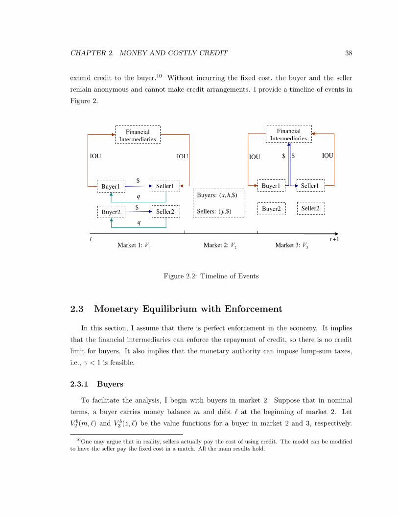
CHAPTER 2. MONEY AND COSTLY CREDIT 38
extend credit to the buyer.10 Without incurring the fixed cost, the buyer and the seller
remain anonymous and cannot make credit arrangements. I provide a timeline of events in
Figure 2.
t +1t
$$ IOUIOU
q
$
$
q
IOU IOU
FinancialIntermediaries
Buyer1 Seller1
Buyer2 Seller2
FinancialIntermediaries
Buyer1 Seller1
Buyer2 Seller2
Buyers: ,$),( hx
Sellers: ,$)(y
Market 2: 2VMarket 1: 1V Market 3: 3V
Figure 2.2: Timeline of Events
2.3 Monetary Equilibrium with Enforcement
In this section, I assume that there is perfect enforcement in the economy. It implies
that the financial intermediaries can enforce the repayment of credit, so there is no credit
limit for buyers. It also implies that the monetary authority can impose lump-sum taxes,
i.e., γ < 1 is feasible.
2.3.1 Buyers
To facilitate the analysis, I begin with buyers in market 2. Suppose that in nominal
terms, a buyer carries money balance m and debt ℓ at the beginning of market 2. Let
V b2 (m, ℓ) and V b
3 (z, ℓ) be the value functions for a buyer in market 2 and 3, respectively.
10One may argue that in reality, sellers actually pay the cost of using credit. The model can be modifiedto have the seller pay the fixed cost in a match. All the main results hold.
CHAPTER 2. MONEY AND COSTLY CREDIT 39
Notice that the buyer cannot pay off his debt in market 2 because the financial intermediaries
are not available. However, the buyer can accumulate money balance. Let z denote the
money balance that the buyer carries to market 3. The buyer’s choice problem is
V b2 (m, ℓ) = max
x,h,z
v(x) − h + V b3 (z, ℓ)
(2.2)
s.t. x + φz = φm + h,
where φ is the inverse of the price level (or the value of money). Substituting h from the
buyer’s budget constraint into (2.2), the unconstrained problem is
V b2 (m, ℓ) = φm + max
x,zv(x) − x − φz + V b
3 (z, ℓ).
The first order conditions for interior solutions are v′(x) = 1 and
∂V b3 (z, ℓ)
∂z= φ. (2.3)
As is standard, the choice of z does not depend on m; however, it depends on ℓ. Intuitively,
if the buyer incurs more debt in market 1, he must accumulate more money in market 2 for
repayment in market 3. The envelope conditions imply
∂V b2 (m, ℓ)
∂m= φ, (2.4)
∂V b2 (m, ℓ)
∂ℓ=
∂V b3 (z, ℓ)
∂ℓ. (2.5)
Note that V b2 (m, ℓ) is linear in m.
For the buyer entering market 3, the value function is
V b3 (z, ℓ) = β
∫
V b1 (z − ℓ + τ , 0; ε)dG(ε).
The only activity for the buyer in market 3 is to repay his debt. Due to the quasilinear
structure of the buyer’s preference, the buyer should be indifferent between repaying the
debt in the current market 3 or in any future market 3. I assume that if the buyer has
any debt, he repays in the current market 3. To simplify notations, let m = z − ℓ + τ be
the buyer’s money holding at the beginning of the next period. For a buyer receiving a
preference shock ε at the beginning of the next period, let V b1 (m, 0; ε) be the buyer’s value
function. Since V b1 (m, 0; ε) depends on ε, I take the expected value for the buyer in market
CHAPTER 2. MONEY AND COSTLY CREDIT 40
3 and discount it by β. The envelope conditions yield
∂V b3 (z, ℓ)
∂z= β
∫
∂V b1 (m, 0; ε)
∂mdG(ε), (2.6)
∂V b3 (z, ℓ)
∂ℓ= −β
∫
∂V b1 (m, 0; ε)
∂mdG(ε). (2.7)
Combining (2.3) and (2.5) with (2.6) and (2.7),
∂V b3 (z, ℓ)
∂z= β
∫
∂V b1 (m, 0; ε)
∂mdG(ε) = −
∂V b3 (z, ℓ)
∂ℓ= −
∂V b2 (m, ℓ)
∂ℓ= φ. (2.8)
From (2.8), V b2 (m, ℓ) is linear in ℓ and V b
2 (m, ℓ) = φm − φℓ + V b2 (0, 0).
After exiting market 3, each buyer realizes a preference shock ε. For a buyer with ε, the
value function in market 1 is
V b1 (m, 0; ε) = σ[εu(q) − k · I(a) + V b
2 (m − d, a · I(a))] + (1 − σ)V b2 (m, 0),
where (q, d, a) are the terms of trade. With probability σ, the buyer spends d units of money
and uses a units of credit in nominal terms in exchange for q units of good 1 from the seller.
An indicator function I(a) is such that I(a) = 1 if a > 0 and I(a) = 0 if a = 0. With
probability 1 − σ, the buyer is not matched and carries his money to market 2.
2.3.2 Sellers
Let V s2 (m, ℓ) and V s
3 (z, ℓ) be a seller’s value functions in market 2 and 3, respectively.
Since the seller is the creditor, ℓ should be either 0 or negative. The seller’s value function
in market 2 is
V s2 (m, ℓ) = max
y,zy + V s
3 (z, ℓ) (2.9)
s.t. y + φz = φm.
By substituting y from the constraint into (2.9), the first order condition of the unconstrained
problem is∂V s
3 (z, ℓ)
∂z≤ φ, and z = 0 if
∂V s3 (z, ℓ)
∂z< φ. (2.10)
The envelope conditions yield
∂V s2 (m, ℓ)
∂m= φ, (2.11)
∂V s2 (m, ℓ)
∂ℓ=
∂V s3 (z, ℓ)
∂ℓ. (2.12)
CHAPTER 2. MONEY AND COSTLY CREDIT 41
Again, V s2 (m, ℓ) is linear in m.
For the seller in market 3, the value function is
V s3 (z, ℓ) = β
∫
V s1 (z − ℓ, 0; ε)dG(ε).
If the seller has extended any credit in the previous market 1, the seller will receive repayment
from the financial intermediary in market 3. I take the expected value function of the seller
because the seller anticipates that a potential buyer he will meet in the next market 1 may
have a preference shock ε drawn from G(ε). Let m = z−ℓ denote the seller’s money holding
at the beginning of the next market 1. The envelope conditions are
∂V s3 (z, ℓ)
∂z= β
∫
∂V s1 (m, 0; ε)
∂mdG(ε), (2.13)
∂V s3 (z, ℓ)
∂ℓ= −β
∫
∂V s1 (m, 0; ε)
∂mdG(ε). (2.14)
Now combining (2.12) with (2.13) and (2.14), I obtain
∂V s3 (z, ℓ)
∂z= β
∫
∂V s1 (m, 0; ε)
∂mdG(ε) = −
∂V s3 (z, ℓ)
∂ℓ= −
∂V s2 (m, ℓ)
∂ℓ. (2.15)
For the seller who potentially meets a buyer with ε, the value function in market 1 is
V s1 (m, 0; ε) = σ[−c(q) + V s
2 (m + d,−a)] + (1 − σ)V s2 (m, 0). (2.16)
If the seller meets a buyer, the seller sells q units of good 1, receives d units of money and
extends credit with the nominal value a if the buyer chooses to use credit.
2.3.3 Equilibrium
Take-it-or-Leave-it Offer
Before deriving the equilibrium conditions, I solve for the terms of trade in market 1.
The terms of trade in a match are determined by the buyer’s take-it-or-leave-it offer.11
There are two types of trades in market 1, depending on whether the buyer in a match uses
credit or not.
11It will be interesting to generalize the buyer’s bargaining power from 1 to less than 1. It will also beinteresting to study other pricing mechanisms that have been used in the literature such as competitivepricing and price posting. In this paper, I only focus on the buyer’s take-it-or-leave-it offer to get the mainintuition from the model and leave those extensions for future work.
CHAPTER 2. MONEY AND COSTLY CREDIT 42
Suppose that a buyer with ε only uses money. Recall that V b1 and V s
1 are linear in m.
The buyer’s problem is
maxq,d
[εu(q) − φd]
s.t. c(q) = φd and d ≤ m,
where m is the buyer’s money holding. Let λ1 and λ2 be the Lagrangian multipliers asso-
ciated with the two constraints.
L = maxq,d,λ1,λ2
[εu(q) − φd] + λ1[φd − c(q)] + λ2(m − d).
It is straightforward that the solution is the following.
λ2 = 0 : (q, d) are given by εu′(q) = c′(q) and φd = c(q),
λ2 > 0 : (q, d) are given by d = m and c(q) = φd.
Suppose that the buyer with ε uses credit. From (2.8), V b2 is also linear in ℓ. However,
it is not clear that V s2 must be linear in ℓ at this stage. So I define the buyer’s problem as
maxq,d,a
[εu(q) − k − φd − φa]
s.t. c(q) = φd + V s2 (0,−a) − V s
2 (0, 0) and d ≤ m.
It is obvious that the seller’s money holding does not appear in the above problem. There-
fore, the terms of trade with credit do not depend on the seller’s money holding. In addition,
recall that the terms of trade without credit do not depend on the seller’s money holding.
It follows from (2.16) that
∂V s1 (m, 0; ε)
∂m= σφ + (1 − σ)φ = φ. (2.17)
From (2.15) and (2.17),
∂V s3 (z, ℓ)
∂z= −
∂V s3 (z, ℓ)
∂ℓ= −
∂V s2 (m, ℓ)
∂ℓ= βφ. (2.18)
Two results follow from (2.18). First, V s2 is linear in ℓ and V s
2 (m, ℓ) = φm−βφℓ + V s2 (0, 0).
Second, sellers choose z = 0. One can show that the gross inflation rate is φ
φ= γ in the
steady state. As I only consider γ > β and γ → β from above, the second result is derived
from (2.10) and (2.18).
CHAPTER 2. MONEY AND COSTLY CREDIT 43
Using (2.18), the Lagrangian is
L = maxq,d,a,λ1,λ2
[εu(q) − k − φd − φa] + λ1[φd + βφa − c(q)] + λ2(m − d).
It turns out that the inequality constraint is always binding, and thus d = m. The solutions
for (q, a) are
εu′(q) =γ
βc′(q), (2.19)
βφa = c(q) − φd. (2.20)
It is interesting to note that q depends on γ. In this economy, if a buyer uses credit in market
1, he will accumulate money for debt repayment in market 2. However, for the seller who
extends the credit in the match, he will not be paid in the same market 2. Instead, the seller
must wait to get settled in market 3. After receiving the money, the seller carries the money
to the next market 1, but he cannot spend it because he does not want to consume. Hence,
the seller actually spends the money one period after the buyer accumulates the money.
There is an asymmetry between the time at which the buyer accumulates the money for
repayment and the time at which the seller can spend the money from repayment. The
buyer must compensate the seller for the loss in the value of money. From (2.20), the buyer
essentially borrows βφφ
a and repays a in nominal terms. The nominal interest rate of credit
is 1 + i = φ
βφ= γ
β. As γ is higher, credit is more costly in nominal terms. For any given ε,
q is decreasing in γ. Credit transactions are subject to inflation distortion.
As the structure of the model implies that money is the only means to settle credit, one
may think that it is natural inflation affects a credit transaction’s terms of trade. However,
this is not necessarily true. The key feature that makes credit subject to inflation distortion
is the inability of sellers to spend the money from repayment right away. Imagine an
environment in which financial intermediaries exist in market 2 and the settlement of credit
requires money. Sellers receive the repayment in the form of money and can spend it in
market 2. It is clear that a credit transaction’s terms of trade do not depend on the inflation
rate in this scenario although money is imposed as the only means of settlement.
Money versus Credit
Having solved the terms of trade, I proceed to find the condition that determines whether
a buyer uses credit or not. For a buyer with ε in market 1, if he only uses money,
V b1 (m, 0; ε) = σ[εu(q) − c(q)] + φm + V b
2 (0, 0).
CHAPTER 2. MONEY AND COSTLY CREDIT 44
If the buyer uses credit,
V b1 (m, 0; ε) = σ[εu(q) −
γ
βc(q) + (
γ
β− 1)φm − k] + φm + V b
2 (0, 0).
Let T (ε) be the net benefit of using credit for the buyer, where
T (ε) = σ[εu(qc) −γ
βc(qc) + (
γ
β− 1)φm − k] − σ[εu(qm) − c(qm)]. (2.21)
I use qc to denote the quantity traded with credit and qm to denote the quantity traded
without credit. For the rest of the paper, I assume that ε is uniformly distributed, ε ∼
U(0, 1].
Lemma 2.1 For any given inflation rate γ, there exist two threshold values of ε, ε0 and ε1
such that
0 ≤ ε ≤ ε0, the buyer spends d < m, a = 0 and consumes q∗ where εu′(q∗) = c′(q∗),
ε0 ≤ ε ≤ ε1, the buyer spends d = m, a = 0 and consumes q where c(q) = φm,
ε1 ≤ ε ≤ 1, the buyer spends d = m, a > 0 and consumes qc where εu′(qc) = γβc′(qc).
Lemma 1 is very intuitive. If a buyer receives a very low ε, he has enough money at hand
to afford q∗, which is the optimal consumption for him. Here ε0 is the threshold that deter-
mines whether a buyer is liquidity constrained. For a buyer who receives an intermediate ε,
the money may not be enough to afford his q∗. The buyer is liquidity constrained. Using
credit can relax the buyer’s liquidity constraint, but this is costly. Therefore, buyers with
intermediate εs find it optimal not to use credit, because the benefit from using credit is not
enough to cover the fixed cost. For those buyers who have large εs, paying the fixed cost
to relax their liquidity constraints becomes optimal. The threshold ε1 determines whether
a buyer uses credit.
The decision to use credit is endogenous in this environment. Buyers use credit for large
purchases. This result is in accordance with the evidence on consumers’ choices of payment
methods. Empirically, the mean value of cash purchases is smaller than the mean value
of credit purchases. In English (1999), the mean values of credit card purchases and cash
purchases are $54 and $11, respectively. Klee (2008) documents that these respective mean
values are $30.85 and $14.2.
CHAPTER 2. MONEY AND COSTLY CREDIT 45
Monetary Equilibrium
With different groups of buyers in terms of their choices of payment methods, I can now
characterize the equilibrium. I define (q0, q1) such that
ε0u′(q0) = c′(q0), (2.22)
ε1u′(q1) =
γ
βc′(q1). (2.23)
Notice that c(q0) = φm represents the transaction demand for money. In market 3, the
expected marginal benefit of 1 unit money β∫ ∂V b
1 (m,0;ε)∂m
dG(ε) is
βφ
∫ ε0
0dG(ε) +
∫ ε1
ε0
[σεu′(q0)
c′(q0)+ (1 − σ)]dG(ε) +
∫ 1
ε1
[σγ
β+ (1 − σ)]dG(ε)
.
From (2.8), the marginal cost of 1 unit money is φ. Using dmdm
= 1, the optimal q0 is
determined by
ε0 +1
2
u′(q0)
c′ (q0)(ε2
1 − ε20) +
γ
β(1 − ε1) = 1 +
γ − β
βσ. (2.24)
The last condition that completes the characterization of the equilibrium is derived from
T (ε) = 0,
ε1u(q1) −γ
βc(q1) − k = ε1u(q0) −
γ
βc(q0). (2.25)
Lemma 2.2 When γ is close to β or approaches ∞, ε1 = 1.
Following Lemma 2, it is possible that no buyer would want to use credit. When γ
is close to β, the rate of return of money is high enough so that there is no need to use
credit. As γ is higher, the terms of trade with credit become worse. When γ approaches ∞,
the gain from using credit cannot cover the fixed utility cost k. In (2.21), T (ε) is negative.
Depending on the parameter values of (γ, k, σ), there are two types of monetary equilibrium.
Definition 2.3 When repayment of credit can be enforced, a monetary equilibrium with
credit is characterized by (ε0, ε1, q0, q1) satisfying (2.22), (2.23), (2.24) and (2.25). A mon-
etary equilibrium without credit is characterized by ε1 = 1 and (ε0, q0) satisfying (2.22) and
(2.24).
Proposition 2.4 For any inflation rate above the Friedman rule (γ > β), monetary equi-
librium exists and the equilibrium is unique for generic values of σ. The optimal monetary
policy is the Friedman rule (γ → β).
CHAPTER 2. MONEY AND COSTLY CREDIT 46
In Proposition 1, I establish the existence and uniqueness of a monetary equilibrium. It
is not surprising that the Friedman rule is the optimal monetary policy. If the monetary
authority can run the Friedman rule, there is no cost to hold money.12 Buyers would hold
enough money to afford the optimal q. Credit is driven out as a means of payment.
In the model, the fixed cost k of using credit affects a buyer’s choice of payment methods.
A lower k can be viewed as an improvement in credit transaction technology, which is likely
to promote the use of credit and contract the transaction demand for money. Proposition
2 establishes the related results.
Proposition 2.5 (The Effect of the Fixed Cost) In a monetary equilibrium with credit, the
thresholds are increasing in k, i.e., dε0dk
> 0 and dε1dk
> 0. Moreover, dq0
dk> 0 and dq1
dk> 0.
If k is too big, no buyer will use credit because it is too costly. The economy would
function as the one where money is the only means of payment. The other extreme case is
where credit is not costly.
Corollary 2.6 When k = 0, ε0 = ε1 = q0 = 0. In equilibrium, credit becomes the only
means of payment and money only functions as the means of settlement.
If credit is available without any cost, money is driven out by credit as a means of
payment. The transaction demand for money is 0. However, the total demand for money
is not 0 as money is needed for settlement. Monetary equilibrium still exists, but money is
only a means of settlement. Given that both money and credit are means of payment, it
seems that they substitute each other. Since the settlement of credit requires money, money
and credit are also complements. What is the effect of credit on money demand? The total
money demand in this economy is
φM = c(q0) +σ
β
∫ 1
ε1
[c(qc(ε) − c(q0)]dG(ε), (2.26)
where c(q0) reflects the transaction demand for money. From Proposition 2, the introduction
of credit lowers q0, which in turn lowers the transaction demand for money. It does not follow
that the total money demand must be lower as k decreases. Since money is the only means
12If money is subject to theft, inflation lowers the rate of return of money and hence reduces theft. Asa result, the optimal monetary policy may deviate from the Friedman rule. See Sanches and Willamson(2008) for an example. Similarly, introducing counterfeiting is another way that may generate the optimalmonetary policy above the Friedman rule.
CHAPTER 2. MONEY AND COSTLY CREDIT 47
of settlement, the second term in (2.26) represents the repayment demand for money. It
may increase as k decreases because a lower k makes ε1 smaller and induces more buyers to
use credit. Therefore, the overall effect of k on the total money demand is ambiguous.
Another parameter of interest is the trading probability σ. A higher σ implies less
trading frictions in goods market. If it is easier to find a trade, will more buyers use credit
as a means of payment? Proposition 3 addresses this question.
Proposition 2.7 (The Effect of the Trading Probability) In a monetary equilibrium with
credit, the thresholds are increasing in σ, i.e., dε0dσ
> 0 and dε1dσ
> 0. Moreover, dq0
dσ> 0 and
dq1
dσ> 0.
It turns out that money becomes more popular as a means of payment when the trading
probability increases. The search friction in goods market promotes the use of credit. Recall
that a key difference between money and credit is that money has to be acquired before
making a purchase. In the case of not finding a trade, the value of money depreciates
when the money growth rate is above the Friedman rule. Credit allows buyers to avoid
such a distortion because the money required for repayment is accumulated after making
a purchase. If it is easier to find a trade, holding money is less costly so that money is
more desirable. However, even if σ = 1, credit may still be useful as a means of payment
depending on the inflation rate.
As the paper is motivated by the observations on inflation and credit, I analyze the
effects of monetary policy on this economy in the next proposition.
Proposition 2.8 (The Effect of the Inflation Rate) In a monetary equilibrium with credit,
when σ = 1 or γ < 2β, dε0dγ
< 0 and dq0
dγ< 0.
In Proposition 4, ε0 and q0 are decreasing in γ under certain conditions. It is easy to
show that dε0dγ
and dq0
dγalways have the same sign. However, it is not clear how (ε0, ε1, q0, q1)
depend on γ in general. Intuitively, inflation should have negative impacts on ε0 and q0
because inflation is a tax on money. The effects of inflation on ε1 and q1 are less clear. The
two frictions associated with using credit generate two channels through which γ affects ε1.
A higher γ lowers the rate of return of money and makes more buyers liquidity constrained.
As a result, more buyers may find that the gain from relaxing the liquidity constraint
by using credit can cover the fixed cost. Through the fixed cost channel, γ decreases ε1.
CHAPTER 2. MONEY AND COSTLY CREDIT 48
Indeed, this type of effect has been predicted by many other models using the Cash-in-
Advance framework or the OLG framework. The other friction associated with credit is the
delayed settlement. From (2.19), γ affects the marginal benefit of using credit. When γ is
higher, terms of trade using credit become worse. Therefore, buyers have less incentive to
use credit. Through the delayed settlement channel, γ increases ε1.
Having analyzed these two channels, it would be interesting to know the effect from
which channel dominates. From Lemma 2, ε1 hits the boundary 1 when either γ → β or
γ → ∞. Thus, the total effect of γ on ε1 should be non-monotonic. In fact, it is likely that
the effect displays a U-shape. I will rely on numerical results in the next section to verify
these conjectures.
2.3.4 Welfare
In order to analyze the effect of monetary policy on aggregate welfare, I define aggregate
welfare in this economy as W and
(1 − β)W = σΨ(ε0, ε1, q0) + [v(x∗) − x∗] − σ(1 − β
β)
∫ 1
ε1
[c(qc(ε) − c(q0)]dG(ε), (2.27)
where Ψ(ε0, ε1, q0) is
∫ ε0
0[εu(q∗(ε))−c(q∗(ε))]dG(ε)+
∫ ε1
ε0
[εu(q0)−c(q0)]dG(ε)+
∫ 1
ε1
[εu(qc(ε))−c(qc(ε))−k]dG(ε).
Note that aggregate welfare is also buyers’ aggregate welfare since sellers in this economy
earn 0 surplus from trades and their aggregate welfare is 0. The first and second terms in the
aggregate welfare function are standard. What’s new in (2.27) is the third term, which is the
production distortion from using credit in the following sense. After a seller extends credit
in market 1, he receives payment from the financial intermediary in market 3 and must wait
until the next market 2 to spend the money. As discussed earlier, the buyer who uses credit
should pay the nominal interests to compensate the seller. Since buyers receive monetary
transfers from the monetary authority in each period, the actual extra payment the buyer
has to accumulate by working is the real interest rate. This part is reflected in the third
term, which can be viewed as the production distortion from using credit. Without knowing
how γ affects (ε0, ε1), it is not obvious how aggregate welfare responds to γ. Analytically,
I can show that dWdγ
< 0 when dε1dγ
> 0. Again, I leave a more general analysis in the next
section.
CHAPTER 2. MONEY AND COSTLY CREDIT 49
2.4 Quantitative Analysis
In this section, I numerically study the model to obtain more implications. For the
numerical exercise, I adopt some specific functional forms for u(q), c(q) and v(x) that have
been used in the literature. Let u(q) = 1ρqρ, v(x) = B log x, and c(q) = q, where 0 < ρ < 1.
In market 1, the matching technology that I specify is the urn-ball matching function, where
σ = 1− e−1. There are four parameters (β,B, ρ, k) to be determined. The period length in
this model is set to 1 year mainly to facilitate comparisons with past work on the welfare
cost of inflation.
The time preference parameter β is set β−1 = 1.04, so the implied annual real interest
rate is 0.04. For the other parameters, I follow Lucas (2000) and Lagos and Wright (2005)
and fit the model’s money demand to the U.S. money demand data by nonlinear least
square. The data covers annual nominal interest rate and the real demand for money (or
the inverse of the velocity of money) for the period 1900− 2000.13 The real money demand
predicted by the model is
L(i) =M
PY=
c(q0) + σβ
∫ 1ε1
[c(qc(ε) − c(q0)]dG(ε)
Yc + σ[∫ ε0
0 c(q∗(ε))dG(ε) +∫ ε1
ε0c(q0)dG(ε) +
∫ 1ε1
c(qc(ε))dG(ε)].
where
Yc = x + σ[
∫ ε0
0c(q∗(ε))dG(ε) +
∫ ε1
ε0
c(q0)dG(ε) +
∫ 1
ε1
c(qc(ε))dG(ε)]
+σ(β − 1)
β
∫ 1
ε1
[c(qc(ε) − c(q0)]dG(ε).
The parameters from the best fit are in Table 1.
Table 2.1: Parameter ValuesParameters ρ B k
Values 0.4732 1.4436 0.0739
The values of (ρ,B) are in the ballpark of existing studies. To evaluate the plausibility
of the value of k, I use a consumption equivalence measure. The utility cost k = 0.0739
is worth of 1% of consumption for buyers. Based on these parameter values, I numerically
solve the model and show the results in Figure 3. The upper-left and upper-right panels are
13The data are originally from Craig and Rocheteau (2007).
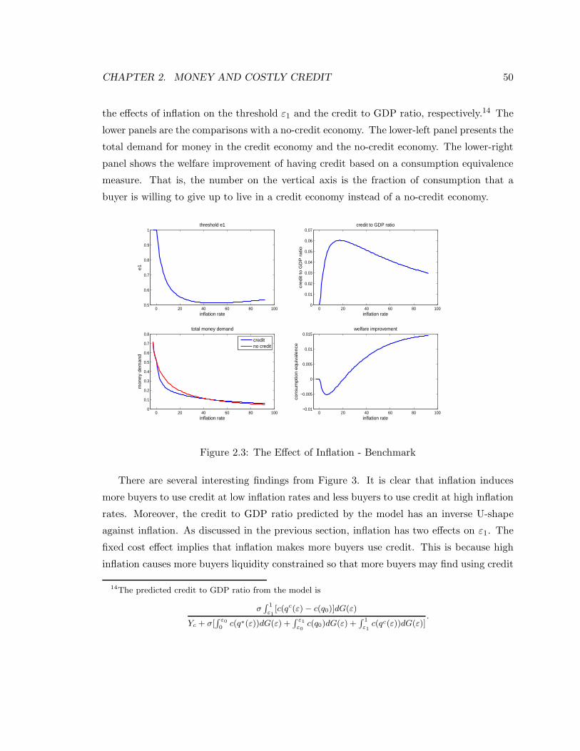
CHAPTER 2. MONEY AND COSTLY CREDIT 50
the effects of inflation on the threshold ε1 and the credit to GDP ratio, respectively.14 The
lower panels are the comparisons with a no-credit economy. The lower-left panel presents the
total demand for money in the credit economy and the no-credit economy. The lower-right
panel shows the welfare improvement of having credit based on a consumption equivalence
measure. That is, the number on the vertical axis is the fraction of consumption that a
buyer is willing to give up to live in a credit economy instead of a no-credit economy.
0 20 40 60 80 1000.5
0.6
0.7
0.8
0.9
1threshold e1
inflation rate
e1
0 20 40 60 80 1000
0.01
0.02
0.03
0.04
0.05
0.06
0.07credit to GDP ratio
inflation rate
cre
dit
to G
DP
ra
tio
0 20 40 60 80 1000
0.1
0.2
0.3
0.4
0.5
0.6
0.7
0.8total money demand
inflation rate
mo
ne
y d
em
an
d
0 20 40 60 80 100−0.01
−0.005
0
0.005
0.01
0.015welfare improvement
inflation rate
con
sum
ptio
n e
qu
iva
len
ce
creditno credit
Figure 2.3: The Effect of Inflation - Benchmark
There are several interesting findings from Figure 3. It is clear that inflation induces
more buyers to use credit at low inflation rates and less buyers to use credit at high inflation
rates. Moreover, the credit to GDP ratio predicted by the model has an inverse U-shape
against inflation. As discussed in the previous section, inflation has two effects on ε1. The
fixed cost effect implies that inflation makes more buyers use credit. This is because high
inflation causes more buyers liquidity constrained so that more buyers may find using credit
14The predicted credit to GDP ratio from the model is
σ∫ 1
ε1
[c(qc(ε) − c(q0)]dG(ε)
Yc + σ[∫ ε0
0c(q∗(ε))dG(ε) +
∫ ε1
ε0
c(q0)dG(ε) +∫ 1
ε1
c(qc(ε))dG(ε)].
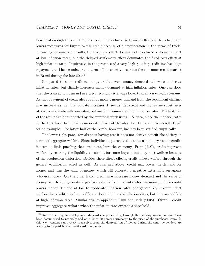
CHAPTER 2. MONEY AND COSTLY CREDIT 51
beneficial enough to cover the fixed cost. The delayed settlement effect on the other hand
lowers incentives for buyers to use credit because of a deterioration in the terms of trade.
According to numerical results, the fixed cost effect dominates the delayed settlement effect
at low inflation rates, but the delayed settlement effect dominates the fixed cost effect at
high inflation rates. Intuitively, in the presence of a very high γ, using credit involves high
repayment and hence unfavorable terms. This exactly describes the consumer credit market
in Brazil during the late 80s.15
Compared to a no-credit economy, credit lowers money demand at low to moderate
inflation rates, but slightly increases money demand at high inflation rates. One can show
that the transaction demand in a credit economy is always lower than in a no-credit economy.
As the repayment of credit also requires money, money demand from the repayment channel
may increase as the inflation rate increases. It seems that credit and money are substitutes
at low to moderate inflation rates, but are complements at high inflation rates. The first half
of the result can be supported by the empirical work using U.S. data, since the inflation rates
in the U.S. have been low to moderate in recent decades. See Duca and Whitesell (1995)
for an example. The latter half of the result, however, has not been verified empirically.
The lower-right panel reveals that having credit does not always benefit the society in
terms of aggregate welfare. Since individuals optimally choose to use money versus credit,
it seems a little puzzling that credit can hurt the economy. From (2.27), credit improves
welfare by relaxing the liquidity constraint for some buyers, but may hurt welfare because
of the production distortion. Besides these direct effects, credit affects welfare through the
general equilibrium effect as well. As analyzed above, credit may lower the demand for
money and thus the value of money, which will generate a negative externality on agents
who use money. On the other hand, credit may increase money demand and the value of
money, which will generate a positive externality on agents who use money. Since credit
lowers money demand at low to moderate inflation rates, the general equilibrium effect
implies that credit may hurt welfare at low to moderate inflation rates, but improve welfare
at high inflation rates. Similar results appear in Chiu and Meh (2008). Overall, credit
improves aggregate welfare when the inflation rate exceeds a threshold.
15Due to the long time delay in credit card charges clearing through the banking system, vendors havebeen documented to normally add on a 20 to 30 percent surcharge to the price of the purchased item. Inthis way, vendors can protect themselves from the depreciation of money during the time the vendors arewaiting to be paid by the credit card companies.
CHAPTER 2. MONEY AND COSTLY CREDIT 52
In terms of the effect of monetary policy, the model predicts that aggregate welfare and
aggregate output are decreasing in the inflation rate. This is not surprising although the
model does introduce a channel through which inflation may potentially increase output
levels at low inflation rates by encouraging more buyers to use credit. However, the effect
from this channel does not appear to be strong.
In Figure 3, the threshold value for credit to improve welfare is around 20% inflation
rate, which is fairly high. The potential problem is that fitting (ρ,B, k) together implicitly
assumes that these parameters do not change over the hundred years. However, it is hard
to believe that the cost of credit transactions stays constant over time. Nevertheless, since
there is no direct data that measures how k evolves over time and the focus of the paper
is not to match any moment in the data, I take a simple approach to evaluate the model‘s
predictions by varying k and fixing (ρ,B). To highlight the effect of changing k, I show in
Figure 4 the credit to GDP ratio and the welfare improvement when k = 0.01, 0.05 and 0.1.
0 20 40 60 80 1000
0.02
0.04
0.06
0.08
0.1
0.12credit to GDP ratio
inflation rate
cred
it to
GD
P ra
tio
0 20 40 60 80 100−0.01
−0.005
0
0.005
0.01
0.015
0.02
0.025
0.03
0.035welfare improvement
inflation rate
cons
umpt
ion
equi
vale
nce
k=0.01k=0.05k=0.1
k=0.01k=0.05k=0.1
Figure 2.4: Comparative Statics - Varying k
According to Figure 4, a lower cost of credit promotes the use of credit. Using the
average inflation rate 7.387 from 1969 − 2000, the predicted credit to GDP ratio is 0.26%
and the predicted real money demand is 0.395 when k = 0.1. For k = 0.01, the predicted
credit to GDP ratio is 10.02% and the predicted real money demand is 0.201. The low cost
credit regime is featured by more credit and less real money demand. It has been noted that
there is a trend decline in real money demand in the recent decade, which has been viewed
CHAPTER 2. MONEY AND COSTLY CREDIT 53
as a shift of the money demand curve.16 Clearly, improvements in the credit transaction
technology contribute to the trend decline in real money demand.
In terms of welfare, more costly credit makes credit less beneficial to the society. One can
see that the threshold for credit to be welfare-improving is higher when k is higher. In the
real world, if sellers receive repayment in the form of money, they may put the money into
their saving accounts to avoid any inflation distortion, which makes credit more beneficial.
This type of argument can be built into the model by allowing a fraction of agents to settle
in market 2 and the rest to settle in market 3. While this is a nice extension, the current
model still serves as a benchmark for analyzing the effect of inflation on credit in a world
in which credit is not entirely free of inflation distortion.
As a robustness check, I choose values of (ρ,B) by varying the sample period and evaluate
the model’s predictions. In these experiments, the value of ρ varies from 0.387 to 0.589,
but the value of B does not change much, which is around 1.4. In terms of the model’s
predictions, the patterns emerging from Figure 3 are very robust.
To study how introducing credit affects the welfare cost of inflation, I compute the
welfare cost of 10% inflation based on the parameters given in Table 1. The measure of
the welfare cost follows the recent literature by using the consumption equivalence measure.
The numbers reported in Table 2 is the fraction of consumption a buyer is willing to give up
to have 0% inflation rather than 10% inflation. As a benchmark, I compute the welfare cost
for a no-credit economy, i.e., k = ∞ and hence ε1 = 1. The welfare cost of 10% inflation is
1.12% in the benchmark economy, which is relatively small because I use take-it-or-leave-it
offer by buyers during bargaining.17
Table 2.2: Welfare Cost of 10% inflationk benchmark 0.01 0.05 0.0739 0.1
Welfare Cost 1.12% 0.22% 0.85% 1.32% 1.40%
I then compute the welfare cost of inflation for different values of k. The introduction
16Considering an economy without credit, I can find the values of (ρ, B) by fitting the money demandcurve. Starting in the 1980s, the predicted money demand diverges from the data. If one is willing to assumea specific functional form of the trend of financial innovation and assume that each year is in a steady state,then fitting the money demand data can generate the values of (ρ, B) and the trend of financial innovation.By doing such an exercise, I found that the predicted money demand in recent years is much closer to themoney demand data. A similar exercise is in Faig and Jerez (2006).
17In Lagos and Wright (2005), the welfare cost of 10% inflation is 1.4% when buyers have all the bargainingpower. The current result does not deviate from their estimate.
CHAPTER 2. MONEY AND COSTLY CREDIT 54
of credit can raise the welfare cost when credit is costly enough. For low values of k, the
cost for buyers to substitute credit for money is relatively low. Therefore, inflation does not
generate a large welfare loss. On the contrary, if the cost for buyers to switch from money
to credit is high, inflation can result in a higher welfare loss compared to the benchmark
economy. Note that if k is too big, no buyer uses credit and the economy is essentially
the benchmark economy. Dotsey and Ireland (1996) and Lacker and Shreft (1996) both
emphasize that credit costs are quantitatively important as a component of the welfare cost
of inflation. The results in Table 2 further confirm their results.
2.5 Monetary Equilibrium without Enforcement
So far I have assumed that financial intermediaries can enforce the repayment of credit,
which implies that buyers are not credit constrained. In this section, I relax the assumption
of perfect enforcement. Financial intermediaries can identify agents and keep records of
goods market transactions, but they cannot enforce the repayment of credit. As in Berentsen
et al. (2007) and Sanches and Williamson (2008), the punishment for default is permanent
exclusion from the financial system. That is, if a buyer defaults, the buyer will never be able
to use credit in any future period. Given the punishment, the amount of credit extended
to a buyer is consistent with the buyer’s incentive to repay. In an environment without
enforcement, the government (or the monetary authority) cannot enforce buyers to pay
taxes either. It implies that γ ≥ 1.
With this modification, buyers and sellers face the same choice problems as before in
market 2 and 3. Only in market 1, the buyer’s take-it-or-leave-it offer should be reformu-
lated.
maxq,d,a
[εu(q) − φd − φa]
s.t. c(q) = φd + βφa, d ≤ m and a ≤ a.
Here a is the credit limit faced by the buyer. An individual buyer takes a as given. In
equilibrium, a will be endogenously determined. The Lagrangian is
L = maxq,d,a,λ1,λ2,λ3
[εu(q) − φd − φa] + λ1[φd + βφa − c(q)] + λ2(m − d) + λ3(a − a).
CHAPTER 2. MONEY AND COSTLY CREDIT 55
If the credit constraint is not binding, i.e., λ3 = 0, then d = m and (q, a) are given by
εu′(q) =γ
βc′(q),
βφa = c(q) − φd.
If the credit constraint is binding, i.e., λ3 > 0, I have d = m, a = a and q solving
c(q) = φd + βφa.
Introducing the credit limit may cause some buyers to be credit constrained. If such buyers
exist, there are potentially four groups of buyers.
Lemma 2.9 For any given inflation rate γ, there exist three thresholds of ε, ε0, ε1 and ε2
such that
0 ≤ ε ≤ ε0, the buyer spends d < m, a = 0, and consumes q∗ where εu′(q∗) = c′(q∗),
ε0 ≤ ε ≤ ε1, the buyer spends d = m, a = 0 and consumes q where c(q) = φm,
ε1 ≤ ε ≤ ε2, the buyer spends d = m, a < a and consumes qc where εu′(qc) = γβc′(qc),
ε2 ≤ ε ≤ 1, the buyer spends d = m, a = a and consumes q where c(q) = φm + βφa.
The expected marginal value of money in market 3 is
β
∫
∂V1(m, 0; ε)
∂mG(ε) = βφ
∫ ε0
0dG(ε) +
∫ ε1
ε0
[σεu′(q0)
c′(q0)+ (1 − σ)]dG(ε)
+
∫ ε2
ε1
[σγ
β+ (1 − σ)]dG(ε) +
∫ 1
ε2
[σεγ
ε2β+ (1 − σ)]dG(ε)
,
where q0 is defined in (2.22). Combining with (2.8), the optimal q0 is implicitly given by
ε0 +1
2
u′(q0)
c′(q0)(ε2
1 − ε20) +
γ
β(ε2 − ε1) +
1
2
γ
β(
1
ε2− ε2) = 1 +
γ − β
βσ. (2.28)
Define q2 such thatε2u
′(q2)
c′(q2)=
γ
β, (2.29)
and q2 satisfies
c(q2) = c(q0) + βφa. (2.30)
Now suppose that ε2 < 1. Consider a buyer with ε carrying debt a into market 2. The
buyer must have spent all of his money. If he repays the debt, the buyer should work to
CHAPTER 2. MONEY AND COSTLY CREDIT 56
accumulate the money for repayment. His value function is V b2 (0, a). If the buyer defaults,
he does not need to work as much in market 2. Denote the payoff from default by V bD2 (0, a)
where
V bD2 (0, a) = v(x∗) − x∗ + max
zD
−φzD + V bD3 (zD, 0)
.
The superscript D represents variables associated with default. The real credit limit is the
value of βφa that solves V b2 (0, a) = V bD
2 (0, a). After some algebra, the real credit limit is
βφa =β2σ
γ(1 − β)
∫ ε0
0[εu(q∗(ε)) − c(q∗(ε))]dG(ε) +
∫ ε1
ε0
[εu(q0) − c(q0)]dG(ε)(2.31)
+
∫ ε2
ε1
[εu(qc(ε)) − k −γ
βc(qc(ε)) + (
γ
β− 1)c(q0)]dG(ε)
+
∫ 1
ε2
[εu(q2) − k −γ
βc(q2) + (
γ
β− 1)c(q0)]dG(ε)
−
∫ εD0
0[εu(q∗(ε) − c(q∗(ε))]dG(ε) −
∫ 1
εD0
[εu(qD0 ) − c(qD
0 )]dG(ε)
+(γ − β)β
γ(1 − β)[c(qD
0 ) − c(q0)].
When the repayment of credit cannot be enforced, a monetary equilibrium with con-
strained credit is defined by a list of (ε0, ε1, ε2, q0, q1, q2, βφa) characterized by (2.22), (2.23),
(2.25), (2.28), (2.29), (2.30) and (2.31). It is possible that (ε1, ε2) hit the boundary 1 in
equilibrium. In particular, there are two special cases: [1] ε2 = 1 and [2] ε1 = ε2 = 1. In
case [1], the equilibrium corresponds to the monetary equilibrium with credit in Section 3.
In case [2], the equilibrium corresponds to the monetary equilibrium without credit. Notice
that in these two cases, the endogenous credit limit still exists, but it is not binding.
It becomes very complicated to derive any analytical results. Hence, I use a numerical
example to show how endogenizing credit limit affects equilibrium and welfare. Based on the
numerical exercise in Section 4, I again set ρ = 0.4732 and B = 1.4436. As for k, I choose
k = 0.03. The left panel in Figure 5 shows the endogenous credit limit and the maximum
amount of borrowing for various inflation rates. The main finding is that buyers are credit
constrained only at very low inflation rates, which is consistent with Berentsen et al. (2007).
High inflation rates help to relax the credit constraint because punishment becomes more
severe. Since inflation also lowers the surplus from credit trades in this model, the overall
effect of inflation on credit limit is that inflation first relaxes and then tightens the credit
limit. At high inflation rates, because buyers borrow less, the credit constraint does not
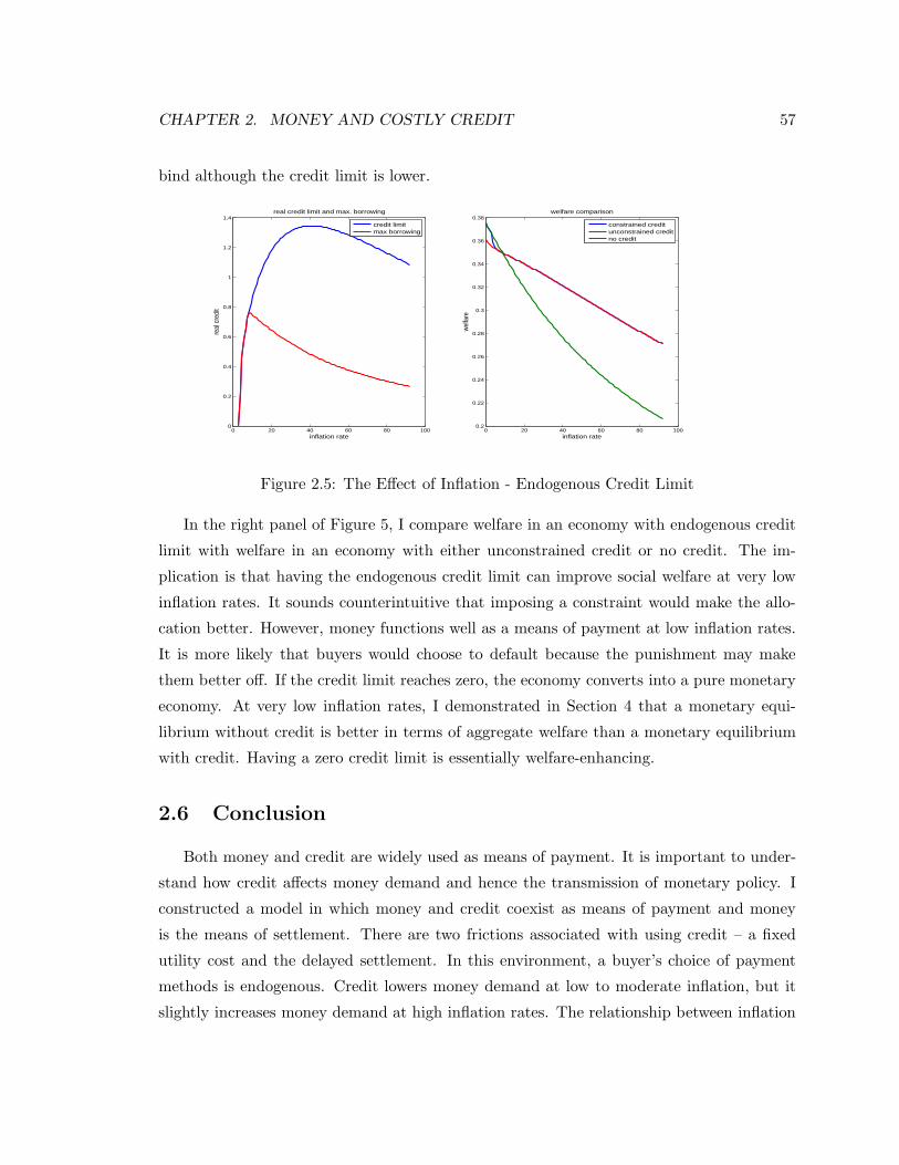
CHAPTER 2. MONEY AND COSTLY CREDIT 57
bind although the credit limit is lower.
0 20 40 60 80 1000
0.2
0.4
0.6
0.8
1
1.2
1.4real credit limit and max. borrowing
inflation rate
real
cre
dit
0 20 40 60 80 1000.2
0.22
0.24
0.26
0.28
0.3
0.32
0.34
0.36
0.38
inflation rate
wel
fare
welfare comparison
credit limitmax borrowing
constrained creditunconstrained creditno credit
Figure 2.5: The Effect of Inflation - Endogenous Credit Limit
In the right panel of Figure 5, I compare welfare in an economy with endogenous credit
limit with welfare in an economy with either unconstrained credit or no credit. The im-
plication is that having the endogenous credit limit can improve social welfare at very low
inflation rates. It sounds counterintuitive that imposing a constraint would make the allo-
cation better. However, money functions well as a means of payment at low inflation rates.
It is more likely that buyers would choose to default because the punishment may make
them better off. If the credit limit reaches zero, the economy converts into a pure monetary
economy. At very low inflation rates, I demonstrated in Section 4 that a monetary equi-
librium without credit is better in terms of aggregate welfare than a monetary equilibrium
with credit. Having a zero credit limit is essentially welfare-enhancing.
2.6 Conclusion
Both money and credit are widely used as means of payment. It is important to under-
stand how credit affects money demand and hence the transmission of monetary policy. I
constructed a model in which money and credit coexist as means of payment and money
is the means of settlement. There are two frictions associated with using credit – a fixed
utility cost and the delayed settlement. In this environment, a buyer’s choice of payment
methods is endogenous. Credit lowers money demand at low to moderate inflation, but it
slightly increases money demand at high inflation rates. The relationship between inflation
CHAPTER 2. MONEY AND COSTLY CREDIT 58
and the credit to GDP ratio exhibits an inverse U-shape which is broadly consistent exist-
ing evidence. Costly credit does not always improve social welfare. Depending on the fixed
utility cost of credit, allowing credit as a means of payment may raise the welfare cost of
inflation.
In a modified environment where enforcement is imperfect, the endogenous credit limit
tends to increase at low inflation rates, but decrease at high inflation rates. However, credit
constraints only bind at very low inflation rates. Interestingly, imperfect enforcement may
improve social welfare because it avoids socially inefficient borrowing.
One testable implication from the model is that the relationship between inflation and
the credit to GDP ratio has an inverse U-shape. There exist many studies testing the long
run effect of inflation on credit. Most of them use the total private credit to GDP ratio as
the measure of credit. To complement this paper, it would be ideal to use the consumer
credit to GDP ratio and test its long run relationship with inflation. As I only obtain the
data on consumer credit in Canada and the U.S., I will pursue this empirical study with
more cross-country data in my future work.18
2.7 Appendix
2.7.1 Use of Credit Card Data
Table 3 describes the U.S. households’ credit card spending volume and credit card debt
outstanding in 2000 and 2005. The numbers reported for 2010 are projections. Data are
from U.S. Statistical Abstract.
2.7.2 Proof of Lemma 2.1
Proof. As discussed in the paper, if a buyer uses credit, he must spend all his money. Define
q as the solution to εu′(q) = c′(q). One can show that φm < c(q) as long as γ > β. It implies
that there exists a threshold ε0 such that ε0u′(q0) = c′(q0) where q0 is from c(q0) = φz. For
18I tested the long run relationship between inflation and the private credit to GDP ratio following Bullardand Keating (1995). The results moderately support the inverse U-shape prediction. In addition, I usedCanada and the U.S. consumer credit data to perform the same test. For these two low inflation countries, apermanent increase in inflation increases the consumer credit to GDP ratio, which is consistent with the lefthalf of the inverse U-shape. However, due to data availability, I do not have any consumer credit data forhigh inflation countries. Therefore, it is hard to verify the right half of the U-shape at this stage. A detaileddescription of the estimation is available upon request.
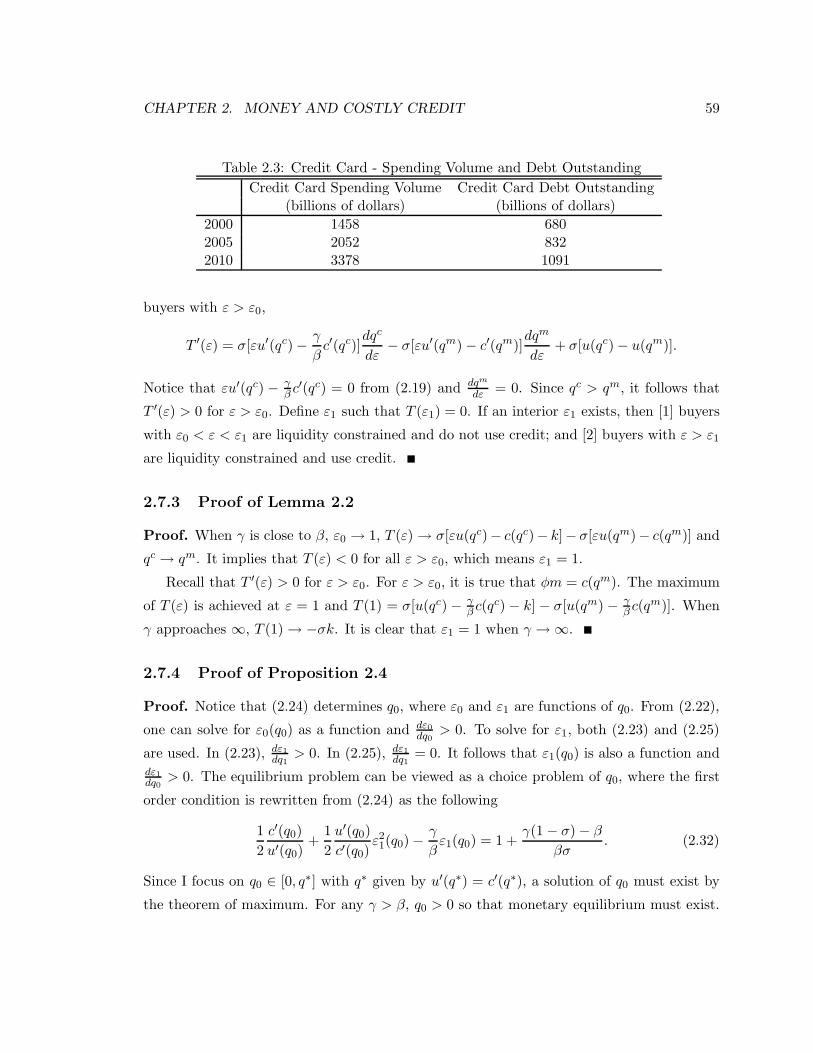
CHAPTER 2. MONEY AND COSTLY CREDIT 59
Table 2.3: Credit Card - Spending Volume and Debt Outstanding
Credit Card Spending Volume Credit Card Debt Outstanding(billions of dollars) (billions of dollars)
2000 1458 6802005 2052 8322010 3378 1091
buyers with ε > ε0,
T ′(ε) = σ[εu′(qc) −γ
βc′(qc)]
dqc
dε− σ[εu′(qm) − c′(qm)]
dqm
dε+ σ[u(qc) − u(qm)].
Notice that εu′(qc) − γβc′(qc) = 0 from (2.19) and dqm
dε= 0. Since qc > qm, it follows that
T ′(ε) > 0 for ε > ε0. Define ε1 such that T (ε1) = 0. If an interior ε1 exists, then [1] buyers
with ε0 < ε < ε1 are liquidity constrained and do not use credit; and [2] buyers with ε > ε1
are liquidity constrained and use credit.
2.7.3 Proof of Lemma 2.2
Proof. When γ is close to β, ε0 → 1, T (ε) → σ[εu(qc)− c(qc)− k]− σ[εu(qm)− c(qm)] and
qc → qm. It implies that T (ε) < 0 for all ε > ε0, which means ε1 = 1.
Recall that T ′(ε) > 0 for ε > ε0. For ε > ε0, it is true that φm = c(qm). The maximum
of T (ε) is achieved at ε = 1 and T (1) = σ[u(qc) − γβc(qc) − k] − σ[u(qm) − γ
βc(qm)]. When
γ approaches ∞, T (1) → −σk. It is clear that ε1 = 1 when γ → ∞.
2.7.4 Proof of Proposition 2.4
Proof. Notice that (2.24) determines q0, where ε0 and ε1 are functions of q0. From (2.22),
one can solve for ε0(q0) as a function and dε0dq0
> 0. To solve for ε1, both (2.23) and (2.25)
are used. In (2.23), dε1dq1
> 0. In (2.25), dε1dq1
= 0. It follows that ε1(q0) is also a function anddε1dq0
> 0. The equilibrium problem can be viewed as a choice problem of q0, where the first
order condition is rewritten from (2.24) as the following
1
2
c′(q0)
u′(q0)+
1
2
u′(q0)
c′(q0)ε21(q0) −
γ
βε1(q0) = 1 +
γ(1 − σ) − β
βσ. (2.32)
Since I focus on q0 ∈ [0, q∗] with q∗ given by u′(q∗) = c′(q∗), a solution of q0 must exist by
the theorem of maximum. For any γ > β, q0 > 0 so that monetary equilibrium must exist.
CHAPTER 2. MONEY AND COSTLY CREDIT 60
Similar to the proof in Wright (2008), one can show that equilibrium q0 is unique for generic
values of σ. However, it is not obvious that equilibrium q0 is unique for generic values of γ
in this model.
2.7.5 Proof of Proposition 2.5
Proof. Total differentiate (2.24), (2.22), (2.23) and (2.25) with respect to k:
c′(q0)u′′(q0) − u′(q0)c
′′(q0)
2[c′(q0)]2(ε2
1 − ε20)
dq0
dk+ [ε1
u′(q0)
c′(q0)−
γ
β]dε1
dk= 0,
c′(q0)u′′(q0) − u′(q0)c
′′(q0)
[c′(q0)]2dq0
dk+
1
ε20
dε0
dk= 0,
c′(q1)u′′(q1) − u′(q1)c
′′(q1)
[c′(q1)]2dq1
dk+
γ
βε21
dε1
dk= 0,
[u(q1) − u(q0)]dε1
dk− 1 − [ε1u
′(q0) −γ
βc′(q0)]
dq0
dk= 0.
From (2.25), one can show that q1 > q0. Together with (2.22) and (2.23), ε1u′(q0)c′(q0) − γ
β> 0.
It follows that dε0dk
, dq0
dk, dε0
dkand dε1
dkare equal in sign. Moreover,
c′(q0)u
′′(q0) − u′(q0)c′′(q0)
2[c′(q0)]2(ε2
1−ε20)+
[ε1u′(q0)c′(q0) −
γβ][ε1u
′(q0) −γβc′(q0)]
[u(q1) − u(q0)]dq0
dk=
1
u(q0) − u(q1).
(2.33)
Define
f(q0; γ) = ε0(q0) +1
2
u′(q0)
c′(q0)[ε2
1(q0) − ε20(q0)] +
γ
β[1 − ε1(q0)] − 1 −
γ − β
βσ,
where ε0(q0) is from (2.22) and ε1(q0) is from (2.23) and (2.25). As the equilibrium q0 must
be local maximum, it must be true that f ′(q0; γ) < 0, so
c′(q0)u′′(q0) − u′(q0)c
′′(q0)
2[c′(q0)]2(ε2
1 − ε20) +
[ε1u′(q0)c′(q0)
− γβ][ε1u
′(q0) −γβc′(q0)]
[u(q1) − u(q0)]< 0. (2.34)
From (2.33), I have dq0
dk> 0 and hence, dε0
dk> 0, dε1
dk> 0 and dq1
dk> 0.
CHAPTER 2. MONEY AND COSTLY CREDIT 61
2.7.6 Proof of Proposition 2.7
Proof. The proof is similar to the proof of Proposition 2. Total differentiate (2.24), (2.22),
(2.23) and (2.25) with respect to σ:
c′(q0)u′′(q0) − u′(q0)c
′′(q0)
2[c′(q0)]2(ε2
1 − ε20)
dq0
dσ+ [ε1
u′(q0)
c′(q0)−
γ
β]dε1
dσ= −
γ − β
βσ2,
c′(q0)u′′(q0) − u′(q0)c
′′(q0)
[c′(q0)]2dq0
dσ+
1
ε20
dε0
dσ= 0,
c′(q1)u′′(q1) − u′(q1)c
′′(q1)
[c′(q1)]2dq1
dσ+
γ
βε21
dε1
dσ= 0,
[u(q1) − u(q0)]dε1
dσ− [ε1u
′(q0) −γ
βc′(q0)]
dq0
dσ= 0.
It is clear that dε0dσ
, dq0
dσ, dε1
dσand dε1
dσhave the same sign. Using (2.34), dq0
dσ> 0. Moreover,
dε0dk
> 0, dε1dk
> 0 and dq1
dk> 0.
2.7.7 Proof of Proposition 2.8
Proof. The proof is similar to the proofs of Proposition 2 and Proposition 3. Total differ-
entiate (2.24), (2.22), (2.23) and (2.25) with respect to γ:
c′(q0)u′′(q0) − u′(q0)c
′′(q0)
2[c′(q0)]2(ε2
1 − ε20)
dq0
dγ+ [ε1
u′(q0)
c′(q0)−
γ
β]dε1
dγ=
1
βσ−
1 − ε1
β,
c′(q0)u′′(q0) − u′(q0)c
′′(q0)
[c′(q0)]2dq0
dγ+
1
ε20
dε0
dγ= 0,
c′(q1)u′′(q1) − u′(q1)c
′′(q1)
[c′(q1)]2dq1
dγ+
γ
βε21
dε1
dγ=
1
βε1,
[u(q1) − u(q0)]dε1
dγ− [ε1u
′(q0) −γ
βc′(q0)]
dq0
dγ=
1
β[c(q1) − c(q0)].
Using (2.34), the sign of dq0
dγis the same as the sign of h(ε0, ε1, q0, q1), where
h(ε0, ε1, q0, q1) =1 − ε1
β+ (
ε1
ε0−
γ
β)
c(q1) − c(q0)
β[u(q1) − u(q0)]−
1
βσ. (2.35)
From (2.25),c(q1) − c(q0)
β[u(q1) − u(q0)]<
ε1
γ.
It follows that h(ε0, ε1, q0, q1) < 1β(1 − 1
σ− 2ε1 + ε1
ε1βε0γ
). Derivingε21
ε0from (2.24),
1
β(1 −
1
σ− 2ε1 + ε1
ε1β
ε0γ) =
1
γ[(2 −
γ
β)(1 −
1
σ) − ε0].
CHAPTER 2. MONEY AND COSTLY CREDIT 62
One can show that h(ε0, ε1, q0, q1) < 0 when either σ = 1 or γβ≤ 2. As a result, dq0
dγ< 0 and
dε0dγ
< 0 when σ = 1 or γβ≤ 2.
2.7.8 Proof of Lemma 2.9
Proof. The proof is similar to the proof of Lemma 1. From (2.19), q is increasing in ε for
any given γ. An individual buyer takes the credit limit a as given. If ε is large enough,
the buyer may face a binding credit limit and the maximum amount q that the buyer can
consume is given by c(q) = φm + βφa.
2.8 References
Aiyagari, Rao, Anton Braun and Zvi Eckstein (1998), ”Transaction Services, Inflation, and
Welfare”, Journal of Political Economy, Vol. 106 (6), pp. 1274-1301.
Azariadis, Costas and Bruce Smith (1996), ”Private Information, Money, and Growth:
Indeterminacy, Fluctuations, and the Mundell-Tobin Effect”, Journal of Economics
Growth, 1, pp. 309-332.
Berentsen, Aleksander, Gabriele Camera and Christopher Waller (2007), ”Money, Credit
and Banking”, Journal of Economic Theory, Vol. 135 (1), pp. 171-195.
Boyd, John and Bruce Champ (2003), ”Inflation and Financial Market Performance: What
Have We Learned in the Last Ten Years?”, Federal Reserve Bank of Cleveland, working
paper, 03-17.
Boyd, John, Ross Levine and Bruce Smith (2001), ”The Impact of Inflation on Financial
Sector Performance”, Journal of Monetary Economics, 47, pp. 221-248.
Bullard, James and Keating (1995), ”The Long-run Relationship between Inflation and
Output in Postwar Economies”, Journal of Monetary Economics, 36, pp. 477-496.
Cavalcanti, Ricardo and Neil Wallace (1999), ”Inside and Outside Money as Alternative
Media of Exchange”, Journal of Money, Credit and Banking, Vol 31 (3), pp. 443-457.
Chiu, Jonathan and Cesaire Meh (2008), ”Banking, Liquidity and Inflation”, Bank of
Canada, working paper.
CHAPTER 2. MONEY AND COSTLY CREDIT 63
Craig, Ben and Guillaume Rocheteau (2007), ”Inflation and Welfare: A Search Approach”,
Journal of Money, Credit and Banking, forthcoming.
Dotsey, Michael and Peter Ireland (1996), ”The Welfare Cost of Inflation in General Equi-
librium”, Journal of Monetary Economics, Vol. 37 (1), pp. 29-47.
Duca, John V. and William C. Whitesell (1995), ”Credit Cards and Money Demand: A
Cross-sectional Study”, Journal of Money, Credit and Banking, Vol. 27, No. 2, pp.
604-623.
English, William, (1999), ”Inflation and Financial Sector Size”, Journal of Monetary Eco-
nomics, 44 (3), pp. 379-400.
Faig, Miquel and Belen Jerez (2006), ”Precautionary Balance and the Velocity of Circulation
of Money”, Journal of Money, Credit and Banking, 39 (4), pp. 843-873.
Ferraris, Leo (2006), ”On the Complementarity of Money and Credit”, Universidad Carlos
III de Madrid, working paper.
Freeman, Scott and Gregory Huffman (1991), ”Inside Money, Output, and Causality”, In-
ternational Economic Review, 32, pp. 645-667.
Kahn, Mohsin, Abdelhak Senhadji and Bruce Smith (2006), ”Inflation and Financial Depth”,
Macroeconomic Dynamics, 10, pp. 165-182.
Klee, Elizabeth (2008), ”How People Pay: Evidence from Grocery Store Data”, Journal of
Monetary Economics, 55, pp. 526-541.
Kocherlakota, Narayana and Neil Wallace (1999), ”Incomplete Record-Keeping and Optimal
Payment Arrangements”, Journal of Economic Theory, Vol. 81, Issue 2, pp. 272-289.
Lacker, J. and Stacey Shreft (1996), ”Money and Credit as Means of Payment”, Journal of
Monetary Economics, 38, pp. 3-23.
Lagos, Ricardo and Randall Wright (2005), ”A Unified Framework for Monetary Theory
and Policy Analysis”, Journal of Political Economy, Vol. 113 (3), pp. 463-484.
Lester, Ben, Andrew Postlewaite and Randall Wright (2008), ”Information, Liquidity and
Asset Prices”, PIER working paper, 08-039.
CHAPTER 2. MONEY AND COSTLY CREDIT 64
Lucas, Robert E. (2000), ”Inflation and Welfare”, Econometrica, Vol. 68, No. 2, pp. 247-
274.
Mills, David (2007), ”A Model in which Outside and Inside Money are Essential”, Macroe-
conomics Dynamics, 11, pp. 347-366.
Sanches, Daniel and Stephen Williamson (2008), ”Money and Credit with Limited Commit-
ment and Theft”, Washington University in St. Louis, working paper.
Stockman, Alan (1981), ”Anticipated Inflation and the Capital Stock in a Cash-in-Advance
economy”, Journal of Monetary Economics, 8, pp. 387-393.
Sun, Hongfei (2007), ”Banking, Inside Money and Outside Money”, QED working paper,
No. 1146.
Telyukova, Irina and Randall Wright (2008), ”A Model of Money and Credit, with Ap-
plication to the Credit Card Debt Puzzle”, Review of Economic Studies, 75 (2), pp.
629-647.
Wright, Randall (2008), ”A Uniqueness Proof for Monetary Steady State”, University of
Pennsylvania, working paper.
Chapter 3
One or Two Monies?1
3.1 Introduction
Micro-founded monetary theory explains how an intrinsically useless object can be valued
in exchange. Recent advances in the literature seem to have reached a consensus that the
role of money is to make up for the missing memory or the record-keeping technology, i.e.,
see Kocherlakota (1998a, b). A natural question to follow is whether money constitutes a
perfect substitute for the record-keeping technology. Most micro-founded monetary models
feature one single money and there is no welfare-enhancing role for a second money. In this
paper, we show that when money is divisible, concealable and in variable supply, a single
money might or might not be sufficient to replace the record-keeping technology. We then
show that in the latter case, introducing a second money improves welfare, and that two
monies act as a perfect substitute for the record-keeping technology.
We construct a heterogeneous agent model in a quasilinear environment as introduced
by Lagos and Wright (2005). There are two types of agents and two locations indexed by
a and b. In every period, a location/preference shock randomly assigns agents to one of the
two locations and determines their marginal utilities from consumption. Type a (b) agents
have high marginal utilities at location a (b) and low marginal utilities at location b (a).
1This is a joint paper with Janet Hua Jiang. We would like to thank David Andolfatto, Robert Jones,Alexander Karaivanov, Fernando Martin, Ed Nosal, Chris Waller, Randy Wright, and participants at thebrown bag seminar at Simon Fraser University, the 2007 Cleveland Federal Reserve Conference on Money,Banking, Payments, and Finance, the 2008 Midwest Macro Meetings, the 2008 Canadian Economic Asso-ciation Meetings and the 2008 Econometrica North America Summer Meetings for helpful suggestions andcomments.
65
CHAPTER 3. ONE OR TWO MONIES? 66
Since agents at the same location are endowed with the same amount of goods, the first-best
allocation requires that agents with low marginal utilities transfer some of their endowment
to agents with high marginal utilities.
There are two frictions in the economy: limited commitment and private information
about types. In the presence of the these frictions, an implementable allocation must be
incentive compatible to ensure participation and truthful revelation of types. Throughout
the paper, we adopt a mechanism design approach and solve the conditions under which
the first-best allocation satisfies the relevant incentive constraints.
We first analyze mechanisms with a perfect record-keeping technology. The mechanism
can directly record nonparticipation and impose perpetual autarky as the punishment for
nonparticipation.2 With regard to private information, the mechanism asks agents to report
their types, records the information and uses it later on to infer agents’ marginal utilities.
Due to the symmetry structure of the preferences, agents have the incentive to truthfully
report their types ex ante (we call this ‘early-sorting’ because the incentive is aligned before
the realization of the location shock) at the first-best allocation. The first-best allocation
can be achieved as long as the participation constraint is satisfied, or agents are patient
enough.
Next, we assume that the record-keeping technology is not available, but the society has
access to one fiat money. By rewarding participants with more money and requiring an ever
increasing amount of money for future participation, one-money mechanisms can deal with
limited commitment as effectively as mechanisms with the record-keeping technology. How-
ever, one-money mechanisms are not as powerful in dealing with private information. With
a single concealable money, encoding and passing information on ex ante type reporting
becomes problematic. Different reports can only be encoded into different money balances,
which however, can be hidden to prevent credible information communication. In this case,
the only effective way to deal with private information is to induce agents to reveal their
types/marginal utilities after the period location shock (we call this ‘late-sorting’).
Due to quasilinearity, the late-sorting mechanism involves no ex ante welfare cost; it,
however, imposes an extra constraint on the patience parameter. As a result, the restriction
on the patience parameter to implement the first-best allocation is more stringent than with
the record-keeping technology. There exists a positive measure of the patience parameter
2We assume that the most severe societal penalty is ostracism.
CHAPTER 3. ONE OR TWO MONIES? 67
such that the first-best allocation can be achieved with the record-keeping technology, but
not with one money. Hence, one money is not a perfect substitute for the record-keeping
technology in the quasilinear environment that we consider.
We then investigate mechanisms when a second money is introduced. We find that hav-
ing two monies allows the mechanism to use monetary portfolios and total money balances
to record ex ante reporting about types. Moreover, the information can be credibly passed
into the future. It follows that two monies act as a perfect substitute for the record-keeping
technology. We also extend the above results to an environment with more than two types of
agents. We argue in general that two monies are a perfect substitute for the record-keeping
technology so that there is no need for a third money.
Our work is most closely related to Kocherlakota and Krueger (1999), and Kocherlakota
(2002) which also study the essentiality of multiple monies.3
Kocherlakota and Krueger (1999) share with us a common feature that a second money
improves welfare in that a second money serves as a signalling device to deal with private
information. Their model, however, builds on Trejos and Wright (1995) with indivisible
money. The result that there is no need for a third money cannot be extended to multiple-
type-agent models. Moreover, the quasilinear preferences in our model introduce an addi-
tional way (the late-sorting mechanism) to align incentives. It follows that a second money
is inessential if agents are patient enough (because late-sorting is powerful enough to deal
with both private information and limited commitment).
Kocherlakota (2002) correctly points out that when money is concealable, it is necessary
to establish a monotonic relationship between ‘proper’ behavior and money balances. In
Kocherlakota (2002), limited commitment makes it impossible to establish such a relation-
ship and renders the need for a second money. This conclusion, however, hinges critically
on the assumption of a fixed money supply. When money supply is fixed, the only way to
record whether an agent behaves properly is to transfer some money to him from somebody
else (who might also behave properly). Agents’ money holdings will differ in general. The
first-best allocation, however, requires that future allocation should not discriminate those
with less money balances. The mechanism that we propose circumvents the problem by
3There is another strand of literature investigating whether multiple currencies can coexist or circulate atthe same time. Examples are Trejos and Wright (2001), Camera and Winkler (2003), Camera et al. (2004),and Craig and Waller (2004). Our paper’s goal is to study the welfare enhancing role of multiple currencies,or whether multiple currencies are essential.
CHAPTER 3. ONE OR TWO MONIES? 68
increasing money supply to reward all properly behaved participants. Limited commitment
thus does not justify a role for a second money if money supply is allowed to change.
The rest of the paper proceeds as follows. Section 2 lays out the physical environment
and characterizes the first-best allocation. Section 3 introduces private information and
limited commitment. We solve for the condition to achieve the first-best allocation when the
society has access to a record-keeping technology. Section 4 studies the optimal monetary
mechanisms when the record-keeping technology is absent, and establishes the condition
under which a second money is essential. Section 5 extends the results to a multi-type-
agent model. Section 6 argues in general that two monies constitute a perfect substitute
for the record-keeping technology. We conclude and suggest directions for future research
in section 7.
3.2 The Physical Environment
The framework that we adopt is the quasi-linear environment suggested by Lagos and
Wright (2005) without the search friction. Time is discrete and runs from 0 to ∞. Each
period consists of two stages: day and night. There are two locations a and b. Inter-location
interaction is allowed during the day but prohibited at night. There are three non-storable
goods, one day good and two location-specific night goods indexed by 1 and 2. Good 1 is
local to location a and good 2 is local to location b. There are two types of agents – each is
of measure 1.
During the day, all agents can produce or consume the day good. They have the same
linear preference over the good. Let z be the amount of production (consumption if z is
negative). The disutility of production (utility of consumption if z is negative) is −z.
At night, agents consume one of the two night goods. The two types of agents are
distinguished by their preferences over the two night goods. Type a value good 1 more
than good 2, and type b value good 2 more than good 1. It might be helpful to think of
type a as local consumers of good 1 and foreign consumers of good 2; similarly, think of
type b as local consumers of good 2 and foreign consumers of good 1. The utility of a local
consumer is δu(c) and the utility of a foreigner is u(c), where δ > 1, u(0) = 0, u′′ < 0 < u′
and u′(0) = +∞. Which night good an agent consumes is determined by a preference shock
realized upon entering the night stage. With probability 1/2, an agent becomes a local
consumer and has a high valuation of the night good. With probability 1/2, the agent
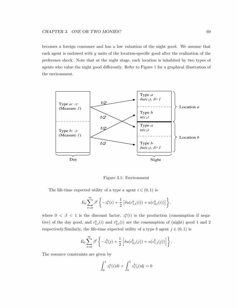
CHAPTER 3. ONE OR TWO MONIES? 69
becomes a foreign consumer and has a low valuation of the night good. We assume that
each agent is endowed with y units of the location-specific good after the realization of the
preference shock. Note that at the night stage, each location is inhabited by two types of
agents who value the night good differently. Refer to Figure 1 for a graphical illustration of
the environment.
Type a
u(c1), >1
Type b
u(c1)
Night
Type a: -z
(Measure 1)
Type b: -z
(Measure 1)
Day
Location a
Type a
u(c2)
Type b
u(c2), >1
Location b
Figure 3.1: Environment
The life-time expected utility of a type a agent i ∈ (0, 1) is
E0
∞∑
t=0
βt
−zat (i) +
1
2
[
δu(ca1,t(i)) + u(ca
2,t(i))]
.
where 0 < β < 1 is the discount factor, zat (i) is the production (consumption if nega-
tive) of the day good, and ca1,t(i) and ca
2,t(i) are the consumption of (night) good 1 and 2
respectively.Similarly, the life-time expected utility of a type b agent j ∈ (0, 1) is
E0
∞∑
t=0
βt
−zbt (j) +
1
2
[
δu(cb2,t(j)) + u(cb
1,t(j))]
.
The resource constraints are given by
∫ 1
0zat (i)di +
∫ 1
0zbt (j)dj = 0
CHAPTER 3. ONE OR TWO MONIES? 70
at the day stage, and∫ 1
0ca1,t(i)I
at (i)di +
∫ 1
0cb1,t(j)I
at (j)dj = y at location a,
∫ 1
0ca2,t(i)I
bt (i)di +
∫ 1
0cb2,t(j)I
bt (j)dj = y at location b,
at the night stage for all t ≥ 0. Ikt (•) is an indicator function and is equal to 1 if the agent
is at location k ∈ a, b at date t.
We will focus on symmetric stationary allocations where for all i and j ∈ (0, 1) and
k ∈ a, b,
• ca1,t(i) = cb
2,t(j) = ch, ca2,t(j) = cb
1,t(i) = cℓ with ch + cℓ = 2y for t ≥ 0;
• za0 (i) = zb
0(j) = 0;
• zkt (·) =
zh, if the agent consumed ch at the night stage of time t − 1;
zℓ, if the agent consumed cℓ at the night stage of time t − 1;
with zh + zℓ = 0 for t ≥ 1.
The social planner’s problem is to choose (ch, cℓ, zh, zℓ) to maximize the ex ante utility
W (ch, cℓ, y) =1
2
1
1 − β[δu(ch) + u(cℓ)] (3.1)
s.t. ch + cℓ = 2y.
The solution is characterized by
δu′(c∗h) = u′(c∗ℓ ),
c∗h + c∗ℓ = 2y,
W ∗ =1
2
1
1 − β[δu(c∗h) + u(c∗ℓ )] .
Note that since δ > 1, c∗h > y > c∗ℓ . The planner can instruct the night stage low-valuation
agents to ‘lend’ τ∗ ≡ y − c∗ℓ units of his endowment to high-valuation agents. For the day
stage allocation, note that since zt enters linearly in preferences, any zat (i) and zb
t (j) that
satisfy E0zat (i) = E0z
bt (j) = 0 would satisfy the day stage resource constraint and entail no
ex ante welfare loss. In the current context, one such allocation is zat (i) = zb
t (j) = 0 for all
i and j and t ≥ 0.
The first-best allocation can be achieved if agents’ types are public information, and
agents are able to commit to sticking with the allocation.
CHAPTER 3. ONE OR TWO MONIES? 71
3.3 Limited Commitment and Private Information
Assume that agents cannot commit, and agents’ types and thus their valuations of the
night goods are private information. In this case, a record-keeping technology becomes
essential to overcome the frictions caused by limited commitment and private information
(see Kocherlakota, 1998a, b).
In the presence of limited commitment and private information, an implementable al-
location must satisfy individual rationality or participation constraints (so that individuals
have the incentive to stick with the mechanism), and the incentive constraints (so that
individuals have the incentive to truthfully reveal their private information).4
When agents cannot commit, the allocation (ch, cℓ, zh, zℓ) must respect ex post rational-
ity. Assuming that the punishment for nonparticipation is autarky, the welfare is
W0 =1
2
1
1 − β[δu(y) + u(y)]. (3.2)
It is straightforward that W ∗ > W0. At the night stage, there are two individual rationality
conditions: one for high-valuation agents and one for low-valuation agents,
δu(ch) + β(−zh + W ) ≥ δu(y) + βW0, (3.3)
u(cℓ) + β(−zℓ + W ) ≥ u(y) + βW0, (3.4)
where W is as defined in (1). At the day stage, there are also two individual rationality
conditions
−zh + W ≥ W0, (3.5)
−zℓ + W ≥ W0. (3.6)
Note that if ch > cℓ, for night stage high-valuation agents, the day stage individual
rationality condition (3.5) implies the night stage individual rationality condition (3.3).
For night stage low-valuation agents, the night stage individual rationality condition (3.4)
implies the day stage individual rationality condition (3.6). An implementable allocation
with ch > cℓ must satisfy (3.5) and (3.4), which we rewrite and label as (IRH) and (IRL)
4We assume that group deviation and side trades can be prevented to avoid extra constraints incurredby the market structure.
CHAPTER 3. ONE OR TWO MONIES? 72
respectively. To simplify notation, let z = zh = −zℓ.
z ≤ W − W0, (IRH)
z ≥ W0 − W +u(y) − u(cℓ)
β. (IRL)
If a mechanism prescribes higher night consumption for high-valuation agents (which is
the case at the first-best allocation), low-valuation agents will have the incentive to claim
to be high-valuation agents. Private information about types implies that agents can po-
tentially lie about their valuations of the night goods.
Due to the structure of the preference shocks, there are two ways to deal with the
incentive problem caused by private information. Since the two types of agents always
value the same night good differently, the planner can induce agents to truthfully reveal
their types at the day stage and use the information to infer an agent’s valuation of the
night good. For example, if an agent reports to be a type a agent and shows up at location
b, the planner can infer that the agent is a low-valuation agent. Note that since recorded
information can be passed into the infinite future, the mechanism only needs to ask agents
to report their types once at the day stage of periods 0. The information will then be
used in all the following periods.5 We call this mechanism the early-sorting mechanism
because information used to identify agents’ valuations is revealed before the realization of
the preference shocks. To use the early-sorting mechanism, the following constraint needs
to be satisfied
1
1 − β
δu(ch) − βzh
2+
u(cℓ) − βzℓ
2
≥1
1 − β
δu(cℓ) − βzℓ
2+
u(ch) − βzh
2
, (ICT)
which holds if ch > cℓ.6
Alternatively, the planner can skip type reporting and try to induce the agents to
truthfully report their valuations of the night goods by resorting to variations in produc-
tion/consumption at the following day stage. We call this the late-sorting mechanism be-
cause information used to identify agents’ valuations is revealed after the realization of the
preference shocks. Notice that the late-sorting mechanism is effective if and only if the
5This explains why we use life-time utilities in the ICT below.6If ch > cℓ, using ICT does not impose extra constraints on the day stage allocation z other than the
resource constraint.
CHAPTER 3. ONE OR TWO MONIES? 73
following two conditions are satisfied
δu(ch) + β(−zh + W ) ≥ δu(cℓ) + β(−zℓ + W ),
u(cℓ) + β(−zℓ + W ) ≥ u(ch) + β(−zh + W ).
We can rearrange the two incentive constraints as (again, let z = zh = −zℓ to simplify
notation)
z ≤δ[u(ch) − u(cℓ)]
2β, (ICH)
z ≥u(ch) − u(cℓ)
2β. (ICL)
The first constraint ensures that high-valuation agents do not want to imitate low-valuation
agents (note that this means that type a agents do not want to imitate type b agents at
location a, and that type b agents do not want to imitate type a agents at location b). The
second constraint ensures that low-valuation agents do not want to imitate high-valuation
agents.
Proposition 1 states the condition under which the first-best allocation can be achieved
when the planner has access to a record-keeping technology,
Proposition 3.1 When agents lack commitment and hold private information about their
types, a record-keeping technology can achieve the first-best allocation if and only if β ≥ β0
where β0 is defined as
β0 =u(y) − u(c∗ℓ )
δ[u(c∗h) − u(y)].
Proof. With a record-keeping technology, the planner can use ICT to deal with private
information. Since c∗h > c∗ℓ , the first-best allocation meets ICT automatically. The first-best
can be achieved if and only if there exists a z such that IRH and IRL are satisfied, or
W0 − W ∗ +u(y) − u(cℓ)
β≤ W ∗ − W0,
which, with some manipulation, can be rewritten as
β ≥1
δ
u(y) − u(c∗ℓ )
u(c∗h) − u(y)≡ β0.
Proposition 1 states that the first-best allocation is implementable when agents are
patient enough. Andolfatto (2008) has a similar result. The key friction that generates
this result is limited commitment. Private information can be overcome since the first-best
allocation entails c∗h > c∗ℓ . As long as a record-keeping technology is available, ICT is
automatically satisfied. There is no need to use ICH and ICL.
CHAPTER 3. ONE OR TWO MONIES? 74
3.4 Monetary Mechanisms
Now suppose that the society has no access to the record-keeping technology. Then
it is impossible to directly pass information across time. In this case, the planner uses
tokens – which we call money – as a substitute for the missing record-keeping technology
to communicate information across stages.7 We assume that money is perfectly divisible,
concealable and in variable supply.
3.4.1 One-Money Mechanisms
We first assume that there is a single money available and study if one money is a perfect
substitute for the record-keeping technology. One-money mechanisms can deal with limited
commitment as follows. By rewarding participants with money and increasing the amount
of money required for future participation, a one-money mechanism can effectively catch
nonparticipants and cast them into perpetual autarky. The individual rationality constraints
remain the same as in the case with a record-keeping technology. Note that the concealability
of money balances does not pose a problem here since the proposed mechanism establishes
a monotonically increasing relationship between participation and money balances so that
people do not have the incentive to hide money.
Now we show how one-money mechanisms deal with private information. The question
we ask is whether the planner can encode type reports into money holdings and use them
later on to identify agents’ valuations of the night goods. The answer is no. It means that
early-sorting cannot be used in one-money mechanisms.
With one money, the only way to encode type reports is to associate different types with
different money balances. For example, the planner can give those who report to be type
a more money. To use early-sorting, the planner is supposed to give high consumption to
those with more money (or those reported to be type a) at location a, and those with less
money (or those reported to be type b) at location b. The problem is that at location b,
those with more money have the incentive and ability to mimic those with less money to
demand for higher consumption. A quick examination of figure 2 shows that holding more
money is strictly preferred to holding less money, so all agents will report to be type a
agents at the day stage of period 0. All agents will hold the same amount of money. The
7The society, though, has access to a contemporaneous memory technology which can remember agents’actions within a stage.
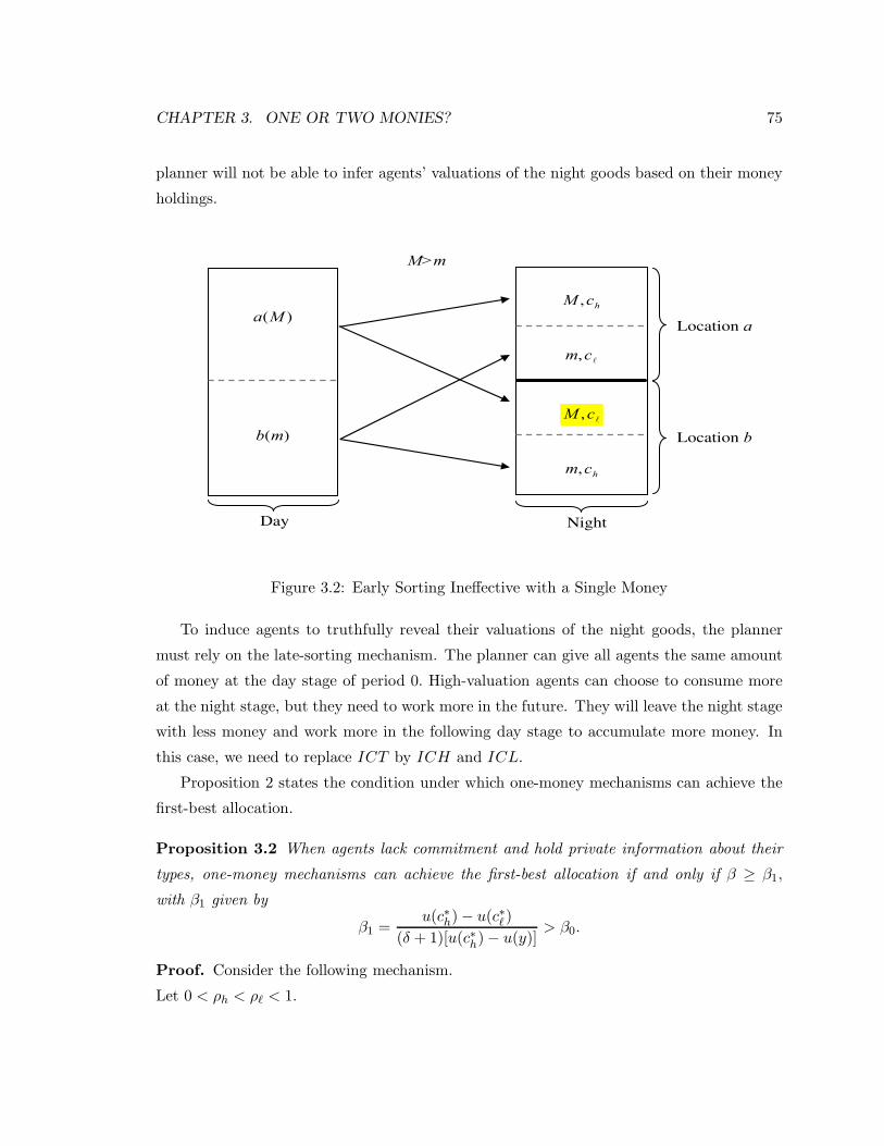
CHAPTER 3. ONE OR TWO MONIES? 75
planner will not be able to infer agents’ valuations of the night goods based on their money
holdings.
hcM ,
cm,
Night
)(Ma
)(mb
Day
Location a
cM ,
hcm,
Location b
M>m
Figure 3.2: Early Sorting Ineffective with a Single Money
To induce agents to truthfully reveal their valuations of the night goods, the planner
must rely on the late-sorting mechanism. The planner can give all agents the same amount
of money at the day stage of period 0. High-valuation agents can choose to consume more
at the night stage, but they need to work more in the future. They will leave the night stage
with less money and work more in the following day stage to accumulate more money. In
this case, we need to replace ICT by ICH and ICL.
Proposition 2 states the condition under which one-money mechanisms can achieve the
first-best allocation.
Proposition 3.2 When agents lack commitment and hold private information about their
types, one-money mechanisms can achieve the first-best allocation if and only if β ≥ β1,
with β1 given by
β1 =u(c∗h) − u(c∗ℓ )
(δ + 1)[u(c∗h) − u(y)]> β0.
Proof. Consider the following mechanism.
Let 0 < ρh < ρℓ < 1.
CHAPTER 3. ONE OR TWO MONIES? 76
At date 0 day stage, the mechanism endows each agent with one unit of money ($).
At date 0 night stage, after preference shocks are realized, the mechanism offers agents
the following choices.
Show 1 $,
use τ∗ good (1 or 2) to exchange for ρℓ $; or
receive τ∗ good (1 or 2) and ρh $.
With this mechanism, non-participants leave with 1 $ and participants leave with more
than 1 $. Participants receiving transfers consume more and leave with lower money bal-
ances; those giving up endowment consume less and leave with higher balances.8
At date 1 day stage, the mechanism offers agents the following options.
Show (1 + ρh) $, use z day good to exchange for (1 − ρh) $;
Show (1 + ρℓ) $, receive z day good and (1 − ρℓ) $.
With this mechanism, all participants leave the stage with 2 units of money and non-
participating agents leave with less than 2 units of money. Participants entering with lower
balances work to earn extra money.
At date 1 night stage, the choices are
Show 2 $,
use τ∗ good (1 or 2) to exchange for ρℓ $; or
receive τ∗ good (1 or 2) and ρh $.
At date t ≥ 2 day stage, the choices are
Show (t + ρh) $, use z day good to exchange for (1 − ρh) $;
Show (t + ρℓ) $, receive z day good and (1 − ρℓ) $.
At date t ≥ 2 night stage, the choices are
Show (t + 1) $,
use τ∗ good (1 or 2) to exchange for ρh $; or
receive τ∗ good (1 or 2) and ρℓ $.
Note that under this mechanism, if an agent skips a stage, his money balance will fall short of
the required balances to participate in all of the following stages. The mechanism effectively
catches non-participants and casts them into perpetual autarky. The individual rationality
conditions thus remain the same as in the case with the record-keeping technology.
The first-best allocation can be achieved if and only if there exists a z such that at (c∗h, c∗ℓ , z),
8Since there is a contemporaneous memory technology, the mechanism can prevent agents from partici-pating more than once.
CHAPTER 3. ONE OR TWO MONIES? 77
ICH, ICL, IRH and IRL are satisfied, or
u(c∗h) − u (c∗ℓ )
2β≤ z ≤
δ[u(c∗h) − u (c∗ℓ )]
2β, (IC)
u(y) − u(c∗ℓ )
β+ W0 − W ∗ ≤ z ≤ W ∗ − W0. (IR)
z is non-empty if and only if
u(c∗h) − u(c∗ℓ )
2β≤ W ∗ − W0,
which can be rearranged as
β ≥u(c∗h) − u(c∗ℓ )
(δ + 1)[u(c∗h) − u(y)]≡ β1.
If follows from δu(c∗h) + u(c∗ℓ ) > (1 + δ)u(y) that β1 > β0.
The one-money mechanism outlined above deals with frictions caused by limited com-
mitment and private information as follows. By rewarding participants with newly issued
money and increasing the money balances required for future participation, the mechanism
effectively catches non-participants and casts them into perpetual autarky. By requiring
previous high-valuation agents to work for previous low-valuation agents at the day stage,
the mechanism induces agents to truthfully reveal private information and signal preferences
by choosing different money balances at the night stage. The first-best allocation can be
implemented if and only if β ≥ β1. When β0 < β < β1, the one-money mechanism cannot
implement the first-best allocation, while the mechanism with a record-keeping technol-
ogy can. In this sense, the one-money mechanism is less powerful in dealing with private
information about types.
3.4.2 Two-Money Mechanisms
Given that one-money mechanisms cannot fully replicate the allocations that are imple-
mentable with a record-keeping technology, we introduce a second money in this subsection
and show that two monies constitute a perfect substitute for the record-keeping technology.
Label the two monies as ”red” and ”green”. Similar to the one-money mechanism, the
two-money mechanism can reward participants with more money balances and effectively
exclude nonparticipants from the mechanism forever. The individual rationality conditions
thus stay the same as in the case with the record-keeping technology.
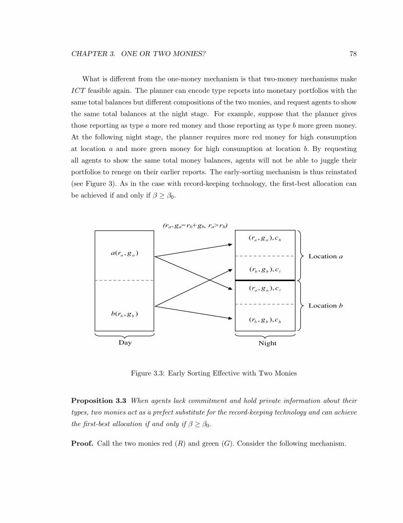
CHAPTER 3. ONE OR TWO MONIES? 78
What is different from the one-money mechanism is that two-money mechanisms make
ICT feasible again. The planner can encode type reports into monetary portfolios with the
same total balances but different compositions of the two monies, and request agents to show
the same total balances at the night stage. For example, suppose that the planner gives
those reporting as type a more red money and those reporting as type b more green money.
At the following night stage, the planner requires more red money for high consumption
at location a and more green money for high consumption at location b. By requesting
all agents to show the same total money balances, agents will not be able to juggle their
portfolios to renege on their earlier reports. The early-sorting mechanism is thus reinstated
(see Figure 3). As in the case with record-keeping technology, the first-best allocation can
be achieved if and only if β ≥ β0.
haa cgr ),,(
cgr bb ),,(
Night
),( aa gra
),( bb grb
Day
Location a
cgr aa ),,(
hbb cgr ),,(
Location b
(ra+ga=rb+gb, ra>rb)
Figure 3.3: Early Sorting Effective with Two Monies
Proposition 3.3 When agents lack commitment and hold private information about their
types, two monies act as a prefect substitute for the record-keeping technology and can achieve
the first-best allocation if and only if β ≥ β0.
Proof. Call the two monies red (R) and green (G). Consider the following mechanism.
CHAPTER 3. ONE OR TWO MONIES? 79
At date 0 day stage, the mechanism asks agents to choose from two monetary portfolios:
1 R or 1 G.
At date 0 night stage, after the shocks are realized, the mechanism offers agents the
following choices.
At location a,
Show R, receive τ∗ good 1 and ρ R, where 0 < ρ < 1;
Show G, use τ∗ good 1 to exchange for ρ R;
At location b,
Show G, receive τ∗ good 2 and ρ G;
Show R, use τ∗ good 2 to exchange for ρ G.
With this mechanism, non-participants leave the night stage with 1 unit of money and
participants leave with more than 1 unit of money. Participants with higher consumption
leave the night stage with a single type of money (i.e., 1 + ρ units of R at location a);
participants with lower consumption leave with two types of money (for example, 1 unit of
G and ρ units of R at location a). All participants exit the night stage with the same total
money balances 1 + ρ.
At date 1 day stage,
Show (1 + ρ) R, use z day output to exchange for (1 − ρ) R;
Show (1 + ρ) G, use z day output to exchange for (1 − ρ) G;
Show R + ρ G, use ρ G to exchange for z day output and 1 R;
Show G + ρ R, use ρ R to exchange for z day output and 1 G.
At date 1 night stage,
At location a,
Show 2 R, receive τ∗ good 1 and ρ R;
Show 2 G, use τ∗ good 1 to exchange for ρ R;
At location b,
Show 2 G, receive τ∗ good 2 and ρ G;
Show 2 R, use τ∗ good 2 to exchange for ρ G.
At date t ≥ 2 day stage,
Show (t + ρ) R, use z day output to exchange for (1 − ρ) R;
Show (t + ρ) G, use z day output to exchange for (1 − ρ) G;
Show t R + ρ G, use ρ G to exchange for z day output and 1 R;
Show t G + ρ R, use ρ R to exchange for z day output and 1 G.
CHAPTER 3. ONE OR TWO MONIES? 80
At date t ≥ 2 night stage,
At location a,
Show (t + 1) R, receive τ∗ good 1 and ρ R;
Show (t + 1) G, use τ∗ good 1 to exchange for ρ R;
At location b,
Show (t + 1) G, receive τ∗ good 2 and ρ G;
Show (t + 1) R, use τ∗ good 2 to exchange for ρ G.
The two-money mechanism described here rewards participants with more money balances,
effectively catches non-participants and bars them from participating in the mechanism
forever. The individual rationality conditions thus stay the same as in the case with the
record-keeping technology.
The two-money mechanism can induce the two types of agents to hold different monetary
portfolios with the same total balances. At the night stages, low-valuation agents will not be
able to falsely claim to be high-valuation agents. For example, suppose that type a choose
to hold red money and type b choose to hold green money at date 0. At the following night
stage, a type a agent at location b is a low-valuation agent and cannot claim to be a high-
valuation agent since he does not have the green money required for higher consumption. We
verify in the following that the two types of agents indeed have the incentive to differentiate
themselves from each other by choosing different monetary portfolios at date 0. Take type
a agents as an example. The expected life-time utility from holding the red money is9
W ar =
1
2
1
1 − β[δu(c∗h) + u(c∗ℓ )],
and the expected utility from holding the green money is
W ag =
1
2
1
1 − β[δu(c∗ℓ ) + u(c∗h)].
It is straightforward that W ar > W a
g so that type a agents prefer holding the red money.
The mechanism outlined above can achieve the first-best allocation if the allocation (ch, cℓ, z)
satisfies ICT , IRH and IRL at (c∗h, c∗ℓ ). As in the case with a record-keeping technology,
the first-best allocation can be achieved if and only if β ≥ β0.
9Note that under the proposed mechanism, agents hold the same color of money while entering all nightstages; they basically make only one type reporting choice when they decide what portfolio to hold at the daystage of period 0. This is why we compare the life-time utilities from holding different monetary portfolios.
CHAPTER 3. ONE OR TWO MONIES? 81
The two-money mechanism induces the two types of agents to hold different monetary
portfolios. Since the two portfolios feature the same total balances, it is impossible to juggle
one’s portfolio to renege on earlier type reports. The early-sorting mechanism (ICT ) is thus
reinstated and two monies provide a perfect substitute for the record-keeping technology.
The introduction of a second money improves welfare when β < β1.10
3.5 Extension to Multi-type-agent Models
In this section, we show that as in Townsend (1987), two monies consist of a perfect
substitute for the record-keeping technology even when there are more than two types
of agents.11 The optimal two-money mechanism is to let different types hold different
combinations of the red and green monies, with all combinations giving the same total
money balances.
There are N < +∞ symmetric locations and N location specific night goods. There
are N types of agents distinguished by their preferences over the night goods. A type
m ∈ 1, 2, ..., N agent derives utility δmnu(cmn) from consuming cmn units of night good
n ∈ 1, 2, ..., N, where δmn = δm−n+I(m<n)N , δ0 > δ1 > δ2 > ... > δN−1 > 0, and
I(m < n) = 1 if m > n and 0 otherwise. For example, type 1 agents derive utility δ0(c)
from goods at location 1, δN−1u(c) from goods at location 2,..., and δ1u(c) from goods
at location N ; type N agents derive utility δ0u(c) from goods at location N, δN−1u(c)
from goods at location 1, ..., and δ1u(c) from goods at location N − 1. See table 1 for an
illustration of the structure of the preferences. The columns represent the types of goods
and the rows represent the types of agents.
During the day, all agents can produce and consume the day good. At night, each agent
is subject to a preference shock and goes to each of the N locations with the same probability
1/N. After agents are relocated, at location n ∈ 1, 2, ..., N, all agents are endowed with y
units of good n, but they differ in their valuations of the good. Agents cannot commit and
agents’ types and thus their valuations of the night goods are private information.
10Note that when β < β0, the first-best allocation cannot be achieved even with a record-keeping technol-ogy. It can be shown that two monies are still a perfect substitute for the record-keeping technology andtwo-money mechanisms strictly improve welfare over one-money mechanisms.
11Kocherlakota and Krueger (1999) also mention that two monies are sufficient in their model which hasonly two types of agents. With indivisible monies, however, more monies will be needed if there are morethan two types of agents.
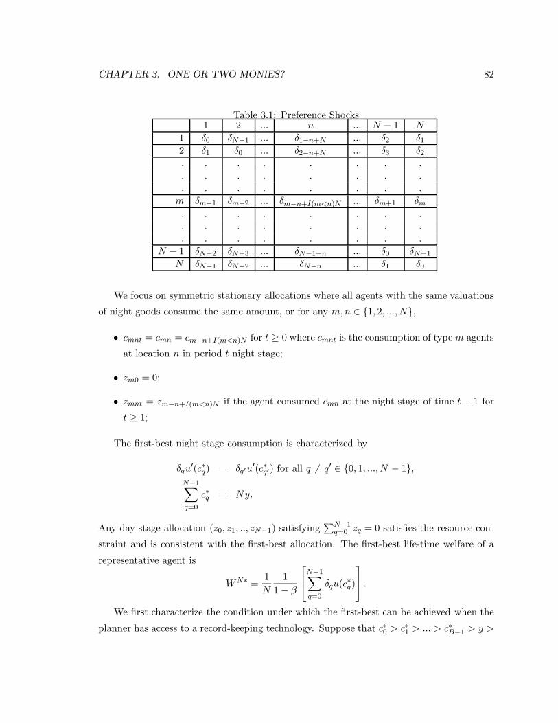
CHAPTER 3. ONE OR TWO MONIES? 82
Table 3.1: Preference Shocks1 2 ... n ... N − 1 N
1 δ0 δN−1 ... δ1−n+N ... δ2 δ1
2 δ1 δ0 ... δ2−n+N ... δ3 δ2
. . . . . . . .
. . . . . . . .
. . . . . . . .
m δm−1 δm−2 ... δm−n+I(m<n)N ... δm+1 δm
. . . . . . . .
. . . . . . . .
. . . . . . . .
N − 1 δN−2 δN−3 ... δN−1−n ... δ0 δN−1
N δN−1 δN−2 ... δN−n ... δ1 δ0
We focus on symmetric stationary allocations where all agents with the same valuations
of night goods consume the same amount, or for any m,n ∈ 1, 2, ..., N,
• cmnt = cmn = cm−n+I(m<n)N for t ≥ 0 where cmnt is the consumption of type m agents
at location n in period t night stage;
• zm0 = 0;
• zmnt = zm−n+I(m<n)N if the agent consumed cmn at the night stage of time t − 1 for
t ≥ 1;
The first-best night stage consumption is characterized by
δqu′(c∗q) = δq′u
′(c∗q′) for all q 6= q′ ∈ 0, 1, ..., N − 1,
N−1∑
q=0
c∗q = Ny.
Any day stage allocation (z0, z1, .., zN−1) satisfying∑N−1
q=0 zq = 0 satisfies the resource con-
straint and is consistent with the first-best allocation. The first-best life-time welfare of a
representative agent is
W N∗ =1
N
1
1 − β
N−1∑
q=0
δqu(c∗q)
.
We first characterize the condition under which the first-best can be achieved when the
planner has access to a record-keeping technology. Suppose that c∗0 > c∗1 > ... > c∗B−1 > y >
CHAPTER 3. ONE OR TWO MONIES? 83
c∗B > ... > c∗N−1 so that at the first-best allocation, B types of agents are borrowers who
consume more than their endowment, and N − B types of agents are lenders who consume
less than their endowment.
To deal with limited commitment, the following 2N individual rationality conditions
must be satisfied: for all q, q′ ∈ 0, 1, ..., N − 1 and q 6= q′,
δqu(cq) + β(−zq + W N ) ≥ δqu(y) + βW N0 ,
−zq + W N ≥ W N0 ,
where
W N =1
N
1
1 − β
N−1∑
q=0
δqu(cq)
and
W N0 =
1
N
1
1 − βu(y)
N−1∑
q=0
δq.
There are two ways to deal with the friction caused by private information. If early-
sorting is used, the following (N2 − N) constraints must be satisfied
1
N
1
1 − β
[
N∑
n=1
δmnu(cmn)
]
≥1
N
1
1 − β
[
N∑
n=1
δmnu(cm′n)
]
,
for all m,m′ ∈ 1, 2, ..., N and m′ 6= m. If late-sorting is used, the following (N2 − N)
constraints must be satisfied
δqu(cq) + β(−zq + W N ) ≥ δqu(cq′) + β(−zq′ + W N ),
for all q 6= q′ ∈ 0, 1, ..., N − 1.
Following the steps in section 3, it can be shown that the ICT s hold at the first-best
allocation. When there is a record-keeping technology, the first-best allocation can be
achieved if and only if
β ≥ βN0 =
∑N−1q=B δq
[
u(y) − u(c∗q)]
∑B−1q=0 δq
[
u(c∗q) − u(y)].
In the absence of a record-keeping technology, one-money mechanisms must resort to
late-sorting to align incentives, and the first-best allocation can be achieved if and only if
β ≥ βN1 =
∑N−1q=1 (N − q)δq
[
u(c∗q−1) − u(c∗q)]
∑N−1q=1 (N − q)δq
[
u(c∗q−1) − u(c∗q)]
+∑N−1
q=0 δq
[
u(c∗q) − u(y)]
≥ βN0 .
CHAPTER 3. ONE OR TWO MONIES? 84
The following proposed mechanism with two monies (R and G) shows that two monies act
as a perfect substitute for the missing record-keeping technology. Two-money mechanisms
improve welfare over one-money mechanisms when β < βN1 .
At the day stage of date 0, the mechanism asks agents to choose from N monetary
portfolios
rm R + (1 − rm) G,
with 0 < rm < 1 for all m ∈ 1, 2, ..., N and rm 6= rm′ for all m 6= m′.
At the night stage of date 0, after the shocks are realized, the planner offers each
agent the following choices.
At location n ∈ 1, 2, ..., N,
Show rm R + (1 − rm) G, get cmn = cm−n+I(m<n)N good n and ε[rn R + (1 − rn) G]
where 0 < ε < minm6=m′∈1,2,...,N
|rm − rm′ |.
The mechanism requires agents to show 1 unit of money to participate in the stage,
and proposes consumption contingent on the composition of monetary portfolios held by
agents. The mechanism rewards participating agents with ε units of money, the composition
of which differs across locations. We restrict ε to ensure that agents of different types and
consuming at different locations exit the night stage with different monetary portfolios.
At the day stage of the t ≥ 1 period,
Show t[rm R + (1− rm) G] + ε[rn R + (1− rn) G], use zmn = zm−n+I(m<n)N day output
and ε[rn R + (1 − rn) G] to exchange for [rm R + (1 − rm) G].
At the night stage of the t ≥ 1 period,
At location n,
Show (t + 1)[rm R + (1− rm) G], get cmn = cm−n+I(m<n)N good n and ε[rn R+ (1− rn)
G].
The two-money mechanism outlined here deals with limited commitment and private
information exactly the same way as the two-money mechanism with two types of agents.
As long as N is finite, we can see that two monies are always a perfect substitute for the
record-keeping technology. If money is indivisible as in Kocherlakota and Krueger (1999),
we will need at least N monies to replace the record-keeping technology when there are N
types of agents.
CHAPTER 3. ONE OR TWO MONIES? 85
3.6 Two Monies as A Perfect Substitute for the Record-
Keeping Technology
In our model’s environment, two monies are sufficient to replace the record-keeping
technology. Townsend (1987) and Kocherlakota (2002) have similar results in different
environments. Here we develop an intuitive argument to show that two monies are always
sufficient as a substitute for the record-keeping technology so there is no need for a third
money.
If money balances are not concealable, there is a one-to-one match between records and
money balances, money balances will thus carry the relevant information into future periods.
When money balances are concealable, however, the one-to-one match will be destroyed since
individuals can change balances by hiding money. Or, the concealability of money balances
makes it possible for individuals to change records to their own benefits. The introduction
of a second money solves the problem by encoding records into different monetary portfolios
with the same total balances and different compositions of the two monies. Agents will not
be able to juggle their monetary portfolios to mimic other portfolios by concealing money.
Note that when money is divisible, it is possible to encode any finite number of records into
different monetary portfolios so a third money will not be needed.
3.7 Conclusion
In this paper, we show in a quasi-linear environment that in the presence of private
information and limited commitment, a second money can potentially improve welfare by
providing an efficient way to pass information across time.
In the absence of a record-keeping technology, monetary mechanisms (with either a
single money or two monies) can effectively deal with limited commitment by rewarding
participants with more money balances and requiring ever increasing money for future par-
ticipation. The individual rationality conditions stay the same as in the case with the
record-keeping technology where defectors are directly caught and forced into perpetual
autarky.
There are two options to deal with private information about preferences. The first is to
induce agents to truthfully report their types before the realization of the preference shocks
and use the information later on to infer agents’ valuations of the night goods. We call
CHAPTER 3. ONE OR TWO MONIES? 86
this early-sorting. The second option is to induce agents to report their valuations after the
realization of the preference shocks, and use the day stage consumption/production to align
the incentives. We call this late-sorting.
Mechanisms with a single concealable money rule out early-sorting. When agents are
patient enough, the late-sorting mechanism effectively aligns the incentive by inducing
agents to leave the night stage with different money balances and produce/consume different
amounts in the following day stage. When agents are not patient enough, the late-sorting
mechanism is not powerful enough to align incentives. The introduction of a second money
permits the early-sorting mechanism and allows agents to signal their preferences by holding
different monetary portfolios (with the same total money balances).
We intend to extend the paper in the following way. In the paper, we take the mechanism
design approach and there is no market in the mechanisms proposed in the paper. In
particular, monies do not circulate as a medium of exchange. We would like to follow
Waller (2007) to see if the allocations can be decentralized with market mechanisms (and
with the help of monetary and fiscal policies). In cases that a second money can enhance
welfare, we can then further investigate whether the second money merely serves as a receipt
or we also require the second money to circulate.
3.8 References
Andolfatto, David (2008), ”The Simple Analytics of Money and Credit in a Quasi-linear
Environment,” manuscript, Simon Fraser University.
Camera, Gabriele, Ben Craig and Christopher J. Waller, (2004), ”Currency Competition in a
Fundamental Model of Money,” Journal of International Economics, 64, pp. 521-544.
Camera, Gabriele and Johannes Winkler, (2003), ”International Monetary Trade and the
Law of One Price,” Journal of Monetary Economics, 50, pp. 1531-1553.
Craig, Ben and Christopher J. Waller, (2004), ”Dollarization and Currency Exchange,”
Journal of Monetary Economics, 51, pp. 671-689.
Kocherlakota, Narayana (1998a), ”The Technological Role of Fiat Money,” Federal Reserve
Bank of Minneapolis Quarterly Review, 22 (3), pp. 2–10.
CHAPTER 3. ONE OR TWO MONIES? 87
Kocherlakota, Narayana (1998b), ”Money is Memory,” Journal of Economic Theory, 81(2),
pp. 232–251.
Kocherlakota, Narayana and Thomas Krueger (1999), ”A Signaling Model of Multiple Cur-
rencies,” Review of Economic Dynamics, 2, pp. 231-244.
Kocherlakota, Narayana (2002). ”The Two-money Theorem,” International Economic Re-
view, 43(2), pp. 333-346.
Lagos, Ricardo and Randall Wright (2005), ”A Unified Framework for Monetary Theory
and Policy Analysis,” Journal of Political Economy, 113(3), pp. 463-484.
Townsend, Robert M. (1987), ”Economic Organization with Limited Communication,” The
American Economic Review, 77(5), pp. 954–971.
Trejos, Alberto and Randall Wright (1995), ”Search, Money, Bargaining, and Prices,” Jour-
nal of Political Economy, 103, 118-141.
Trejos, Alberto and Randall Wright (2001), ”International Currency,” Advances in Macroe-
conomics, Vol 1, Issue 1, Article 3.
Waller, Christopher J. (2007), ”Dynamic Taxation, Private Information and Money,” manuscript,
University of Notre Dame.


