Three Essays on Modeling AgingPopulation

by

Somaieh Nikpoor

Thesis submitted to theFaculty of Graduate and Postdoctoral Studies

In partial fulfillment of the requirementsFor the Ph.D. degree in

Economics

Department of EconomicsFaculty of Social Science

University of Ottawa

© Somaieh Nikpoor, Ottawa, Canada, 2017

Abstract

Chapter 1: Interregional Transfers through Public Pension in Canada

In this chapter, I build a regional computable general equilibrium model with an over-

lapping generations (OLG) structure of the Canadian economy to analyse population aging

dynamics and public pensions. Canada is divided into three regions: Atlantic, Quebec and

Rest of Canada (ROC). The impact of population aging is investigated on each of three

regions’ pension systems. The results confirm that as a result of aging all regions are

affected negatively if they choose to have an independent pension system. Under a joint

pension system most of the pressure of the provision of the pension system is on the ROC.

Atlantic region benefits the most from a joint pension plan as the implicit funds flow from

ROC to Atlantic region. Quebec benefits from having its own program, but the benefits

disappear slowly in future years.

Chapter 2: Age-Variable Rate of Time Preference in CGE-OLG Model

Contrary to the mainstream studies in the area of intertemporal optimization that

assume a constant rate of time preference over individuals’ life cycles, in this chapter I

propose a new approach to measure the rate of time preference by assuming that the rate

of time preference evolves by age. I construct an overlapping generations model (OLG) and

calibrate rate of time preference. The age-variable rate of time preference would permit to

capture many other elements that affect the life cycle profile of consumption as observed

in the data. The results show that rate of time preference exhibits three phases and is

different for young versus old.

ii

Chapter 3: Computing Demographic Change Simulation under Constant

and Age-variable Rate of Time Preference

This chapter simulates the impact of an aging population on various macroeconomic

variables and calculates the cohort welfare as well as social welfare. The outcomes from

simulations are dependent on the choice of rate of time preference as well as the structure

of the model. The results in this chapter provide a new approach to determining the

impact of aging population. The choice of a realistic rate of time preference, which allows

its variability by age, affects the cohort welfare noticeably.

iii

Acknowledgement

Firstly, I would like to express my sincere gratitude to my supervisor Professor Marcel

Mrette for the continuous support of my Ph.D study, for his patience, motivation, and

immense knowledge. His guidance helped me throughout my research and writing of this

thesis. I would like to thank him for encouraging my research and for allowing me to grow

as a researcher.

I would also like to thank Professor Luc Savard, Professor Michel Demers, Professor

Nguyen Van Quyen and Professor Yazid Dissou for serving as my committee members. I

also want to thank them for letting my defense be an enjoyable moment, and for their

brilliant comments and suggestions.

My heartfelt thanks also go to Professor Rose Anne Devlin, Professor Serge Coulombe

and Professor Lilia Karnizova. I appreciate their helpful guidance and mentorship from

which I have benefited enormously.

Completing this work would have not been possible without the help and support of

my friends and colleagues from the University of Ottawa. Hence, I would like to thank

Golnaz Sedigh, Rashid Nikzad, Sophie Benard, Catherine Millot, Jeffrey Peter, Faisal Arif,

Rizwana Alamgir Arif, Ida Liu, Lila Kayembe and Olayinka Williams, JoAnne St-Gelais

and Forough Seifi.

I deeply appreciate the support I received from Elena Tipenko, Olga Anglinova, Steven

Gonzalez, Marie Josee Dorion, Imran Ahmed and Fares Said for their encouragement when

I needed it most.

iv

A big thank you to my great friends Marjan Soltanzedah and Reza Farzi for their

generous support, constructive advice and positive vibes over the past couple of years. I

am indebted to them for their help.

Last but not the least, I would like to thank my family: my loving mom and dad, my

two wonderful sisters and my amazing aunt for their moral support while I was writing

this thesis and throughout my life in general.

v

I dedicate this thesis to mom and dad. For their endless love, support and encouragement.

Thank you for always believing in me.

vi

Table of Contents

List of Tables x

List of Figures xi

Introduction to Thesis . . . . . . . . . . . . . . . . . . . . . . . . . . . . . . . . 1

1 Interregional Transfers through Public Pension in Canada 3

1.1 Introduction . . . . . . . . . . . . . . . . . . . . . . . . . . . . . . . . . . . 3

1.2 Income Security System in Canada . . . . . . . . . . . . . . . . . . . . . . 6

1.2.1 Reforms to the Pension Plan . . . . . . . . . . . . . . . . . . . . . . 8

1.3 Population Dynamics in Canada . . . . . . . . . . . . . . . . . . . . . . . . 11

1.4 Review of Relevant Literature . . . . . . . . . . . . . . . . . . . . . . . . . 18

1.4.1 Population Dynamics and the Economy’s Performance . . . . . . . 18

1.4.2 Population Dynamics and Pension Plan . . . . . . . . . . . . . . . 20

1.4.3 Population Dynamics, Pension Plan and Multi-region Model . . . . 23

1.5 Model . . . . . . . . . . . . . . . . . . . . . . . . . . . . . . . . . . . . . . 26

1.5.1 Firm Behaviour . . . . . . . . . . . . . . . . . . . . . . . . . . . . . 26

1.5.2 Household Behaviour . . . . . . . . . . . . . . . . . . . . . . . . . . 30

1.5.3 Pension . . . . . . . . . . . . . . . . . . . . . . . . . . . . . . . . . 36

1.5.4 Government . . . . . . . . . . . . . . . . . . . . . . . . . . . . . . . 38

1.5.5 Market Clearing Condition . . . . . . . . . . . . . . . . . . . . . . . 41

vii

1.6 Data and Calibration . . . . . . . . . . . . . . . . . . . . . . . . . . . . . . 44

1.6.1 Demographic Structure . . . . . . . . . . . . . . . . . . . . . . . . . 45

1.6.2 Calibration . . . . . . . . . . . . . . . . . . . . . . . . . . . . . . . 48

1.7 Simulation . . . . . . . . . . . . . . . . . . . . . . . . . . . . . . . . . . . . 49

1.7.1 Implicit Transfers Across Regions . . . . . . . . . . . . . . . . . . . 53

1.8 Conclusion . . . . . . . . . . . . . . . . . . . . . . . . . . . . . . . . . . . . 57

1.9 Appendix for Chapter 1 . . . . . . . . . . . . . . . . . . . . . . . . . . . . 59

1.9.1 List of variables . . . . . . . . . . . . . . . . . . . . . . . . . . . . . 59

1.9.2 List of parameters . . . . . . . . . . . . . . . . . . . . . . . . . . . 61

2 Age Variable Rate of Time Preference in OLG-CGE Model 63

2.1 Introduction . . . . . . . . . . . . . . . . . . . . . . . . . . . . . . . . . . . 63

2.2 Review of Relevant Literature . . . . . . . . . . . . . . . . . . . . . . . . . 66

2.2.1 Time Preferences and Natural Selection . . . . . . . . . . . . . . . . 69

2.2.2 Personality Traits and Time Preferences . . . . . . . . . . . . . . . 73

2.2.3 Experimental Studies . . . . . . . . . . . . . . . . . . . . . . . . . . 77

2.3 Model Description . . . . . . . . . . . . . . . . . . . . . . . . . . . . . . . 82

2.3.1 Firm Behaviour . . . . . . . . . . . . . . . . . . . . . . . . . . . . . 82

2.3.2 Household Behaviour . . . . . . . . . . . . . . . . . . . . . . . . . . 82

2.3.3 Pension . . . . . . . . . . . . . . . . . . . . . . . . . . . . . . . . . 84

2.3.4 Government . . . . . . . . . . . . . . . . . . . . . . . . . . . . . . . 84

2.3.5 Market Clearing Condition . . . . . . . . . . . . . . . . . . . . . . . 85

2.4 Calibration . . . . . . . . . . . . . . . . . . . . . . . . . . . . . . . . . . . 86

2.4.1 Data . . . . . . . . . . . . . . . . . . . . . . . . . . . . . . . . . . . 86

2.4.2 Demographic Structure . . . . . . . . . . . . . . . . . . . . . . . . . 87

2.4.3 Calibration Procedure . . . . . . . . . . . . . . . . . . . . . . . . . 88

2.5 Two Calibration Approaches . . . . . . . . . . . . . . . . . . . . . . . . . . 97

2.6 Calibration Procedure . . . . . . . . . . . . . . . . . . . . . . . . . . . . . 101

viii

2.6.1 First Calibration Procedure . . . . . . . . . . . . . . . . . . . . . . 102

2.6.2 Second Calibration Procedure . . . . . . . . . . . . . . . . . . . . . 103

2.7 Calibration Results . . . . . . . . . . . . . . . . . . . . . . . . . . . . . . . 106

2.7.1 Calibration Results for Approach 1 . . . . . . . . . . . . . . . . . . 106

2.7.2 Calibration Results for Approach 2 . . . . . . . . . . . . . . . . . . 107

2.7.3 Sensitivity Analysis . . . . . . . . . . . . . . . . . . . . . . . . . . . 115

2.8 Conclusion . . . . . . . . . . . . . . . . . . . . . . . . . . . . . . . . . . . . 118

2.9 Appendix for Chapter 2 . . . . . . . . . . . . . . . . . . . . . . . . . . . . 120

3 Computing Demographic Change Simulation under Constant and Age-variable Rate of Time Preference 121

3.1 Introduction . . . . . . . . . . . . . . . . . . . . . . . . . . . . . . . . . . . 121

3.2 Model Structure . . . . . . . . . . . . . . . . . . . . . . . . . . . . . . . . . 126

3.2.1 Firm Behaviour . . . . . . . . . . . . . . . . . . . . . . . . . . . . . 126

3.2.2 Household Behaviour . . . . . . . . . . . . . . . . . . . . . . . . . . 128

3.2.3 Pension . . . . . . . . . . . . . . . . . . . . . . . . . . . . . . . . . 132

3.2.4 Government . . . . . . . . . . . . . . . . . . . . . . . . . . . . . . . 133

3.2.5 Equilibrium Condition . . . . . . . . . . . . . . . . . . . . . . . . . 134

3.3 Simulation . . . . . . . . . . . . . . . . . . . . . . . . . . . . . . . . . . . . 135

3.3.1 Baseline Simulation . . . . . . . . . . . . . . . . . . . . . . . . . . . 135

3.3.2 Welfare Effect . . . . . . . . . . . . . . . . . . . . . . . . . . . . . . 142

3.4 Conclusion . . . . . . . . . . . . . . . . . . . . . . . . . . . . . . . . . . . . 149

3.5 Appendix for Chapter 3 . . . . . . . . . . . . . . . . . . . . . . . . . . . . 151

APPENDICES 154

References 154

ix

List of Tables

1.1 Projected Old-age Dependency Ratio . . . . . . . . . . . . . . . . . . . . . 47

1.2 Calibration Results . . . . . . . . . . . . . . . . . . . . . . . . . . . . . . . 49

1.3 Contribution Rates for Three Scenarios . . . . . . . . . . . . . . . . . . . . 51

1.4 Total Contribution for Three Scenarios, Using 2013-2014 Data, $Billions . 54

2.1 Social Accounting Matrix, United Kingdom, £mil, 2010 . . . . . . . . . . . 87

2.2 Labour Force Participation and Productivity Profile . . . . . . . . . . . . . 91

2.3 Intertemporal Elasticity of Substitution . . . . . . . . . . . . . . . . . . . . 116

2.4 Asset Holdings for Approach 2 . . . . . . . . . . . . . . . . . . . . . . . . . 120

3.1 Value of Model Parameters . . . . . . . . . . . . . . . . . . . . . . . . . . . 136

3.2 Survival Rates . . . . . . . . . . . . . . . . . . . . . . . . . . . . . . . . . . 152

3.3 Simulation Results for Both Models . . . . . . . . . . . . . . . . . . . . . . 153

x

List of Figures

1.1 Population Growth for Regions, Decade Yearly Average . . . . . . . . . . . 12

1.2 Age Pyramid for Canada . . . . . . . . . . . . . . . . . . . . . . . . . . . . 13

1.3 Proportion of Persons Aged 65 Years and Over and Children aged 14 Yearsand Less, Canada, 1971 to 2031 . . . . . . . . . . . . . . . . . . . . . . . . 14

1.4 Dependency Ratio . . . . . . . . . . . . . . . . . . . . . . . . . . . . . . . 15

1.5 Proportion of Age Groups in Total Population . . . . . . . . . . . . . . . . 17

1.6 Proportion of Persons Aged 65 Years and Over and Children Aged 14 Yearsand Less in Canada, 1950-2100 . . . . . . . . . . . . . . . . . . . . . . . . 46

2.1 Earning Profile . . . . . . . . . . . . . . . . . . . . . . . . . . . . . . . . . 92

2.2 Consumption Path, r > ρ . . . . . . . . . . . . . . . . . . . . . . . . . . . 94

2.3 Consumption Path, r < ρ . . . . . . . . . . . . . . . . . . . . . . . . . . . 95

2.4 Consumption Path, r = ρ . . . . . . . . . . . . . . . . . . . . . . . . . . . 95

2.5 Per Capita Consumption, Private and Public by Sector, United States, 2003 99

2.6 Per Capita Consumption, Private and Public by Sector, Canada, CAD $,2006 . . . . . . . . . . . . . . . . . . . . . . . . . . . . . . . . . . . . . . . 100

2.7 Per Capita Consumption, Private and Public by Sector, Germany, 2003 . . 100

2.8 Per Capita Private Consumption, Slovenia, 2014 . . . . . . . . . . . . . . . 101

2.9 Distribution of Consumption from NTA . . . . . . . . . . . . . . . . . . . . 104

2.10 Approach 1: Consumption and Labour Income Age Profile . . . . . . . . . 107

2.11 Approach 2: Consumption and Labour Income Age Profile . . . . . . . . . 108

xi

2.12 Interest Rate and Calibrated Rate of Time Preference . . . . . . . . . . . . 109

2.13 Rate of Change of Time Preference . . . . . . . . . . . . . . . . . . . . . . 111

2.14 Asset Holdings . . . . . . . . . . . . . . . . . . . . . . . . . . . . . . . . . 114

2.15 Calibrated Rate of Time Preference Response to Exogenous Shocks . . . . 115

3.1 Cohort Share in Total Population . . . . . . . . . . . . . . . . . . . . . . . 137

3.2 Saving Levels for Both Models for Selected Years . . . . . . . . . . . . . . 140

3.3 Baseline Simulation for Model with Age-variable ρ . . . . . . . . . . . . . . 141

3.4 Baseline Simulation for Model with Constant ρ . . . . . . . . . . . . . . . 142

3.5 Percentage Change in Cohort Welfare due to Demographic Transition . . . 144

3.6 Cohort Welfare Levels due to Demographic Transition . . . . . . . . . . . . 145

3.7 Percentage Change in Social Welfare due to Demographic Transition . . . . 148

xii

Introduction to Thesis

As people are living longer and baby-boomers are retiring, we observe significant demo-

graphic changes in many countries of the world. This represents important challenges for

economic policy. Aging of the population is expected to affect economic growth and many

other issues, including intergenerational welfare, the ability of states to provide resources

for elderly and international trade. It is crucial for better policy decisions to be able to

develop appropriate models on demographic changes in order to assess properly the impact

of aging populations.

The purpose of this thesis is to contribute to the compelling picture of the impact of

population aging on economic performance. Given the enormous breadth of issues that ag-

ing population generally encompass, in the present context, I narrow down the horizon by

focusing on issues relevant to modeling the demographic changes in an overlapping gener-

ations (OLG) framework. OLG models are considered the most appropriate to investigate

demographic changes since it takes into consideration the age of the representative agents.

In chapter one, I begin by developing an OLG model to investigate the impact of aging

on public pension in Canada. A considerable share of seniors approach their retirement

over the next few decades, while the share of people aged less than 30 years old, will drop.

1

This will put pressure to the provision of the pension program. Demographic changes are

not the same across Canadian provinces. Atlantic Provinces have higher share of elderly

population compared to the rest of the Canada. Quebec has its own pension plan. Thus,

I focus on this issue by dividing Canada into three regions and develop a multi-region

Computable General Equilibrium (CGE) with OLG framework. The results derived from

this exercise highlight the importance of developing a multi-region model to analyze aging

and pension in Canada.

In chapter two of this thesis, I develop an approach to calibrate OLG models with

the rate of time preference allowed to vary by age. In the conventional calibration of

the discounted utility function, the evolution of consumption over life cycle is derived

as a function of the inter-temporal elasticity of substitution, the market interest rate,

and the rate of time preference. A typical assumption is to impose a constant rate of

time preference. This implies upward sloping consumption profile (if the rate of interest

is larger than rate of time preference). Recent empirical studies by National Transfer

Accounts (NTA) have demonstrated that the age profile of consumption is bell shaped.

This permits for new calibration procedure in which the rate of time preference varies by

age. The advantage of the new procedure is that it respects consumption behavior observed

in data. By letting the rate of time preference to vary by age, this chapter provides a new

calibration procedure that satisfies life-cycle profiles observed in the data.

In chapter three of this thesis, long-run impact of aging population is simulated, using

the calibration results obtained from the innovative approach developed in chapter two.

Results derived from simulating an OLG model shows that the impact of aging population

is sensitive to the choice of rate of time preference.

2

Chapter 1

Interregional Transfers throughPublic Pension in Canada

1.1 Introduction

Over the next few decades there will be significant demographic changes in Canada. A

considerable share of seniors approach their retirement, while the share of people aged

less than 30 years old will drop. This demographic change will put pressure on pension

plans for many years to come. This issue has generated debate over the feasible reforms

for pension plans (Baldwin [10], Baldwin [12], Baker et al. [9]). This chapter’s objectives

are twofold: first, to investigate and measure the impact of population aging on Canada’s

public pension contribution rate in a multi-regional computable general equilibrium model,

second, to measure the implicit transfers of resources from the west part of Canada to the

east, generated by the asymmetric population dynamic. In addition, I estimate the implicit

cost or benefit for Quebec for having its own pension plan. In this model Canada is divided

into three regions: Atlantic, Quebec and Rest of Canada (ROC). The population is aging

3

faster in the Atlantic Provinces and in Quebec. Atlantic and ROC retirees receive benefits

from the Canadian pension plan (CPP), but Quebec pension benefits are paid under the

Quebec pension plan (QPP).

While there are some studies that investigate the implications of the aging population

for pension plans, there are no studies that have taken into consideration the two sepa-

rate pension plans, in Canada’s income security system. Since population dynamics are

different across Canadian provinces, the consequences of the aging population will differ.

Heterogeneity in the composition of the population (young versus old) across Canada’s

regions has a critical role in the impact of pension reforms and speed of the population

aging. In the presence of regional differences, there exist diverse regional effects based on

the economic and demographic structures. Wage, employment and productivity effects of

any reforms across regions may not be the same as those observed at the national level.

There are transfers of implicit funds from provinces with implicit pension surplus to

those with implicit pension deficit under the common pension plan. I use a general equilib-

rium model with an overlapping generations (OLG) structure to run three sets of simula-

tions to examine the impact of population dynamics. First, I consider the current situation

in which ROC and Atlantic share the same pension system, while Quebec has its own plan.

In the second scenario, I assume that one pension plan exists for all regions. In the third

scenario, I assume that each region has its own pension plan.

The structure of this chapter is as follows: in section 1.2, I briefly review the income

security system in Canada and the previous reforms. In section 1.3, I describe the popu-

lation dynamics and projections for Canada over the next few decades. In section 1.4, I

4

review the relevant literature. In sections 1.5 and 1.6, I present the model and the required

data and in section 1.7, I discuss the main results concerning the overall dynamic effects

of population aging in the two scenarios. Section 1.8 concludes.

5

1.2 Income Security System in Canada

The national pension system of Canada is primarily an extension of the welfare state

from the 1950s to the 1970s (Beland et al. [19]) 1. Canada’s income security system has

three pillars (Horner [71])2. The first pillar is a flat benefit (Old Age Security) with a

supplement (Guaranteed Income Supplement (GIS)) and is financed through general tax

revenues. The eligibility age for receiving the OAS is 65 years old for Canadians who meet

residence requirements 3. GIS is an income-tested supplement that is allocated to people

who do not receive any income except for the OAS. For income received from sources other

than OAS, the GIS will be ”taxed away”.

The second pillar is the Canada/Quebec pension plans (CPP/QPP), which are income-

related and employment-based pensions. CPP and QPP are the outcome of long bargaining

between the federal government and all ten provinces. It was Quebec’s campaign for

”greater provincial autonomy” that led to the creation of two separate plans that are

highly coordinated. Both plans are financed by employees, employers and those who are

self-employed. People aged between 18 and 70 who have an income that exceeds the

minimum level of earnings contribute to the plan. CPP/QPP contribution rate is 9.9

1The structure of the national pension system of the 60’s takes root in legislative procedures that dateback as far as the 1920s. The first national pension legislation, the Old Age Pension Act (OAP), waslegislated in 1927 (Beland et al. [19]). It assigned 20 dollars to each Canadian over the age of 70. Withtime, legislatures evolved, and in 1951, the Old Age Security Act extended the benefit to 40 dollars whilethe Old Age Assistance Act (OAS) lowered the admissibility age to 65. The latter remained the statusquo until 1970. By the 1980s, OAS along with GIS could provide an ”income floor equal to 50 percent ofaverage earnings for an elderly couple and 31 percent for a single individual” (Beland et al. [19]).

2Contribution rate of employers and employees is 4.95 percent each. Self-employed workers pay thefull 9.9 percent.

3Since 1989, OAS recipients with income above a threshold ($66,733 in 2010) are exposed to a specialtax (Baldwin [10]).

6

percent of earnings between $3,500 dollars and the year’s maximum pensionable earnings

4. The benefit payment is 25 percent of the average monthly income (up to Year’s Maximum

Pensionable Earning (YMPE)) during the contributions years (from age 18 to retirement),

with allowance for some years of low earnings to be dropped from the average. Benefit

payments are adjusted to changes in the CPI (Consumer Price Index). The minimum age

for eligibility for CPP/QPP benefits dropped from 68 to 65 between 1966 and 1970. Since

1987, benefits can be accessed at age 60 5; however, benefit payments are reduced by 0.5

percent per month between the age at which a person begins receiving benefits and age 65

6. CPP/QPP benefits, including survivor and disability benefits, were paid to 7.3 million

people in December 2010 [Horner [71]].

The third pillar of Canada’s income security system is workplace pension and savings

plans (Registered pension plans (RPPs), Registered Retirement Saving Plans (RRSPs)).

Together, these three pillars formed the national pension system at the end of 1960.

The pension plan was established to supplement income after retirement and aims to

replace approximately 25% of pre-retirement earnings. People aged 18 and older contribute

to the plan7. The CPP was initially established as a PAYG (Pay as you go) plan with a

small reserve and with an employer-employee contribution rate of 3.6%. Since the early

1970s, numerous changes have been made in CPP/QPP; however, reforms made in the late

4YMPE, set at $48,300 in 2011, Horner [72].5In the 2012 government budget, OAS benefits eligibility age in Canada was raised from 65 to 67,

starting progressively in year 2023 (HRSDC [74], Budget [32]).6From 2011 to 2013 the government will gradually increase the percentage from 0.5 percent per month

to 0.7 percent. So, if the contributors delay the receipt of their CPP until age 70, the amount receivablewill be 42% more than the amount taken at age 65 (HRSDC [73]).

7Except for people whose earnings are less than the Year’s Basic Exemption (YBE), members of certainreligious groups.

7

1990s had the most significant impact. These changes transformed the pension plan from

a PAYG system to a hybrid of PAYG financing and full funding 8.

In the next section, I briefly review the main pension reforms during the last few

decades.

1.2.1 Reforms to the Pension Plan

The so called ”great-pension-reform” occurred between the mid 1970s and the early 1980s

and took place during two periods: first, from 1984 to 1993 and second, since 1993 (Beland

et al. [19]). The major concern was the expansion of the second tier of the pension plan;

however, in both periods, the flat part of the pension (OAS) was targeted. By 2001, less

than 5 percent of the elderly were affected by the reforms introduced in 1989.

In 1993, there were concerns about the deficit and demographic issues, which made the

Liberals create five principles to reform the pension plan, but no changes were made to

CPP/QPP. Eventually, after the publication of the Fifteenth Actuarial Report of CPP in

1995, it became clear that if the contributions did not change by 2015, CPP would not

collect enough revenue to pay all the benefits and the contribution rate must increase to

14.2% by 2030. In response to this issue, the governing Liberals initiated a consultative

process to reform the pension plan.

In February 1996, the Ministry of Finance published a joint report evaluating the

”long-term financial” situation of CPP and setting the agenda for consensual reform. This

8In the Actuarial Report of 1997, it was called ”steady-state funding”.

8

consultation aimed to review the CPP by federal and provincial governments. At the same

time, the government of Quebec was conducting its own consultancy concerning QPP.

In November 1996, following the consultation between the federal government and

provincial governments, a joint report was published which contained nine principles re-

garding reforming the CPP (Beland et al. [19]). Among them was the creation of the CPP

fund to ensure a more efficient fund management. Investing the CPP fund was a response

to the existence of the Caisse de Depot et Placement du Quebec, which is a provincial

investment board that has successfully invested QPP’s money in equities since the 1960s.

In February 1997, new CPP legislation was proposed by the Ministry of Finance. The

new reforms increased CPP contributions from 5.6 to 9.9 by 2003, in order to accumulate

funds. The fund value is equal to two years of benefits. The CPP Investment Board was

created in order to invest surplus reserve funds in diversified investment portfolios.

Over the last decade, the federal government and the four provinces of Alberta, British

Columbia, Ontario and Nova Scotia have started important pension reviews. In November

2009, the government of Ontario released the report of the Ontario Expert Commission

on Pension (OECP), providing a number of recommendations for improving the pension

system. Soon after the release of the OECP, the Alberta/British Colombia Joint Expert

Panel on Pension Standards (JEPPS), released a report providing recommendations to im-

prove the pension standards in order to facilitate establishment of an independent, ”widely

accessible”, ”privately-run” and voluntary Defined Contribution (DC) pension plan to deal

with the problem of low pension coverage. In January 2009, Nova Scotia’s Pension Review

recommended a model similar to the JEPPS model.

9

In 2009, the Ministry of Finance of the government of Ontario provided a report con-

taining the options available for pension plan reforms (Baldwin [10]). Since then, several

reports on pension plan reform options have been released either by federal or provincial

governments or by private research institutions, which accentuate the necessity for pension

plan reforms (Baldwin [12], Horner [72], Baldwin [11]).

At the time of the inception of the pension plan, due to the economic conditions, a

PAYG pension plan was appropriate and the total contribution of the workforce was suf-

ficient to cover the pension benefits; however, since then demographic conditions have

changed. An ever decreasing mortality rate and a declining fertility rate manifest them-

selves in increasing the percentage of the elderly in the total population. Thus, with a

growing share of the population 65 years old and over, the cost of the PAYG pension sys-

tem will continue to increase. In order to ensure the sustainability of the pension plan for

future generations, including changes in the population structure should be an important

part of any pension plan reform. The next section describes the demographic dynamics in

Canada over the past four decades.

10

1.3 Population Dynamics in Canada

On July 1, 2012, Canada’s population was estimated at 34,880,500 with a 1.1 percent

increase compared to the previous year. This rate is slightly larger than the average

growth rate for the past 30 years (1%). The highest population growth rate that Canada

experienced was 1.8 percent in 1988/1989. The variation of the growth rate for the past

30 years was between 0.8 and 1.2 percent.

Population growth varies across Canada’s provinces and territories. Figure 1.1 shows

the estimated and projected growth rate across Canada’s three regions. As is shown, the

population growth is lower in the Atlantic provinces and Quebec compared to the rest of

the Canada. The projected growth rate will become negative for Quebec in 2040 and for

the Atlantic provinces in early 2025. Compared with the ROC, population growth steeply

declines in Quebec and the Atlantic provinces. In Quebec, the growth rate moved from

0.7 in 1999 to 0.3 in 2011. In the past 30 years, the population growth rate of the western

provinces has been higher than the Atlantic provinces and Quebec. The decline in the birth

rate and the mortality rate and, the increase in life expectancy are contributing factors to

the lower growth rate in Canada.

Figure 1.2 shows the population pyramid for Canada as of July 1, 2010. The large

cohort of baby boomers, born between 1946 and 1965, are currently in the 45 to 64 year

age range. By comparing the 2010 pyramid to that of 1971, we can see the progression of

the baby boomers through the age structure. This cohort makes the population pyramid

more rectangular-shaped. The lower birth rate has narrowed the lower part of the pyramid,

which clearly shows low fertility at the base of the pyramid and increasing life expectancy

11

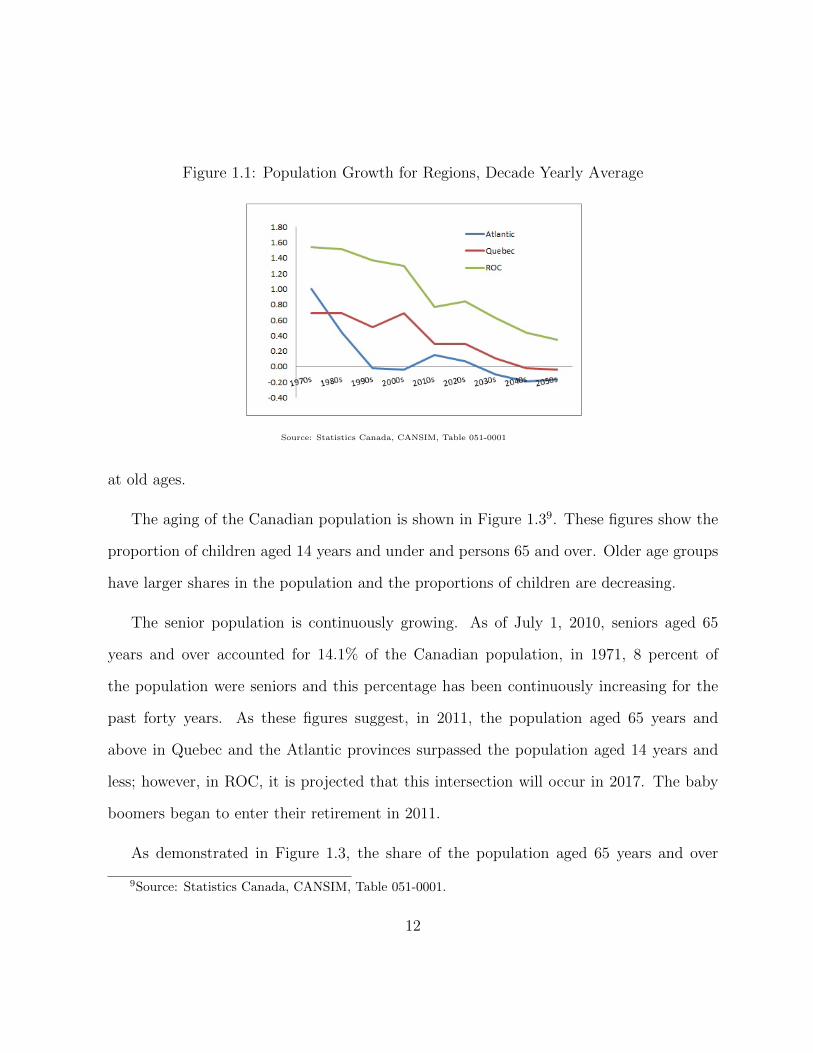
Figure 1.1: Population Growth for Regions, Decade Yearly Average

Source: Statistics Canada, CANSIM, Table 051-0001

at old ages.

The aging of the Canadian population is shown in Figure 1.39. These figures show the

proportion of children aged 14 years and under and persons 65 and over. Older age groups

have larger shares in the population and the proportions of children are decreasing.

The senior population is continuously growing. As of July 1, 2010, seniors aged 65

years and over accounted for 14.1% of the Canadian population, in 1971, 8 percent of

the population were seniors and this percentage has been continuously increasing for the

past forty years. As these figures suggest, in 2011, the population aged 65 years and

above in Quebec and the Atlantic provinces surpassed the population aged 14 years and

less; however, in ROC, it is projected that this intersection will occur in 2017. The baby

boomers began to enter their retirement in 2011.

As demonstrated in Figure 1.3, the share of the population aged 65 years and over

9Source: Statistics Canada, CANSIM, Table 051-0001.

12

Figure 1.2: Age Pyramid for Canada

Source: Statistics Canada,2010, Annual Demographic Estimates: Canada, Provinces andTerritories, No 91-215x.

in Quebec and the Atlantic provinces will increase from 15% in 2011 to 25% and 27%

respectively in 2031; however, in the ROC, it is projected to increase from 15% in 2017 to

22% in 2031. In 2011, the share of people aged 65 years and above continues to be lower

than those aged 14 years and less for the ROC. The share of this group was the same for

all three regions in 1971. The age gap between these two age groups increases faster for

Quebec and the Atlantic provinces compared to the ROC.

The economic implications of the population dynamics appear in the old age Depen-

dency Ratio (DR). Figure 1.4 shows the projected old age dependency ratio for Canada’s

three regions. The old age DR is the number of persons aged 65 years and above, over

persons aged between 15 and 64. All of Canada’s three regions have almost the same DR

in 2006; however, in 2031, there is a large difference in the DR among regions. Between

2006 and 2031, the DR triples for the Atlantic region and increases more than 100% in

13

Figure 1.3: Proportion of Persons Aged 65 Years and Over and Children aged 14 Yearsand Less, Canada, 1971 to 2031

(a) Atlantic (b) Quebec

(c) ROC

14

Figure 1.4: Dependency Ratio

Source: Statistics Canada, CANSIM, Table 051-0001

Quebec. In the ROC, it only increases about 60%. The DR provides an insight into the

future financial burden for elderly pensions. The increase in the senior population relative

to the working-age population has implications for Canada’s economy.

A high dependency ratio is likely to reduce productivity growth. Since the retired

population will make a bigger share of the population, the productive share of the labour

market will diminish and lead to lower economic growth. In a PAYG pension system, the

seniors’ pension benefits have to be financed by the working age population. The increase

in the senior population relative to the working age population will put pressure on the

provision of pension benefits.

As of July 1, 2010, the working-age population, aged 15 to 64 years, accounted for

69.4% of the total population of Canada. This proportion was 62.7% in 1971. As Figure

15

1.410 shows, Quebec and the Atlantic provinces have a higher dependency ratio compared

to ROC and it is expected to increase substantially over the next 20 years. The increase

is less dramatic in the ROC. The increase is projected to be 140 percent in the Atlantic

provinces, 110 percent in Quebec, and 100 percent in the ROC. As of July 1, 2010, people

aged 80 years and over in Canada represent 3.9% of the total population. By the year

2031 this will double and by 2061, the end of the most recent projection, there could be

5.1 million people aged 80 and above.

The structure of the working population is also very crucial. As Figure 1.511 shows, the

share of the younger part of the working population, people aged between 15 and 24, has

been decreasing since the 1990s which also affects the share of the working age population

between 25 and 64. In the same period the share of the old age group is increasing. There

is an increase in the ratio of those aged 15 to 24 years old in all three regions when the

baby boomers enter the labour market. This increase is later shifted to the second part

of the working age population, people aged 25 to 64. Since 2005, in the Atlantic region,

the share of people aged 25 to 64 is decreasing rapidly while for Quebec it is decreasing

gradually since 1995. In ROC, the decrease has started since 2012.

The economic role and the contributions of people vary by age. Adults (people aged

between 25 to 64) are net producers and savers and the elderly are net consumers. The

declining share of individuals in the labour force has discouraging effects on productivity

growth. Population aging could affect not only labour supply but also capital deepening

and total factor productivity, because economic output will be achieved by a contracted

10Statistics Canada, CANSIM, Table 051-0001.11Statistics Canada, CANSIM, Table 051-0001.

16

Figure 1.5: Proportion of Age Groups in Total Population

(a) Atlantic (b) Quebec

(c) ROC

17

and older labour force.

1.4 Review of Relevant Literature

1.4.1 Population Dynamics and the Economy’s Performance

Investigating the impact of population dynamics in an economy was first studied in the

Life Cycle model by Modigliani [97]. Modigliani [97] probes the relationship between

private and public saving with population structure. Since then, many researchers study

the link between aggregate saving and demographic structure (Attanasio and Weber [5],

Graham et al. [59], Masson et al. [93]). Numerous studies have investigated the impact

of population structure and its dynamics on different aspects of an economy, such as

government spending, tax revenue, economic growth and labour market (Leibfritz et al.

[90], Disney [39], Fougere and Merette [54], Fougere et al. [53]).

Leibfritz et al. [90] explore the effects of demographic changes on government budget

and national savings and find that government fiscal position is important to better handle

the impact of the demographic changes. Also, increasing the retirement age will increase

the working-age population and therefore the GDP.

In Canada, King and Jackson [82] investigate the effects of population aging on eco-

nomic growth and government revenues and expenditures, and conclude that an aging

population alone should not cause major problems for public finances.

Fougere and Merette [54] examine the prediction of the life cycle model that an ag-

ing population puts downward pressure on private savings. They estimate the aggregate

18

personal savings rate for Canada that captures population aging, then simulate the effects

of age structure of the population on private savings and find a co-integration relation.

By using demographic projection until 2050, their simulation results indicate that aging

population decreases personal saving rate up to 50% by 2050, which supports the life-cycle

model.

Bloom et al. [22] show that the pace and extent of demographic changes is different

between developed and developing countries. The population aging does not impede eco-

nomic growth in developing countries in the near future; however, developed countries are

immediately faced with decline of economic growth.

Miles [96] analyses the three existing methods for studying the impact of population

changes on saving and capital accumulation. The first method is the time series analysis

that studies the correlation between saving rate and population changes, second is house-

hold micro surveys on age and saving, and the third one is simulation models. The time

series analysis uses a series of aggregate factors such as wage, wealth, inflation, public debt

and demographic changes in saving regression. The results of this study show that the

young population (less than 30) and the elderly (over 60) have lower saving rates, which is

consistent with the life-cycle hypothesis. The survey data have the advantage of clarifying

whose behaviour is studied; however, the scale of the demographic changes in the survey

data is small.

Fougere et al. [53] investigate the impact of aging population on Canada’s economy and

quantify sectoral and transitional dynamics of the aging population, taking into account

both the supply-side and demand-side of the economy. Their paper shows that two impor-

19

tant ”structural changes”, negative labour supply shock and change in the composition of

consumption demands, affect the Canadian economy and its labour market. Their paper

utilizes a sectoral and occupational computable general equilibrium model with overlap-

ping generations. Their study finds that the negative labour supply has a larger effect.

Also, it finds that due to final-demand changes, there are significant structural shifts. The

GDP share of some sectors increases up to 50%; however, the contribution of some other

sectors falls significantly.

1.4.2 Population Dynamics and Pension Plan

Some studies not only investigate the impact of population dynamics in an economy but

they also study the implications of the aging population on the pension plan. Studying

and modeling the impact of pension reforms in the context of an aging population was first

investigated in 1987 (Auerbach and Kotlikoff [7]). Since then, studying pension reforms

considering population dynamics has been the interest of many researchers (Hachon [63],

Gora [58], Disney [39]).

Auerbach and Kotlikoff [7] were the first to develop a dynamic general equilibrium with

an overlapping generations structure to investigate the impacts of demographic changes on

the social security system. The demographic changes are studied in response to four social

security policies, such as ”reduction in benefit replacement rates, advances in social security

retirement age, taxation of the social security benefits and the accumulation of the social

security trust fund”. The study finds that demographic changes have major impacts on

factor returns over the long run and bring abrupt changes in saving rates in the short

20

run. The choice of the social security policy changes the size of the impact of demographic

changes on intergenerational welfare.

Auerbach et al. [8] modify the 75 overlapping generations model in [7] and include

bequest, technological change and international trade, to study the impact of demographic

changes on the economy of four OECD countries. Their paper simulates the effects of three

different policy options: ”freezing non-pension government expenditure”, a ”2-year increase

in the retirement age”, and a 20 percent cut in pension benefits. The result indicates that

demographic changes affect national saving rate, wage rate and current account.

In the European context there are numerous studies that probe the pension reforms

(Willets [129], Blanchet [21]). Most of these papers focus on evaluating the reforms already

executed in the EU since 1990s and propose options for improving the pension system con-

sidering the changes in population structure. For example, Hachon [63] investigates pension

reforms in France and evaluates some of the reforms such as increasing the required num-

ber of years working to be eligible to receive pension and financial incentives to postpone

retirements. Hachon [63] uses an overlapping generations model with a closed economy and

heterogenous agents and shows that when the population ages, the link between pension

contributions and pension benefits has an impact on the level of capital.

In the United Kingdom, Disney et al. [40] illustrate the path of pension reforms that

focuses on keeping the cost of public pension low, while maintaining the minimum level of

income security for low-income individuals. Tax incentives have been used as an instrument

to encourage individuals to increase private retirement savings. Their paper illuminates

the effectiveness of tax incentives on increasing private savings.

21

In Poland, Gora [58] describes the design of the new Polish old-age (OA) pension

system that creates a balance between intergenerational transfers and the welfare of each

generation. The traditional pension system supports the welfare of the current generation

at the expense of future generations; however, due to the new pension system, old age

expenditure will fall and the burden of the pensions on the current generation will weaken.

In Germany, Borsch-Supan and Wilke [29] illustrate and assess the transition of the

German pension system toward a sustainable multi-pillar system in order to accommodate

the demographic pressures.

Deger [38] presents an OLG model to analyse the impact of change in pension plan

replacement rate. Households are heterogenous because they belong to one of the three

existing social security systems, which have different contribution and benefit rates. The

results show that the change in the replacement rate decreases the benefit payments and

changes the consumption path for households. The magnitude and direction of the changes

depend on their involvement in either of the social security systems. Consequently, welfare

will increase for some households and decrease for others. Thus, while some households

are better off, some are worse off, so Pareto optimum is not reached.

Adema [1] analyses the impact of the aging population on portfolio choice and risk

premium using a stochastic two-period overlapping-generation general equilibrium model

with PAYG pension. The results indicate that a pension reform that reduces the PAYG

benefit makes people become more risk averse and increases the demand for safe assets

(government bonds), therefore the risk premium will increase. With the aging of the

population, people perceive that the PAYG system is less sustainable and less safe, so they

22

reduce the riskiness of their asset portfolio and the risk premium of stocks over bonds

will increase. Adema [1] argues that as longevity rises, people increase their savings and

consequently increase the risk premium on stocks over bonds.

In the Canadian context, there are very few papers that model pension reforms and the

aging population (Fougere et al. [53]). Most of the studies for Canada either assess the

options for pension reforms (Gruber [61], Gruber and Wise [62], Horner [72], Beland et al.

[19], Baker et al. [9]) or are federal government proposals (Baldwin [10], Baldwin [12]).

1.4.3 Population Dynamics, Pension Plan and Multi-region Model

There are several studies that investigate the impact of the aging population and pension

reforms using multi-country or multi-region models. Most of these studies compare the

response of a group of countries (mostly OECD countries) to population dynamics and

pension reforms (Auerbach et al. [8], Leibfritz et al. [90], Hviding and Merette [76]).

Hviding and Merette [76] investigate the impacts of potential pension reforms in the con-

text of the aging population for seven OECD countries using a general equilibrium model

with overlapping generations. Their paper analyses four reforms: ”a gradual privatization”

of the public pension system in 52 years; an ”across-the-board cut in the replacement rate”

of 20 percent; ”fiscal consolidation”; and, finally an increase in the effective retirement age

of four years. Their simulation results suggest that the benefits from pension plan reforms

do not offset the macroeconomic effects of the aging population. The gradual removal

of public pension is the most effective reform in the long run; however, increasing the

retirement age is the most effective reform in the short run or medium run.

23

Borsch-Supan et al. [28] study the impact of the aging population and pension reform

on the international capital market, using an overlapping generation model for seven world

regions. The results indicate that the demographic changes affect saving within each coun-

try. This effect increases when the pension reform is moving from pure PAYG to a more

pre-funded system. Taking into account the timing and initial condition of demographic

changes, the aging population encourages capital flow between countries. Capital export-

ing countries, such as EU countries, are more affected by aging, while capital importer

countries, such as other OECD countries and the United States, are less affected by ag-

ing. When the baby boomers start to ”decumulate” assets, the fast-paced aging countries

become capital importers. There is also an interaction between saving and labour supply.

The saving rate, rate of return and international capital flow respond less to demographic

changes when households work longer hours in response to demographic shocks.

Aidt et al. [2] study the financial stability of the pension in nine OECD countries

and compare the efficiency of a PAYG system with the funded pension system 12. The

”method of calculation of benefits”, the ”use of indexation”, ”age of pension entitlement”,

”generosity of the basic state pension” and differences in the retirement age (ranging from

58 in Italy to 68 in Japan) are the major differences in pension systems across OECD

countries. These differences between countries determine the source of disposable income.

In most OECD countries, the main source of income after retirement is public pension;

however, in countries like Canada, the UK and the US, private pensions are also important.

Their paper argues that the aging of the population and an increase in the dependency

ratio justifies moving away from a PAYG system toward a funded system.

12PAYG pension system is the most common pension system in OECD countries

24

Merette and Georges [95] investigate the impact of ”demographic changes” on an econ-

omy in a multi-country overlapping generation model. Although demographic pressures

lower the GDP across countries, the ”intertemporal gains” from globalization improve the

terms of trade and maintains real consumption per capita while stimulating capital accu-

mulation. The paper’s model consists of seven regions. It predicts that when countries are

interdependent, an aging population will have large economic and fiscal impacts.

To the best of my knowledge there is no study for the Canadian economy that takes into

consideration the existence of the two pension plans, CPP and QPP, while investigating the

impact of the aging population on the economy. This chapter contributes in this area by

introducing a three-region OLG model with different pension plans across regions. While

it investigates the impact of population dynamics on each of three regions’ economies, it

also derives implicit payment transfers across regions as a result of the asymmetric aging

process.

25

1.5 Model

This section provides a detailed analytical description of the OLG model. This OLG model

is a modified version of the model developed in Auerbach and Kotlikoff [7] and Auerbach

et al. [8] with exogenous labour supply. The model represents the economy of Canada and

consists of three regions: Atlantic region (Newfoundland, New Brunswick, Nova Scotia and

Prince Edward Island), Quebec and the Rest of Canada (Ontario, Manitoba, Saskatchewan,

Alberta, British Colombia, Yukon, Northwest Territories and Nunavut).

1.5.1 Firm Behaviour

The Production Function

The representative firm in each region, i, produces one imperfectly substitutable good, using

labour and capital. It is assumed that capital is homogeneous and depreciating. Labour

differs in its efficiency because individuals of different ages provide different amounts of

labour input. The production function is assumed to be of the Cobb-Douglas form with

constant return to scale.

Qi,t = Ai,t(Ki,t)αi(Li,t)

1−αi , i ∈ (ROC,MARI,QC) (1.1)

where, Qi,t represents the output of region i at time t, K is the capital stock, L, labour,

A represents the scaling constant and α measures the capital intensity in production. A

perfectly competitive firm maximizes its profit to derive the factor demands.

26

The Demand for Labour

I assume firms employ labour without any costs. As mentioned above, the competitive

behaviour assumption leads to marginal product of labour equal to wage, wi; so, given the

Cobb-Douglas production function, we have:

wi,t = αiAi,t

(Ki,t

Li,t

)αi(1.2)

The Investment Decision

I also assume that capital is adjusted costlessly and the firm sets the marginal product of

capital equal to the interest rate, ri:

ri,t = (1− αi)Ai,t(Ki,t

Li,t

)αi−1(1.3)

The above two equations give the wage rate and interest rate as a function of capital stock

and labour.

The firm in each region invests in the regional goods to acquire the optimal level of

investment. It uses a CES investment function to minimize its spending on regional goods

and derive the investment demand for each good13. The price of investment is a composite

13The price of goods is the same whether they are used for consumption or investment purposes.

27

of the three final goods’ prices.

min Ii,tPIi,t =∑j

ij,i,tPj,t (1.4)

Subject to Ii,t =

∑j

αI,j,ii

σIi −1

σIi

j,i,t

σIiσIi−1

(1.5)

where, Ii,t is the composite investment, PIi,t is the investment price. ij,i,t represents region-

i investment demand for region-j good, σIi is the elasticity of substitution and αI,j,i are the

investment technology parameters that differ across regions. Minimization of the invest-

ment spending equation (1.4) subject to the investment technology equation (1.5) yields

first order conditions with respect to ik,i,t:

Pk,i,t = ω

∑j

αI,j,ii

σIi −1

σIi

j,i,t

σIiσIi−1−1

αI,k,ii

σIi −1

σIi

−1

k,i,t (1.6)

where, ω is the lagrangian multiplier. Multiplying both sides by ik,i,t:

ik,i,tPk,i,t = ω

∑j

αI,j,iI

σIi −1

σIi

j,i,t

σIiσIi−1−1

αI,k,ii

σIi −1

σIi

k,i,t (1.7)

Taking the sum over all goods gives:

∑k

ik,i,tPk,i,t = ω

∑j

αI,j,ii

σIi −1

σIi

j,i,t

σIiσIi−1−1 ∑

k

αI,k,ii

σIi −1

σIi

k,i,t

(1.8)

28

Substituting equation (1.5) into the above equation yields the following form for the La-

grangian multiplier:

Ii,t,gPIi,t = ωIi,t,g ⇒ ω = PIi,t (1.9)

Replacing ω by its value into the equation (1.7) gives the final investment demand of

region-i for good produced in region-k at period t:

ik,i,tPk,t = I

1

σIi

i,t PIi,tαI,k,ii

σIi −1

σIi

k,i,t (1.10)

ik,i,t = ασiiI,k,i

(PIi,tPk,t

)σIiIi,t (1.11)

Then using the constraint function, equation (1.5), and substituting ik,i,t, I derive the

composite investment price index:

Ii,t =

∑j

αI,j,iI

σIi −1

σIi

i,t PIσIi−1i,t α

σIi−1I,j,i P

1−σIij,i,t

σIiσIi−1

(1.12)

Since the summation is over j in the above equation, the Ii,t cancel out from both side of

the equation, therefore we have:

PIi,t =

[∑j

ασIiI,j,iP

1−σIij,t

] 1

1−σIi

(1.13)

The composite investment price index is a non-linear weighted average of regional prices.

29

Capital Accumulation

Accumulation of the capital stock is given in equation (1.14). Physical assets and gov-

ernment bonds are perfect substitutes, so the expected rate of return on capital should

be equal to the expected rate of return on government bonds. Since financial capital is

perfectly mobile across regions, the rate of returns on bonds is equalized across regions.

Kstockt+1 = It + (1 + δ)Ktockt (1.14)

where, I represents investment and Kstock and δ are respectively the capital stock and the

depreciation rate of capital.

1.5.2 Household Behaviour

At any given time the household sector consists of seven overlapping generations that live

side by side. Each generation lives seven periods of ten years. Individuals in an age-cohort

are identical and they have identical tastes. An individual is born at the age 15, retires

at age 65 and dies at age 84. Individuals are assumed to be forward looking with perfect

foresight. Households make lifetime decisions on consumption based on life-cycle behaviour

and they do not have altruistic behaviour. Therefore, they leave no bequest and receive

no inheritance. Following Barro and Friedman [15], when households encounter uncertain

lifetimes, they might leave ”unintentional bequests”. Assuming ”perfect annuity market”,

the unintentional bequests are evenly distributed across the living generations 14.

14The unintentional bequest approach was first developed by Yaari [130], for a continuous time model.Application of this theory to the OLG model was implemented by Borsch-Supan et al. [28].

30

The households optimization consists of two steps. In the first step, the households

choose between consumption and saving. Once the households determine the aggregate

consumption path over lifetime, they allocate the consumption expenditure among differ-

entiated regional goods 15 using a CES function.

Preferences

The household preferences are represented by a constant elasticity of substitution (CES)

function with current and future consumption. Households maximize the intertemporal

utility function with respect to the budget constraint to drive the consumption demand.

The inter-temporal preferences of an individual are given by:

Max Uit =1

1− γi

k=6∑k=0

[(1

1 + ϕi

)k+1

qt+k,g+k(Ci,t+k,g+k)1−γi

], 0 < γi < 1, (1.15)

where, C is aggregate consumption and γ is the inverse of intertemporal elasticity of

substitution between consumption in different years that shows the percentage change in

the ratio of consumption between two years with respect to percentage change in the price

of consumption between the same two years. ϕ denotes the rate of time preference and is

often referred to the degree to which the households prefer current over future consumption

during their life-time. A large ϕ indicates that a household will spend more of its resources

early in lifetime. qt+k,g+k represents probability of survival and denotes as follow:

15Home produced goods and imported goods from other regions.

31

qt+k,g+k =n=k∏n=0

SRt+n,g+n (1.16)

where, SRt+n,g+n indicates an exogenous survival rate between two consecutive generations

and time periods. This form of utility function imposes some constraints on preferences.

The intertemporal elasticity of substitution, which expresses the degree of consumption

substitutability across time, is fixed. Also, at any point in time the individual decisions

depend only on future consumption. Past levels of consumption affect households’ current

wealth.

Budget Constraint

At each period, the household earns income from labour and capital, decides how much to

spend on consumption and will save the remaining and add to its lifetime stock of asset.

The present value of lifetime consumption should be equal to the present value of lifetime

earnings. The household dynamic budget constraint is as follow:

Ai,t+k+1,g+k+1 =1

SRt+k,g+k

[(1− τ li − CTRi)Yli,t+k,g+k + (1 + (1− τKi )ri,t+k)Ai,t+k,g+k

+Peni,t+k,g+k − (1− τ ci )Ci,t+k,g+kPCi,t+k,g+k](1.17)

Y li,t,g = wi,t.EPi,t,g.LSi,g (1.18)

EPi,g = ω + ξ(g)− φ.g2, ω, ξ, φ ≥ 0 (1.19)

32

where, Y l is labour income, ri is the real interest rate, τ ′s are tax rates on labour income,

capital income and consumption, Pen is the pension benefit, P is index price of unit

aggregate consumption and A is individual’s asset holdings. LS is exogenous supply of

physical units of labour and EP is defined as a quadratic function of age. Since the

model incorporates individual heterogeneity, the labour income differs across regions due

to the wage rate per unit of effective labour and demographic structure. Because of wage

differences by age, the income of an individual is described by a hump-shaped income

profile 16.

Lifetime budget constraint is derived by solving the dynamic budget constraint for k

equal 0 to 6 and is as follow:

k=6∑k=0

[ ∏k=k+1

(SRt+k,g+k

(1 + (1− τki )ri,t+k)

)(1 + τ ci )Ci,t+k,g+kPCi,t+k

]=

k=6∑k=0

[ ∏k=k+1

(SRt+k,g+k

(1 + (1− τki )ri,t+k)

)Y ∗i,t+k,g+k

](1.20)

Y ∗i,t+k,g+k = Y li,t+k,g+k + Peni,t+k,g+k(1.21)

where, Y ∗ represents lifetime earning, Peni is zero for the working-age cohorts and it will

differ from zero once the individual chooses to retire. When individuals are young they

have no assets and they do not receive pensions, so that their saving and pension benefit is

zero. When old, individuals have no labour income and stop accumulating assets; therefore,

saving and labour income is equal to zero. Taking derivatives from utility function, with

16With quadratic income profile, the individuals reach their maximum income between middle age andretirement.We assume that the parameters of the quadratic age function are the same across regions. ω=1,ξ=0.25, φ=0.285.

33

respect to the lifetime budget constraint, we have the first order conditions:

(1

1 + ϕi)t+1(Ci,t+1,g+1)

−γi = λ

((1 + τ ci,t+1)PCi,t+1∏k=6

k=0

(1 + (1− τ ki,t+1)ri,t+1

)) (1.22)

(1

1 + ϕi)t(Ci,t,g)

−γi = λ

((1 + τ ci,t)PCi,t∏k=6

k=0

(1 + (1− τ ki,t)ri,t

)) (1.23)

where, λ represents the shadow price of the lifetime budget constraint and is the utility

value of an additional unit of income. Combining the two first order conditions yields the

following equation:

Coni,t+1,g+1

Coni,t,g=

[((1 + (1− τ ki,t+1)

)ri,t+1

1 + ϕi

)((1 + τ ci,t)PCi,t

(1 + τ ci,t+1)PCi,t+1

)] 1γi

(1.24)

Second Household Optimization

As is mentioned above, the household optimization consists of two steps. Once the house-

holds determine the aggregate consumption path over lifetime, they allocate the consump-

tion expenditure among differentiated regional goods17 using a CES function.

min Ci,t,gPCi,t =∑j

(1 + τj,i,t)Pj,txj,i,t,g (1.25)

Subject to:

Ci,t,g =

[∑j

αC,j,ix

(σci−1)

σci

j,i,t,g

] σciσci−1

(1.26)

17Home produced goods and imported goods from other regions

34

where, xj,i,t,g represents the household-g of region-i’s consumption demand for region-j’s

good, αC,j,i is region-j share of region-i consumption good and σci , the substitution elastic-

ities in consumption goods and τj,i,t represents the tariff 18. The first order conditions for

consumption expenditure minimization is derived by taking the derivative with respect to

xk,i,t,g:

(1 + τk,i,t)Pk,t = µ

[∑j

αC,j,ix

(σci−1)

σci

j,i,t

] σciσci−1−1

αC,k,ix

(σci−1)

σci−1

k,i,t,g (1.27)

where, µ is the lagrangian multiplier. Multiplying both sides by xk,i,t,g :

(1 + τk,i,t)xk,i,t,gPk,t = µ

[∑j

αC,j,iC

(σci−1)

σci

j,i,t

] σciσci−1−1

αC,k,ix

(σci−1)

σci

k,i,t,g (1.28)

Taking the sum over all goods gives:

∑k

(1 + τk,i,t)xk,i,t,gPk,t = µ

[∑j

αC,j,ix

(σci−1)

σci

j,i,t,g

] 1σci−1−1 [∑

k

αC,k,ix

(σci−1)

σci

k,i,t,g

](1.29)

Substituting equation (1.25) in the above equation yields the following form for the La-

grangian multiplier:

Ci,t,gPCi,t = µCi,t,g ⇒ µ = PCi,t (1.30)

Replacing µ by its value into equation (1.28) gives the final consumption demand of

18Since there are no trade barriers across regions, we assume the tariff is equal to zero.

35

the representative household of region-i for good produced in region-k at period t:

(1 + τk,i,t)xk,i,t,gPk,t = PCi,t

[∑j

αC,j,ix

(σci−1)

σci

j,i,t,g

] σcjσci−1−1

αC,k,ix

(σci−1)

σci

k,i,t,g (1.31)

(1 + τk,i,t)xk,i,t,gPk,t = PCi,t(Ci,t)1σci αC,k,ix

(σci−1)

σci

k,i,t,g (1.32)

xk,i,t,g = ασciC,k,i

(1

1 + τk,i,t

)σci (PCi,tPk,t

)σciCi,t (1.33)

Then using the constraint function, equation (1.26), and substituting xk,i,t,g, I derive the

composite consumption price index:

Ci,t,g =

∑j

αC,j,i

(ασciC,j,i

(1

1 + τj,i,t

)σci (PCi,tPj,t

)σciCi,t

)σci−1

σc

σciσci−1

(1.34)

PCσcii,t =

[∑j

ασciC,j,i ((1 + τj,i,t)Pj,t)

1−σci

] σci1−σc

i

(1.35)

PCi,t =

[∑j

ασciC,j,i ((1 + τj,i,t)Pj,t)

1−σci

] 11−σc

i

(1.36)

The composite consumption price index is a non-linear weighted average of regional

prices.

1.5.3 Pension

The main pillar of the income security system in Canada consists of two pension plans:

CPP and QPP. The residents of Quebec contribute to the QPP, while Atlantic and ROC

36

regions contribute to the Canada Pension Plan. We assume that both pension plans are

PAYG (Pay as you go) systems. Therefore, for each pension plan, the total pension benefits

should be equal to the total contributions.

For household optimization, we assume that the earning profiles of all individuals are

similar; however, labour incomes are different since each region has its specific wage rate

per unit of effective labour. Retirees receive pension benefits that are proportional to

their lifetime earning. The retiree pension benefit is determined by the public pension

replacement, Pen, that is identical across all regions. The elderly in ROC and the Atlantic

are under the same pension plan, CPP, and their pension benefits are thus equal to:

Peni,t+5,g+5 = Peni,t+6,g+6 = PenRi,t,g

((1

5)

4∑k=0

Y Li,t+k,g+k

), i ∈ [ROC,Atlantic] (1.37)

For CPP, the total pension benefits should be equal to the total contributions. Five working

generations contribute to the plan and two retired generations receive pension benefits that

are proportional to their lifetime income19:

∑gw

Ni,t,gwPeni,t,gw = CTRi,t

∑gr

Ni,t,grYi,t,gr, i ∈ [ROC,Atlantic] (1.38)

gw = {g + k; k = 0, ..., 4}, gr = {g + 5, g + 6}

As the above equations indicate, the size of the population of the retirees and the working

generations is crucial in sustainability of the pension plan. While the residents of both ROC

and Atlantic contribute to the CPP, only the residents of Quebec contribute to QPP and

19The contribution rates across all regions are equal.

37

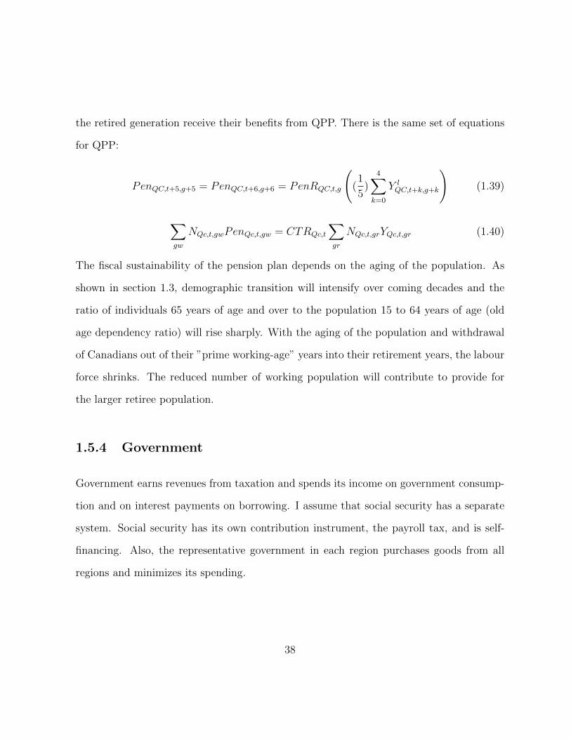
the retired generation receive their benefits from QPP. There is the same set of equations

for QPP:

PenQC,t+5,g+5 = PenQC,t+6,g+6 = PenRQC,t,g

((1

5)

4∑k=0

Y lQC,t+k,g+k

)(1.39)

∑gw

NQc,t,gwPenQc,t,gw = CTRQc,t

∑gr

NQc,t,grYQc,t,gr (1.40)

The fiscal sustainability of the pension plan depends on the aging of the population. As

shown in section 1.3, demographic transition will intensify over coming decades and the

ratio of individuals 65 years of age and over to the population 15 to 64 years of age (old

age dependency ratio) will rise sharply. With the aging of the population and withdrawal

of Canadians out of their ”prime working-age” years into their retirement years, the labour

force shrinks. The reduced number of working population will contribute to provide for

the larger retiree population.

1.5.4 Government

Government earns revenues from taxation and spends its income on government consump-

tion and on interest payments on borrowing. I assume that social security has a separate

system. Social security has its own contribution instrument, the payroll tax, and is self-

financing. Also, the representative government in each region purchases goods from all

regions and minimizes its spending.

38

The Government Budget Constraint

We assume government spending per capita remains constant over time; however, as the

population dynamics change the government issues bonds to keep the budget balanced.

The government targets a constant debt-to-GDP ratio. The government budget constraint

is as follow:

(1.41)PGi,tBi,t+1 − PGi,t−1Bi,t +

∑g

Ni,t,g[τLi,t(Y

Li,t,g) + τ ci,t(Ci,t,gPCi,t) + τKi,t(rei,tAi,t,g)]

= Gi,tPGi,t +

(rbi,t−1 +

PGi,t − PGi,t−1

PGi,t−1

)PGi,t−1Bi,t

where, Gi,t represents the government spending, PGi,t is composite government good price

index for region-i, re is expected rate of return on physical capital, Ni,t,g is population size

for generation g in region i and rb represents interest rate on government bonds. Different

taxes are assumed to be exogenous.

Government Optimization

The representative government in each region purchases goods from all regions and mini-

mizes its total spending. Government spending is a composite good of the three regional

final goods. The allocation of government spending across the regions is determined as

follow:

39

min Gi,tPGi,t =∑j

Pj,tgj,i,t (1.42)

subject to Gi,t =

∑j

αG,j,ig

σgi−1

σgi

j,i,t

σgi

σgi−1

(1.43)

where, gj,i,t represents public spending of government-i on goods from region-j. alphaG,j,i is

region-j share of region-i government consumption demand and σgi is the substitution elas-

ticities in government consumption. The first order conditions for government expenditure

minimization are derived by taking derivatives with respect to gk,i,t:

Pk,t = ν

∑j

αG,j,ig

σgj−1

σgj

j,i,t

σgj

σgj−1−1

αG,k,ig

σgj−1

σgg−1

k,i,t (1.44)

where, ν is the lagrangian multiplier. Multiplying both sides by gk,i,t:

gk,i,tPk,t = ν

∑j

αG,j,ig

σgj−1

σgj

j,i,t

σgj

σgj−1−1

αG,k,ig

σgj−1

σgg

k,i,t (1.45)

Taking the sum over all goods gives:

∑k

Gk,i,tPk,i,t = ν

∑j

αG,j,iG

σgj−1

σgj

j,i,t

σgj

σgj−1−1 ∑

k

αG,k,iG

σgj−1

σgg

k,i,t

(1.46)

40

Substituting equation (1.43) into the above equation yields the following form for the

Lagrangian multiplier:

Gi,t,gPGi,t = νGi,t,g ⇒ ν = PGi,t (1.47)

Replacing ν by its value into equation (1.45) gives the final government consumption

demand of region-i for good produced in region-k at period t, gk,i,t :

gk,i,tPk,t = PGi,tG1

σgii,t (αG,k,i)g

σgi−1

σgi

k,i,t (1.48)

gk,i,t = ασgiG,j,i

(PGi,t

Pk,t

)σgiGi,t (1.49)

Then using the constraint function, equation (1.43), and substituting gk,i,t, I derive the

composite government price index:

Gi,t =

[∑j

αG,j,i

(Gi,t(αG,j,i)

σgi PGσgii,tP

−σgij,i

)σgi −1

σgi

] σgi

σgi−1

(1.50)

PGi,t =

[∑j

(αG,j,i)σgi P

1−σgij,t

] 1

1−σgi

(1.51)

The composite government consumption price index is a non-linear weighted average of

regional prices.

1.5.5 Market Clearing Condition

Aggregate demand is composed of consumption demand, investment demands and govern-

ment consumption demand. Equation (1.52) shows the market equilibrium condition for

41

commodity market in region i. The total aggregate demand for each good is equal to total

output.

Qi,t = (∑g

Ni,t,gConi,t,g) + Ii,t +Gi,t +Xi,t −Mi,t (1.52)

Xi,t and Mi,t represent respectively region i’s export and import with other regions.

Also the market clearing condition for commodity market holds for Canada, in which the

GDP is equal to the sum of aggregate consumption, investment and net export.

The labour and capital are immobile across regions and input market clears for these

factors in each region. Equation (1.53) provides the equilibrium condition for labour mar-

ket. Capital market must be in equilibrium. This means that the total household saving

must be equal to stock of government bonds plus stock of capital,(equation (1.55)).

Li,t =∑g

Ni,t,gLSi,g (1.53)

Ki,t = Kstocki,t (1.54)∑i

∑g

Ni,t+1,gAi,t+1,g =∑i

PGi,tBi,t+1 +∑i

PIi,tKstocki,t+1 (1.55)

where, Kstocki,t is the exogenous supply of capital stock in region-i.

It is assumed that Canada is a closed economy. Obviously, other options were available.

First, I could assume a global model that incorporates the rest of the world regions. This

would be an ideal option but the model will become very large and hard to handle and

also very demanding in data in order to calibrate the model. Second, Canada could be a

small open economy that consequently it would be a price taker. Therefore it wouldn’t

be possible to study the impact of the demographic changes on domestic prices since they

42

would not alter. This would be hard to defend as all large economies of the world are now

aging. The third option, which is used in this chapter, is to assume a closed economy.

The advantage of making this assumption is that I can analyse the impact of demographic

changes on wage and interest rate. The disadvantage is that we implicitly assume that the

demographic changes in the Canadian economy are the same as the rest of the world. This

might not be far from the reality as demographic changes in Canada are similar to other

OECD (Organisation for Economic Co-operation and Development) countries.

43

1.6 Data and Calibration

The data for the calibration are obtained from Statistics Canada for the year 2007. We

use the symmetric Input-Output (I-O) tables for provinces and territories. The I-O tables

provide detailed statistics on all the transactions in an economy and involve production

activity and intermediate and final consumption of goods and services. We use the data

provided in the I-O tables jointly with other relevant data, such as government revenue and

expenditure 20, to create the Social Accounting Matrix (SAM) for Canada’s provinces. The

social Accounting Matrix provides a framework to analyse and build general equilibrium

models. Harberger [65] and Johansen [78] pioneered the application of SAM for providing a

data base to build an applied general equilibrium (Kehoe [81]). Since then, many research

studies have been developing general equilibrium (Scarf [120], Scarf [119], Shoven and

Whalley [121], Ballard et al. [13], Mercenier and Srinivasan [94], Dixon [41]).

The symmetric industry-by-industry I-O tables for Canada’s provinces represent the

most detailed accounting of the Canadian economy. They include data on labour and

capital value added, transactions among the 25 sectors, household spending, investment,

inter-provincial trade and international trade for each province. I use the I-O tables to

construct the SAM for each province and then I aggregate the provinces to create the

regional SAM 21. In this chapter, I assume each region has only one sector and therefore, I

aggregate across the 25 sectors. As an accounting principle, the total value of each column

20Government data are obtained from CANSIM tables, available at: http://www.statcan.gc.ca/

tables-tableaux/sum-som/l01/cst01/govt02a-eng.htm21We aggregate the SAM for Newfoundland and Labrador, New Brunswick, Nova Scotia and Prince

Edward Island to create the Atlantic region and aggregate Ontario, Manitoba, Saskatchewan, Alberta,British Columbia, Yukon, Nunavut and Northwest Territories to create the ROC and Quebec remains asa single province.

44

(expenditure) and its corresponding row (income) should be equivalent.

1.6.1 Demographic Structure

As mentioned in section 1.5, the population is divided into seven generations (i.e., 15-

24, 25-34, 35-44, 45-54, 55-64, 65-74, 75-84). The population data for the baseline year

are obtained from Statistics Canada, ”Population Projections for Canada, Provinces and

Territories” 22. Statistics Canada provides different population scenarios and we choose the

projection with medium growth in population; however, the population projection data for

Canadian provinces are only available until 2031. In order to have a longer horizon for the

model to allow it to converge to the steady state, I also use the population projections from

the United Nations 23. The United Nations Statistics Division provides national population

projection datasets by age groups until the year 2100.

The aging of the Canadian population based on United Nations data 24 is shown in

figure 1.6. The figure shows the proportion of children aged 14 years and less and persons

65 and over.

The share of older age groups continues to increase after 2031 with lower speed. As

demonstrated in Figures 1.6, the share of elderly population in Canada will increase from

13% in 2011 to 22% in 2100. The share of people aged 65 years and above continues to

be lower than those aged 14 years and less until 2022 and then it surpasses and remains

22The data are available at the following link: http://www5.statcan.gc.ca/bsolc/olc-cel/

olc-cel?catno=91-520-XWE&lang=eng23United Nations Population Censuses Datasets, available at: http://unstats.un.org/unsd/

demographic/products/dyb/dybcensusdata.htm24United Nations, World Population Prospects, 2012.

45

Figure 1.6: Proportion of Persons Aged 65 Years and Over and Children Aged 14 Yearsand Less in Canada, 1950-2100

Source: United Nations, World Population Prospects, 2012

above this group until the year 2100. While the senior population is continuously growing,

the proportion of children is decreasing. During the past two decades the share of children

aged 14 years and less has dropped significantly, and it was approximately 16% in 2011.

It continues to decreases with a lower pace until 2100.

As the United Nations population projections reveal, Canada will experience significant

demographic changes in the coming decade.

In order to obtain demographic variables such as survival rate and fertility rate for ex-

tended periods until the year 2100, I combine the data provided by the UN and Statistics

Canada. First, I calculate these rates for each cohort based on population projection data

available by Statistics Canada until the year 2031. Then, I use the UN population projec-

tion and calculate the cohorts survival rate for Canada from 2031 to 2100. Subsequently, I

obtain the trend in UN demographic variables and extrapolate the survival rates for each

46

age group from 2032 to 2100. This procedure will allow us to have demographic variables

for a longer horizon and improve the simulation results.

To simplify the model, I assume that demographic variables, fertility rate and survival

rate, are exogenous. Each generation has the following law of motions:

Ni,t,g+k =

Ni,t−1,g+k ∗ FRi,t−1 k = 0

Ni,t−1,g+k−1 ∗ SRi,t−1,g+k+1 k = 1, 2, 3, 4, 5, 6

where, FRi,t−1 represents the fertility rate, SRi,t−1,g+k+1 is the survival rate and Ni,g+k is

the population size for generation g + k in region i. The first law of motion indicates that

in region i at time t the number of the young generation (i.e, age group 15-24) is equal to

the size of the same cohort at time t-1 times the fertility rate at time t-1. The second law

of motion specifies the size of any generation (except the first generation) at time t equal

to the size of the same cohort at time t-1, times the survival rate of that generation at

time t-1. The survival rates are different for each generation at any period. The survival

rate for the last generation is equal to zero. Table 1.2 represents the projected old age

dependency ratio across the regions.

Table 1.1: Projected Old-age De-pendency Ratio

Region 2007 2020 2030

ROC 18.57 25.85 35.00Atlantic 20.56 33.25 47.18Quebec 20.85 30.23 40.81

Source: Statistic Canada, Population Projec-tion for Canada Provinces and Territories, Ta-ble 052-0005.

47

1.6.2 Calibration

I use SAM, first-order conditions, regions-specific exogenous parameters and market clear-

ing conditions to calibrate the model and obtain other parameters of the model and values

of the non-observed variables at the baseline year. The calibration is performed in three

steps to estimate the parameters of the model. In the first step, I employ the regional data

on output production, labour and capital demand and the first order conditions from the

production optimization to calibrate wage, rental rate of capital and the scaling parameter

(TFP) of production function.

The second step includes household optimization, market clearing conditions in goods

and assets and government budget constraints to derive consumption profile and gov-

ernment expenditure. Jointly, rate of time preferences, interest rate and intertemporal

elasticity of substitution determine the consumption profile. Also, government spending

adjusts to population dynamics. I assume that debt-to-GDP remains constant.

The third step calculates a matrix and estimates the distribution of wealth across

generations and regions. Individuals hold their wealth in the form of physical capital

and government bonds but the distribution of the wealth is unknown. Although assets

are perfectly substitutable and mobile across regions, it is important to know the initial

portfolio distribution in case of unanticipated shocks. Each individual’s wealth consists of

the local physical capital and bonds issued by local and other regional governments.

After the three steps, I use the calibration results to examine the model and verify

whether the model could replicate the observed data on baseline year. Then the calibration

results are used to simulate the impact of population dynamics on pension plan.

48

Table 1.2: Calibration Results

Region α A δ γ r

ROC 0.43 1.72 0.42 0.25 0.67Atlantic 0.48 1.45 0.21 0.15 0.47Quebec 0.39 1.64 0.34 0.17 0.59

Notes:α= share of physical capitalA= shift parameter in productionδ= depreciation rate over 10 year periodγ= inverse of intertemporal elasticity ofsubstitution over 10 year periodr= real rental rate of capital

1.7 Simulation

As mentioned in section 1.2, the main pillar of the income security system in Canada

consists of two pension plans. The residents of Quebec contribute to the Quebec Pension

Plan (QPP), while the rest of the provinces contribute to the Canada Pension Plan (CPP).

In order to investigate the impact of population aging on the pension plans I use the model

under steady state to calculate the contribution rate for each region, in three different

scenarios for pension programs and in two different years, 2007 and 2030.

For the first scenario, I assume that all the regions together have one single pension plan.

The working-age population from all three regions contributes to one pension system that

provides benefits for all the retiree population in all three regions. The pension equation

is equal to:

49

∑i

∑gw

Ni,t,gwPeni,t,gw = CTRt

∑i

∑gr

Ni,t,grYi,t,gr i ∈ (ROC,Atlantic, Qc) (1.56)

where, gw represents the working generation and gr is the retired generation. As the above

equation shows, in a PAYG system the working-age population contributes to the system

to provide for the benefits of the elderly. According to the above equation, the pension

plan has a single contribution rate that is the same for all regions.

For the second scenario, I take into consideration the current situation of the income

security system in Canada in which Quebec has its own pension plan (QPP) and Atlantic

and ROC regions are under CPP. Therefore, there are two pension equations, as follow:

∑gw

Ni,t,gwPeni,t,gw = CTRi,t

∑gr

Ni,t,grYi,t,gr i ∈ (ROC,Atlantic) (1.57)∑gw

NQc,t,gwPenQc,t,gw = CTRQc,t

∑gr

NQc,t,grYQc,t,gr (1.58)

According to equations (1.57) and (1.58), there exist two contributions rates. The

elderly in Quebec receive benefits from QPP while benefits to elderly in the ROC and

Atlantic are paid under the CPP.

For the third scenario, I assume each region has its own pension plan. Therefore, there

are three contribution rates and the pension equation is equal to:

∑gw

Ni,t,gwPeni,t,gw = CTRi,t

∑gr

Ni,t,grYi,t,gr i ∈ (ROC,Atlantic, Quebec) (1.59)

50

Table 1.3: Contribution Rates for Three Scenarios

The above three scenarios are calculated for the model and the results are reported

in Table 1.3. To do a comparative analysis among the three scenarios and across years,

I choose scenario one in 2007 as a benchmark and compare the results of scenarios two

and three with the benchmark. According to scenario one at baseline year 2007, the

contribution rate is 10 percent. If the economy switches to scenario two in which there are

two pension systems, one for Quebec and one for Atlantic and ROC, the contribution rate

for ROC and Atlantic drops by about 3 percent while the contribution rate for Quebec

increases by 10 percent in order to maintain its pension system. Quebec is better off under

a joint pension plan with other regions. The difference in the contribution rate is due to

the demographic structure of the working population.

As explained in section 1.3, the population aging is heterogenous across Canadian

regions. Under scenario one, the share of the retired population in the total population

is 12 percent; however, once the regions are separated and Quebec has its own pension

system, the share of the retired population in Quebec becomes 15 percent. This significant

51

increase in the share of the retiree population puts pressure on the provision of pension

benefits and leads to a rise in contribution rate.

If the economy chooses scenario three, the contribution rates for Atlantic region should

increase by 6 percent in order to maintain the pension system. The contribution rate in

ROC drops by 3 percent indicating that ROC is better off when it has its own pension

plan. The share of the working age population in ROC is significantly larger than the

share of the working age population in Atlantic and Quebec (by 6 times in Atlantic and 3

times in Quebec). Therefore, under a joint pension system, the larger and young working

population of ROC contribute to the provision of benefits of elderly in all three regions.

The retiree population is continuously growing in all regions by 2030. It increases by

60% in Quebec, 80% in the Atlantic and 46% in the ROC. These significant changes in the

structure of the population show that population aging is faster in Quebec and Atlantic

region.

The results for the three scenarios in year 2030 confirm that the aging of the population

imposes higher contribution rates to the pension plan. Comparing the results in 2030 with

scenario one in 2007 reveals that the contribution rate increases in all three scenarios and

the increase is higher in Quebec, if it keep its own pension system. In 2030, according to

scenario one, the contribution rate should increase by 66 percent from the benchmark, in

order to maintain the balance in the pension system. Under the scenario two the contribu-

tion rate should increase by 53 percent for ROC and Atlantic; however, the contribution

rate should increase more than 100 percent for Quebec in order to maintains its pension

system.

52

The main benefits of having a joint pension system are for the Atlantic. Under the

scenario three, the Atlantic region should increase its contribution rate by 100 percent, but

by joining to ROC under the scenario two, it pays lower contributions. Regions with faster

aging of the population benefit more from a joint pension system. The Atlantic region and

Quebec should double their contribution rates by 2030, if they choose to have a separate

pension plan. But, by joining to a joint pension system their contribution rates increase

by less.

A shrinking labour force has to provide for the growing retiree population. The share

of working age population declines for all regions from 2007 to 2030. It decreases by 9

percent in Quebec, 8 percent in the Atlantic and 4 percent in the ROC.

1.7.1 Implicit Transfers Across Regions

To calculate the implicit transfer of funds across regions and to get a good sense of the

amount of implicit transfers, I perform the following experiment, using the data on total

contributions to CPP and QPP for year 2013-2014 from Canada’s Pension Plan report 25. I

assume the economy’s pension system is scenario two. The total contributions paid to CPP

in 2013-2014 are $43.3 billion. This amount is contributed by the working age population

in both ROC and Atlantic region. I use the share of the working-age population in 2007

and estimate the share of each region in total contributions. The working-age population

in ROC is seven times larger than the working-age population in Atlantic. Therefore,

the amount of pension contribution paid by the ROC is seven times more than the total

25https://www.canada.ca/en/employment-social-development/programs/pensions/pension/

statistics/2015-quarterly-january-march.html

53

Table 1.4: Total Contribution for Three Scenarios, Using 2013-2014 Data, $Billions

contribution paid by Atlantic. Thus, the shares of ROC and Atlantic from the total

contributions of $43.2 billion are respectively, $37.7 and $5.4 billion. The results of this

experiment are reported in Table 1.4.

When the economy moves from scenario two to scenario three, in which each region

has its own independent plan, the working-age population in each region should pay for

the benefits of the retiree population in the respective region. The retiree population of

the Atlantic region is 1.6 percent larger than in the ROC, therefore the amount of benefits

paid to retirees of Atlantic is 1.6 percent larger than the amount paid to retirees in ROC.

Consequently, the total benefits paid to the retiree population are equal to $20.9 billion

and $22.2 billion in ROC and Atlantic, respectively.

As a result, under a PAYG pension system, the total contribution in the Atlantic region

should increase from $5.4 billion to $22.2 billion, while it declines from $37.7 to $20.9 billion

in the ROC. The difference between the two levels of contributions, which is equal to $16.8

billion, is the implicit transfer of funds (contributions) from the ROC to Atlantic region

when the economy chooses scenario two and ROC and Atlantic have a joint pension system.

54

The Atlantic region under scenario two pays $16.8 billion less in contributions, since it has

a smaller share of working population. Therefore, this amount is paid by the working

population of the ROC under a joint pension plan.

Quebec cannot benefit from the same type of implicit transfers if it chooses to have

a joint pension system with ROC and Atlantic. The contribution rate declines if Quebec

joins the other two regions, but since it has higher share of working population than the

Atlantic, it compensates for part of the benefits paid to retiree in Atlantic. In fact, if

Quebec chooses to join the other two regions to have a single plan (scenario one), it will

be worse off than having its own separate plan. This is because by having a shared plan

with other regions it will take away some of the pressure on the ROC in providing for the

Atlantic region. In other words, there is a small implicit transfer of funds from Quebec to

Atlantic. According to the pension plan report for 2013-2014, the total contribution for

the QPP is equal to $12.3 billion. Therefore, the total pension benefits in the economy

equal to $55.5 billion. Using the same justification as above, the amounts of pension

contributions in ROC and Quebec are, respectively, seven and three times larger than the

total contributions paid by Atlantic because the share of the working-age population is

larger, by the same ratio, in ROC and Quebec compared to Atlantic. Thus, under scenario

one, the shares of ROC, Atlantic and Quebec from the total contributions of $55.5 billion

are, respectively, $34.6, $5 and $15.8 billion. Comparing the results of scenarios one and

two shows the transfer of implicit funds from ROC and Quebec to Atlantic.

The share of the retiree population in Atlantic is larger than the retiree population

in ROC by 1.6 percent and the same share is 0.9 percent smaller in Quebec compared

to ROC. Therefore, if each region decides to have its own pension plan (scenario 3), the

55

amounts of benefits paid to the retiree population in ROC, Atlantic and Quebec are equal

to $20.94, $22.2 and $12.3 billion. By comparing scenario three with scenario two, the

implicit transfer of funds (contributions) from the ROC to Atlantic region is equal to $17

billion.

I repeat the same experiment for year 2030 to further explore the impact of aging and

the amount of implicit transfers. I use the same data on total contributions for year 2007.

The lower panel of Table 1.4 reports on the total contributions by region for year 2030. In

2030, the share of the working-age population in ROC is 6.6 times larger than in Atlantic,

therefore, under scenario two, the working age population in ROC will be paying for the

larger share of total contributions. Comparing the results of scenarios two and three shows

that the implicit funds transferred from ROC to Atlantic equal to $18 billion.

Moving from scenario two to scenario one in 2030, in which Quebec joins the other two

regions, benefits Atlantic region significantly, but it also reduces the pressure on the ROC

region by one percent. Also, in 2007 Quebec pays a higher amount of contributions than in

2030 under scenario one. In other words, for Quebec to have its own program is beneficial

in 2007 but that benefit is disappearing slowly and by 2030 the benefit is almost zero. The

big winner of the current system (scenario two) is obviously the Atlantic region, both in

2007 and in 2030.

56

1.8 Conclusion

This chapter provides, from a theoretical and quantitative point of view, a methodology

to investigate the impact of an aging population on the pension system from a regional

perspective. I developed, calibrated and simulated an OLG model to investigate the impact

of demographic changes on public pension and measure the transfer of implicit funds across

regions. Three scenarios are suggested for the pension system. The results show that as a

result of aging of the population, all regions are affected negatively if they choose to have

an independent pension system. Under a joint pension system most of the pressure of the

provision of the pension system is on the ROC, since it has the highest share of working

population. Atlantic region benefits the most from a joint pension plan, as the aging of

the population intensifies significantly in this region over the coming years.

ROC bears the brunt of a joint system. The pressure of providing pension benefits

for the elderly in Atlantic is mainly on the ROC, since it has a much larger working

population. If Quebec joins the pension plan with the other two regions, it takes away

some of the pressure on the ROC, by paying larger contributions. Therefore it is beneficial

for Quebec to have its own pension system; however, over time, as the share of working

population drops in Quebec, engaging in a joint pension system with other regions benefits

Quebec. This is because the larger share of working population in ROC is contributing to

the provision of pension benefits in Quebec. A joint pension system dramatically burdens

the future working population in ROC. Nonetheless, when reduction in GDP per capita

and cohort welfare are taken into account, all regions experience contractions in response

to aging of the population.

57

The model and the results contained in this chapter provide valuable and useful insights

on the consequences of a joint pension system in Canada. In particular, it shows that there

is an argument for Quebec to have its own pension program and not join the other regions

under a joint pension program and that the implicit transfers of resources from the west

part of Canada to the Atlantic provinces is substantial. The results of the chapter suggest

that it would be relevant in future research to investigate further the question by going

beyond the pay-as-you-go specification for the pension plan and incorporating the three

pillars of the Canada pension system.

58

1.9 Appendix for Chapter 1

1.9.1 List of variables

Subscript i indicates region:

Qi,t = region-i output

Pi,t= output price in region-i

Ki,t= physical capital

Kstocki,t= stock of capital in region-i

Li,t= effective unit of labour

ri,t= real rental rate of capital

Wi,t= wage for effective unit of labour

Ci,t,g= consumption demand of household of generation g at time t

xj, i, t, g= household-g of region-i’s consumption demand for region-j’s good

PCi,t= composite consumption price index

Ai,t,g= household-g stock of wealth at end of period t-1

Y li,t,g= labour income of household-g

LSi,g= labour supply by household-g

EPi,g= household-g age-dependent earning profile

Ni,t,gw= population size of working age cohorts

Ni,t,gr= population size of retired cohorts

Peni,t,gr=pension benefit to retired generation gr

Ii,t= investment in region-i

59

ij,i,t=region-j’s investment demand for region-i

PIi, t= composite investment good price

rei,t= expected rate of return on physical capital

rbi,t= rate of interest on region-i government bond issued at end of t-1

Gi,t= region-i public expenditure

Gj,i,t= government-i public expenditure on region-j good

PGi,t= composite government spending price index (price of bond issued by region-i gov-

ernment)

60

1.9.2 List of parameters

Subscript i indicates region:

Ai,t= total factor productivity

αi= share of physical capital in Cobb-Douglas function

ϕi= rate of time preferences

γi= inverse of the constant inter-temporal elasticity of substitution

τ ci = consumption tax rate

τ ki = tax rate on capital income

τ li= tax rate on labour income

τj,i,t= tariffs on goods

CTRi,t= contribution to the pension plan

PenRi,t,g= pension replacement rate

Peni,t,g= pension benefit

SRi,t,g= survival rate of cohort g at timet

δi= depreciation rate of capital

αC,j,i= region-j share of region-i consumption good demand

αI,j,i= region-j share of region-i investment good demand

αG,j,i= region-j share of region-i government good demand

σci= substitution elasticities in consumption goods

σIi = substitution elasticities in investment goods

σgi = substitution elasticities in government goods

ω= constant term in quadratic function of age

61

ξ= coefficient on age term in quadratic function of age

φ= coefficient on the quadratic term in age function

62

Chapter 2

Age Variable Rate of TimePreference in OLG-CGE Model

2.1 Introduction

Intertemporal choices require decision-making that involves trade-off between current and

future outcomes. Intertemporal choices and their outcomes are important for economists.

Economic models construct assumptions about preferences and sometimes these assump-

tions have led us to solutions that are general and abstract. Olson and Bailey [103] state

that ”without time preference, models of intertemporal choice do not yield predictions con-

sistent with observed behaviour”. The early studies on the importance of intertemporal

choices started in the early nineteen century with Scottish economist John Rae and Aus-

trian Economist Eugen von Bohm-Bawerk who examined the sociological and psychological

determinants of intertemporal choice. The perspective on intertemporal choices changed

in 1937 when Paul Samuelson proposed the discounted utility model as a ”descriptively

accurate” representation of individual behaviour. In his model, he assumes that all the

63

underlying motives for intertemporal choices are condensed into one single parameter, the

discount rate. Many studies began to employ innovative approaches to better understand

and highlight the origins and stability of the preference parameter over individuals life

cycles (Borghan et al. [25], Posner [107], Trostel and Tyler [125]).

Over the past three decades, due to the anomalies and inconsistencies in the discounted

utility model, a series of theoretical and empirical studies attempted to explain and measure

discount rate. The theoretical studies attempted to make more realistic assumptions such

as relaxing the assumption of constant discounting, or incorporating more considerations

into utility function such as the ”utility from anticipation”, ”habit formation function”

and ”reference point model” (Laibson [89], Strotz [122]). The empirical studies derive

estimates of discount rate by observing ”real-world” behaviour (Rutherman et al. [114],

Kirby [83], Burks et al. [33]). There is a striking variation in the estimated discount rate

among empirical studies, which is mostly due to the elicitation procedure.

In this chapter, I review the existing theoretical and empirical research on intertemporal

choice. Recent empirical studies have demonstrated that the age profile of consumption

is bell shaped (National Transfer Account, United Nations 20131). This allows for a new

calibration procedure in which the rate of time preference varies by age. The advantage

of the new procedure is that it respects consumption behaviour observed in data. The

consumption profile derived from NTA allows the development of a new approach that

measures the rate of time preference more accurately. Contrary to the mainstream studies

in the area of intertemporal optimization that assume a constant rate of time preference

over individuals’ life cycles, I describe a new approach in which the rate of time preference

1http://www.ntaccounts.org/web/nta/show/Methodology

64

evolves by age. I construct an OLG model and assume that people are not characterized

by a constant rate of time preference and allow the rate of time preference to vary with

age. Age-variable rate of time preference would permit us to capture many other elements

that affect the life cycle profile of consumption observed in the data. Better-calibrated

life cycle profiles should improve simulation results. I also derive the asset holding by

age and compare it at the individual level with the total asset holding for the economy.

Furthermore, I investigate the sensitivity of the calibrated rate of time preference to the

other parameters of the model.

The rest of the chapter is organized as follows. In section 2.2, I review the various studies

that have attempted to explain the intertemporal choice and discounting behaviour and

highlight the assumptions underlying those studies. Section 2.3 describes the OLG model

developed to measure the rate of time preference. Section 2.4 describes the calibration

process and sections 2.5 and 2.6 explain two calibration approaches. Section 2.7 reports

the calibration results and section 2.8 concludes.

65

2.2 Review of Relevant Literature

In this section, I review the existing literature and highlight the striking variations across

studies that attempt to explain and measure the rate of time preference. I stress out

the importance of non-economic factors affecting individual time preferences and therefore

discount rate.

Investigating the determinants of intertemporal choices goes back to the early nine-

teenth century. Rae [108] invented the topic of intertemporal choice and recognized the

non-economic factors, sociological and psychological, that determine individuals’ intertem-

poral choices and therefore the level of saving and investment.

Rae [108] strives to explain why wealth differs among nations. Earlier, Adam Smith

argues that national wealth is determined by labour allocation toward production, ;how-

ever, Rae [108] believes that this explanation is incomplete and the missing element is ”the

effective desire of accumulation”. In his view, a psychological factor that is different among

countries determines individuals’ preferences toward saving and investment. He lists two

main elements that determines the accumulation: bequest motive and ”propensity to ex-

ercise self-restraint”2. For the first time, Rae [108] defined intertemporal choice and its

underlying motives for time preferences. He develops two views. In the first one, he claims

that individuals care about current consumption and postpone consumption only if they

anticipate higher utility in the future. The second view treats present and future outcomes

equally. In other words, individuals have no intrinsic preferences toward either present or

future consumption. Based on these two views, ”intertemporal choice behaviour” shapes

2” The extent of intellectual powers and prudence in the minds of the members of society”.

66

differently, but in both views people’s mental ability in imagining future situations affects

their intertemporal choice.

The next major figure in development of intertemporal choices is Eugen von Bohm-

Bawerk [23]. He added a new factor to the list proposed by Rae, arguing that people’s

intertemporal choices are affected by ”systematic tendency to underestimate future wants”.

He begins modeling the intertemporal choice by allocating one’s resources to different points

in time. Bohm-Bawerk concurs with Rae that humans’ decisions are heavily dependent on

psychological traits. The early theoretical framework developed by these authors became

the dominant theoretical framework for studying intertemporal choice.

A decade later Irving Fisher formalized Bohm-Bawerk’s approach and developed the

intertemporal consumption decision on a two-good indifference curve with consumption

in the current year and following year. Fisher [52], as for Bohm-Bawerk, differentiates

between ”objective factors” and ”personal factors” that affect individuals’ decisions over

time. In their views, time preference is an amalgamation of diverse intertemporal motives

that change over lifetime. In Fisher’s depiction, consumption depends on two factors: time

preferences and diminishing marginal utility. Fisher, like Rae and Bohm-Bawerk, considers

psychological factors in the determination of time preferences.

In 1937, Paul Samuelson introduced the discounted utility model. He condenses all the

analysis of time preferences mentioned by his predecessor into one single factor: discount

rate. Samuelson [117] developed a ”generalized” model of intertemporal choices with mul-

tiple time periods. An underlying assumption for Rae [108], Bohm-Bawerk [23], Fisher

[52] and Samuelson [117] is the constant discounting, which means that individuals have a

67

single, constant discount rate over life cycle.

Over the past four decades a body of research, both theoretical and empirical, has been

developed on intertemporal choices and these studies suggest that the discount rate is not

necessarily constant over time.

Many studies attempted to improve the theoretical model developed by Samuelson.

These studies formulate more realistic assumptions by incorporating more considerations

into utility function, such as relaxing the assumption of constant discounting (Thaler

[124], Chapman and Elstein [35], MacKeigan et al. [92], O’Donoghue and Rabin [101],

ODonoghue and Rabin [102]), including ”habit formation function”3 (Pollak [106], Becker

and Murphy [17]) and using ”reference point concept” 4 (Tversky and Kahneman [126],

Lowenstein and Prelec [91], Laibson [89], Stortz [122]).

The empirical studies derive estimates of discount rate by observing ”real-world” be-

haviour (Rutherman et al. [114], Kirby [83], Burks et al. [33]). There is a striking variation

in the estimated discount rate among empirical studies, which is mostly due to the elic-

itation procedure. The estimated discount rates range from -6 to infinity (Frederick et

al.[55]).

In the following sections I review the literature on time preferences and divide the

studies into three main categories: natural selection, psychological traits and experimental

studies.

3Habit formation means that individuals’ current preferences depend on their past consumption pat-terns.

4The reference point concept demonstrates that when people choose between immediate and delayedconsumption, the reference point used to evaluate alternatives can significantly influence choice. Prefer-ences formation may differ using reference point concept.

68

2.2.1 Time Preferences and Natural Selection

Some of the studies on theory of time preferences propose that preferences originated from

”natural selection”. In other words, individuals’ preferences are affected by their biological

characteristics such as size, shape and pattern of fertility. These models link discount

rate with age, because fertility capacity varies with age. Reproduction requires successful

propagation of one’s genes, which necessitates spending resources. These studies claim

that the time preferences are affected by theory of the evolutionary genetics5. They argue

that ”if genes affect preferences, then an evolutionary model may succeed in predicting

them” (Becker [16], Hirshleifer [69], Rubin and Paul [112], Ursprung [127]).

Roger [111] discusses the hypothesis that human time preferences are in evolutionary

equilibrium 6. This hypothesis defines ”Marginal Rate of Substitution (MRS) in fitness

as the marginal rate at which two goods can be substituted without changing Darwinian

fitness”7. By assuming that in evolutionary equilibrium the MRS in fitness must equal MRS

of preferences, Roger [111] estimates the evolutionary discount function. His model shows

that younger adults ”should discount at a higher rate than their elders” because ”young

adults seem to live as if there were no tomorrow”. Roger [111] identifies three factors

that encourage individuals to choose immediate over delayed benefits: ”expectation of

rising consumption”, ”declining reproductive value” and the possibility of future benefits

5Human evolutionary genetics studies how one human genome differs from another human genome,the evolutionary past that gave rise to it and its current effects.

6”An equilibrium that no mutation changing time preferences could be favoured by natural selection.”7” In models with discrete generations, Darwinian fitness is the conditionally expected number of an

individual’s offspring, given its genotype. In models with overlapping generations, fitness is measured by”Malthusian parameter”, which measures the asymptotic rate of exponential increase in the numbers ofone’s descendants.”

69

to be received by descendants rather than the individual himself. For the second factor,

reproduction declines because fertility declines with age. This element underlies the age

effect in his model. As individuals age the reproductive value declines and encourages

individuals to choose present benefits rather than delayed benefits.

Posner [107] asserts that discounting exists because individuals have ”multiple selves”,

that is ”people are weighting their present consumption far more heavily than their future

consumption...[because] the present self and the future self are, in some meaningful sense,

separate persons”. This argument favours separable utility functions (Koszegi [85]). Becker

and Mulligan [18] contend that the reason for discounting is ”rational defective recognition

of future utilities”. They show that elements such as wealth, addiction, mortality and

uncertainty affect the ”degree of time preferences” across cohorts. For example, wealth

can improve patience and the ”patience endowment” can be transferred from one cohort

to another.

Trostel and Taylor [125] argue that individuals do not have an ”intrinsic preference” for

present consumption but with aging they increase discounting (or have a lower rate of time

preference) because their expected utility falls as their physical and mental health declines.

The two authors construct a new theory of time preferences with this hypothesis that ”the

instantaneous utility function is expected to vary with age, just as people’s physical and

mental abilities vary with age”. In other words, the capacity to enjoy consumption is

expected to rise while young and therefore discount rate may be negative. Trostel and

Taylor [125] use household consumption data from the Panel Study of Income Dynamics

(PSID)8 and test their theory by estimating discount rate as a function of age, income,

8PSID contains 14 years of consumption data on income and demographic data, from 1974 to 1987.

70

education and race. Their estimation results confirm their theory on increasing discount

rate due to the decline in physical and mental health.

Robson and Samuelson [109] also assume that people’s preferences are affected by bi-

ological evolution. They show theoretically that individuals discount future reproduction,

because an ”intervening death” may prevent individuals from realizing future outcomes.

They derive an equation for discount rate, which is a product of population growth rate

and death rate. When there is an idiosyncratic uncertainty, the discount rate is equal

to the product of population growth rate and death rate; however when there is aggre-

gate uncertainty 9 the discount rate surpasses the product of population growth rate and

death rate. Aggregate uncertainty breaks the link between discounting and the sum of

the growth and death rates. They show that aggregate uncertainty lowers the growth rate

”below that arising with comparable idiosyncratic uncertainty”. Aggregate uncertainty

slows down population growth but it does not distort the trade-off between current and

future outcomes and hence the discount rate. Therefore, the product of the growth rate

and the death rate falls behind discounting.

Robson and Szentes [110] use Rogers’ [111] biological approach and reexamine the func-

tional form for the discount rate. They show that the functional form of the utility function

does not produce an equilibrium evolutionary behaviour. Roger [111] assumes that utility

function of an individual is derived from ”reproductive value” and all offspring are identical;

however Robson and Szentes [110] allow for different types of offspring, based on their level

of transfers that vary with age. They show that offspring with larger (intergenerational)

9Aggregate uncertainty, such as fluctuations in the weather, epidemics and failures of food sources areall bound to have a common effect on death rates.

71

transfers have higher reproductive value.

Fisher [51] argues that future rewards are discounted because ”an intervening death may

prevent us from realizing such rewards”. The possibility of death plays an important role

in individuals’ discounting behaviour. When there is a risk affecting individuals’ survival

rates, the constant discounting may not hold. Uncertainty affects intertemporal choice and

its effect differs across ages. In the presence of uncertainty, discount rate varies with age

(Robson and Szentes [110]).

Curry [37] supports the ”evolution of time preferences under natural selection” by

assuming that individuals care about the number of offspring they produce. Individuals

make decisions under uncertainty and choose from sets of risky alternatives (lotteries).

These lotteries are choices over commodities that may involve uncertainty. Commodity

choices at present time are transformed into expected surviving offspring in the next period.

To choose the optimal selection of lotteries, Curry [37] uses the Robson [109] evolution

criterion that gives the preferences to lotteries that maximize reproductive value. Curry

[37] shows that a lottery should be selected only if it maximizes ”expected number of

offspring relative to the average number of offspring in the population”. When all agents are

maximizing reproductive value, a game is constructed based on the choice among lotteries

(expected number of offspring). By allowing for this kind of preference, the reproductive

value is maximized and a unique Nash equilibrium is reached.

Blackburn and Cipriani [20] show that an increase in the probability of survival increases

the future returns on human capital accumulation and therefore causes the opportunity

cost of current work and reproduction to increase. Individuals increase their human capital

72

in exchange for a smaller number of children. The paper endogenises the survival rate by

allowing it to change as a function of the economy. They develop an overlapping generation

model with three generations and endogenous survival rate. Individuals choose between

consumption and number of children. They show that time preferences are affected by

changes in survival rate. When probability of survival increases, individuals expect to live

longer and opt for more education versus child bearing.

Rutstrom et al. [115] show that reasonable estimates of discount rate depend on joint

estimation of risk and time preferences rather than separate estimation. In their experiment

to jointly elicit time preference and risk, they use a utility function for income and con-

sumption, and present individuals with one task that indicates ”risk attitude” and another

task that indicates ”discount rate”. They show that ”joint elicitation of risk and discount

rate results in significantly lower discount rates than separate elicitation of discount rate”.

They performed a field experiment10 to collect data on a Danish adult population.

2.2.2 Personality Traits and Time Preferences

There is a huge literature in psychology on the importance of personality traits on economic

outcomes, such as job performance, health and academic achievement (Barrick and Mount

[14]; Chamorro-Premuzic and Furnham [34]; Hogan and Holland [70]; Hampson et al.

[64]). Individuals’ personality traits affect the choices they make at any age. These traits

are not stable over life cycle and consequently, individuals’ preferences vary over time.

Heckman and Honore [68] discuss the relevance and importance of personality traits in

10Rutstrom et al. [115], Chapter 4, page 18.

73

economics and show that learning ability affects consumption, labour supply and earning

profiles. They incorporate the measurement of learning ability in a life cycle model and

show that ”more able people are more likely to attend more years of school” and individuals

with higher levels of education have lower discount rates. Rubinstein and Heckman [113]

use the data from the General Education Development11 (GED) program to show the

”quantitative importance” of personality traits. They show that GED recipients have the

same cognitive ability as high school graduates but they differ in personality traits. GED

recipients perform poorly in the labour market compared to high school graduates.

Most studies in the field of psychology are dependent on questionnaires that capture

personality traits. Many economic studies strive to measure standard economic preference

parameters such as time preferences. Economic studies are now beginning to incorporate

psychological measurements of personality traits into economic models and filling the gap

between personality psychology and conventional economic preferences. Personality traits

affect individuals’ choices and basically their time preferences over the life cycle. In other

words, psychological characters appear as constraints into individuals’ optimization.

Personality traits are defined as ”patterns of thought, feelings and behaviour” (Borghans

et al. [25]). One of the most prominent personality trait measurements is the ”Big Five”12,

which economists have begun to use.

Considering the impact of personality traits on life outcomes, it is important to under-

stand how much and to what extent they can change over time and how environments and

investments affect development of personality traits. Environments and investments can

11An exam-certified alternative high school degree.12Conscientiousness, openness, emotional stability, extraversion, agreeableness.

74

have an immediate or short-term impact as well as long-term impact on behaviour. For

example, individuals will most probably invest more efforts if they are compensated to do

so and will be ”more sociable” if there are incentives to do so (Borghans et al. [25]). Con-

sequently, the individual’s behaviour will vary in different settings. Therefore, taking the

”malleability” of personality traits into analysis is essential because ”certain personality

traits are more susceptible to change over individuals’ life cycles” (Borghans et al. [25]).

Studies in psychology use various methods13 such as Mean-level change to capture and

measure the ”malleability” of personality and its impact on economic performance. Mean-

level change considers ”changes over time in absolute levels of a trait and is measured by

changes in personality scores over time.”14

Many studies in the field of psychology and economics estimate time preferences using

”observational data” (Heckman and Honore [68]; Borghans and Golsteyn [26]; Hausman

[67]; Ruderman et al. [114]); however, this type of study suffers from imperfect information

and consequently the interpretation of discount rate estimated this way will be complicated.

For example, Borghans and Golsteyn [26] explore the relationship between body mass index

(BMI) and proxies for discount rates; however, the relationship is not only dependent on

the choice of the proxy but also on the other parameters that determine the intertemporal

decisions. These empirical studies are discussed in section 2.3.

13Some other methods to measure changes in personality traits are: Rank order change, normativechange and non formative change. Rank order change refers to changes in the ordinal ranking of a trait ina population and is measured by test-retest rank correlations. Normative changes are ”changes that aretypical of average individuals in a given population, and caused either by biological programming or bypredictable changes in social roles”. Non normative change ”encompasses both intentional change, causedby deliberate, self-directed efforts, deliberately chosen changes in social roles and atypical life events”.

14Psychologists believe that it’s impossible to see dramatic change in mean-level change in personalityafter adulthood.

75

To avoid issues concerning observational data, some other studies use an experimental

approach to estimate discount rates. They use a series of monetary rewards for people

choices. Discount rate changes with the size of the reward (Green et al. [60], Kirby [83])

and with type of the reward (Chapman et al. [36], Bonato and Bolan [24]); however,

these monetary choices are usually hypothetical and therefore individuals may choose not

to maintain their preferences when faced with real life situations (Fuch [56], Green and

Myerson [60], Kirby and Marakovic [84]).

Discount rate estimates are affected by the context of study and they may not suc-

cessfully demonstrate separable economic preferences. Kahneman et al. [79] argue that

individuals’ choice in the valuation of environmental public goods does not comply with

economic preferences. They introduce the concept of ”attitude” that determines the size

and the strength of an individual’s stated willingness to pay for public goods. By including

”personality attributes” into the utility function and outlining ”dynamic constraints con-

nected with skill and trait formation”, utility optimization becomes consistent with more

”general preference specifications” (Phelps and Pollak [105], Ainslie [3], Laibson [89]).

Frederick et al. [55] propose a tri-dimensional rate of time preference, consisting of

three motives: ”Impulsivity” 15, ”compulsivity” 16 and ”inhibition” 17, and claim that

these dimensions can be measured accurately. They do not argue a precise link between

rate of time preference and these personality traits and state that more analysis is required

to clearly estimate a rate of time preference that is a composite of these dimensions.

15Tendency to act spontaneously and without planning.16Tendency to stick with plans.17Ability to override automatic responses to urgencies or emotions.

76

Borghans et al. [27] use a variety of personality trait measurements to predict social and

economic outcomes and show to what degree the traits are stable over the life cycle. They

create a framework for choice model that imposes psychological variables as a constraint

and preference parameter is derived as a consequence of these constraints. They conclude

that certain economic concepts require modification in order to fully capture the impact

of psychological traits into the choice model.

Borghans et al. [25] show the importance of personality traits by comparing the impact

of Big Five personality traits and IQ on time preferences and economic performances such as

job performance, college grades and years of education. They show that conscientiousness

is the best personality trait in predicting college grades and years of education. Chamorro-

Premuzic and Furnham [34] investigate other aspect of conscientiousness such as self-control

and perseverance on individuals’ success in school and in life. Nyhus [100] shows that

emotional stability leads to higher wages. Salgado [116] and Hogan and Holland [70] show

the importance of emotional stability in predicting job performance across professions.

2.2.3 Experimental Studies

There is a group of studies that use observational data to observe and measure time pref-

erence and display its variability. Although the scope of these studies is limited to specific

subject matter, they provide insight on choice preferences (Hausman [67], Ruderman et al.

[114], Gately [57], Borghans et al. [27]). The estimated time preferences by various stud-

ies, depending on the characteristics of the population, psychological state of individuals

77

and particular procedure or situation, range from -6 to infinity (Frederick et al [55])18. A

positive rate of time preference means that individuals are willing to sacrifice one unit of

consumption today for more than one unit of consumption later. A negative rate of time

preference would require substantial reductions in present consumption in favour of the

future.

Borghans et al. [27] investigate individuals’ emotional stability and conscientiousness

in performing IQ tests. By providing financial incentives, they measure to what extent

people are responsive to these incentives. They show that individuals spend more time in

answering questions if they are offered financial reward. Multiple financial incentives were

offered to the participants and the amount of time spent on the test was measured, along

with their performance. The discount rate varies between 0 and 0.6 and its mean is 0.247.

They chose 128 students from Maastricht University for the experiment and concluded that

people with motivation and self-discipline are more successful in the test and have lower

discount rate.

Hausman [67] studies individuals’ behaviour in the market for durable goods. He in-

vestigates the trade-off between ”capital costs” and ”operation cost” in the market for

energy efficient air conditioners and measures discount rate in purchasing air conditioners.

He uses household data from a Midwest Research Institute (MRI, 1978) survey for energy

consumption and electricity appliances. The MRI survey includes a random sample of

1985 households in sixteen cities across United States. This survey also collects socioeco-

nomic data for each household in the sample. Individuals consider ”initial capital cost”

and ”operating cost” when making decisions toward purchasing energy efficient appliances.

18Fredrick et al. [55] survey methods for measuring discount rate.

78

Individuals trade off ”capital costs” and expected ”operating cost” and therefore the rate

of substitution among energy appliances depends on the above two factors.

In other words, when the ”capital cost” is high, individuals opt for purchasing energy

efficient appliances only if ”operating cost” is low. His estimation results show individuals

use a discount rate of 20 percent in making the trade-off. He comments that a high level

of discount rate can be reduced if the choice of other energy-using appliances is added to

the analysis. If consumers have more options available the estimated discount rate might

be lower.

Ruderman et al. [114] analyse the market for energy appliances and estimate the

discount rate. They use historical data from surveys of appliance manufactures. The

data consist of energy cost, purchase price and efficiency factors and are captured by

the U.S Department of Energy for 1972-80. They measure the aggregate discount rate

for eight products by assuming that individuals minimize the life cycle cost over these

products. Their results show that higher discount rate is associated with lower sensitivity

between energy consumption and appliance efficiency. Also, discount rates for various

energy appliances show the same trends. They justify high discount rates by unavailability

of full information for consumers.

Hardisty et al. [66] extract time preferences for financial gains and losses for delays

up to 50 years. They employed various methods such as matching, fixed-sequence choice

iteration and a dynamic ”staircase” choice method. They recruited five hundred sixteen

participants from the virtual lab participant pool of the Center for Decision Sciences at

79

Columbia University and randomly assigned an experiment 19. Unlike other studies that

use short-range delays of gains and losses, Hardisty et al. [66] use long timescale (50 years),

to model ”real-world” intertemporal choices. For all methods used, they find that gains

are being discounted more than losses, which means that participants’ wish to have gains

immediately is stronger than their wish to postpone losses.

Anderoni et al.[4] use two methods, convex time budgets (CTB)20 and double mul-

tiple price lists (DMPL), 21 to elicit the discount rate. They show that the discounting

behaviour is different with and without accounting for curvature of utility function. Esti-

mated discount rate is lower for linear utility function. They evaluate the predictive power

of the estimated parameter and show that both methods make predictions close to average

behaviour.

Burks et al. [33] calculate measures of time preference and test the measures to evaluate

how well these measures predict important health outcomes such as smoking and Body

Mass Index (BMI), credit scores and subsequent job related outcomes. They use a large

(1069 participants) sample of ”non student subjects” (trainee truckers) who participated

in an extensive set of economic field experiments between December 2005 and August 2006

and gather data on preference and outcome. Their results show that all measures of time

preferences predict individual behaviour to some extent.

19Hardisty et al. [66], page 239.20”Given a set of functional form assumptions about discounting and curvature of the utility function,

preference parameters are estimated at either the group or individual level.”21”This method compares safe and risky gambles with different payoffs and different odds, including

some gambles that payout with certainty. The response to risky choices identifies attitude towards risk bythe point at which individuals switch from a safe payout to a risky gamble. This information identifies thedegree of utility function curvature”.

80

This section reviewed the existing literature in estimating and measuring time pref-

erence. Individual differences in personality and cognition shape the constraints of indi-

viduals and therefore their choices over the life cycle. Many studies argue that constant

time preference for choice behaviour is an unrealistic assumption. Individuals’ preferences

change through the life cycle due to various elements such as age, health, personality traits,

etc. If these elements are considered in shaping the individuals’ preferences, the rate of

time preference will not be constant over life cycle. This chapter contributes to this litera-

ture by assuming that the rate of time preference is not constant and is dependent on age.

In the next section we describe an OLG model with age dependent rate of time preference.

81

2.3 Model Description

The model is a modified version of Auerbach and Kotlikoff [7] and Auerbach et al. [8]. It

is an OLG model with three sectors, 21 generations and exogenous labour supply. Two

of the sectors are public goods (education and health) and the third is the unique private

good sector. In this section, I give an overview of the model. In the next section, I discuss

in detail the calibration challenge of such a model.

2.3.1 Firm Behaviour

The representative firm maximizes its profits by employing labour and capital. It is as-

sumed that capital is homogeneous and depreciating. Labour supply differs in its efficiency

because individuals of different ages provide different amounts of labour input. The pro-

duction function is assumed to be of the Cobb-Douglas form with constant return to scale.

Perfectly competitive firms maximize profits. The demand for factors of production is

derived accordingly.

2.3.2 Household Behaviour

There are 21 overlapping generations 22 that live side by side. Each generation lives 21

periods of 5 years. Individuals in an age-cohort are identical and they have identical tastes.

An individual is born at the age zero, enters the labour market at age 20, retires at age

22The 21 age cohorts are: 0-4, 5-9, 10-14, 15-19, 20-24, 25-29, 30-34, 35-39, 40-44, 45-49, 50-54, 55-59,60-65, 65-69, 70-74, 75-79, 80-84, 85-89, 90-94, 95-99 and 100+.

82

65 and dies at age 100. The first four generations (children) do not contribute to the

economy and they do not have active roles in the model. Individuals are assumed to be

forward-looking with perfect foresight. Individuals make lifetime decisions on consumption

based on life cycle behaviour and they have bequest motives. The oldest generation leaves

a bequest for the first working generation 23. Also, as households encounter uncertain life-

times, they might leave ”unintentional bequests” 24 (Barro and Friedman [15]). Assuming

a ”perfect annuity market”, the unintentional bequests are evenly distributed across the

active generations 25. The household preferences are represented by a Constant Elasticity

of Substitution (CES) function with current and future consumption. Households max-

imize the inter-temporal utility function with respect to the budget constraint to derive

the consumption demand. The rate of time preference denotes the degree to which the

households prefer current consumption over future consumption during their lifetimes.

Future utilities are discounted by an exogenous survival rate. This form of utility

function imposes some constraints on preferences. At any point in time the individuals’

decisions depend only on current and future consumption. Past levels of consumption

affect households’ current wealth.

23This assumption is made in order to ensure the model solves. In calibrating the Euler Equation,(equation (2.17)), due to the ratio of C(g+1)/(C(g), the number of equations is one less than the numberof variables. By assuming that the oldest generation leaves a bequest for the first working generation, oneequation is added to the model and guarantees feasibility of the solution.

24Unintentional bequest occurs when the date of death differs from what the individual might forecast.25The unintentional bequest approach was first developed by Yaari [130], for a continuous time model.

Application of this theory to the overlapping generation model was implemented by Borsch-Supan et al.[28].

83

Budget Constraint

In each period, the household earns income from labour and capital and decides how

much to spend on consumption. The remainder is saved and added to its lifetime stock

of assets. The present value of lifetime consumption should be equal to the present value

of lifetime earnings. Individuals contribute to the pension plan when young and receive

pension benefits when retired. Individuals have no labour income and stop accumulating

assets when retired.

2.3.3 Pension

I assume that the pension plan is a PAYG (pay as you go) system. Therefore, the total

pension benefits should be equal to the total contributions. Contribution rates of the

pension program are dependent on the age distribution of the population. Retirees receive

pension benefits that are proportional to their lifetime earnings.

2.3.4 Government

Government earns revenues from taxation and spends its income on government consump-

tion, education, health and interest payments on borrowing. The government targets a

constant debt-to-GDP ratio. We assume government consumption per capita remains

constant over time; however, public spending on education and health is sensitive to the

age structure of the population. Consequently, as the population dynamics change the

government will adjust the income tax to keep the budget balanced.

84

2.3.5 Market Clearing Condition

The model is a closed economy and all markets are competitive. Labour supply equals to

labour demands. With population aging, labour supply becomes scarce hence wage rate will

rise. On the contrary, capital demand will decline for the same reason and capital return

will drop. Aggregate demand is composed of consumption demand, investment demand

and government consumption demand. The market equilibrium condition for commodity

market ensures that the total aggregate demand is equal to total output.

85

2.4 Calibration

2.4.1 Data

The model is calibrated using United Kingdom (UK)data for the year 201026. The popu-

lation projection data are from the Office for National Statistics (ONS)27 and are used to

derive fertility rate, survival rate and migration rate. The formula is provided in section

4.2. Data on GDP, public revenue and expenditure are extracted from ONS. Data on

pension are taken from the Government Actuarial Department (GAD)28. Labour income

tax, consumption tax and capital tax are calculated using the government revenue data 29.

Labour force data are obtained from the Labour Force Survey in ONS. The data obtained

are used to derive the Social Accounting Matrix (SAM). Table 2.1 provides the SAM for

the base year 2010.

SAM is a particular representation of the macro and intermediate economic accounts of

a socio-economic system, that captures the transactions and transfers between all economic

agents. As we can see in Table 2.1, the value added of production is captured in rows 5 and 6

(capital, labour, with the sum of them constituting GDP). Final consumption expenditure

by households is shown in column 7, government spending in columns 8-10 and investment

in column 10.

26The UK data are used in this chapter due to the availability of long term population projection datafor all age groups. Canadian population projection data per province is merely available until 2031. Thislimitation hinders the calibration of a large model such as the one deployed in this chapter.

27http://www.ons.gov.uk/peoplepopulationandcommunity/populationandmigration/

populationprojections/bulletins/nationalpopulationprojections/2011-10-2628https://www.gov.uk/government/uploads/system/uploads/attachment_data/file/220568/

pesa_2010_complete.pdf29http://budgetresponsibility.org.uk/download/public-finances-databank

86

Table 2.1: Social Accounting Matrix, United Kingdom, £mil, 2010

In our new calibration procedure, I also use life cycle data on labour income and

consumption. These data will be presented in the following sections.

2.4.2 Demographic Structure

The population data for the baseline year (2010) is obtained from the Office of National

Statistics (ONS), which provides projections up to the year 2100. In order to obtain

demographic variables such as survival rate, migration rate and fertility rate for extended

periods until year 2100, we calculate these rates for each cohort using population projection

data.

To simplify the model, I assume that demographic variables, fertility rate, migration

87

rate and survival rate, are exogenous. Each generation has the following law of motions:

Nt,g+k =

Nt−1,g+k+5 ∗ frt−1 k = 0

Nt−1,g+k−1 ∗ (srt−1,g+k+1 +mrt−1,g+k+1) k = 1, 2, ...19,

where, N represents population, frt−1 the fertility rate, srt−1,g+k+1 is the survival rate

and mrt−1 represents migration rate. The first law of motion indicates that the number of

children (i.e., age group 0-4) at time t is equal to the size of the first adult generation times

the fertility rate at time t-1. The second law of motion specifies the size of any generation

(except the first generation) at time, t, equal to the size of the same cohort at time t-1,

times the sum of survival rate and net migration rate of that generation at time t-1. The

survival rates are different for each generation in any period. The survival rate for the last

generation is equal to zero.

2.4.3 Calibration Procedure

In this section I review the fundamental aspects of the calibration procedure that underlies

most overlapping generations computable general equilibrium (OLG-CGE) models and in-

troduce a new approach for calibrating the model described in section 3. The calibration

procedure is sequential and there are two sets of parameters: predetermined and free pa-

rameters. Predetermined parameters are estimates from other studies and are regarded as

exogenous in this model.

The model described in section 2.3 is solved to derive the first order conditions. Data

obtained from SAM, first-order conditions, exogenous parameters and market clearing

88

conditions are used to obtain the other parameters of the model and values of the non-

observed variables at the baseline year. The calibration procedure allows one to determine

the scaling parameter of production, the depreciation rate, the age-specific consumption

and the rate of time preference, assuming that all markets are in steady state equilibrium.

Production

I calibrate the supply side of the economy by using data from SAM. Deploying the data

on labour demand, capital demand and total output from SAM and assuming a Cobb-

Douglas production function, I calibrate the scale parameter for the production function.

The production function is:

Q = A(K)α(L)1−α (2.1)

where, Q represents the output, K is the capital, L is labour, A represents the scaling

parameter and α measures the capital intensity in production. Rearranging equation (2.1)

to derive A results in:

A =Q

KαL1−α =0.910534

0.651944= 1.39 (2.2)

Households

The Constant Elasticity of Substitution (CES) utility function is maximized with respect

to the dynamic budget constraint to derive the consumption path. The utility function for

a representative cohort at time t is:

89

Max U =1

1− θ

k=21∑k=5

[(1

1 + ρ

)kqg+k(Cg+k)

1−θ

], 0 < θ < 1, (2.3)

where, θ is the inverse of inter-temporal elasticity of substitution between consumption in

different years. C is aggregate consumption and ρ is the rate of time preference that denotes

the degree to which the households prefers current consumption over future consumption.

A large ρ indicates that households spend more of their resources early in lifetime and save

less. qg+k is the probability of survival up to age g + k and denotes as follow:

qg+k =n=k∏n=0

srg+n (2.4)

where, srg+n indicates exogenous survival rate. The household budget constraint is:

Ag+k+1 =1

srg+k[(1− τ l − CTR)Y l

g+k + (1 + (1− τK)r)Ag+k

+Peng+k − (1− τ c)Cg+k] (2.5)

Y lg = w.EPg.LSg (2.6)

EPg = LFPRg ∗ hcg (2.7)

where, CTR is the contribution to the pension system and Pen represents pension benefits,

which is zero for the working age cohorts and it will differ from zero once the individual

90

chooses to retire. r is the real interest rate, τ l, τK and τ c are respectively tax rates

on labour income, capital income and consumption and A represents individual’s asset

holdings. Y l is labour income, LS is the exogenous supply of physical units of labour and

EP is individual’s earning profile that depends on age-specific productivity. LFPR is the

labour force participation rate, hc represents the age-specific productivity profile.

Table 2.2: Labour Force Participation and Productivity Profile

Age LFPRg hcg

G5 0.045 0.74G6 0.082 0.91G7 0.103 0.92G8 0.117 0.92G9 0.13 0.91G10 0.131 0.91G11 0.125 0.89G12 0.103 0.78G13 0.07 0.5G14 0.031 0.28G15 0.022 0G16 0.01 0G17 0.015 0G18 0.006 0G19 0.001 0

In equation (2.6), labour supply and wages are exogenously known but the earning

profile, EP , is derived using equation (2.7). The data on age-specific productivity pro-

file are obtained from NTA. Using the age-specific productivity profile and labour force

participation rate, presented in Table 2.2, I derive the age-specific earning profile.

Since productivity differs across ages, the income of an individual will vary by age and

91

Figure 2.1: Earning Profile

is described by a hump-shaped 30 profile. The earning profile of individuals is depicted in

Figure 2.1.

Lifetime budget constraint is derived by solving the dynamic budget constraint for k

from 5 to 21. The present value of lifetime consumption should be equal to the present

value of lifetime earnings.

k=21∑k=5

[n=k∏n=5

(SRg+n

(1 + (1− τ k)rk)

)(1 + τ c − CTR)Cg+k

]=

k=21∑k=5

[n=k∏n=5

(SRg+n

(1 + (1− τ k)rk)

)Y ∗g+k

](2.8)

Y ∗g+k = Y lg+k + Peng+k(2.9)

Taking derivatives from utility function, with respect to the lifetime budget constraint,

30Individuals reach their maximum income between middle age and retirement.

92

using lagrangian function, the first-order condition is derived:

(1

1 + ρ)(Cg + 1)−θ = λ

((1 + τ c)∏

(1 + (1− τ k)r)

)(2.10)

(Cg)−θ = λ

((1 + τ c)∏

(1 + (1− τ k)r)

)(2.11)

where, λ represents the shadow price of the lifetime budget constraint and is the utility

value of an additional unit of income. Combining the first order conditions yields the Euler

equation:

Cong+1

Cong=

[(1 + (1− τ k)r

)1 + ρ

] 1θ

(2.12)

In the above equations the consumption profile by age is derived endogenously. As

θ, ρ, r and τ are given, the conventional approach to calibrate the Euler equation is

to generate the consumption profile using the parameters on the right hand side of the

above equation. Assuming that the rate of time preference is constant and the inverse

of intertemporal elasticity of substitution is between zero and one, the above equation

suggests that depending on the value of the interest rate and rate of time preference, the

consumption takes three plausible paths, which differ distinctly. As shown in Figure 2.2,

if interest rate, net of tax, exceeds the rate of time preference, the consumption increases

monotonically and consumption profile over life cycle will follow an upward path. The

slope of the graph depends on the value of θ.

Unlike the above case, if the rate of time preference exceeds the interest rate, net of

tax, the consumption profile will take a decreasing path. The consumption profile graphed

in Figure 2.3 shows that for higher value of the rate of time preference, individuals prefer

93

Figure 2.2: Consumption Path, r > ρ

present consumption over future consumption and therefore the consumption path will be

decreasing.

When the rate of time preference equals the interest rate, net of tax, the path of

consumption is constant over time. Figure 2.4 shows that individuals consume a constant

level of goods over their life cycle.

There are many empirical evidences against the above consumption profiles (Krueger

and Perri [87], Parker [104], Kazianga and Udry [80], Vettese [128]) that show consumption

changes dramatically with age and over time. Krueger and Perri [87] show that individuals

are not inclined to smooth their consumption over their life cycle. Individuals may face

uncertainty regarding their income and consumption. Uncertain situations at different ages

prevent individuals from consuming freely over the life cycle.

Vettese [128] argues that individuals’ spending, excluding mortgage payments, declines

with age later in life. He claims that individuals’ consumption increases with age when they

94

Figure 2.3: Consumption Path, r < ρ

Figure 2.4: Consumption Path, r = ρ

95

are young, but after a certain age it starts declining. His results are not consistent with the

consumption path provided in Figures 2.2, 2.3 and 2.4. The consumption profiles obtained

in many countries have a hump-shaped form over age. Indeed, Vettese [128] provides

evidence based on data from four developed countries (United States, Canada, Germany

and United Kingdom), and shows that contrary to ”theoretical expectation”, household

assets rise and spending declines after retirement. For example, in Germany seniors save

10 percent of their income, which is much higher than the saving rate among the working

German population. His results for the United Kingdom reveal that as people grow older

they spend less on consumption regardless of their income. A household headed by an 80-

year-old consumes 43 percent less than a household headed by a 50-year-old. Vettese [128]

also provides evidence for the United States that consumption declines in old age, although

the rate of decline depends on the individual’s marital status and education. The rate of

decline in consumption is lower for college-educated people than less-educated cohorts.

He also shows that the average Canadian household headed by a 77-year-old consumes

40 percent less than a household headed by a 54-year-old. He claims that the fall in

spending after retirement is not because of a lack of financial resources. One suggested

explanation by Vettese [128] for lower consumption in old age is that older individuals may

have ”physical limitations” that prevent them from spending money.

In the next session I explain the two approaches used in this chapter to calibrate the

model.

96

2.5 Two Calibration Approaches

I develop two procedures to calibrate consumer optimization. In the first procedure, con-

sumption is endogenous and calibrated such that the sum of individuals’ consumption is

equal to the amount provided by National Accounts reported in SAM. This is the tra-

ditional procedure used in the literature. Using the Euler equation, and assuming that

the interest rate, tax rate on capital, intertemporal elasticity of substitution and the rate

of time preference are determined exogenously, consumption profile is calibrated endoge-

nously.

For the second procedure, which is the procedure promoted in this chapter, I assume

that consumption is given exogenously and instead the rate of time preference is calibrated

endogenously.

Indeed, a long standing challenge with calibrating the CGE-OLG models is the difficulty

of obtaining microdata reflecting life cycle behaviour with respect to consumption, income

and saving, and yet being consistent with national accounting data. The National Transfer

Accounts (NTA) Project 31(United Nations, 2013) is a serious attempt to fill this gap.

NTA for Selected Countries : The NTA project disaggregates National Accounts by

age. The NTA project provides a ”systematic, comprehensive and coherent” method to

disaggregate the major components of national accounts by age groups. NTA describes

economic flows from one age group to another, during a particular time period. National

Transfer Accounts shed light on measuring how people at different ages consume and share

31http://www.ntaccounts.org/web/nta/show/Methodology

97

resources. More than 40 countries have joined the NTA project and are constructing and

measuring accounts for consumption, production, resources and saving for each group. The

purpose of the NTA is to complement the UN System of National Accounts, population

data and other important economic and demographic indicators. The NTA project is

available for a range of both developed and developing countries and allows the estimation

of the life cycle patterns for income and consumption, which are consistent with national

accounts. The following section reviews the consumption profile for a selected number of

countries that utilize the NTA methodology. A general result obtained by NTA studies in

many countries is that the age profile of consumption over individuals’ life cycles is not an

upward or downward path, but instead a bell- shaped profile.

The consumption profile for the United States in 2003 is shown in Figure 2.5 (UN, 2013,

page 139). The age pattern of consumption in the U.S. consists of a combination of public

and private components. As illustrated in Figure 2.5 32, if other components of aggregate

consumptions such as education and health are deducted, the remainder that represents

private consumption depicts a bell-shape over the life cycle, which is not reproducible

using the conventional calibration procedure. Private consumption is large for adults in

their prime age but decreases when individuals approach retirement.

At the bottom of the graph the horizontal band depicts the equal allocation of public ex-

penditures such as military spending, government-funded research, roads, public buildings,

and the operating costs of government, that are not age dependent. ”Private other” con-

sumption represents all private spending except for health, education and owned housing.

Private health expenditures increase until age 65, when ”government-provided Medicare

32United Nations, National Transfer Accounts: Population Aging and Generational Economy, 2011.

98

Figure 2.5: Per Capita Consumption, Private and Public by Sector, United States, 2003

insurance” becomes available but declines sharply due to the decrease in private medical

spending. The ”private other” expenditure rises later in life again to cover ”out-of-pocket”

costs not chargeable to Medicare. The last component of private consumption is private ed-

ucation which is large over two periods: 1) the pre-school years until age 5, for elementary

school, and 2) for the years of higher education after age 17.

A similar consumption distribution is derived for Canada for the year 2006 (Zhang

et al. [131]). Figure 2.6 shows that individuals consume less when young. As they age

their consumption of private goods increases and eventually declines as they approach

retirement. Figure 2.7 shows the age profiles of aggregate consumption in Germany 33.

The adult consumption in Germany increases significantly with age. As shown in Figure

2.7, private consumption, excluding education and health, does not have a linear path,

instead depicting a hump-shaped pattern.

33United Nation, National Transfer Accounts: Population Aging and Generational Economy, 2011.

99

Figure 2.6: Per Capita Consumption, Private and Public by Sector, Canada, CAD $, 2006

Figure 2.7: Per Capita Consumption, Private and Public by Sector, Germany, 2003

100

Figure 2.8: Per Capita Private Consumption, Slovenia, 2014

Figure 2.8 shows the consumption profile for Slovenia (UN, 2013) 34. The private

expenditures represent the majority of private consumption expenditures. Consumption

is low when individuals are young (until age 20) and also when individuals are retired.

The spike during the late 20s represents an increase in one of the private consumption

subcategories (expenditure on vehicle and apartment).

2.6 Calibration Procedure

In this section I explain the two calibration procedures introduced in section 2.5.

34United Nation, National Transfer Accounts: Population Aging and Generational Economy, 2011.

101

2.6.1 First Calibration Procedure

For this approach, I use equation (2.12), the Euler equation, to calibrate the consumption

profile. The right hand side of equation (2.12) is exogenous while the left hand side is

endogenous. In equation (2.12), we have in fact 16 equations and 17 endogenous variables

(Cg). To find a unique solution, equation (2.13) is required so that household consumption

times population for each age-group is equal to the aggregate consumption found in the

data. The calibration results, depicted in section 2.7, show that consumption profile has a

smooth upward path, which means that consumption is increasing as individuals age.

Cag = (∑g

NgCg), (2.13)

where, Cag represents aggregate consumption. Once the consumption is calibrated, I im-

pose the dynamic budget constraint, equation (2.5), to ensure that this equation is satisfied

for all generations. To make certain that the bequest from the last generation is distributed,

I assume that any bequest left by the last generation is transferred to the first working

generation. Therefore, I add a new component to the dynamic budget constraint of the last

generation, equation (2.14), in order to satisfy this condition. Thus, I satisfy two dynamic

budget constraints: one equation for all generations except the last generation (equation

(2.5)) and one equation for the last generation (equation (2.14)).

(1 + (1− τ k)r) ∗ Agl + Pengl + (1− τ l − CTR)Y lgl = (1 + τ c) ∗ Cgl +

(Ag5 ∗N(g5)

Ngl

),(2.14)

102

where, Agl, Cgl and Ygl respectively represent the asset holding, consumption and labour

income for the last generation. Ag5 and Ng5 are the asset holding and population for the

first working generation. Since the last generation is retired, Ygl is equal to zero. By

imposing the dynamic budget constraint I derive individuals’ asset holdings.

2.6.2 Second Calibration Procedure

The calibration approach promoted in this chapter is to fully respect the consumption

profile derived in the NTA exercises. In other words, consumption profiles are taken as

given (exogenous) rather than generated by the calibration procedure.

As mentioned before, the aggregate consumption data are obtained from ONS, and

expenses on health and education are excluded from the consumption expenditure in order

to derive the private consumption and to be consistent with the theoretical model. I

differentiate between the adult and child consumption. Age Specific Fertility Rates (ASFR)

from NTA are used to calculate the children’s consumption profile. Here it is assumed that

a 5-9 year old consumes half as much as a 25-29 year old adult.

The calibration procedure selects values of model parameters in a manner to ensure that

the model’s reference equilibrium is consistent with given data. The NTA data complement

the SAM by offering the life cycle profiles. I assume that the economy is in an initial steady-

state equilibrium and calibrate the model to a given base year’s social accounting data.

The solution to the consumer intertemporal optimization is still the Euler equation. In

calibrating the Euler equation, this time the consumption profile is taken from NTA. NTA

data provide the distribution of consumption by age. To make NTA data consistent with

103

Figure 2.9: Distribution of Consumption from NTA

the SAM, we conduct the following exercise:

Cag = (∑g

NgCg) (2.15)

Cg+1 =

[DCG+1

DCg

]Cg, (2.16)

where, Cag is aggregate consumption and DCg is distribution of consumption by age ob-

tained from NTA. The distribution of DCg is provided in Figure 2.9. With Cag, Ng and

DCg known, we can build consumption per generation, Cg using equations (2.15) and

(2.16).

Once the consumption by generation is derived, we impose the Euler equation (2.12)

to calibrate the rate of time preference. Relaxing the assumption of constant rate of

time preference adds 18 unknown parameters to the model that needs to be calibrated.

Replacing consumption distribution obtained from NTA into equation (2.12) adds an equal

number of constraints and therefore we reach a feasible solution. In equation (2.17) the

104

left hand side is given and on the righthand side, only ρg is endogenous and all the other

parameters are given.

Cg + 1

Cg=

[(1 + (1− τ k)r

)1 + ρg

] 1θ

(2.17)

Similar to the first approach, I impose the dynamic budget constraint to derive individual

asset holdings.

It is important to distinguish the two approaches. In the traditional approach, the

rate of time preference will be constant over the entire life cycle. Hence, a rate of time

preference indicates essentially to what extent the individual discounts the future. A rate

of time preference larger (smaller) than the rate of interest rate, net of tax, implies that

the individual is more impatient (patient) than the market. In such a case, we expect

dissavings (savings).

In the new approach, I take consumption profile over the life cycle as given. Since

consumption choices can be influenced by a large numbers of factors that interfere in

the lifetime of a person (such as survival and reproduction risks, personality traits and

physical and mental health capacity), I will interpret the rate of time preference as the

parameter capturing these less observable factors. With this new approach, the rate of

time preference evolves with age. The dynamic evolution of the rate of time preference

will tell us if consumption is increasing or decreasing.

105

2.7 Calibration Results

In this section I report on the results of the calibration for both approaches explained in

section 2.6. I show the consumption profile for the two approaches and depict the calibrated

age-variable rate of time preference, described in approach 2. Finally I investigate to see

how sensitive the rate of time preference is to the changes in other parameters of the model,

such as interest rate and tax rate on capital. I also report the results on households assets.

2.7.1 Calibration Results for Approach 1

I use equation (2.12) to calibrate consumption profile endogenously, by assuming that all

the parameters on the right hand side of equation (2.12), including rate of time preference,

are constant and exogenous. Assuming an interest rate of 0.18, an intertemporal elasticity

of substitution of 1.25, a rate of time preference equal to 0.045 and tax rate on capital

equal to 0.24, I derive the consumption profile 35. Labour income curve and consumption

path are depicted in Figure 2.10. The calibrated consumption profile has a smooth upward

path and is increasing constantly over an individual’s life cycle. Individuals have different

levels of income during their life cycles. When young, they receive labour income (wages)

until age 64, and when they retire receive pension payments to support their consumption.

They also receive interest payments on asset holdings during their lives.

When consumers are making consumption-saving choices, they respond to the differ-

ences between their own rate of time preference (degree of impatience) and market interest

35The interest rate of 18 percent is for a 5-year period. This is equivalent to a 0.036 annual interestrate. The 1.25 value for the intertemporal elasticity of substitution is equivalent to a 0.25 annual value.The same for capital tax, the 0.24 is equivalent to a 0.048 annual value.

106

Figure 2.10: Approach 1: Consumption and Labour Income Age Profile

rate. The prices of goods are normalized to one, therefore one plus the interest rate shows

the relative price between future and present consumption. In this approach, interest rate

is greater than rate of time preference for all age groups. This means that the market

rate of trade-off, given by interest rate, is greater than the rate of trade-off (between cur-

rent consumption and future consumption), given by rate of time preference. Therefore,

individuals are willing to postpone current consumption in favour of future consumption.

Consequently, the consumption over an individual life cycle has an increasing path as a

result of this calibration approach.

2.7.2 Calibration Results for Approach 2

Figure 2.11 shows the bell-shaped consumption profile derived from NTA data. When

comparing the bell-shaped consumption profile in Figure 2.11 with the upward consumption

profile in Figure 2.10, it is clear that the upward consumption profile does not reflect the

consumption of younger and older age groups. It underrates consumption of young age

groups while overrating the consumption of older age groups.

107

Figure 2.11: Approach 2: Consumption and Labour Income Age Profile

Equation (2.17) is used to derive the age-variable rate of time preference. The left

hand side of equation (2.17) is replaced by the consumption profile derived from NTA

data. For the right hand side of equation (2.17), I assume all the parameters, except for

the rate of time preferences are given. Assuming an interest rate of 0.18, an intertemporal

elasticity of substitution of 1.25, a capital tax rate equal to 0.24 and replacing C(g+1)/C(g)

by the solution to equations (2.15) and (2.16), I derive the rate of time preferences for

each generation 36. Figure 2.12 depicts the interest rate and the calibrated rate of time

preference.

In this approach the rate of time preference varies by age. Three phases for the rate of

time preference are observed in Figure 2.12. In the first phase, at young age, individuals’

rate of time preference is positive and increasing with age. In the second phase, at middle

age, the rate of time preference is unstable but eventually declines. In the third phase, at

very old age, the rate of time preference remains constant.

36Same as in approach one, the interest rate, the intertemporal elasticity of substitution and capitaltax are for a 5-year period.

108

Figure 2.12: Interest Rate and Calibrated Rate of Time Preference

From the traditional approach, a low rate of time preference, as in the young age, implies

a low discount factor of future consumption; however, a lower rate than the interest rate,

net of tax, implies positive savings.

In the new approach, the low but increasing rate of time preference means that con-

sumption opportunities are improving and hence young individuals in this case are some-

what optimistic. This is in part consistent with the work of Rogers [111] since he claims

that young people expect rising consumption and hence discount the future differently

than old people. A rate of time preference higher than the rate of interest, net of tax, as

in the middle age, implies dissavings, according to the traditional approach. In the new

approach, however, the declining rate of time preference during middle age implies declin-

ing opportunities for consumption and hence more pessimistic views with respect to the

future. This is also consistent somewhat with Rogers [111]. In the very old age phase the

rate of time preference equals the rate of interest rate, net of tax. In both approaches this

means that the consumption path is constant during old age; however, in the traditional

approach, this also means no savings and dissavings. In my approach, a low but constant

109

rate of time preference means a lower capacity to enjoy consumption because of physical

and health issues. This is consistent with the work of Trostel and Taylor [125]. Moreover,

low and constant consumption levels at very old age may imply positive savings, as is the

case in my model. This low level of consumption and positive savings at very old age is

consistent with the results found by Vettese [128].

In the traditional approach, a positive rate of time preference means that individuals are

willing to sacrifice one unit of consumption today for more than one unit of consumption

later. An increasing rate of time preference implies that there are more opportunities

to consume in future. Thus, the consumption profile should be increasing. In the new

approach, in phase one the rate of time preference is increasing but as the difference

between rate of time preference and interest rate decreases, and individuals reach to the

end of phase one, the increase in consumption slows down.

At age 40, phase two starts and lasts until age 80. The rate of time preference has two

sub stages during phase two. At the beginning of phase two, the rate of time preference has

an increasing trend until age 59. During this stage, the rate of time preference overpasses

interest rate and the difference between these two rates rises until age 59, when the rate

of time preference starts to decline. The dynamics of the rate of time preference reflect

the consumption profile. Indeed, at the beginning of phase two, the consumption profile

is decreasing but the decline in consumption speeds up as the difference between the two

rates rises.

During phase three, which starts at age 80 and lasts until the end of the life cycle, the

rate of time preferences does not change. Individuals’ consumption drops to its lowest level

110

Figure 2.13: Rate of Change of Time Preference

during this phase, even though interest rate equals the rate of time preference.

In the traditional approach, the rate of time preference fully reflects the discounting be-

haviour of individuals with respect to the future; however, in the new approach the rate of

time preference captures all the other elements such as physical and mental health and per-

sonality traits. Therefore, people’s will, ability and capacity to enjoy current consumption

will affect their intertemporal decision-making.

An age-variable rate of time preference reflects the fact that old individuals have a

different discounting behaviour than young. Rogers [111] and Becker and Mulligan [18]

contend that discount rate varies with age. They assert that elements such as wealth,

mortality and uncertainty affect the degree of discounting. Posner [107] also asserts that

individuals have ”multiple selves” and they weight their present consumption differently

than their future consumption. He argues that the ”present self” and the ”future self” are

separate persons, therefore the discounting behaviour is expected to be different.

Figure 2.13 shows the rate of change of time preference. In the traditional approach,

the rate of change of time preference, as shown in Figure 2.13, is equal to one, and reflects

111

a constant rate of time preference over time. In the traditional approach, when the rate

of time preference is constant and smaller than the interest rate, net of tax, individuals

are more patient and willing to postpone consumption. Therefore the consumption path

is constantly increasing. In our approach, the rate of time preference is changing with age.

As is observed in Figure 2.13, until age 59, the rate of change for rate of time preference

is greater than one, reflecting an increasing rate of time preference; however, the slope of

this rate is negative until age 40 and then it becomes positive. These changes reflect the

consumption path. As shown in Figure 2.10, consumption is constantly increasing until

age 40, but with a lower rate as it reaches age 40. After age 40, the rate of time preference

is still rising but this time with an increasing rate. After age 59, the rate of change of time

preference is below one, except for a sudden rise at age 69. A rate of change below one,

reflects a decreasing level of consumption. After age 40, consumption starts to decrease

but with declining rate. The decline in consumption speeds up after age 59 and continues

to decrease until age 79. From age 80 until the end of the life cycle consumption remains

constant and individuals reach their lowest level of consumption.

The change in consumption is reflected in the individuals’ asset holdings. The asset

holding is derived as follow:

IHAg = HAg ∗ srg (2.18)

where, HAg represents asset holding for generation g. The total asset holding for the

economy, THA, is equal to:

THA =∑g

Ng ∗ IHAg (2.19)

112

The saving profile from the traditional approach follows the life cycle theory, which

means that individuals accumulate assets when they earn and dissave when they are retired.

Saving by individuals during their earning years would be offset by the dissaving of the

retired. When individuals are very young they have little wealth but at middle age they

have more, and they reach the peak of asset holding just before retirement.

The saving profile, derived from the new approach, is different. As shown in Figure

2.14 37, at early stages of life cycle when individuals are young they dissave but they start

saving once they reach middle age and continue saving until the end of the life cycle. In

other words, after middle age they never stop saving. When young, individuals dissave

until age 40, and then start saving actively until the end of their life cycle. They reach

their highest level of saving at the end of their life cycle, when individuals’ consumption

drops dramatically. This result is consistent with Vettese [128] that provides evidence

on reduced consumption when individuals are old and shows that consumption spending

decreases after retirement. The reduced consumption level at the end of the life cycle leads

to accumulation of assets among older generations.

In the new approach, the asset holding increases smoothly and climaxes at old age,

due to reduced consumption. Furthermore, in the new approach the asset holding at the

economy level does not show the same trend as the individual asset holding. As presented in

Figure 2.14, the total asset holding is calculated using equation (2.19). Figure 2.14 shows

that the individuals’ assets increase at old age, but taking into consideration the lower

population size and survival rate for the older age groups, the total asset holding declines

by age. In the new approach, by transferring the assets left from the last generation to the

37The data for this graph are presented in the appendix for Chapter 2.

113

Figure 2.14: Asset Holdings

first working generation, the saving profile is flattened. It is noted that the asset holding

for the economy is consistent with life cycle theory for the entire population.

Figure 2.15 shows the changes in calibrated rate of time preference in response to

changes in interest rate and tax rate on capital. As Figure 2.15 shows, an exogenous

increase in interest rate shifts the calibrated rate of time preference upward, while an

increase in the tax rate of capital moves the rate of time preference downward, but the

magnitude of the shift is very small. The exogenous shocks shift the rate of time preference

slightly but they do not affect the shape of the rate of time preference. This fact signifies

the importance of all the elements affecting the consumption behaviour that are reflected

in the rate of time preferences. Notwithstanding a relatively large change in interest rate

and the tax rate, the rate of time preference does not change as much. There are other

elements that shape the consumption profile derived from NTA data and these elements

are not affected by exogenous changes.

The results confirm the significance of other elements such as personality traits and

physical and mental abilities in determination of consumption profile. Individuals at dif-

114

Figure 2.15: Calibrated Rate of Time Preference Response to Exogenous Shocks

ferent ages are endowed with distinct personality traits and physical and mental capabili-

ties, and their expectations of future outcome vary, therefore their discounting behaviours

differ.

2.7.3 Sensitivity Analysis

In this chapter, I assume that individuals have a finite time horizon and also no risk is as-

sociated with labour income; however, one can validly argue that in reality individuals may

not foresee the future perfectly and therefore are not fully aware of risks associated with

income and consumption. If so, the changes in consumption profile could also result from

individuals’ relative risk aversion, or in other words, the inverse of intertemporal elasticity

of substitution. Therefore, individuals’ risk tolerance can change with age. To perform

a sensitivity analysis, I calibrate the model assuming that the intertemporal elasticity of

115

substitution is changing by age, capturing the notion that individuals’ decision-making is

affected by risk. I use the Euler equation (equation (2.17)), but this time I assume that

rate of time preference is constant but the intertemporal elasticity of substitution changes

with age. Table 2.3 shows the calibrated intertemporal elasticity of substitution.

Table 2.3: Intertemporal Elasticity of Substitution

Age IntertemporalElasticityofSubstitution

20-24 0.825-29 1.3230-34 435-39 2540-44 4.7645-49 1.8550-54 1.0555-59 0.5460-64 0.8365-69 0.8370-74 0.475-80 1.67

As the results show, the intertemporal elasticity of substitution is first increasing with

age and then declines. Assuming interest rate and rate of time preference are constant, the

dynamics of intertemporal elasticity of substitution is determined by the rate of change

in consumption profile. The dynamics between the interest rate and the rate of time

preference and the growth rate of consumption controls the intertemporal elasticity of

substitution.

Using the consumption profile from the NTA and assuming that interest rate is larger

than the rate of time preference, intertemporal elasticity of substitution is calibrated using

116

Euler Equation (equation (2.17)). When people are young and have an increasing growth

rate of consumption, the intertemporal elasticity of substitution is increasing. Once the

growth rate of consumption starts to decrease the intertemporal elasticity of substitutions

declines.

One caveat is that we cannot separate the impact of changes in consumption profile

on the rate of time preferences and intertemporal elasticity of substitution. Further study

and experiments are required to disentangle these two effects. Some studies discuss that

using a different type of preferences allow separating these two effects (Epstein et al. [43],

Epstein and Zein [42]).

Consumption profile is capturing many elements that affect individuals decision-making.

Due to data limitation, one of the elements that this chapter does not discuss is the exis-

tence of uncertainty in the individual life cycle. It is possible that the calibrated rate of

time preference is capturing some aspect of individual decision-making while encountering

uncertainty. Incorporating uncertainty into the model may result in a different pattern for

the rate of time preference.

117

2.8 Conclusion

This chapter re-examines the importance of intertemporal rate of time preference by de-

veloping a calibration procedure that allows for age-variable rate of time preference. I

construct an OLG model in which ”the instantaneous utility function is expected to vary

with age”. In this new calibration procedure the rate of time preference captures the con-

sumption behaviour observed in data. Since Samuelson’s discounted utility model, many

studies have taken rate of time preference as given or exogenous with little discussion of

what determines the rate of time preference. The process of anticipating future outcomes

is not merely one image formation. Numerous factors such as mental and physical health

and personality traits affect intertemporal decision-making and future outcomes. These

factors are affected by age and therefore carry through individuals’ life cycles. By devel-

oping a new approach, I calibrate and show how the rate of time preference is affected by

age. Using NTA consumption data in the calibration procedure shows that rate of time

preference is different for young versus old individuals.

The rate of time preference exhibits three phases. During phase one, individuals’ rate

of time preference is positive and increasing with age. Increasing rate of time preference

means that consumption opportunities are improving and individuals are optimistic. In

phase two, the rate of time preference is unstable but it eventually declines. A declining

rate of time preference may reflect pessimistic views with respect to future opportunities

for consumption. During phase three, at a very old age, the rate of time preference does

not change significantly and consumption profile is constant during this phase.

One can validly claim that the rate of time preference calibrated in this chapter does

118

not represent discounting behavior; instead it reflects many other factors such as physical

and mental health and personality traits that are captured by the consumption profile

during the life cycle. People’s capacity to enjoy consumption affects their decision-making.

The results on saving profiles show that at early stages of the life cycle when individuals

are young, they dissave but they start saving when they reach middle age and continue

saving until the end of the life cycle. The individuals’ asset holdings increase smoothly and

climax at old age, due to reduced consumption, but the total asset holding declines at very

old age. Exogenous changes in interest rate and tax rate on capital, shift the calibrated

rate of time preference but the magnitude of the shift is very small and the shape of the

rate of time preference does not change.

It is appropriate to raise certain caveats here. The calibrated rate of time preference

is based on the consumption age profile derived by NTA. This consumption profile only

includes private consumption and does not incorporate public consumption (such as health

and education). It is possible that incorporating public consumption changes the consump-

tion profile and consequently the calibrated rate of time preference; but one can argue that

since public goods are determined by collective bargaining and not by private decision,

they should not be included in the determination of the rate of time preference.

119

2.9 Appendix for Chapter 2

Table 2.4: Asset Holdings for Approach 2

Age Ng SR*HAg THAg

20-24 0.0692 0.77760 0.053825-29 0.0683 0.3220 0.022030-34 0.0625 0.2275 0.014235-39 0.0675 0.1931 0.013040-44 0.0744 0.2357 0.017545-49 0.0733 0.3969 0.029150-54 0.0639 0.7423 0.047555-59 0.0575 1.2861 0.073960-64 0.0604 0.9604 0.058165-69 0.0471 1.0247 0.048270-74 0.0396 0.9982 0.039675-79 0.0322 0.9369 0.030180-84 0.0240 0.9680 0.023285-89 0.0150 0.9413 0.014190-94 0.0059 1.7293 0.010195-99 0.0016 3.3806 0.0053

120

Chapter 3

Computing Demographic ChangeSimulation under Constant andAge-variable Rate of Time Preference

3.1 Introduction

Economic consequences of an aging population on current and future generations increase

the importance of its long-run impacts. Various studies have been carried out to simulate

long-run impact of aging in an OLG model (Auerbach and Kotlikoff [6], Fehr, Jokisch

and Kotlikoff ([46], [48], [47])). These studies have simulated the impact of demographic

changes assuming younger and older individual have same rate of time preference. This

chapter simulates the economic impact and welfare effects of population aging using a

computable general equilibrium overlapping generations (CGE-OLG) and assumes that

the rate of time preference varies by age.

The model presented in this chapter demonstrates a broad array of demographic, eco-

nomic and policy factors such as tax spending, age-specific fertility and earnings and be-

121

quests that can be simultaneously incorporated into the analysis. Including these elements

is a significant programming challenge but it is a unique way to measure the impacts of

aging and welfare effects of different generations and the efficiency of the economy.

In this chapter I use the calibration results produced in Chapter 2 and simulate the

model until a new steady state is reached, using an iterative solution technique. The OLG

model used in this chapter is the descendant of Auerbach and Kotlikoff [6].

Indeed, various studies have been carried out with the original model of Auerbach and

Kotlikoff [6]. Auerbach and Kotlikoff [6] develop an OLG model based on Samuelson’s

[118] discounted utility model and simulate the impact of aging in an OLG model with 55

overlapping generations. These studies focus on many aspect of an OLG model and strive

to explain the implication of aging on policy reforms. These models differ depending on

the assumptions they make in developing the model. Here I briefly review some of these

studies.

Auerbach and Kotlikoff [7] and Auerbach et al. [8] further extend the original OLG

model of Auerbach and Kotlikoff [6] and quantify the impact of aging population on the

economy of four countries: U.S., Japan, Sweden and Germany. They simulate the impact

of aging population within the structure of a worldwide model. Kotlikoff et al. [86] present

a model with more detailed population dynamics for the U.S. De Nardi, Imrohoroglu and

Sargent [98] incorporate desired and undesired bequests in the model.

Broer and Lassila [30] incorporate uncertainty and more detailed demographic scenario

into the model and investigate the impact of aging population on the economy. They

introduce age-specific survival probabilities, uncertain life span and perfect annuity markets

122

into the model and assume that the remaining assets of those who have died are distributed

to the surviving members of the respective cohort. Fehr et al. [46] simulate a dynamic

OLG model for the world economy. They divide the world economy into three regions:

the U.S., the EU and Japan and incorporate immigration, age-specific fertility, life span

uncertainty, bequests and intra-cohort heterogeneity.

More recent studies explore the effects of aging within a CGE-OLG model. The French

INGENUE Team’s [123] OLG model divides the world into six large regions and shows that

aging has a small negative impact on interest rate. Boersch-Supan, et al. [31] develop a

three-region OLG model and examine the international consequences of alternative pension

reforms. They find small changes in capital-labour ratios in response to pension reforms.

Fehr, Jokisch and Kotlikoff ([46], [48], [47]) develop a multi-regional OLG model for the

U.S., Europe and Asian countries that are interlinked through the capital market. They

also incorporate immigration and different skill levels into the model.

Recent studies have incorporated labour leisure choice into the model and optimize the

retirement age, when individuals quit working and start to receive pension benefits. For

example, Fehr, Strekeby and Thogersen [50] simulate an OLG model for the Norwegian

economy, in which the pension system ”distinguishes five classes of income within a gener-

ation”. Fehr, Kallweit and Kindermann [49] also simulate an OLG model with endogenous

retirement age and evaluate the impact of alternative policy options and explore various

policy reforms for improving the sustainability of the German pension system. They show

that increasing the retirement age is an important policy instrument that leads to reducing

contribution rate.

123

Some other studies simulate OLG models that incorporate idiosyncratic economic risk

such as income risk. Imrohoroglu et al. [77] were the first to develop an OLG model

with stochastic employment opportunities and examine the welfare effects of alternative

social security arrangements. Fehr et al. [45] develop and simulate an OLG model that

incorporates disability risk, a pension system with old-age pension and health insurance,

and endogenous labour supply.

There are studies that incorporate the social security system into the model. Huang

et al. [75] simulate an OLG model assessing two social security systems: unfunded and

mandatory state-run funded systems. De Nardi et al. [98] extend the Huang et al. [75]

model and incorporate U.S. demographic trends and variable labour supply into the model.

Nishiyama and Smetters [99] simulate an OLG model for the U.S. economy with 50 percent

privatization of the social security system. By introducing a Lump-Sum Redistribution

Authority (LSRA) that ”compensates initial agents and distributes the accumulated asset

or debt to newborn and future agents, they show that there are efficiency gains from

privatization per household. Fehr and Haberman [44] reach a similar conclusion for the

German social security system. Fehr et al. [45] extend the model and assume that the

social security consists of an old age pension and disability insurance.

Kudrna and Woodland [88] simulate a dynamic OLG model for the Austrian economy,

in which households make decisions on both consumption and labour supply and also

determine the age they retire.

All the above studies have assumed that younger and older individuals have the same

rate of time preference. In this chapter I address the importance of time preference in

124

quantifying the long-run effect of population aging, by assuming that rate of time preference

varies by age. I show that the conventional methodology, specification with constant rate

of time preference, does not accurately measure the effects on GDP per capita and on

welfare.

In this chapter, I specify and simulate an OLG model and incorporate age-specific

fertility rates and age-variable rate of time preference. I investigate the impact of aging

on labour, capital, wage rate, interest rate and welfare. In particular, I demonstrate

that the age-variable rate of time preference version of the model generates very different

implications for welfare. The rest of the chapter is as follow. Section 3.2 presents the

model. Section 3.3 provides the simulation results and section 3.4 concludes.

125

3.2 Model Structure

The OLG model described in this section is the descendant of the model developed by [7]

and [8] with exogenous labour supply.

3.2.1 Firm Behaviour

The Production Function

The production technology is represented by a Cobb-Douglas production function. It is

assumed that capital is homogeneous and depreciating. Labour differs in its efficiency

because individuals of different ages provide different amounts of labour input.

Qt = At(Kt)α(Lt)

1−α (3.1)

where, Qt represents the output at time t, Kt is the capital stock, Lt, labour, A denotes

the scaling constant and α measures the share of capital in production. Firms maximize

profit renting capital and hiring labour from households.

Labour Demand

I assume firms employ labour without any costs. As mentioned above, the competitive

behaviour assumption leads to marginal product of labour equal to wage, wt. Given the

126

Cobb-Douglas production function, we have:

wt = αAt

(Kt

Lt

)α(3.2)

Capital Demand

I also assume that capital is adjusted costlessly and the firm sets the marginal product of

capital equal to the interest rate, rt:

rt = (1− α)At

(Kt

Lt

)α−1(3.3)

The above two equations give the wage rate and interest rate as a function of capital stock

and labour.

Capital Accumulation

Accumulation of the capital stock is given in equation (4). I assume that physical capital

and financial capital are undifferentiated. Capital depreciates at a constant rate.

Kstockt+1 = It + (1 + δ)Ktockt (3.4)

1 + rt = Rt + (1− δt) (3.5)

127

where, It, represents investment and Kstock and δ are respectively the capital stock and

the depreciation rate of capital. Rt is the gross rate of return on capital.

3.2.2 Household Behaviour

In each period, households decide about consumption, labour supply and saving, satisfying

the intertemporal budgets constraint, which ensures that the present value of lifetime

earnings is equal to the present value of expenditure on consumption. Government policies

affect intertemporal decision-making through the household budget constraint as well as

through the household’s first order condition (Euler equation). The remaining lifetime

varies across living generations in a specific year, therefore tax reforms have different

impacts on the budget constraints of old versus young and the future generations

There are 21 overlapping generations that live side by side. Each generation lives

21 periods of 5 years. Individuals in an age-cohort are identical and they have identical

tastes. An individual is born at the age zero, enters the labour market at age 24, retires

at age 65 and dies at age 100+. Individuals are assumed to be forward looking with

perfect foresight. Individuals make lifetime decisions on consumption based on life cycle

behaviour. The last generation leaves a bequest for the first working generation. Following

Barro and Friedman [15], when households encounter uncertain lifetimes, they might leave

”unintentional bequests”. Assuming ”perfect annuity market”, the unintentional bequests

are evenly distributed across the living generations 1.

1The unintentional bequest approach was first developed by Yaari [130] for a continuous time model.Application of this theory to an overlapping generations model was implemented by Borsch-Supan et al.[28].

128

Preferences

The household preferences are represented by a CES utility function. Households max-

imize the inter-temporal utility function with respect to the budget constraint to drive

the consumption demand. At each age g during the life cycle an individual may die, and

therefore each generation has a specific survival rate. The intertemporal preferences of an

individual are given by:

Max Ut =1

1− θ

k=21∑k=0

[m=k∏m=5

(1

1 + ρg+m

)qt+k,g+k(Ct+k,g+k)

1−θ

](3.6)

where C is aggregate consumption and ρ is the age-variable rate of time preference that

denotes the degree to which the households prefer consumption during their lifetime. A

large ρ indicates that a household will spend more of its resources early in lifetime and will

save less. qt+k,g+k represents probability of survival and denotes as follow:

qt+k,g+k =n=k∏n=0

SRt+n,g+n (3.7)

where, SRt+n,g+n indicates an exogenous survival rate between two consecutive generations

and time periods. This form of utility function imposes some constraints on preferences.

The intertemporal elasticity of substitution, which expresses the degree of consumption

substitutability across time, is fixed and equal to one. Also, at any point in time the

individual decisions depend only on future consumption. Past levels of consumption affect

household current wealth.

129

Budget Constraint

At each period, the household earns income from labour and capital and decides how much

to spend on consumption. It will save the remaining and add it to its lifetime stock of

assets. Individuals have to pay social security contribution and taxes on labour income,

consumption and interest income. The household dynamic budget constraint is as follow:

At+k+1,g+k+1 =1

SRt+k,g+k

[(1− τ li − CTR)Y li,t+k,g+k + (1 + (1− τK)rt+k)At+k,g+k

+Pent+k,g+k − (1− τ c)Ct+k,g+k] (3.8)

Where:

Y lg = w.EPg.LSg (3.9)

EPg = LFPRg ∗ hcg (3.10)

where, Y l is labour income, rt is the real interest rate, τ l, τK and τ c are respectively

tax rates on labour income, capital income and consumption. A represents individual

asset holdings, where CTR is the contribution to the pension system and Pen represents

pension benefits, which is zero for the working-age cohorts and will differ from zero once

the individual chooses to retire. LSg is the exogenous supply of physical units of labour

and EP is individuals’ earning profile that depends on age-specific productivity. LFPR is

the labour force participation rate, hc represents age-specific productivity profile.

The present value of lifetime consumption should be equal to the present value of

lifetime earnings. Lifentime budget constraint is derived by solving the dynamic budget

130

constraint for k equal 0 to 17 and is as follow:

k=18∑k=0

[∏m

(SRt+n,g+n

(1 + (1− τ k)rt+k)

)(1 + τ c − CTR)Ct+k,g+k

]=

k=18∑k=0

[∏m

(SRt+n,g+

(1 + (1− τ k)rt+k)

)Y ∗t+k,g+k

](3.11)

Y ∗t+k,g+k = Y lt+k,g+k + Pent+k,g+k(3.12)

where, Y ∗ represents lifetime earing, Pen is zero for the working age cohorts and it will

differ from zero once the individual chooses to retire. When individuals are young they

have no assets and they do not receive a pension, so their saving and pension benefit is

zero. When old, individuals have no labour income and stop accumulating assets; therefore,

saving and labour income is equal to zero. Taking derivatives from the utility function,

with respect to the lifetime budget constraint, using lagrangian function, we have the first

order conditions:

m=k+1∏m=0

(1

1 + ρg+m)qt+k+1,g+k+1

k+1∏(Ct+k+1,g+k+1)

−θ = λ

((1 + τ c)∏k+1 (1 + (1− τ k)rt+k+1)

)(3.13)

m=k∏m=0

(1

1 + ρg+m)qt+k,g+k

k∏(Ct+k,g+k)

θ = λ

((1 + τ c)∏k (1 + (1− τ k)rt+k)

)(3.14)

where, λ represents the shadow price of the lifetime budget constraint and is the utility

value of an additional unit of income.

131

Combining the first order conditions yields the following equation:

1

1 + ρg+k+1

(Ct+k+1,g+k+1

Ct+k,g+k

)−θ=

1

(1 + (1− τ k)rt+1))(3.15)

Ct+k+1,g+k+1

Ct+k,g+k=

(1 + (1− τ k)rt+1

1 + ρg+k+1

) 1θ

(3.16)

3.2.3 Pension

I assume that the pension plan is a PAYG (Pay as you go) system. Therefore, the total

pension benefits should be equal to the total contributions. In each period, the pension

system pays benefits and collects payroll contributions from labour income. Pension bene-

fits in a specific year are computed from the individuals’ average labour income over their

lifetime earning. Pension benefits are thus equal to:

Pent,gr = PenRt,g

((

1

11)

13∑k=5

Y Lt+k,g+k

)(3.17)

where, gr represents the retired generations and Pen denotes public pension replacement.

The total pension benefits should be equal to the total contributions. Eleven working

generations, individuals aged between 20 and 64, contribute to the plan and eight retired

generations, individuals aged 65 and over, receive pension benefits that are proportional

to their lifetime income:

∑gw

Nt,gwPent,gw = CTR∑gr

Nt,grYt,gr (3.18)

gw = {g + k; k = 5, ..., 1}, gr = {g + k; k = 14, ...21}

132

As the above equations indicate, the size of the population of the retirees and the working

generations is crucial in sustainability of the pension plan. With the aging of the popula-

tion and withdrawal from prime working-age years into retirement years, the labour force

shrinks. The reduced number of the working population will contribute to provide for the

larger retiree population.

3.2.4 Government

Government earns revenues from taxation and spends its income on government consump-

tion, education, health and interest payments on borrowing. I assume that social security

has a separate system. The social security has its own tax instrument, the payroll tax, and

is self-financing.

Government Budget Constraint

I assume government spending per capita remains constant over time; however, as the

population dynamics change the government issues bonds to keep the budget balanced.

In each period the government issues new debt, (1 + r)Bt−1 − Bt, and collects taxes from

households and firms as well as interest payments on its debt, in order to finance its

spending, which is fixed per capita. The government budget constraint is as follow:

(3.19)∑g

Nt,g[τlt (Y

lt,g) + τ c(Ct,g) + τ k(rtAt,g)] = Gt +GH

t +GEt

133

where, Gt represents the government consumption, and GH and GE are government spend-

ing on health and education, respectively. Different taxes are assumed to be exogenous.

The left hand side of the equation is government revenue and the right hand side represents

government spending.

3.2.5 Equilibrium Condition

Aggregate demand is composed of consumption demand, investment demands and govern-

ment consumption demand. Equation (20) shows the market equilibrium condition for the

commodity market. The total aggregate demand is equal to total output.

Yt = (∑g

Nt,gCt,g) + It +Gt (3.20)

Equations (3.21) and (3.22) provide equilibrium conditions for the labour market and the

capital market. The total capital accumulated must be equal to units of capital demanded.

Lt =∑g

Nt,gLSg (3.21)

Kt = Kstockt (3.22)∑g

∑g

Nt,gAt,g = Kstock1 (3.23)

where, Kstockt is the exogenous supply of capital stock.

134

3.3 Simulation

In this section I simulate the model to analyse the impact of aging. I present in order the

macroeconomic impact and the welfare effect.

3.3.1 Baseline Simulation

The methodology for simulating the baseline year is explained in this section. The baseline

simulation consists of an initial steady state that is based upon the data in 2010. Because of

the changes in the population dynamics, the baseline solution moves from the initial steady

state along a transition path to a new steady state. The new steady state is reached at

year 2280. The baseline solution to the model (comprising the initial steady state, the

final steady state and the transition path between these steady states) is compared with

the solution to the demographic transition simulation.

Baseline Parametrization

Except for demographic projections, all the variables and parameters are either calibrated

in Chapter 2 or obtained from the literature, for the baseline year 2010. Table 3.1 shows

the values of the model parameters.

Population Projection

In this model, one period covers five years. I assume agents are born at age zero but start

their ”economically relevant life” at age 20 and live until 100+. Population projection data

135

Table 3.1: Value of Model Parameters

Description Value Source

DemographicsPopulation growth rate 0.0145 Calculated from data

Survival rates ONS(2010) Calculated from dataNet immigration rate ONS(2010) Calculated from data

Preferences and PensionInter-temporal elasticity of substitution 1.25 Literature

Rate of time preference 0.085, age-variable Literature, CalibratedPension contribution rate 0.087461 Calculated from data

TechnologyCapital share in production 0.32 Calibrated

Technology parameter 1.33 CalibratedDepreciation rate 0.16 Calibrated

GovernmentConsumption tax rate 0.158421 Calculated from data

Capital tax rate 0.163817 Calculated from dataIncome tax rate 0.160362 Calculated from data

are obtained from the United Kingdom’s Office of National Statistics (ONS). To account

for a reasonable demographic transition, I estimate the immigration rate and survival rate

for each age group using the projection data. The average fertility rate is 0.96. The

net migration rate is zero for individuals younger than 9 years old; however, it increases

gradually for individuals aged between 10 and 54. For individuals older than 55, the net

migration does not change, except that for individuals between 75 and 84 it declines. The

survival rate declines steadily after age 60 toward zero at age 100 years old. Figure 3.1

reports the share of cohorts in total population from 2010 to 2060.

136

Figure 3.1: Cohort Share in Total Population

137

Baseline Simulation Results

The demographic transition is incorporated into the model and its impact is simulated from

2010 to a new long-run equilibrium. I present the baseline simulation for both calibrated

models presented in Chapter 2. The main features of the transition path for macroeconomic

variables for both models are presented in Figures 3.3 and 3.4. These figures demonstrate

the transition path towards a new equilibrium for main variables such as: GDP per capita,

wages, interest rate and capital-labour ratio. They provide the level values of the macroe-

conomic variables in the initial steady state and in the selected years of the transition path.

The macroeconomic variables of the two models, along the transition path, show similar

patterns in response to demographic transitions.

As a result of demographic transitions, the GDP per capita declines. The drop in

GDP per capita is larger in the model with the age-variable rate of time preference. The

percentage change in the decline of GDP per capita in the model with age-variable rate

of time preference is, on average, 0.65 percent larger over the period of 2010 to 2080.

The reason that the GDP per capita is larger in the model with constant rate of time

preference is the larger capital to labour ratio. Aging raises the stock of capital compared

to the supply of labour in both models and the increase in the ratio is larger in the model

with constant rate of time preference. The larger capital to labour ratio is attributed to

the higher level of saving in the model with constant rate of time preference.

As discussed in Chapter 2, the life cycle consumption profile is very different in the two

models. In the model with constant rate of time preference, the value of rate time preference

is taken from the literature and the consumption profile is calibrated to match the aggregate

138

value. The consumption profile resulting from this exercise is upward sloping. In contrast,

in the model with age-variable rate of time preference, the life cycle consumption profile

is taken from a reliable data source (NTA) and the rate of time preference is calibrated

accordingly to satisfy the Euler equation and the aggregate value.

Figure 3.2 shows the dynamics of saving levels across individuals through the transition

path for three specific years: 2010, 2030 and 2050. As shown in Figure 3.2, individual saving

level is larger in the model with constant rate of time preference. As a result of aging of

the population, the consumption drops in both models; however, the drop is larger in the

model with age-variable rate of time preference as lower saving rates push down capital

formation further, which subsequently reduces earnings by a large amount. Thus, the level

of capital in the model with constant rate of time preference is higher, which leads to a

higher level of capital to labour ratio and consequently higher level of GDP per capita.

Aging raises the stock of capital compared to the supply of labour, and therefore real

wages increase. One possible explanation for such capital deepening is the fact that the

elderly are the primary owners and suppliers of capital, while the young are the main

suppliers of labour. All else equal, more elderly relative to young means a greater supply

of capital relative to labour. This fact explains the reduction in interest rate.

The hump-shaped consumption profile in the model with age-variable rate of time pref-

erence reflects more realistic consumption patterns compared to the traditional increasing

consumption profile. Therefore, using the increasing consumption profile undermines the

decline in the GDP per capita as a result of aging of the population. The simulation results

from the model with constant rate of time preference, which uses the increasing consump-

139

Figure 3.2: Saving Levels for Both Models for Selected Years

(a) 2010 (b) 2030

(c) 2050

140

Figure 3.3: Baseline Simulation for Model with Age-variable ρ

(a) GDP per capita (b) Wage

(c) Interest rate (d) Capital-labour ratio

141

Figure 3.4: Baseline Simulation for Model with Constant ρ

(a) GDP per capita (b) Wage

(c) Interest rate (d) Capital-labour ratio

tion profile, underestimate the decline in GDP per capita by 0.65 percent on average, over

2010 to 2080.

3.3.2 Welfare Effect

In this section, I report the welfare results first for each cohort, then from a social welfare

function.

142

Cohort Welfare

The welfare effects of demographic transition are calculated for each cohort. I assume the

economy is in a steady state and then compute the new equilibrium for the economy when

a demographic change occurs. I then compare the welfare effects for each cohort in the

initial steady state with the welfare obtained under the new steady state.

The burden of aging of the population is mostly on the future cohorts. As the share

of the elderly in the total population increases over the next decades, smaller cohorts of

working-age people will support larger cohorts of elderly.

Figure 3.5 provides the percentage change in welfare for each cohort after the demo-

graphic transition for both models. The horizontal axis in Figure 3.5 identifies the year

the cohort becomes active in the labour market. For instance, in Figure 3.5 (a), welfare

of the cohort in 1970 declines by 1.6 percent while the drop in welfare for cohort 2020 is

4.1 percent. The results are reported from 1950 in order to incorporate the welfare effects

for older cohorts still living in 2010. The 80 year old cohort alive in year 2010 became

active members of the labour market in 1950. As shown in Figure 3.5, as a result of aging

of the populations, each cohort’s welfare decreases in both models. The decline in welfare

in the model with the constant rate of time preference is larger than in the model with

age-variable rate of time preference, despite the fact that GDP per capital is higher in the

model with constant rate of time preference.

To disentangle the role of rate of time preference and consumption profile and to deter-

mine the impact of rate of time preference (discount rate) in the cohorts’ welfare measure-

ment, I do the following experiment for both models. First, I assume there is no discounting

143

Figure 3.5: Percentage Change in Cohort Welfare due to Demographic Transition

(a) Model with age-variable ρ (b) Model with constant ρ

in the calculation of welfare by putting the rate of time preference equal to zero, therefore

the discount rate equals to one. Then, I recalculate the welfare effects. This experiment

allows me to isolate the impact of rate of time preference in analysing the cohorts’ welfare.

As shown in Figure 3.6, in both models the welfare declines as a result of population

aging, but the level of each cohort’s welfare is larger in the model with constant rate of

time preference. When there is no discounting, the changes in welfare are all attributed to

the consumption profiles. The two models have two different consumption profile, therefore

the welfare levels varies. The differences in the consumption pattern explain the differences

in welfare level, therefore welfare change depends on how fast consumption is increasing

or falling over time.

In the model with constant rate of time preference, the consumption profile is increasing

over the life cycle. In other words, the consumption of a succeeding year is always larger

than the current year consumption during the lifetime and for all cohorts. Cohorts have

higher levels of consumption at old age. In the model with age-variable rate of time

preference, the dynamics of consumption profile are quite different over a lifetime. For

144

Figure 3.6: Cohort Welfare Levels due to Demographic Transition

(a) Both models: no discounting (b) Model with age-variable ρ

(c) Model with constant ρ

145

each cohort, consumption increases at a young age then declines until reaching a low level

after retirement. Figure 3.6 shows that when there is no discounting the welfare levels are

higher for most cohorts with constant rate of time preference. This is consistent with the

fact that GDP per capita is larger in the model with constant rate of time preference.

Once discounting is incorporated into the models, as shown in Figures 3.6(b) and 3.6(c),

the cohorts’ welfare levels increase in the model with age-variable rate of time preference

but decline in the model with constant rate of time preference. An age-variable rate

of time preference modifies the relationship between welfare and GDP per capita more

substantially. Indeed, in the model with age-variable rate of time preference, welfare

declines by less despite the fact that GDP per capita declines by more, compared to the

model with constant rate of time preference.

The impact of age-variable rate of time preference on the relationship between GDP

per capita and welfare can have important policy implications, as I can confirm using a

social welfare function.

Social Welfare Function

The impact of demographic transition on individual welfare can be analysed from the social

planner perspective. I assume that a social planner is interested in the present discounted

sum of living generations consumptions.

Wt =∑g

(β)gNt,gCon1−θt,g (3.24)

146

where, Wt is social welfare evaluated at time t. This social welfare function indicates to

the social planner the evolution of the degree of satisfaction of its population. Since the

social planner wants to take into consideration all the living individuals, the discount rate

is composed of the rate of time preference weighted by the size of the population of the

corresponding age group, Nt,g. For the model with constant rate of time preference the

discount rate is the same for all generations, but in the model with age-variable rate of

time preference the discount rate varies by age group.

As shown in Figure 3.7, in both models the social welfare declines as a results of aging

of the population. The decline in social welfare is much less dramatic in the model with

age-variable rate of time preference than the model with constant rate of time preference.

Consequently, policy measures that a social planner might want to implement to respond

to a decline in social welfare would likely be different in the two models.

As noted before, the age-variable rate of time preference affects the relationship between

the GDP per capita and welfare effect. Although the GDP per capita is larger in the model

with constant rate of time preference, the social welfare is two times smaller than the model

with age-variable rate of time preference.

Also, the decline in social welfare is larger than the decline in cohort welfare. As

a result of aging of the population, cohort welfare and social welfare decrease in both

models; however, if the social planner allows the rate of time preference to vary by age,

the decline in social welfare will be smaller compared to when the rate of time preference

is constant.

In the model with the age-variable rate of time preference, at any point in time the

147

Figure 3.7: Percentage Change in Social Welfare due to Demographic Transition

(a) Both models

social planner accommodates different discounting behaviour by allowing the rate of time

preference to change by age. Therefore, when preferences change, the measurement of the

welfare effects changes. In the model with constant rate of time preference, all individuals

in the economy, no matter their age, are discounted equally. In both models the welfare

declines as a result of aging of the population; however, when the social planner allows var-

ious discounting behaviour depending on individuals’ ages, the economy augments higher

welfare than when the discounting is constant for all generations, and the impact of aging

population is less dramatic.

148

3.4 Conclusion

The simulation modeling of aging populations and welfare changes have been undertaken

and discussed in this chapter. The model permits the simulation of aging and policy change

so that the impacts on various macroeconomic variables as well as the cohorts’ welfare can

be obtained. The two approaches simulated in this chapter allow us to compare the results.

The outcomes from simulations are dependent on the choice of rate of time preference as

well as the structure of the model. The impact of aging on GDP per capita is larger in the

model with age-variable rate of time preference, due to different saving profiles which stem

from different consumption profiles. Also, in both models welfare declines as a result of

population aging, but the cohort welfare is larger in the model with a constant rate of time

preference. The differences in the consumption pattern explain the differences in welfare

level, therefore welfare change depends on how fast consumption is increasing or falling

over time. The choice of a realistic rate of time preference, which allows its variability by

age, affects the cohorts’ welfare noticeably.

It is appropriate to raise certain caveats here. The model has a very detailed household

sector but has a relatively simple production structure. Also, the model assumes one

representative agent by cohort, so our model cannot report distributional effects within

each age group. There is also just one consumer good in the model. This model could

be extended by assuming a multi-sector production which consequently leads to multiple

consumption goods in the economy.

The results in this chapter provide a new perspective on the impact of aging population

on households and macroeconomic variables. The choice of a realistic rate of time pref-

149

erence, which allows its variability by age, affects the results. This chapter demonstrates

that the conventional methodology, specification with constant rate of time preference,

underestimates the effects on GDP per capita but overestimates the negative effects on

welfare.

150

3.5 Appendix for Chapter 3

151

Table 3.2: Survival Rates

152

Table 3.3: Simulation Results for Both Models

153

References

[1] Yvonne Adema. Pensions and aging in a stochastic general equilibrium model. Work-ing papers, Erasmus School of Economics, 2009.

[2] Toke Aidt, Ann Berry, and Hamish Low. Public pensions, 2008.

[3] George Ainslie. Derivation of rational economic behavior from hyperbolic discount.American Economic Review, 81(2):334–340, 1991.

[4] James Andreoni, Michael A. Kuhn, and Charles Sprenger. Measuring time prefer-ences: A comparison of experimental methods. Journal of Economic Behavior andOrganization, 116(C):451–464, 2015.

[5] Orazio P Attanasio and Guglielmo Weber. Consumption growth, the interest rateand aggregation. Review of Economic Studies, 60(3):631–49, 1993.

[6] A.J. Auerbach and L.J. Kotlikoff. National savings, economic welfare, and the struc-ture of taxation. In Martin Feldstein, editor, Behavioral Simulation Methods in TaxPolicy Analysis, chapter 13, pages 459–498. University of Chicago Press, 1983.

[7] A.J. Auerbach and L.J. Kotlikoff. Evaluating fiscal policy with a dynamic simulationmodel. American Economic Review, 77(2):49–55, 1987.

[8] A.J. Auerbach, L.J. Kotlikoff, R.P. Hagemann, and G. Nicoletti. The economicdynamics of an aging population: The case of four oecd countries. Technical report,1989.

[9] Michael Baker, Jonathan Gruber, and Kevin S. Milligan. Retirement income securityand well-being in canada. Technical report, 2009.

[10] B. Baldwin. Research Study on the Canadian Retirement Income System. Ministryof Finance. Ontario, 2009.

154

[11] B. Baldwin. Pension reform in canada: A guide to fixing our futures again. IRPPStudy 13, Institue for Research on Public Policy, 2010.

[12] B. Baldwin. The federal public service superannuation plan : A reform agenda.Technical report, 2012.

[13] C.L. Ballard, L.H. Goulder, and Harvard Institute of Economic Research. Consump-tion Taxes, Foresight, and Welfare: A Computable General Equilibrium Analysis.Harvard Institute of Economic Research discussion paper. Harvard Institute of Eco-nomic Research, 1984.

[14] Murray R. Barrick and Michael K. Mount. The big five personality dimensions andjob performance: A meta-analysis. Personnel Psychology, 44(1):1–26, 1991.

[15] Robert J Barro and James W Friedman. On uncertain lifetimes. Journal of PoliticalEconomy, 85(4):843–49, 1977.

[16] Gary S. Becker. Altruism, egoism, and genetic fitness: Economics and sociobiology.Journal of Economic Literature, 14(3):817–826, 1976.

[17] Gary S Becker and Kevin M Murphy. A Theory of Rational Addiction. Journal ofPolitical Economy, 96(4):675–700, August 1988.

[18] Gary.S Becker and Casey B. Mulligan. The endogenous determination of time pref-erence. The Quarterly Journal of Economics, 112(3):729–758, 1997.

[19] D. Beland and J. Myles. Stasis Amidst Change: Canadian Pension Reform in anAge of Retrenchment. SEDAP research paper. SEDAP Research Program, McMasterUniversity, 2003.

[20] Keith Blackburn and Giam Pietro Cipriani. A model of Longevity, Fertility andGrowth. Journal of Economic Dynamics and Control, 26(2):187–204, February 2002.

[21] Didier Blanchet. Pension reform in france: Where do we stand? Intereconomics,40(5):244–248, 2005.

[22] David E. Bloom, David Canning, and Gnther Fink. Implications of population agingfor economic growth. Working Paper 16705, National Bureau of Economic Research,2011.

[23] Eguen.V Bohm-Bawerk. Capital and Interest: A Critical History of Economical.

155

[24] Daniela P. Bonato and Fred J. Boland. Delay of gratification in obese children.Addictive Behaviours, 8(1):71–74, 1983.

[25] Lex Borghans, Angela Lee Duckworth, James J. Heckman, and Bas ter Weel. TheEconomics and Psychology of Personality Traits. Journal of Human Resources, 43(4),2008.

[26] Lex Borghans and Bart Golsteyn. Time discounting and the body mass index: Evi-dence from the netherlands. Economics and Human Biology, 4(1):39–61, 2006.

[27] Lex Borghans, Huub Meijers, and Bas ter Weel. The Role of Noncognitive Skillsin Explaining Cognitive Test Scores. IZA Discussion Papers 2429, Institute for theStudy of Labour (IZA), November 2006.

[28] Axel Borsch-Supan, Alexander Ludwig, and Joachim Winter. Aging, pension reform,and capital flows: A multi-country simulation model. Technical report, 2005.

[29] Axel Borsch-Supan and Christina B. Wilke. Shifting perspectives: German pensionreform. Intereconomics, 40(5):248–253, 2005.

[30] Peter Broer and Jukka Lassila. Pension Policies and Public Debt in Dynamic CGEModels. The Research Institute of the Finnish Economy, 1997.

[31] Axel Brsch-Supan, Alexander Ludwig, and Joachim Winter. Ageing, pension reformand capital flows: A multi-country simulation model. Economica, 73(292):625–658,2006.

[32] Government of Canada Budget. Budget Plan. Government of Canada, 2012.

[33] Stephen V. Burks, Jeffrey P. Carpenter, Lorenz Gotte, and Aldo Rustichini. WhichMeasures of Time Preference Best Predict Outcomes? Evidence from a Large-ScaleField Experiment. Technical report, 2011.

[34] Tomas Chamorro-Premuzic and Adrian Furnham. Personality predicts academicperformance: Evidence from two longitudinal university samples. Journal of Researchin Personality, 37(4):319–338, 2003.

[35] GB. Chapman and AS. Elstein. Valuing the future: Temporal discounting of healthand money. Med Decision Making, 15(4):373–86, 1995.

156

[36] Gretchen B. Chapman, Richard Nelson, and Daniel B. Hier. Familiarity and timepreferences: Decision making about treatments for migraine headaches and crohnsdisease. Journal of Experimental Psychology: Applied, 5(1):17–34, 1999.

[37] Philip A. Curry. Decision Making under Uncertainty and the Evolution of Interde-pendent Preferences. Journal of Economic Theory, 98(2):357–369, 2001.

[38] agaan Deger. Pension reform in an olg model with multiple social security systems.ERC Working Papers 0805, ERC - Economic Research Center, Middle East TechnicalUniversity, 2008.

[39] Richard Disney. The united kingdom’s pension programme: Structure, problems andreforms. Intereconomics, 40(5):257–262, 2005.

[40] Richard Disney, Carl Emmerson, and Matthew Wakefield. Pension provision andretirement saving: Lessons from the united kingdom. Canadian Public Policy, 2008.

[41] Peter B. Dixon, editor. Notes and Problems in Applied General Equilibrium Eco-nomics. Number 32 in Advanced Textbooks in Economics. North-Holland, 1992.

[42] Larry Epstein and Stanley Zin. Substitution, risk aversion, and the temporal be-havior of consumption and asset returns: An empirical analysis. Journal of PoliticalEconomy, 99(2):263–86, 1991.

[43] Larry G Epstein and Stanley E Zin. Substitution, Risk Aversion, and the TemporalBehavior of Consumption and Asset Returns: A Theoretical Framework. Economet-rica, 57(4):937–969, July 1989.

[44] H. Fehr, C. Habermann, and F. Kindermann. Social Security with Rational andHyperbolic Consumers. Review of Economic Dynamics, 11(4):884–903, 2008.

[45] Hans Fehr, Sabine Jokisch, Manuel Kallweit, Fabian Kindermann, and Laurence J.Kotlikoff. Generational Policy and Aging in Closed and Open Dynamic General Equi-librium Models, volume 1 of Handbook of Computable General Equilibrium Modeling,chapter 0, pages 1719–1800. Elsevier, 2013.

[46] Hans Fehr, Sabine Jokisch, and Laurence Kotlikoff. The developed world’s demo-graphic transition - the roles of capital flows, immigration, and policy. WorkingPaper 10096, National Bureau of Economic Research, 2003.

157

[47] Hans Fehr, Sabine Jokisch, and Laurence Kotlikoff. Fertility, mortality, and thedeveloped worlds demographic transition. CESifo Working Paper Series 1326, CESifoGroup Munich, 2004.

[48] Hans Fehr, Sabine Jokisch, and Laurence J. Kotlikoff. Will china eat our lunch ortake us out to dinner? simulating the transition paths of the u.s., eu, japan, andchina. Working Paper 11668, National Bureau of Economic Research, 2005.

[49] Hans Fehr, Manuel Kallweit, and Fabian Kindermann. Pension Reform with VariableRetirement Age: a Simulation Analysis for Germany. Journal of Pension Economicsand Finance, 11(03):389–417, 2012.

[50] Hans Fehr, Wenche Irn Sterkeby, and Oystein Thogersen. Social security reformsand early retirement. Journal of Population Economics, 16(2):345–361, 2003.

[51] I. Fisher. The Theory of Interest: As Determined by Impatience to Spend Income andOpportunity to Invest it. Reprints of Economic Classics Series. Augustus M. Kelley,Pub., 1974.

[52] Irving Fisher. The theory of interest. New York: MacMillan, 1930.

[53] Maxime Fougere, Jean Mercenier, and Marcel Merette. A sectoral and occupationalanalysis of population aging in canada using a dynamic cge overlapping generationsmodel. Economic Modelling, 24(4):690–711, 2007.

[54] Maxime Fougere and Marcel Merette. Population aging and economic growth inseven oecd countries. Economic Modelling, 16(3):411 – 427, 1999.

[55] Shane Frederick, George Loewenstein, and Ted O’Donoghue. Time discounting andtime preference: A critical review. Journal of Economic Literature, 40(2):351–401,June 2002.

[56] Victor R. Fuchs. Time preference and health: An explorative study. In Victor R.Fuchs, editor, In Economic Aspects of Health, pages 93–120. University of ChicagoPress, Chicago, 1982.

[57] Dermot Gately. Individual discount rates and the purchase and utilization of energy-using durables: Comment. The Bell Journal of Economics, 11(1):373–374, 1980.

[58] Marek Gora. Adequacy of contributions: The key goal of the polish pension reform.Intereconomics, 40(5):263–268, 2005.

158

[59] J.W. Graham. The Effect of Changes in Labour Force Participation on AggregateSavings Rates. BEBR faculty working paper. College of Commerce and BusinessAdministration, Bureau of Economic and Business Research, University of Illinois atUrbana-Champaign, 1982.

[60] Leonard Green, Astrid F. Fry, and Joel Myerson. Discounting of delayed rewards: Alife-span comparison. Psychological Science, 5(1):33–36, 1994.

[61] Jonathan Gruber. Social security and retirement in canada. Technical report, 1997.

[62] Jonathan Gruber and David A. Wise. Social Security Programs and Retirementaround the World: Micro-Estimation. National Bureau of Economic Research, Inc,2004.

[63] Christophe Hachon. Redistribution, pension systems and capital accumulation. Tech-nical report, 2008.

[64] Sarah E. Hampson, Lewis R. Goldberg, Thomas M. Vogt, and Joan P. Dubanoski.Forty years on: Teachers’ assessments of childrens personality traits predict self-reported health behaviours and outcomes at midlife. Health Psychology, 25(1):57–64,2006.

[65] Arnold C. Harberger. The incidence of the corporation income tax. Journal ofPolitical Economy, 70(3):pp. 215–240, 1962.

[66] David J. Hardisty, Katherine F. Thompson, David H. Krantz, and Elke U. Weber.How to measure time preferences: An experimental comparison of three methods.Judgment and Decision Making, 8(3):236–249, 2013.

[67] Jerry A. Hausman. Individual Discount Rates and the Purchase and Utilization ofEnergy-Using Durables. Bell Journal of Economics, 10(1):33–54, Spring 1979.

[68] James J Heckman and Bo E Honore. The empirical content of the roy model. Econo-metrica, 58(5):1121–49, September 1990.

[69] Jack Hirshleifer. Economics from a biological viewpoint. UCLA Economics WorkingPapers 087, UCLA Department of Economics, 1977.

[70] Joyce Hogan and Brent Holland. Using theory to evaluate personality and job per-formance relations: A socioanalytic perspective. Journal of Applied Psychology,88(1):100–112, 2003.

159

[71] K. Horner. Approaches To Streghtening Canada’s Retirement Income System . Cana-dian Tax Journal, 57(3):419–59, 2009.

[72] K. Horner. A new pension plan for canadians: Assessing the options. IRPP Study 18,Institue for Research on Public Policy, 2011.

[73] HRSDC. Canada Pension Plan and Old Age Security - Legislation, Bill C-51, theEconomic Recovery Act (stimulus. Human Resource and Skill Development Canada,2011.

[74] HRSDC. Summative Evaluation of the Old Age Security Program, 2012.

[75] HE Huang, S. Imrohoroglu, and T.J. SARGENT. Two Computations to Fund SocialSecurity. Macroeconomic Dynamics, 1(01):7–44, 1997.

[76] Ketil Hviding and Marcel Merette. Macroeconomic effects of pension reforms in thecontext of aging populations. 1998.

[77] A. Imrohoroglu and Joines D.H. Imrohoroglu, S. A Life Cycle Analysis of SocialSecurity. Economic Theory, 6:83–114, 1995.

[78] Leif Johansen. A multi-sectoral study of economic growth: Some comments. Eco-nomica, 30(118):pp. 174–176, 1963.

[79] Daniel Kahneman, Ilana Ritov, and David A Schkade. Economic preferences orattitude expressions?: An analysis of dollar responses to public issues. Journal ofRisk and Uncertainty, 19(1-3):203–35, 1999.

[80] Harounan Kazianga and Christopher Udry. Consumption smoothing? Livestock,insurance and drought in rural Burkina Faso. Journal of Development Economics,79(2):413–446, April 2006.

[81] Timothy J. Kehoe. Social accounting matrices and applied general equilibrium mod-els. Working Papers 563, Federal Reserve Bank of Minneapolis, 1996.

[82] Phillip King and Harriet Jackson. Public finance implications of population aging.Technical report, 2000.

[83] Kris N. Kirby. Bidding on the Future: Evidence Against Normative Discounting ofDelayed Rewards. Journal of Experimental Psychology, 126(1):54–70, 1997.

160

[84] Kris N. Kirby and Nino N. Marakovic. Delay discounting probabilistic rewards: Ratesdecrease as amounts increase. Psychonomic Bulletin and Review, 3(1):100–104, 1996.

[85] Botond Koszegi and Matthew Rabin. A model of reference-dependent preferences.Method and hist of econ thought, EconWPA, 2004.

[86] Laurence Kotlikoff, Kent Smetters, and Jan Walliser. Mitigating america’s demo-graphic dilemma by pre-funding social security. Journal of Monetary Economics,54(2):247–266, 2007.

[87] Dirk Krueger and Fabrizio Perri. Understanding consumption smoothing: Evidencefrom the u.s. consumer expenditure data. Journal of the European Economic Asso-ciation, 3(2-3):340–349, 2005.

[88] G. Kudrna and A. Woodland. Simulating policy change using a dynamic overlappinggenerations model of the australian economy. Technical report, University of NewSouth Wales, 2010.

[89] David Laibson. Golden eggs and hyperbolic discounting. The Quarterly Journal ofEconomics, 112(2):443–478, 1997.

[90] Willi Leibfritz, Deborah Roseveare, Douglas Fore, and Eckhard Wurzel. Aging popu-lations, pension systems and government budgets: How do they affect saving? OECDEconomics Department Working Papers 156, OECD Publishing, 1995.

[91] George Lowenstein and Drazen Prelec. Negative time preference. American EconomicReview, 81(2):347–52, 1991.

[92] Linda D. MacKeigan, Lon N. Larson, JoLaine R. Draugalis, J. Lyle Bootman, andLawton R. Burns. Time preference for health gains versus health losses. Pharma-coEconomics, 3(5):374–386, 1993.

[93] Paul Robert Masson, Tamim A Bayoumi, and Hossein Samiei. International evidenceon the determinants of private saving. World Bank Economic Review, 12(3):483–501,1998.

[94] J. Mercenier and T.N. Srinivasan. Introduction to : Applied general equilibrium anal-ysis and economic development; jean mercenier et t.n. srinivasa (eds.) the universityof michigan press (forthcoming). Cahiers de recherche 9132, Centre interuniversitairede recherche en conomie quantitative, CIREQ, 1991.

161

[95] Marcel Merette and Patrick Georges. Demographic changes and the gains fromglobalisation:an overlapping generations cge analysis. Technical report, 2009.

[96] David Miles. Modelling the impact of demographic change upon the economy. TheEconomic Journal, 109(452):pp. 1–36, 1999.

[97] F. Modigliani. The Life Cycle Hypothesis of Saving, the Demand for Wealth and theSupply of Capital. Reprint. Social Research, 1966.

[98] Mariacristina De Nardi, Selahattin Imrohoroglu, and Thomas J. Sargent. ProjectedU.S. Demographics and Social Security. Review of Economic Dynamics, 2(3):575–615, 1999.

[99] Shinichi Nishiyama and Kent Smetters. Does social security privatization produceefficiency gains? The Quarterly Journal of Economics, 122(4):1677–1719, 2007.

[100] Empar Nyhus, Ellen andPons. The effects of personality on earnings. Journal ofEconomic Psychology, 26(3):363–384, 2005.

[101] Ted O’Donoghue and Matthew Rabin. Incentives for procrastinators. DiscussionPapers 1181, Northwestern University, Center for Mathematical Studies in Economicsand Management Science, 1997.

[102] Ted O’Donoghue and Matthew Rabin. Choice and procrastination. The QuarterlyJournal of Economics, 116(1):121–160, 2001.

[103] Manchur Olson and Martin J. Bailey. Positive time preference. Journal of PoliticalEconomy, 89(1):1–25, 1981.

[104] Jonathan Parker. Why don’t households smooth consumption? evidence from a25 million dollar experiment. Working Paper 21369, National Bureau of EconomicResearch, July 2015.

[105] Edmund S. Phelps and Robert A. Pollak. On second-best national saving and game-equilibrium growth. Review of Economic Studies, 35(2):185–199, 1968.

[106] Robert A Pollak. Habit Formation and Dynamic Demand Functions. Journal ofPolitical Economy, 78(4):745–63, Part I Ju 1970.

[107] R.A. Posner. Aging and Old Age. University of Chicago Press, 1995.

[108] John Rae. The Sociological Theory of Capital. London: Macmillan, 1834.

162

[109] Arthur J. Robson and Larry Samuelson. The evolution of time preference withaggregate uncertainty. American Economic Review, 99(5), 2009.

[110] Arthur J. Robson and Balzs Szentes. Evolution of time preference by natural selec-tion: Comment. The American Economic Review, 98(3):1178–1188, 2008.

[111] Alan R. Rogers. Evolution of time preference by natural selection. The AmericanEconomic Review, 84(3):460–481, 1994.

[112] Paul Rubin and Chris.W Paul. An evolutionary model of taste for risk. EconomicInquiry, 17(4):585–96, 1979.

[113] Yona Rubinstein and James J. Heckman. The Importance of Noncognitive Skills:Lessons from the GED Testing Program. American Economic Review, 91(2):145–149, May 2001.

[114] Henry Ruderman, Mark D. Levine, and James E. McMahon. The behavior of themarket for energy efficiency in residential appliances including heating and coolingequipment. The Energy Journal, Volume 8(Number 1):101–124, 1987.

[115] Elisabet Rutstrom, Glenn Harrison, Melonie Williams, and Morten Lau. Eliciting riskand time preferences using field experiments: Some methodological issues. Technicalreport, 2006.

[116] Jesus F. Salgado. The five factor model of personality and job performance in theeuropean community. Journal of Applied Psychology, 82(1):30–43, 1997.

[117] Paul Samuelson. A Note on Measurement of Utility. Review of Economic Studies,4:155–161, 1937.

[118] Paul A. Samuelson. An Exact Consumption-Loan Model of Interest with and withoutthe social Contrivance of Money. Journal of Political Economy, 66(6):467–482, 1958.

[119] Herbert Scarf. The Computation of Economic Equilibria. Cowles Foundation Mono-graph No. 24. Yale University Press, New Haven, 1973.

[120] Herbert E. Scarf. On the computation of equilibrium prices. Technical report, 1967.

[121] John B. Shoven and John Whalley. A general equilibrium calculation of the effects ofdifferential taxation of income from capital in the u.s. Journal of Public Economics,1(3-4):281–321, 1972.

163

[122] R. H. Strotz. Myopia and inconsistency in dynamic utility maximization. Review ofEconomic Studies, 23(3):165–180, 1955.

[123] INGENUE Team. Macroeconomic consequences of pension reforms in Europe: aninvestigation with the INGENUE world model. CEPREMAP Working Papers (Cou-verture Orange) 0116, CEPREMAP, 2001.

[124] Richard Thaler. Some empirical evidence on dynamic inconsistency. EconomicsLetters, 8(3):201–207, 1981.

[125] Philip A. Trostel and Grant A. Taylor. A theory of time preference. EconomicInquiry, 39(3):379–395, 2001.

[126] Amos Tversky and Daniel Kahneman. Extensional versus intuitive reasoning: Theconjunction fallacy in probability judgment. Psychological Review, pages 293–315,1983.

[127] Heinrich W. Ursprung. Evolution and the economic approach to human behavior.Journal of Social and Biological Structures, 11(2):257 – 279, 1988.

[128] Fredrick Vettese. How Spending Declines with Age, and the Implications for Work-place Pension Plan. E-brief, C.D.HOWE Institute, 2016.

[129] D. Willets. Old Europe: Demographic Change and Pension Reform. Centre forEuropean Reform, 2003.

[130] Menahem E. Yaari. Uncertain lifetime, life insurance and the theory of consumer.Review of Economic Studies, 32(2):137–150, 1965.

[131] Qi Zhang, Marcel Merette, and Patrick Georges. A population aging analysis forcanada using the national transfer accounts approach. EcoMod2011 2885, EcoMod,2011.

164