HAL Id: hal-01563457https://hal.inria.fr/hal-01563457

Submitted on 17 Jul 2017

HAL is a multi-disciplinary open accessarchive for the deposit and dissemination of sci-entific research documents, whether they are pub-lished or not. The documents may come fromteaching and research institutions in France orabroad, or from public or private research centers.

L’archive ouverte pluridisciplinaire HAL, estdestinée au dépôt et à la diffusion de documentsscientifiques de niveau recherche, publiés ou non,émanant des établissements d’enseignement et derecherche français ou étrangers, des laboratoirespublics ou privés.

Distributed under a Creative Commons Attribution| 4.0 International License

Three-Dimensional Visualization of Soil ElectricalConductivity Variation by VRML

Hongyi Li

To cite this version:Hongyi Li. Three-Dimensional Visualization of Soil Electrical Conductivity Variation by VRML. 4thConference on Computer and Computing Technologies in Agriculture (CCTA), Oct 2010, Nanchang,China. pp.212-221, �10.1007/978-3-642-18354-6_27�. �hal-01563457�

Three-dimensional Visualization of Soil Electrical Conductivity Variation by VRML

Hongyi Li,

School of Tourism and Urban Management, Jiangxi University of finance and economics, Nanchang, P. R. China 330013

Abstract. High quality three-dimensional (3-D) earth data is very important for environmental assessment studies, precision agriculture and water quality simulation modeling. In the present study, the soil apparent electrical conductivity (ECa) inversed by the EM38 linear model from aboveground EM38 measurements were selected as the data source of 3-D spatial variability. Firstly, the sphere model which built by VRML approach was used to present the 3-D distributed ECa sites. Then, the plume model was built with the help of EVS, which presents soil volume of ECa greater than a certain value. The VRML models presented a superior visualization of spatial distribution of ECa in 3-D space that 2-D interpolation can’t achieve. It was shown that the field in the east corner and low salinity level in the west and northern corner of the field has a high salinity level. The salinity increased with the increase of the soil depth at the vertical direction. At last, the vrml models were placed on a WWW server, which can be opened and accessed by anyone. Using WWW to transfer information to the public is considered as a very important and practical method.

Keywords: Electrical Conductivity, Three-dimensional Variation, Three-dimensional Visualization, VRML

1 Introduction

Soil salinization limits the growing of crops, constrains agricultural productivity (Amezketa, 2006). In the coastal land with which we are concerned, Yu et al. (1996) found that the salt profile of the upper 100cm is a good diagnostic of the suitability of the soil for arable crops. So, anyone assessing soil for farming needs to consider simultaneously the lateral and vertical variation in salt concentration. He or she needs to be able to describe and map three-dimensional distributions.

The three-dimensionality of soil is widely acknowledged. Thousands of papers and reports record variation of soil property, but almost all of the study only surveyed the variation at the soil surface. Many research studies use a 2-D design of soil maps to address a 3-D problem (Oliver & Webster, 2006). Meirvenne et al. (2003) analyzed the three dimensional variability of soil nitrate in an agricultural field by the three dimensional ordinary kriging method. But these types of study are quite few in soil science.

There is need for high quality three-dimensional earth data for environmental assessment studies, precision agriculture and water quality simulation modeling (Grunwald et al, 2003). We can think of several reasons why pedometricians have been reluctant to study soil properties in three dimensions at the field scale. One of the difficulties is visualization. How do you display the results of three-dimensional interpolation? Soil variation at different depth in profile or at one direction was presented by slice model only (Nash, 1988; Liu, 2002). Soil was shown as a non-continuum in these types of visualization results. Meirvenne et al. (2003) made some improvement. A ‘grid’ model was built to presenting the 3-D variability of soil nitrate. However, it won't be enough in the 3-D visualization.

Virtual Reality Modeling Language (VRML) is a computer language developed for 3-D graphics applications, which is suitable for stand-alone or browser-based interactive viewing. It had been widely used in other subject disciplines, such as Geology, Architecture, and so on. Grundwald and Barak (2003) presented a 3-D soil landscape using VRML. Application of virtual reality to soil variation will make possible the precise recognition of the distribution of soil salinity.

So, the objective of this study was to investigate the use of VRML, to create 3-D soil landscape models for presenting the soil salinity variation in a costal saline land.

2 Materials and methods

2.1 Study area

The land in the coastal zone of Zheijang province south of China's Hangzhou Gulf of the Yangtse delta is formed of recent marine and fluvial deposits. The soil is dominantly light loam or sandy loam with a sand content of about 60%. It is also saline, with large concentrations of Na and Mg salts (in many places >1%). Over the past 30 years much of this zone has been enclosed and reclaimed for agriculture under a series of projects. For this study we chose a field of 2 ha in the north of Shangyu City that was reclaimed in 1996 and used for paddy rice. Its coordinates are 30°90´N, 120 º 48´W (Fig. 1).

2.2. Sampling

56 soil profiles were collected after the rice was harvested in December 2006. Each site was geo-referenced using a Trimble Global Positioning System (Fig. 1). Ninety-six EM38 readings were taken at each site: the receiver end of the EM38 was aligned in the four directions of the compass (N, NE, S, and SE) in both the horizontal (EMH) and vertical (EMV) coil-mode configurations and at heights of 0, 10, 20, 30, 40, 50, 60, 75, 90, 100, 120 and 150 cm above the soil surface.

Fig. 1. The study area and spatial distribution of soil sampling sites

2.3. VRML method

VRML is a programming language and library for 3-D computer graphics and has many functions. VRML 2.0 was published in August 1996 by the International Standards Organization's (ISO) JTC1/SC24 committee and was accepted as the current ISO standard under the name 'VRML 97' (Carey and Bell, 1997).Virtual reality modeling language is a 3-D analog to Hypertext Markup Language (HTML), an open-standard 3-D graphics language, which uses the object-oriented paradigm. VRML code is hierarchical, portable and modular. It can be integrated into any World Wide Web (WWW) browser using VRML plug-ins. Within the VRML-capable browser, the user can move around these VRML 'worlds' in three dimensions, scale and rotate objects and the view updates in real-time. The capabilities of VRML include 3-D interactive animation; 3-D worlds (scenes) comprising of several different 3-D objects; scaling of objects; material properties and texture mapping for

3-D objects; setting of different viewpoints and use of light sources and much more (Lemay et al., 1999).

The key elements of the VRML language are nodes that describe shapes, colors, lights, viewpoints, how to position and orient shapes, animation timers, interpolators, etc. and their properties in a world.

In VRML, 3-D objects are models extending in three dimensions. A VRML object has a form or geometry that defines its 3-D structure (Ames et al., 1997). Coordinates of objects are defined using a 3-D coordinate system with x, y and z-axis. The Shape node specifies the 3-D geometry of an object.

The VRML uses the RGB (red (R), green (G) and blue (B)) classification system to specify the amount of red, green and blue light to mix together to produce a color. The color field of the IndexedFaceSet node and Material node specifies RGB values as three floating-point values, each one between 0.0 and 1.0.

2.4. VRML and visualization procedure

Fig. 2. Process of 3-D Soil salinity simulation using VRML

The process of ECa variation 3-D visualization was shown in Fig. 2.

(1)The linear model with the inverse procedure was adopted to predict the depth

electrical conductivity of the 56 sites at the depth of 5, 15, 25, 35, 45, 55, 67.5, 82.5, 95 and 110 cm. That’s not we are interested in, the author had finished in his past research (Li et al., 2008). The ECa profiles were selected as the datum resource of 3-D variation and 3-D visualization.

(2)A 3-D anisotropic variogram was constructed which consisted of an isotropic nugget effect and three spherical models by the help of Gslib 2.0. Also, the author had finished in his past research (Li et al., 2010).

(3)We used Environmental Visualization Software (EVS Standard Version; Huntington Beach, CA) to export the geometry of 3-D objects. Surfaces were created using 3-D ordinary kriging (Li et al., 2010). The 3-D model was converted to VRML format.

(4)The VRML program was reedited in the software VrmlPad 2.1. The parameters of background, viewpoint, rotation, and transform can be changed if necessary.

(5) Our VRML soil salinity models were loaded into the Internet Explorer 7 (and higher) with Cortona VRML Client 5.1.

3 Results

3.1. Visualization of virtual environment

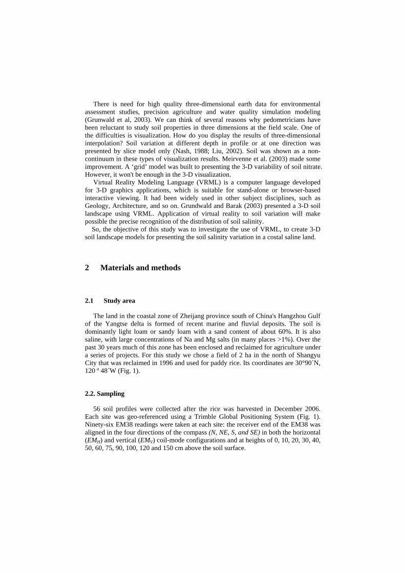
To show the x, y, and z dimension of VRML soil salinity models, we should build a 3-D coordinate system model. A polyhedron model was used to express the border of the study area, and the IndexedLineSet node was used to build the prototype. The coordinate was defined by the Coordinate node, and the values of the 3-D coordinate were set by the Field point. At last, for move, zoom in, zoom out, and rotate the prototype conveniently, a Transform group node was redefined. Part of the code as fellow: DEF box Transform {

translation 0 0 0

scale 1 1 1

rotation 0 0 1 1

children [

Shape {

appearance DEF box_app Appearance {

material Material {emissiveColor 1 1 1 } }

geometry IndexedLineSet {

coord Coordinate {

point [

224.25 578.50 -57.62,

406.84 578.50 -57.62,

406.84 750.25 -57.62,

……] }

coordIndex [

0, 1, -1,

2, 3, -1,

4, 5, -1,

……] }}]}

Fig. 3. Virtual environment of coordinate system

The virtual environment of the coordinate system was shown in Fig. 3. Since the VRML code is hierarchical, portable and modular, the model can be used in the fellow ECa visualization.

3.2. Visualization of ECa Profiles

The linear model inversed ECa at the depth of 5, 15, 25, 35, 45, 55, 67.5, 82.5, 95 and 110 cm is the datum resources of 3-D variation. The sphere prototype was

designed to express these 460 inversed sites. One site was defined by one Transform node. The Shape node was component by several fields, such as appearance Apperance, geometry, and Sphere_s. The ECa value was rendered by the color, and the diffuseColor field which decided by three values was used for the visualization of soil ECa models. In addition, the settled value of diffuseColor field is same as the legend value which versus the same ECa. Part of the code as fellow: DEF post_samples_Samples Transform {

translation -6.98522 -8.18395 25.6605

scale 0.0381559 0.0381560 0.0381559

rotation -0.98782 0.10516 0.11465 1.2187

children [

Transform {

translation 321 740.5 -2.5

children [

Shape {

appearance Appearance {

material Material {

ambientIntensity 0.301

diffuseColor 0 0.028 0.7

} }

geometry DEF _s Sphere {

radius 2

} } ] }

……}

Fig. 4. Visualization of ECa profiles

The ECa profiles were shown in Fig. 4. The disturibution of ECa can be seen more clearly in 3-D space. The higher ECa, the higher the salinity is. The deeper the depth is, the larger the soil average ECa is. The map of ECa displayed a spatial distribution with a high salinity level in the east corner and low salinity level in the west and northern corner of the field. Obviously, the salinity in the bottom of southeast is relative high in this study area.

3.3. Visualization of ECa 3-D variation

The plume model was adopted to express the 3-D ECa variation. The Indexedfaceset node was used to establish the surface of the plume. The same as the ECa profiles model, the ECa value was rendered by the color, and the diffuseColor field was used for the visualization of soil ECa models.

Fig. 5(a), (b), and (c) showed the volume of soil where the ECa was greater than 0 mSm-1, 170 mSm-1, and 300 mSm-1, respectively. The Anchor node acts as the trigger, helping us analyze the ECa change dynamically. For example, if we click the Fig. 5(a), the screen was cut from it to the Fig. 5(b). Part of the code as fellow: Anchor {

url "EC170.wrl" # EC170.wrl is the VRML

#program file name of Fig.5(b).

children [ …… #The program code of Figure

#5(a) should be include into ‘[]’

] }

(a) ECa>0 mSm-1

(b) ECa>170 mSm-1

(c) ECa>300 mSm-1

Fig. 5. Visualization of ECa variation

As expected, the prediction volume of soil shrinks as the specified ECa thresholds increased. This is a very important method which can be used to evaluate soil salinity in 3-D space. Obviously, the salinity in the bottom of southeast is relative high in this study area.

3.4. Communication on the WWW

The VRML programs made in this study were placed on a WWW server. The soil salinity model in this study can be opened and be accessed by anyone. Using WWW to transfer information to the public is considered as a very important and practical method, and the VRML soil landscape models are accessible via the WWW at http://agri.zju.edu.cn/vrml.html.

Fig. 6. Internet distribution interface of the ECa

4 Conclusions

In this study, it was summarized a procedure that from 3-D distributed sites to 3-D visualization salinity model.

The object-oriented 3-D graphics language VRML was used to create 3-D soil salinity models. The sphere and plume model was built for presenting the ECa sites and ECa variation, respectively. The VRML models presented a superior visualization of spatial distribution of ECa in 3-D space. It was shown that the field in the east corner and low salinity level in the west and northern corner of the field has a high salinity level. The salinity increased with the increase of the soil depth at the vertical direction.

VRML was so attractive for soil salinity modeling because: (1) it creates realistic 3-D virtual reality, (2) what is more important to us, the VRML models can be placed on the WWW. It is very convenient for the public to access the soil salinity information, and (3) soil salinity models have merit for soil information systems updating, helping for soil site-specific management.

We were able to create coherent 3-D ECa models using VRML. This study investigated relatively static ECa property; however, the potential to visualize 3-D transport processes within and on soils using animated VRML movie techniques is enormous.

5 Acknowledgements

The author acknowledges the funding of this work by the National Natural Science Foundation of China (No. 40871100, No. 40701007) and the National Science and Technology Support Program of China (No. 2006BAD10A09).

References

1. Ames, A. L., Nadeau, D.R., Moreland, J.L.: VRML 2.0 Sourcebook. John Wiley and Sons, Inc., New York (1997)

2. Carey, R., Bell, G.: The annotated VRML97 reference manual. Addison Wesley Longman, Inc., MA(1997)

3. Liu, W. C., Jang, C. S., Chen, S. C.: Three-dimensional spatial variability of hydraulic conductivity in the Choushui River alluvial fan, Taiwan, Environ. Geol. 43, 48--56 (2002)

4. Amezketa E.: An Integrated Methodology for Assessing Soil Salinization, a Pre-condition for Land Desertification, J. Arid Environ. 67, 594--606(2006)

5. Li, H. Y., Shi, Z., Tang, H. L.: Research on three-dimension spatial variability of soil electrical conductivity of coastal saline land using 3D ordinary kriging method, Acta Pedologica Sinica, 47, 359--363(2010)

6. Li, H. Y., Shi, Z., Cheng, J. L.: Inversion of Soil Conductivity Profiles Based On EM38 Apparent Electrical Conductivity, Scientia Agric. Sinica, 41, 95--302(2008)

7. Lemay, L., Couch, J., Murdock, K.: 3D graphics and VRML 2. Sams.net Publ., Indianapolis, IN(1999)

8. Oliver M. A., Webster, R.: The Elucidation of Soil Pattern in the Wyre Forest of the West Midlands, England. II. Spatial Distribution, Eur. J. Soil Sci., 38, 293--307(2006)

9. Nash, M. H. , Daugherty, L. A., Wierenga, P. J.: Horizontal and vertical kriging of soil properties along a transect in southern New Mexico, SSSAJ, 52, 1086--1090(1988)

10. Meirvenne, M. V., Maes, K., Hofman, G.: Three-dimensional Variability of Soil Nitrate-nitrogen In an Agricultural Field, Biol. Fertil. Soils, 37, 147--153(2003)

11. Grunwald, S., Barak, P.: 3D geographic reconstruction and visualization techniques applied to land resource management, Transactions in GIS. 7(2), 231—241(2003)

12. Yu, T. H., Shi, C. X., Wu, Y. W.: Observation on Salt Spots in Coastal Land and Study on Tolerance of Barley and Cotton to Salt, J. Zhejiang Agri. Univ. 22, 201--204 (1996)