This work is licensed under a Creative Commons...
202
This work is licensed under a Creative Commons Attribution-NonCommercial-ShareAlike License . Your use of this material constitutes acceptance of that license and the conditions of use of materials on this site. Copyright 2006, The Johns Hopkins University and John McGready. All rights reserved. Use of these materials permitted only in accordance with license rights granted. Materials provided “AS IS”; no representations or warranties provided. User assumes all responsibility for use, and all liability related thereto, and must independently review all materials for accuracy and efficacy. May contain materials owned by others. User is responsible for obtaining permissions for use from third parties as needed.
Transcript of This work is licensed under a Creative Commons...
This work is licensed under a Creative Commons Attribution-NonCommercial-ShareAlike License. Your use of this material constitutes acceptance of that license and the conditions of use of materials on this site.
Copyright 2006, The Johns Hopkins University and John McGready. All rights reserved. Use of these materials permitted only in accordance with license rights granted. Materials provided “AS IS”; no representations or warranties provided. User assumes all responsibility for use, and all liability related thereto, and must independently review all materials for accuracy and efficacy. May contain materials owned by others. User is responsible for obtaining permissions for use from third parties as needed.
Comparing Proportions Between Two Independent Populations
John McGreadyJohns Hopkins University
Lecture Topics
CI’s for difference in proportions between two independent populationsLarge sample methods for comparing proportions between two populations– Normal method– Chi-squared testFisher’s exact testRelative risk
3
Section A
The Two Sample Z-Test for Comparing Proportions Between
Two Independent Populations
Comparing Two Proportions
We will motivate by using data from the Pediatric AIDS Clinical Trial Group (ACTG) Protocol 076 Study Group1
1 Conner, E., et al. Reduction of Maternal-Infant Transmission of Human Immunodeficiency Virus Type 1 with Zidovudine Treatment, New England Journal of Medicine 331: 18 Continued 5
Comparing Two Proportions
Study Design– “We conducted a randomized, double-
blinded, placebo-controlled trial of the efficacy and safety of zidovudine (AZT) in reducing the risk of maternal-infant HIV transmission”
– 363 HIV infected pregnant women were randomized to AZT or placebo
Continued 6
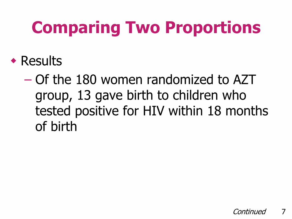
Comparing Two Proportions
Results– Of the 180 women randomized to AZT
group, 13 gave birth to children who tested positive for HIV within 18 months of birth
Continued 7
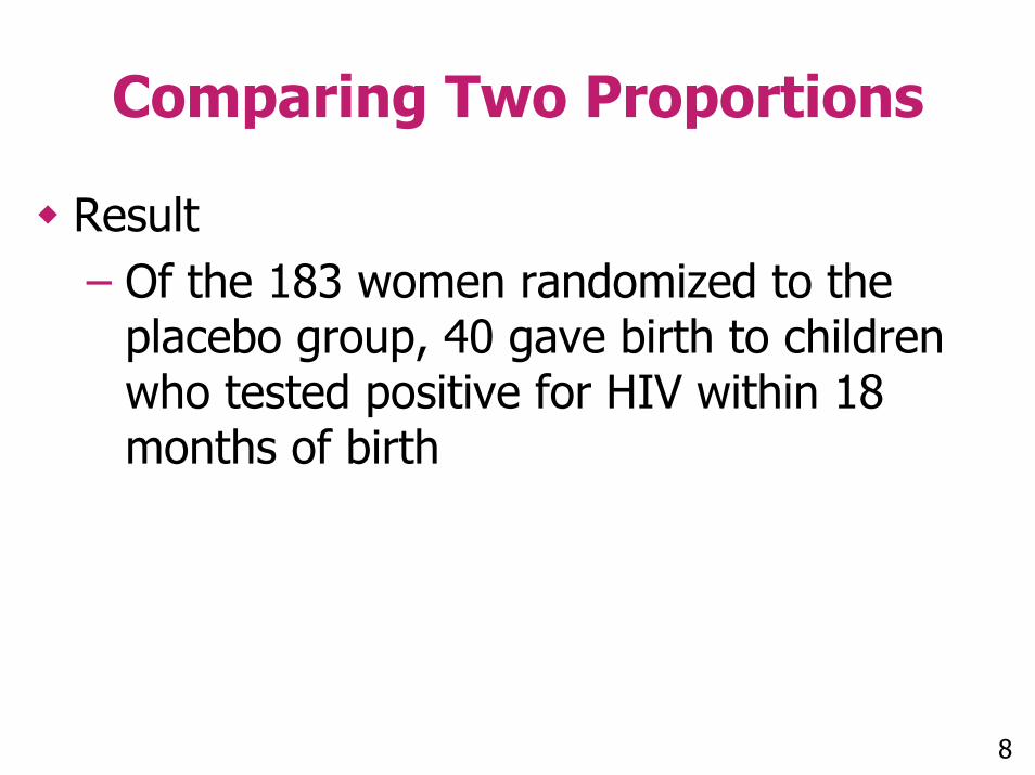
Comparing Two Proportions
Result– Of the 183 women randomized to the
placebo group, 40 gave birth to children who tested positive for HIV within 18 months of birth
8
Notes on Design
Random assignment of Tx– Helps insure two groups are comparable– Patient and physician could not request
particular Tx
Continued 9
Notes on Design
Double blind– Patient and physician did not know Tx
assignment
10

HIV Transmission Rates
AZT
Placebo
072.018013ˆ ==AZTp
219.018340ˆ ==PLACp
Continued 11
HIV Transmission Rates
Note—these are NOT the true population parameters for the transmission rates, they are estimates based on our two samples
Continued 12
HIV Transmission Rates
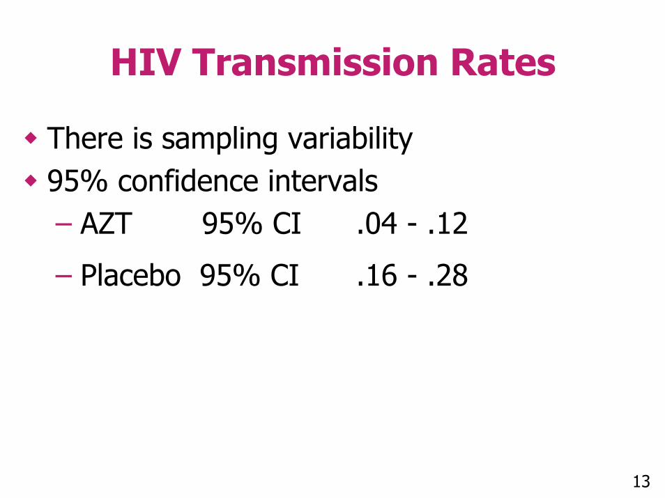
There is sampling variability95% confidence intervals– AZT 95% CI .04 - .12
– Placebo 95% CI .16 - .28
13
95% CIs for HIV Transmission Rates
AZT
Placebo
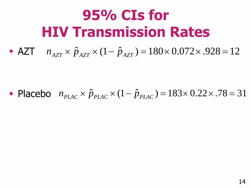
12928.072.0180)ˆ1(ˆ =××=−×× AZTAZTAZT ppn
3178.22.0183)ˆ1(ˆ =××=−×× PLACPLACPLAC ppn
14
HIV Transmission Rates
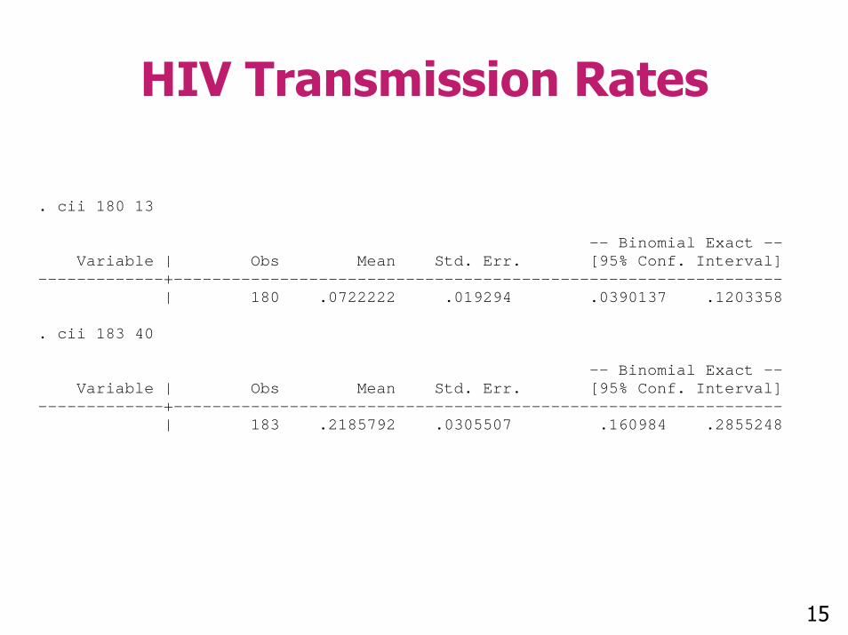
. cii 180 13 -- Binomial Exact -- Variable | Obs Mean Std. Err. [95% Conf. Interval] -------------+--------------------------------------------------------------- | 180 .0722222 .019294 .0390137 .1203358 . cii 183 40 -- Binomial Exact -- Variable | Obs Mean Std. Err. [95% Conf. Interval] -------------+--------------------------------------------------------------- | 183 .2185792 .0305507 .160984 .2855248
15
Notes on HIV Transmission Rates
Is the difference significant, or can it be explained by chance?Since CI’s do not overlap suggests significant difference– Can we compute a confidence interval on
the difference in proportions?– Can we compute a p-value?
16
Sampling Distribution of the Difference in Sample Means
Since we have large samples we know the sampling distributions of the sample proportions in both groups are approximately normalIt turns out the difference of quantities, which are (approximately) normally distributed, are also normally distributed
Continued 17
Sampling Distribution of the Difference in Sample Means
So, the big news is . . .– The sampling distribution of the difference
of two sample proportions, each based on large samples, approximates a normal distribution
– This sampling distribution is centered at the true (population) difference, P1 - P2
18

Simulated Sampling Distribution of Sample Proportion
19
05
1015
Per
cent
age
of S
ampl
es
0 . 05 .1 .15 .2 .25 .3 .35S am ple P roportion HIV In fec ted C h ild ren
A ZT Group, n = 180S imula te d S a mpling D is tr ibutio n, P ro po rtio n HIV Infe c te d C hildre n
Continued
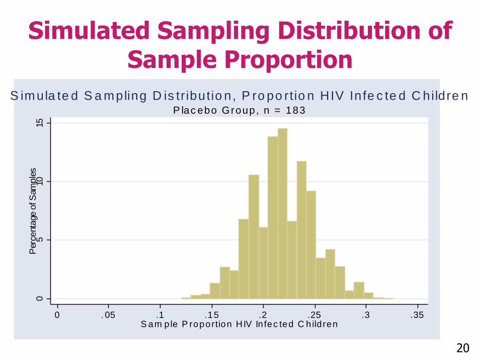
Simulated Sampling Distribution of Sample Proportion
20
05
1015
Per
cent
age
of S
ampl
es
0 . 05 .1 .15 .2 .25 .3 .35S am ple P roportion HIV In fec ted C h ild ren
P lac ebo Group, n = 183S imula te d S a mpling D is tr ibutio n, P ro po rtio n HIV Infe c te d C hildre n

Simulated Sampling Distribution Difference in Sample Proportions
05
1015
20Pe
rcen
tage
of S
ampl
es
0 .0 5 . 1 .1 5 .2 .2 5 .3 .3 5D if fe r e n c e in S a m p le P r o p o r t io n s H IV In fe c te d C h ild r e n
( P la c e b o - A Z T )S im u la t e d S a m p lin g D is t r i b u t io n , D i f f e r e n c e in P r o p o r t i o n s
21
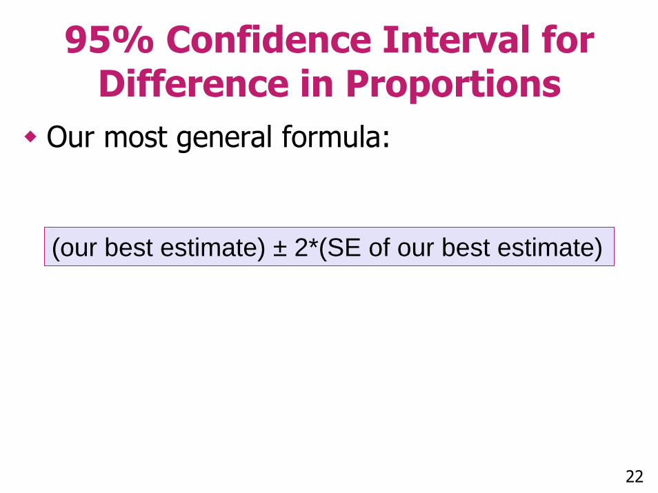
95% Confidence Interval for Difference in Proportions
Our most general formula:
(our best estimate) ± 2*(SE of our best estimate)
22

95% Confidence Interval for Difference in Means
Well, our best estimate for the mean difference would be :
Where . . .– = proportion HIV infected children in
AZT group– = proportion HIV infected children in
placebo group
1p̂
2p̂
21 ˆˆ pp −
Continued 23
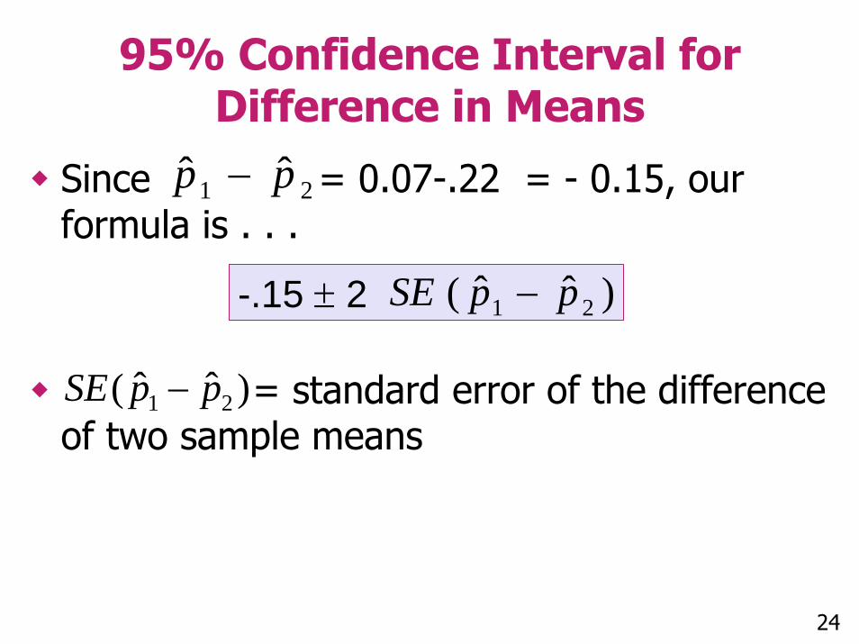
95% Confidence Interval for Difference in Means
Since = 0.07-.22 = - 0.15, our formula is . . .
= standard error of the difference of two sample means
21 ˆˆ pp −
-.15 ± 2 )ˆˆ( 21 ppSE −
)ˆˆ( 21 ppSE −
24
Two Independent Groups
Statisticians have developed formulas for the standard error of the difference– These formulas depend on sample sizes in
both groups and sample proportion in both groups
Continued 25
Two Independent Groups
The is greater than eitherthe or Why do you think this is?
)ˆˆ( 21 ppSE −)ˆ( 1pSE )ˆ( 2pSE
Continued 26

Two Independent Groups
In the example . . .
031.)ˆ(019.)ˆ(
036.)ˆˆ(
2
1
21
==
=−
pSEpSE
ppSE
27
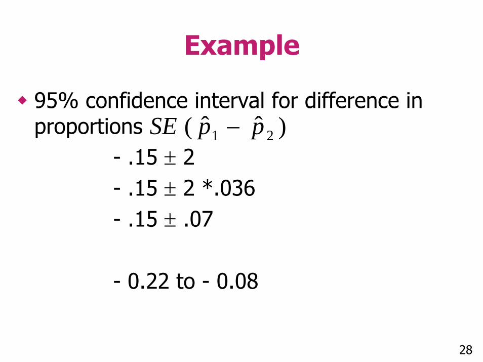
Example
95% confidence interval for difference in proportions
- .15 ± 2- .15 ± 2 *.036- .15 ± .07
- 0.22 to - 0.08
)ˆˆ( 21 ppSE −
28

Note
The confidence interval does not include 0
29
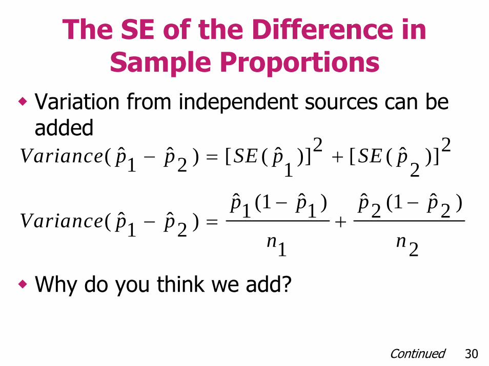
The SE of the Difference in Sample Proportions
Variation from independent sources can be added
Why do you think we add?
2
)2ˆ1(2ˆ
1
)1ˆ1(1ˆ)2ˆ1ˆ(
2)]2
ˆ([2)]1
ˆ([)2ˆ1ˆ(
n
pp
n
ppppVariance
pSEpSEppVariance
−+
−=−
+=−
Continued 30
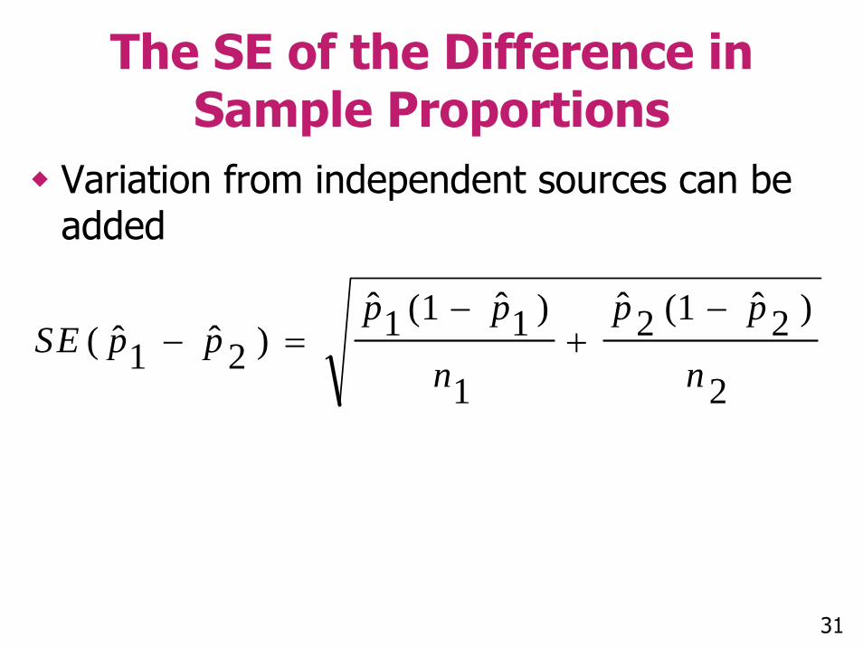
The SE of the Difference in Sample Proportions
Variation from independent sources can be added
2
)2ˆ1(2ˆ
1
)1ˆ1(1ˆ)2ˆ1ˆ(
n
pp
n
ppppSE
−+
−=−
31
Principle
Formula depends on n1, n2, There are other slightly different equations for (e.g. Altman, p.234)But they all give similar answers
)ˆˆ( 21 ppSE −
21 ˆ,ˆ pp
32

Simple Approximation Method to Compare Proportions
Hypotheses
H0: P1 = P2
Ha: P1 ≠ P2
Continued 33

Simple Approximation Method to Compare Proportions
Hypotheses
H0: P1 - P2 = 0
Ha: P1 - P2 ≠ 0
Continued 34

Simple Approximation Method to Compare Proportions
Recall the general “recipe” for hypothesis testing:
1. State null and alternative hypotheses2. Calculate test statistic based on sample3. Compare test statistic to appropriate
distribution to get p-value
Continued 35
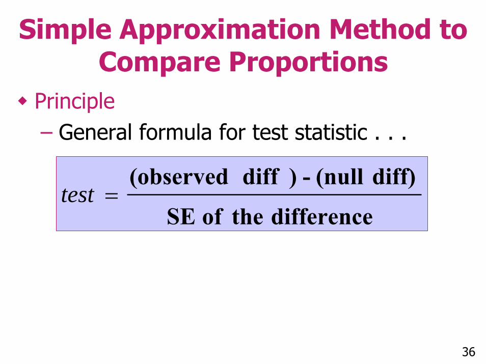
Simple Approximation Method to Compare Proportions
Principle– General formula for test statistic . . .
difference the of SE
diff) (null - ) diff (observed=test
36

Comparing Proportions
But since null difference is zero, this reduces to . . .
difference the of SE
) diff (observed=test
Continued 37
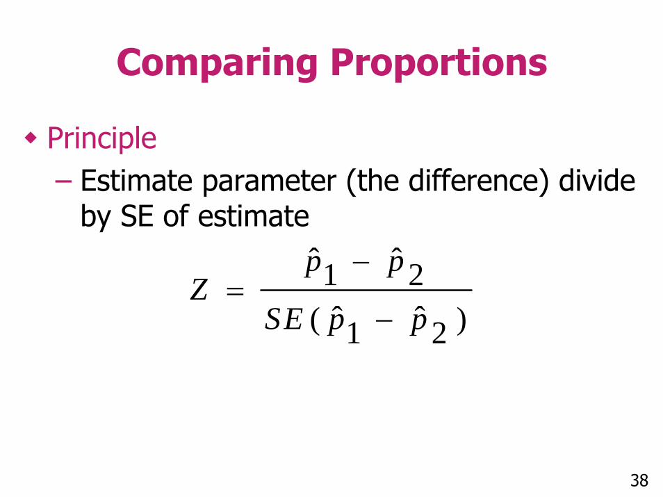
Comparing Proportions
Principle– Estimate parameter (the difference) divide
by SE of estimate
)2ˆ1ˆ(2ˆ1ˆ
ppSE
ppZ
−
−=
38
Two-Sample z-test for Comparing Proportions
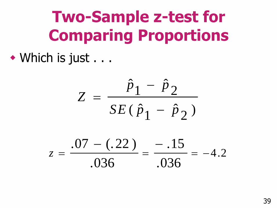
Which is just . . .
)2ˆ1ˆ(
2ˆ1ˆ
ppSE
ppZ
−
−=
2.4036.
15.036.
)22(.07.−===
−−z
39

Note
This is a two sample z-test for comparing two proportions– The value z = - 4.2 is the test statisticWe calculate a p-value which is the probability of obtaining a test statistic as extreme as we did if H0 was true
40
How Are p-values Calculated?
Is a result 4.2 standard errors below 0 unusual?– It depends on what kind of distribution we
are dealing with
Continued 41
How Are p-values Calculated?
The p-value is the probability of getting a test statistic as or more extreme than what you observed (- 4.2) by chance if H0 was trueThe p-value comes from the sampling distribution of the difference in two sample proportions
42
Sampling Distribution
What is sampling distribution of the difference in sample proportions? – If both groups are large then this
distribution is approximately normal
43
AZT Study
So, since both our samples are large our sampling distribution will be approximately normal– This sampling distribution will be centered
at true difference, P1 - P2
– Under null hypothesis, this true difference is 0
Continued 44
AZT Study
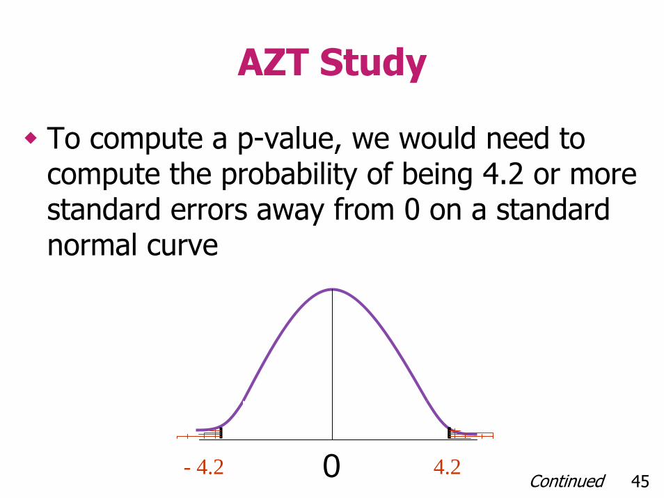
To compute a p-value, we would need to compute the probability of being 4.2 or more standard errors away from 0 on a standard normal curve
0- 4.2 4.2Continued 45
AZT Study
If we were to look this up on a normal table, we would find a very low p-value (p < .001)
46
Notes
This method is also essentially equivalent to the chi-square (χ2) method– Gives about the same answer – (p-value) – We will discuss chi-square method next
47
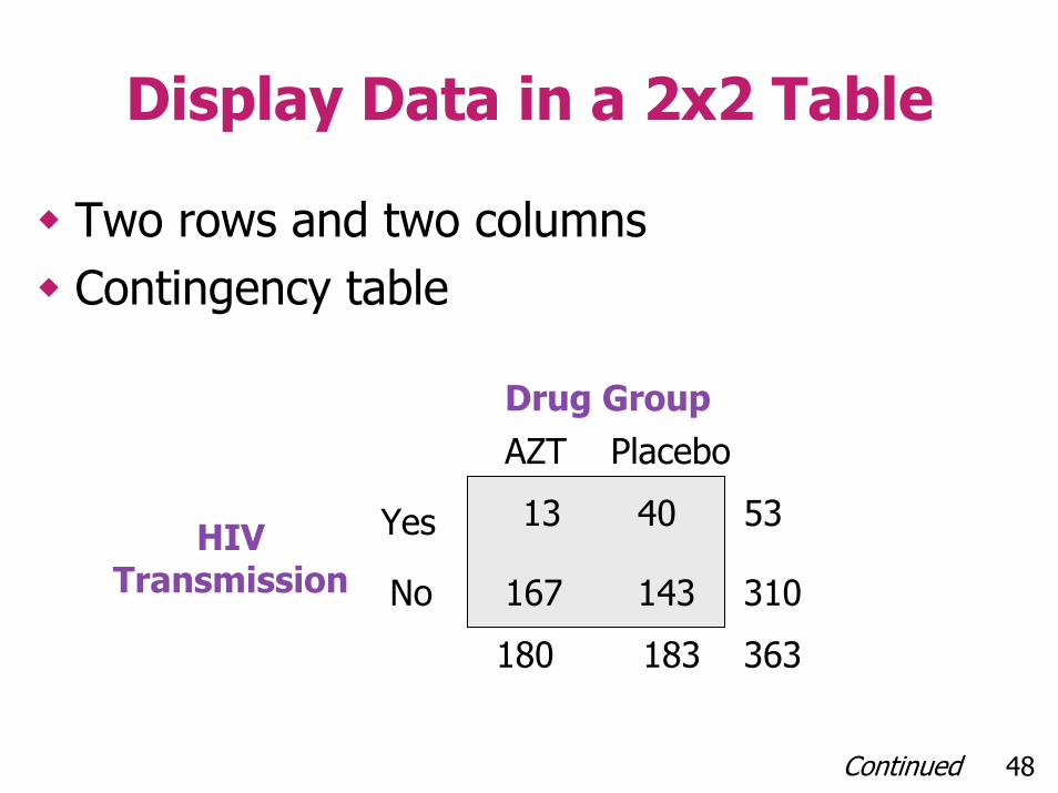
Display Data in a 2x2 Table
Two rows and two columnsContingency table
AZT Placebo
Yes
No
Drug Group
HIVTransmission
13 40
167 143
180 183
53
310
363
Continued 48
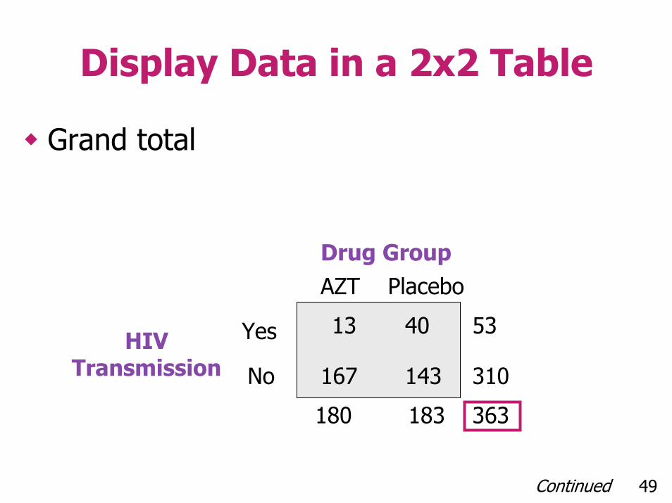
Display Data in a 2x2 Table
Grand total
AZT Placebo
Yes
No
Drug Group
HIVTransmission
13 40
167 143
180 183
53
310
363
Continued 49

Display Data in a 2x2 Table
Column totals
AZT Placebo
Yes
No
Drug Group
HIVTransmission
13 40
167 143
180 183
53
310
363
Continued 50
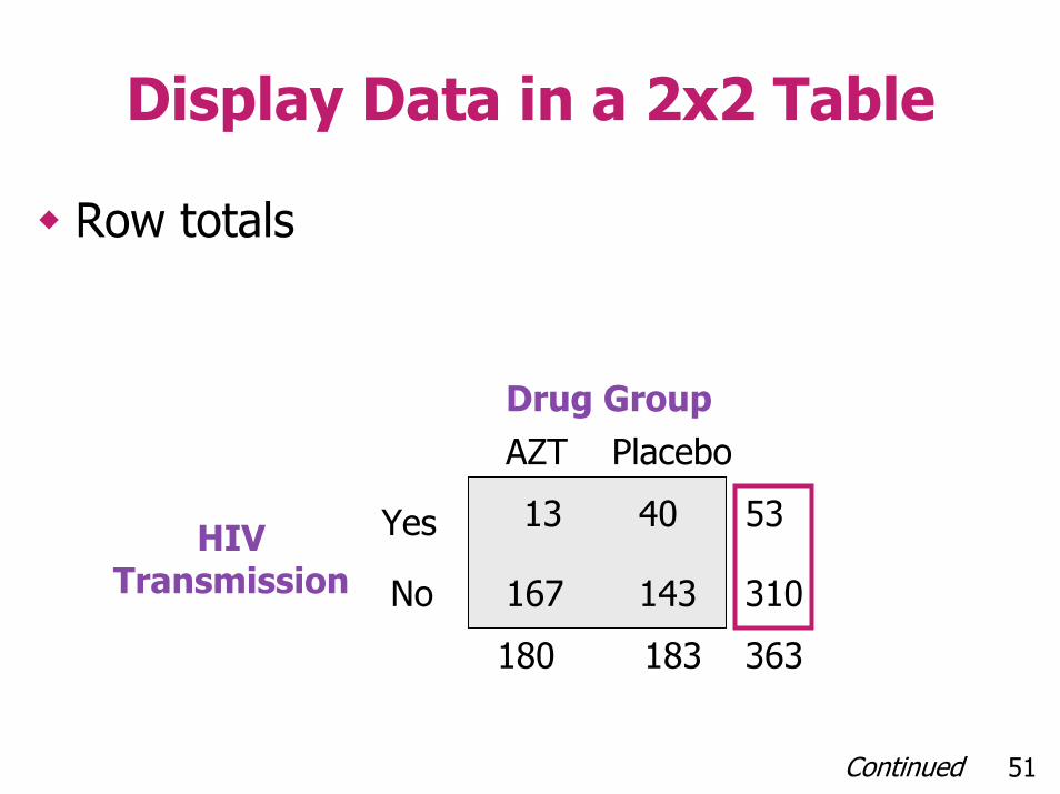
Display Data in a 2x2 Table
Row totals
AZT Placebo
Yes
No
Drug Group
HIVTransmission
13 40
167 143
180 183
53
310
363
Continued 51
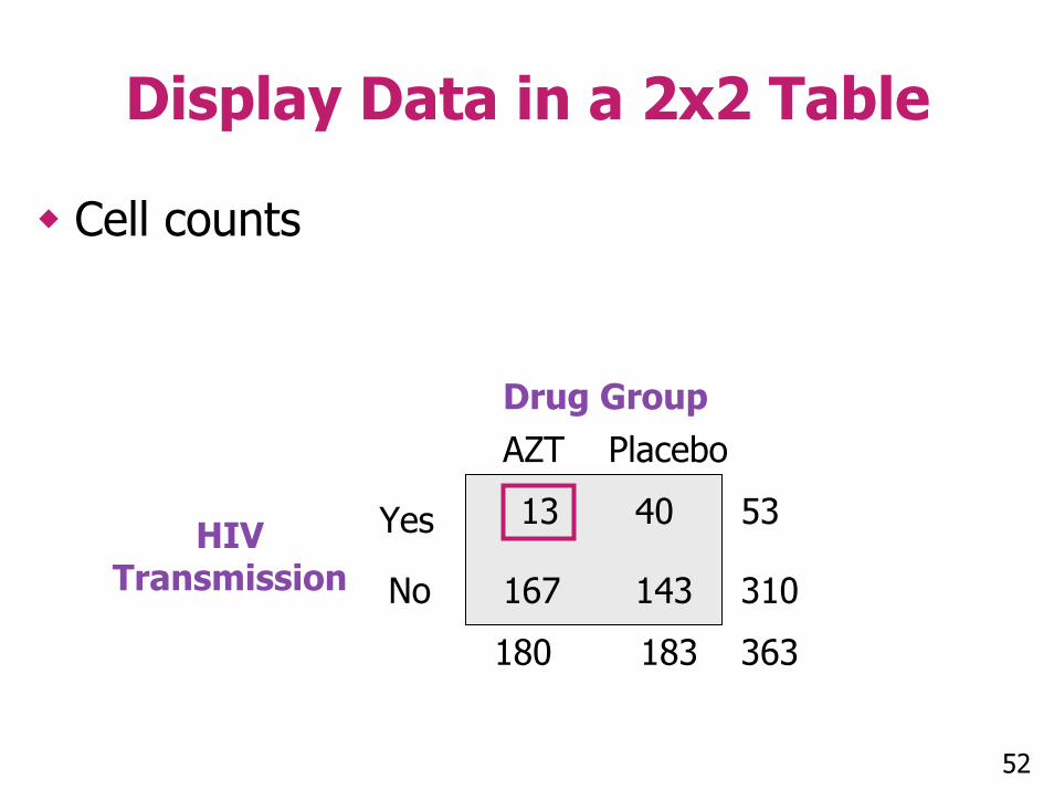
Display Data in a 2x2 Table
Cell counts
AZT Placebo
Yes
No
Drug Group
HIVTransmission
13 40
167 143
180 183
53
310
363
52
Using Stata
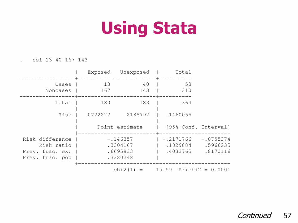
We can get Stata to give us a 95% CI for the difference in proportions, and a p-value by using the csi command
Continued 53
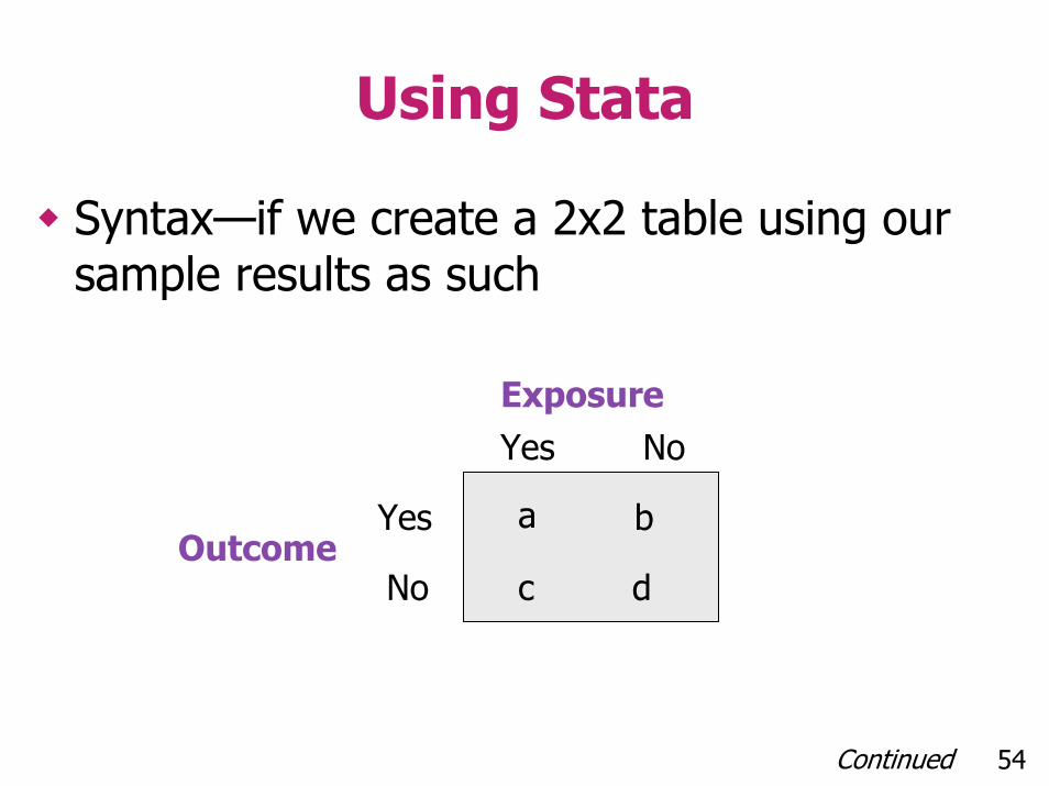
Using Stata
Syntax—if we create a 2x2 table using our sample results as such
ExposureYes No
Yes a b
c dOutcome
No
Continued 54

Using Stata
Syntax:– csi a b c d
Continued 55

Using Stata
2x2 table formed using results from a Maternal-Infant Transmission Study
Drug GroupAZT Placebo
5313 40
167 143
YesHIVTransmission No 210
180 183 263
Continued 56
Using Stata
. csi 13 40 167 143 | Exposed Unexposed | Total -----------------+------------------------+---------- Cases | 13 40 | 53 Noncases | 167 143 | 310 -----------------+------------------------+---------- Total | 180 183 | 363 | | Risk | .0722222 .2185792 | .1460055 | | | Point estimate | [95% Conf. Interval] |------------------------+---------------------- Risk difference | -.146357 | -.2171766 -.0755374 Risk ratio | .3304167 | .1829884 .5966235 Prev. frac. ex. | .6695833 | .4033765 .8170116 Prev. frac. pop | .3320248 | +----------------------------------------------- chi2(1) = 15.59 Pr>chi2 = 0.0001
Continued 57
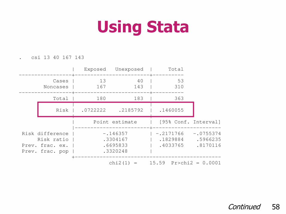
Using Stata
. csi 13 40 167 143 | Exposed Unexposed | Total -----------------+------------------------+---------- Cases | 13 40 | 53 Noncases | 167 143 | 310 -----------------+------------------------+---------- Total | 180 183 | 363 | | Risk | .0722222 .2185792 | .1460055 | | | Point estimate | [95% Conf. Interval] |------------------------+---------------------- Risk difference | -.146357 | -.2171766 -.0755374 Risk ratio | .3304167 | .1829884 .5966235 Prev. frac. ex. | .6695833 | .4033765 .8170116 Prev. frac. pop | .3320248 | +----------------------------------------------- chi2(1) = 15.59 Pr>chi2 = 0.0001
Continued 58

Using Stata
. csi 13 40 167 143 | Exposed Unexposed | Total -----------------+------------------------+---------- Cases | 13 40 | 53 Noncases | 167 143 | 310 -----------------+------------------------+---------- Total | 180 183 | 363 | | Risk | .0722222 .2185792 | .1460055 | | | Point estimate | [95% Conf. Interval] |------------------------+---------------------- Risk difference | -.146357 | -.2171766 -.0755374 Risk ratio | .3304167 | .1829884 .5966235 Prev. frac. ex. | .6695833 | .4033765 .8170116 Prev. frac. pop | .3320248 | +----------------------------------------------- chi2(1) = 15.59 Pr>chi2 = 0.0001
Continued 59
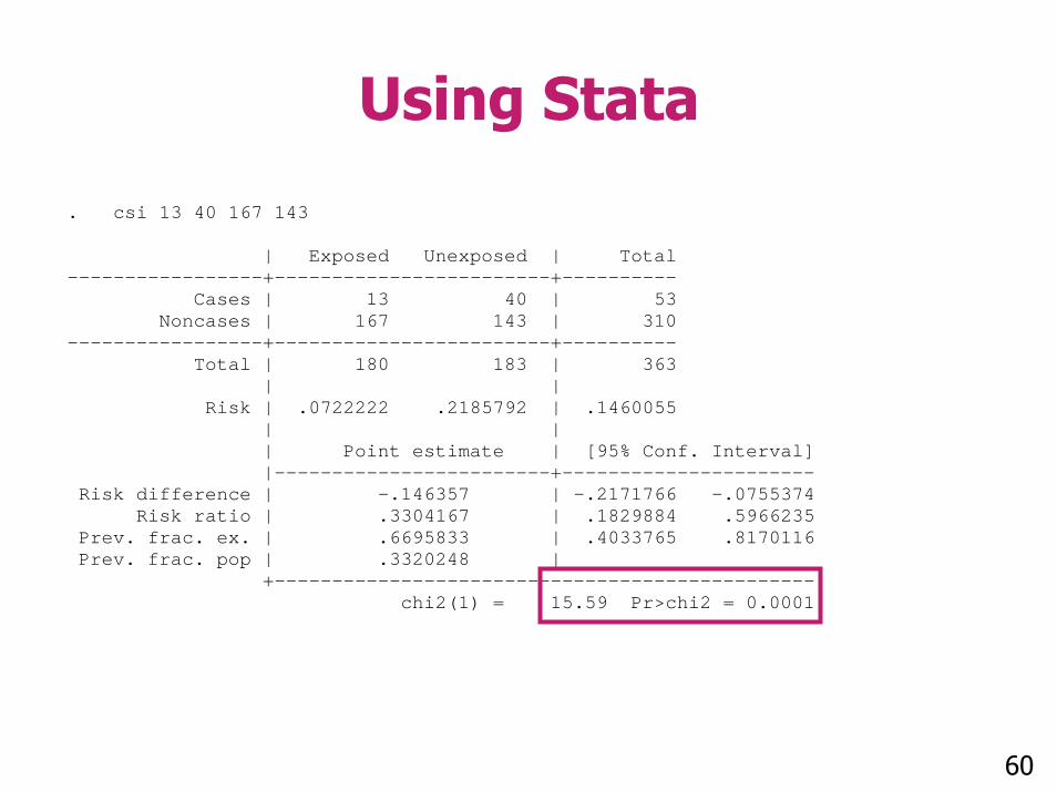
Using Stata
. csi 13 40 167 143 | Exposed Unexposed | Total -----------------+------------------------+---------- Cases | 13 40 | 53 Noncases | 167 143 | 310 -----------------+------------------------+---------- Total | 180 183 | 363 | | Risk | .0722222 .2185792 | .1460055 | | | Point estimate | [95% Conf. Interval] |------------------------+---------------------- Risk difference | -.146357 | -.2171766 -.0755374 Risk ratio | .3304167 | .1829884 .5966235 Prev. frac. ex. | .6695833 | .4033765 .8170116 Prev. frac. pop | .3320248 | +----------------------------------------------- chi2(1) = 15.59 Pr>chi2 = 0.0001
60
Summary: AZT Study
Statistical Method– “We conducted a randomized, double-
blind, placebo-controlled trial of the efficacy and safety of zidovudine (AZT) in reducing the risk of maternal-infant HIV transmission”
Continued 61
Summary: AZT Study
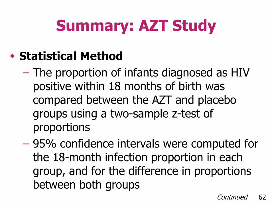
Statistical Method– The proportion of infants diagnosed as HIV
positive within 18 months of birth was compared between the AZT and placebo groups using a two-sample z-test of proportions
– 95% confidence intervals were computed for the 18-month infection proportion in each group, and for the difference in proportions between both groups
Continued 62
Summary: AZT Study
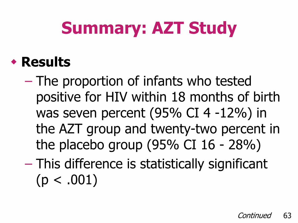
Results– The proportion of infants who tested
positive for HIV within 18 months of birth was seven percent (95% CI 4 -12%) in the AZT group and twenty-two percent in the placebo group (95% CI 16 - 28%)
– This difference is statistically significant (p < .001)
Continued 63

Summary: AZT Study
Results– The study results estimate the decrease in
the proportion of HIV positive infants born to HIV positive mothers attributable to AZT to possibly be as low as 8% and as high as 22%
64
Section A
Practice Problems

Practice Problems
A study was performed on a representative sample of 258 intravenous drug users (IVDUs)Of particular interest to the researchers were factors which may influence the risk of contracting tuberculosis amongst IVDUs1
Source: 1 Based on data reported in: Graham, N., et al. Prevalence of Tuberculin Positivity and Skin Test Anergy in HIV-1-Seropisitive and Seronegative Intravenous Drug Users, Journal of the American Medical Association 267: 3. Continued 66
Practice Problems
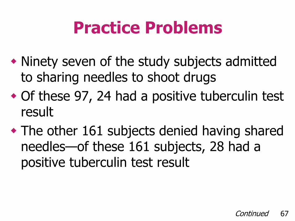
Ninety seven of the study subjects admitted to sharing needles to shoot drugsOf these 97, 24 had a positive tuberculin test resultThe other 161 subjects denied having shared needles—of these 161 subjects, 28 had a positive tuberculin test result
Continued 67
Practice Problems
a) Using the study results, construct a 95% confidence interval for the difference in the proportion of tuberculosis infected IVDUS who shared needles as compared to IVDUS who did not share needles
Continued 68
Practice Problems
b) What is the p-value for testing the null hypothesis that the proportions of individuals testing positive for tuberculosis are the same between the two groups of IVDUs?
Continued 69
Practice Problems
c) Does this study suggest a relationship between tuberculosis infection and needle sharing in IVDUs?
70
Section A
Practice Problems Solutions
Practice Problems
A study was performed on a representative sample of 258 intravenous drug users (IVDUs)Of particular interest to the researchers were factors which may influence the risk of contracting tuberculosis amongst IVDUs1
Source: 1 Based on data reported in: Graham, N., et al. Prevalence of Tuberculin Positivity and Skin Test Anergy in HIV-1-Seropisitive and Seronegative Intravenous Drug Users, Journal of the American Medical Association 267: 3. Continued 72

Practice Problems
Ninety seven of the study subjects admitted to sharing needles to shoot drugsOf these 97, 24 had a positive tuberculin test resultThe other 161 subjects denied having shared needles—of these 161 subjects, 28 had a positive tuberculin test result
Continued 73

Practice Problems
a) Using the study results, construct a 95% confidence interval for the difference in the proportion of tuberculosis infected IVDUS who shared needles as compared to IVDUS who did not share needles
Continued 74

Practice Problems
First, it may prove helpful to arrange the study results in a 2x2 contingency table
Yes No
Yes
No
Share Needles?
TB
Positive?
24 28
73 133
97 161
52
206
258
Continued 75
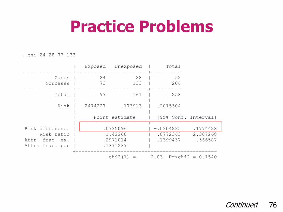
Practice Problems. csi 24 28 73 133 | Exposed Unexposed | Total -----------------+------------------------+---------- Cases | 24 28 | 52 Noncases | 73 133 | 206 -----------------+------------------------+---------- Total | 97 161 | 258 | | Risk | .2474227 .173913 | .2015504 | | | Point estimate | [95% Conf. Interval] |------------------------+---------------------- Risk difference | .0735096 | -.0304235 .1774428 Risk ratio | 1.42268 | .8772363 2.307268 Attr. frac. ex. | .2971014 | -.1399437 .566587 Attr. frac. pop | .1371237 | +----------------------------------------------- chi2(1) = 2.03 Pr>chi2 = 0.1540
Continued 76

Practice Problems
b) What is the p-value for testing the null hypothesis that the proportions of individuals testing positive for tuberculosis are the same between the two groups of IVDUs?
Continued 77
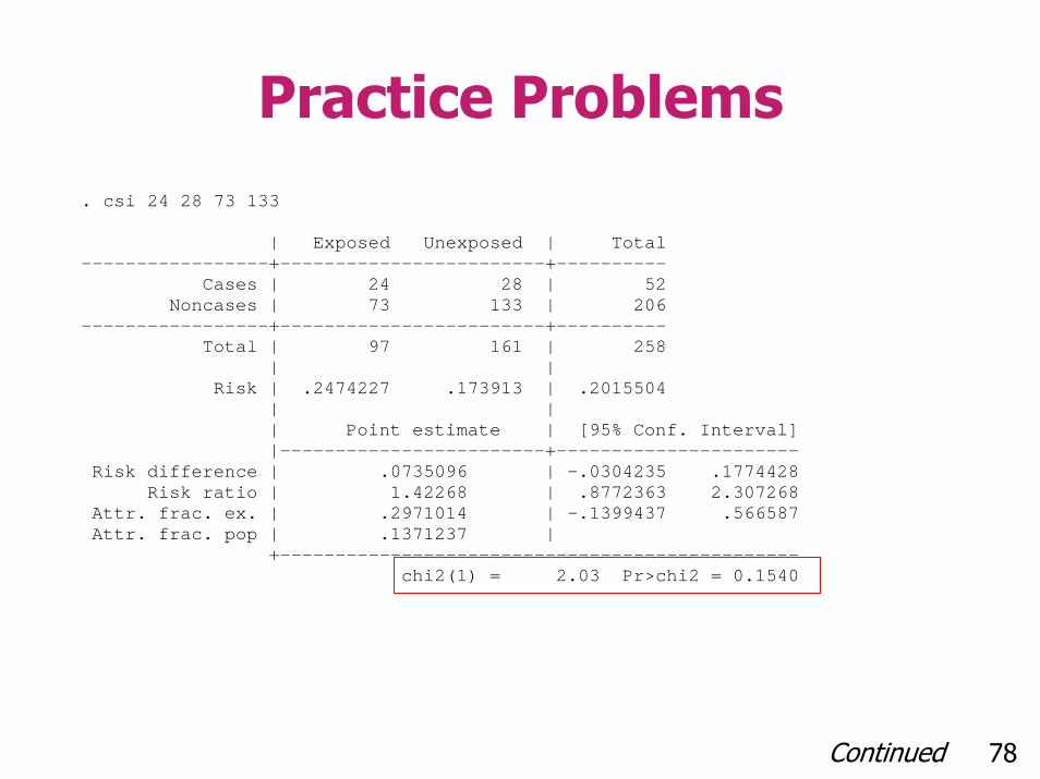
Practice Problems. csi 24 28 73 133 | Exposed Unexposed | Total -----------------+------------------------+---------- Cases | 24 28 | 52 Noncases | 73 133 | 206 -----------------+------------------------+---------- Total | 97 161 | 258 | | Risk | .2474227 .173913 | .2015504 | | | Point estimate | [95% Conf. Interval] |------------------------+---------------------- Risk difference | .0735096 | -.0304235 .1774428 Risk ratio | 1.42268 | .8772363 2.307268 Attr. frac. ex. | .2971014 | -.1399437 .566587 Attr. frac. pop | .1371237 | +----------------------------------------------- chi2(1) = 2.03 Pr>chi2 = 0.1540
Continued 78

Practice Problems
c) Does this study suggest a relationship between tuberculosis infection and needle sharing in IVDUs?
79
Section B
The Chi-Squared Test
Hypothesis Testing Problem
H0: P1 = P2 (P1 - P2 = 0)Ha: P1 ≠ P2 (P1 - P2 ≠ 0)– In the context of the 2x2 table, this is
testing whether there is a relationship between the rows (HIV status) and columns (treatment type)
81
Statistical Test Procedures
(Pearson’s) Chi-Square Test (χ2)– Calculation is easy (can be done by hand)Works well for big sample sizes
82
The Chi-Square Approximate Method
Gives (essentially) same p-value as z-test for comparing two proportionsCan be extended to compare proportions between more than two independent groups in one test
83Continued
The Chi-Square Approximate Method
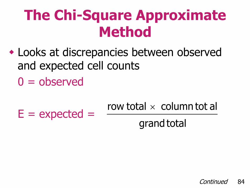
Looks at discrepancies between observed and expected cell counts0 = observed
E = expected =total grand
altot column total row ×
84Continued
The Chi-Square Approximate Method
Expected refers to the values for the cell counts that would be expected if the null hypothesis is true– The expected values if the proportions are
equal
85Continued
The Chi-Square Approximate Method
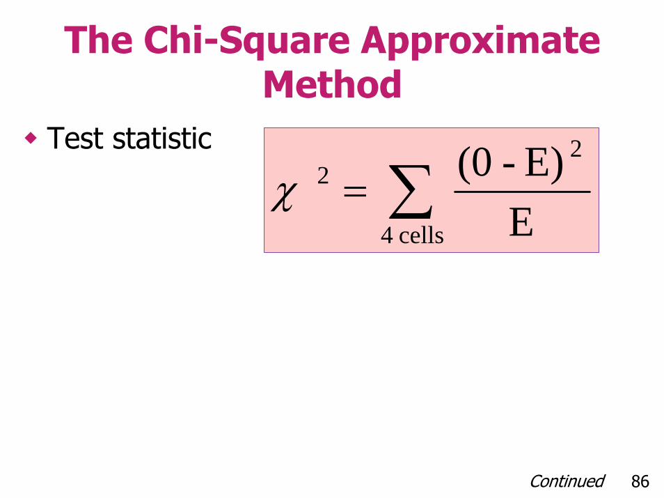
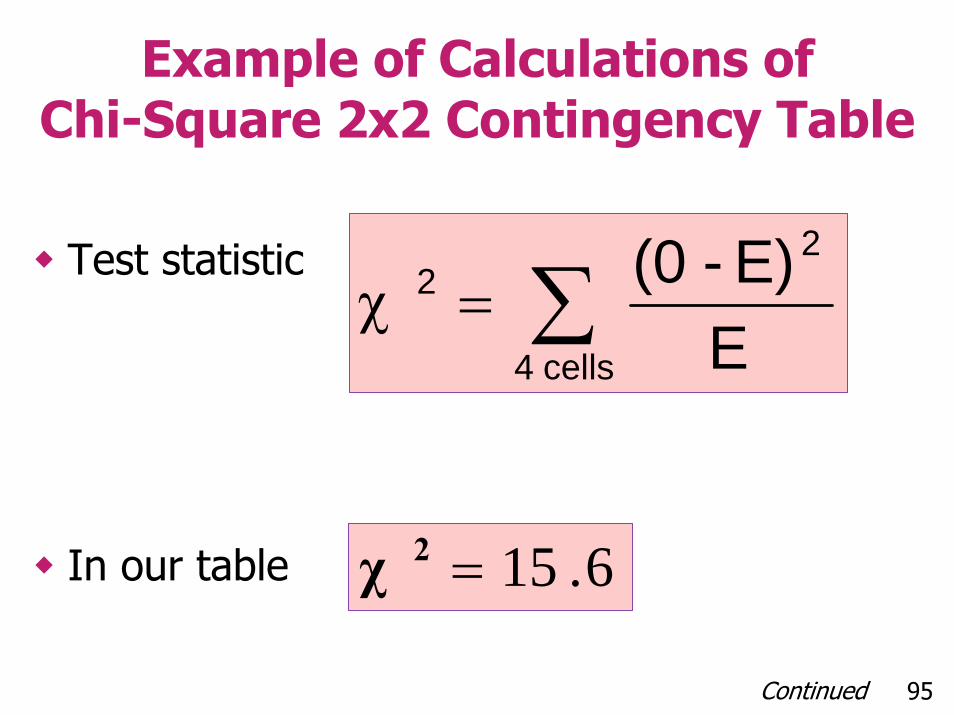
Test statistic
∑=cells 4
22
EE)-(0 χ
86Continued
The Chi-Square Approximate Method
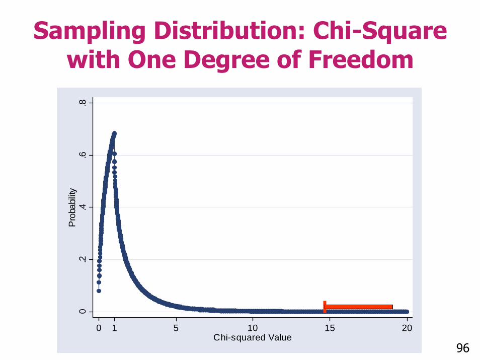
The sampling distribution of this statistic when the null is a chi-square distribution with one degree of freedom We can use this to determine how likely it was to get such a big discrepancy between the observed and expected by chance alone
87

Sampling Distribution: Chi-Square with One Degree of Freedom
0.2
.4.6
.8P
roba
bility
0 1 5 10 15 20Chi-squared Value 88
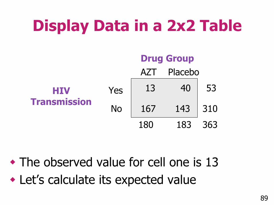
Display Data in a 2x2 Table
AZT Placebo
Yes
No
Drug Group
HIVTransmission
13 40
167 143
180 183
53
310
363
The observed value for cell one is 13Let’s calculate its expected value
89
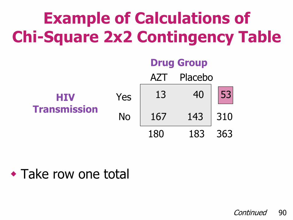
Example of Calculations of Chi-Square 2x2 Contingency Table
AZT Placebo
Yes
No
Drug Group
HIVTransmission
13 40
167 143
180 183
53
310
363
Take row one total
90Continued
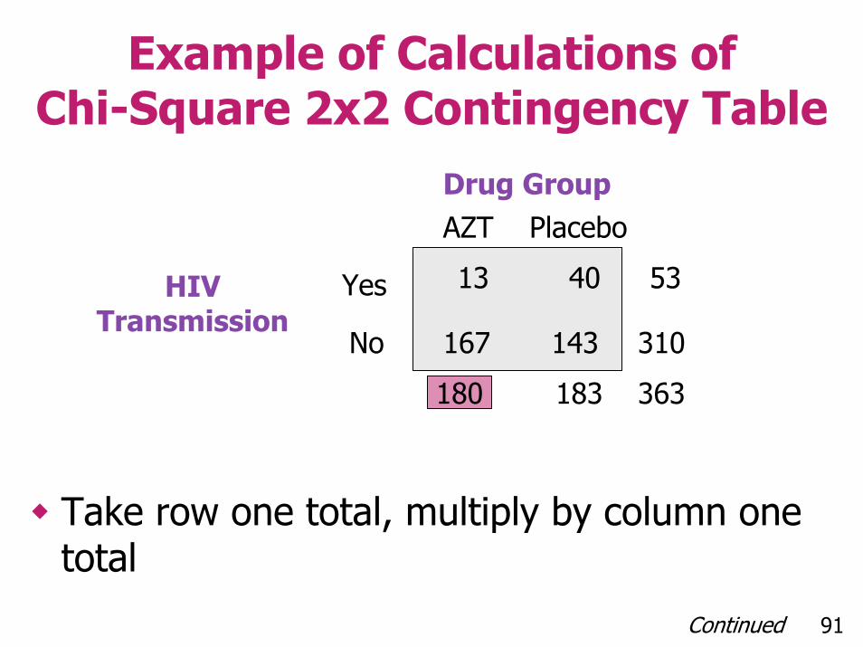
Example of Calculations of Chi-Square 2x2 Contingency Table
Take row one total, multiply by column one total
AZT Placebo
Yes
No
Drug Group
HIVTransmission
13 40
167 143
180 183
53
310
363
91Continued
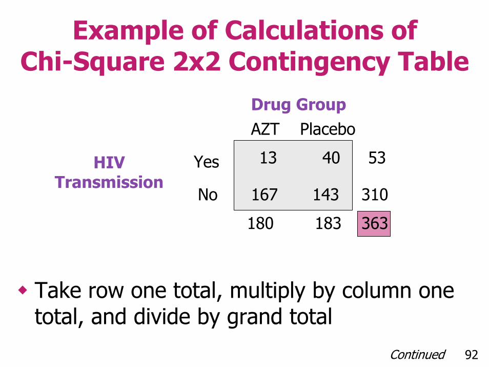
Example of Calculations of Chi-Square 2x2 Contingency Table
AZT Placebo
Yes
No
Drug Group
HIVTransmission
13 40
167 143
180 183
53
310
363
Take row one total, multiply by column one total, and divide by grand total
92Continued
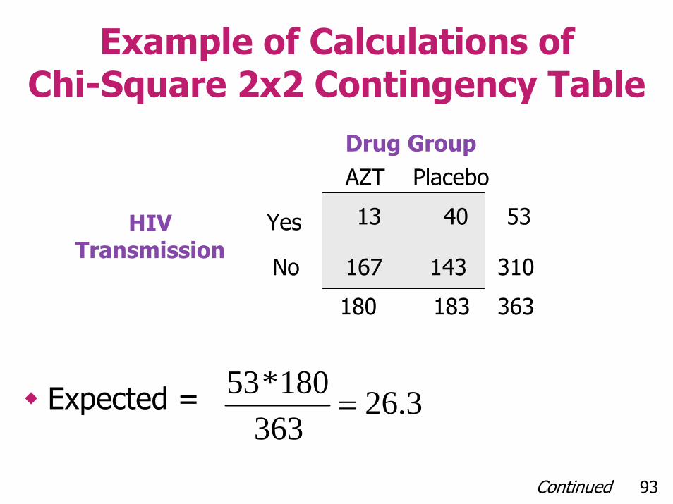
Example of Calculations of Chi-Square 2x2 Contingency Table
Expected = 3.26363
180*53=
AZT Placebo
Yes
No
Drug Group
HIVTransmission
13 40
167 143
180 183
53
310
363
93Continued

Example of Calculations of Chi-Square 2x2 Contingency Table
AZT Placebo
Yes
No
Drug Group
HIVTransmission
13 40
167 143
180 183
53
310
363
We could do the same for the other three cells; the above table has expected counts
94Continued
Example of Calculations of Chi-Square 2x2 Contingency Table
∑=χcells 4
22
EE)-(0
Test statistic
In our table 6.15= χ 2
95Continued
Sampling Distribution: Chi-Square with One Degree of Freedom
0.2
.4.6
.8P
roba
bility
0 1 5 10 15 20Chi-squared Value
96
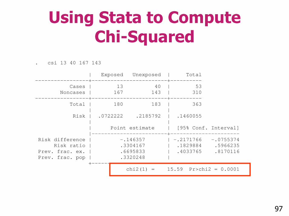
Using Stata to Compute Chi-Squared
. csi 13 40 167 143 | Exposed Unexposed | Total -----------------+------------------------+---------- Cases | 13 40 | 53 Noncases | 167 143 | 310 -----------------+------------------------+---------- Total | 180 183 | 363 | | Risk | .0722222 .2185792 | .1460055 | | | Point estimate | [95% Conf. Interval] |------------------------+---------------------- Risk difference | -.146357 | -.2171766 -.0755374 Risk ratio | .3304167 | .1829884 .5966235 Prev. frac. ex. | .6695833 | .4033765 .8170116 Prev. frac. pop | .3320248 | +----------------------------------------------- chi2(1) = 15.59 Pr>chi2 = 0.0001
97

Summary: Large Sample Procedures for Comparing Proportions Between Two
Independent PopulationsTo create a 95% confidence interval for the difference in two proportions
)ˆˆ(2ˆˆ 2121 ppSEpp −±−
98Continued
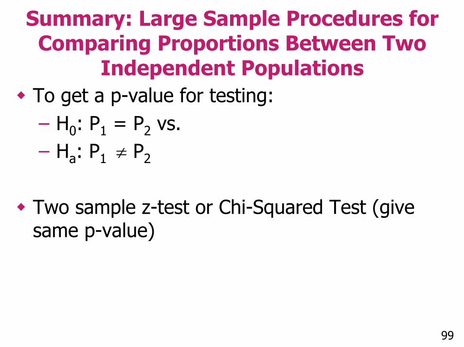
Summary: Large Sample Procedures for Comparing Proportions Between Two
Independent PopulationsTo get a p-value for testing:– H0: P1 = P2 vs.– Ha: P1 ≠ P2
Two sample z-test or Chi-Squared Test (give same p-value)
99

Extendability of Chi-Squared
Chi-squared test can be extended to test for differences in proportions across more than two independent populations– Proportion analogue to ANOVA
100
Section C
Fisher’s Exact Test
Hypothesis Testing Problem
H0: P1 = P2
Ha: P1 ≠ P2
– WhereP1 = Proportion infected on AZTP2 = Proportion infected on placebo
102Continued
Hypothesis Testing Problem
H0: P1 - P2 = 0Ha: P1 - P2 ≠ 0– Where:
P1 = Proportion infected on AZTP2 = Proportion infected on placebo
103Continued
Hypothesis Testing Problem
H0: P1 = P2
Ha: P1 ≠ P2
– In the context of the 2x2 table, this is testing whether there is a relationship between the rows (HIV status) and columns (treatment type)
104

Statistical Test Procedures
Fisher’s Exact Test– Calculations are difficult– Always appropriate to test equality of two
proportions– Computers are usually used– Exact p-value (no approximations): no
minimum sample size requirements
105Continued
Statistical Test Procedures
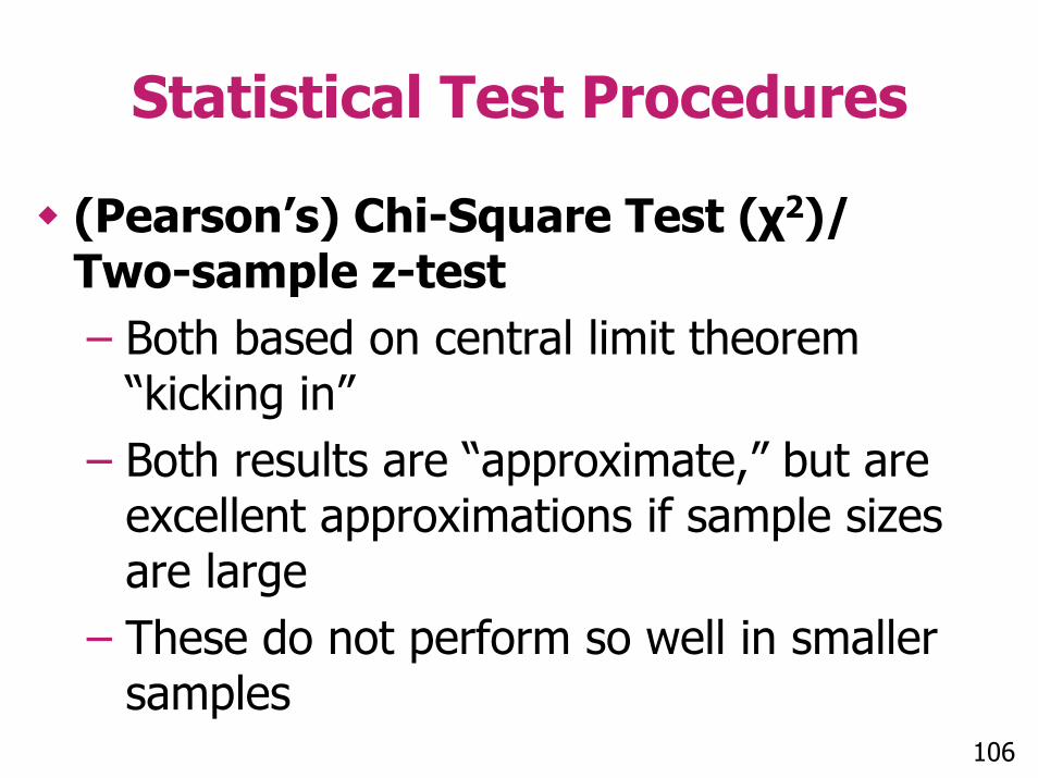
(Pearson’s) Chi-Square Test (χ2)/ Two-sample z-test– Both based on central limit theorem
“kicking in”– Both results are “approximate,” but are
excellent approximations if sample sizes are large
– These do not perform so well in smaller samples
106
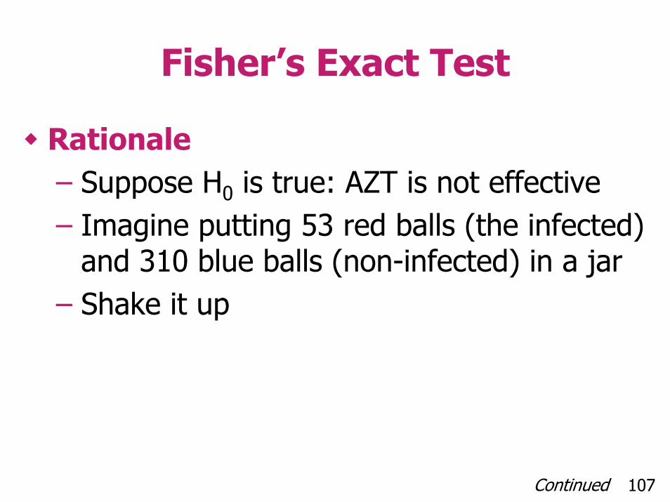
Fisher’s Exact Test
Rationale– Suppose H0 is true: AZT is not effective– Imagine putting 53 red balls (the infected)
and 310 blue balls (non-infected) in a jar– Shake it up
107Continued
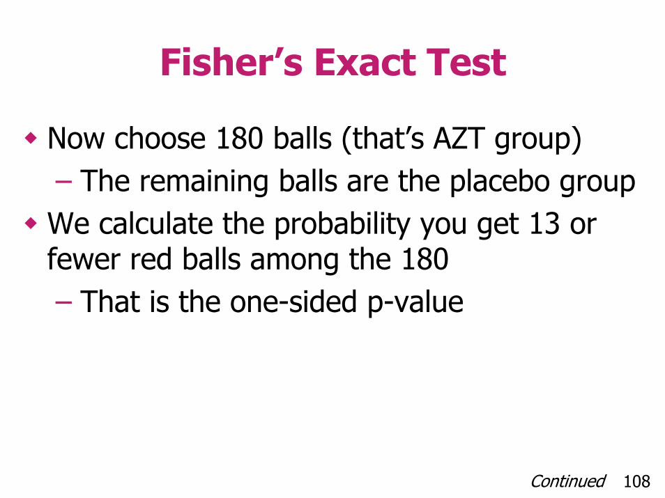
Fisher’s Exact Test
Now choose 180 balls (that’s AZT group)– The remaining balls are the placebo groupWe calculate the probability you get 13 or fewer red balls among the 180– That is the one-sided p-value
108Continued

Fisher’s Exact Test
The two-sided p-value is just about (but not exactly) twice the one-sided P-value – It accounts for the probability of getting
either extremely few red balls or a lot of red balls in the AZT group
109Continued
Fisher’s Exact Test
The p-value is the probability of obtaining a result as or more extreme (more imbalance) than you did by chance alone
110
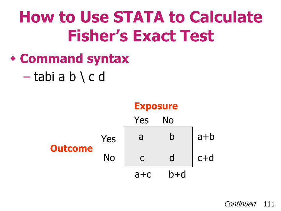
How to Use STATA to Calculate Fisher’s Exact Test
Command syntax– tabi a b \ c d
ExposureYes No
a b
c d
a+bYesOutcome
No c+d
a+c b+d
111Continued
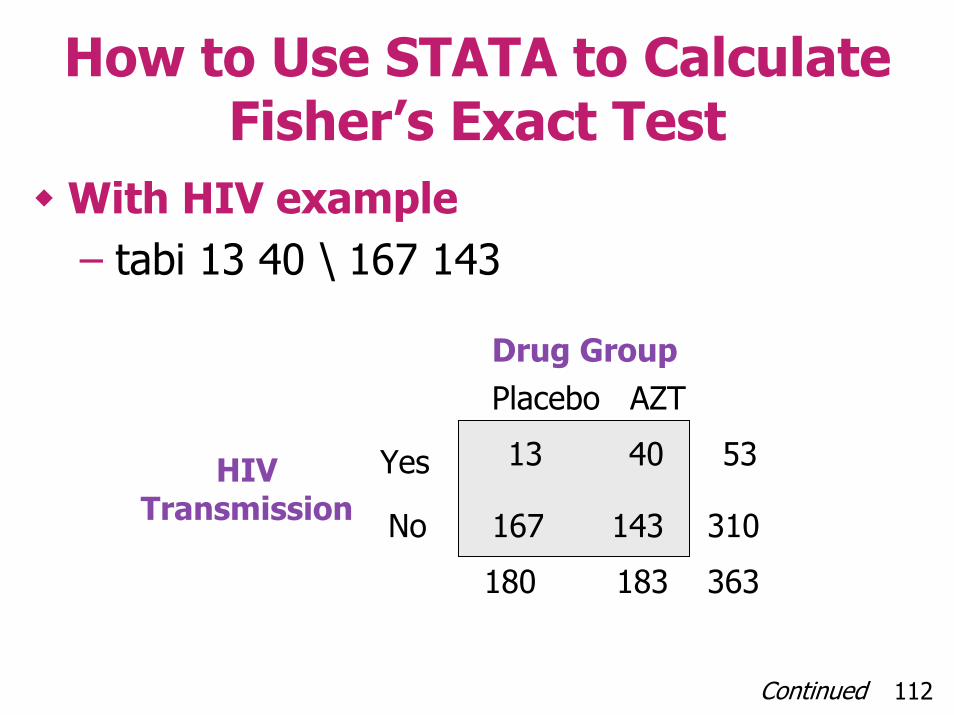
How to Use STATA to Calculate Fisher’s Exact Test
With HIV example– tabi 13 40 \ 167 143
Drug GroupPlacebo AZT
5313 40
167 143
YesHIVTransmission 310No
180 183 363
112Continued
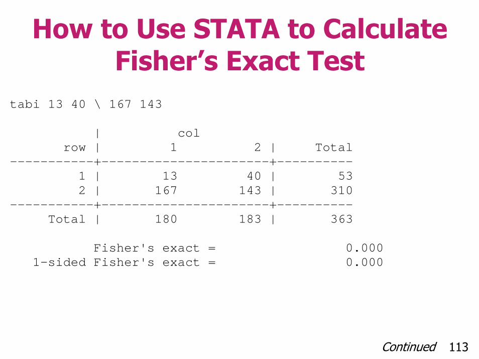
How to Use STATA to Calculate Fisher’s Exact Test
tabi 13 40 \ 167 143 | col row | 1 2 | Total -----------+----------------------+---------- 1 | 13 40 | 53 2 | 167 143 | 310 -----------+----------------------+---------- Total | 180 183 | 363 Fisher's exact = 0.000 1-sided Fisher's exact = 0.000
113Continued
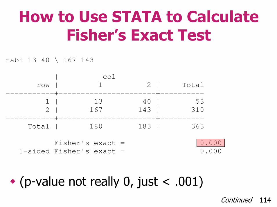
How to Use STATA to Calculate Fisher’s Exact Test
(p-value not really 0, just < .001)
tabi 13 40 \ 167 143 | col row | 1 2 | Total -----------+----------------------+---------- 1 | 13 40 | 53 2 | 167 143 | 310 -----------+----------------------+---------- Total | 180 183 | 363 Fisher's exact = 0.000 1-sided Fisher's exact = 0.000
114Continued
How to Use STATA to Calculate Fisher’s Exact Test
However, the tabi command did not give a confidence interval for the difference in proportions!Can also use csi command with “exact”option
115Continued
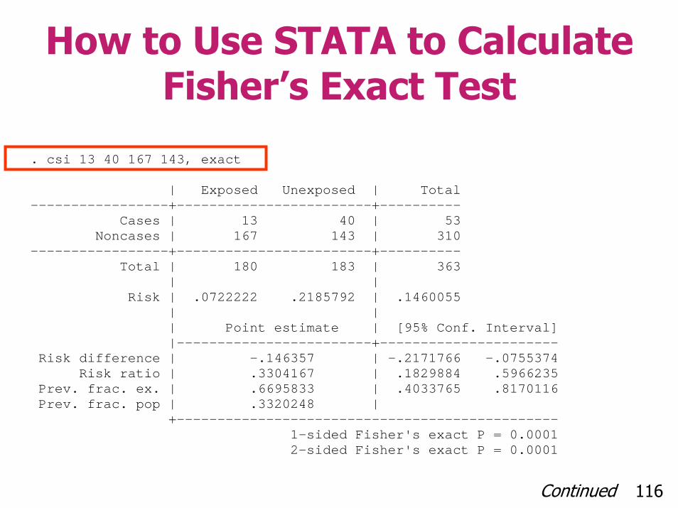
How to Use STATA to Calculate Fisher’s Exact Test
. csi 13 40 167 143, exact | Exposed Unexposed | Total -----------------+------------------------+---------- Cases | 13 40 | 53 Noncases | 167 143 | 310 -----------------+------------------------+---------- Total | 180 183 | 363 | | Risk | .0722222 .2185792 | .1460055 | | | Point estimate | [95% Conf. Interval] |------------------------+---------------------- Risk difference | -.146357 | -.2171766 -.0755374 Risk ratio | .3304167 | .1829884 .5966235 Prev. frac. ex. | .6695833 | .4033765 .8170116 Prev. frac. pop | .3320248 | +----------------------------------------------- 1-sided Fisher's exact P = 0.0001 2-sided Fisher's exact P = 0.0001
116Continued

How to Use STATA to Calculate Fisher’s Exact Test
. csi 13 40 167 143, exact | Exposed Unexposed | Total -----------------+------------------------+---------- Cases | 13 40 | 53 Noncases | 167 143 | 310 -----------------+------------------------+---------- Total | 180 183 | 363 | | Risk | .0722222 .2185792 | .1460055 | | | Point estimate | [95% Conf. Interval] |------------------------+---------------------- Risk difference | -.146357 | -.2171766 -.0755374 Risk ratio | .3304167 | .1829884 .5966235 Prev. frac. ex. | .6695833 | .4033765 .8170116 Prev. frac. pop | .3320248 | +----------------------------------------------- 1-sided Fisher's exact P = 0.0001 2-sided Fisher's exact P = 0.0001
117Continued
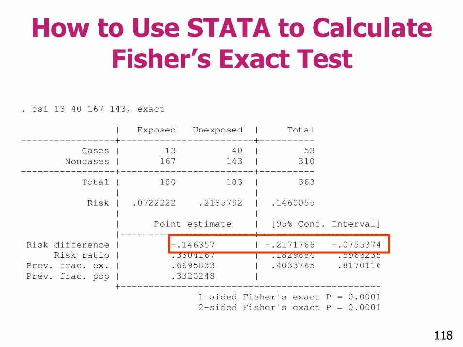
How to Use STATA to Calculate Fisher’s Exact Test
. csi 13 40 167 143, exact | Exposed Unexposed | Total -----------------+------------------------+---------- Cases | 13 40 | 53 Noncases | 167 143 | 310 -----------------+------------------------+---------- Total | 180 183 | 363 | | Risk | .0722222 .2185792 | .1460055 | | | Point estimate | [95% Conf. Interval] |------------------------+---------------------- Risk difference | -.146357 | -.2171766 -.0755374 Risk ratio | .3304167 | .1829884 .5966235 Prev. frac. ex. | .6695833 | .4033765 .8170116 Prev. frac. pop | .3320248 | +----------------------------------------------- 1-sided Fisher's exact P = 0.0001 2-sided Fisher's exact P = 0.0001
118
Small Sample Application
Sixty-five pregnant women, all who were classified as having a high risk of pregnancy induced hypertension, were recruited to participate in a study of the effects of aspirin on hypertensionThe women were randomized to receive either 100 mg of aspirin daily, or a placebo during the third trimester of pregnancy
1. Schiff, E. et al; The use of aspirin to prevent pregnancy-induced hypertension and lower the ratio of thromboxane A2 to prostacyclinin relatively high risk pregnancies, New England Journal of Medicine321;6 119Continued
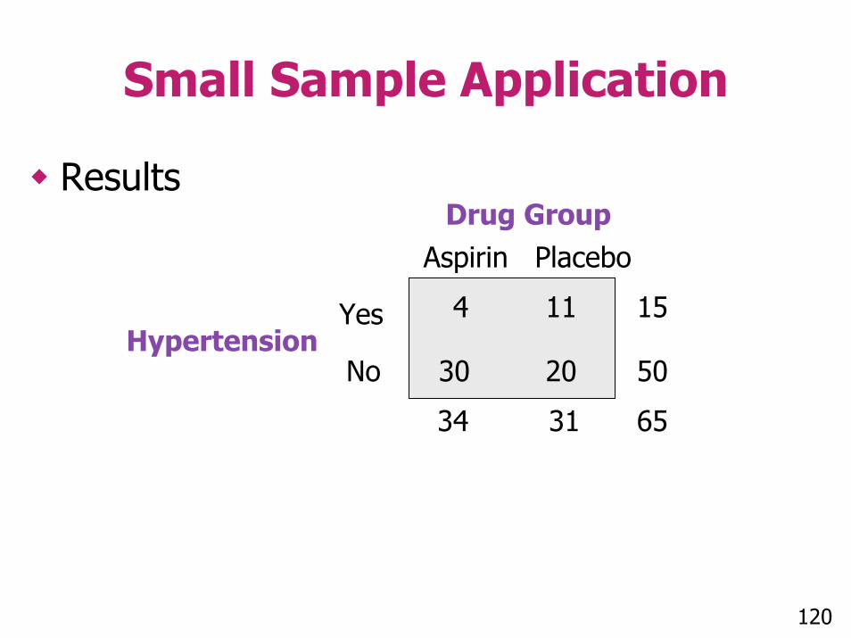
Small Sample Application
ResultsDrug Group
Aspirin Placebo
4 11
30 20
15YesHypertension
No 50
34 31 65
120

Sample Proportions
35.3111ˆ
12.344ˆ
==
==
placebo
aspirin
p
p
121
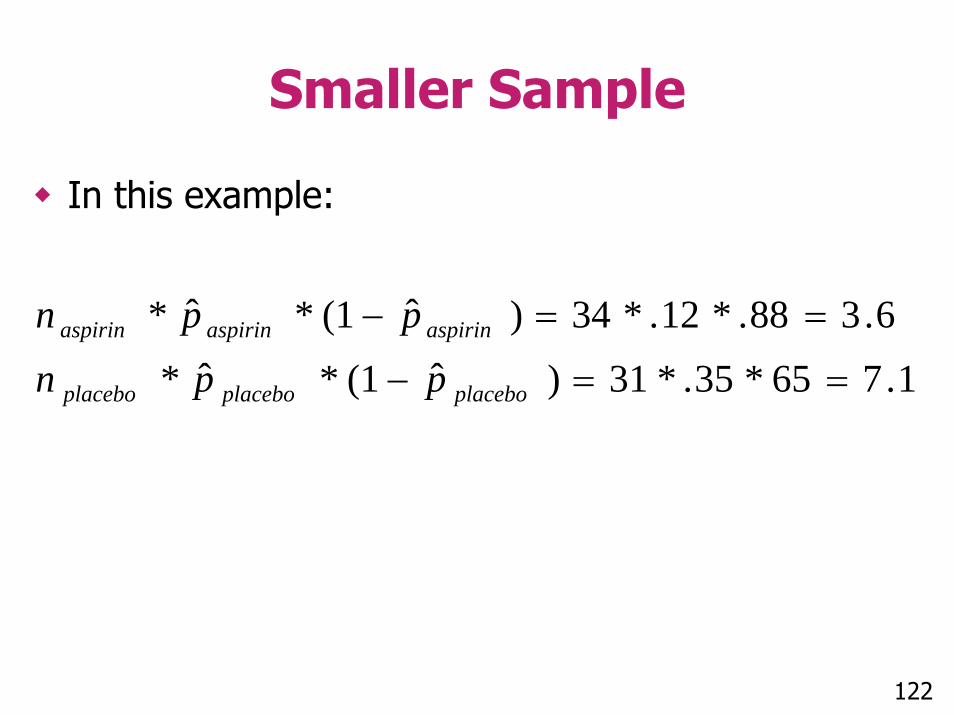
Smaller Sample
In this example:
1.765*35.*31)ˆ1(*ˆ*6.388.*12.*34)ˆ1(*ˆ*
==−
==−
placeboplaceboplacebo
aspirinaspirinaspirin
ppnppn
122
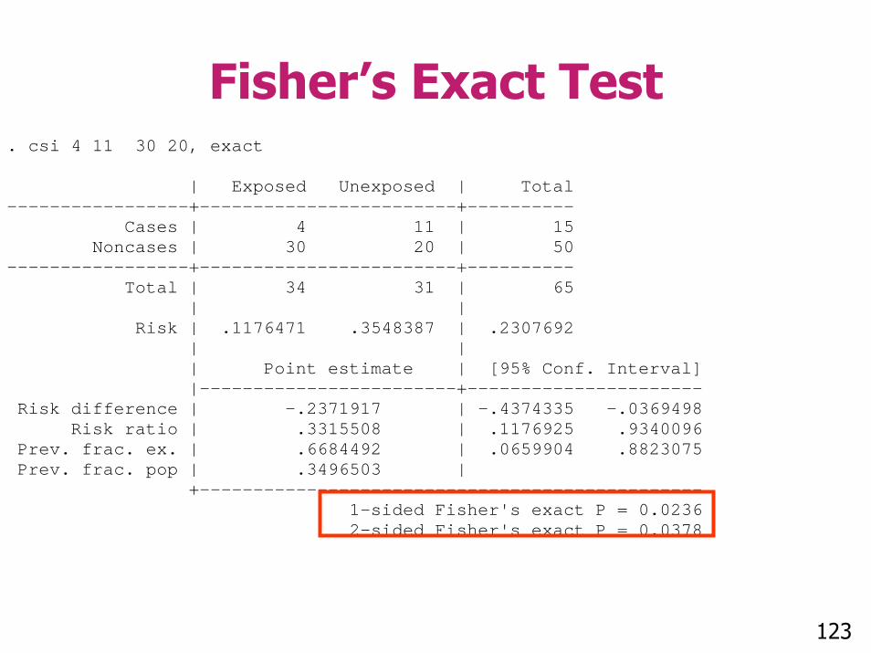
Fisher’s Exact Test. csi 4 11 30 20, exact | Exposed Unexposed | Total -----------------+------------------------+---------- Cases | 4 11 | 15 Noncases | 30 20 | 50 -----------------+------------------------+---------- Total | 34 31 | 65 | | Risk | .1176471 .3548387 | .2307692 | | | Point estimate | [95% Conf. Interval] |------------------------+---------------------- Risk difference | -.2371917 | -.4374335 -.0369498 Risk ratio | .3315508 | .1176925 .9340096 Prev. frac. ex. | .6684492 | .0659904 .8823075 Prev. frac. pop | .3496503 | +----------------------------------------------- 1-sided Fisher's exact P = 0.0236 2-sided Fisher's exact P = 0.0378
123
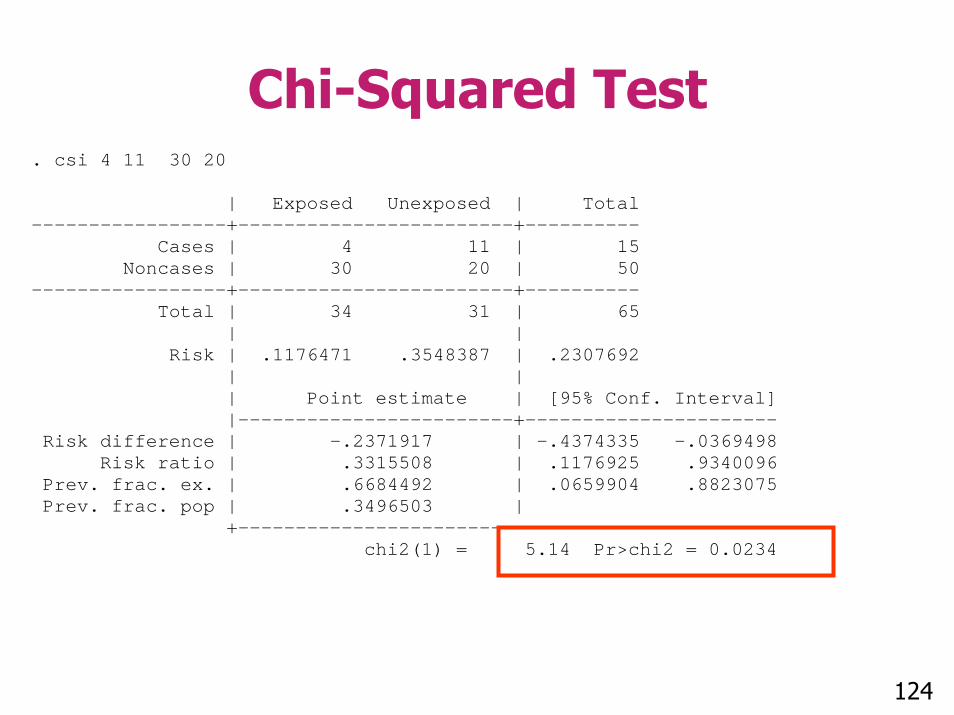
Chi-Squared Test. csi 4 11 30 20 | Exposed Unexposed | Total -----------------+------------------------+---------- Cases | 4 11 | 15 Noncases | 30 20 | 50 -----------------+------------------------+---------- Total | 34 31 | 65 | | Risk | .1176471 .3548387 | .2307692 | | | Point estimate | [95% Conf. Interval] |------------------------+---------------------- Risk difference | -.2371917 | -.4374335 -.0369498 Risk ratio | .3315508 | .1176925 .9340096 Prev. frac. ex. | .6684492 | .0659904 .8823075 Prev. frac. pop | .3496503 | +----------------------------------------------- chi2(1) = 5.14 Pr>chi2 = 0.0234
124
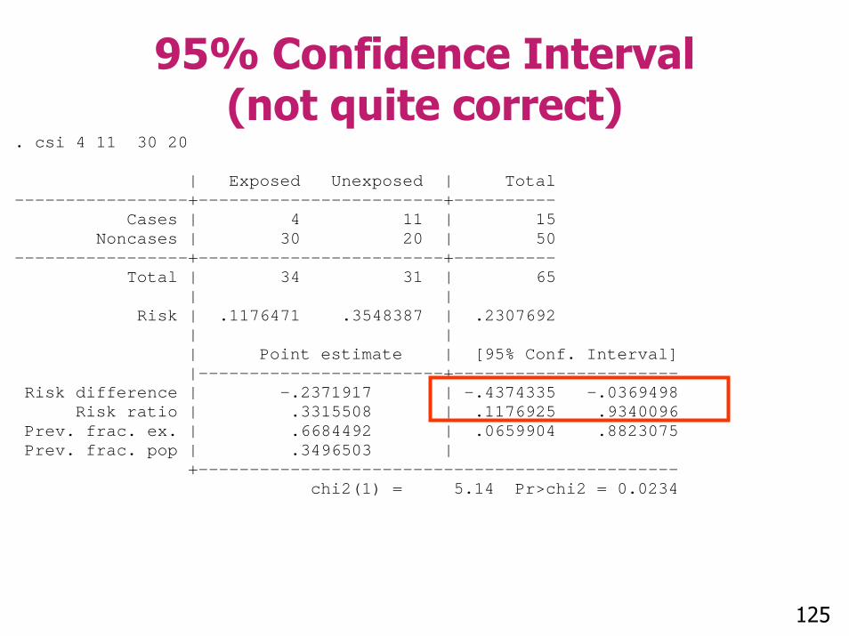
95% Confidence Interval (not quite correct)
. csi 4 11 30 20 | Exposed Unexposed | Total -----------------+------------------------+---------- Cases | 4 11 | 15 Noncases | 30 20 | 50 -----------------+------------------------+---------- Total | 34 31 | 65 | | Risk | .1176471 .3548387 | .2307692 | | | Point estimate | [95% Conf. Interval] |------------------------+---------------------- Risk difference | -.2371917 | -.4374335 -.0369498 Risk ratio | .3315508 | .1176925 .9340096 Prev. frac. ex. | .6684492 | .0659904 .8823075 Prev. frac. pop | .3496503 | +----------------------------------------------- chi2(1) = 5.14 Pr>chi2 = 0.0234
125
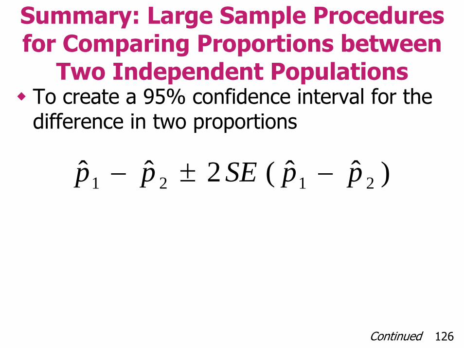
Summary: Large Sample Procedures for Comparing Proportions between
Two Independent PopulationsTo create a 95% confidence interval for the difference in two proportions
)ˆˆ(2ˆˆ 2121 ppSEpp −±−
126Continued
Summary: Large Sample Procedures for Comparing Proportions Between Two
Independent PopulationsTo get a p-value for testing:– H0: P1 = P2 vs.– Ha: P1 ≠ P2
Two Sample z-test or Chi-Squared Test (give same p-value)Fisher’s exact
127

Small Sample Procedures for Comparing Proportions Between Two Independent
PopulationsTo create a 95% confidence interval for the difference in two proportions, can use this result as a guideline:
Not quite correct but will give you a good sense of width/range of CI
)ˆˆ(2ˆˆ 2121 ppSEpp −±−
128
Summary: Large Sample Procedures for Comparing Proportions Between Two
Independent PopulationsTo get a p-value for testing:– H0: P1 = P2 vs.– Ha: P1 ≠ P2
Fisher’s exact test
129

Section C
Practice Problems

Practice Problems
Researchers are interested in studying the relationship between salt in a diet and high blood pressure in men in their early 50s A random sample is taken of 58 men between the ages of 50–54Each subject keeps a food diary for a one-month period, and is evaluated for high blood pressure
Continued 131

Practice Problems
Seven of the 58 men have high salt diets– Of these seven men, one had high blood
pressure at the time of the study51 of the 58 men have low salt diets– Of these 58 men, 28 have high blood
pressure at the time of the study
Continued 132
Practice Problems
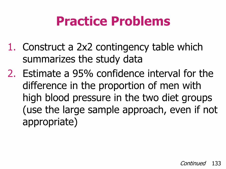
1. Construct a 2x2 contingency table which summarizes the study data
2. Estimate a 95% confidence interval for the difference in the proportion of men with high blood pressure in the two diet groups (use the large sample approach, even if not appropriate)
Continued 133

Practice Problems
3. Perform (using computer) both a Fisher’s exact test and a chi-squared test
– If you were using a strict .05 level cutoff for statistical significance, how would your conclusions from each of the two tests compare?
134

Section C
Practice Problem Solutions
Practice Problems
Researchers are interested in studying the relationship between salt in a diet and high blood pressure in men in their early 50s A random sample is taken of 58 men between the ages of 50–54Each subject keeps a food diary for a one-month period and is evaluated for high blood pressure
Continued 136
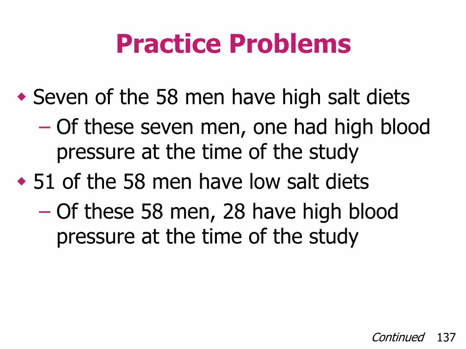
Practice Problems
Seven of the 58 men have high salt diets– Of these seven men, one had high blood
pressure at the time of the study51 of the 58 men have low salt diets– Of these 58 men, 28 have high blood
pressure at the time of the study
Continued 137
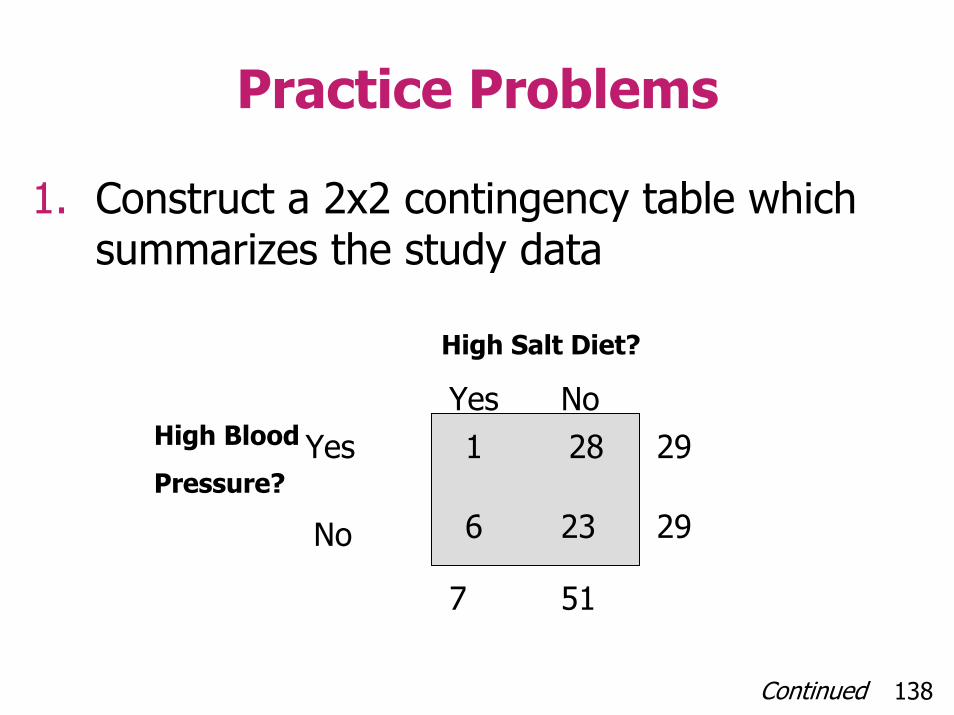
Practice Problems
1. Construct a 2x2 contingency table which summarizes the study data
Yes
No
High Salt Diet?
Yes No1
6
28
23
29
29
7 51
High Blood
Pressure?
Continued 138
Practice Problems
2. Estimate a 95% confidence interval for the difference in the proportion of men with high blood pressure in the two diet groups (use the large sample approach, even if not appropriate)
Continued 139
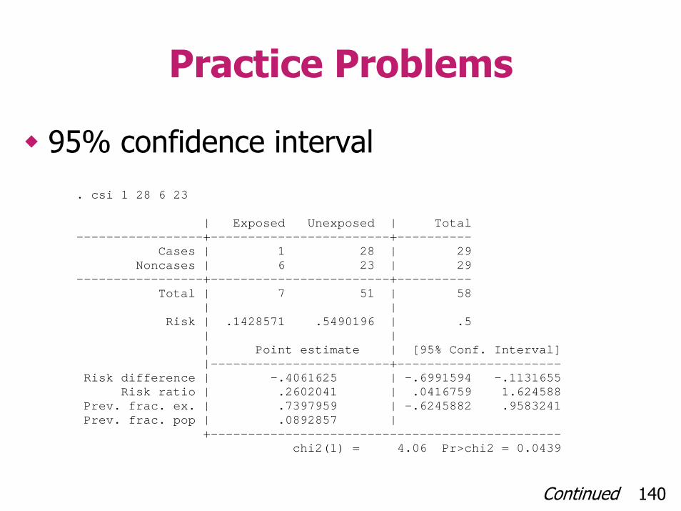
Practice Problems
95% confidence interval. csi 1 28 6 23 | Exposed Unexposed | Total -----------------+------------------------+---------- Cases | 1 28 | 29 Noncases | 6 23 | 29 -----------------+------------------------+---------- Total | 7 51 | 58 | | Risk | .1428571 .5490196 | .5 | | | Point estimate | [95% Conf. Interval] |------------------------+---------------------- Risk difference | -.4061625 | -.6991594 -.1131655 Risk ratio | .2602041 | .0416759 1.624588 Prev. frac. ex. | .7397959 | -.6245882 .9583241 Prev. frac. pop | .0892857 | +----------------------------------------------- chi2(1) = 4.06 Pr>chi2 = 0.0439
Continued 140
Practice Problems
3. Perform (using computer) both a Fisher’s exact test and a chi-squared test
– If you were using a strict .05 level cutoff for statistical significances, how would your conclusions from each of the two tests compare?
Continued 141
Practice Problems
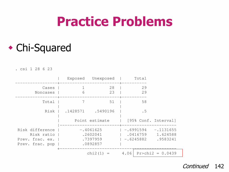
Chi-Squared
. csi 1 28 6 23 | Exposed Unexposed | Total -----------------+------------------------+---------- Cases | 1 28 | 29 Noncases | 6 23 | 29 -----------------+------------------------+---------- Total | 7 51 | 58 | | Risk | .1428571 .5490196 | .5 | | | Point estimate | [95% Conf. Interval] |------------------------+---------------------- Risk difference | -.4061625 | -.6991594 -.1131655 Risk ratio | .2602041 | .0416759 1.624588 Prev. frac. ex. | .7397959 | -.6245882 .9583241 Prev. frac. pop | .0892857 | +----------------------------------------------- chi2(1) = 4.06 Pr>chi2 = 0.0439
Continued 142

Practice Problems
Fisher’s Exact
. csi 1 28 6 23, exact | Exposed Unexposed | Total -----------------+------------------------+---------- Cases | 1 28 | 29 Noncases | 6 23 | 29 -----------------+------------------------+---------- Total | 7 51 | 58 | | Risk | .1428571 .5490196 | .5 | | | Point estimate | [95% Conf. Interval] |------------------------+---------------------- Risk difference | -.4061625 | -.6991594 -.1131655 Risk ratio | .2602041 | .0416759 1.624588 Prev. frac. ex. | .7397959 | -.6245882 .9583241 Prev. frac. pop | .0892857 | +----------------------------------------------- 1-sided Fisher's exact P = 0.0510 2-sided Fisher's exact P = 0.1020
143
Section D
Measures of Association: Risk Difference, Relative Risk and
the Odds Ratio
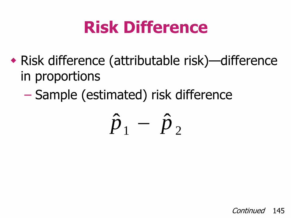
Risk Difference
Risk difference (attributable risk)—difference in proportions– Sample (estimated) risk difference
21 ˆˆ pp −
145Continued

Risk Difference
The difference in risk of HIV for children born to HIV+ mothers taking AZT relative to HIV+ mothers taking placebo
15.22.07.ˆˆ 21 −=−=− pp
146Continued
Risk Difference
Interpretation– If AZT was given to 1,000 HIV infected
pregnant women, this would reduce the number of HIV positive infants by 150 relative the number of HIV positive infants born to 1,000 women not treated with AZT
147Continued

Risk Difference. csi 13 40 167 143 | Exposed Unexposed | Total -----------------+------------------------+---------- Cases | 13 40 | 53 Noncases | 167 143 | 310 -----------------+------------------------+---------- Total | 180 183 | 363 | | Risk | .0722222 .2185792 | .1460055 | | | Point estimate | [95% Conf. Interval] |------------------------+---------------------- Risk difference | -.146357 | -.2171766 -.0755374 Risk ratio | .3304167 | .1829884 .5966235 Prev. frac. ex. | .6695833 | .4033765 .8170116 Prev. frac. pop | .3320248 | +----------------------------------------------- chi2(1) = 15.59 Pr>chi2 = 0.0001
148Continued

Risk Difference
Interpretation– Study results suggest that the reduction in
HIV positive births from 1,000 HIV positive pregnant women treated with AZT could range from 75 to 220 fewer than the number occurring if the 1,000 women were not treated
149
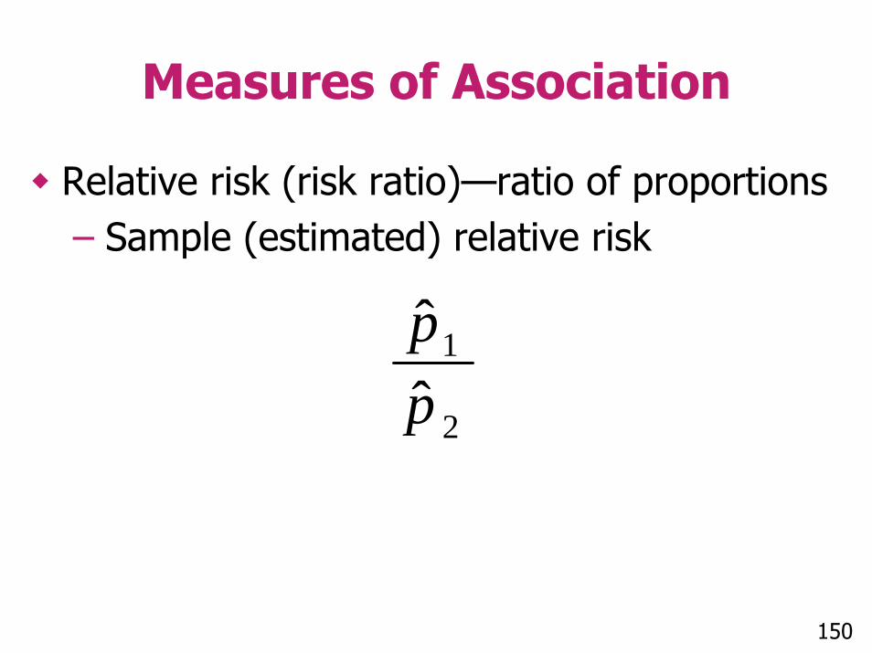
Measures of Association
Relative risk (risk ratio)—ratio of proportions– Sample (estimated) relative risk
2
1
ˆˆpp
150
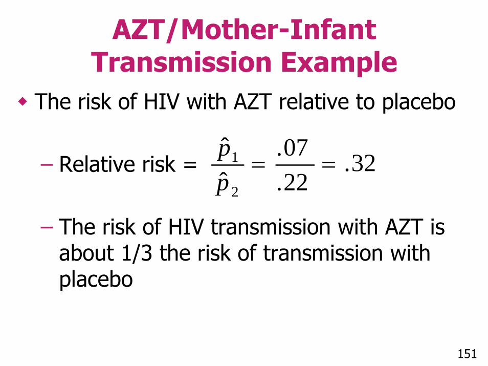
AZT/Mother-Infant Transmission Example
The risk of HIV with AZT relative to placebo
– Relative risk =
– The risk of HIV transmission with AZT is about 1/3 the risk of transmission with placebo
32.22.07.
ˆˆ
2
1 ==pp
151
Relative Risk
Interpretation– An HIV positive pregnant woman could
reduce her personal risk of giving birth to an HIV positive child by nearly 70% if she takes AZT during her pregnancy
152Continued
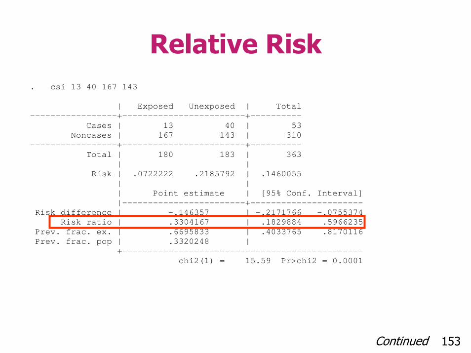
Relative Risk. csi 13 40 167 143 | Exposed Unexposed | Total -----------------+------------------------+---------- Cases | 13 40 | 53 Noncases | 167 143 | 310 -----------------+------------------------+---------- Total | 180 183 | 363 | | Risk | .0722222 .2185792 | .1460055 | | | Point estimate | [95% Conf. Interval] |------------------------+---------------------- Risk difference | -.146357 | -.2171766 -.0755374 Risk ratio | .3304167 | .1829884 .5966235 Prev. frac. ex. | .6695833 | .4033765 .8170116 Prev. frac. pop | .3320248 | +----------------------------------------------- chi2(1) = 15.59 Pr>chi2 = 0.0001
153Continued
Relative Risk
Interpretation– Study results suggest that this reduction in
risk could be as small as 40% and as large as 82%
154
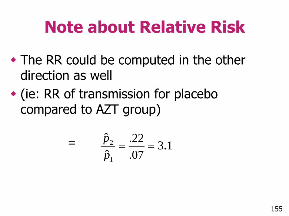
Note about Relative Risk
The RR could be computed in the other direction as well(ie: RR of transmission for placebo compared to AZT group)
= 1.307.22.
ˆˆ
1
2 ==pp
155

Relative Risk
Interpretation– An HIV positive pregnant woman
increases her personal risk of giving birth to an HIV positive child by slightly more than 3 times if she does not take AZT during her pregnancy
156Continued

Relative Risk. csi 40 13 143 167 | Exposed Unexposed | Total -----------------+------------------------+---------- Cases | 40 13 | 53 Noncases | 143 167 | 310 -----------------+------------------------+---------- Total | 183 180 | 363 | | Risk | .2185792 .0722222 | .1460055 | | | Point estimate | [95% Conf. Interval] |------------------------+---------------------- Risk difference | .146357 | .0755374 .2171766 Risk ratio | 3.026482 | 1.676099 5.464827 Attr. frac. ex. | .6695833 | .4033765 .8170116 Attr. frac. pop | .5053459 | +----------------------------------------------- chi2(1) = 15.59 Pr>chi2 = 0.0001
157Continued
Relative Risk
Interpretation– Study results suggest that this increase in
risk could be as small as 1.7 times and as large as 5.5 times
158
Relative Risk
Direction of comparison is somewhat arbitraryDoes not affect results as long as interpreted correctly!!
159
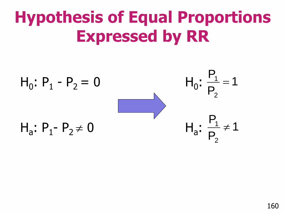
Hypothesis of Equal Proportions Expressed by RR
H0: P1 - P2 = 0 H0:
Ha: P1- P2 ≠ 0 Ha:
1PP
2
1 =
1PP
2
1 ≠
160
The Risk Difference vs. Relative Risk
The risk difference (attributable) risk provides a measure of the public health impact of an exposure (assuming causality)The relative risk provides a measure of the magnitude of the disease-exposure association for an individual
161Continued
The Risk Difference vs. Relative Risk
AZT example—in this study 22% of the untreated mothers gave birth to children with HIV– Relative Risk : .32– Risk Difference : -15%
162Continued
The Risk Difference vs. Relative Risk
Suppose that only 2% of the children born to untreated HIV positive women became HIV positiveSuppose the percentage in AZT treated women is .6%– Relative Risk : .32– Risk Difference : -1.4 %
163Continued
The Risk Difference vs. Relative Risk
Suppose that 90% of the children born to untreated HIV positive women became HIV positiveSuppose this percentage was 75% for mothers taking AZT treatment during pregnancy – Risk Difference : 15%– Relative Risk : .83
164

The Odds Ratio
Like the relative risk, the odds ratio provides a measure of association in a ratio (as opposed to difference)
165

What is an Odds?
Odds is a function of risk (prevalence).Odds is the ratio of risk of having an outcome to risk of not having an outcome.– If p represents risk of an outcome,
then the odds is given by:
ppOdds−
=1
166
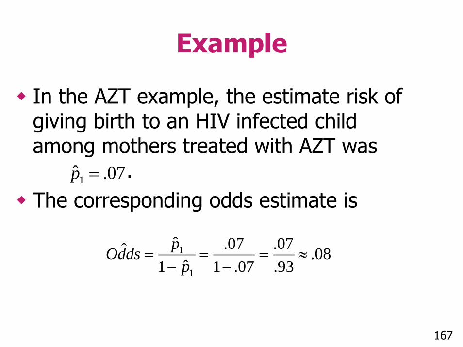
Example
In the AZT example, the estimate risk of giving birth to an HIV infected child among mothers treated with AZT was
. The corresponding odds estimate is
07.ˆ1 =p
08.93.07.
07.107.
ˆ1ˆˆ
1
1 ≈=−
=−
=p
pdsdO
167
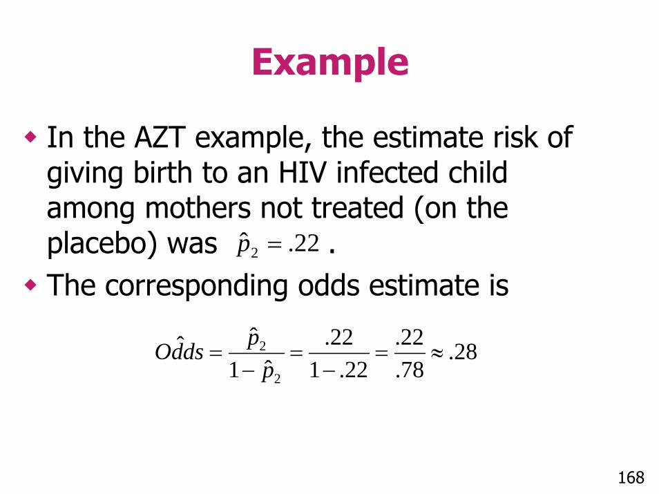
Example
In the AZT example, the estimate risk of giving birth to an HIV infected child among mothers not treated (on the placebo) was . The corresponding odds estimate is
22.ˆ 2 =p
28.78.22.
22.122.
ˆ1ˆˆ
2
2 ≈=−
=−
=p
pdsdO
168
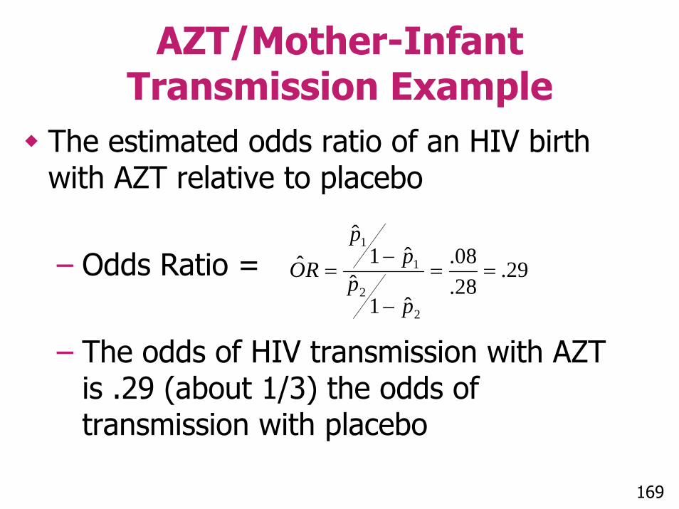
AZT/Mother-Infant Transmission Example
The estimated odds ratio of an HIV birth with AZT relative to placebo
– Odds Ratio =
– The odds of HIV transmission with AZT is .29 (about 1/3) the odds of transmission with placebo
29.28.08.
ˆ1ˆ
ˆ1ˆ
ˆ
2
2
1
1
==
−
−=
pp
pp
RO
169

Estimating Odds Ratio With Stata
. csi 13 40 167 143, or | Exposed Unexposed | Total -----------------+------------------------+---------- Cases | 13 40 | 53 Noncases | 167 143 | 310 -----------------+------------------------+---------- Total | 180 183 | 363 | | Risk | .0722222 .2185792 | .1460055 | | | Point estimate | [95% Conf. Interval] |------------------------+---------------------- Risk difference | -.146357 | -.2171766 -.0755374 Risk ratio | .3304167 | .1829884 .5966235 Prev. frac. ex. | .6695833 | .4033765 .8170116 Prev. frac. pop | .3320248 | Odds ratio | .2782934 | .1445784 .5363045 (Cornfield) +----------------------------------------------- chi2(1) = 15.59 Pr>chi2 = 0.0001
170
Odds Ratio
Interpretation– AZT is associated with an estimated 71%
(estimated OR = .29) reduction in odds of giving birth to an HIV infected child among HIV infected pregnant women
– Study results suggest that this reduction in odds could be as small as 46% and as large as 86% (95% CI on odds ratio, .14-.54)
171Continued
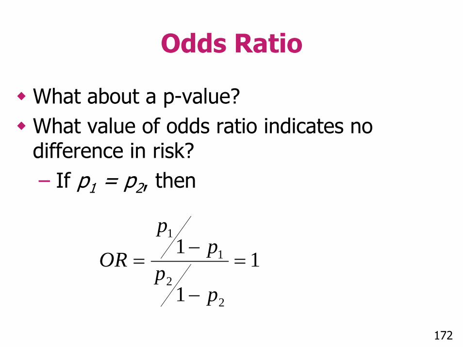
Odds Ratio
What about a p-value?What value of odds ratio indicates no difference in risk?– If p1 = p2, then
1
1
1
2
2
1
1
=
−
−=
pp
pp
OR
172
Odds Ratio
Hence we need to testHo: OR=1
vs. Ha: OR ≠1
But, from previous slide OR = 1 only if p1=p2: so same test from before applies!
173
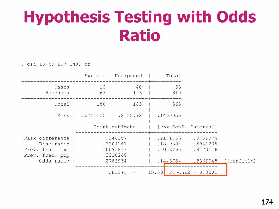
Hypothesis Testing with Odds Ratio
. csi 13 40 167 143, or | Exposed Unexposed | Total -----------------+------------------------+---------- Cases | 13 40 | 53 Noncases | 167 143 | 310 -----------------+------------------------+---------- Total | 180 183 | 363 | | Risk | .0722222 .2185792 | .1460055 | | | Point estimate | [95% Conf. Interval] |------------------------+---------------------- Risk difference | -.146357 | -.2171766 -.0755374 Risk ratio | .3304167 | .1829884 .5966235 Prev. frac. ex. | .6695833 | .4033765 .8170116 Prev. frac. pop | .3320248 | Odds ratio | .2782934 | .1445784 .5363045 (Cornfield) +----------------------------------------------- chi2(1) = 15.59 Pr>chi2 = 0.0001
174

Hypothesis of Equal Proportions Expressed by RR or OR
H0: P1 - P2 = 0 H0: RR=1 H0: OR=1
Ha: P1- P2 ≠ 0 Ha: RR=1 Ha: OR ≠1
175
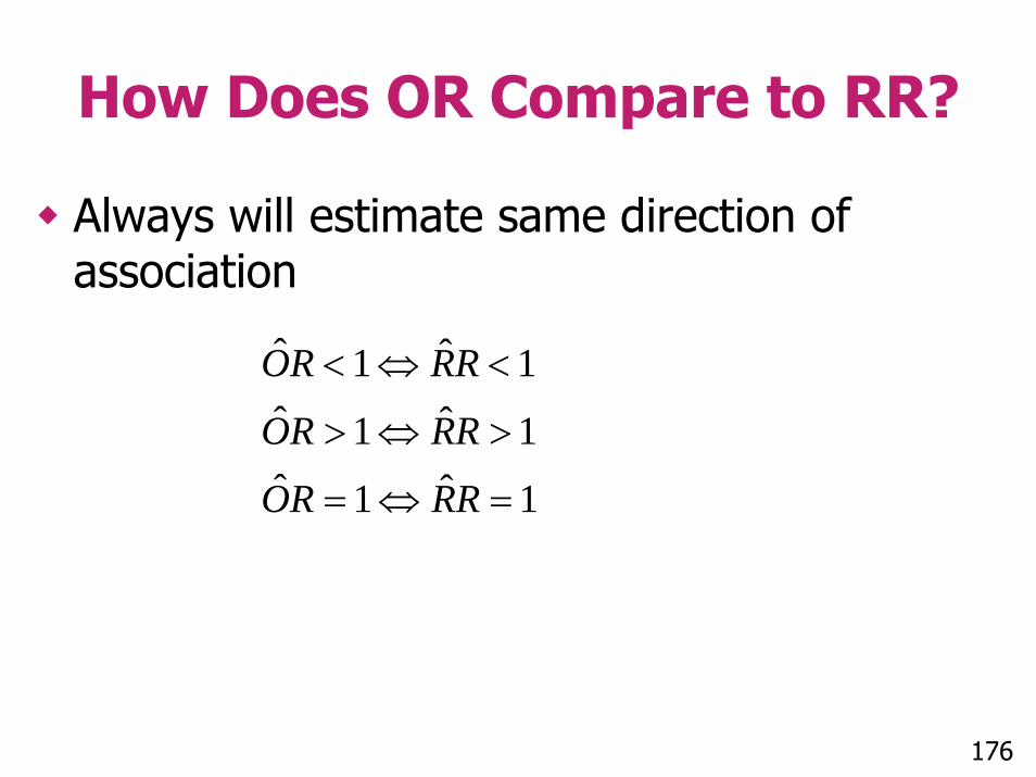
How Does OR Compare to RR?
Always will estimate same direction of association
1ˆ1ˆ1ˆ1ˆ1ˆ1ˆ
=⇔=
>⇔>
<⇔<
RRRO
RRRO
RRRO
176

How Does OR Compare to RR?
If CI for OR does not include 1, CI for RR will not include 1If CI for OR includes 1, CI for RR will include 1
111111
=⇔=>⇔><⇔<
RRORRRORRROR
177
How Does OR Compare to RR?
The lower the risk in both groups being compared, the more similar the OR and RRwill be in magnitude
178

The Odds Ratiovs. Relative Risk
AZT example—in this study 7% of AZT treated mothers and 22% of the untreated mothers gave birth to children with HIV– Relative Risk : .32– Odds Ratio : .28
179Continued

The Risk Difference vs. Relative Risk
Suppose that only 2% of the children born to untreated HIV positive women became HIV positiveSuppose the percentage in AZT treated women is .6%– Relative Risk : .32– Odds Ratio : .30
180Continued
The Risk Difference vs. Relative Risk
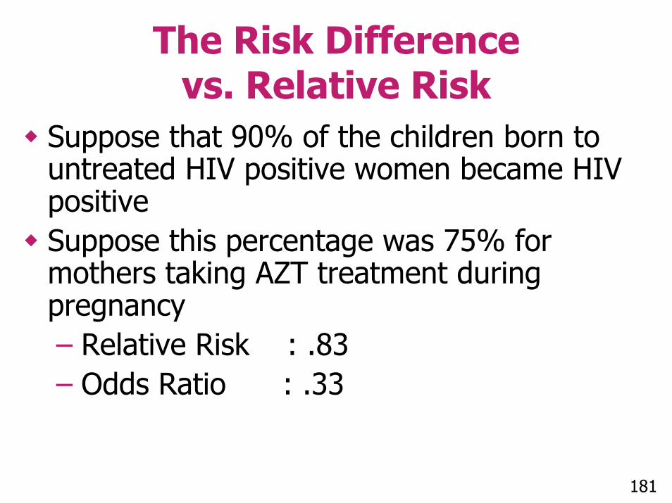
Suppose that 90% of the children born to untreated HIV positive women became HIV positiveSuppose this percentage was 75% for mothers taking AZT treatment during pregnancy – Relative Risk : .83– Odds Ratio : .33
181
Why Even Bother With Odds Ratio?
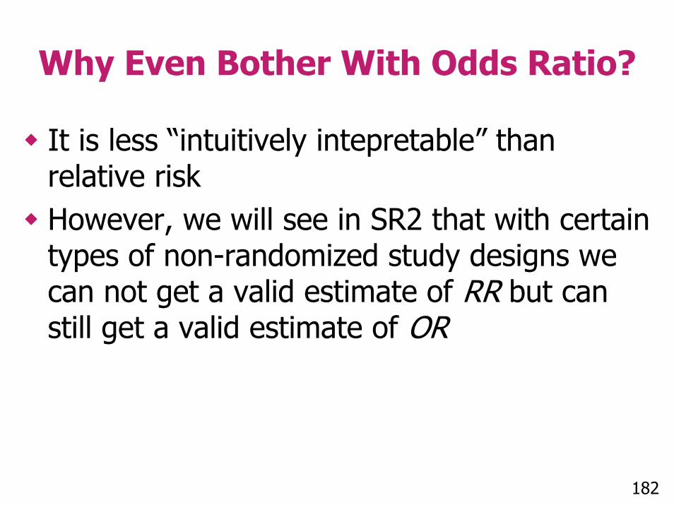
It is less “intuitively intepretable” than relative riskHowever, we will see in SR2 that with certain types of non-randomized study designs we can not get a valid estimate of RR but can still get a valid estimate of OR
182
Section D
Practice Problems
Practice Problems
1. Define relative risk for an outcome when comparing two groups. Why is the p-value for testing the equality of the proportion of subjects with the outcome across the two groups equivalent to the p-value for testing:
Ho: RR = 1vs. Ha: RR ≠ 1,
Where RR = relative risk?Continued 184
Practice Problems
2. What can one conclude about the 95% confidence interval for a relative risk if the p-value for the test described in question one is less than .05?
Continued 185
Practice Problems
186
3. In the maternal HIV transmission example, the relative risk of transmission for mothers on AZT as compared with mothers on placebo is about .30. This estimate was statistically and significantly different than one. How can this estimate be interpreted scientifically? What would the estimate be for the relative risk of transmission for mothers on placebo as compared to mothers on AZT?
Continued
Practice Problems
4. What is the relationship between a relative risk and an odds ratio? Why do we even bother with odds ratios?
Continued 187
Practice Problems
188
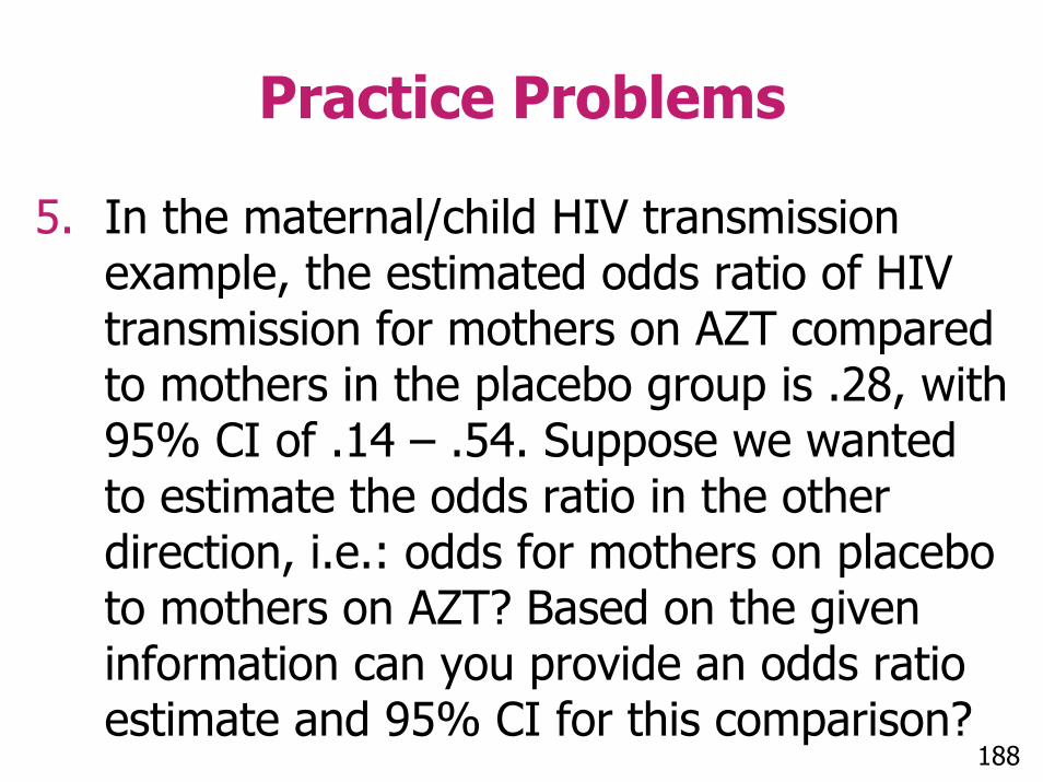
5. In the maternal/child HIV transmission example, the estimated odds ratio of HIV transmission for mothers on AZT compared to mothers in the placebo group is .28, with 95% CI of .14 – .54. Suppose we wanted to estimate the odds ratio in the other direction, i.e.: odds for mothers on placebo to mothers on AZT? Based on the given information can you provide an odds ratio estimate and 95% CI for this comparison?
Section D
Practice Problem Solutions
Question
1. Define relative risk for an outcome when comparing two groups. Why is the p-value for testing the equality of the proportion of subjects with the outcome across the two groups equivalent to the p-value for testing:
Ho: RR = 1vs. Ha: RR ≠ 1,
Where RR = relative risk?190
Answer
The relative risk is P1/P2, where P1 = proportion of subjects in group one with the outcome and P2 = proportion of subjects in group two with the outcome.This ratio, the relative risk, would be statistically different than one if P1 is statistically different from P2.Therefore, testing the equality of P1 and P2 is equivalent to testing RR =1.
Continued 191
Answer
2. What can one conclude about the 95% confidence interval for a relative risk, if the p-value for the test described in question one is less than .05?– 95% CI would not include one.
192
Question
193
3. In the maternal HIV transmission example, the relative risk of transmission for mothers on AZT as compared with mothers on placebo is about .30. This estimate was statistically and significantly different than one. How can this estimate be interpreted scientifically? What would the estimate be for the relative risk of transmission for mothers on placebo as compared to mothers on AZT?
Answer
A relative risk of .30 indicates that in this sample, mothers on AZT have .30 times the risk of transmission that mothers on placebo have (30% of the risk)Because this number is statistically significant (different than one), researchers could conclude that mothers on AZT have less risk of transmitting the virus to their children
Continued 194
Answer
195
If, instead, the relative risk of transmission for mothers on placebo, as compared to mothers on AZT was computed, this estimate would be 3.3, indicating that mother’s on placebo have over three times the risk of transmission as compared to mothers on AZTThis can be easily computed by taking the reciprocal of .30 (1/.30 = 3.3)The p-value for testing the significance of this estimate would be exactly the same as computing the relative risk in the other direction
Question
4. What is the relationship between a relative risk and an odds ratio? Why do we even bother with odds ratios?
196

Answer
The relative risk and odds ratio both provide a measure of association between an outcome and a predictor: the two measures will always concur on the direction and statistical significance of the association, but the estimates and confidence limits of the two may differ.
Continued 197
Answer
While odds ratio are less easily interpreted than relative risk, they can be estimated in situations where a valid estimate of the relative risk cannot be obtained. This will be explored further in 612.
198

Question
199
5. In the maternal/child HIV transmission example, the estimated odds ratio of HIV transmission for mothers on AZT compared to mothers in the placebo group is .28, with 95% CI of .15 – .54. Suppose we wanted to estimate the odds ratio in the other direction, i.e.: odds for mothers on placebo to mothers on AZT? Based on the given information can you provide an odds ratio estimate and 95% CI for this comparison?
Answer
To get the odds ratio estimate, all we need to do is take the reciprocal of the results, 1/.28 ≈ 3.6. In other words, mother’s in the placebo have odds of giving birth to an HIV infected child of 3.6 times the odds of mothers taking AZT.
Continued 200
Answer
To get the endpoints for the 95% CI, we could take the reciprocal of the endpoints for the OR comparing mothers on AZT to placebo. This would yield a 95% CI for the true odds ratio of 1.9–6.7.
Continued 201

Answer
Here’s the result using Stata (results slightly different because I rounded)
202
csi 40 13 143 167, or | Exposed Unexposed | Total -----------------+------------------------+---------- Cases | 40 13 | 53 Noncases | 143 167 | 310 -----------------+------------------------+---------- Total | 183 180 | 363 | | Risk | .2185792 .0722222 | .1460055 | | | Point estimate | [95% Conf. Interval] |------------------------+---------------------- Risk difference | .146357 | .0755374 .2171766 Risk ratio | 3.026482 | 1.676099 5.464827 Attr. frac. ex. | .6695833 | .4033765 .8170116 Attr. frac. pop | .5053459 | Odds ratio | 3.59333 | 1.864612 6.916661 (Cornfield) +----------------------------------------------- chi2(1) = 15.59 Pr>chi2 = 0.0001