
Thermophysical properties of HCFC alternatives Results...Comparison of Densities for the R134a/290...
175
DOE/CE/23810-80 THERMOPHYSICAL PROPERTIES OF HCFC ALTERNATIVES Final Report 1 April 1994 - 31 October 1996 W.M. Haynes Physical and Chemical Properties Division National Institute of Standards and Technology 325 Broadway Boulder, Colorado 80303 November 1996 Prepared for The Air-Conditioning and Refrigeration Technology Institute Under ARTI MCLR Project Number 660-50800 This research project was supported in part by a grant from the U.S. Department of Energy, Office of Building Technology (Grant number DE-FG02-91CE23810: Materials Compatibility and Lubricants Research on CFC-Refrigerant Substitutes). Federal funding supporting this project constitutes 93.57% of allowable costs. Funding from the air conditioning and refrigeration industry supporting the project consists of direct cost sharing of 6.43% of allowable costs; and significant in-kind contributions.
Transcript of Thermophysical properties of HCFC alternatives Results...Comparison of Densities for the R134a/290...

DOE/CE/23810-80
THERMOPHYSICAL PROPERTIES OF HCFC ALTERNATIVES
Final Report
1 April 1994 - 31 October 1996
W.M. Haynes
Physical and Chemical Properties DivisionNational Institute of Standards and Technology
325 BroadwayBoulder, Colorado 80303
November 1996
Prepared forThe Air-Conditioning and Refrigeration Technology Institute
UnderARTI MCLR Project Number 660-50800
This research project was supported in part by a grant from the U.S. Department of Energy, Office of BuildingTechnology (Grant number DE-FG02-91CE23810: Materials Compatibility and Lubricants Research onCFC-Refrigerant Substitutes). Federal funding supporting this project constitutes 93.57% of allowable costs.Funding from the air conditioning and refrigeration industry supporting the project consists of direct cost sharing of6.43% of allowable costs; and significant in-kind contributions.

DISCLAIMER
U.S. Department of Energy and the air-conditioning and refrigeration industry support for theMaterials Compatibility and Lubricants Research (MCLR) program does not constitute anendorsement by the U.S. Department of Energy, or by the air-conditioning and refrigerationindustry, of the views expressed herein.
NOTICE
This report was prepared on account of work sponsored by the United States Government.Neither the United States Government, nor the Department of Energy, nor the Air Conditioningand Refrigeration Technology Institute, nor any of their employees, nor any of their contractors,subcontractors, or their employees, makes any warranty, expressed or implied, or assumes anylegal liability or responsibility for the accuracy, completeness, or usefulness of any information,apparatus, product or process disclosed or represents that its use would not infringeprivately-owned rights.
COPYRIGHT NOTICE(for journal publication submissions)
By acceptance of this article, the publisher and/or recipient acknowledges the right of the U.S.Government and the Air-Conditioning and Refrigeration Technology Institute, Inc. (ARTI) toretain a nonexclusive, royalty-free license in and to any copyrights covering this paper.
i

TABLE OF CONTENTSPage
LIST OF FIGURES ..................................................................................................................... iiiLIST OF TABLES ....................................................................................................................... viABSTRACT ................................................................................................................................... 1SCOPE........................................................................................................................... ................. 1INTRODUCTION ........................................................................................................................ 2SIGNIFICANT RESULTS ........................................................................................................... 2
Thermophysical Properties of R32/125/134a and Its Constituent Binaries .............. 2R32/134a ............................................................................................................. 3R32/125 .............................................................................................................. 3R125/134a ........................................................................................................... 4R32/125/134a ...................................................................................................... 4
Mixtures with HFC-143a ............................................................................................... 5R32/143a ............................................................................................................. 5R125/143a ........................................................................................................... 6R143a/134a ......................................................................................................... 6
Mixtures with HC-290 . .................................................................................................. 7R32/290 .............................................................................................................. 7R125/290 ............................................................................................................ 8R134a/290 ........................................................................................................... 8
HFC-41 and R41/744 ...................................................................................................... 9HFC-41 ............................................................................................................... 9R41/744 ............................................................................................................ 11
REFPROP 6.0 and the Lemmon-Jacobsen Model .................................................... 12COMPLIANCE WITH AGREEMENT ................................................................................... 14PRINCIPAL INVESTIGATOR EFFORT ............................................................................... 14REFERENCES ............................................................................................................................ 15FIGURES ..................................................................................................................................... 17APPENDIX A: TABLES OF THERMOPHYSICAL PROPERTY DATA ........................ A-1APPENDIX B: EXPERIMENTAL APPARATUS ................................................................ B-1
Vapor-Liquid Equilibrium Apparatus ..................................................................... B-2Bubble-Point and Near-Saturation (p, ρρρρ,T) Apparatus .......................................... B-2Isochoric (p,ρρρρ,T) Apparatus ...................................................................................... B-2Adiabatic Constant Volume Calorimeter ................................................................ B-3Spherical Resonator Sound Speed Apparatus ......................................................... B-4
APPENDIX C: ESTIMATES OF STATE-POINT UNCERTAINTIES ............................. C-1APPENDIX D: GAS CHROMATOGRAPH CALIBRATION PROCEDURES ............... D-1
ii

LIST OF FIGURESPage
Figure 1. Types of Phase Behavior for the Refrigerant Mixtures Studied in This Project. ......... 18
Figure 2. Comparison of Bubble-Point Pressures for the R32/134a System; the Baselineis from the Lemmon-Jacobsen Model in REFPROP 6.0. ............................................. 19
Figure 3. Comparison of Vapor Compositions for the R32/134a System; the Baselineis from the Lemmon-Jacobsen Model in REFPROP 6.0. ............................................. 20
Figure 4. Comparison of Densities for the R32/134a System; the Baseline is fromthe Lemmon-Jacobsen Model in REFPROP 6.0. ......................................................... 21
Figure 5. Comparison of Bubble-Point Pressures for the R32/125 System; the Baselineis from the Lemmon-Jacobsen Model in REFPROP 6.0. ............................................. 22
Figure 6. Comparison of Vapor Compositions for the R32/125 System; the Baseline isfrom the Lemmon-Jacobsen Model in REFPROP 6.0. ................................................. 23
Figure 7. Comparison of Densities for the R32/125 System; the Baseline is from theLemmon-Jacobsen Model in REFPROP 6.0. ............................................................... 24
Figure 8. Comparison of Bubble-Point Pressures for the R125/134a System; the Baselineis from the Lemmon-Jacobsen Model in REFPROP 6.0. ............................................. 25
Figure 9. Comparison of Vapor Compositions for the R125/134a System; the Baseline isfrom the Lemmon-Jacobsen Model in REFPROP 6.0. ................................................. 26
Figure 10. Comparison of Densities for the R125/134a System; the Baseline is fromthe Lemmon-Jacobsen Model in REFPROP 6.0. ......................................................... 27
Figure 11. Comparison of Bubble-Point Pressures for the R32/125/134a System; the Baselineis from the Lemmon-Jacobsen Model in REFPROP 6.0. ............................................. 28
Figure 12. Comparison of Vapor Compositions for the R32/125/134a System; the Baselineis from the Lemmon-Jacobsen Model in REFPROP 6.0. ............................................. 29
Figure 13. Comparison of Densities for the R32/125/134a System; the Baseline is from theLemmon-Jacobsen Model in REFPROP 6.0. ............................................................... 30
Figure 14. Comparison of Bubble-Point Pressures for the R32/143a System; the Baseline isfrom the Lemmon-Jacobsen Model in REFPROP 6.0. ................................................. 31
Figure 15. Comparison of Vapor Compositions for the R32/143a System; the Baseline is fromthe Lemmon-Jacobsen Model in REFPROP 6.0. ......................................................... 32
Figure 16. Comparison of Densities for the R32/143a System; the Baseline is from theLemmon-Jacobsen Model in REFPROP 6.0. ............................................................... 33
Figure 17. Comparison of Bubble-Point Pressures for the R125/143a System; the Baselineis from the Lemmon-Jacobsen Model in REFPROP 6.0. ............................................. 34
Figure 18. Comparison of Vapor Compositions for the R125/143a System; the Baseline isfrom the Lemmon-Jacobsen Model in REFPROP 6.0. ................................................. 35
iii

Figure 19. Range of Measured Temperatures and Pressures for Isochoric (p,ρ,T) Data for aMixture of R125/143a with x(R125)=0.49996 Mole Fraction(0.58812 Mass Fraction). .............................................................................................36
Figure 20. Comparison of Densities for the R125/143a System; the Baseline is from theLemmon-Jacobsen Model in REFPROP 6.0. ..............................................................37
Figure 21. Comparison of Bubble-Point Pressures for the R143a/134a System; the Baseline isfrom the Lemmon-Jacobsen Model in REFPROP 6.0. ................................................38
Figure 22. Comparison of Vapor Compositions for the R143a/134a System; the Baseline isfrom the Lemmon-Jacobsen Model in REFPROP 6.0. ................................................39
Figure 23. Comparison of Densities for the R143a/134a System; the Baseline is from theLemmon-Jacobsen Model in REFPROP 6.0. ..............................................................40
Figure 24. Comparison of Bubble-Point Pressures for the R32/290 System; the Baseline isfrom the Lemmon-Jacobsen Model in REFPROP 6.0. ................................................41
Figure 25. Comparison of Vapor Compositions for the R32/290 System; the Baseline is fromthe Lemmon-Jacobsen Model in REFPROP 6.0. ........................................................42
Figure 26. Comparison of Densities for the R32/290 System; the Baseline is from theLemmon-Jacobsen Model in REFPROP 6.0. ..............................................................43
Figure 27. Comparison of Bubble-Point Pressures for the R125/290 System; the Baseline isfrom the Lemmon-Jacobsen Model in REFPROP 6.0. ................................................44
Figure 28. Comparison of Vapor Compositions for the R125/290 System; the Baseline is fromthe Lemmon-Jacobsen Model in REFPROP 6.0. ........................................................45
Figure 29. Comparison of Densities for the R125/290 System; the Baseline is from theLemmon-Jacobsen Model in REFPROP 6.0. ..............................................................46
Figure 30. Comparison of Bubble-Point Pressures for the R134a/290 System; the Baseline isfrom the Lemmon-Jacobsen Model in REFPROP 6.0. ................................................47
Figure 31. Comparison of Vapor Compositions for the R134a/290 System; the Baseline is fromthe Lemmon-Jacobsen Model in REFPROP 6.0. ........................................................48
Figure 32. Comparison of Densities for the R134a/290 System; the Baseline is from theLemmon-Jacobsen Model in REFPROP 6.0. ..............................................................49
Figure 33. Comparison of Vapor Pressures for HFC-41; the Baseline is from the AncillaryEquation for Vapor Pressure. .......................................................................................50
Figure 34. Range of Measured Temperatures and Pressures for Isochoric (p,ρ,T) Datafor HFC-41. ..................................................................................................................51
Figure 35. Comparison of Densities for HFC-41; the Baseline is from the MBWR Model inREFPROP 6.0. .............................................................................................................52
Figure 36. Deviations of the MBWR Equation of State for HFC-41 from Ancillary Equationsfor Vapor Pressure, Saturated Liquid Density, and Saturated Vapor Density..............53
iv
Figure 37. Deviations of the MBWR Equation of State for HFC-41 from Experimental(p,ρ,T) Data. ....................................................................................................................54
Figure 38. Deviations of the MBWR Equation of State for HFC-41 from Experimental IsochoricHeat Capacity Data at Saturation and in the Single-Phase Liquid Region. .....................55
Figure 39. Comparison of Bubble-Point Pressures. for the R41/744 System; the Baseline is fromthe Lemmon-Jacobsen Model in REFPROP 6.0. ...........................................................56
Figure 40. Comparison of Vapor Compositions for the R41/744 System; the Baseline is from theLemmon-Jacobsen Model in REFPROP 6.0. .................................................................57
Figure 41. Range of Measured Temperatures and Pressures for Isochoric (p,ρ,T) Data for aMixture of R41/744 with x(R41)=0.49982 Mole Fraction (0.43591 Mass Fraction) .....58
Figure 42. Comparison of Isochoric (p,ρ,T) Data for the Equimolar Mixture of R41/744;the Baseline is from the Lemmon-Jacobsen Model in REFPROP 6.0. ..........................59
v
LIST OF TABLES
Table 1. Summary of the Refrigerant Systems Studied, the Properties Measured for EachSystem, and the Molecular Weights of the Pure Components. ..............................A-2
Table 2. Summary of the Experimental Uncertainties for the Apparatus Used in ThisProject. ....................................................................................................................A-3
Table 3. Vapor-Liquid Equilibrium Data for R32/134a Mixtures from 280 to 340 K(44 to 152°F). .........................................................................................................A-4
Table 4. Near-Saturation (p,ρ,T) Data for R32/134a Mixtures from 279 to 340 K(43 to 152°F). .........................................................................................................A-6
Table 5. Vapor-Liquid Equilibrium Data for R32/125 Mixtures from 280 to 340 K(44 to 152°F). .........................................................................................................A-8
Table 6. Near-Saturation (p,ρ,T) Data for R32/125 Mixtures from 279 to 341 K(43 to 154°F). .........................................................................................................A-9
Table 7. Vapor-Liquid Equilibrium Data for R125/134a Mixtures from 280 to 340 K(44 to 152°F). .........................................................................................................A-11
Table 8. Bubble-Point Pressures for R125/134a Mixtures from 280 to 340 K(45 to 153°F). .........................................................................................................A-12
Table 9. Near-Saturation (p,ρ,T) Data for R125/134a Mixtures from 280 to 342 K(44 to 157°F). . ........................................................................................................A-13
Table 10. Vapor-Liquid Equilibrium Data for R32/125/134a Mixtures from 280 to 340 K(44 to 152°F). .........................................................................................................A-14
Table 11. Bubble-Point Pressures for R32/125/134a Mixtures from 221 to 345 K(-62 to 162°F). ........................................................................................................A-15
Table 12. Near-Saturation (p,ρ,T) Data for R32/125/134a Mixtures from 244 to 346 K(-21 to 163°F). ........................................................................................................A-16
Table 13. Vapor-Liquid Equilibrium Data for R32/143a Mixtures from 280 to 340 K(44 to 152°F). .........................................................................................................A-18
Table 14. Near-Saturation (p,ρ,T) Data for R32/143a Mixtures from 279 to 340 K(43 to 152°F). .........................................................................................................A-19
Table 15. Vapor-Liquid Equilibrium Data for R125/143a Mixtures from 280 to 326 K(44 to 127°F). .........................................................................................................A-21
Table 16. Bubble-Point Pressures for R125/143a Mixtures from 280 to 325 K(45 to 125°F). .........................................................................................................A-22
Table 17. Near-Saturation (p,ρ,T) Data for R125/143a Mixtures from 280 to 328 K(44 to 131°F). .........................................................................................................A-23
vi
Table 18. Isochoric (p,ρ,T) Data from 200 to 400 K (-100 to 260°F) for a Mixture ofR125/143a with x(R125) = 0.49996 Mole Fraction (0.58812 Mass Fraction). ..... A-24
Table 19. Isochoric Heat Capacities (Cv) from 205 to 344 K (-90 to 160°F) for aMixture of R125/143a with x(R125) = 0.49996 Mole Fraction(0.58812 Mass Fraction). ........................................................................................ A-33
Table 20. Vapor-Liquid Equilibrium Data for R143a/134a Mixtures from 280 to 340 K(45 to 152°F). ........................................................................................................ A-37
Table 21. Bubble-Point Pressures for R143a/134a Mixtures from 281 to 340 K(46 to 153°F). ........................................................................................................ A-38
Table 22. Near-Saturation (p,ρ,T) Data for R143a/134a Mixtures from 280 to 343 K(45 to 158°F). ........................................................................................................ A-39
Table 23. Vapor-Liquid Equilibrium Data for R32/290 Mixtures from 280 to 341 K(44 to 154°F). ......................................................................................................... A-40
Table 24. Near-Saturation (p,ρ,T) Data for R32/290 Mixtures from 278 to 341 K(42 to 153°F). ........................................................................................................ A-43
Table 25. Vapor-Liquid Equilibrium Data for R125/290 Mixtures from 280 to 364 K(44 to 195°F). ........................................................................................................ A-45
Table 26. Near-Saturation (p,ρ,T) Data for R125/290 Mixtures from 280 to 326 K(44 to 128°F). ........................................................................................................ A-47
Table 27. Vapor-Liquid Equilibrium Data for R134a/290 Mixtures from 279 to 357 K(43 to 182°F). ........................................................................................................ A-48
Table 28. Near-Saturation (p,ρ,T) Data for R134a/290 Mixtures from 278 to 357 K(40 to 183°F). ........................................................................................................ A-51
Table 29. Vapor Pressures for HFC-41 from 219 to 312 K (-66 to 102°F) Using theVapor-Liquid Equilibrium Apparatus. .................................................................. A-53
Table 30. Vapor Pressures for HFC-41 from 132 to 317 K (-222 to 111°F) Using theIsochoric (p,ρ,T) Apparatus. .................................................................................. A-54
Table 31. Vapor Pressures for HFC-41 Calculated from the Vapor Pressure Equation. ....... A-56
Table 32. Near-Saturation (p,ρ,T) Data for HFC-41 from 274 to 296 K(34 to 73°F)............................................................................................................. A-57
Table 33. Comparisons of Critical Point Parameters for HFC-41.......................................... A-58
Table 34. Isochoric (p,ρ,T) Data for HFC-41 from 132 to 400 K (-222 to 260°F). ............... A-59
Table 35. Saturated Liquid Densities for HFC-41 from 131 to 309 K (-224 to 96°F)Extrapolated from Isochoric (p,ρ,T) Data. ............................................................. A-72
Table 36. Isochoric Heat Capacities (Cv) for HFC-41 from 148 to 343 K (-193 to 157°F).... A-73
Table 37. Two-Phase Heat Capacities for HFC-41 from 136 to 314 K (-215 to 106°F). ...... A-77
vii

viii
Table 38. Vapor Phase Sound Speed Data for HFC-41 from 249.5 to 350 K(-11 to 170°F). .............................................................................................................A-81
Table 39. Coefficients of the MBWR Equation of State for HFC-41. ........................................A-82
Table 40. Vapor-Liquid Equilibrium Data for R41/744 Mixtures from 218 to 290 K(-68 to 62°F). ...............................................................................................................A-83
Table 41. Isochoric (p,ρ,T) Data from 192 to 400 K (-114 to 260°F) for a Mixture ofR41/744 with x(R41) = 0.49982 Mole Fraction (0.43591 Mass Fraction). ................A-85
Table 42. Summary of the Interaction Parameters for the Lemmon-Jacobsen Model for theBinary Systems Studied in This Project. .....................................................................A-92
DOE/CE/23810-80
THERMOPHYSICAL PROPERTIES OF HCFC ALTERNATIVES
ARTI MCLR Project Number 660-50800W.M. Haynes
Physical and Chemical Properties DivisionNational Institute of Standards and Technology
ABSTRACT
Numerous fluids and fluid mixtures have been identified as promising alternatives to the HCFCrefrigerants, but, for many of them, reliable thermodynamic data do not exist. In particular, reliablethermodynamic properties data and models are needed to predict the performance of the newrefrigerants in heating and cooling equipment and to design and optimize equipment to be reliableand energy efficient. The objective of the project is to measure, with high accuracy, selectedthermodynamic properties data for one pure refrigerant and nine refrigerant blends; these data will beused to fit equations of state and other property models which can be used in equipment design. Thenew data will fill in gaps in the existing data and resolve problems and differences that exist in andbetween existing data sets. Most of the studied fluids and blends are potential replacements forHCFC-22 and/or R-502; in addition, one pure fluid and one blend are potential replacements forCFC-13 in low temperature refrigerant applications.
SCOPE
This project involved the measurement of primary thermodynamic data for eight binarymixtures and one ternary mixture (R125/134a; R32/143a; R125/143a; R143a/134a; R32/290;R125/290; R134a/290; R41/744; and R32/125/134a) over wide ranges of temperature andcomposition. These data consist of measurements of the coexisting liquid and vapor compositionsand bubble-point pressures, as well as near-saturation pressure-density-temperature (p,ρ,T)measurements. In addition to the primary data for the R41/744 system, single-and two-phase heatcapacity data and isochoric (p, ρ, T) data were obtained for this system. The mixture data for thesesystems have been used to determine mixing parameters for the Lemmon-Jacobsen model. Primarydata were also measured for the pure fluid HFC-41. These measurements for HFC-41 included thedetermination of vapor pressures; liquid densities; liquid, two-phase, and ideal gas heat capacities;vapor sound speeds and virial coefficients; and critical point parameters. These data cover wideranges of temperature and pressure and have been used (together with available literature data) to fitan equation of state and other models of the thermodynamic properties. The original proposal calledfor similar measurements of primary data for HFC-245ca; since work on this fluid had been fundedby another sponsor, heat capacity and isochoric (p,ρ,T) measurements on the R125/143a systemwere substituted. A full summary of the data taken on each system is presented in Table 1; tables ofthe thermophysical property data are presented in Appendix A. The experimental uncertainties ofthese measurements are reported in Table 2. The descriptions of the apparatus used for themeasurements in this project are presented in Appendix B.
The types of models originally specified for representing the mixture data were changed whenbetter models became available. The mixture data in this report were used to optimize the parametersof the Lemmon-Jacobsen model. This model which will be used in REFPROP Version 6.0, has beenshown to be more accurate in representing refrigerant mixture properties than previous models. Allcomparisons in this report use the values calculated from the Lemmon-Jacobsen model as the
1

baseline. The pure fluid data for HFC-41 have been fit to a modified Benedict-Webb-Rubin (MBWR)equation of state.
INTRODUCTION
Alternative refrigerants have become increasingly important to industrial applications as theozone-depleting refrigerants are being phased out under the requirements of the Montreal Protocol.The main objective of this project was to measure the data needed to refine the models used byengineers for evaluating new refrigerants and refrigerant mixtures and for designing refrigerationcycles. To meet this objective, several tasks were addressed: 1) to measure properties of pure fluids ormixtures identified as replacements for specific fluids, 2) to investigate the behavior of propane -containing mixtures (propane has been suggested as an additive to enhance oil solubility, and 3) toprovide data needed to test the ability of models to predict multicomponent mixture properties andcomplex phase behavior. The data from this project have been measured to provide propertyinformation on previously unstudied systems, to supplement existing data sets, to resolve problemsand differences between existing data sets, and to refine models used in equipment design. Eightbinary mixtures, one ternary, and one pure fluid were studied in this project.
The phase behavior of a fluid is important in determining if that system will be a suitablereplacement for a pure refrigerant or refrigerant mixture. Azeotropic mixtures are important becausethey are mixtures that behave more like pure fluids. A system exhibiting liquid-liquid immiscibilityand an azeotrope may also be exploited in a refrigeration cycle. It was important to gather informationon systems that might exhibit liquid-liquid immiscibility for two reasons. The first reason was toprovide the data needed to examine the behavior of these systems in a refrigeration cycle. The secondreason was to test the capabilities of the Lemmon-Jacobsen model to handle this type of system.
The phase behavior for the systems measured in this report are classified as either Type I orType II systems. Figure 1 shows generic examples of these two types of phase behavior. Type Isystems have a continuous critical line and can have an azeotrope; the azeotrope can be either apositive pressure or a negative pressure azeotrope. All three subclasses of Type I systems wereobserved in this study. R32/134a, R125/134a, R32/143a, and R41/744 are nonazeotropic systems withthe simplest type of phase behavior. R32/125 and R143a/134a are Type I systems with positivepressure azeotropes. R125/143a is a Type I system with a negative pressure azeotrope. Type IIsystems have a continuous critical line with liquid-liquid immiscibility. Type II systems also can haveazeotropes, and the liquid-liquid region can either encompass the azeotrope or the azeotrope can beoutside the liquid-liquid region. R32/290, R125/290, and R134a/290 are all believed to be Type IIsystems where the liquid-liquid immiscibility region encompasses the azeotrope. The azeotropepersists into the critical region, but the liquid-liquid region disappears around 310 K (98°F).
SIGNIFICANT RESULTS
Thermophysical Properties of R32/125/134a and Its Constituent Binaries
Property measurements of the ternary R32/125/134a system are important in meeting theobjectives of this project. This ternary is a possible replacement for HCFC-22 and/or R-502, and theternary results can be used to test the capability of the Lemmon-Jacobsen model to predict thethermophysical properties for a ternary system based on the interaction parameters of its constituentbinaries. The constituent binaries of R32/125/134a are also potential replacements for HCFC-22and/or R-502. Results for two of the constituent binaries were supported under another project, butwill be reported here because of their importance in the model development and in predictions for theternary mixture.
2

R32/134a
R32/134a is a Type I mixture with no azeotrope. It is one of the least complicated systems tomodel, but an important mixture for ternary calculations. The data for the R32/134a system cover 5isotherms from 279 to 340 K (43 to 152°F). A total of 48 vapor-liquid equilibrium and 44 near-saturation (p,ρ,T) measurements was made. The data are presented in Tables 3 and 4. The data werecompared to four other data sets available in the literature. The deviations between the data and thevalues predicted from the Lemmon-Jacobsen model are presented in Figures 2 - 4. In Figure 2, thedeviations between the bubble-point pressures and the predicted values are presented. The data fromthis work agree with the data of Nagel and Bier (1995) within ±l%. Most of the data of Higashi(1995) and of Widiatmo et al. (1994) also agree with the data of this work within ±1% except for afew points. The data of Fujiwara et al. (1992) are 3% lower than any of the other data sets.
The scatter in the data might appear large compared to the experimental uncertainties quoted inTable 2. But a distinction must be made between the experimental uncertainty of a specific parametermeasurement (such as temperature, pressure, or composition) and the state-point uncertainty. Thestate point is system dependent and is defined as the equilibrium bubble-point pressure and vaporcomposition at a given liquid composition and temperature. Each of the parameters (P,T,x,y) has anexperimental uncertainty associated with the measurement of that property. However, the state-pointuncertainty is a function of the uncertainties of each of these four parameters as well as thedependencies between them. The experimental uncertainty of the bubble-point pressure state point isa function of the uncertainty of the temperature measurement, of the liquid composition measurement,of the pressure measurement, and of the relation of the bubble-point pressure with temperature andliquid composition for the specific system under study. The state-point uncertainties are different foreach system and vary with temperature and composition. A detailed discussion on estimates of thestate-point uncertainties is presented in Appendix C. The bubble-point pressure state-point uncertaintyfor the R32/134a system at temperatures from 280 to 340 K (44 to 152°F) ranges from ±0.22 to±0.30%.
In Figure 3, the vapor compositions of the data sets are compared. In general, the four data setsagree within ±0.015 mole or mass fraction HFC-32. The data of Fujiwara et al. (1992) aresystematically 0.015 mole or mass fraction HFC-32 lower than the data of Nagel and Bier (1995). Thevapor-composition state-point uncertainty ranges from ±0.006 to ±0.013 mole or mass fractionHFC-32 for the R32/134a system at temperatures from 280 to 340 K (44 to 152°F). As with thebubble-point pressure state-point uncertainty, a similar estimate of the state-point uncertainty of thevapor composition can be calculated. A detailed discussion of the estimate of the vapor-compositionstate-point uncertainty is presented in Appendix C.
The deviations for the near-saturation (p,ρ,T) data for R32/134a are presented in Figure 4. Theliquid densities agree within ±0.5% of the predicted values from the Lemmon-Jacobsen model inREFPROP 6.0. The vapor densities agree within ±1%. The liquid-density state-point uncertainty forthe R32/134a system at temperatures from 279 to 340 K (43 to 152°F) ranges from ±0.22 to ±0.26%.The vapor-density state-point uncertainty for the R32/134a system at temperatures from 309 to 340 K(97 to 152°F) ranges from ±0.32 to ±0.79%. As with the bubble-point pressure state-point uncertainty,a similar estimate of the state-point uncertainty of the liquid and vapor densities can be calculated. Adetailed discussion of the estimate of the density state-point uncertainties is presented in Appendix C.
R32/125
R32/125 is a Type I mixture with a slight positive pressure azeotrope. The data for the R32/125system cover 5 isotherms from 279 to 341 K (43 to 154°F). A total of 30 vapor-liquid equilibrium and45 near-saturation (p,ρ,T) measurements was made. The data are presented in Tables 5 and 6. Thedata were compared to four other data sets available in the literature. The deviations between the dataand the values predicted from the Lemmon-Jacobsen model in REFPROP 6.0 are presented in Figures5 - 7. In Figure 5, the deviations between the bubble-point pressures and the predicted values
3
are presented. The data from this work agree with the data of Nagel and Bier (1995) and of Widiatmoet al. (1993) within ±1% except for one point on the 325 K (125°F) isotherm. Except for two points,the data of Higashi (1995a) also agree with the data of this work within ±1%. The data of Fujiwara etal. (1992) are 2% higher than any of the other data sets. The bubble-point pressure state-pointuncertainty for the R32/125 system at temperatures from 280 to 340 K (44 to 152°F) ranges from±0.15 to ±0.19%.
In Figure 6, the vapor compositions of the data sets are compared. In general, the four data setsagree within ±0.013 mole or mass fraction HFC-32. The vapor-composition state-point uncertaintyranges from ±0.008 to ±0.009 mole or mass fraction HFC-32 for the R32/125 system at temperaturesfrom 280 to 340 K (44 to 152°F).
The deviations for the near-saturation (p,ρ,T) data for R32/125 are presented in Figure 7. Theliquid densities agree within ±1% of the predicted values from the Lemmon-Jacobsen model inREFPROP 6.0. The vapor densities agree within ±2%. The liquid-density state-point uncertainty forthe R32/125 system at temperatures from 279 to 340 K (43 to 152°F) ranges from ±0.22 to 0.25%.The vapor-density state-point uncertainty for the R32/125 system at temperatures from 294 to 341 K(70 to 154°F) ranges from ±0.34 to ±0.90%.
R125/134a
R125/134a is a Type I mixture with no azeotrope. The data for the R125/134a system cover 5isotherms from 280 to 342 K (44 to 157°F). A total of 30 vapor-liquid equilibrium and 17 near-saturation (p,ρ,T) measurements was made. Ten bubble-point pressure measurements on standardmixtures were also made. The data are presented in Tables 7 - 9. Bubble-point pressure measurementson standard mixtures were included for this system because of difficulties involved with the gaschromatograph (GC) calibration. The bubble-point pressure measurements eliminate the uncertaintyintroduced by sampling and analysis to determine the liquid composition. These measurementsrepresent an independent verification of the bubble-point measurements from the vapor-liquidequilibrium measurements, and can be used to check the validity of the GC calibration. The data werecompared to two other data sets available in the literature. The deviations between the data and thepredicted values from the Lemmon-Jacobsen model are presented in Figures 8 - 10. In Figure 8, thedeviations between the bubble-point pressures and the predicted values are presented. The data fromthis work agree with the data of Nagel and Bier (1995) within ±2%. Most of the data of Higuchi andHigashi (1995) also agree with the data of this work within ±2% except for two points. Thebubble-point pressure state-point uncertainty for the R125/134a system at temperatures from 280 to340 K (44 to 152°F) ranges from ±0.23 to ±0.30%.
In Figure 9, the vapor compositions of the data sets are compared. In general, the four data setsagree within ±0.018 mole or mass fraction HFC-125. The vapor-composition state-point uncertaintyranges from ±0.006 to ±0.012 mole or mass fraction HFC-125 for the R125/134a system attemperatures from 280 to 340 K (44 to 152°F).
The deviations for the near-saturation (p,ρ,T) data for R125/134a are presented in Figure 10.The liquid densities agree within ±1 % of the predicted values from the Lemmon-Jacobsen model inREFPROP 6.0. The vapor densities agree within ±2%. The liquid-density state-point uncertainty forthe R125/134a system at temperatures from 280 to 340 K (44 to 153°F) ranges from ±0.21 to ±0.24%.The vapor-density state-point uncertainty for the R125/134a system at temperatures from 296 to 342K (73 to 157°F) ranges from ±0.51 to ±1.08 %.
R32/125/134a
The data for the R32/125/134a system cover 5 isotherms from 280 to 340 K (44 to 152°F) withsome additional measurements at temperatures from 221 to 345 K(-62 to 162°F) that were obtainedunder a project funded by ICI. A total of 24 vapor-liquid equilibrium and 43 near-saturation (p,ρ,T)measurements was made. Thirty-four bubble-point measurements on standard mixtures were
4
performed to determine the reliability of the GC calibration procedure for a ternary mixture. The dataare presented in Tables 10 - 12. The data were compared to the other data set available in theliterature. The deviations between the data and the predicted values from the Lemmon-Jacobsenmodel are presented in Figures 11 - 13. In Figure 11, the deviations between the experimentalbubble-point pressures and predicted values are presented. The data from this work agree with the dataof Nagel and Bier (1995) and of Higashi (1996) within ±3%. The bubble-point pressure state-pointuncertainty for the R32/125/134a system at temperatures from 280 to 340 K (44 to 152°F) ranges from±0.15 to ±0.30%.
In Figure 12, the vapor compositions of the data sets are compared. In general, the four data setsagree within ±0.018 mole or mass fraction HFC-32. The vapor-composition state-point uncertaintyranges from ±0.006 to ±0.013 mole or mass fraction HFC-32 for the R32/125/134a system attemperatures from 280 to 340 K (44 to 152°F).
The deviations for the near-saturation (p,ρ,T) data for R32/125/134a are presented in Figure 13.The liquid densities agree with the predicted values from the Lemmon-Jacobsen model in REFPROP6.0 within ±1%. The vapor densities agree within ±2%. The liquid-density state-point uncertainty forthe R32/125/134a system at temperatures from 244 to 346 K (-21 to 163°F) ranges from ±0.21 to±0.26%. The vapor-density state-point uncertainty for the R32/125/134a system at temperatures from313 to 343 K (103 to 158°F) ranges from ±0.32 to ±1.08%.
The Lemmon-Jacobsen model accurately predicted the phase behavior and densities of theternary using only the binary interaction parameters. The model did not require any additionalparameters specifically required for the ternary mixture. This result confirms that, for this system, theLemmon-Jacobsen model can be used to predict multicomponent mixture properties as long as themodel has been optimized to the binary mixture data.
Mixtures with HFC-143a
Three mixtures with HFC-143a were studied to address the objectives of this work. Thesemixtures are potential substitutes for HCFC-22 and /or R-502, and the data for these systems withdifferent types of phase behavior can be used to test mixture models.
R32/143a
R32/143a is a Type I system with no azeotrope. The data for the R32/143a system cover 5isotherms from 279 to 340 K (43 to 152°F). A total of 29 vapor-liquid equilibrium and 49 near-saturation (p,ρ,T) measurements was made. The data are presented in Tables 13 and 14. In Figure 14,the bubble-point pressures are compared. The bubble-point pressures of this work agree with thepredicted values from the Lemmon-Jacobsen model within ±0.7%. The data of Fujiwara et al. (1992)are 2 to 3% higher than the data from this work. The bubble-point pressure state-point uncertainty forR32/143a at temperatures from 280 to 340 K (44 to 152°F) ranges from ±0.14 to ±0.20%
In Figure 15, the vapor compositions are compared. The data of Fujiwara et al. (1992) and thiswork agree within ±0.025 mole or mass fraction HFC-32 of the predicted values of the Lemmon-Jacobsen model in REFPROP 6.0. The vapor-composition state-point uncertainty for R32/143a attemperatures from 280 to 340 K (44 to 152°F) ranges from ±0.007 to ±0.010 mole or mass fractionHFC-32.
In Figure 16, the liquid and vapor near-saturation (p,ρ,T) data are compared to the predictedvalues from the Lemmon-Jacobsen model in REFPROP 6.0. The liquid densities agree within ±l%except for the 340 K (152°F) isotherm which is close to the critical point of HFC-143a. The vapordensities for the two isotherms closest to the critical region also show larger deviations. The liquid-density state-point uncertainty for the R32/143a system at temperatures from 279 to 340 K (43 to152°F) ranges from ±0.21 to ±0.24%. The vapor-density state-point uncertainty for the R32/143asystem at temperatures from 294 to 340 K (70 to 152°F) ranges from ±0.27 to ±0.69%.
5

R125/143a
R125/143a is a Type I system with a weak negative pressure azeotrope. The data for theR125/143a system cover 4 isotherms from 280 to 328 K (44 to 131°F). A total of 25 vapor-liquidequilibrium and 14 near-saturation (p,ρ,T) measurements were made. Eleven bubble-pointmeasurements on standard mixtures were performed to determine the reliability of the GCcalibration procedure for this binary mixture. The data are presented in Tables 15 - 17. Thesingle-phase data for the R125/143a system cover 15 isochores from 200 to 400 K (-100 to 260°F)at pressures up to 35 MPa (5100 psi). Both gas- and liquid-phase (p,ρ,T) data were measured, aswell as liquid-phase heat capacity data. The data are presented in Tables 18 and 19. A total of 281isochoric (p,ρ,T) data points and 120 isochoric heat capacity measurements was made.
Figure 17 shows the comparison of the bubble-point pressures for R125/143a to the predictedvalues from the Lemmon-Jacobsen model. The compositions were difficult to measure because thevapor pressure curves of these two components are very similar. The experimental uncertainty ofthe composition measurements for this system is approximately twice that of the other systems inthis study. The experimental uncertainty of the measured composition is ±0.008 mole or massfraction HFC-143a. The data from this work fall between the data of Takashima and Higashi (1995)and that of Nagel and Bier (1996). The bubble-point pressure state-point uncertainty for R125/143aat temperatures from 280 to 326 K (44 to 127°F) ranges from ±0.15 to ±0.18%.
Figure 18 shows the comparison of the vapor compositions for R125/143a to the valuespredicted from the Lemmon-Jacobsen model. The vapor-composition state-point uncertainty for theR125/143a system at temperatures from 280 to 326 K (44 to 127°F) ranges from ±0.011 to ±0.012mole or mass fraction HFC-143a.
The ranges of temperature and pressure for the isochoric (p,ρ,T) data are shown in Figure 19.Figure 20 shows the comparison of the liquid and vapor near-saturation (p,ρ,T) and the isochoric(p,ρ,T) data to the predicted values from the Lemmon-Jacobsen model. The near-saturation (p,ρ,T)liquid densities agree with the model within ±0.8%, and the near-saturation (p,ρ,T) vapor densitiesagree with the model within ±0.75%. The liquid-phase isochoric (p,ρ,T) data agree with the modelwithin ±0.25%, and the vapor-phase isochoric (p,ρ,T) data agree with the model within ±0.85%.The liquid-density state-point uncertainty for the near-saturation (p,ρ,T) data for the R125/143asystem at temperatures from 280 to 325 K (44 to 125°F) ranges from ±0.24 to ±0.27%. Thevapor-density state-point uncertainty for the near-saturation (p,ρ,T) data for the R125/143a systemat temperatures from 296 to 328 K (74 to 131°F) ranges from ±0.48 to ±0.60%.
R143a/134a
R143a/134a is a Type I system with no azeotrope. The data for the R143a/134a system cover5 isotherms from 280 to 343 K (45 to 158°F). A total of 29 vapor-liquid equilibrium and 17 near-saturation (p,ρ,T) measurements was made. Eleven bubble-point measurements on standardmixtures were performed to determine the reliability of the GC calibration procedure for this binarymixture. The data are presented in Tables 20 - 22.
Figure 21 shows comparisons of the bubble-point pressures for R143a/134a with the predictedvalues from the Lemmon-Jacobsen model. The bubble-point pressures agree with those of Nageland Bier (1996) within ±2%. The bubble-point pressure state-point uncertainty for the R143a/134asystem at temperatures from 280 to 340 K (44 to 152°F) ranges from ±0.20 to ±0.25%
Figure 22 shows comparisons of the vapor compositions for R125/143a with the predictedvalues from the Lemmon-Jacobsen model. The vapor compositions agree with those of Nagel andBier (1996) within ±0.018 mole or mass fraction HFC-143a. The vapor-composition state-pointuncertainty for the R143a/134a system at temperatures from 280 to 340 K (45 to 152°F) rangesfrom ±0.006 to ±0.011 mole or mass fraction HFC-143a.
6
Figure 23 shows comparisons of the liquid and vapor near-saturation (p,ρ,T) data with the valuespredicted from the Lemmon-Jacobsen model. The liquid densities agree with the predicted valueswithin ±1%. The liquid-density state-point uncertainty for the R143a/134a system at temperaturesfrom 280 to 340 K (45 to 153°F) ranges from ±0.22 to ±0.24%. The vapor-density state-pointuncertainty for the R143a/134a system at temperatures from 312 to 343 K (102 to 158°F) ranges from±0.38 to ±0.73%. There were very few vapor-phase (p,ρ,T) data available to optimize the model.Some preliminary vapor-phase (p,ρ,T) data at much higher temperatures and pressures were used inthe fit. There were significantly more data available than the six near-saturation (p,ρ,T) pointsobtained in this work. Because the two data sets were in different regions and the higher pressure sethad significantly more data, the fit has been carried out with a higher weight on the data at the highertemperatures and pressures. Additional data in the moderate temperature and pressure range areneeded to determine the accuracy of the near-saturation vapor-phase (p,ρ,T) data and to betteroptimize the fit.
Mixtures with HC-290
There are two main reasons for studying refrigerant mixtures containing HC-290 (propane). Oneof the difficulties with the chlorine-free alternative refrigerants is their immiscibility with the oils usedin refrigeration cycles. The possibility of adding propane to the mixture to enhance oil solubility isunder investigation. In order to model multicomponent systems that contain propane, the mixtureparameters for binary systems containing propane are required. Another reason for studying propaneis to test mixture models for systems exhibiting complex phase behavior. These systems have verystrong positive azeotropes and possible liquid-liquid immiscibility. They provide a very stringent testfor the Lemmon-Jacobsen model and its ability to handle polar/nonpolar mixtures.
Although the Lemmon-Jacobsen model is capable of predicting liquid-liquid immiscibility, thealgorithms implementing it in REFPROP 6.0 do not consider this behavior. Because of the complexityof this phase behavior, more experimental data are required to model the two separate liquid phases.Accurate liquid- and gas-phase (p,ρ,T) data and a knowledge of the compositions of the two liquidphases and gas phase in equilibrium are necessary for accurately determining the interactionparameters that can be used to model this phase behavior. Unfortunately, the measurements scheduledfor these systems included near-saturation (p,ρ,T) data, but not isochoric (p,ρ,T) data. Thevapor-liquid equilibrium apparatus was not designed to separate and to measure two distinct liquidphases. In the region where the liquid-liquid immiscibility occurs, no stable liquid densities orcompositions can be recorded. The data available in the literature for these systems are limited, maybebecause all three systems are in the process of being patented. The overall uncertainty of themeasurements and the lack of data to optimize the model have resulted in deviations between themodel and the data that are larger than for the other refrigerant systems.
R32/290
R32/290 is a Type II system with a strong positive pressure azeotrope. It shows the most extremephase behavior of the three propane systems studied. It is a mixture of a small, spherical, very polarmolecule with a rod-shaped, nonpolar molecule. The two molecules have strong repulsive interactionsand exhibit a strong positive pressure azeotrope. At temperatures below 310 K (98°F), the liquidseparates into two phases that were observed visually. The vapor-liquid equilibrium apparatus was notdesigned to measure two separate liquid phases, but can indicate the presence of two liquid phases byan unstable liquid composition and density for a constant vapor composition, bubble-point pressure,and vapor density. Measurements were made outside the liquid-liquid region where the liquidcomposition could be measured more accurately. A few measurements were taken to determine thevapor composition in equilibrium with the two liquid phases.
The data for the R32/290 system cover 5 isotherms from 278 to 341 K (42 to 154°F). A total of75 vapor-liquid equilibrium and 50 near-saturation (p, ρ,T) measurements was made. The data arepresented in Tables 23 and 24. There were no other data available for comparison for any of theproperties measured for this system.
7

Figure 24 shows the comparison of the bubble-point pressures to the predicted values of theLemmon-Jacobsen model in REFPROP 6.0. The data agree with the model within ±5%. The bubble-point pressure state-point uncertainty for the R32/290 system at temperatures from 280 to 340 K (44to 153°F) ranges from ±0.14 to ±0.63%. The uncertainties for the systems with propane are greaterthan for the other refrigerant systems studied because of the greater sensitivity of the bubble-pointpressure to changes in composition. This sensitivity means that small uncertainties in thecomposition measurement correspond to much larger uncertainties in the bubble-point pressure.
Figure 25 shows the comparison of the vapor compositions to the predicted values from theLemmon-Jacobsen model in REFPROP 6.0. The vapor compositions agree with the model within±0.05 mole or mass fraction HFC-32. The vapor-composition state-point uncertainty for the R32/290system at temperatures from 280 to 340 K (44 to 153°F) ranges from ±0.015 to ±0.025 mole or massfraction HFC-32. The state-point uncertainties are much larger because of the sensitivity of theequilibrium vapor composition to both temperature and liquid composition.
Figure 26 shows the comparison of the liquid and vapor near-saturation (p,ρ,T) data to thepredicted values from the Lemmon-Jacobsen model in REFPROP 6.0. The liquid and vapor densitiesagree with the predicted values within ±7%. The liquid-density state-point uncertainty for theR32/290 system at temperatures from 278 to 340 K (42 to 153°F) ranges from ±0.23 to ±0.33%. Thevapor-density state-point uncertainty for the R32/290 system at temperatures from 296 to 341 K (73to 153°F) ranges from ±0.28 to ±3.10%.
R125/290
R125/290 is a Type II system with a strong positive pressure azeotrope that may exhibit liquid-liquid immiscibility at temperatures below 280 K (44°F). The data for the R125/290 system cover 8isotherms from 280 to 364 K (44 to 195°F). A total of 63 vapor-liquid equilibrium and 27 near-saturation (p,ρ,T) measurements was made. The data are presented in Tables 25 and 26.
In Figure 27, the comparison of the bubble-point pressures for the R125/290 system with thepredicted values from the Lemmon-Jacobsen model in REFPROP 6.0 is shown. The bubble-pointpressures agree with values from the model within ±4.5%. The bubble-point pressure state-pointuncertainty for the R125/290 system at temperatures from 280 to 364 K (44 to 195°F) ranges from±0.15 to ±0.42%.
In Figure 28, the comparison of the vapor compositions for the R125/290 system to thepredicted values of the Lemmon-Jacobsen model in REFPROP 6.0 is shown. The vaporcompositions agree with the predicted values within ±0.04 mole or mass fraction HFC-125. Thevapor-composition state-point uncertainty for the R125/290 system at temperatures from 280 to 364K (44 to 195°F) ranges from ±0.006 to ±0.015 mole or mass fraction HFC-125.
In Figure 29, the comparison of the liquid and vapor near-saturation (p,ρ,T) data to thepredicted values of the Lemmon-Jacobsen model in REFPROP 6.0 is shown. The liquid densitiesagree with the model within ±2%, and the vapor densities agree within ±3.5%. The liquid-densitystate-point uncertainty for the R125/290 system at temperatures from 280 to 325 K (44 to 125°F)ranges from ±0.26 to ±0.34%. The vapor-density state-point uncertainty for the R125/290 system attemperatures from 294 to 326 K (69 to 128°F) ranges from ±0.26 to ±2.30% .
R134a/290
R134a/290 is a Type II system with a strong positive pressure azeotrope. The data for theR134a/290 system cover 6 isotherms from 278 to 357 K (42 to 183°F). A total of 72 vapor-liquidequilibrium and 52 near-saturation (p,ρ,T) measurements was made. The data are presented in Tables27 and 28. Because of the liquid-liquid. immiscibility, only qualitative comparisons can be madewith the Lemmon-Jacobsen model.
8

Figure 30 shows the comparison of the bubble-point pressures to the predicted values of theLemmon-Jacobsen model in REFPROP 6.0. The data of Kleiber (1994) agree with the data from thiswork within a few percent. The data of Jadot and Frere (1993) appears to be qualitatively differentfrom our data and from the data of Kleiber (1994). The bubble-point pressure state-point uncertaintyfor the R134a/290 system at temperatures from 280 to 357 K (44 to 183°F) ranges from ±0.13 to±0.57%.
Figure 31 shows the comparison of the vapor compositions to the predicted values of theLemmon-Jacobsen model in REFPROP 6.0. The three data sets agree within ±0.09 mole or massfraction HFC-134a. The vapor-composition state-point uncertainty for the R134a/290 system attemperatures from 280 to 357 K (44 to 183°F) ranges from ±0.005 to ±0.019 mole or mass fractionHFC-134a.
Figure 32 shows the comparison of the liquid and vapor near-saturation (p,ρ,T) data to thepredicted values from the Lemmon-Jacobsen model in REFPROP 6.0. The liquid densities agree withthe model within ±5%, and the vapor densities show increasing deviations as the temperatureincreases. The liquid-density state-point uncertainty for the R134a/290 system at temperatures from278 to 356 K (40 to 181 °F) ranges from ±0.29 to ±0.42%. The vapor-density state-point uncertaintyfor the R125/290 system at temperatures from 311 to 357 K (100 to 183°F) ranges from ±0.24 to±2.06%.
HFC-41 and R41/744
HFC-41 is a possible substitute for CFC-13. While HFC-23 is most often considered for theseapplications, the long atmospheric lifetime and high global warming potential of HFC-23 leaves openthe search for a more environmentally desirable fluid. Unfortunately, HFC-41 is a flammable fluid.R-744 (carbon dioxide) is a nonflammable fluid, but its freezing point is too high to be used as areplacement for CFC-13. The expectations that a mixture of R41/744 would have reduced flammabilityrelative to pure HFC-41 and a lower freezing point than pure R-744 make this mixture an attractivepossibility. Although accurate equations of state exist for R-744, only a preliminary equation of statefor HFC-41 was available. Measurements on HFC-41 were performed, and a new MBWR model wasdeveloped. Measurements were then performed on R41/744, and the Lemmon-Jacobsen model wasoptimized to the mixture to allow evaluation of this mixture as a replacement for CFC-13.
HFC-41
A variety of single-phase and two-phase data was collected for HFC-41. A total of 23 vaporpressure measurements was made in the vapor-liquid equilibrium apparatus. Vapor pressure data werealso measured in the isochoric (p,ρ,T) apparatus. A total of 39 vapor pressure measurements wasobtained with this apparatus. The vapor pressure data are presented in Tables 29 and 30. The vaporpressure data from this work were combined with the data of Oi et al. (1983), and a vapor pressurecorrelation that is valid from the triple point to the critical point was developed. This equation is of theform,
(1)
9
,1
aaaaPP
64
33
5.121
C
τ−
τ+τ+τ+τ=σ
whereτ = 1 - T/Tc,T = temperature,Tc = critical temperature,Pσ = vapor pressure, andPc = critical pressure.
The critical temperature used in the fit is 317.28 K (111.4°F). The critical pressure used in the fit is5.897 MPa (855.3 psia). The coefficients ai are dimensionless and are as follows:
a1 = -7.01707106a2 = 1.33436478a3 = -1.78330695a4 = -1.84394112
Table 31 presents vapor pressures calculated with Equation (1) from the triple point to the criticalpoint at even temperatures. Equation (1) was used as the ancillary equation for the vapor pressure inthe MBWR model. Figure 33 shows comparisons of the two data sets from this work and the vaporpressures of Oi et al. (1983) with the calculated values from the MBWR equation in REFPROP 6.0.The data agree within ±0.3%. The vapor pressure data at the three lowest temperatures from theVLE apparatus are at such low pressures that the uncertainty of the pressure measurement isrelatively large. The vapor pressures at the lowest four temperatures from the isochoric (p,ρ,T)measurements also show increasing uncertainty.
The critical point parameters used in Equation (1) were determined from the near-saturationvapor and liquid (p,ρ,T) data and the vapor pressure data collected in this work. A total of 24 near-saturation vapor and liquid (p,ρ,T) data points was obtained. The data are presented in Table 32.The vapor pressure data and near-saturation (p,ρ,T) data were used to estimate the critical pointparameters of HFC-41 using the method of Van Poolen et al. (1994). The critical point temperatureis estimated to be 317.28 ± 0.08 K (111.43 ± 0.24°F). This temperature agrees with those ofBominaar et al. (1987) and of Biwas et al. (1989) within ±0.12 K (±0.22°F). The critical pressure isestimated to be 5.897 ± 0.01 MPa (855.3 ± 1.4 psia). This critical pressure agrees within ±0.27 MPa(±4.3 psia) with the critical pressures of Bominaar et al. (1987) and of Biwas et al. (1989). Thecritical density is estimated to be 316.5 ± 1.5 kg/m3 (19.74 ± 0.9 lb/ft3). The critical density agreeswithin ±5.1 kg/m3 (±0.34 lb/ft3) of the critical densities of Bominaar et al. (1987) and of Biwas etal. (1989). A summary of the critical point parameters is presented in Table 33.
Liquid- and gas-phase (p,ρ,T) measurements for HFC-41 were taken along 17 isochores attemperatures from 132 to 400 K (-222 to 260°F) at pressures up to 35 MPa (5100 psi). A total of445 isochoric (p,ρ,T) measurements was obtained. The data are presented in Table 34. Saturatedliquid densities for HFC-41 were estimated by extrapolating the isochoric (p,ρ,T) data to the vaporpressures calculated from Equation (1). These calculated saturated liquid densities are presented inTable 35. Figure 34 shows the range of temperatures and pressures covered by the isochoric (p,ρ,T)data. Figure 35 compares the near-saturation (p,ρ,T) liquid densities, the isochoric (p,ρ,T) data, andthe calculated saturated liquid densities from the isochoric (p,ρ,T) data with calculated values fromthe new MBWR equation. The densities agree with the predicted values within ±0.3%.
Liquid- and gas-phase heat capacity measurements were taken for HFC-41 along 17 isochoresat temperatures from 148 to 343 K (-193 to 157°F) at pressures up to 33 MPa (4800 psi). A total of122 isochoric heat capacity measurements and 133 saturated-liquid heat capacity measurements wasobtained. The data are presented in Tables 36 and 37.
Vapor phase sound speed measurements were made from 249.5 to 350 K (-10.6 to 170.3°F).A total of 37 measurements was obtained. The data are presented in Table 38. The heat capacity andsound speed data were included in the optimization of the MBWR equation of state for HFC-41.
10

Ancillary equations (and their derivatives) for vapor pressure and for saturated liquid and vapordensities are used by the MBWR fitting routine to calculate values for other thermodynamicproperties. These ancillary equations are used only in the fitting process and are independent of thefinal MBWR equation. Figure 36 shows deviations of vapor pressure and of saturated liquid andvapor densities calculated with the MBWR equation of state from those properties as calculated fromthe ancillary equations. Above 194 K (-100°F) vapor pressures calculated with the MBWR equationhave a maximum deviation of ±0.68% from vapor pressures calculated with the ancillary equation.The MBWR equation shows good agreement with the ancillary equation for saturated liquid densitywith a maximum deviation of approximately ±1.2%. Deviations between the MBWR and the ancillaryequation for saturated vapor densities are generally within ±2.0% except above 300 K (80°F) andbelow 174 K (-146°F).
Figure 37 shows density deviations of experimental (p,ρ,T) data used to optimize the MBWRequation from values calculated with the MBWR equation. All of the data were fit to within ±0.66%and the majority was fit to within approximately 0.2% except in close proximity to the triple pointtemperature and the critical temperature. The overall fit of the (p,ρ,T) data has an average absolutedeviation of ±0.048% and a bias of 0.002%.
The formulation of the MBWR equation includes the isochoric and saturated heat capacitiesfrom this work. Ideal heat capacities were obtained from values reported by Chase et al. (1985)calculated from spectroscopic data. Figure 38 shows deviations of the experimental heat capacity dataused to optimize the MBWR equation from heat capacities calculated from the MBWR equation. Theexperimental isochoric heat capacities are fit with a maximum deviation of ±8.0%, and the heatcapacities at saturation are fit with a maximum deviation of ±8.0% with the exception of the point at134 K (-218°F).
The MBWR equation for R41 presented here shows good agreement with experimental data.The equation gives reasonable results upon extrapolation to 500 K (440°F) and to pressures of 40MPa (5800 psia). However, the accuracies are not as good below 170 K (-154°F). The coefficients forthe MBWR equation of state are presented in Table 39.
R41/744
R41/744 is a Type I system with no azeotrope. The data for the R41/744 systems cover 6isotherms from 218 to 290 K (-68 to 62°F). A total of 37 vapor-liquid equilibrium points wasrecorded. The data are presented in Table 40. In Figure 39, the deviations between the bubble-pointpressures and the predicted values are presented. In Figure 40, the vapor compositions are comparedto the predicted values of the Lemmon-Jacobsen model. No other data sets were available forcomparison. The bubble-point pressure data agreed with the predicted values from the Lemmon-Jacobsen model within ±1.5%. The bubble-point pressure state-point uncertainty for R41/744 attemperatures from 218 to 290 K (-68 to 62°F) ranges from ±0.19 to ±0.22%. The vapor compositionsagree with the predicted values from the Lemmon-Jacobsen model within ±0.018 mole or massfraction of HFC-41. The vapor-composition state-point uncertainty for the R41/744 system attemperatures from 218 to 290 K (-68 to 62°F) ranges from ±0.006 to ±0.011 mole or mass fractionHFC-41 .
Isochoric (p,ρ,T) data were also obtained for the R41/744 system. Measurements were taken inboth the gas and liquid phases. The data are reported in Table 41. Figure 41 shows the range oftemperatures and pressures covered by the isochoric (p,ρ,T) data. Figure 42 shows the comparison ofthe isochoric (p,ρ,T) data to the predicted values from the Lemmon-Jacobsen model in REFPROP 6.0.The isochoric (p,ρ,T) data agreed with the predicted values from the Lemmon-Jacobsen model within±1.0% except for two vapor-phase points.
The R41/744 system is a possible replacement for CFC-13 if the freezing point of the mixture issignificantly lower than the freezing point of pure R-744. Prior to this study, no published data wereavailable for the solid-liquid equilibria of R41/744 mixtures. Based on known behavior of similar
11

mixtures, we expected the freezing points of R41/744 mixtures to fall below that of pure R-744 whosetriple point temperature is 216.59 K (-69.83°F). Previously, we reported the triple point temperature ofHFC-41 to be 129.82 ± 0.04 K (-226.01 ± 0.07°F), as observed in the adiabatic calorimeter. Thecalculated freezing point of our equimolar mixture is approximately 186 K(-125°F), which is 13 K(23.4°F) above the average of the triple point temperatures of HFC-41 and R-744.
To determine some bounds on the freezing point temperature for the equimolar R41/744 mixture(0.499823 mole fraction HFC-41) (0.43591 mass fraction HFC-41), we condensed the sample into aprecooled PVT cell. In such experiments, the sample would condense to either a liquid or to a solidafter it enters the cell, depending on the initial temperature of the PVT cell. This test required onlyminimal additional effort, since the PVT cell had to be filled to carry out PVT experiments. We carriedout two filling experiments. The initial cell temperatures were 180 K and 170 K (-135.6 and -153.7°F),both at a final pressure of 2 MPa (290 psia). We determined that both samples were liquid phase byheating the samples and observing a steady rise of pressure of approximately 2 MPa/K (161 psia/°F).This technique has established that the freezing point of an equimolar mixture is less than 182.5 K(-131.2°F).
We then employed an adiabatic calorimeter to accurately measure the temperature at which solidprecipitates from a liquid sample of the R41/744 mixture. The calorimeter bomb was filled with a liquidsample (57.907 g) (0.1277 lb) at a final temperature and pressure of (292.68 K, 7.50 MPa) (67.14°F),1088 psia). This quantity of material leaves only a small vapor space above the liquid when it wassubsequently cooled. The sample was cooled rapidly to 225 K (-55°F), then slowly to 95 K (-289°F).We observed the formation of a solid phase at a temperature of 125 K (-235°F), as indicated by a sharpbreak in a graph of the recorded temperatures vs. times. We then heated the sample from 95 K (-289°F)to about 115 K (-253°F), then allowed the sample to equilibrate and measured the small heat leak. Theheater power was then lowered to about 15% of the normal level, and we continued to heat the sampleto 135 K (-217°F). The freezing temperature was observed where the temperature reached a plateauvalue for the elapsed time needed to melt the solid phase. Three experiments were carried out. Theelapsed time at the plateau temperature was about 640 minutes. The observed freezing temperatureswere 124.98 ± 0.02 K (-234.72 ± 0.036°F), 124.97 ± 0.02 K (-234.74 ± 0.036°F), and 125.00 ± 0.02 K(-234.69 ± 0.036°F). Though two heater power levels were selected, no dependence on the appliedpower was seen. The observed enthalpies of fusion were 2.069 ± 0.01 kJ•mol-1 (22.79 ± 0.11 BTU•lb-1)and 2.074 ± 0.01 kJ•mol-1 (22.84 ± 0.11 BTU•lb-1), after corrections for energy to heat the emptycalorimeter and for energy lost to parasitic heat leaks were applied.
The average freezing temperature of 124.98 K ( -234.72°F) is 48 K (86.4°F) below the molefraction average of the pure component triple point temperatures, and also is 5 K (9°F) lower than thatof the lowest-melting pure substance in the mixture. This evidence implies that this binary mixture willhave at least one eutectic composition. More extensive experimental and theoretical studies ofsolid-liquid transitions are needed to further elucidate this phenomenon.
REFPROP 6.0 and the Lemmon-Jacobsen Model
The REFPROP computer database from the National Institute of Standards and Technology(NIST) (Huber et al. 1995) has been one of the more widely used tools designed to provide data for thealternative refrigerants. In the initial versions of REFPROP (Gallagher et al. 1993), the intent was toprovide data on a wide variety of fluids to allow screening studies of possible replacements for the CFCor HFC refrigerants. For many of these fluids, only sparse data were available, and, consequently, thedatabase relied primarily on a simple model with few adjustable parameters - the Carnahan-Starling-DeSantis (CSD) equation of state and/or the extended corresponding states model (Huber and Ely1994). As the alternative refrigerants have moved from the laboratory to use in commercial equipment,highly accurate properties are required for a more limited set of fluids. We are now using a new versionof the REFPROP program (designated as Version 6.0) which is currently under development and whichis based on the most accurate pure fluid and mixture models currently
12
available. REFPROP 6.0 calculates the thermodynamic properties using comprehensive equations ofstate for the pure fluids.
The MBWR and Helmholtz free energy equations of state have been used to represent purefluids in this work. HFC-32 and HFC-125 were represented by MBWR equations of state formulatedby Outcalt and McLinden (1995). HFC-134a was represented by a Helmholtz free energy equation ofstate formulated by Tillner-Roth and Baehr (1994). HFC-143a was represented by a MBWR equationof state formulated by Outcalt and McLinden (1994). HC-290 was represented by a MBWR equationof state formulated by Younglove and Ely (1987). R -744 was represented by a MBWR equation ofstate formulated by Ely et al. (1987).
The thermodynamic properties of mixtures are calculated with a new model which wasdeveloped, in slightly different form, independently by Tillner-Roth (1993) and Lemmon (1996). Itapplies mixing rules to the Helmholtz energy of the mixture components:
( ) .aFxxxlnxaaxRT
Aa excess
ijijji
n
1ij
1n
1ijjjjj
n
1j
mixmix +=
−
==ΣΣ+++Σ== rid (2)
The first summation in Equation (2) represents the ideal solution; it consists of ideal gas (superscript id)
and residual or real fluid (superscript r) terms for each of the j pure fluids in the n component mixture. The xj ln
xj terms arise from the entropy of mixing of ideal gases where x j is the mole fraction of component j. The
double summation accounts for the "excess" free energy of "departure" from ideal solution. The Fij's are
generalizing parameters which relate the behavior of one binary pair with another; Fij multiplies theexcessija term(s), which are empirical functions fitted to experimental binary mixture data. The ar and excess
ija
functions in Equation (2) are not evaluated at the temperature and density of the mixture Tmix and pmix but,
rather, at a reduced temperature and density τ and δ. These τ and δ are very much in the spirit of the conformal
temperature and density of the extended corresponding states method and are a key innovation in this model.
The mixing rules for the reducing parameters are:
x/xwith, −ΣΣ+Σ=
If only limited vapor-liquid equilibrium (VLE) data are available, the excessija term is taken to be zero, and
only the k T,ij and/or k v,ij parameters are fitted. The k T,ij parameter is most closely associated with bubble -point
pressures, and it is necessary to describe systems exhibiting azeotropic behavior. The k v,ij parameter is
associated with volume changes on mixing. (Ternary and higher order mixtures are modeled in terms of the
constituent binary pairs. If extensive data, including single-phase pressure-volume-temperature and
heat-capacity data, are available, the excessija function can be determined. The Fij parameter is used (either alone
or in combination with kT,ij and k v,ij) to generalize the detailed mixture behavior described by the excessija function
to other, similar binary pairs. Lemmon (1996) has determined the excessija function based on data for 28 binary
pairs of hydrocarbons, inorganics, and HFCs. This model is referred to as the Lemmon-Jacobsen model in this
report. The parameters β and γ are a means to account for composition dependence; they were found not to be
needed for the refrigerant mixtures studied here and have been set to unity. Table 42 summarizes the mixing
parameters determined in this work.
13
( ) ( )
( ) ( )./1/12
11kxx/x
*
1with,
*
and,TT2
11kxxTx*Twith,
T
*T
critj
critiij,vji
n
1ij
1n
1i
critjj
n
1i
mix
critj
critiij,Tji
n
1ij
1n
1i
critjj
n
1imix
ρ+ρ−ΣΣ+ρΣ=ρρ
ρ=δ
+−ΣΣ+Σ==τ
+=
−
==
γβ
+=
−
==(3)
(4)
14
The Lemmon-Jacobsen model provides a number of advantages. By applying mixing rules to theHelmholtz energy of the mixture components, it allows the use of high-accuracy equations of state forthe components, and the properties of the mixture will reduce exactly to the pure components as thecomposition approaches a mole fraction of 1. Different components in a mixture may be modeled withdifferent forms; for example, a MBWR equation may be mixed with a Helmholtz equation of state. Ifthe components are modeled with the ECS method, this mixture model allows the use of a differentreference fluid for each component. The mixture is modeled in a fundamental way, and, thus, thedeparture function is a relatively small contribution to the total Helmholtz energy for most refrigerantmixtures. The great flexibility of the adjustable parameters in this model allows an accuraterepresentation of a wide variety of mixtures, provided sufficient experimental data are available. Amore detailed explanation of the models used in REFPROP 6.0 and the new graphical user interfaceincorporated in REFPROP 6.0 was reported by McLinden and Klein (1996).
COMPLIANCE WITH AGREEMENT
NIST has complied with all terms of the grant agreement modulo small shifts in the estimatedlevel of effort from one property and/or fluid to another.
PRINCIPAL INVESTIGATOR EFFORT
Dr. W.M. Haynes is the NIST Principal Investigator for the MCLR program. During the thirty onemonths of the project, Dr. Haynes devoted approximately ten weeks to planning this project,monitoring and reviewing the research, and preparing quarterly and final reports. The project involvesmultiple researchers and capabilities in Gaithersburg, MD and Boulder, CO.
REFERENCES
Biswas, S.N., Ten Seldam, C.A., Bominaar, S.A.R.C., and Trappeniers, N.J., Fluid Phase Equilibria 49,1 (1989).
Bominaar, S.A.R.C., Biswas, S.N., Trappeniers, N.J., and Ten Seldam, C.A., J. Chem. Thermodynamics19, 959 (1987).
Chase, M.W., Davies, C.A., Downey, J.R., Frurip, D.J., McDonald, R.A. and Syverd, A.N. JANAFThermochemical Tables, Third Edition., J. Phys. Chem. Ref. Data 14 (suppl. 1): 1-1856 (1985).
Ely, J.F., Magee, J.W., and Haynes, W.M., Research Report RR-110, Gas Processors Association, Tulsa,OK (1987).
Fujiwara, K., Momota, H., and Noguchi, M., 13th Japanese Symposium Thermophysical PropertiesA116, 61 (1992).
Gallagher, J., Huber, M., Morrison, G., and McLinden, M., NIST Standard Reference Database 23,Version 4.0. Standard Reference Data Program, National Institute of Standards and Technology,Gaithersburg, MD. (1993).
Higashi, Y., Presented at the AIChE Spring Meeting, New Orleans, February (1996).
Higashi, Y., Proc. 19th Int. Congress of Refrig., The Netherlands, 4a, 297 (1995).
Higashi, Y., Int. J. Thermophysics 16, 1175 (1995a).
Higuchi, M. and Higashi, Y., Proc. 16th Symp. Thermophysical Properties, Hiroshima, Japan 16, 5(1995).
Huber, M., Gallagher, J., McLinden, M., and Morrison, G. NIST Standard Reference Database 23,Version 5.0. Standard Reference Data Program, National Institute of Standards and Technology,Gaithersburg, MD. (1995)
Huber, M.L. and Ely, J.F., Int. J. Refrig. 17, 18 (1994).
Jadot, R. and Frere, M., High Temperatures - High Pressures 25, 491 (1993).
Kleiber, M., Fluid Phase Equilibria 92,149 (1994).
Klein, S.A., McLinden, M.O., and Laesecke, A., Int. J. Refrig., submitted.
Lemmon, E.W., Ph. D. Thesis, Department of Mechanical Engineering, University of Idaho, Moscow,ID. (1996).
McLinden, M.O. and Klein, S.A., Proc. 6th Int. Refrig. Conf. at Purdue, West Lafayette, IN, July 23-26, 409 (1996).
Michels, A., Visser, A., Lunbeck, R.J., and Wolkers, G.J., Physica XV111, 114 (1952).
Nagel M. and Bier, K., Int. J. Refrig. 18, 534 (1995).
Nagel M. and Bier, K., Int. J. Refrig. 19, 264 (1996).
15
Oi, T., Shulman, J., Popowicz, A., and Ishida, J., J. Phys. Chem. 87, 3153 (1983).
Outcalt, S.L. and McLinden, M.O., in: Thermphysical Properties of HFC-143a and HFC-152a,Final Report to the Air-Conditioning and Refrigeration Technology Institute, Arlington, VA,Report . No. DOE/CE/23810-30 (1994).
Outcalt, S.L. and McLinden, M.O., Int. J. Thermophysics 16, 79 (1995).
Takashima, H. and Higashi, Y., Proc. 16th Symp. Thermophysical Props., Hiroshima, Japan 16,9 (1995).
Tillner-Roth, R., Dr.-Ing. Thesis, Institut fur Thermodynamik, Universitat Hannover, Germany(1993).
Tillner-Roth, R. and Baehr, H.D., J. Phys. Chem. Ref. Data 23, 657 (1994).
Van Poolen, L.J., Niesen, V.G., Holcomb, C.D., and Outcalt, S.L., Fluid Phase Equilibria 97, 97(1994).
Weber, L., Int. J. Thermophysics 15, 461 (1994).
Widiatmo, J.V., Sato, H., and Watanabe, K., High Temperatures - High Pressures 25, 677 (1993).
Widiatmo, J.V., Sato, H., and Watanabe, K., Fluid Phase Equilibria 19, 199 (1994).
Younglove, B.A. and Ely, J.F., J. Phys. Chem. Ref. Data 16, 577 (1987).
Younglove, B.A. and McLinden, M.O., J. Phys. Chem. Ref. Data 23, 731 (1994).
16

17
FIGURES
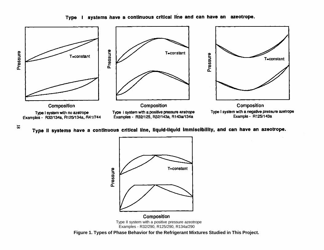
Type II system with a positive pressure azeotropeExamples - R32/290, R125/290, R134a/290
Figure 1. Types of Phase Behavior for the Refrigerant Mixtures Studied in This Project.
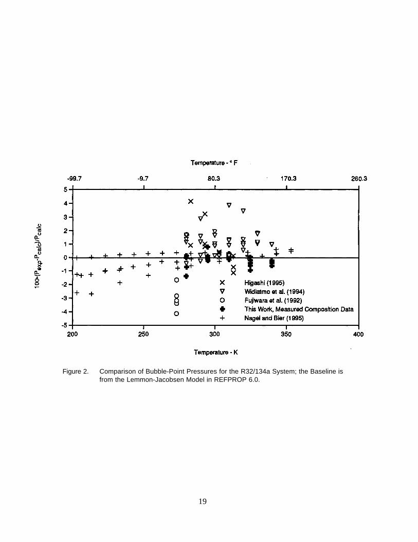
Figure 2. Comparison of Bubble-Point Pressures for the R32/134a System; the Baseline isfrom the Lemmon-Jacobsen Model in REFPROP 6.0.
19
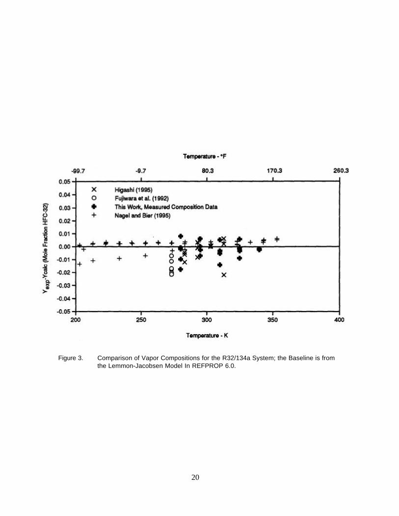
20
Figure 3. Comparison of Vapor Compositions for the R32/134a System; the Baseline is fromthe Lemmon-Jacobsen Model In REFPROP 6.0.
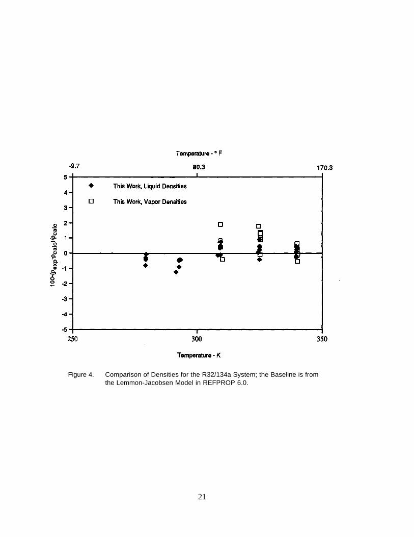
21
Figure 4. Comparison of Densities for the R32/134a System; the Baseline is fromthe Lemmon-Jacobsen Model in REFPROP 6.0.
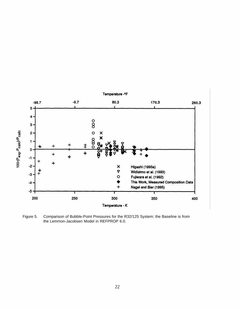
22
Figure 5. Comparison of Bubble-Point Pressures for the R32/125 System; the Baseline is fromthe Lemmon-Jacobsen Model in REFPROP 6.0.
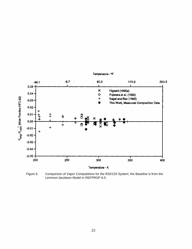
Figure 6. Comparison of Vapor Compositions for the R32/125 System; the Baseline is from theLemmon-Jacobsen Model in REFPROP 6.0.
23
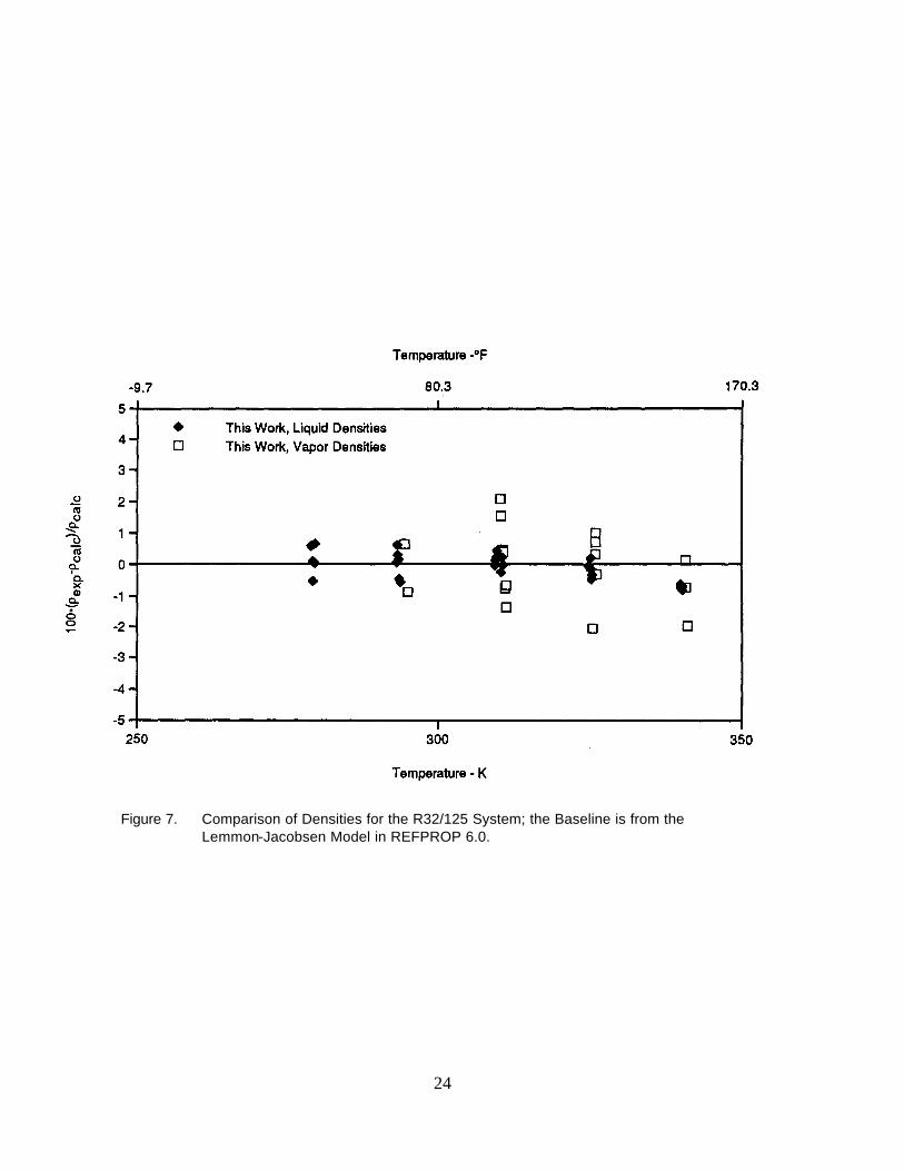
24
Figure 7. Comparison of Densities for the R32/125 System; the Baseline is from theLemmon-Jacobsen Model in REFPROP 6.0.
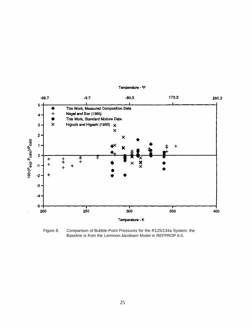
25
Figure 8. Comparison of Bubble-Point Pressures for the R125/134a System; theBaseline is from the Lemmon-Jacobsen Model in REFPROP 6.0.
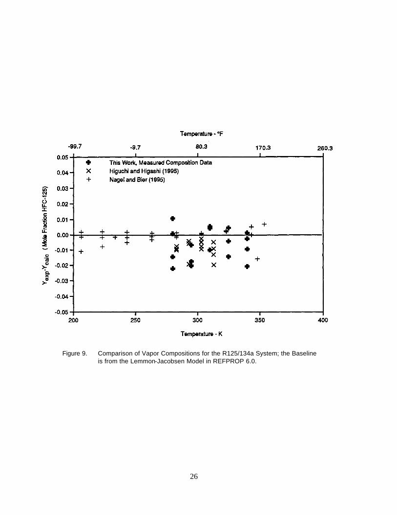
26
Figure 9. Comparison of Vapor Compositions for the R125/134a System; the Baselineis from the Lemmon-Jacobsen Model in REFPROP 6.0.
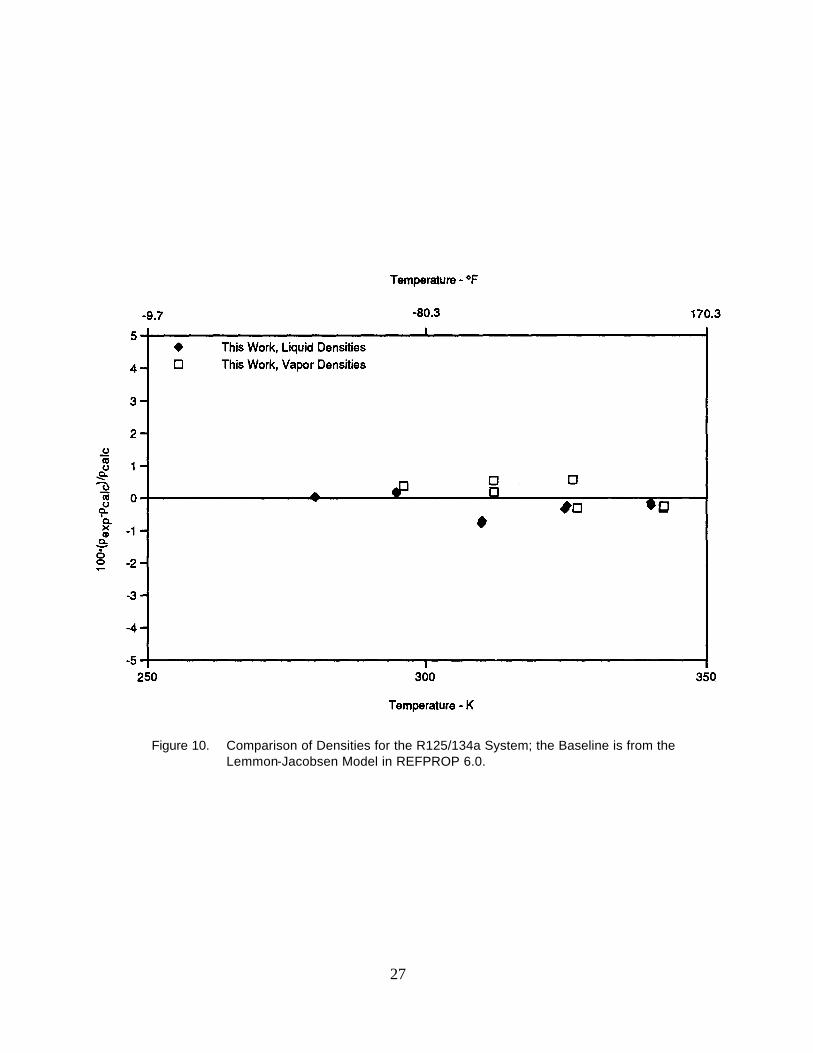
Figure 10. Comparison of Densities for the R125/134a System; the Baseline is from theLemmon-Jacobsen Model in REFPROP 6.0.
27
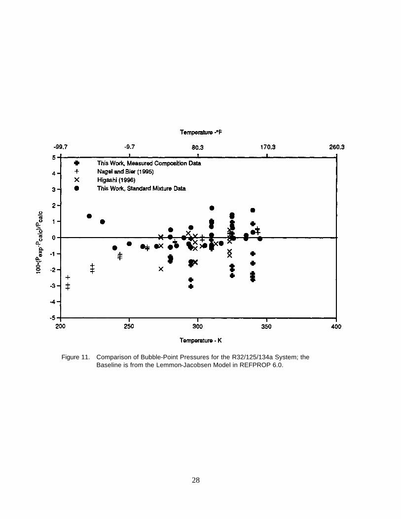
28
Figure 11. Comparison of Bubble-Point Pressures for the R32/125/134a System; theBaseline is from the Lemmon-Jacobsen Model in REFPROP 6.0.

29
Figure 12. Comparison of Vapor Compositions for the R32/125/134a System; theBaseline is from the Lemmon-Jacobsen Model in REFPROP 6.0.

Figure 13. Comparison of Densities for the R32/125/134a System; the Baseline is from theLemmon-Jacobsen Model in REFPROP 6.0.
30

Figure 14. Comparison of Bubble-Point Pressures for the R32/143a System; the Baseline is fromthe Lemmon-Jacobsen Model in REFPROP 6.0.
31
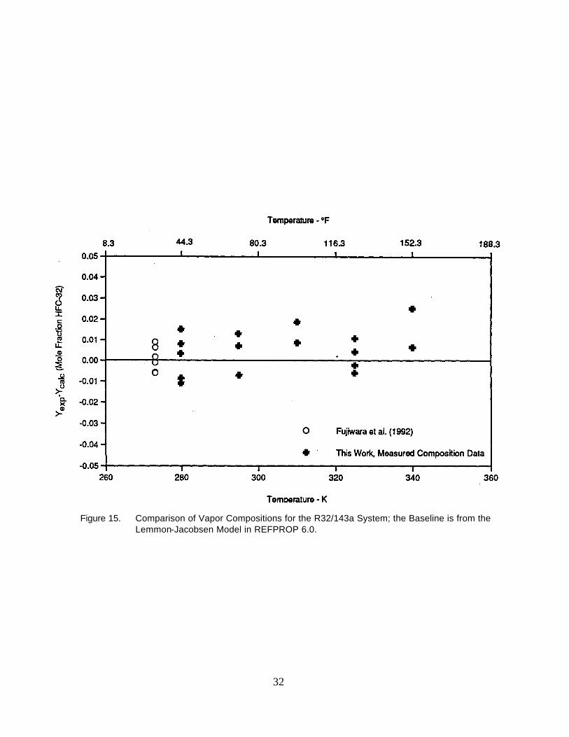
Figure 15. Comparison of Vapor Compositions for the R32/143a System; the Baseline is from theLemmon-Jacobsen Model in REFPROP 6.0.
32
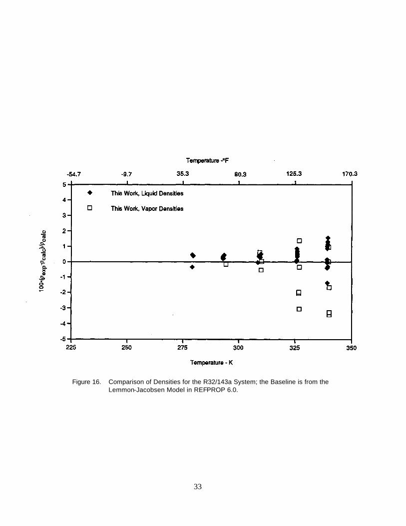
Figure 16. Comparison of Densities for the R32/143a System; the Baseline is from theLemmon-Jacobsen Model in REFPROP 6.0.
33

34
Figure 17. Comparison of Bubble-Point Pressures for the R125/143a System; the Baseline is fromthe Lemmon-Jacobsen Model in REFPROP 6.0.
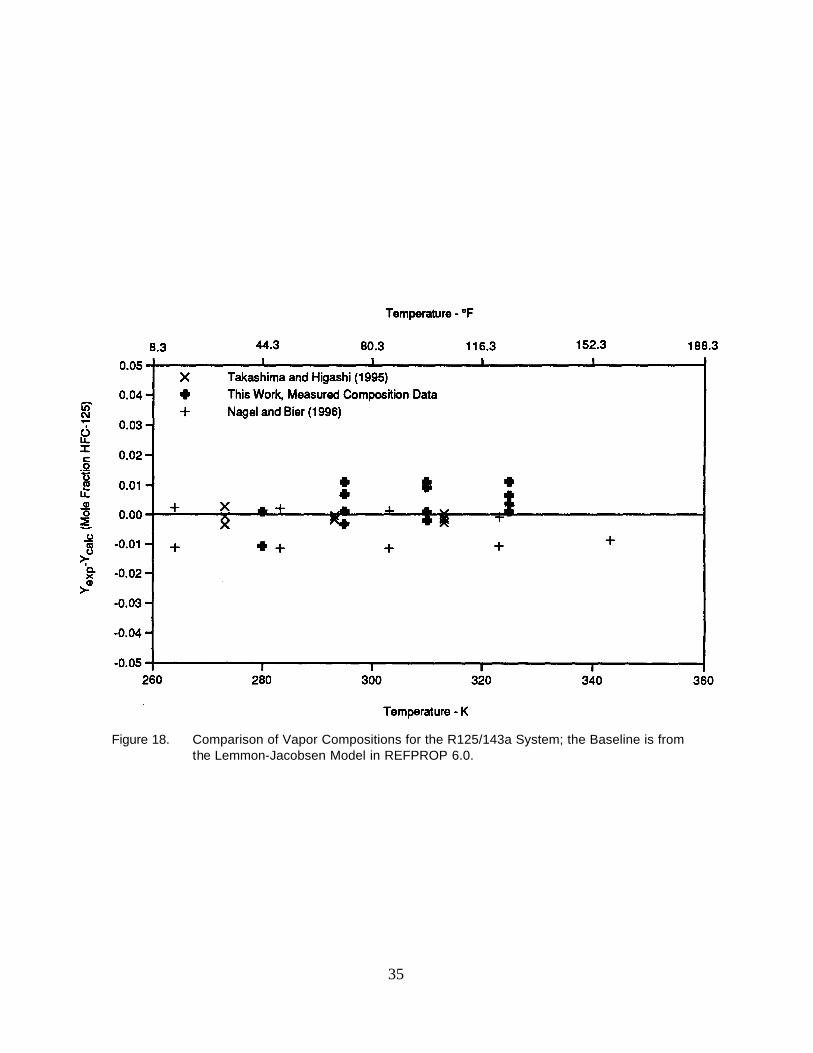
Figure 18. Comparison of Vapor Compositions for the R125/143a System; the Baseline is fromthe Lemmon-Jacobsen Model in REFPROP 6.0.
35
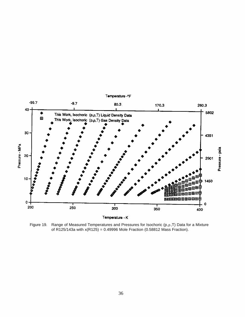
36
Figure 19. Range of Measured Temperatures and Pressures for Isochoric (p,ρ,T) Data for a Mixtureof R125/143a with x(R125) = 0.49996 Mole Fraction (0.58812 Mass Fraction).
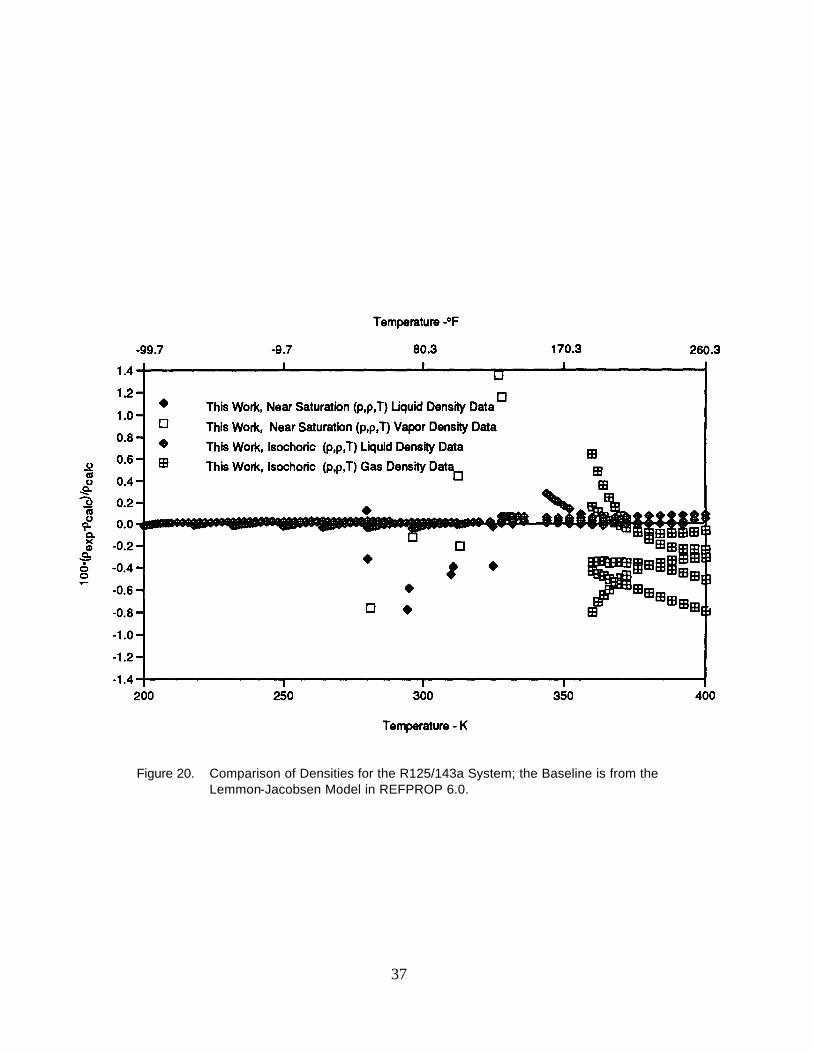
37
Figure 20. Comparison of Densities for the R125/143a System; the Baseline is from theLemmon-Jacobsen Model in REFPROP 6.0.
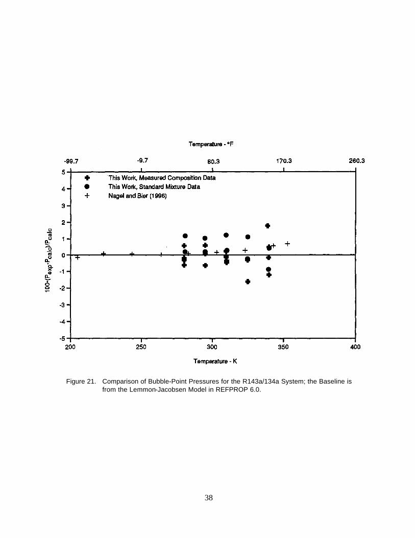
38
Figure 21. Comparison of Bubble-Point Pressures for the R143a/134a System; the Baseline isfrom the Lemmon-Jacobsen Model in REFPROP 6.0.

Figure 22. Comparison of Vapor Compositions for the R143a/134a System; theBaseline is from the Lemmon-Jacobsen Model in REFPROP 6.0.
39

Figure 23. Comparison of Densities for the R143a/134a System; the Baseline is fromthe Lemmon-Jacobsen Model in REFPROP 6.0.
40
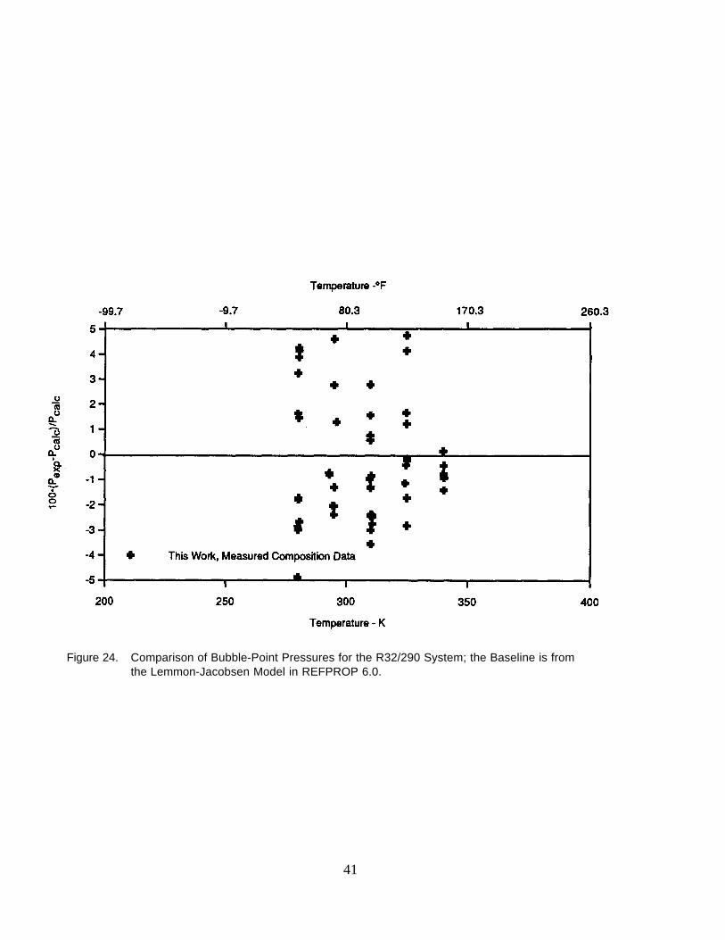
Figure 24. Comparison of Bubble-Point Pressures for the R32/290 System; the Baseline is fromthe Lemmon-Jacobsen Model in REFPROP 6.0.
41
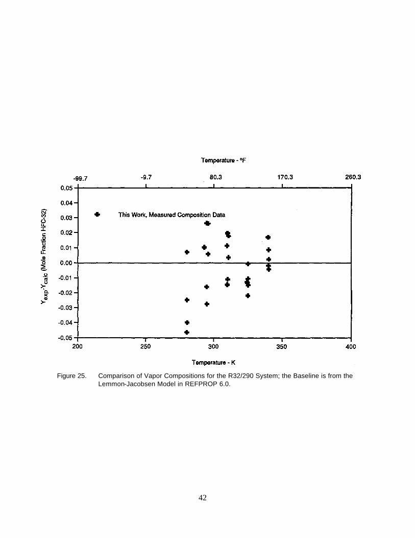
42
Figure 25. Comparison of Vapor Compositions for the R32/290 System; the Baseline is from theLemmon-Jacobsen Model in REFPROP 6.0.
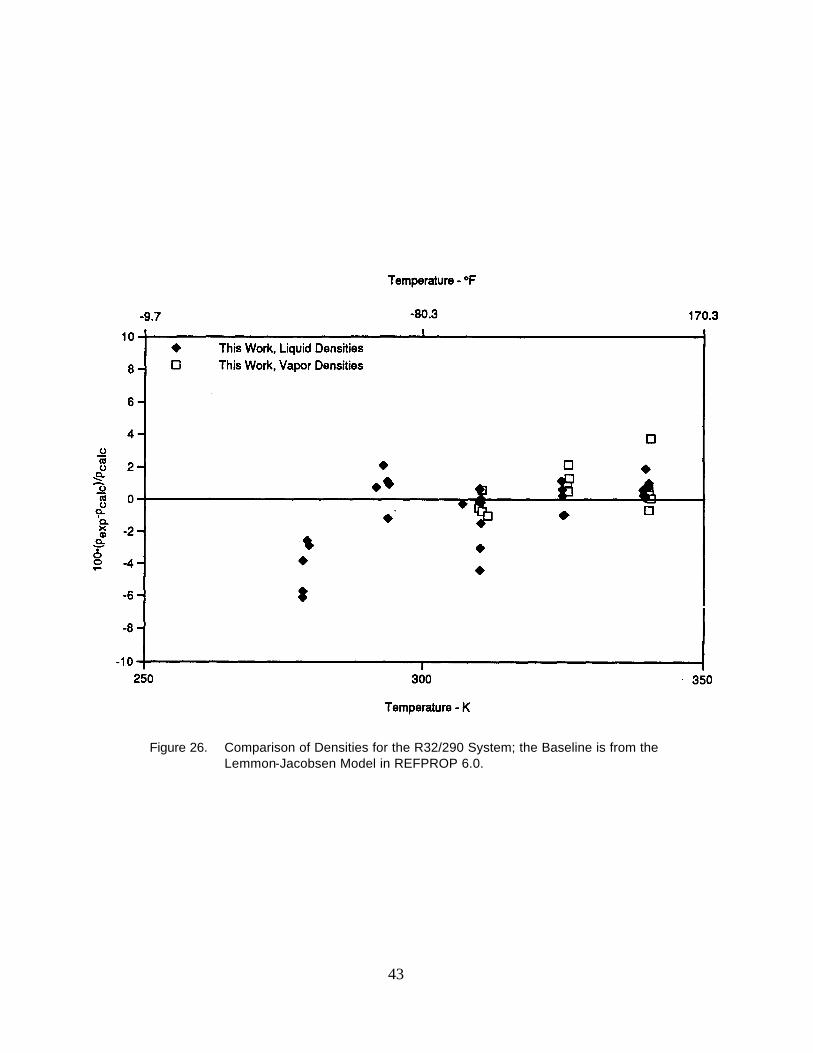
Figure 26. Comparison of Densities for the R32/290 System; the Baseline is from theLemmon-Jacobsen Model in REFPROP 6.0.
43

Figure 27. Comparison of Bubble-Point Pressures for the R125/290 System; the Baseline is fromthe Lemmon-Jacobsen Model in REFPROP 6.0.
44

Figure 28. Comparison of Vapor Compositions for the R125/290 System; the Baseline is from theLemmon-Jacobsen Model in REFPROP 6.0.
45
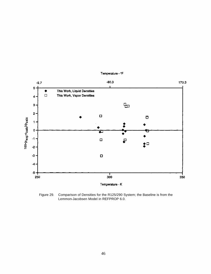
46
Figure 29. Comparison of Densities for the R125/290 System; the Baseline is from theLemmon-Jacobsen Model in REFPROP 6.0.

Figure 30. Comparison of Bubble-Point Pressures for the R134a/290 System; the Baseline isfrom the Lemmon-Jacobsen Model in REFPROP 6.0.
47
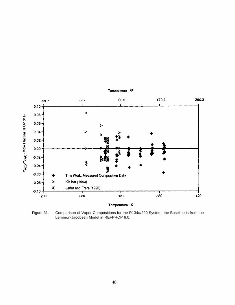
48
Figure 31. Comparison of Vapor Compositions for the R134a/290 System; the Baseline is from theLemmon-Jacobsen Model in REFPROP 6.0.

Figure 32. Comparison of Densities for the R 134a/290 System; the Baseline is from theLemmon-Jacobsen Model in REFPROP 6.0.
49
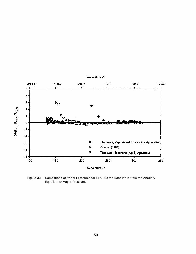
50
Figure 33. Comparison of Vapor Pressures for HFC-41; the Baseline is from the AncillaryEquation for Vapor Pressure.

Figure 34. Range of Measured Temperatures and Pressures for Isochoric (p,ρ,T) Data forHFC-41.
51

Figure 35. Comparison of Densities for HFC-41; the Baseline is from the MBWR Modelin REFPROP 6.0.
52

Figure 36. Deviations of the MBWR Equation of State for HFC-41 from Ancillary Equations forVapor Pressure, Saturated Liquid Density, and Saturated Vapor Density.
53
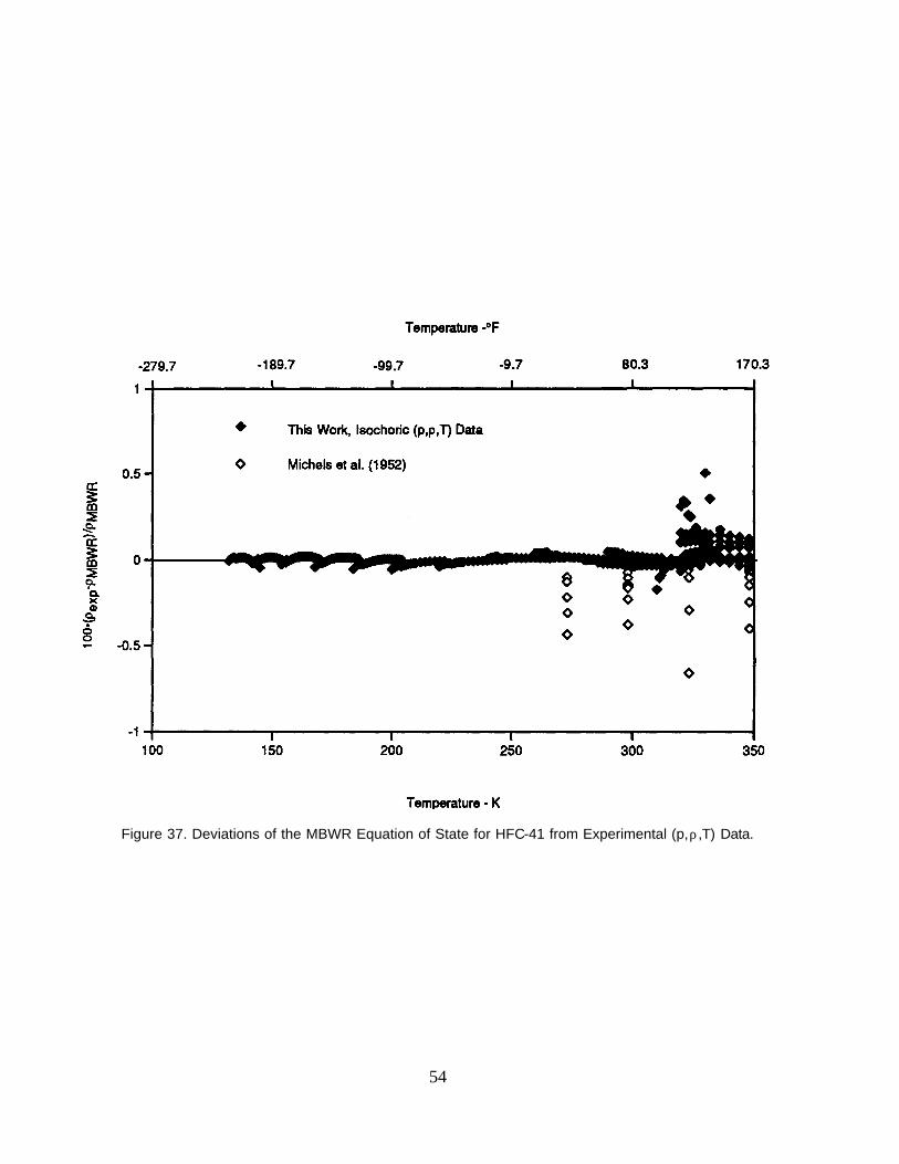
54
Figure 37. Deviations of the MBWR Equation of State for HFC-41 from Experimental (p,ρ,T) Data.
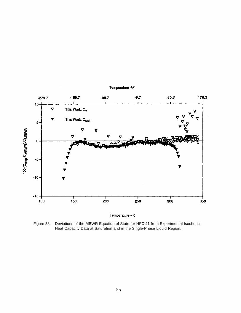
Figure 38. Deviations of the MBWR Equation of State for HFC-41 from Experimental IsochoricHeat Capacity Data at Saturation and in the Single-Phase Liquid Region.
55
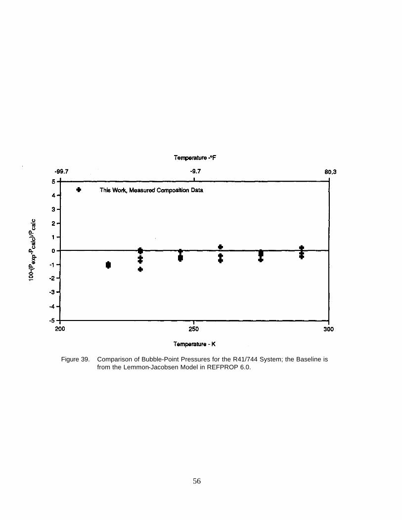
Figure 39. Comparison of Bubble-Point Pressures for the R41/744 System; the Baseline isfrom the Lemmon-Jacobsen Model in REFPROP 6.0.
56
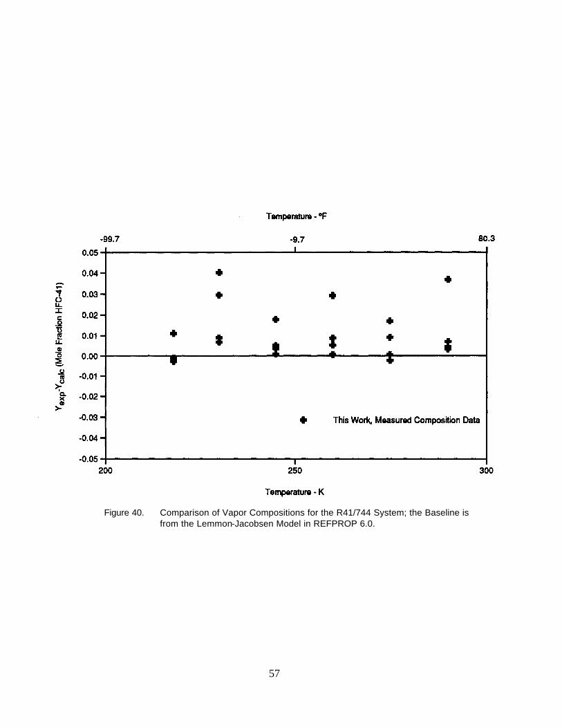
Figure 40. Comparison of Vapor Compositions for the R41/744 System; the Baseline isfrom the Lemmon-Jacobsen Model in REFPROP 6.0.
57

Figure 41. Range of Measured Temperatures and Pressures for Isochoric (p,ρ,T) Data fora Mixture of R41/744 with x(R41) = 0.49982 Mole Fraction (0.43591 MassFraction).
58
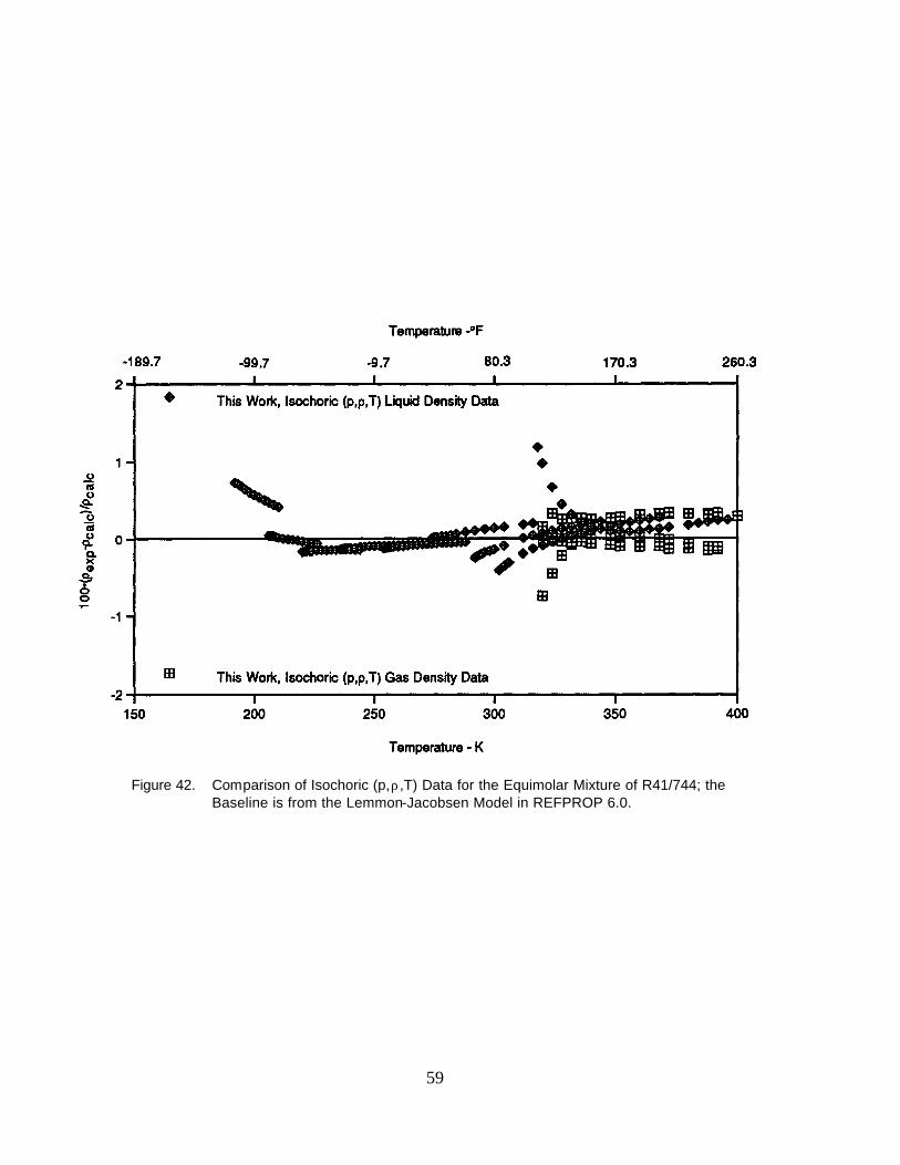
Figure 42. Comparison of Isochoric (p,ρ,T) Data for the Equimolar Mixture of R41/744; theBaseline is from the Lemmon-Jacobsen Model in REFPROP 6.0.
59

A-1
APPENDIX A:
TABLES OF THERMOPHYSICAL PROPERTY DATA
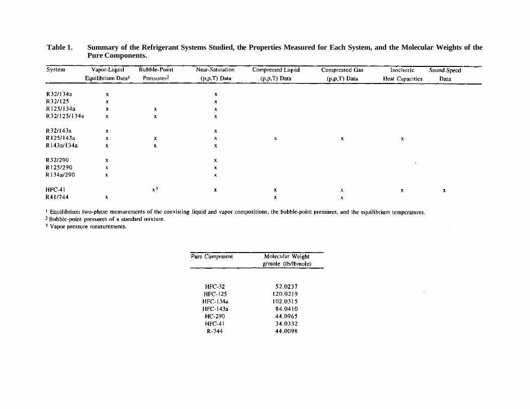
Table 1. Summary of the Refrigerant Systems Studied, the Properties Measured for Each System, and the Molecular Weights of thePure Components.
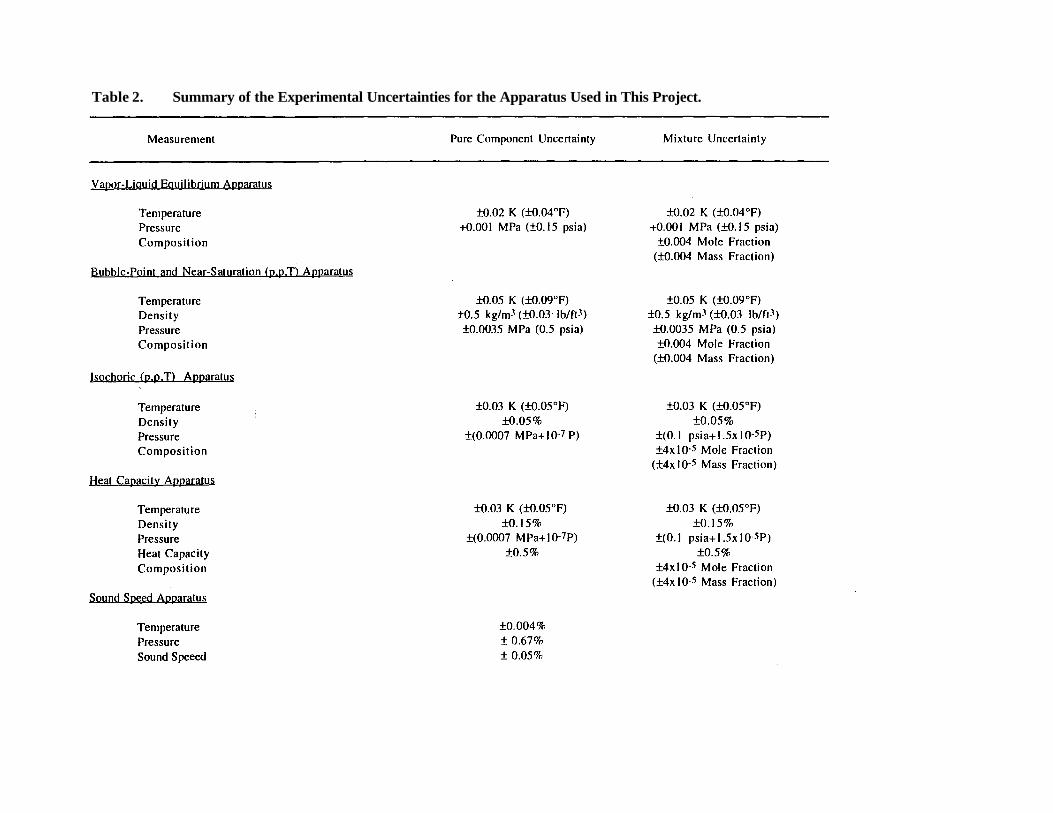
Table 2. Summary of the Experimental Uncertainties for the Apparatus Used in This Project.
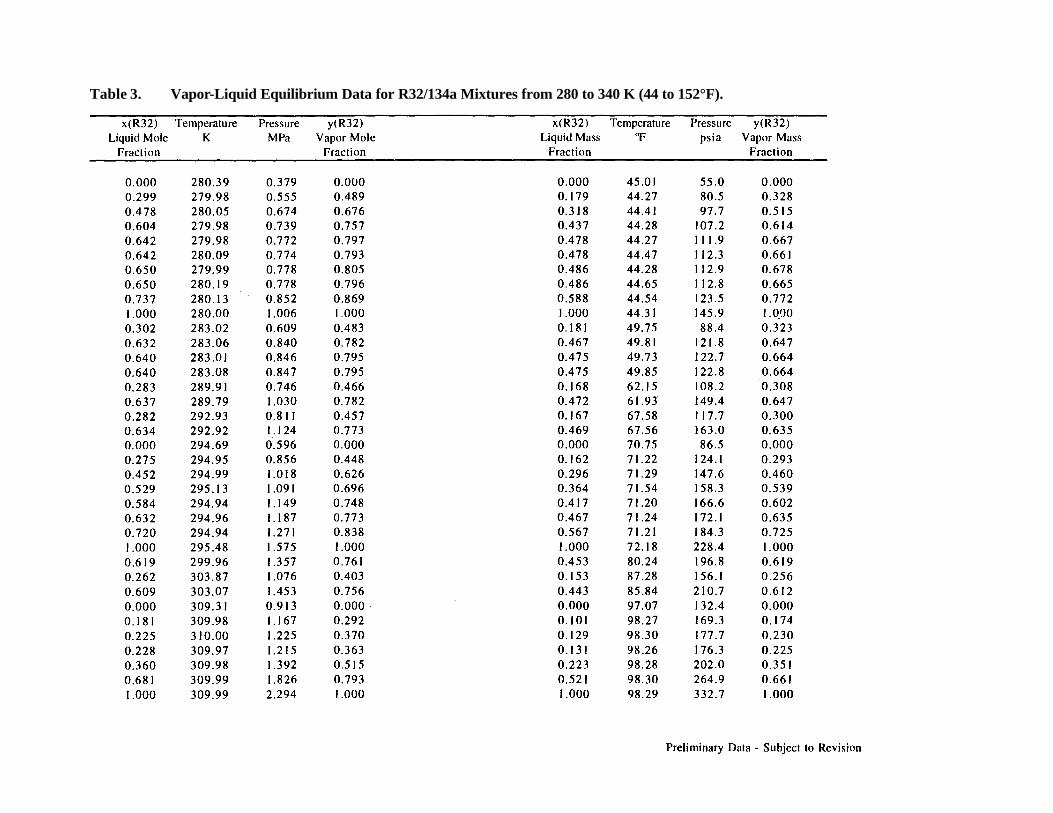
Table 3. Vapor-Liquid Equilibrium Data for R32/134a Mixtures from 280 to 340 K (44 to 152°F).
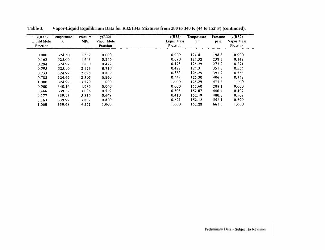
Table 3. Vapor-Liquid Equilibrium Data for R32/134a Mixtures from 280 to 340 K (44 to 152°F) (continued).

Table 4. Near-Saturation (p,ρρ ,T) Data for R32/134aMixtures from 279 to 340 K (43 to 152°F).
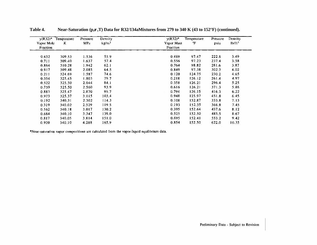
Table 4. Near-Saturation (p,ρρ ,T) Data for R32/134aMixtures from 279 to 340 K (43 to 152°F) (continued).
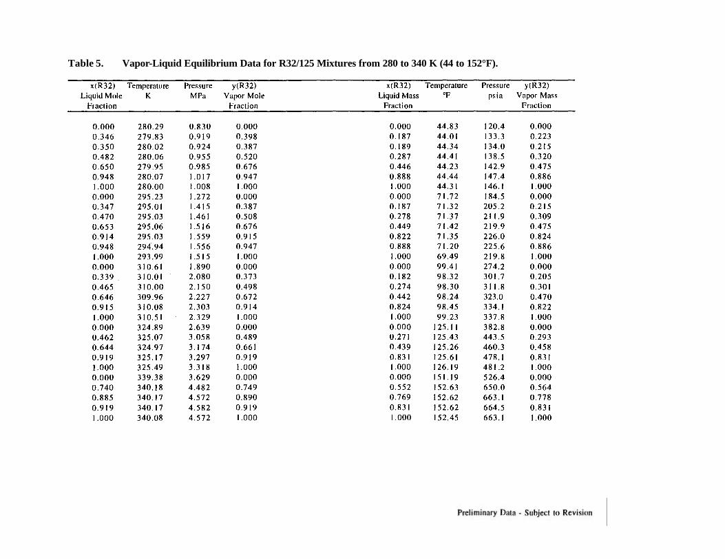
Table 5. Vapor-Liquid Equilibrium Data for R32/125 Mixtures from 280 to 340 K (44 to 152°F).

Table 6. Near-Saturation (p,ρρ ,T) Data for R32/125 Mixtures from 279 to 341 K (43 to 154°F).

Table 6. Near-Saturation (p,ρρ ,T) Data for R32/125 Mixtures from 279 to 341 K (43 to 154°F) (continued).

Table 7. Vapor-Liquid Equilibrium Data for R125/134a Mixtures from 280 to 340 K (44 to 152°F).

Table 8. Bubble -Point Pressures for R125/134a Mixtures from 280 to 340 K (45 to 153°F).

Table 9. Near-Saturation (p,ρρ ,T) Data for R125/134a Mixtures from 280 to 342 K (44 to 157°F).
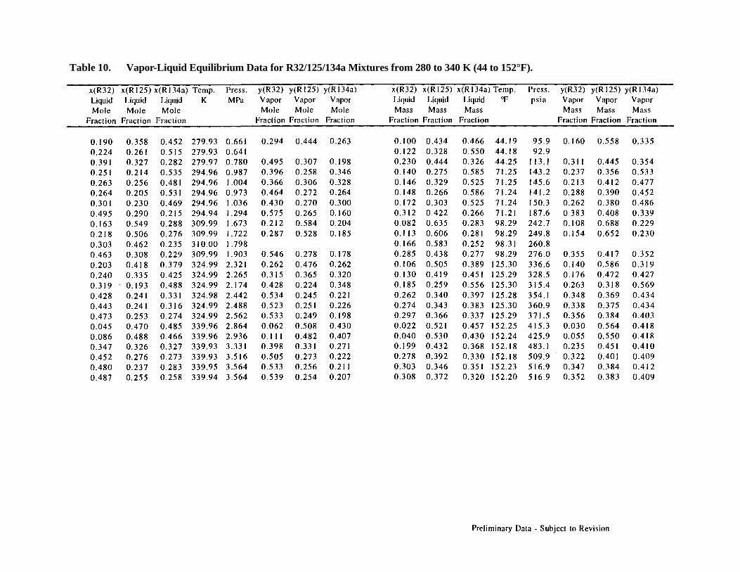
Table 10. Vapor-Liquid Equilibrium Data for R32/125/134a Mixtures from 280 to 340 K (44 to 152°F).

Table 11. Bubble -Point Pressures for R32/125/134a Mixtures from 221 to 345 K (-62 to 162°F).
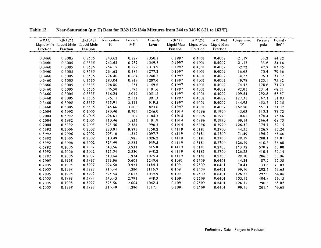
Table 12. Near-Saturation (p,ρρ ,T) Data for R32/125/134a Mixtures from 244 to 346 K (-21 to 163°F).

Table 12. Near-Saturation (p,ρρ ,T) Data for R32/125/134a Mixtures from 244 to 346 K (-21 to 163°F) (continued).
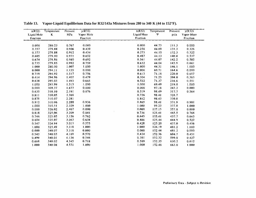
Table 13. Vapor-Liquid Equilibrium Data for R32/143a Mixtures from 280 to 340 K (44 to 152°F).

Table 14. Near-Saturation (p,ρρ ,T) Data for R32/143a Mixtures from 279 to 340 K (43 to 152°F).

Table 14. Near-Saturation (p,ρρ ,T) Data for R32/143a Mixtures from 279 to 340 K (43 to 152°F) (continued).

Table 15. Vapor-Liquid Equilibrium Data for R125/143a Mixtures from 280 to 326 K (44 to 127°F).

Table 16. Bubble -Point Pressures for R125/143a Mixtures from 280 to 325 K (45 to 125°F).
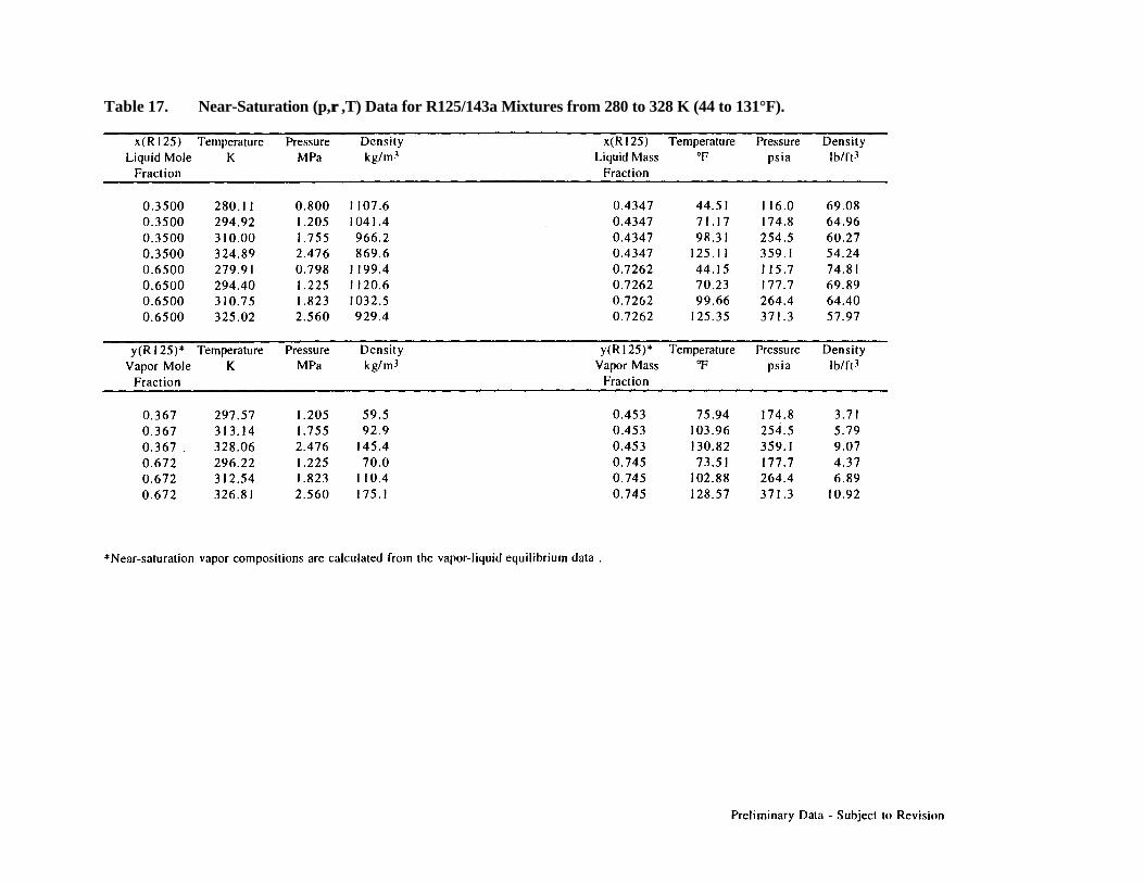
Table 17. Near-Saturation (p,ρρ ,T) Data for R125/143a Mixtures from 280 to 328 K (44 to 131°F).

Table 18. Isochoric (p,ρρ ,T) Data from 200 to 400 K (-100 to 260°F) for a Mixture of R125/143awith x(R125) = 0.49996Mole Fraction (0.58812 Mass Fraction).

Table 18. Isochoric (p,ρρ ,T) Data from 200 to 400 K (-100 to 260°F) for a Mixture of R125/143awith x(R125) = 0.49996 Mole Fraction (0.58812 Mass Fraction) (continued).
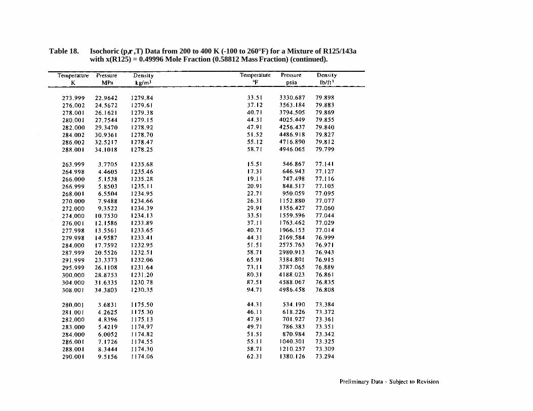
Table 18. Isochoric (p,ρρ ,T) Data from 200 to 400 K (-100 to 260°F) for a Mixture of R125/143awith x(R125) = 0.49996 Mole Fraction (0.58812 Mass Fraction) (continued).

Table 18. Isochoric (p,ρρ ,T) Data from 200 to 400 K (-100 to 260°F) for a Mixture of R125/143awith x(R125) = 0.49996 Mole Fraction (0.58812 Mass Fraction) (continued).

Table 18. Isochoric (p,ρρ ,T) Data from 200 to 400 K (-100 to 260°F) for a Mixture of R125/143awith x(R125) = 0.49996 Mole Fraction (0.58812 Mass Fraction) (continued).

Table 18. Isochoric (p,ρρ ,T) Data from 200 to 400 K (-100 to 260°F) for a Mixture of R125/143awith x(R125) = 0.49996 Mole Fraction (0.58812 Mass Fraction) (continued).
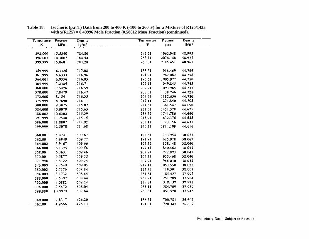
Table 18. Isochoric (p,ρρ ,T) Data from 200 to 400 K (-100 to 260°F) for a Mixture of R125/143awith x(R125) = 0.49996 Mole Fraction (0.58812 Mass Fraction) (continued).

Table 18. Isochoric (p,ρρ ,T) Data from 200 to 400 K (-100 to 260°F) for a Mixture of R125/143awith x(R125) = 0.49996 Mole Fraction (0.58812 Mass Fraction) (continued).
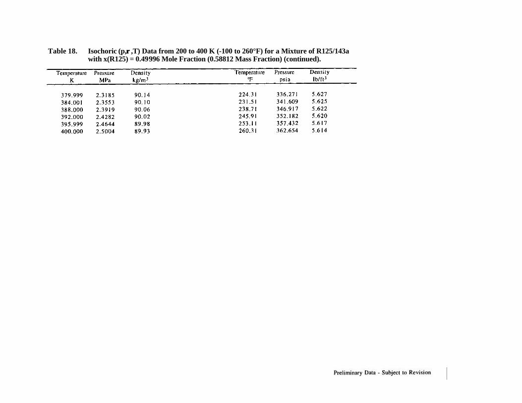
Table 18. Isochoric (p,ρρ ,T) Data from 200 to 400 K (-100 to 260°F) for a Mixture of R125/143awith x(R125) = 0.49996 Mole Fraction (0.58812 Mass Fraction) (continued).
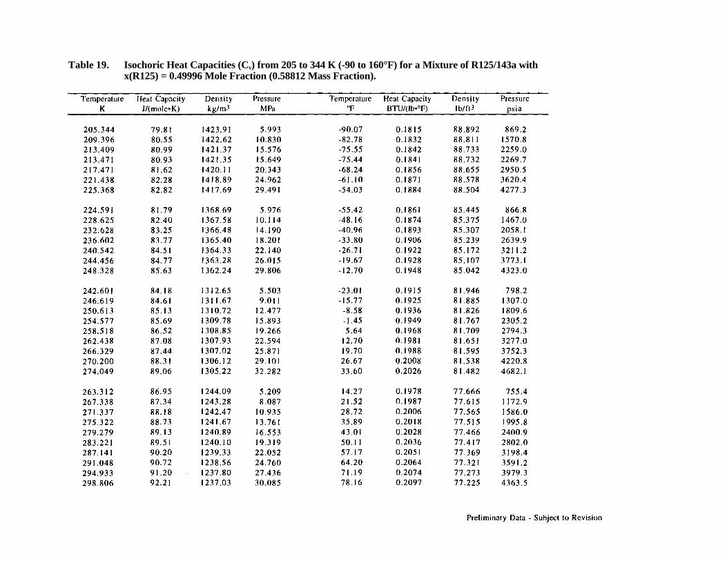
Table 19. Isochoric Heat Capacities (Cv) from 205 to 344 K (-90 to 160°F) for a Mixture of R125/143a withx(R125) = 0.49996 Mole Fraction (0.58812 Mass Fraction).

Table 19. Isochoric Heat Capacities (Cv) from 205 to 344 K (-90 to 160°F) for a Mixture of R125/143a withx(R125) = 0.49996 Mole Fraction (0.58812 Mass Fraction) (continued).
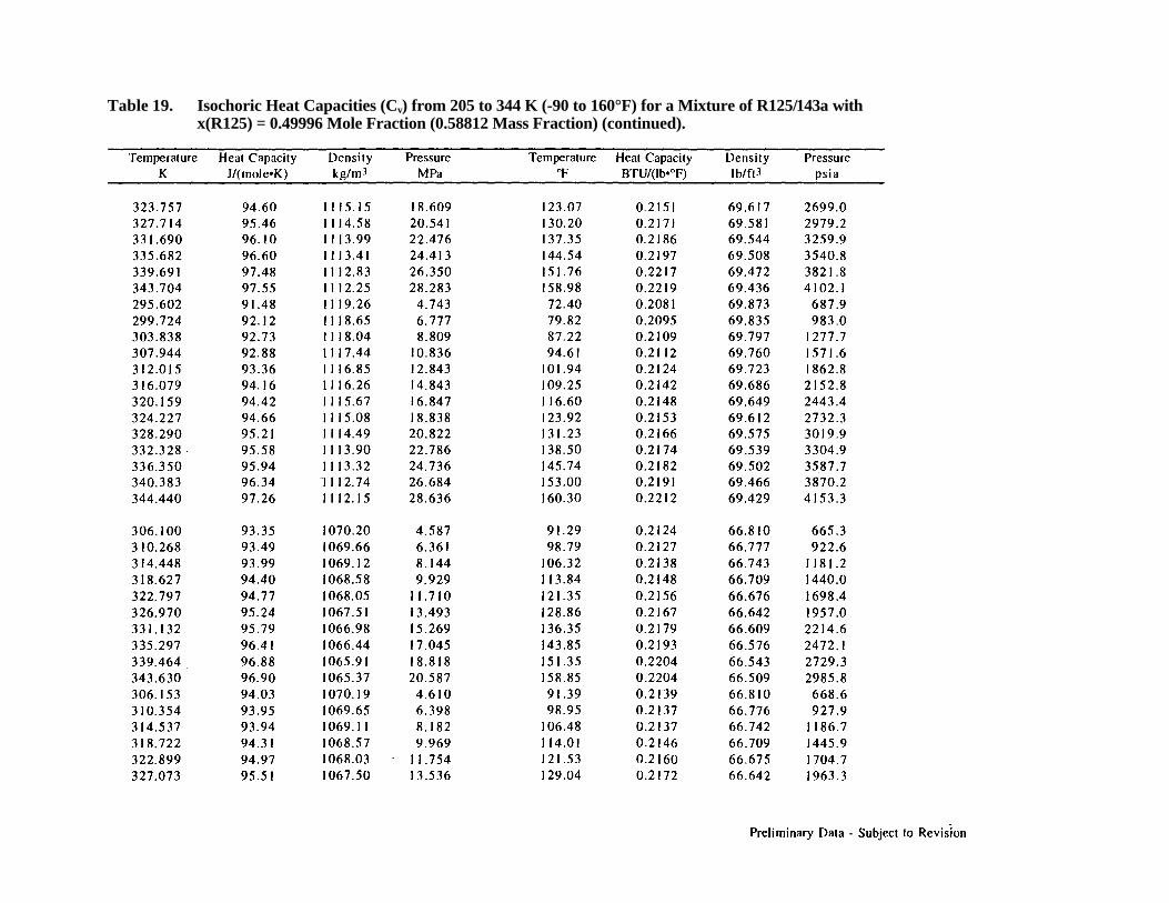
Table 19. Isochoric Heat Capacities (Cv) from 205 to 344 K (-90 to 160°F) for a Mixture of R125/143a withx(R125) = 0.49996 Mole Fraction (0.58812 Mass Fraction) (continued).
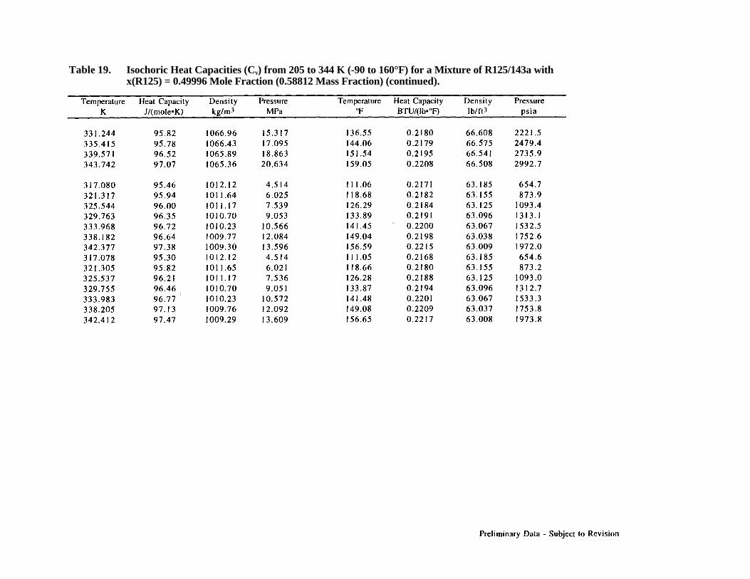
Table 19. Isochoric Heat Capacities (Cv) from 205 to 344 K (-90 to 160°F) for a Mixture of R125/143a withx(R125) = 0.49996 Mole Fraction (0.58812 Mass Fraction) (continued).

Table 20. Vapor-Liquid Equilibrium Data for R143a/134a Mixtures from 280 to 340 K (45 to 152°F).

Table 21. Bubble -Point Pressures for R143a/134a Mixtures from 281 to 340 K (46 to 153°F).
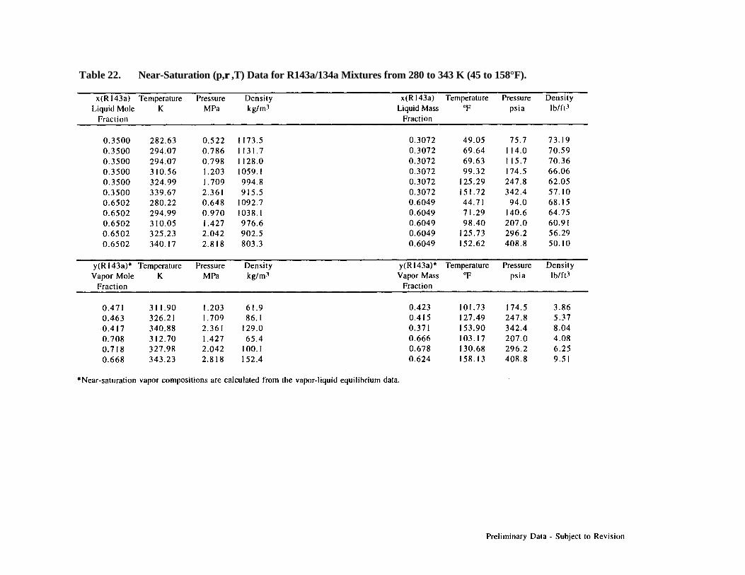
Table 22. Near-Saturation (p,ρρ ,T) Data for R143a/134a Mixtures from 280 to 343 K (45 to 158°F).
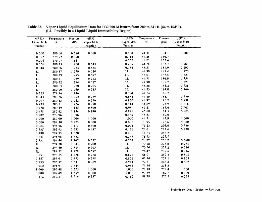
Table 23. Vapor-Liquid Equilibrium Data for R32/290 Mixtures from 280 to 341 K (44 to 154°F).(LL- Possibly in a Liquid-Liquid Immiscibility Region)
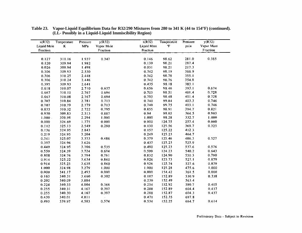
Table 23. Vapor-Liquid Equilibrium Data for R32/290 Mixtures from 280 to 341 K (44 to 154°F) (continued).(LL- Possibly in a Liquid-Liquid Immiscibility Region)
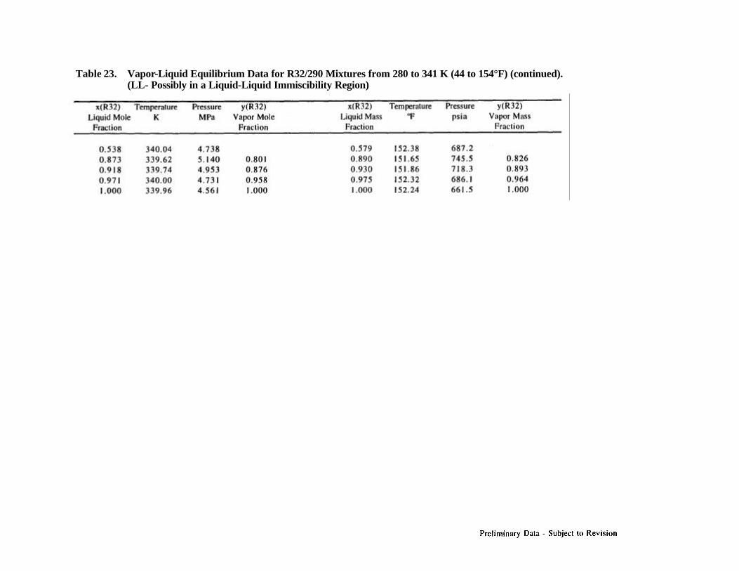
Table 23. Vapor-Liquid Equilibrium Data for R32/290 Mixtures from 280 to 341 K (44 to 154°F) (continued).(LL- Possibly in a Liquid-Liquid Immiscibility Region)

Table 24. Near-Saturation (p,ρρ ,T) Data for R32/290 Mixtures from 278 to 341 K (42 to 153°F).
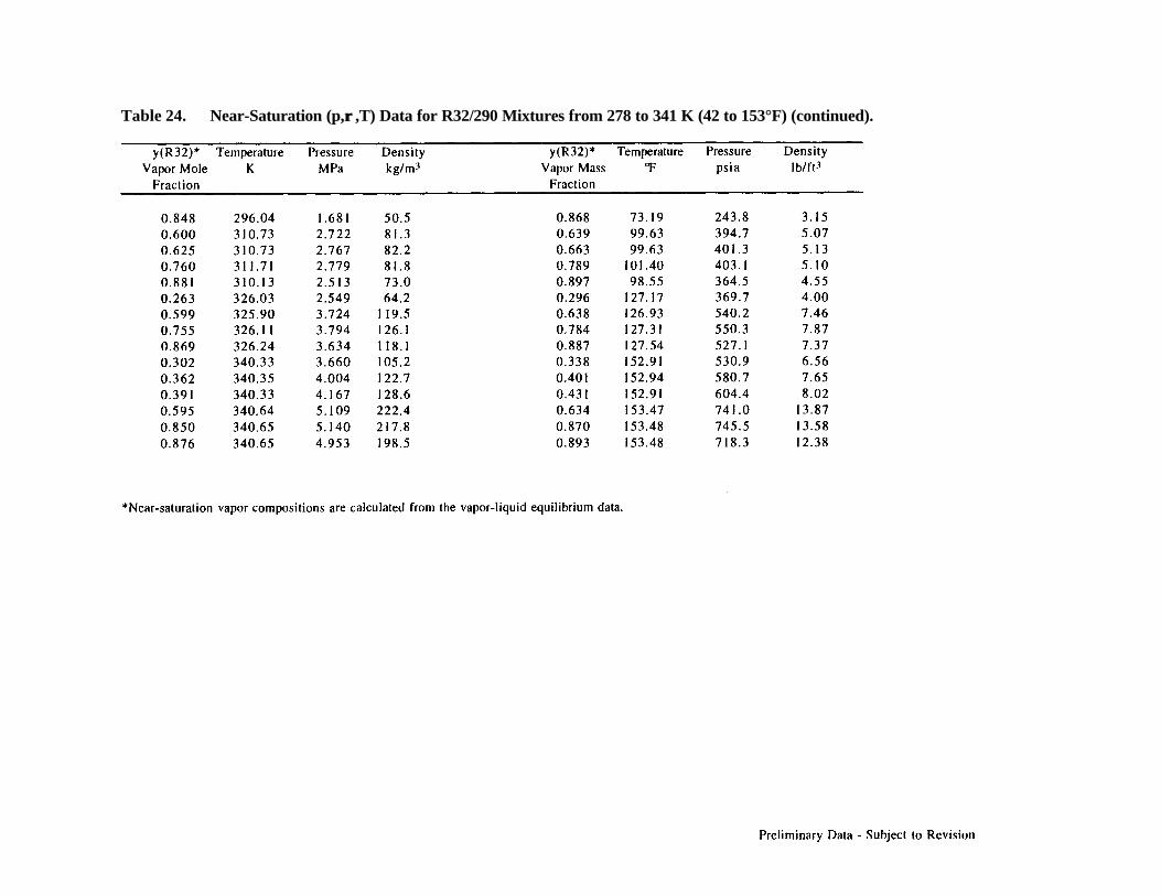
Table 24. Near-Saturation (p,ρρ ,T) Data for R32/290 Mixtures from 278 to 341 K (42 to 153°F) (continued).

Table 25. Vapor-Liquid Equilibrium Data for R125/290 Mixtures from 280 to 364 K (44 to 195°F).
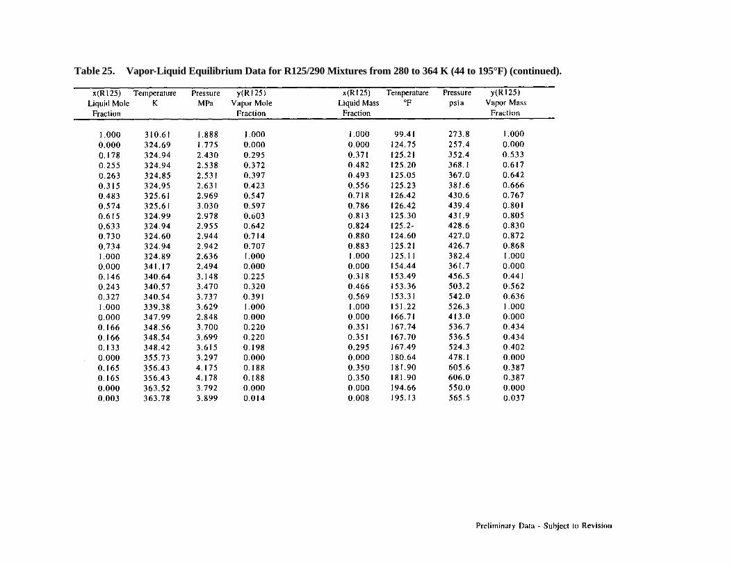
Table 25. Vapor-Liquid Equilibrium Data for R125/290 Mixtures from 280 to 364 K (44 to 195°F) (continued).
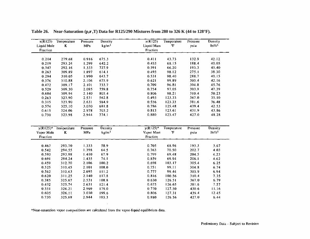
Table 26. Near-Saturation (p,ρρ ,T) Data for R125/290 Mixtures from 280 to 326 K (44 to 128°F).
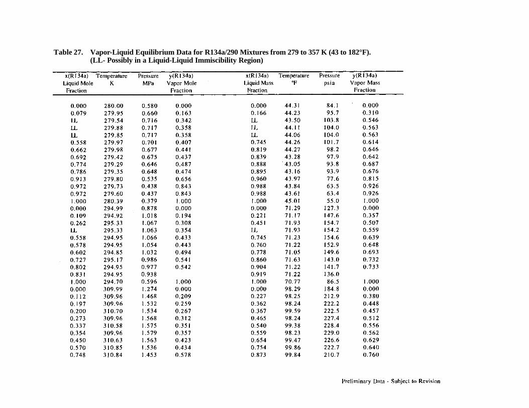
Table 27. Vapor-Liquid Equilibrium Data for R134a/290 Mixtures from 279 to 357 K (43 to 182°F).(LL- Possibly in a Liquid-Liquid Immiscibility Region)

Table 27. Vapor-Liquid Equilibrium Data for R134a/290 Mixtures from 279 to 357 K (43 to 182°F)(continued). (LL- Possibly in a Liquid-Liquid Immiscibility Region)

Table 27. Vapor-Liquid Equilibrium Data for R134a/290 Mixtures from 279 to 357 K (43 to 182°F)(continued). (LL- Possibly in a Liquid-Liquid Immiscibility Region)
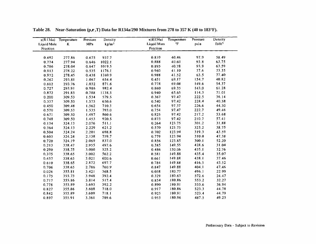
Table 28. Near-Saturation (p,ρρ ,T) Data for R134a/290 Mixtures from 278 to 357 K (40 to 183°F).
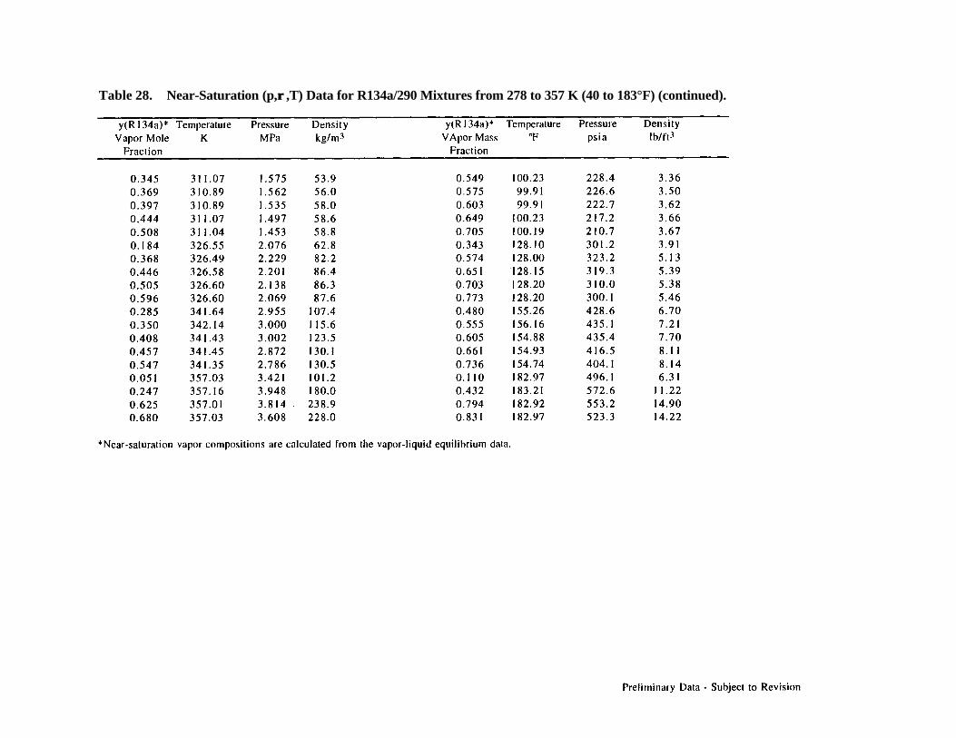
Table 28. Near-Saturation (p,ρρ ,T) Data for R134a/290 Mixtures from 278 to 357 K (40 to 183°F) (continued).
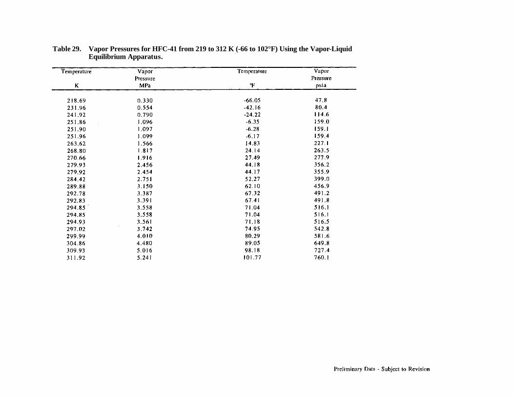
Table 29. Vapor Pressures for HFC-41 from 219 to 312 K (-66 to 102°F) Using the Vapor-LiquidEquilibrium Apparatus.
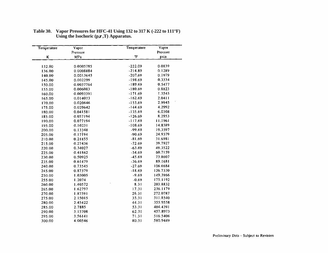
Table 30. Vapor Pressures for HFC-41 Using 132 to 317 K (-222 to 111°F)Using the Isochoric (p,ρρ ,T) Apparatus.
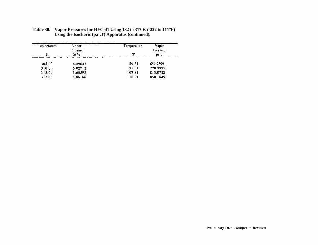
Table 30. Vapor Pressures for HFC-41 Using 132 to 317 K (-222 to 111°F)Using the Isochoric (p,ρρ ,T) Apparatus (continued).
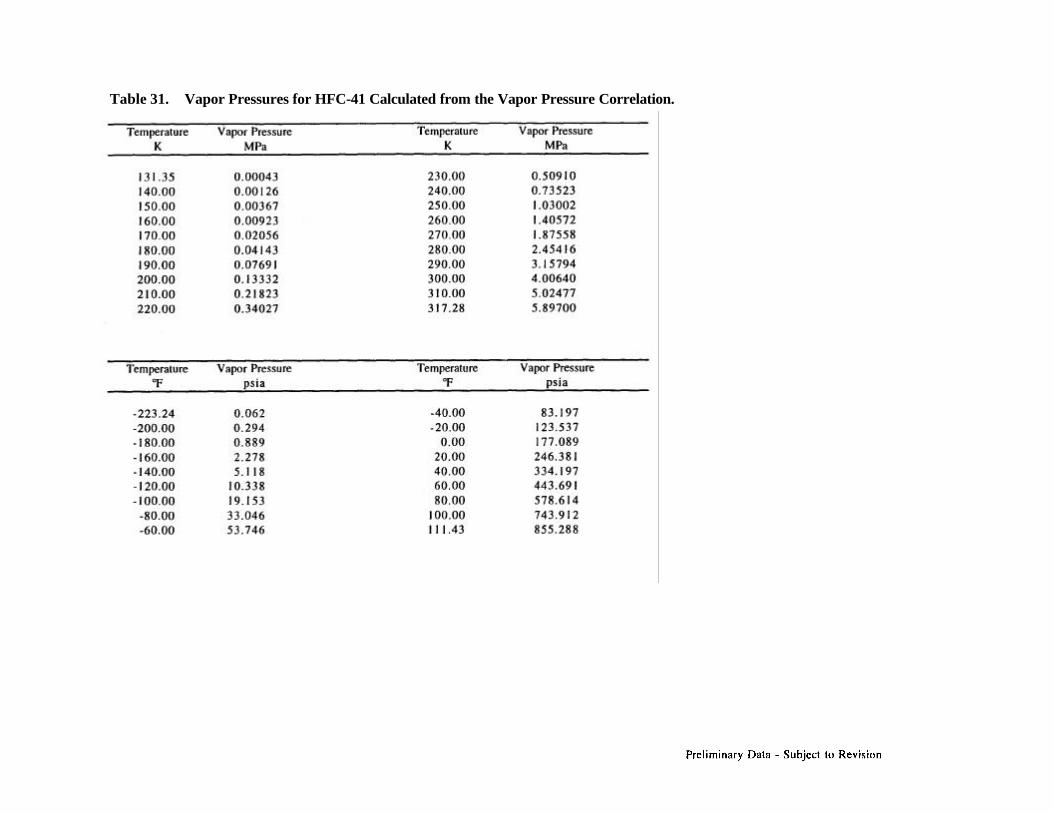
Table 31. Vapor Pressures for HFC-41 Calculated from the Vapor Pressure Correlation.
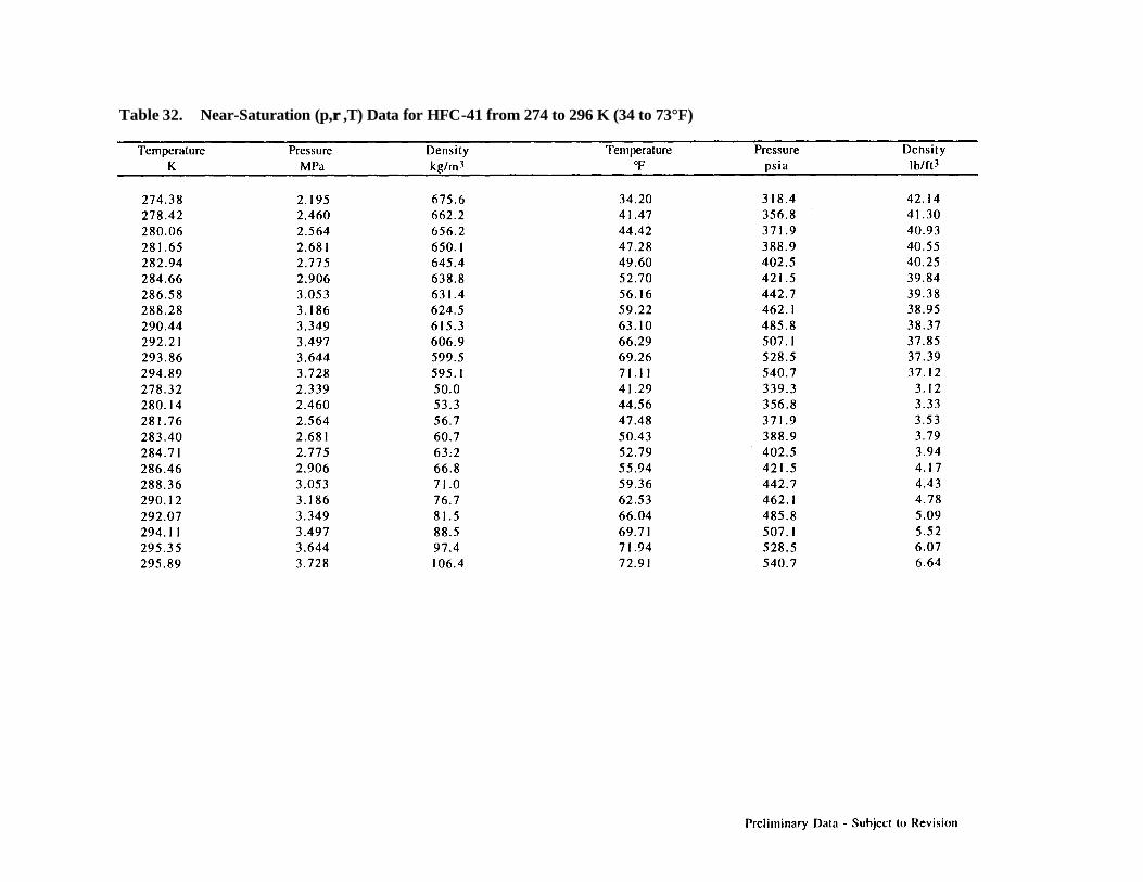
Table 32. Near-Saturation (p,ρρ ,T) Data for HFC-41 from 274 to 296 K (34 to 73°F)
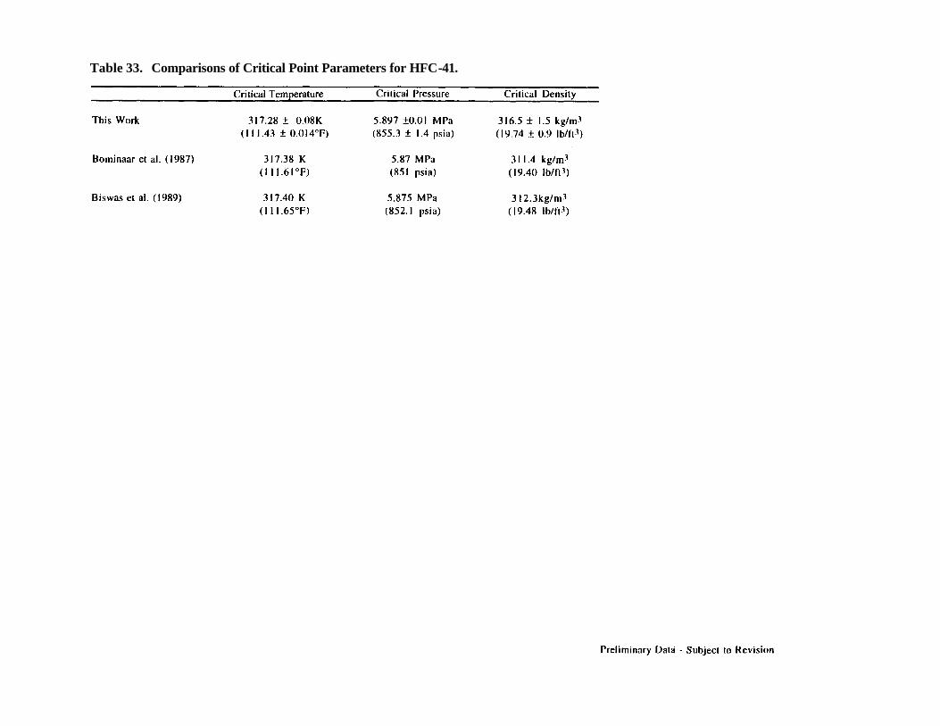
Table 33. Comparisons of Critical Point Parameters for HFC-41.

Table 34. Isochoric (p,ρρ ,T) Data for HFC-41 from 132 to 400 K (-222 to 260°F).

Table 34. Isochoric (p,ρρ ,T) Data for HFC-41 from 132 to 400 K (-222 to 260°F) (continued).

Table 34. Isochoric (p,ρρ ,T) Data for HFC-41 from 132 to 400 K (-222 to 260°F) (continued).
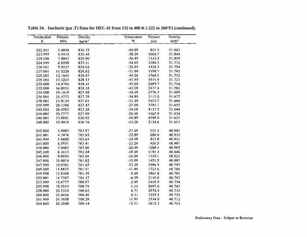
Table 34. Isochoric (p,ρρ ,T) Data for HFC-41 from 132 to 400 K (-222 to 260°F) (continued).

Table 34. Isochoric (p,ρρ ,T) Data for HFC-41 from 132 to 400 K (-222 to 260°F) (continued).

Table 34. Isochoric (p,ρρ ,T) Data for HFC-41 from 132 to 400 K (-222 to 260°F) (continued).
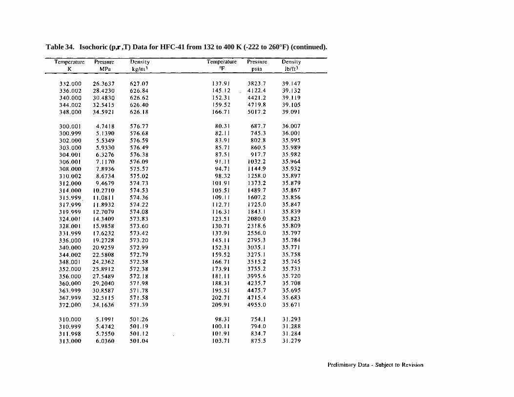
Table 34. Isochoric (p,ρρ ,T) Data for HFC-41 from 132 to 400 K (-222 to 260°F) (continued).

Table 34. Isochoric (p,ρρ ,T) Data for HFC-41 from 132 to 400 K (-222 to 260°F) (continued).

Table 34. Isochoric (p,ρρ ,T) Data for HFC-41 from 132 to 400 K (-222 to 260°F) (continued).

Table 34. Isochoric (p,ρρ ,T) Data for HFC-41 from 132 to 400 K (-222 to 260°F) (continued).

Table 34. Isochoric (p,ρρ ,T) Data for HFC-41 from 132 to 400 K (-222 to 260°F) (continued).

Table 34. Isochoric (p,ρρ ,T) Data for HFC-41 from 132 to 400 K (-222 to 260°F) (continued).
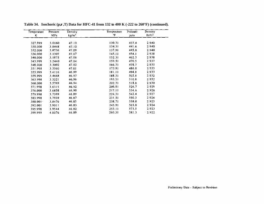
Table 34. Isochoric (p,ρρ ,T) Data for HFC-41 from 132 to 400 K (-222 to 260°F) (continued).
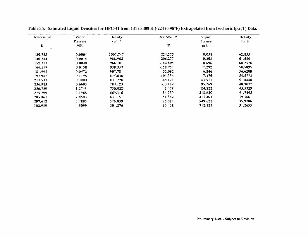
Table 35. Saturated Liquid Densities for HFC-41 from 131 to 309 K (-224 to 96°F) Extrapolated from Isochoric (p,ρρ ,T) Data.

Table 36. Isochoric Heat Capacities (Cv) for HFC-41 from 148 to 343 K (-193 to 157°F).

Table 36. Isochoric Heat Capacities (Cv) for HFC-41 from 148 to 343 K (-193 to 157°F) (continued).
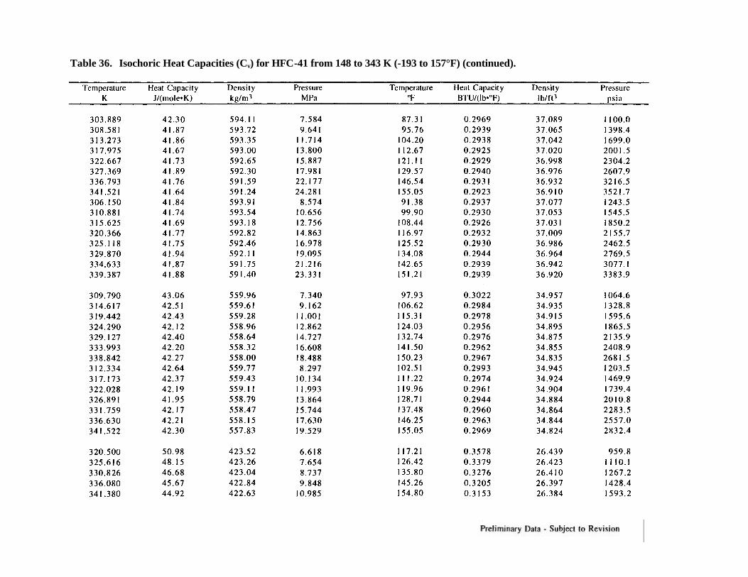
Table 36. Isochoric Heat Capacities (Cv) for HFC-41 from 148 to 343 K (-193 to 157°F) (continued).

Table 36. Isochoric Heat Capacitie s (Cv) for HFC-41 from 148 to 343 K (-193 to 157°F) (continued).

Table 37. Two-Phase Heat Capacities for HFC-41 from 136 to 314 K (-215 to 106°F).

Table 37. Two-Phase Heat Capacities for HFC-41 from 136 to 314 K (-215 to 106°F) (continued).

Table 37. Two-Phase Heat Capacities for HFC-41 from 136 to 314 K (-215 to 106°F) (continued).
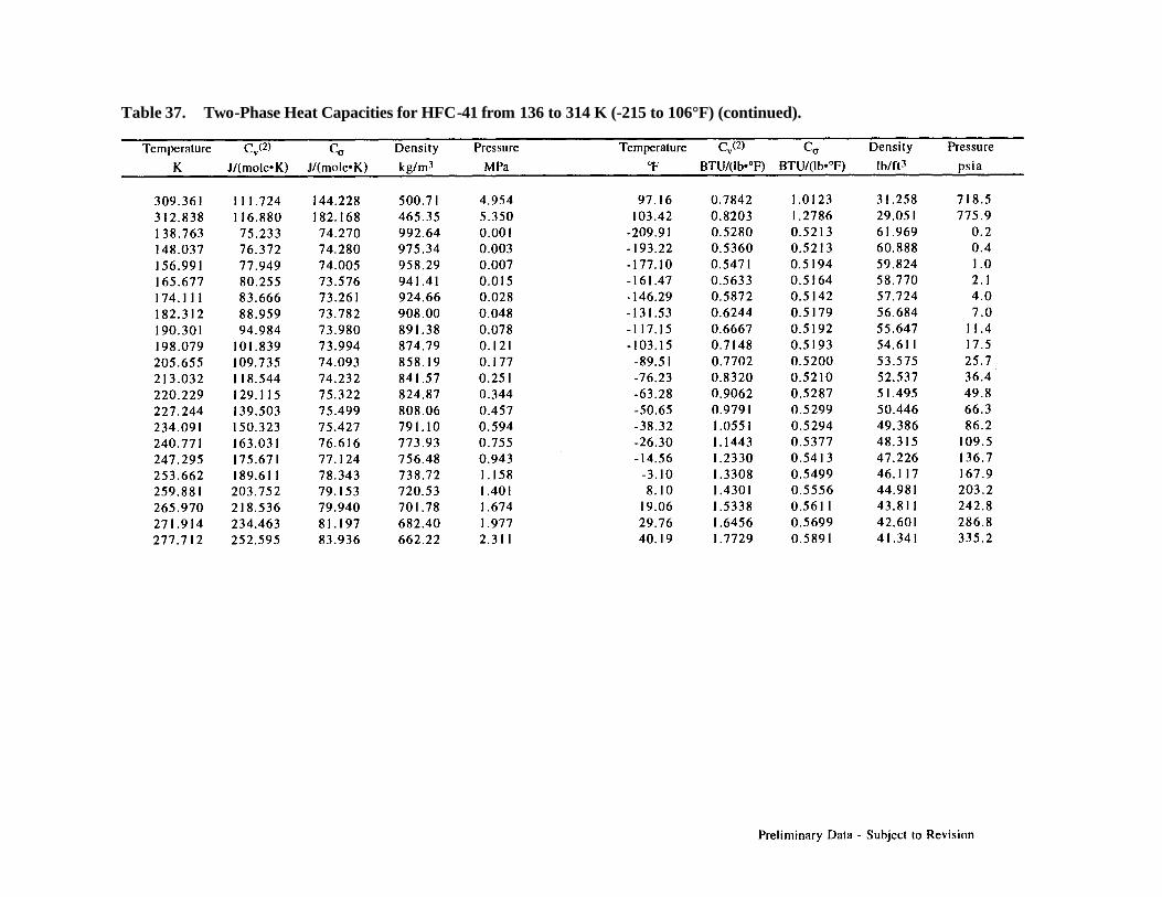
Table 37. Two-Phase Heat Capacities for HFC-41 from 136 to 314 K (-215 to 106°F) (continued).

Table 38. Vapor-Phase Sound Speed Data for HFC-41 from 249.5 to350 K (-11 to 170°F).
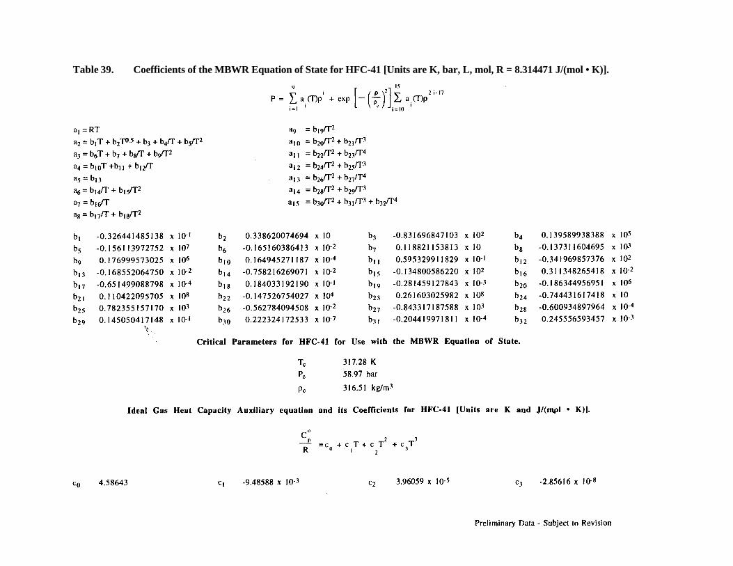
Table 39. Coefficients of the MBWR Equation of State for HFC-41 [Units are K, bar, L, mol, R = 8.314471 J/(mol • K)].

Table 40. Vapor-Liquid Equilibrium Data for R41/744 Mixtures from 218 to 290 K (-68 to 62°F).

Table 40. Vapor-Liquid Equilibrium Data for R41/744 Mixtures from 218 to 290 K (-68 to 62°F) (continued).
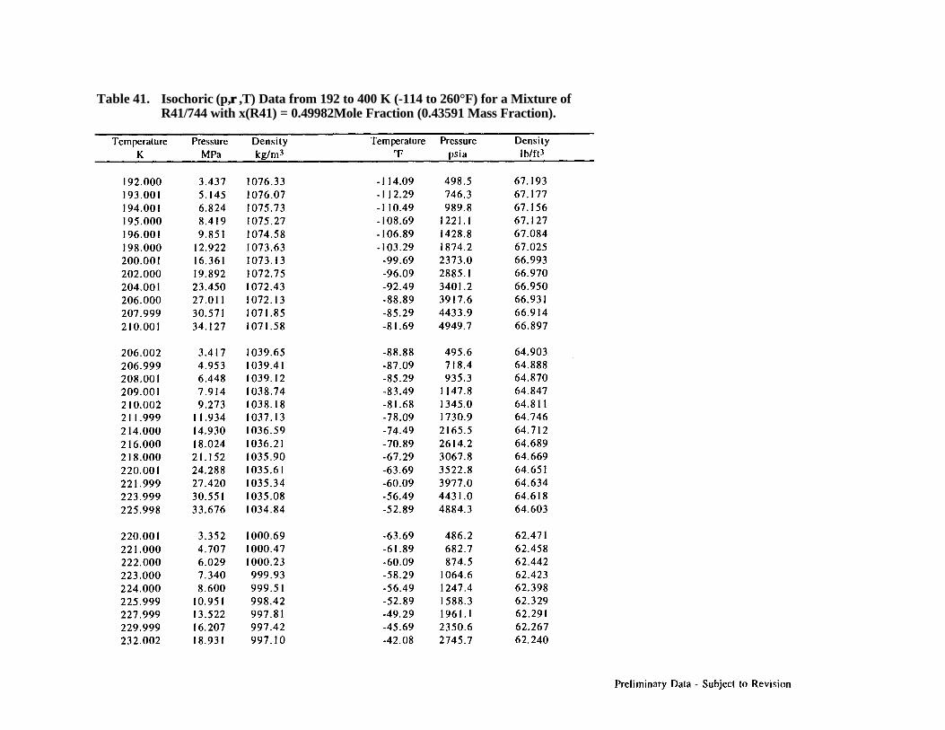
Table 41. Isochoric (p,ρρ ,T) Data from 192 to 400 K (-114 to 260°F) for a Mixture ofR41/744 with x(R41) = 0.49982Mole Fraction (0.43591 Mass Fraction).
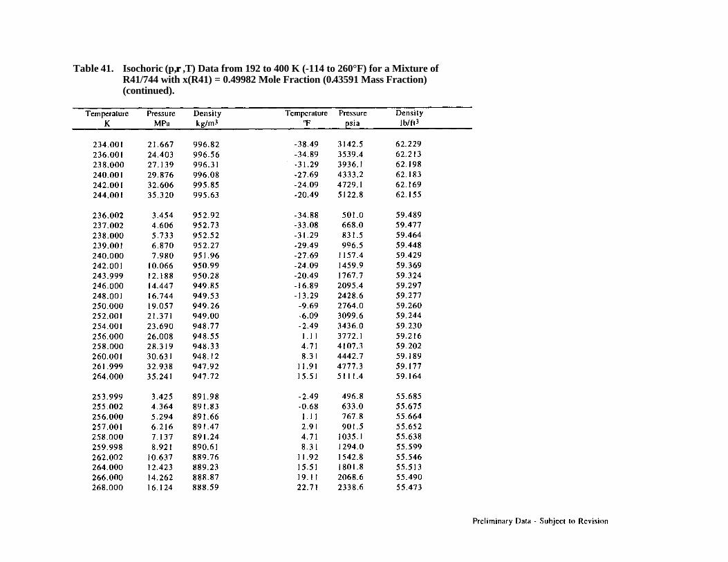
Table 41. Isochoric (p,ρρ ,T) Data from 192 to 400 K (-114 to 260°F) for a Mixture ofR41/744 with x(R41) = 0.49982 Mole Fraction (0.43591 Mass Fraction)(continued).

Table 41. Isochoric (p,ρρ ,T) Data from 192 to 400 K (-114 to 260°F) for a Mixture ofR41/744 with x(R41) = 0.49982 Mole Fraction (0.43591 Mass Fraction)(continued).

Table 41. Isochoric (p,ρρ ,T) Data from 192 to 400 K (-114 to 260°F) for a Mixture ofR41/744 with x(R41) = 0.49982 Mole Fraction (0.43591 Mass Fraction)(continued).

Table 41. Isochoric (p,ρρ ,T) Data from 192 to 400 K (-114 to 260°F) for a Mixture ofR41/744 with x(R41) = 0.49982 Mole Fraction (0.43591 Mass Fraction)(continued).
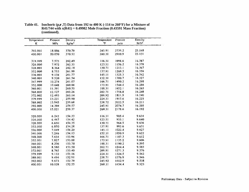
Table 41. Isochoric (p,ρρ ,T) Data from 192 to 400 K (-114 to 260°F) for a Mixture ofR41/744 with x(R41) = 0.49982 Mole Fraction (0.43591 Mass Fraction)(continued).

Table 41. Isochoric (p,ρρ ,T) Data from 192 to 400 K (-114 to 260°F) for a Mixture ofR41/744 with x(R41) = 0.49982 Mole Fraction (0.43591 Mass Fraction)(continued).

Table 42. Summary of the Interaction Parameters for the Lemmon-JacobsenModel for the Systems Studied in This Project.

APPENDIX B:
EXPERIMENTAL APPARATUS
B-1
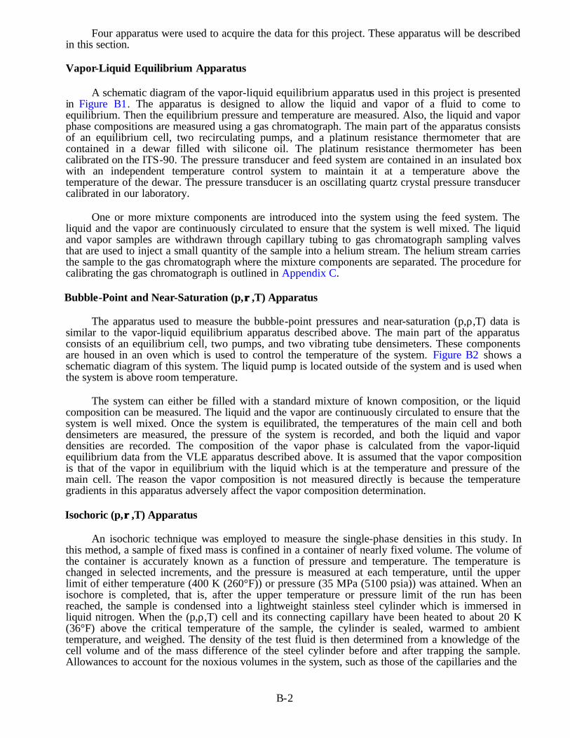
Four apparatus were used to acquire the data for this project. These apparatus will be describedin this section.
Vapor-Liquid Equilibrium Apparatus
A schematic diagram of the vapor-liquid equilibrium apparatus used in this project is presentedin Figure B1. The apparatus is designed to allow the liquid and vapor of a fluid to come toequilibrium. Then the equilibrium pressure and temperature are measured. Also, the liquid and vaporphase compositions are measured using a gas chromatograph. The main part of the apparatus consistsof an equilibrium cell, two recirculating pumps, and a platinum resistance thermometer that arecontained in a dewar filled with silicone oil. The platinum resistance thermometer has beencalibrated on the ITS-90. The pressure transducer and feed system are contained in an insulated boxwith an independent temperature control system to maintain it at a temperature above thetemperature of the dewar. The pressure transducer is an oscillating quartz crystal pressure transducercalibrated in our laboratory.
One or more mixture components are introduced into the system using the feed system. Theliquid and the vapor are continuously circulated to ensure that the system is well mixed. The liquidand vapor samples are withdrawn through capillary tubing to gas chromatograph sampling valvesthat are used to inject a small quantity of the sample into a helium stream. The helium stream carriesthe sample to the gas chromatograph where the mixture components are separated. The procedure forcalibrating the gas chromatograph is outlined in Appendix C.
Bubble-Point and Near-Saturation (p,ρρ ,T) Apparatus
The apparatus used to measure the bubble-point pressures and near-saturation (p,ρ,T) data issimilar to the vapor-liquid equilibrium apparatus described above. The main part of the apparatusconsists of an equilibrium cell, two pumps, and two vibrating tube densimeters. These componentsare housed in an oven which is used to control the temperature of the system. Figure B2 shows aschematic diagram of this system. The liquid pump is located outside of the system and is used whenthe system is above room temperature.
The system can either be filled with a standard mixture of known composition, or the liquidcomposition can be measured. The liquid and the vapor are continuously circulated to ensure that thesystem is well mixed. Once the system is equilibrated, the temperatures of the main cell and bothdensimeters are measured, the pressure of the system is recorded, and both the liquid and vapordensities are recorded. The composition of the vapor phase is calculated from the vapor-liquidequilibrium data from the VLE apparatus described above. It is assumed that the vapor compositionis that of the vapor in equilibrium with the liquid which is at the temperature and pressure of themain cell. The reason the vapor composition is not measured directly is because the temperaturegradients in this apparatus adversely affect the vapor composition determination.
Isochoric (p,ρρ ,T) Apparatus
An isochoric technique was employed to measure the single-phase densities in this study. Inthis method, a sample of fixed mass is confined in a container of nearly fixed volume. The volume ofthe container is accurately known as a function of pressure and temperature. The temperature ischanged in selected increments, and the pressure is measured at each temperature, until the upperlimit of either temperature (400 K (260°F)) or pressure (35 MPa (5100 psia)) was attained. When anisochore is completed, that is, after the upper temperature or pressure limit of the run has beenreached, the sample is condensed into a lightweight stainless steel cylinder which is immersed inliquid nitrogen. When the (p,ρ,T) cell and its connecting capillary have been heated to about 20 K(36°F) above the critical temperature of the sample, the cylinder is sealed, warmed to ambienttemperature, and weighed. The density of the test fluid is then determined from a knowledge of thecell volume and of the mass difference of the steel cylinder before and after trapping the sample.Allowances to account for the noxious volumes in the system, such as those of the capillaries and the
B-2
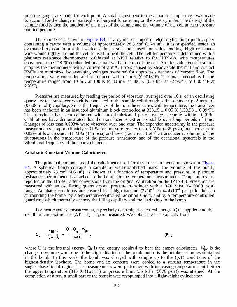
pressure gauge, are made for each point. A small adjustment to the apparent sample mass was madeto account for the change in atmospheric buoyant force acting on the steel cylinder. The density of thesample fluid is then the quotient of the mass of the sample and the volume of the cell at each pressureand temperature.
The sample cell, shown in Figure B3, is a cylindrical piece of electrolytic tough pitch coppercontaining a cavity with a volume of approximately 28.5 cm3 (1.74 in3). It is suspended inside anevacuated cryostat from a thin-walled stainless steel tube used for reflux cooling. High resistancewire wound tightly around the cell is used to heat the cell. The cell temperature is determined with aplatinum resistance thermometer (calibrated at NIST relative to the IPTS-68, with temperaturesconverted to the ITS-90) embedded in a small well at the top of the cell. An ultrastable current sourcesupplies the thermometer with a current of 2 mA. Errors caused by steady-state thermal and contactEMFs are minimized by averaging voltages measured for opposites directions of current flow. Thetemperatures were controlled and reproduced within 1 mK (0.0018°F). The total uncertainty in thetemperature ranged from 10 mK at 100 K to 30 mK at 400 K (0.018°F at -279.7°F to 0.054°F at260°F).
Pressures are measured by reading the period of vibration, averaged over 10 s, of an oscillatingquartz crystal transducer which is connected to the sample cell through a fine diameter (0.2 mm i.d.(0.008 in i.d.)) capillary. Since the frequency of the transducer varies with temperature, the transducerhas been anchored in an insulated aluminum block controlled at 333.15 ± 0.05 K (139.98 ± 0.09°F).The transducer has been calibrated with an oil-lubricated piston gauge, accurate within ±0.01%.Calibrations have demonstrated that the transducer is extremely stable over long periods of time.Changes of less than 0.003% were observed over one year. The expanded uncertainty in the pressuremeasurements is approximately 0.01 % for pressure greater than 3 MPa (435 psia), but increases to0.05% at low pressures (1 MPa (145 psia) and lower) as a result of the transducer resolution, of thefluctuations in the temperature of the pressure transducer, and of the occasional hysteresis in thevibrational frequency of the quartz element.
Adiabatic Constant Volume Calorimeter
The principal components of the calorimeter used for these measurements are shown in FigureB4. A spherical bomb contains a sample of well-established mass. The volume of the bomb,approximately 73 cm3 (4.6 in3), is known as a function of temperature and pressure. A platinumresistance thermometer is attached to the bomb for the temperature measurement. Temperatures arereported on the ITS-90, after conversions from the original calibration on the IPTS-68. Pressures aremeasured with an oscillating quartz crystal pressure transducer with a 0-70 MPa (0-10000 psia)range. Adiabatic conditions are ensured by a high vacuum (3x10⁻³ Pa (4.4x10⁻⁴ psia)) in the cansurrounding the bomb, by a temperature-controlled radiation shield, and by a temperature-controlledguard ring which thermally anchors the filling capillary and the lead wires to the bomb.
For heat capacity measurement, a precisely determined electrical energy (Q) is applied and theresulting temperature rise (∆T = T2 – T1) is measured. We obtain the heat capacity from
where U is the internal energy, Q0 is the energy required to heat the empty calorimeter, Wpv is thechange-of-volume work due to the slight dilation of the bomb, and n is the number of moles containedin the bomb. In this work, the bomb was charged with sample up to the (p,T) conditions of thehighest-density isochore. The bomb and its contents were cooled to a starting temperature in thesingle-phase liquid region. The measurements were performed with increasing temperature until eitherthe upper temperature (345 K (161°F)) or pressure limit (35 MPa (5076 psia)) was attained. At thecompletion of a run, a small part of the sample was cryopumped into a lightweight cylinder for
B-3

weighing. The next run was started with a smaller density. A maximum of eight runs was measuredwith one filling of the bomb. When the runs were completed, the remaining sample was dischargedand weighed. A series of such runs from different fillings completes the investigation of the (p,T,Cv)surface.
Spherical Resonator Sound Speed Apparatus
Accurate data of the speed of sound of a gas, in our case a refrigerant gas, are obtained frommeasurements of the resonant frequencies produced in a stainless steel spherical cavity containing thegas. Measurements of several radial modes are taken at a very stable temperature and pressure. Thespeed of sound is computed from the frequency at each of the modes and an average is taken. Thesphere radius used in the computation of the speed of sound is found from similar measurements of theradial modes using argon. Highly accurate properties of argon gas, including the speed of sound, arefound in the work of M. Moldover, et al. [Moldover, M. R., Mehl, J. B., and Greenspan, M., J.Accoust. Soc. Am. 79, 2, (1986)]. Also included in this reference is a detailed description of the theoryof operation of the spherical resonator.
The spherical steel cavity is mounted in a pressure vessel which also contains the gas. Thisvessel is surrounded by a temperature shield and is housed in a cryostat which provided cooling forreduced temperatures. The pressure vessel has been designed for operation at pressures up to 3.5 MPa(500 psia) and temperatures from 249 K to 350 K (-11.5 to 170.3°F). Figure B5 shows a schematicdiagram of this apparatus.
B-4

Figure B1. Schematic Diagram of the Dynamic Phase Equilibria Apparatus.
B-5

Figure B2. Schematic Drawing of Bubble-Point and Near-Saturation
(p,ρρ ,T) Apparatus
B-6
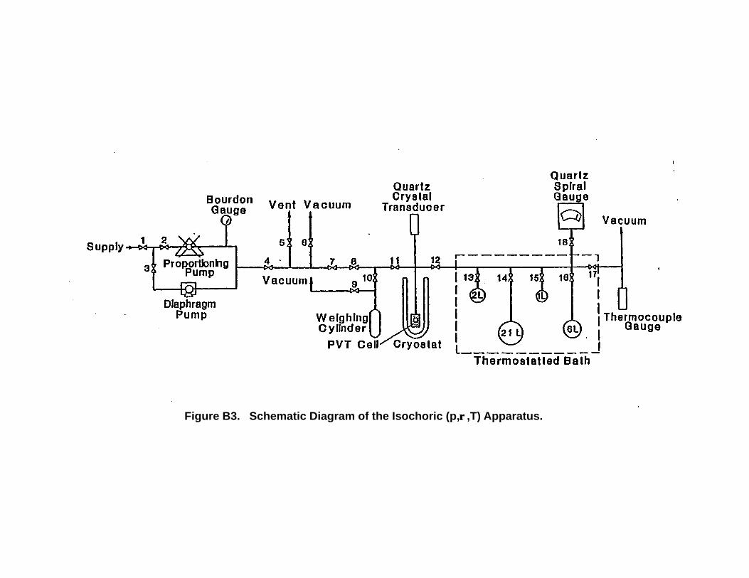
Figure B3. Schematic Diagram of the Isochoric (p,ρρ ,T) Apparatus.
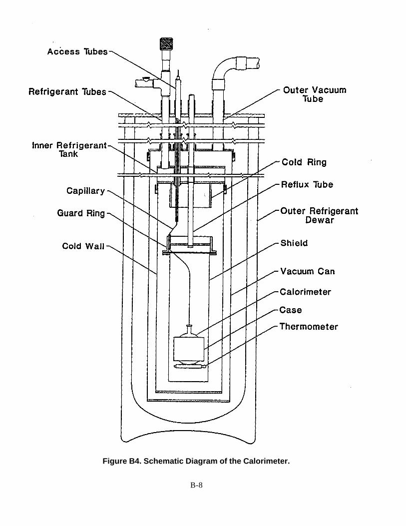
Figure B4. Schematic Diagram of the Calorimeter.
B-8

Figure B5. Schematic Diagram of Spherical Resonator Sound Speed
Apparatus
B-9
C-1
APPENDIX C:
ESTIMATES OF STATE-POINT UNCERTAINTIES
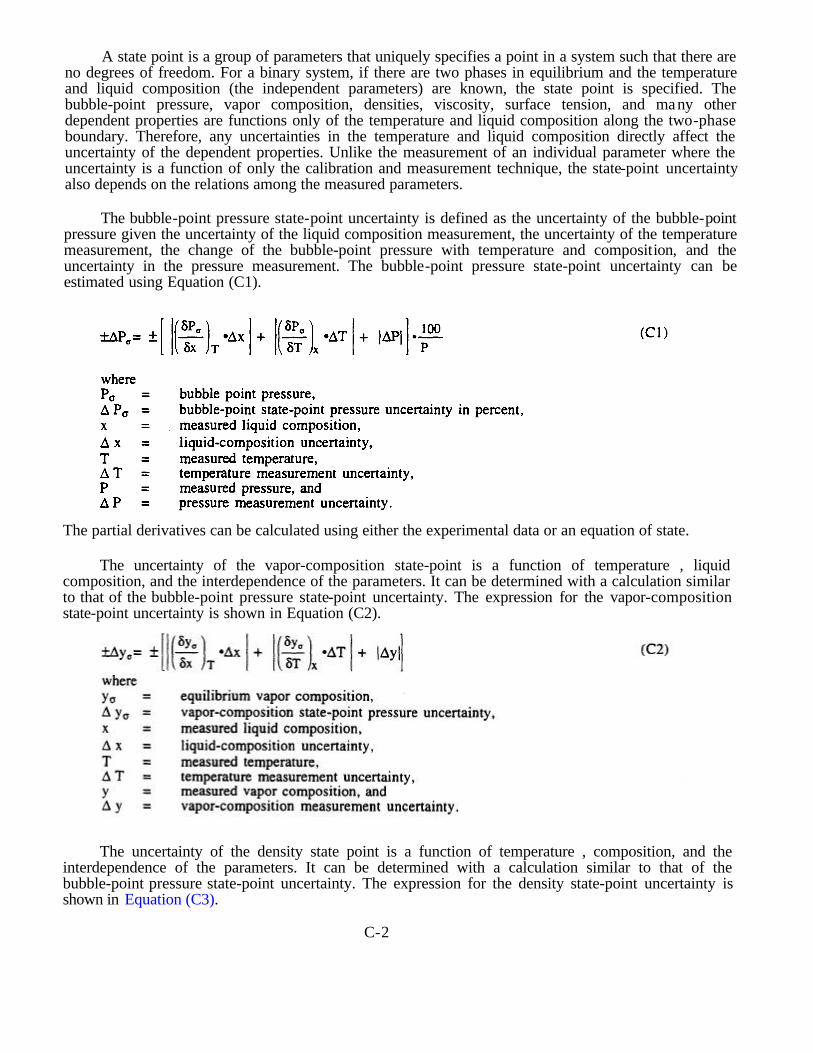
A state point is a group of parameters that uniquely specifies a point in a system such that there areno degrees of freedom. For a binary system, if there are two phases in equilibrium and the temperatureand liquid composition (the independent parameters) are known, the state point is specified. Thebubble-point pressure, vapor composition, densities, viscosity, surface tension, and many otherdependent properties are functions only of the temperature and liquid composition along the two-phaseboundary. Therefore, any uncertainties in the temperature and liquid composition directly affect theuncertainty of the dependent properties. Unlike the measurement of an individual parameter where theuncertainty is a function of only the calibration and measurement technique, the state-point uncertaintyalso depends on the relations among the measured parameters.
The bubble-point pressure state-point uncertainty is defined as the uncertainty of the bubble-pointpressure given the uncertainty of the liquid composition measurement, the uncertainty of the temperaturemeasurement, the change of the bubble-point pressure with temperature and composition, and theuncertainty in the pressure measurement. The bubble-point pressure state-point uncertainty can beestimated using Equation (C1).
The partial derivatives can be calculated using either the experimental data or an equation of state.
The uncertainty of the vapor-composition state-point is a function of temperature , liquidcomposition, and the interdependence of the parameters. It can be determined with a calculation similarto that of the bubble-point pressure state-point uncertainty. The expression for the vapor-compositionstate-point uncertainty is shown in Equation (C2).
The uncertainty of the density state point is a function of temperature , composition, and theinterdependence of the parameters. It can be determined with a calculation similar to that of thebubble-point pressure state-point uncertainty. The expression for the density state-point uncertainty isshown in Equation (C3).
C-2

C-3

APPENDIX D:
GAS CHROMATOGRAPH CALIBRATION PROCEDURES
D-1

D-2
The gas chromatograph calibration procedure involves six steps. The first step is the preparationof two or three standard mixtures for each system. These mixtures are used to determine which GCcolumn to use, to refine the calibration, and to check the sampling system for adsorption or mixingproblems. The number of mixtures needed is dependent on the type of GC column used to separatethe two components. A short-packed column usually requires two standard mixtures. A capillarycolumn or long-packed column requires three or more mixtures due to the complex behavior ofadsorption and desorption along the length of the column.
In the second step, the standard mixtures are used to determine which GC column best separatesthe two components and what are the appropriate settings on the GC. Table D1 summarizes the GCcolumns and settings used for each of the systems in this report.
In the third step of the procedure, density-versus-area data are obtained for the pure componentsfrom the GC. A specific volume is chosen for injection of the sample into the GC. This volume isfilled at different pressures of the pure fluid in a region where the virial equation for the pure fluidcan accurately predict the density. The pressure and temperature of the standard volume are recordedbefore each injection. The density of the injected gas is calculated from the virial equation of state.
The fourth step of the procedure characterizes any peak interaction or sample size dependenceby injecting different quantities of the standard mixtures into the GC. The same sample volume usedfor the pure fluids is filled to different pressures with the standard mixtures. The area-percent-versus-sample-size data are recorded.
The fifth step is determining the correct calibration equation to use with the calibration data. Forshort- packed columns the area percent of the GC peaks should be independent of the amount of thestandard mixture injected. The calibration equation for this type of column is based on combining thearea-versus-density data of the two pure components. Usually the area-versus-density relationshipsfor each of the pure components can be represented by a simple quadratic equation. The standardmixture data is used to optimize the fit and to check the accuracy of the equation.
A capillary column or long-packed column shows a dependence of area percent on the samplesize injected. The calibration equations for these systems are more complicated than for short-packedcolumns because they include a size dependence as well as a composition dependence that requiresall of the mixture and pure component data to be used in the fit. The procedure is more complicatedthan the procedure for a short-packed column, but is necessary in order to obtain accurate results.
The final step checks the sampling system for losses due to adsorption or inhomogeneoussampling. The apparatus is filled with one of the standard mixtures and several samples are analyzedusing the sampling system. The composition calculated from the GC should be the same as thecomposition of the standard mixture. If the composition is not the same as the standard mixture, oneof the components may be adsorbing to the walls of the sampling system or the sample is not wellmixed before it reaches the GC.
The GC calibration is only accurate within the peak area range of its calibration. If the sampleswithdrawn from the system are too large or too small, the calculated compositions will be in error.The size of the sample withdrawn from the apparatus must be adjusted to stay within the limits of thecalibration.

Table D1. Summary of the Gas Chromatograph Settings, the Separation Columns, and the Standard Reference MixturesUsed for Each Refrigerant System.