Theory-Based Causal Induction - cocosci.berkeley.educocosci.berkeley.edu/tom/papers/tbci.pdf ·...

Theory-Based Causal Induction

Thomas L. GriffithsUniversity of California, Berkeley

Joshua B. TenenbaumMassachusetts Institute of Technology

Inducing causal relationships from observations is a classic problem in scientific inference, statistics, andmachine learning. It is also a central part of human learning, and a task that people perform remarkablywell given its notorious difficulties. People can learn causal structure in various settings, from diverseforms of data: observations of the co-occurrence frequencies between causes and effects, interactionsbetween physical objects, or patterns of spatial or temporal coincidence. These different modes oflearning are typically thought of as distinct psychological processes and are rarely studied together, butat heart they present the same inductive challenge—identifying the unobservable mechanisms thatgenerate observable relations between variables, objects, or events, given only sparse and limited data.We present a computational-level analysis of this inductive problem and a framework for its solution,which allows us to model all these forms of causal learning in a common language. In this framework,causal induction is the product of domain-general statistical inference guided by domain-specific priorknowledge, in the form of an abstract causal theory. We identify 3 key aspects of abstract priorknowledge—the ontology of entities, properties, and relations that organizes a domain; the plausibilityof specific causal relationships; and the functional form of those relationships—and show how theyprovide the constraints that people need to induce useful causal models from sparse data.

Keywords: causal induction, intuitive theories, rational analysis, Bayesian modeling

In 1695, Sir Edmond Halley was computing the orbits of a setof comets for inclusion in Newton’s Principia Mathematica whenhe noticed a surprising regularity: The comets of 1531, 1607, and1682 took remarkably similar paths across the sky, and visited theEarth approximately 76 years apart. Newton had already shownthat comets should follow orbits corresponding to conic sections—parabolas, hyperbolas, and ellipses—although no elliptical orbitshad yet been observed. Halley inferred that the sightings of thesecomets were not three independent events, but three consequencesof a single common cause: a comet that had visited the Earth threetimes, travelling in an elliptical orbit. He went on to predict that itwould return along the same orbit in 1758. The comet returned as

predicted, and has continued to visit the Earth approximately every76 years since, providing a sensational confirmation of Newton’sphysics.

Halley’s discovery is an example of causal induction: inferringcausal structure from data. Explaining this discovery requiresappealing to two factors: abstract prior knowledge, in the form ofa causal theory, and statistical inference. The prior knowledge thatguided Halley was the mathematical theory of physics laid out byNewton. This theory identified the entities and properties relevantto understanding a physical system, formalizing notions such asvelocity and acceleration, and characterized the relations that canhold among these entities. Using this theory, Halley could generatea set of hypotheses about the causal structure responsible for hisastronomical observations: They could have been produced bythree different comets, each travelling in a parabolic orbit, or byone comet, travelling in an elliptical orbit. Choosing between thesehypotheses required the use of statistical inference. While Halleymade no formal computations of the probabilities involved, thesimilarity in the paths of the comets and the fixed interval betweenobservations convinced him that “it was highly probable, not to saydemonstrative, that these were but one and the same Comet” (fromthe Journal Book of the Royal Society, July 1696, reproduced inHughes, 1990, p. 353).

Causal induction is not just a problem faced by scientists. Thecapacity to reason about the causes of events is an essential part ofcognition from early in life, whether we are inferring the forcesinvolved in physical systems (e.g., Shultz, 1982b), the mentalstates of others (e.g., Perner, 1991), or the essential properties ofnatural kinds (e.g., S. A. Gelman & Wellman, 1991). Often, thesecausal relationships need to be inferred from data. Explaining howpeople make these inferences is not just a matter of explaininghow causation is identified from correlation, but of accounting for

Thomas L. Griffiths, Department of Psychology and Program in Cog-nitive Science, University of California, Berkeley; Joshua B. Tenenbaum,Department of Brain and Cognitive Sciences, Massachusetts Institute ofTechnology.

While completing this work, we were supported by the James S.McDonnell Causal Learning Research Collaborative, Air Force Office ofScientific Research Grants FA9550-07-1-0351 (to Thomas L. Griffiths)and FA9550-07-1-0075 (to Joshua B. Tenenbaum), and Army ResearchOffice MURI Grant W911NF-08-1-0242 (to Joshua B. Tenenbaum).

We thank Elizabeth Bonawitz, Tevye Krynski, Tania Lombrozo, Sour-abh Niyogi, Laura Schulz, and David Sobel for comments on the articleand related discussions, Marc Buehner for providing the data from Buehnerand Cheng (1997), and Hongjing Lu for providing a version of the datasetsconsidered by Perales and Shanks (2007) that included the valence of thecausal relationship. We are grateful to Elizabeth Bonawitz and AndreasStuhlmuller for their assistance in data collection.

Correspondence concerning this article should be addressed to ThomasL. Griffiths, Department of Psychology, 3210 Tolman Hall, MC 1650,University of California, Berkeley, CA 94720-1650. E-mail: [email protected]

Psychological Review © 2009 American Psychological Association2009, Vol. 116, No. 4, 661–716 0033-295X/09/$12.00 DOI: 10.1037/a0017201

661

how complex causal structure is inferred in the absence of (statis-tically significant) correlation. People can infer causal relation-ships from samples too small for any statistical test to producesignificant results (e.g., Gopnik, Sobel, Schulz, & Glymour, 2001)and solve problems like inferring hidden causal structure (e.g.,Kushnir, Gopnik, Schulz, & Danks, 2003) that still pose a majorchallenge for statisticians and computer scientists. Human causalinduction is not always on target: sometimes we miss causalconnections that would be most valuable to exploit, or see con-nections that do not in fact exist. Yet the successes stand out. Noconventional statistical recipe or computer learning algorithm cancompete with a young child’s capacity to discover the causalstructure underlying everyday experience—or at least, to comeclose enough to causal “ground truth” with knowledge that sup-ports such flexible prediction, planning, and action in the world.

In this article, we present a formal framework for explaininghow human causal learning works across a wide range of contextsand information sources. Our goal here is not a mechanistic ex-planation in terms of psychological processing steps or neuralmachinery. Rather we want to explain how human learners cansuccessfully infer such rich causal models of the world given thatthe data they observe are so sparse and limited. Our explanationsof human causal induction take the form of computational theories,in the sense introduced by Marr (1982) and pursued by Shepard(1987) and Anderson (1990), among others (see Oaksford &Chater, 1998): We identify the abstract computational problemaddressed by a cognitive capacity, derive an optimal solution tothat problem, and use that solution to explain human behavior.

In our analysis of the computational problem underlying every-day causal induction, the two factors of prior knowledge andstatistical inference that we identified in Halley’s famous discov-ery both play central roles. Prior knowledge, in the form of anabstract theory, generates hypotheses about the candidate causalmodels that can apply in a given situation. Principles of Bayesianinference generate weights for these hypotheses in light of ob-served data and thus predictions about which causal relations arelikely to hold, and which patterns of future events are likely to beobserved. To the extent that the prior knowledge is veridical—when people’s abstract intuitive theories reflect the way causalsystems in their environment tend to work—our rational frame-work explains how people’s inferences about the structure ofspecific causal systems can be correct, even given very little data.Yet our framework is not strictly normative: In cases where peoplehold the wrong abstract theories, rational statistical inference maylead them to incorrect beliefs about a novel system even givenextensive experience.

The idea that causal induction draws on prior knowledge is notnovel—it has been noted in many influential theories (e.g., Cheng,1997; Lien & Cheng, 2000), discussed in the context of rationalstatistical inference (Alloy & Tabachnik, 1984), and explored intwo separate research programs (Koslowski, 1996; Waldmann,1996; Waldmann, Hagmayer, & Blaisdell, 2006). However, pre-vious formal models have focused mostly on the effects of specificforms of prior knowledge, such as the plausibility of a causalrelationship, painting a relatively simple picture of the role thisknowledge plays in learning. Our contribution is a formal frame-work that provides a way to systematically identify the aspects ofprior knowledge that can influence causal induction, to describethis knowledge precisely, and to explain how it is combined with

rational mechanisms of statistical inference. We call this frame-work theory-based causal induction. We propose that three aspectsof prior knowledge are central in generating hypotheses for causalinduction—the ontology of entities, properties, and relations thatorganizes a domain; the plausibility of specific causal relation-ships; and the functional form of those relationships—and thatthese three aspects are the key constituents of people’s intuitivecausal theories. Mathematical models of causal induction in spe-cific settings can be derived by performing Bayesian inferenceover the hypothesis spaces generated by appropriate theories ofthis sort, and they illustrate how relatively complex interactionsbetween prior knowledge and data can emerge.

By viewing causal induction as the result of domain-generalstatistical inference guided by domain-specific causal theories, ourframework provides a unified account of a set of phenomena thathave traditionally been viewed as distinct. Different aspects ofcausal learning have tended to be explained in different ways.Theories of causal learning from contingency data, in which peo-ple are provided with information about the frequency with whichcause and effect co-occur and are asked to evaluate the underlyingrelationship, emphasize statistical learning from covariation be-tween cause and effect (e.g., Cheng, 1997; Jenkins & Ward, 1965;Shanks, 1995b). In contrast, analyses of learning about the causalrelationships that govern physical systems, such as simple ma-chines, tend to focus on the role of domain-specific knowledgeabout the nature of possible causal mechanisms (e.g., Bullock,Gelman, & Baillargeon, 1982; Shultz, 1982b). Finally, inferencesabout causal relationships based on spatial and temporal dimen-sions of dynamic events—most famously illustrated in Michotte’s(1963) classic studies of perceived causality in collisions—areoften viewed as the product of a modular, automatic perceptualmechanism, distinct from a general cognitive capacity for statisti-cal inference thought to underlie causal learning from contingencydata (e.g., Leslie, 1986; Schlottmann & Shanks, 1992).

From the perspective of theory-based causal induction, theseapparently disparate phenomena are not discrete cases requiringseparate explanations but rather points on a continuum, where thestrength of the constraints provided by prior knowledge graduallyincreases, and the amount of information required in order to makea causal inference decreases accordingly. Standard experiments oncausal induction from covariational data tap into relatively weakprior knowledge and hence require a relatively large number ofexperienced events (typically, tens of data points) for learners toreach confident causal conclusions. Causal learning in simplephysical systems draws on richer knowledge about causal mech-anisms, allowing confident causal inferences from only a handfulof examples. When even richer (if implicit) knowledge about thespatiotemporal dynamics of physical interactions is involved, as instandard cases of perceptual causality, confident inferences can bemade from just a single observed event—a “suspicious coinci-dence”—with the appropriate spatiotemporal structure.

The plan of the article is as follows. In the next section, wesummarize previous work illustrating how different aspects ofprior knowledge can influence causal learning. We then discuss thegoals of a computational-level analysis of causal induction, focus-ing on a description of the central inductive problems to be solvedby the learner. This description introduces causal graphical mod-els, a formalism for representing and reasoning about causal rela-tionships which has been the basis for previous accounts of human

662 GRIFFITHS AND TENENBAUM

causal induction, but which crucially does not have the ability toexpress the forms of abstract prior knowledge that guide humancausal learning along such different trajectories in different do-mains and contexts. We then introduce our framework of theory-based causal induction, building on the foundation of causal graph-ical models but making explicit the structure and function of thelearner’s prior knowledge. The bulk of the article consists of theapplication of this framework to the settings mentioned above:causal induction from contingency data, learning about the prop-erties of physical systems, and inferring causal relationships fromcoincidences in space and time. In considering these phenomena,we focus on the importance of the two key components of ourapproach—statistical inference and prior knowledge expressed inthe form of a causal theory—in explaining how people can learnabout causal relationships from limited data.

How Does Prior Knowledge Influence Causal Induction?

The study of causal induction has a long history, in both phi-losophy (e.g., Hume, 1739/1978) and psychology (e.g., Inhelder &Piaget, 1958). Detailed reviews of some of this history are pro-vided by Shultz (1982b; Shultz & Kestenbaum, 1985) and White(1990, 1995). This history is marked by a tension between statis-tical learning and abstract prior knowledge about causality asaccounts of human causal induction. Psychological theories aboutcausal induction have tended to emphasize one of these two factorsover the other (Cheng, 1997; Newsome, 2003; Shultz, 1982b): Inthe tradition of Hume (1739/1978), covariation-based approachescharacterize human causal induction as the consequence of adomain-general statistical sensitivity to covariation between causeand effect (e.g., Cheng & Novick, 1990, 1992; Shanks & Dickin-son, 1987), whereas, in a tradition often traced to Kant (1781/1964;see Shultz, 1982b, for an account of the connection), mechanism-based approaches focus on the role of prior knowledge about themechanisms by which causal force can be transferred (e.g., Ahn &Kalish, 2000; Shultz, 1982b; White, 1995).

Recently, explanations of human causal learning have begun toexplore a middle ground between these positions, looking at howmechanism knowledge might influence learning from covariationbetween cause and effect (e.g., Lagnado & Sloman, 2004;Lagnado, Waldmann, Hagmayer, & Sloman, 2007; Waldmann,1996; Waldmann et al., 2006). These accounts are based on a rangeof results indicating the importance of both of these factors. Theanalysis that we present in this article can be viewed in part as anattempt to develop a formal framework that can capture the kind ofknowledge needed to explain these effects, providing the toolsrequired to define computational models of this “knowledge-based” approach to causal induction (Waldmann, 1996). As a firststep toward developing such a framework, we need to identifyexactly what aspects of prior knowledge are relevant to causalinduction. In this section, we briefly review work that has exploredthis question, using the example of Halley’s discovery for illus-tration. Following this example, we divide the kind of prior knowl-edge that is relevant to causal induction into three categories:information about the types of entities, properties, and relationsthat arise in a domain (the ontology); constraints on the plausiblerelations among these entities; and constraints on the functionalform of such relations.1

Ontology

Newton’s theory of physics picked out the critical variables forthinking about the motion of objects—their mass, velocity, andacceleration. The question of how entities are differentiated on thebasis of their causal properties has been thoroughly explored indevelopmental psychology, through consideration of the ontolog-ical commitments reflected in the behavior of infants and youngchildren. Both infants and young children have strong expectationsabout the behavior of physical objects, and these expectations arequite different from those for intentional agents (Saxe, Tenen-baum, & Carey, 2005; Shultz, 1982a; Spelke, Phillips, & Wood-ward, 1995). Similarly, children have different expectations aboutthe properties of biological and nonbiological entities (e.g.,Springer & Keil, 1991). Gopnik et al. (2001) have shown thatchildren use the causal properties of entities to determine whetherthey belong to a novel type—objects that differed in appearancebut both activated a “detector” were more likely to both be con-sidered “blickets” than objects with similar appearance that dif-fered in their causal properties.

Research with adults has also explored how the types of entitiesinfluence causal inferences. For example, Lien and Cheng (2000)conducted several experiments examining the circumstances underwhich causal properties are generalized across the members of acategory. In a typical experiment, people learned about the ten-dency of 15 chemicals to produce blooming in a plant. Thechemicals could be divided into groups on the basis of their colorand shape. Lien and Cheng explored how people used informationabout color and shape, which provided a basis for identifyingdifferent types of chemicals in causal learning. Their conclusionwas that people used these types in learning causal relationships:People formed the generalization that chemicals of the type thatmaximized the strength of the resulting relationship were thosethat caused the plant to bloom. In related work, Waldmann andHagmayer (2006) examined how intuitive theories influencewhether previously learned categories are transferred to novelcausal learning problems. Tenenbaum and Niyogi (2003) alsoshowed that people spontaneously organize objects into types onthe basis of their causal properties, forming abstract categories ofschematic blocks that cause one another to light up in a computersimulation, and Kemp, Goodman, and Tenenbaum (2007) showedthat such categories could carry with them expectations about thestrength of causal relationships.

Plausible Relations

Knowledge of the types of entities in a domain can provide quitespecific information about the plausibility of causal relationships.For example, Newton precisely laid out the kinds of forces bywhich the properties of one object can influence those of another.Explorations of how plausibility influences causal induction have

1 Although we refer to expectations about ontologies, plausible relations,and functional form as prior knowledge, we mean this to be interpreted asindicating that the knowledge is available prior to a specific instance ofcausal induction. We are not claiming that this knowledge is innate, andanticipate that in almost all cases it is acquired through experience with theworld and in particular through other instances of causal induction, a pointthat we return to in our discussion of learning causal theories.

663THEORY-BASED CAUSAL INDUCTION

examined mainly how children learn about the structure of phys-ical systems (e.g., Shultz, 1982b), although even accounts ofcausal induction from contingency data that emphasize the impor-tance of covariation between cause and effect recognize a role fortop-down knowledge (e.g., Cheng, 1993, 1997). In one classicstudy, Shultz (1982b) demonstrated that young children havestrong expectations about the plausibility of different kinds ofcausal relationships, in part derived from their experience with theproperties of these objects in the course of the experiment. Forexample, he found that children used the knowledge that a lamp ismore likely than a fan to produce a spot of light, that a fan is morelikely than a tuning fork to blow out a candle, and that a tuningfork is more likely than a lamp to produce resonance in a box.

On the basis of examples like those provided by Shultz (1982b),several authors have equated the plausibility of a causal relation-ship with the existence of a potential mechanism by which thecause could influence the effect (e.g., Ahn & Kalish, 2000;Schlottmann, 1999). Koslowski and colleagues (Koslowski, 1996;Koslowski & Okagaki, 1986; Koslowski, Okagaki, Lorenz, &Umbach, 1989) have conducted a series of experiments investi-gating this claim, finding that people consider causal relationshipsmore plausible when supplied with a potential mechanism and lessplausible when the most likely mechanisms are ruled out.

Recent work examining causal learning in adults has also notedthe importance of prior expectations about the direction of causalrelationships, particularly when people are simultaneously learningabout multiple relationships. Waldmann and colleagues (Wald-mann, 1996, 2000; Waldmann & Holyoak, 1992; Waldmann,Holyoak, & Fratianne, 1995) have conducted a number of studiesthat suggest that people’s expectations about the causal structureamong a set of variables can determine how covariational evidenceaffects their beliefs. For example, Waldman (2000) gave peopleinformation that suggested that the relationship among a set ofvariables was either a “common cause” relationship, with onevariable causing several others, or a “common effect” relationship,with several variables all producing a single effect. People’s be-liefs about the underlying causal structure influence their interpre-tation of the pattern of covariation among the variables: Only thosewho believed in the common effect structure took into accountcompetition between causes when evaluating their strength.

Functional Form

In physics, the functional form of causal relationships, such ashow the velocity of one object depends on its mass and the massand velocity of another object with which it collides, can be laidout precisely. The knowledge that guides most causal inferences isless precise, but even in the most basic cases of causal inductionwe draw on expectations as to whether the effects of one variableon another are positive or negative, whether multiple causes inter-act or are independent, and what type of events (binary, continu-ous, or rates) are relevant to evaluating causal relationships(Cheng, 1997; Novick & Cheng, 2004).

One setting in which questions about functional form havearisen explicitly is in examining how causes should be assumed tocombine. Many theories of animal learning assume that multiplecauses of a single effect combine additively, each making a con-stant contribution to the effect (e.g., Rescorla & Wagner, 1972). Anumber of researchers, including Shanks, Wasserman, and their

colleagues, have advocated these linear models as accounts ofhuman causal learning (e.g., Lopez, Cobos, Cano, & Shanks, 1998;Shanks, 1995a, 1995b; Shanks & Dickinson, 1987; Wasserman,Elek, Chatlosh, & Baker, 1993). However, whether this assump-tion is appropriate for modeling human judgments seems to beaffected by people’s beliefs about what aspect of the causesproduces the effect. Waldmann (2007) presented a study in whichparticipants were told about a hypothetical experiment that foundthat drinking a yellow liquid increased the heart rate of animals by3 points, while drinking a blue liquid increased the heart rate by 7points. The participants were asked to predict the consequences ofdrinking a mixture of the two liquids. The results depended uponwhether the participants were told that the effect of the drink wasa consequence of its taste, or of its strength. More people producedpredictions consistent with a weighted average of the effects ifthey believed the effect was modulated by strength, for which alinear functional form is more appropriate. Recent work has alsoshown that the magnitude of some effects that assume additivity isaffected by the extent to which people believe causes combineadditively (Beckers, De Houwer, Pineno, & Miller, 2005; Lovi-bond, Been, Mitchell, Bouton, & Frohart, 2003).

Perhaps the most comprehensive attempt to characterize thepossible ways in which causes could combine is that of Kelley(1973), who suggested that causal induction from small numbersof observations may be guided by causal schemas. Kelley distin-guished between generative and preventive causes, and he identi-fied three schemas describing the interaction between generativecauses: multiple sufficient causes, multiple necessary causes, andcompensatory causes. Under the multiple sufficient causesschema, the effect occurs in the presence of any one of the causes(the equivalent of a logical OR function). In the multiple necessarycauses schema, the effect occurs only if all of the causes arepresent (the equivalent of a logical AND function). In the com-pensatory causes schema, increasing the strength of each causeincreases the tendency for the effect to be expressed. All of theseschemas constitute different assertions about the functional formof the relationship between cause and effect, and knowing whichof these schemas is relevant in a particular situation can facilitateevaluating whether a particular causal relationship exists.

The functional form of causal relationships becomes most im-portant when dealing with causal inferences in physical systems,where the ways in which one object influences another can bequite complex. Developmental psychologists have extensively in-vestigated how well children understand the functional relation-ships that hold in physical systems. Shultz and Kestenbaum (1985)provided a review of some of this work. One interesting exampleof this project is provided by Zelazo and Shultz (1989), whoinvestigated whether children understood the different functionalrelationships between the potency of a cause and the resistance ofthe effect in two systems: a balance beam, where one object wasweighed against another, and a ramp, where one object slid downto displace another. For the balance beam, the magnitude of theeffect depends upon the difference in the masses of the twoobjects, whereas for the ramp, it depends upon the ratio. Zelazoand Shultz (1989) found that although adults were sensitive to thisdifference, 5-year-olds tended to use a single functional form forboth systems.

The functional form of a causal relationship can also determinethe temporal coupling between cause and effect. The time between


the occurrence of a potential cause and the occurrence of an effectis a critical variable in many instances of causal induction. Severalstudies have explored covariation and temporal proximity as cuesto causality in children, typically finding that the event that im-mediately precedes an effect is most likely to be perceived as thecause, even if there is covariational evidence to the contrary (e.g.,Shultz, Fisher, Pratt, & Rulf, 1986). Hagmayer and Waldmann(2002) presented an elegant series of studies that showed thatdifferent assumptions about the delay between cause and effectcould lead to different interpretation of the same set of events,determining which events were assumed to be related. Similarphenomena have recently been investigated in detail by Lagnadoand Sloman (2006) and Buehner and colleagues (Buehner & May,2002, 2003; Greville & Buehner, 2007). Finally, Anderson (1990)provided a computational analysis of data involving the interactionbetween spatial separation and temporal contiguity in causal in-duction.

Summary

The three aspects of prior knowledge identified in this sectioncan support strong expectations about possible causal relation-ships. Having an ontology, knowing the plausibility of relation-ships among the entities identified within that ontology, and know-ing the functional form of those relationships provides informationthat makes it possible to generalize about the causal relationshipsamong completely new variables. The research we have summa-rized in this section makes a compelling case for an influence ofprior knowledge on causal induction but raises the question ofexactly how this knowledge should be combined with the evidenceprovided by the data observed by learners. Answering this questionis the project undertaken in the remainder of the article. Our nextstep toward obtaining an answer is to understand the computa-tional problem underlying causal induction, which is the focus ofthe next section.

A Computational-Level Analysis of Causal Induction

The aim of this article is to provide a computational-levelanalysis of causal induction, in the sense introduced by Marr(1982). This section begins with a discussion of what such ananalysis means, clarifying our motivation and methodology. Wethen turn to the question of how to formulate the computationalproblem underlying causal induction. Our formulation of thisproblem makes use of causal graphical models, a formalism forrepresenting, reasoning with, and learning about causal relation-ships developed in computer science and statistics (Pearl, 2000;Spirtes, Glymour, & Scheines, 1993). We introduce this formalismand use it to clearly state the problem faced by causal learners. Wethen consider existing rational solutions to this problem, arguingthat while they feature one of the two factors that are necessary toexplain human causal induction—statistical inference—they donot incorporate the kind of prior knowledge described in theprevious section. Reflecting upon the nature of this knowledgeleads us to argue that a level of representation that goes beyondcausal graphical models will be required.

Analyzing Causal Induction at the Computational Level

Marr (1982) distinguished between three levels at which aninformation processing system can be analyzed: the levels of

computational theory, representation and algorithm, and hardwareimplementation. Analyses at the first of these levels answer thequestion “What is the goal of the computation, why is it appro-priate, and what is the logic of the strategy by which it can becarried out?” (Marr, 1982, p. 25). This is a question about theabstract problem that the information processing system is tryingto solve and what solutions to that problem might look like. Onepart of a computational-level analysis is thus considering the formof rational solutions to a problem faced by the learner, a strategythat is also reflected in Shepard’s (1987) search for universals lawsof cognition—laws that must hold true for any information-processing system due to the structure of the problem beingsolved—and Anderson’s (1990) formulation of rational analysis.

In the context of causal induction, a computational-level anal-ysis seeks to identify the abstract problem being solved whenpeople are learning about causal relationships and to understandthe logic that makes it possible to solve this problem. Since ouraim is to provide a unifying account of causal induction across arange of settings, we want to define the underlying computationalproblem in as broad a way as possible, highlighting the fact that asingle solution can be applied across these domains. A majorchallenge of this approach is finding a formal framework that canprovide a solution to the underlying computational problem, com-pounded by the fact that we want more than just any solution: Wewant a solution that is optimal for the problem being posed.

Developing an account of causal induction that is an optimalsolution to the underlying computational problem is attractive notjust as a unifying account, but as a way of answering three kindsof questions about human cognition. The first kind of question isa “How possibly?” question: How could people possibly solve theproblem of inferring causal relationships from observational data?Many aspects of human learning, including causal induction, seemfar better than that of any automated systems. To repeat an exam-ple from the introduction, it is commonplace for people to drawcorrect conclusions about causal relationships from far less datathan we might need to do a statistical test. Understanding how wemight explain such inferences in rational terms helps us understandhow it is that people are so good at them, and what factors—suchas domain knowledge—play a role in this success.

The second kind of question we can answer using this kind ofanalysis is a “How should it be done?” question: Given thecomputational problems that people face, what should they bedoing to solve those problems? Optimal solutions tell us somethingabout the properties that we might expect to see in the behavior ofintelligent organisms, and can thus tell us which aspects of thatbehavior might be purely a consequence of the nature of theproblems being solved. This kind of strategy is common in visionscience, where “ideal observer” models have helped reveal howmuch of human perception might be explained as an optimalresponse to the structure of the environment (Yuille & Kersten,2006). In the case of causal induction, a critical issue is combiningstatistical evidence with prior knowledge, and a rational accountcan indicate how this should be done, and what the consequencesshould be for the inferences that people make. Although researchin judgment and decision-making has illustrated that people oftendeviate from the predictions of rational models (e.g., Tversky &Kahneman, 1974), the revelations that this work has made aboutthe psychological mechanisms involved were partially made pos-sible by the existence of a well-developed account of how a


rational agent should make decisions. For other complex problemssuch as causal induction, we are only just beginning to developthese rational accounts, and understanding what people should dowhen making causal inferences will be a valuable tool in deter-mining how people actually solve this problem.

Finally, a third, related, question we can answer is a “What isnecessary?” question: What knowledge or other constraints onhypotheses would an ideal learner need in order to reach the sameconclusions as people? Since an ideal learner makes the best use ofthe available data, the answer to this question places a lower boundon the kind of constraints that human learners might use. Under-standing the impact of different kinds of prior knowledge on causalinduction by analyzing their effects on an ideal learner gives us away to predict the role that these kinds of knowledge might play inhuman causal induction.

Answering these three questions requires not just defining aproblem and deriving a solution, but arguing that this problem andsolution connect to human causal learning. This connection can beestablished only by comparing the predictions of models devel-oped within our formal framework to the results of experimentswith human participants. The empirical results that will be relevantto this argument are those that are framed at the same level ofabstraction as our analysis: results that indicate what conclusionspeople reach given particular data. As a consequence, we focusmainly on static measurements of beliefs about causal relation-ships, rather than capturing the dynamics of human learning,although we have explored this topic in the past (Danks, Griffiths,& Tenenbaum, 2003) and view it as an important direction forfuture research. The goal of our models is to produce the sameconclusions from the same data, and our framework will be suc-cessful if it allows us to define models that incorporate the kindsof knowledge that make this possible.

In pursuing a computational-level analysis, we are not trying tomake claims about the other levels at which causal induction mightbe analyzed. In particular, we are not asserting that particularrepresentations or algorithms are necessary, or making other com-mitments as to the mechanisms or the psychological processesinvolved. Marr (1982) argued that different levels of analysis willprovide constraints on one another, with the computational levelindicating what kinds of representations and algorithms will beappropriate for solving a problem. In the context of causal induc-tion, we anticipate that many different psychological mechanismscould result in behavior similar to the predictions made by specificmodels we consider, with associative learning, heuristics, or ex-plicit hypothesis testing being good strategies for individual tasks,and we briefly outline some possible psychological mechanisms inthe Discussion. Our general aim, however, is to provide a unifyingaccount at the more abstract level of the underlying problem andits solution, ultimately helping to explain why particular represen-tations and algorithms might be appropriate in a particular task.

Finally, our aim of providing a computational-level account ofcausal induction also influences the kinds of models that we usefor comparison. In this article, our emphasis is on comparison ofthe predictions of our account to those of other rational models.These models all use the same formal ideas and operate at the samelevel of analysis, but they differ in their assumptions about theknowledge that informs causal induction or the nature of statisticallearning. Comparison with these other rational models thus helpsto highlight which components of our framework are relevant to

explaining behavior on a given task. We do not doubt that it ispossible to define better models of specific tasks, since presumablyan accurate model of the actual mechanisms people use to solvethese problems will make better predictions than the abstract kindof analyses obtained from our framework. Ultimately, we see thekey criterion for the success of our approach to be its usefulness incapturing the effects of prior knowledge on causal induction acrossa wide range of settings, and it is this criterion that we have inmind when we evaluate the performance of individual models. Inthis way, we expect that our framework will be evaluated in thesame fashion as other general approaches that can be used todefine a variety of computational models, such as parallel distrib-uted processing (e.g., McClelland & Rumelhart, 1986) or produc-tion systems (e.g., Anderson, 1993).

Causal Graphical Models

Having introduced our motivation and methodology, we nowturn to the question of how to formulate the computational prob-lem posed by causal induction. We will do this using causalgraphical models, also known as Bayesian networks or Bayes nets.Causal graphical models have recently begun to be used in psy-chological accounts of causality (e.g., Danks & McKenzie, 2009;Glymour, 1998, 2001; Gopnik et al., 2004; Griffiths & Tenen-baum, 2005; Lagnado & Sloman, 2002; Lu, Yuille, Liljeholm,Cheng, & Holyoak, 2006, 2007, 2008; Rehder, 2003; Steyvers,Tenenbaum, Wagenmakers, & Blum, 2003; Tenenbaum & Grif-fiths, 2001, 2003; Waldmann & Martignon, 1998). In this article,we highlight only the elements of causal graphical models that arerelevant to our account. More detailed introductions are providedby Pearl (2000), Heckerman (1998), Glymour (2001), and Sloman(2005).

A causal graphical model has three components: a set of vari-ables, a causal structure defined upon those variables, and a set ofassumptions about the functional form of the relationships indi-cated by this structure. The variables are represented by nodes ina graph. These nodes are connected by arrows, indicating thedirection of causal dependencies among the variables. Assump-tions about the functional form of causal relationships make itpossible to use this graphical structure to reason about the proba-bilities of different kinds of events. The functional form defines aprobability distribution for each variable conditioned on its causes,which is referred to as the parameterization of the nodes.

Causal graphical models can be used to compute the probabilityof observing particular values for the variables and the conse-quences of interventions. An intervention is an event in which avariable is forced to hold a value, independent of any othervariables on which it might depend. Following Pearl (2000), wedenote intervention that sets a variable X to value x with do(x), andin general use uppercase letters to indicate variables and lowercaseletters to indicate their values. Probabilistic inference on a modi-fied graph, in which incoming edges to X are removed, can be usedto assess the consequences of intervening on X (Pearl, 2000;Spirtes et al., 1993).

The Computational Problem and Existing Solutions

Causal graphical models provide us with the tools to give aprecise definition of the computational problem underlying causal


induction. We take the problem of causal induction as that ofidentifying the causal graphical model—including both structureand parameters—responsible for generating the observed data D.This problem has been extensively explored in the literature oncausal graphical models in computer science and statistics, and itis typically divided into two parts (e.g., Griffiths & Tenenbaum,2005; Heckerman, 1998): structure learning and parameter estima-tion. We discuss these parts in turn, highlighting connections toexisting proposals about human causal induction.

Structure learning. Learning the causal structure that relates alarge number of variables is a difficult computational problem, asthe number of possible structures increases exponentially with thenumber of variables. Research in computer science and statisticshas focused on two strategies for solving this problem. Constraint-based algorithms attempt to identify causal structure on the basisof the patterns of dependency exhibited by a set of variables,whereas Bayesian methods evaluate the probability that a partic-ular structure generated the observed data.

Constraint-based algorithms for structure learning (e.g., Pearl,2000; Spirtes et al., 1993) proceed in two steps. First, standardstatistical tests such as Pearson’s �2 test are used to identify whichvariables are dependent and independent. Since different causalstructures should result in different patterns of dependency amongvariables, the observed dependencies provide constraints on the setof possible causal structures. The second step of the algorithmsidentifies this set, reasoning deductively from the pattern of de-pendencies. The result is one or more causal structures that areconsistent with the dependencies exhibited by the data. By notmaking any commitments about the consequences of causal rela-tionships other than statistical dependency, constraint-based algo-rithms provide a general-purpose tool for causal induction that canbe applied easily across many domains. This generality is part ofthe appeal of these algorithms as psychological theories, as theyprovide a way to explain the acquisition of causal knowledgewithout recourse to domain-specific mechanisms (e.g., Gopnik &Glymour, 2002; Gopnik et al., 2004).

The Bayesian approach to structure learning (Cooper & Hers-kovits, 1992; see Heckerman, 1998) treats causal induction as aspecial case of the more general statistical problem of identifyingthe statistical model most likely to have generated observed data.Bayesian inference provides a solution to this problem. The heartof this solution is Bayes’ rule, which can be used to evaluate theprobability that a hypothetical model h was responsible for gen-erating data D. The posterior distribution, P(h�D), is evaluated bycombining prior beliefs about the probability that h might generateany data, encoded in the distribution P(h), with the probability ofD under the model h, P(D�h), typically referred to as the likelihood.Bayes’ rule stipulates how these probabilities should be combined,giving

P�h�D� �P�D�h�P�h�

�h��HP�D�h��P�h��, (1)

where H is the hypothesis space, the set of all models that couldpossibly have produced D.

As with any Bayesian inference, this approach requires speci-fying a prior probability and a likelihood for every hypothesiswithin a hypothesis space, H. In typical applications of thismethod, H consists of all directed graphs defined over the available

variables. The data D consist of the values that those variablesassume as the result of observation and intervention. StandardBayesian structure-learning algorithms define P(D�h) in a way thatmakes very weak assumptions about the functional form of therelationship between causes and effects. A separate parameter isused to express the probability of the effect for each configurationof its causes, meaning that the causes can have essentially any kindof influence on the effect—generative or preventive, large orsmall—and can combine in any imaginable way. P(D�h) is evalu-ated by defining a distribution over these parameters, and thenintegrating over the specific values the parameters take on (e.g.,Cooper & Herskovits, 1992). This makes it possible to computethe probability of the data given a particular graphical structurewithout committing to a particular choice of parameter values. Theprior over graph structures, P(h), is typically either uniform (giv-ing equal probability to all graphs), or gives lower probability tomore complex structures. Algorithms that use these principlesdiffer in whether they then proceed by searching the space ofstructures to find that with the highest posterior probability (Fried-man, 1997), or evaluate particular causal relationships by integrat-ing over the posterior distribution over graphs (Friedman & Koller,2000). Tenenbaum and Griffiths (2001; Griffiths & Tenenbaum,2005) developed a model of human causal induction based on theprinciples of Bayesian structure learning, which we discuss inmore detail later in the article.

Parameter estimation. Parameter estimation assumes a fixedcausal structure and aims to identify the parameters that specify theprobability of a variable given the values of the variables thatinfluence it. The simplest way to parameterize a causal graphicalmodel is to use a separate parameter for the probability of eachvalue of a variable given the values of its causes—something thatwe refer to as the generic parameterization. This generic parame-terization is the one typically used in Bayesian structure learning incomputer science, as discussed above. An alternative is to make astronger set of assumptions about the way in which causes com-bine to produce their effects. One such set of assumptions yieldsthe noisy-OR function, which is widely used in computer scienceand statistics (Pearl, 1988) and is a key part of a prominent modelof human causal induction (Cheng, 1997).

The noisy-OR function results from a natural set of assumptionsabout the relationship between cause and effect: that causes aregenerative, increasing the probability of the effect, that the effectoccurs in the absence of any causes with a constant probability w0,that each cause produces the effect with a constant probability wi,and that the opportunities for the causes to produce the effect areindependent (Cheng, 1997). For example, if we had an effectvariable E and a cause variable C, then the conditional probabilityof E given C would be

P�e��c; w0, w1� � 1 � �1 � w0��1 � w1�c, (2)

where w1 is a parameter associated with the strength of C and ctakes on values c� � 1 in the presence of the cause or c� � 0 inits absence. This expression gives w0 for the probability of E in theabsence of C, and w0 � w1 – w0w1 for the probability of E in thepresence of C. This parameterization is called a noisy-OR becauseif w0 and w1 are both 1, Equation 2 reduces to the logical ORfunction: The effect occurs if and only if either some backgroundfactor or C is present. With w0 and w1 in the range [0, 1] itgeneralizes this function to allow probabilistic causal relationships.


If E had multiple parents X1, . . . , Xn, we could associate a separatestrength wi with each parent, and the noisy-OR parameterizationwould give

P�e��x1, . . . , xn; w0, w1, . . . , wn� � 1 � �1 � w0��i

�1 � wi�xi,

(3)

where again xi � 1 if Xi is present, and 0 if Xi is absent.A simple solution to the problem of estimating the parameters of

a causal graphical model is to use maximum-likelihood estimation,choosing the values of the parameters that maximize the probabil-ity of the observed data. For the case of the noisy-OR function witha single cause, the maximum-likelihood estimate of w1 is

power �P�e��c�� P�e��c��

1 � P�e��c��, (4)

where P(e��c�) is the empirical conditional probability of theeffect given the presence of the cause. We have labeled thisquantity power as it corresponds to Cheng’s (1997) definition ofcausal power, proposed as a rational model of human causalinduction. Glymour (1998) pointed out that the assumptions Cheng(1997) used in deriving this model are equivalent to those under-lying the noisy-OR parameterization, and Tenenbaum and Grif-fiths (2001; Griffiths & Tenenbaum, 2005) showed that causalpower is a maximum-likelihood estimator of w1.

The numerator of Equation 4 has also been proposed in its ownright as a model of human causal induction, being known as �P.This quantity,

�P � P�e��c�� P�e��c��,

reflects the change in the probability of the effect occurring as aconsequence of the occurrence of the cause. This measure was firstsuggested by Jenkins and Ward (1965), was subsequently exploredby Allan (1980, 1993; Allan & Jenkins, 1983), and has appeared invarious forms in both psychology and philosophy (Cheng &Holyoak, 1995; Cheng & Novick, 1990, 1992; Melz, Cheng,Holyoak, & Waldmann, 1993; Salmon, 1980). �P can also beshown to be a rational solution to the problem of estimating thestrength of a causal relationship, assuming that causes combinelinearly (Griffiths & Tenenbaum, 2005; Tenenbaum & Griffiths,2001).

Two Challenges for a Formal Framework

This brief survey of existing methods for solving the problem ofidentifying the causal graphical model that generated observeddata—and corresponding rational models of human causal induc-tion—highlights two challenges for the kind of formal frameworkwe aim to develop. First, this framework should naturally capturethe effects of knowledge on causal induction. Existing approachesmake either weak or generic assumptions about the nature of theknowledge that people use in evaluating causal relationships andare consequently limited in their ability to account for the effectsof ontology, plausibility, and functional form outlined in the pre-vious section. Second, the framework should be broad enough toencompass learning of both causal structure and the parametersthat describe a given causal relationship. We now discuss these

issues in turn, arguing that both can be addressed by adopting amore general Bayesian framework.

Capturing the effects of prior knowledge. The approaches tostructure learning and parameter estimation outlined above allmake either weak (in the case of structure learning) or general-purpose (in the case of parameter estimation) assumptions aboutthe nature of causal relationships. These assumptions are incom-patible with the richness of human knowledge about causal rela-tionships and the corresponding flexibility of human causal induc-tion exhibited in the examples discussed in the previous section. Inpart, this is a consequence of the context in which these approacheswere developed. In statistics and computer science, developingalgorithms that make minimal assumptions about the nature ofcausal relationships maximizes the number of settings in whichthose algorithms can be used. Psychological models of causalinduction have justified making general-purpose assumptionsabout the nature of causal relationships through the expectationthat it will be relatively straightforward to integrate the effects ofprior knowledge into the resulting models. For example, Cheng(1997, p. 370) stated:

The assumption that causal induction and the influence of domain-specific prior causal knowledge are separable processes is justified bynumerous experiments in which the influence of such knowledge canbe largely ignored . . . . The results of these experiments demonstratethat the induction component can indeed operate independently ofprior causal knowledge.

In the few cases where formal accounts of the integration of priorknowledge and data have been explored (e.g., Alloy & Tabachnik,1984; Lien & Cheng, 2000), these accounts have focused on justone aspect of prior knowledge, such as the plausibility of causalrelationships or the level of the ontology at which those relation-ships should be represented.

Constraint-based structure-learning algorithms are particularlylimited in their use of prior knowledge.2 Again, this is partly bydesign, being a result of the data-driven, bottom-up approach tocausal induction that these algorithms instantiate in a particularlyclear way. As these algorithms are defined, they use only a weakform of prior knowledge—the knowledge that particular causalrelationships do or do not exist (e.g., Spirtes et al., 1993). They donot use prior knowledge concerning the underlying ontology, theplausibility of relationships, or their functional form. This insen-sitivity to prior knowledge has previously been pointed out bysome critics of constraint-based algorithms in computer scienceand statistics (Humphreys & Freedman, 1996; Korb & Wallace,1997). Prior knowledge provides essential guidance to humaninferences, making it possible to infer causal relationships fromvery small samples. Without it, constraint-based algorithms re-quire relatively large amounts of data in order to detect a causalrelationship— enough to obtain statistically significant resultsfrom a statistical significance test.

2 It might not be impossible to develop a more global constraint-basedframework for causal induction, defined over richer representations of priorknowledge and integrating both bottom-up and top-down information in amore holistic style of inference. However, this would be a major departurefrom how constraint-based approaches have traditionally been developed(Spirtes et al., 1993; Glymour, 2001).


The need for relatively large amounts of data is compounded bythe fact that constraint-based algorithms cannot combine weaksources of evidence or maintain graded degrees of belief. This is adirect consequence of the policy of first conducting statistical tests,then reasoning deductively from the results. Statistical tests imposean arbitrary threshold on the evidence that data provide for a causalrelationship. Using such a threshold is a violation of what Marr(1982) termed the principle of least commitment, making it hard tocombine multiple weak sources of evidence. The binarization ofevidence is carried forward by deductively reasoning from theobserved patterns of dependency. Such a process means that aparticular causal structure can be identified only as consistent orinconsistent with the data, admitting no graded degrees of beliefthat might be updated through the acquisition of further evidence.

Although Bayesian structure learning can deal with weak evi-dence and graded degrees of belief, the standard assumptions aboutpriors, likelihoods, and hypothesis spaces mean that this approachis just as limited in its treatment of prior knowledge as constraint-based algorithms. However, it is relatively straightforward to mod-ify this approach to incorporate the effects of prior knowledge.Different assumptions about the functional form of causal relation-ships can be captured by including models with different param-eterizations in the hypothesis space, and the plausibility of causalrelationships can be used in defining the prior probability ofdifferent graph structures. Recent work in computer science hasbegun to explore methods that use more complex ontologies, witheach type of entity being characterized by a particular pattern ofcausal relationships with a particular functional form (e.g., Segal,Pe’er, Regev, Koller, & Friedman, 2003). This work is motivatedby problems in bioinformatics that, as in many of the settings forhuman causal induction, require learning complex structures fromlimited data (e.g., Segal, Shapira, et al., 2003).

A similar strategy can be used to incorporate the effects of priorknowledge in parameter estimation, allowing the expectations oflearners to influence their inferences about the strength of causalrelationships. Maximum-likelihood estimation finds values for pa-rameters based purely on the information contained in the data.This makes it hard for these models to incorporate the knowledgeof learners into the resulting estimates. Bayesian estimation tech-niques provide a way to combine existing knowledge with data,through a prior distribution on the parameters. For example, whenestimating the strength of a cause using the noisy-OR function, wemight have a prior expectation that causal relationships will tend tobe strong if they exist at all, corresponding to a prior distributionfavoring large values of w1. Lu et al. (2007, 2008) have developeda model of human causal learning based on Bayesian parameterestimation, using a general-purpose prior distribution favoringstrong causal relationships.

Learning both causal structures and parameter values. Thedistinction between structure learning and parameter estimation isvaluable when examining the assumptions behind different modelsof causal induction, but it is clear that both processes are keycomponents of human learning. In previous work (Griffiths &Tenenbaum, 2005) we emphasized the importance of structurelearning, in part because it was a component of causal inductionthat was not reflected in existing models, but we do not deny thatpeople are capable of learning causal strength and that certain tasksare more likely to tap this ability than others. We provide a moredetailed discussion of this point when we consider causal induction

from contingency data, where the relevant phenomena are perhapsclearest. However, the framework that we develop needs to besufficiently general that it can capture both of these aspects ofhuman causal induction.

The work of Lu et al. (2007, 2008) illustrates how a Bayesianapproach can be applied to the problem of estimating the strengthof a causal relationship. This analysis casts the problem in a sharedformal language with that of Bayesian structure learning, provid-ing a simple way to develop a unifying framework. In Bayesianparameter estimation, the hypothesis space is the set of values forthe parameters of a fixed causal structure. In Bayesian structurelearning, the hypothesis space is the set of possible causal struc-tures, evaluated by summing over the parameters. We can define asingle framework in which both kinds of inferences can be madeby defining our hypothesis space to consist of fully specifiedcausal graphical models, each with both a structure and a full setof parameters. Using this hypothesis space, we can estimate thestrength of a relationship by conditioning on a given structure andusing the posterior distribution on the strength parameter, as isdone by Lu et al. (2007, 2008). We can also answer a questionabout whether a particular causal relationship exists by summingover all hypotheses—including structure and parameters—andevaluating the probability of those hypotheses consistent with theexistence of the relationship, similar to the approach taken byGriffiths and Tenenbaum (2005).

Summary. We have identified two challenges for acomputational-level account of causal induction: incorporatingprior knowledge and allowing both structure learning and param-eter estimation. Both of these challenges seem to be something thatcan be addressed by adopting a more general Bayesian framework.Within this framework, the hypothesis space consists of a set offully specified graphical models, each with a structure and a fullset of parameters, and the knowledge of the learner is reflected insubstantive assumptions about the prior probability of hypotheses,the predictions that hypotheses make about data that are instanti-ated in the likelihoods, and the selection of the hypotheses thatcompose the hypothesis space. This leaves us with a new problem:Where do the priors, likelihoods, and hypotheses that are used inmaking a particular inference come from? Or, more precisely:How can we formalize the knowledge about ontologies, plausiblerelations, and functional form that allows hypothesis spaces to beconstructed? This is the question that we attempt to answer in theremainder of the article. First, however, we argue that this knowl-edge is something that cannot itself be captured in a causal graph-ical model.

Beyond Causal Graphical Models

Formulating the problem of causal induction as a Bayesiandecision as to which causal graphical model generated observeddata provides a precise specification of how prior knowledge couldguide this inference. Knowledge about the ontology, plausibility,and functional form of causal relationships should influence theprior, likelihood, and hypothesis space for Bayesian inference.However, expressing this knowledge requires going beyond therepresentational capacities of causal graphical models. Althoughthis knowledge can be instantiated in a causal graphical model, itgeneralizes over a set of such models, and thus cannot be ex-pressed in any one model.


Our inability to express prior knowledge relevant to causallearning in the form of a causal graphical model is partly becauseof an inherent limitation in the expressive capacity of graphicalmodels. Causal graphical models are formally equivalent to aprobabilistic form of propositional logic (e.g., Russell & Norvig,2002). A causal graphical model can be used to encode anyprobabilistic logical rule that refers to the properties of specificentities in the domain. However, causal graphical models cannotcapture the fact that there are different types of entities, or the waythat the types of entities involved in a potential relationship influ-ence our expectations about the plausibility and functional form ofthat relationship. Such notions require going beyond causal graph-ical models and considering richer probabilistic logics.

The knowledge that constrains causal learning is at a higherlevel of abstraction than specific causal structures, just as theprinciples that form the grammar for a language are at a higherlevel of abstraction than specific sentences (Tenenbaum, Griffiths,& Niyogi, 2007). The syntactic structure of a single sentencecannot express the grammar of a language, which makes state-ments about the syntactic structures of the set of sentences thatcompose that language. More generally, making statements aboutsets requires defining abstract variables that can be instantiated ina given member of the set and quantifying over the values of thosevariables. These higher level abstractions and generalizations re-quire adopting a representation that goes beyond that used by anymember of the set itself.

The development of probabilistic predicate logic remains anopen problem in artificial intelligence research (Friedman, Getoor,Koller, & Pfeffer, 1999; Kersting & De Raedt, 2000; Koller &Pfeffer, 1997; Milch, Marthi, & Russell, 2004; Muggleton, 1997).In the next section, we outline how some of the ideas behind thisresearch can be used to develop a different level of representationfor causal knowledge: a set of principles that can be used to guideinferences about the causal structure that was most likely to havegenerated observed data.


So far, we have argued that human causal induction is affectedby prior knowledge in the form of ontological assumptions, beliefsabout the plausibility of causal relationships, and assertions aboutthe functional form of those relationships. Causal graphical modelsprovide us with a language in which we can express the compu-tational problem underlying causal induction and embody a set ofdomain-general assumptions about the nature of causality (includ-ing, for example, the effects of intervening on a variable). How-ever, causal graphical models are not sufficient to represent thedomain-specific knowledge that guides human inferences. In thissection, we develop a formal framework for analyzing how priorknowledge affects causal induction. First, we argue that the kind ofknowledge that influences human causal induction fits the descrip-tion of an intuitive theory, suggesting that the appropriate level ofrepresentation for capturing this knowledge is that of a causaltheory. We then consider the function and content of such theories,arguing that theories can play the role of hypothesis space gener-ators, and presenting a simple schema for causal theories thatmakes it easy to specify the information that is needed to generatea hypothesis space of causal graphical models.

Prior Knowledge and Causal Theories

Many cognitive scientists have suggested that human cognitionand cognitive development can be understood by viewing knowl-edge as organized into intuitive theories, with a structure analo-gous to scientific theories (Carey, 1985a; Gopnik & Meltzoff,1997; Karmiloff-Smith, 1988; Keil, 1989; Murphy & Medin,1985). This approach has been used to explain people’s intuitionsin the biological (Atran, 1995; Inagaki & Hatano, 2002; Medin &Atran, 1999), physical (McCloskey, 1983), and social (Nichols &Stich, 2003; Wellman, 1990) domains and suggests some deep andinteresting connections between issues in cognitive developmentand the philosophy of science (Carey, 1985a; Gopnik, 1996).

Although there are no formal accounts of intuitive theories,there is consensus on what kind of knowledge they incorporate: anontology, indicating the types of entities that can be encountered ina given domain, and a set of causal laws expressing the relationsthat hold among these entities. For example, Carey (1985b) statedthat:

A theory consists of three interrelated components: a set of phenom-ena that are in its domain, the causal laws and other explanatorymechanisms in terms of which the phenomena are accounted for, andthe concepts in terms of which the phenomena and explanatoryapparatus are expressed. (p. 394)

When discussing causal theories, it is often productive to distin-guish among different levels at which a theory might operate. In aphilosophical work that has inspired much of the treatment oftheories in cognitive development, Laudan (1977) made such adistinction, separating everyday scientific theory from higher level“research traditions.” He characterizes a research tradition as con-sisting of

an ontology which specifies, in a general way, the types of funda-mental entities which exist in the domain or domains within which theresearch tradition is embedded . . . . Moreover, the research traditionoutlines the different modes by which these entities can interact.(p. 79)

This distinction between these different levels of theory has beencarried over into research on cognitive development, where Well-man (1990) and Wellman and Gelman (1992) distinguished be-tween “specific” and “framework” theories:

Specific theories are detailed scientific formulations about a delimitedset of phenomena . . . framework theories outline the ontology and thebasic causal devices for their specific theories, thereby defining acoherent form of reasoning about a particular set of phenomena.(p. 341)

All of these definitions draw upon the same elements—ontologiesand causal laws.

The three aspects of prior knowledge that we have identified asplaying a role in causal induction map loosely onto the content ofintuitive theories identified in these definitions. The division of theentities in a domain into a set of different types is the role of anontology, and causal laws identify which relationships are plausi-ble and what form they take. This suggests that we might think ofthe knowledge that guides causal induction as being expressed ina causal theory. In particular, it is a theory that plays the role of aframework theory, providing a set of constraints that are used in


discovering the causal graphical model that describes a system, theanalogue of a specific theory. Causal theories thus constitute alevel of representation above that of causal graphical models,answering our question of how knowledge that is instantiated in aset of causal graphical models might be expressed. However,making this connection does not solve all of our problems: In orderto have a complete formal framework for modeling human causalinduction, we need to give an account of the function and contentof these causal theories.

Theories as Hypothesis Space Generators

The Bayesian framework sketched in the previous section leavesus with the problem of specifying a hypothesis space, a prior onthat space, and a likelihood for each hypothesis in that space. Thisproblem can be solved by defining a probabilistic procedure forgenerating causal graphical models. Such a procedure needs tospecify probability distributions from which the variables, struc-ture, and parameterization of causal graphical models are drawn.The hypothesis space is the set of causal graphical models that canbe generated by sampling from these distributions, the prior is theprobability with which a given model is generated by this process,and the likelihood is determined by the parameterization of thatmodel. By limiting which causal structures and parameterizationscan be generated, it is possible to impose strong constraints on thehypotheses considered when reasoning about a causal system. Weview this as the function of causal theories: They specify a recipethat can be used to generate hypothesis spaces for causal induction.

The commitments and consequences of this claim can be un-derstood by extending the analogy between language comprehen-sion and causal induction introduced in the previous section. Underthis analogy, a theory plays the same role in solving the problemof causal induction that a grammar plays in language comprehen-sion: Like a grammar, a theory generates the hypotheses used ininduction. A schematic illustration of the correspondence betweenthese two problems is shown in Figure 1. Under this view, thesolution to the inductive problem of causal learning has the samecharacter as identifying the syntactic structure of sentences: just asgrammars generate a space of possible phrase structures, theoriesgenerate a space of possible causal graphical models. Causallearning is thus a problem of “parsing” the states of the variablesin a system with respect to a causal theory. If the theory providesstrong enough constraints, such parsing can be done swiftly and

easily, picking out the causal structure that is most likely to havegenerated the data. Just as recent work in computational linguisticshas emphasized the value of probabilistic approaches in solvingsuch parsing problems (e.g., Chater & Manning, 2006; Manning &Schutze, 1999), the assumption that theories generate hypothesesand hypotheses generate data means that we can view each of theselevels of representation as specifying a probability distributionover the level below. The result is a hierarchical Bayesian model(Tenenbaum, Griffiths, & Kemp, 2006), supporting probabilisticinference at all of these levels.

Formalizing the Content of Causal Theories

To specify the content of causal theories, we need to identifytheir basic constituents and explain how these are used to generatecausal graphical models. When cognitive scientists appeal to anintuitive theory to explain the inferences that people make in agiven domain, they typically mean a structured representation withcausal content, similar in spirit to a scientific theory (e.g., Carey,1985a). As discussed above, accounts in philosophy of science andcognitive development are more precise about the structure andcontent of such theories, seeing them as constructed from anontology and causal laws (Carey, 1985b; Gopnik & Meltzoff,1997; Wellman, 1990; Wellman & Gelman, 1992). Providing aformal treatment of causal theories that captures their richness andcomplexity, as well as the breadth of inferences that they aresupposed to support, is a task that goes beyond the scope of thisarticle. We formalize just the aspects of causal theories relevant togenerating hypothesis spaces for causal induction. As a result, thetheories we discuss are far less abstract that what is typicallydescribed in discussions of framework theories, being just onelevel above the observable variables. We consider the possibilityof more abstract causal theories elsewhere (Tenenbaum et al.,2007).

The causal theories that we present in this article will havethree components, corresponding to the three aspects of priorknowledge that influence causal induction identified above, andthe three elements of the definition of a causal graphical model.These three components are an ontology, a set of principles thatidentify plausible relations, and a statement of the functional formof those relations. These three components of a theory each gen-erate one part of a causal graphical model, being the variables, thecausal structure, and the parameterization, respectively. We de-scribe these components using a combination of probability state-ments and first-order logic. Since our aim is to produce acomputational-level account of human causal induction, the spe-cific choices we have made in using this formalism are not in-tended to be interpreted as assertions about the nature of therepresentations that people actually use when solving these prob-lems, nor are the specific theories we present supposed to capturethe full complexity of the information that people have availableabout these systems. However, we are committed to the level ofrepresentation (i.e., using a language that is richer than that ofcausal graphical models) and the constraints that are embodied inthe theories, which are ultimately expressed as distributions overcausal graphical models. In this spirit, we have used a variety ofdifferent formalisms for causal theories in other presentations ofthese ideas (Griffiths, Baraff, & Tenenbaum, 2004; Griffiths &

(a) Grammar

Syntactic structure(parse tree)

Sentence

Causal theory

Data

Causal structure(graphical model)

(b)

Figure 1. Three levels of representation in (a) language comprehensionand (b) causal induction. Each level generates the level below, and lan-guage comprehension and causal induction both involve inferring themiddle level based upon data below and constraints from above.


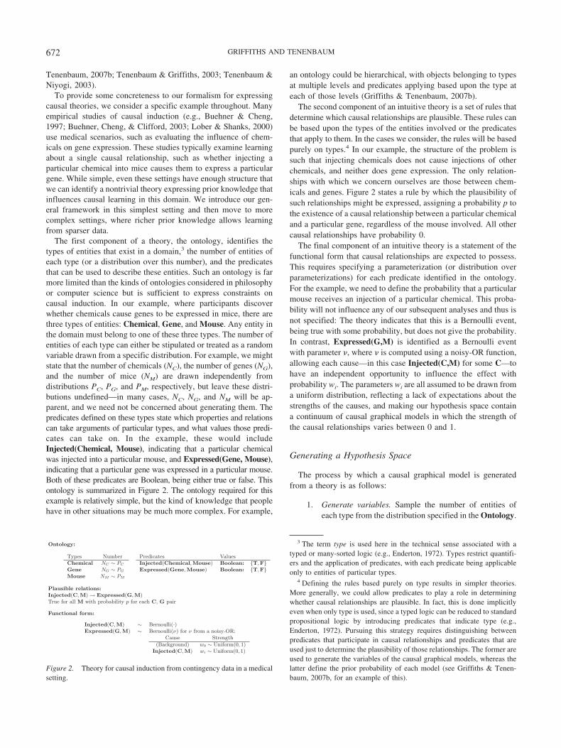
Tenenbaum, 2007b; Tenenbaum & Griffiths, 2003; Tenenbaum &Niyogi, 2003).

To provide some concreteness to our formalism for expressingcausal theories, we consider a specific example throughout. Manyempirical studies of causal induction (e.g., Buehner & Cheng,1997; Buehner, Cheng, & Clifford, 2003; Lober & Shanks, 2000)use medical scenarios, such as evaluating the influence of chem-icals on gene expression. These studies typically examine learningabout a single causal relationship, such as whether injecting aparticular chemical into mice causes them to express a particulargene. While simple, even these settings have enough structure thatwe can identify a nontrivial theory expressing prior knowledge thatinfluences causal learning in this domain. We introduce our gen-eral framework in this simplest setting and then move to morecomplex settings, where richer prior knowledge allows learningfrom sparser data.

The first component of a theory, the ontology, identifies thetypes of entities that exist in a domain,3 the number of entities ofeach type (or a distribution over this number), and the predicatesthat can be used to describe these entities. Such an ontology is farmore limited than the kinds of ontologies considered in philosophyor computer science but is sufficient to express constraints oncausal induction. In our example, where participants discoverwhether chemicals cause genes to be expressed in mice, there arethree types of entities: Chemical, Gene, and Mouse. Any entity inthe domain must belong to one of these three types. The number ofentities of each type can either be stipulated or treated as a randomvariable drawn from a specific distribution. For example, we mightstate that the number of chemicals (NC), the number of genes (NG),and the number of mice (NM) are drawn independently fromdistributions PC, PG, and PM, respectively, but leave these distri-butions undefined—in many cases, NC, NG, and NM will be ap-parent, and we need not be concerned about generating them. Thepredicates defined on these types state which properties and relationscan take arguments of particular types, and what values those predi-cates can take on. In the example, these would includeInjected(Chemical, Mouse), indicating that a particular chemicalwas injected into a particular mouse, and Expressed(Gene, Mouse),indicating that a particular gene was expressed in a particular mouse.Both of these predicates are Boolean, being either true or false. Thisontology is summarized in Figure 2. The ontology required for thisexample is relatively simple, but the kind of knowledge that peoplehave in other situations may be much more complex. For example,

an ontology could be hierarchical, with objects belonging to typesat multiple levels and predicates applying based upon the type ateach of those levels (Griffiths & Tenenbaum, 2007b).

The second component of an intuitive theory is a set of rules thatdetermine which causal relationships are plausible. These rules canbe based upon the types of the entities involved or the predicatesthat apply to them. In the cases we consider, the rules will be basedpurely on types.4 In our example, the structure of the problem issuch that injecting chemicals does not cause injections of otherchemicals, and neither does gene expression. The only relation-ships with which we concern ourselves are those between chem-icals and genes. Figure 2 states a rule by which the plausibility ofsuch relationships might be expressed, assigning a probability p tothe existence of a causal relationship between a particular chemicaland a particular gene, regardless of the mouse involved. All othercausal relationships have probability 0.

The final component of an intuitive theory is a statement of thefunctional form that causal relationships are expected to possess.This requires specifying a parameterization (or distribution overparameterizations) for each predicate identified in the ontology.For the example, we need to define the probability that a particularmouse receives an injection of a particular chemical. This proba-bility will not influence any of our subsequent analyses and thus isnot specified: The theory indicates that this is a Bernoulli event,being true with some probability, but does not give the probability.In contrast, Expressed(G,M) is identified as a Bernoulli eventwith parameter , where is computed using a noisy-OR function,allowing each cause—in this case Injected(C,M) for some C—tohave an independent opportunity to influence the effect withprobability wi. The parameters wi are all assumed to be drawn froma uniform distribution, reflecting a lack of expectations about thestrengths of the causes, and making our hypothesis space containa continuum of causal graphical models in which the strength ofthe causal relationships varies between 0 and 1.

Generating a Hypothesis Space

The process by which a causal graphical model is generatedfrom a theory is as follows:

1. Generate variables. Sample the number of entities ofeach type from the distribution specified in the Ontology.

3 The term type is used here in the technical sense associated with atyped or many-sorted logic (e.g., Enderton, 1972). Types restrict quantifi-ers and the application of predicates, with each predicate being applicableonly to entities of particular types.

4 Defining the rules based purely on type results in simpler theories.More generally, we could allow predicates to play a role in determiningwhether causal relationships are plausible. In fact, this is done implicitlyeven when only type is used, since a typed logic can be reduced to standardpropositional logic by introducing predicates that indicate type (e.g.,Enderton, 1972). Pursuing this strategy requires distinguishing betweenpredicates that participate in causal relationships and predicates that areused just to determine the plausibility of those relationships. The former areused to generate the variables of the causal graphical models, whereas thelatter define the prior probability of each model (see Griffiths & Tenen-baum, 2007b, for an example of this).

Figure 2. Theory for causal induction from contingency data in a medicalsetting.


Generate the complete set of grounded predicates forthese entities. This is the set of variables that form thenodes of the graph.

2. Generate structure. Sample links between nodes usingthe probabilistic procedure stated in the Plausible rela-tions component of the theory.

3. Generate parameterization. For each node, sample aparameterization as specified in the Functional formcomponent of the theory, including the values of therelevant parameters.

This generative process defines a hypothesis space of fully specifiedcausal graphical models, together with a prior probability and, via theparameterization, a likelihood for each model in that space.

We illustrate how this generative process works by using thetheory given in Figure 2. We assume that the number of chemicals,genes, and mice involved in a particular experiment is known, andimplicitly condition on this information. For example, we mighthave a single chemical c, a single gene g, and NM micem1, . . . , mNM

. The set of grounded predicates is constructed bysubstituting all possible entities for the arguments of each predi-cate in the ontology. In our case, this set consists of NM statementsindicating whether Injected(c,mi) holds of mouse mi, and NM

statements indicating whether Expressed(g,mi) holds of mousemi. We then have to consider possible causal structures on these2NM variables. Since the constraints on plausible relations are suchthat if Injected(c,mi) causes Expressed(g,mi) for some mouse mi,then it does so for all mice, we will simply draw an arrow betweentwo variables C and E to indicate that the relationship betweenInjected(c,M) and Expressed(g,M) holds for all mice M. The con-straints on plausible relations imply that the only possible causalrelationship in this graphical model is that from Injected(c,mi) toExpressed(g,mi), and that this relationship holds with probabilityp. The hypothesis space H thus consists of two causal structures:one in which Injected(c,M) causes Expressed(g,M), which hasprior probability p, and one in which Injected(c,M) does not causeExpressed(g,M), which has prior probability 1 – p. These areGraph 1 and Graph 0, respectively, shown at the top of Figure 3.We obtain our full hypothesis space of causal graphical models byaugmenting these structures with parameters w0 and w1 drawnfrom the appropriate prior distribution.

The same procedure can be used to generate a hypothesis spaceof causal graphical models for any number of entities, as illustratedin Figure 3. For example, with two chemicals and two genes, thehypothesis space contains 16 causal graphical models, with theprior probabilities determined by the number of causal relation-ships expressed in the graph. The same causal theory can be usedto define a hypothesis space for five chemicals and 10 genes, or 50chemicals and a thousand genes, simply by applying the sameabstract principles.

Summary

In this section we have outlined some of the key components ofcausal theories and explained how they can be used to generate

hypothesis spaces of causal graphical models. In the followingsections, we present a series of case studies illustrating how thesecomponents vary in different settings and how the constraints thatthey provide are essential to understanding how people learn aboutcausal relationships. These case studies help to illustrate how ourtheory-based approach can provide a unifying account of a broadrange of phenomena related to causal induction: The basic frame-work of statistical inference informed by causal theories remainsconstant, being a domain-general strategy, but the knowledgecontained within the theories varies, allowing us to explaindomain-specific inferences. The influence of the relevant priorknowledge increases as we go through the examples, starting withcausal induction from contingency data where constraints fromprior knowledge are typically weak, but can nonetheless haveinteresting consequences.

Causal Induction From Contingency Data

The aspect of human causal induction that has been studied mostextensively by psychologists is that of inferring a single causal rela-tionship from contingency data. Given information about the fre-quencies with which C and E co-occur, as summarized in Table 1,people are asked to assess the extent to which C causes E. Anumber of mathematical models have been proposed to explainhow people use contingency data to evaluate causal relationships(e.g., Allan, 1980; Anderson, 1990; Anderson & Sheu, 1995;Cheng, 1997; Cheng & Novick, 1990, 1992; Jenkins & Ward,1965; Lopez et al., 1998; Shanks, 1995b). These models tend todownplay the role of prior knowledge, assuming that such knowl-edge serves to provide a set of candidate causes, but contingencydata are used to evaluate those causes.

We provide an account of human causal induction from contin-gency data within our theory-based framework. Most experimentsusing contingency data select candidate causes and effects forwhich causal relationships are plausible. This uniformity of plau-sibility underlies claims about the separability of causal inductionand prior knowledge and means that the aspect of causal theoriesthat determines the plausibility of relationships will not be asrelevant here as in other settings discussed later in the article.However, as our framework emphasizes, prior knowledge is notrestricted to plausibility: It also determines assumptions aboutfunctional form. Our framework thus makes two claims aboutcausal learning from contingency data: that variation in the as-sumed functional form should produce variation in human judg-ments and that causal inferences can be understood as Bayesianinferences about the causal models most likely to have generatedthe observed data.

The plan of this section is as follows. First, we analyze theproblem of causal induction from contingency data using ourtheory-based framework. We then compare the results of thisanalysis with four rational models of human judgments, using thiscomparison to highlight the assumptions behind our analysis thatare critical for predicting human judgments. We go on to test aprediction produced by this analysis, examining whether differenttasks result in different treatment of the statistical problem under-lying causal induction. Finally, we discuss how approaches for-mulating the problem of causal induction in terms of structurelearning and parameter estimation can both be captured within our


framework, consider different strategies that may manifest in thedata, and compare our model to a simple heuristic account.


Buehner and Cheng (1997; see also Buehner, Cheng, & Clifford,2003) conducted an experiment in causal induction from contin-gency data using a medical scenario similar to that outlined in theprevious section: People were asked to rate how strongly theythought the particular rays cause mutation on a scale from 0 (theray does not cause mutation at all) to 100 (the rays cause mutationevery time). Rays and viruses play roles that are directly analogous

to chemicals and genes in our example, and expectations abouttheir causal interactions can be captured using the same causaltheory. The experiment used a design in which 15 sets of contin-gencies expressed all possible combinations of P(e��c�) and �P inincrements of .25. Experiments were conducted with both gener-ative causes, for which C potentially increases the frequency of E,and preventive causes, for which C potentially decreases the fre-quency of E. The results of Buehner and Cheng (1997, Experiment1B), which used generative causes, are shown in Figure 4.

The theory given in Figure 2 can be used to generate a hypoth-esis space of causal models expressing the different kinds of

Hypothesis space for one chemical and one gene

E

C

E

C

E

C C

E E

C C

E E

C C

E

C

E

C

E E

C C

E E

C C

E E

C C

E2

1 2

1 2

1 2

1 2

1 2

1 2

1 2

1

E

C C

E E

C C

E E

C C

E E

C C

E2

1 2

1 2

1 2

1 2

1 2

1 2

1 2

1

E

C C

E E

C C

E E

C C

E E

C C

E2

1 2

1 2

1 2

1 2

1 2

1 2

1 2

1

P(Graph 11) = p (1−p)3

C C

P(Graph 0) = (1−p)4

2

1 2

1 2

1 2

1 2

1 2

1 2

1 2

1

P(Graph 1) = p(1−p)3 P(Graph 2) = p(1−p)

3 P(Graph 3) = p(1−p)3

P(Graph 4) = p(1−p)3 P(Graph 5) = p (1−p) P(Graph 6) = p (1−p) P(Graph 7) = p (1−p)

P(Graph 8) = p (1−p) P(Graph 9) = p (1−p) P(Graph 10) = p (1−p)

P(Graph 12) = p (1−p)3 P(Graph 13) = p (1−p)3 P(Graph 14) = p (1−p)3 4P(Graph 15) = p

E E

P(Graph 0) = 1−p P(Graph 1) = p

Hypothesis space for two chemicals and two genes

222 22 2

2 2 2 2 2 2

Figure 3. Hypothesis spaces generated by the theory shown in Figure 2. The top of the figure shows thehypothesis space for one chemical and one gene, which includes only two causal structures. With two chemicalsand two genes, the hypothesis space includes 16 causal structures, as shown in the lower portion of the figure.In the graphs, C corresponds to Injected(C,M) for Chemical C and E corresponds to Expressed(G,M) for GeneG, both for some mouse M. C1, C2, E1, and E2 should be interpreted similarly. p indicates the probability of acausal relationship existing between a given chemical and gene, as outlined in the theory shown in Figure 2.


structure that might explain the observed data, substituting raysand viruses for chemicals and genes appropriately. For each set ofcontingencies we have a single ray and a single virus, so thehypothesis space H contains the two models Graph 0 and Graph 1shown at the top of Figure 3. The first contribution that the theorymakes to this inference is thus to narrow down the hypothesisspace of possible causal structures to just two, ruling out otherstructures in which viruses cause the application of rays or hiddencommon causes exist. According to the theory, these two modelsshould use the noisy-OR parameterization, with each cause inde-pendently having the chance to influence the effect. In fact, each ofthese graphical structures corresponds to a continuum of causalmodels, each with different values of w0 and w1, with the priorbeing uniform over these values.

We can explore a variety of ways of answering the question thatparticipants were asked in this experiment. While the question isnominally about the strength of the causal relationship, it is rela-tively ambiguous and previous work has suggested that people canstill produce responses consistent with making an inference aboutcausal structure when faced with such a question (Griffiths &Tenenbaum, 2005). For consistency with the other models weconsider in this article, we focus for now on modeling these resultsas the consequence of a structural inference, although we return tothe issue of the roles of structure and strength in causal inductionlater in the section.

Under this hypothesis space, the probability that a causal rela-tionship exists is the probability that Graph 1 was responsible forgenerating the data, D, being the frequencies with which cause andeffect co-occurred. We thus want to compute

P�Graph 1�D�

�P�D�Graph 1�P�Graph 1�

P�D�Graph 1�P�Graph 1� � P�D�Graph 0�P�Graph 0�,

(5)

which is simply Bayes’ rule, applied to the two hypotheses Graph0 and Graph 1. The theory defines P(Graph 1) and P(Graph 0) viathe parameter p, which we set to .5. Computing P(D�Graph 1) andP(D�Graph 0) requires integrating over the values of the parame-ters of these models. The details of computing such integrals arediscussed in Griffiths and Tenenbaum (2005), where essentiallythe same model is used to account for a range of phenomena incausal induction from contingency data.5

Figure 4 displays P(Graph 1�D) for different sets of contingen-cies D, under this noisy-OR model. There is a remarkably closecorrespondence between the predictions of the model and people’sjudgments. The rank-order correlation between the probabilities

and human responses is � .971. The model also seems to captureall of the important trends in the data, including the curious trendshown by the leftmost five stimuli in the figure: People’s judg-ments increase as P(e��c�) increases, despite the fact that there isno difference in the probability of the effect in the presence andabsence of the cause. This phenomenon is known as the frequencyillusion or the outcome density effect (Allan & Jenkins, 1983;Shanks, Lopez, Darby, & Dickinson, 1996), and, as we shall seeshortly, presents a challenge for other models of causal induction.

Alternative Accounts

We can gain insight into the critical features of this account ofcausal induction from contingency data by comparing its predic-tions to those of other models. Our theory-based account assumesthat people approach causal induction as a decision between dif-ferent causal structures and that their intuitive theory involves afunctional form equivalent to the noisy-OR. We consider twoclasses of models that can be used to evaluate these assumptions.One class treats causal induction as a problem of estimating thestrength of a causal relationship, rather than inferring the under-lying causal structure. The two models in this class are the rationalmodels of causal induction from contingency data introducedabove, causal power (Cheng, 1997), and �P (Jenkins & Ward,1965). The other class of models focuses on learning causalstructure but does not make strong assumptions about the func-tional form of the underlying causal relationship. The two modelsin this class correspond to the two approaches to structure learningthat have been pursued by computer scientists and statisticians: �2,the frequentist test of statistical dependence used in constraint-based algorithms, and Bayesian inference comparing causal mod-els with a generic parameterization. Since these models have notbeen fully introduced, the next two paragraphs provide the relevantmathematical details.

The first step of constraint-based algorithms for learning causalstructure is to evaluate the dependencies among a set of variables.This is typically done using the standard frequentist analysis ofcontingency tables, Pearson’s (1904/1948) �2 test for indepen-dence. The use of the �2 test as a model of human causal judgmentwas suggested in the psychological literature (e.g., Allan, 1980)but was rejected on the grounds that it neglects the kind ofasymmetry that is inherent in causal relationships, providing in-formation solely about the existence of statistical dependencybetween the two variables (Allan, 1980; Lopez et al., 1998;Shanks, 1995b). �2 also makes no commitment about the func-tional form of the relationship between cause and effect: It simplydetects any kind of statistical dependency between C and E.

5 The basic model we explore in this section expresses the assump-tions behind the causal support model introduced by Griffiths andTenenbaum (2005) in our formal framework. Causal support was com-pared to human ratings using a power function of the log-likelihood ratio,

logP�D�Graph 1�

P�D�Graph 0�, rather than the posterior probability P(Graph 1�D). We

choose to use the posterior probability here for simplicity, and for consis-tency with the other examples discussed in the article. The posteriorprobability can also be obtained via a logistic transformation of the log-likelihood ratio, so the two models are related by a monotonic transfor-mation.

Table 1Contingency Table Representation Used in Causal Induction

Cause

Effect

Present (e�) Absent (e�)

Present (c�) N(e�c�) N(e�c�)Absent (c�) N(e�c�) N(e�c�)

Note. N(�) denotes the frequency of a particular event.


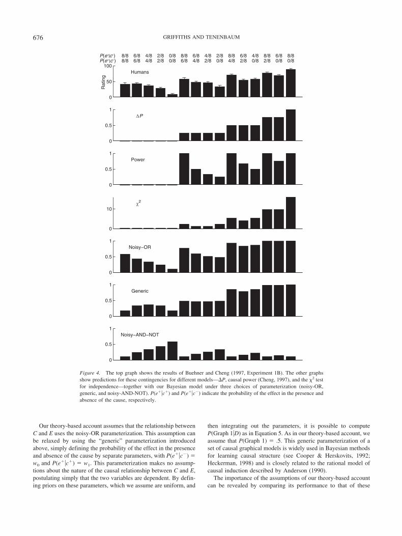
Our theory-based account assumes that the relationship betweenC and E uses the noisy-OR parameterization. This assumption canbe relaxed by using the “generic” parameterization introducedabove, simply defining the probability of the effect in the presenceand absence of the cause by separate parameters, with P(e��c�) �w0 and P(e��c�) � w1. This parameterization makes no assump-tions about the nature of the causal relationship between C and E,postulating simply that the two variables are dependent. By defin-ing priors on these parameters, which we assume are uniform, and

then integrating out the parameters, it is possible to computeP(Graph 1�D) as in Equation 5. As in our theory-based account, weassume that P(Graph 1) � .5. This generic parameterization of aset of causal graphical models is widely used in Bayesian methodsfor learning causal structure (see Cooper & Herskovits, 1992;Heckerman, 1998) and is closely related to the rational model ofcausal induction described by Anderson (1990).

The importance of the assumptions of our theory-based accountcan be revealed by comparing its performance to that of these

0

50

100

8/88/8

6/86/8

4/84/8

2/82/8

0/80/8

8/86/8

6/84/8

4/82/8

2/80/8

8/84/8

6/82/8

4/80/8

8/82/8

6/80/8

8/80/8

P(e+ c+)P(e+ c−)

Humans

0

0.5

1∆ P

0

0.5

1Power

0

10χ2

0

0.5

1

Rat

ing

Noisy−OR

0

0.5

1Generic

0

0.5

1Noisy−AND−NOT

||

Figure 4. The top graph shows the results of Buehner and Cheng (1997, Experiment 1B). The other graphsshow predictions for these contingencies for different models—�P, causal power (Cheng, 1997), and the �2 testfor independence—together with our Bayesian model under three choices of parameterization (noisy-OR,generic, and noisy-AND-NOT). P(e��c�) and P(e��c�) indicate the probability of the effect in the presence andabsence of the cause, respectively.


different models. Causal power uses the functional form identifiedin Figure 2, but it models judgments as strength estimation. Com-paring our model with causal power thus reveals the role ofcharacterizing human inferences as an inference about causalstructure rather than an inference about causal strength. �2 and thegeneric Bayesian approach are both concerned with causal struc-ture but make weak assumptions about functional form. Compar-ison with these models reveals the importance of the assumptionsabout functional form embodied in the causal theory that underliesour model.

The predictions of all of these models are shown in Figure 4, andthe rank-order correlations between models and human judgmentsare summarized in Table 2. None of the models had any freeparameters, and the predictions were not transformed to fit the databecause the rank-order correlation is unaffected by monotonictransformations. Our theory-based model matched or exceeded theperformance of the other models. Both �P and causal poweraccounted for some of the trends in the data—for example, �Pcaptures the increase in judgments as P(e��c�) – P(e��c�) in-creases, and causal power generally captures the increase in judg-ments as P(e��c�) increases—but these trends are essentiallyorthogonal, and consequently neither model provides a completeaccount of the data. The theory-based noisy-OR model predictsboth of these trends and is the only model that accurately predictshuman judgments for the five stimuli on the left of the figure—those for which �P � 0. People’s assessment of the extent towhich it seems that C causes E decreases as P(e��c�) decreases.The fact that none of the other models predicts these judgmentsreveals that these predictions are the direct consequence of com-bining a particular functional form (the noisy-OR) with Bayesianstructure learning. We now examine why the theory-based modelmakes this prediction.

The Importance of Functional Form

The fact that human judgments decrease as P(e��c�) decreaseswhen �P � 0 seems counterintuitive: There is no difference in the

probability of the effect in the presence or absence of the cause forany of these stimuli, so why should people change their belief thata causal relationship exists? In our theory-based account, theexplanation for these predictions is not that there is decreasingevidence for a causal relationship as P(e��c�) decreases, but ratherthat there is no evidence for or against a causal relationship whenP(e��c�) � 1, and increasing evidence against a causal relation-ship as P(e��c�) decreases. This account depends on the assumptionthat the causal relationship—if it exists—is generative (increasing theprobability of the effect, rather than preventing it). This assumption isa key part of the theory shown in Figure 2 and manifests in the use ofthe noisy-OR parameterization. At one extreme, when {P(e��c�),P(e��c�)} � {8/8, 8/8}, all viruses mutated irrespective of ray expo-sure, and it is clear that there is no evidence for a causal relationship.But there can also be no evidence against a (generative) causalrelationship, because of a complete “ceiling” effect: It is impossiblefor the cause to increase the probability of E occurring above itsbaseline value when P(e��c�) � 1. This uncertainty in causaljudgment when P(e��c�) � 1 and �P � 0 is predicted by both ourmodel, in which P(Graph 1�D) is close to .5, and also (as Cheng,1997, pointed out) by causal power, which is undefined for thesecontingencies.

Only the noisy-OR model, however, predicts the gradient ofjudgments as P(e��c�) decreases. P(Graph 1�D) decreases as theceiling effect weakens and the observation that �P � 0 providesincreasing evidence against a generative causal relationship. At theother extreme, when P(e��c�) � 0/8, no unexposed viruses mu-tated, and there are eight opportunities for a causal relationship tomanifest itself in the exposed viruses if such a relationship in factexists. The fact that the effect does not appear in any exposedviruses, P(e��c�) � 0/8, suggests that the ray does not cause virusmutation. The intermediate cases provide intermediate evidenceagainst a causal relationship. The contingencies {2/8, 2/8} offer sixchances for the cause to have an effect, and the fact that it neverdoes so is slightly weaker evidence against a relationship than inthe {0/8, 0/8} case, but more compelling than for {6/8, 6/8}, where

Table 2Rank-Order Correlations for Different Models of Causal Induction

Model

Buehner and Cheng (1997) Functional form experiment

Generative Preventive Generative Difference Preventive

Bayesian modelsNoisy-OR .961 �.814 .971 .850 �.721Generic .876 .760 .957 .975 .930Noisy-AND-NOT �.868 .893 �.732 �.336 .971

�PPositive .883 �.769 .968 �.946Absolute value .883 .769 .968 .968 .946Negative �.883 .769 �.968 .946

PowerGenerative .942 �.531 .949 �.800Preventive �.698 .884 �.858 .971

�2 .880 .761 .966 .958 .940

Note. Boldface indicates the highest correlation in each column. Many of the correlations listed in the table represent combinations of models and tasksthat have not been advocated in the literature, such as using the preventive version of causal power to model inferences about generative causes. We includethese correlations for completeness, and because they provide a clear verification of the need for models assuming different functional forms for differenttasks.


the cause has only two chances to manifest itself and the obser-vation that �P � 0 could easily be a coincidence. This gradient ofuncertainty shapes the Bayesian structural inference that underliesour model, but it does not affect the maximum-likelihood param-eter estimates underlying causal power or �P.

This explanation depends upon two aspects of our theory-basedaccount: the general assumption that causal induction is a statisti-cal inference comparing causal structures and the specific assump-tion that the appropriate functional form is the noisy-OR. Theimportance of these assumptions is supported by the failure ofcausal power, an estimate of the strength of a causal relationshipunder the noisy-OR, and the generic Bayesian structure-learningmodel. One prediction of this account is that people should altertheir judgments in circumstances where a different functional formis appropriate. An opportunity to test this prediction comes frompreventive causes. Since the noisy-OR only allows causes toincrease the probability of their effects, a different parameteriza-tion is required to capture the properties of causes that decrease theprobability of their effects. Buehner and Cheng (1997, Experiment1A) used a design similar to that already described for generativecauses to assess people’s judgments about preventive causes. Theresults of this experiment are shown in Figure 5. From the figure,it can be seen that the trend at �P � 0 is reversed for preventivecauses: A decrease in P(e��c�) results in an increase in people’sjudgments.

Modeling these data requires making an assumption about thefunctional form of preventive causes. A simple theory of this kindwould have the same content as the theory for generative causesshown in Figure 2, except for the assumptions about functionalform, replacing the noisy-OR with the noisy-AND-NOT parame-terization (Cheng, 1997; Novick & Cheng, 2004; Pearl, 1988).This parameterization follows from a set of assumptions similarto those made in the noisy-OR. In the case of Graph 1, theseassumptions are that E occurs in the absence of C with probabilityw0, and C independently prevents E from occurring with proba-bility w1. The resulting parameterization generalizes the logicalstatement that E will occur if the background factors are presentand not C, allowing the influence of these factors to be probabi-listic. The conditional probability can be written as

P�e��c; w0, w1� � w0�1 � w1�c, (6)

which gives w0 for the probability of E in the absence of C andw0(1 – w1) when C is present. As with the noisy-OR, both w0 andw1 are constrained to lie in the range [0, 1], and the function canbe generalized to accommodate the influence of multiple parents.

Under a theory using the noisy-AND-NOT, the posterior prob-abilities of different causal structures can still be evaluated viaEquation 5, but the different parameterization results in differentprobabilities for P(D�Graph 1) and P(D�Graph 0). First, we notethat comparing structures with the noisy-AND-NOT parameteriza-tion provides a poor account of human judgments for generativecauses, as shown in Figure 4 and Table 2. This model is actuallystrongly anticorrelated with human judgments for generativecauses. However, the noisy-AND-NOT model gives a good ac-count of human judgments for preventive causes, with � .893.The predictions of this model are shown in Figure 5.

The alternative models discussed above can also be applied tothis preventive setting. Rather than using �P to predict judgmentsabout preventive causes, we use –�P. Cheng (1997) defined causal

power for preventive causes, following from a set of assumptionssimilar to those made for generative causes. The causal power fora preventive cause is

power ��P

P�e��c��. (7)

The effect of P(e��c�) on causal power is the reverse of that forgenerative causes, with �P having a greater influence whenP(e��c�) is small. Tenenbaum and Griffiths (2001; Griffiths &Tenenbaum, 2005) showed that this form of causal power is amaximum-likelihood estimate of the w1 parameter for the noisy-AND-NOT. �2 and Bayesian structure learning with the genericparameterization are unaffected by the valence of a causal rela-tionship and can be applied just as in the generative case.

The predictions of these models are shown in Figure 5, and theircorrelations with human judgments are given in Table 2. Bayesianstructure learning with the noisy-AND-NOT outperformed allother models and gave a better account of human judgments thanBayesian structure learning with either the noisy-OR or the genericparameterization. This included accurately predicting the trendshown by the stimuli for which �P � 0, which goes in the oppositedirection from that for generative causes, but has the same statis-tical explanation—since causes decrease the probability of effectsin the preventive setting, {8/8, 8/8} gives the most opportunities todiscover that the cause does not influence the effect.

Inferences about generative causes are best captured using anoisy-OR parameterization, and inferences about preventivecauses are best captured by the noisy-AND-NOT. This suggeststhat people make different assumptions about the functional formof generative and preventive causes and is consistent with theanalysis of generative and preventive causal relationships given byCheng (1997) and Novick and Cheng (2004). A further questionraised by these results is whether there are any circumstancesunder which people’s judgments will be best captured by thegeneric parameterization. The generic parameterization makes noassumptions about the nature of the relationship between cause andeffect. Bayesian structure learning with this parameterizationamounts to assessing whether there is any difference in the prob-ability with which the effect occurs in the presence and absence ofthe cause. Consequently, we would expect that explicitly askingpeople to assess whether there is a difference in the probabilitywith which the effect occurs under two different conditions willproduce responses consistent with the generic parameterization.

To test this hypothesis, we ran an experiment in which peoplewere asked to evaluate a set of contingencies as either evidence fora generative causal relationship between injecting a chemical intoa mouse and a gene being expressed, evidence for a preventivecausal relationship between injecting a chemical and a mousecatching a virus, or evidence for a difference in the probability ofgene expression between two species of mice. The generativecondition used the contingencies from Buehner and Cheng (1997,Experiment 1B), as given in Figure 4; the preventive conditionused the contingencies from Buehner and Cheng (1997, Experi-ment 1A). These contingencies differ only in whether P(e��c�) isgreater than P(e��c�) or vice versa. The difference condition usedthe same contingencies, randomizing whether the probability ofthe effect was higher for the first species or the second. In eachcase, these stimuli were presented on a one-page survey, which


outlined the medical cover story and then asked people to evaluatethe evidence provided by the contingencies, stating that each set ofcontingencies indicated the results of a laboratory study (the fullscenarios appear in Appendix A). In the generative condition,participants were given the following instructions:

For each study, write down a number between 0 and 100 representingthe degree to which the chemical causes the gene to be expressed. Arating of 0 indicates that the chemical DOES NOT CAUSE the geneto be expressed at all, and a rating of 100 indicates that the chemical

DOES CAUSE the gene to be expressed every time. Use intermediateratings to indicate degrees of causation between these extremes.

In the preventive condition, the instructions read as follows:

For each study, write down a number between 0 and 100 representingthe degree to which the chemical prevents a virus being caught. Arating of 0 indicates that the chemical DOES NOT PREVENT thevirus at all, and a rating of 100 indicates that the chemical DOESPREVENT the virus every time. Use intermediate ratings to indicatedegrees of prevention between these extremes.

0

50

100

8/88/8

6/86/8

4/84/8

2/82/8

0/80/8

6/88/8

4/86/8

2/84/8

0/82/8

4/88/8

2/86/8

0/84/8

2/88/8

0/86/8

0/88/8

P(e+ c+)P(e+ c−)

Humans

0

0.5

1∆ P

0

0.5

1Power

0

10χ2

0

0.5

1

Rat

ing

Noisy−OR

0

0.5

1Generic

0

0.5

1Noisy−AND−NOT

||

Figure 5. The top graph shows the results of Buehner and Cheng (1997, Experiment 1A). The other graphsshow predictions for these contingencies for different models—�P, causal power (Cheng, 1997), and the �2 testfor independence—together with our Bayesian model under three choices of parameterization (noisy-OR,generic, and noisy-AND-NOT). P(e��c�) and P(e��c�) indicate the probability of the effect in the presence andabsence of the cause, respectively.


Finally, the difference condition gave these instructions:

For each study, write down a number between 0 and 100 representinghow likely you think it is that the two species differ in their probabilityof expressing that gene. A rating of 0 indicates that the two speciesDEFINITELY have THE SAME probability of expressing the gene,while a rating of 100 indicates that the two species DEFINITELYhave DIFFERENT probabilities of expressing the gene. Use interme-diate ratings to indicate degrees of likelihood between these extremes.

Participants completed the survey as part of a booklet of unrelatedsurveys. There were 73 participants in the generative condition, 47in the difference condition, and 67 in the preventive condition.

People’s judgments in the generative and preventive conditionsreplicated the results of Buehner and Cheng (1997), having a linearcorrelation of r � .993 and r � .989 with Experiments 1B and 1A,respectively (we used linear rather than rank-order correlationshere since there was no need to take into account possible nonlin-ear transformations). The correlations between Bayesian structure-learning models and these judgments are shown in Table 2. Alsoincluded in the table are the predictions of �P, causal power, and�2 (the absolute value of �P was used for the difference condition,but there was no appropriate analogue of causal power). As pre-dicted, the noisy-OR model gave the best account of responses inthe generative condition, the generic model did best in the differ-ence condition, and the noisy-AND-NOT did best in the preventivecondition. Human judgments for the five stimuli for which �P �0 are shown in Figure 6. �P, causal power, and �2 all predict thatthere should be no variation in responses across these stimuli.Contrary to these predictions, the effect of P(e��c�) on judgmentswas statistically significant in both the generative, F(4, 288) �5.32, MSE � 216.92, p � .001, and preventive conditions, F(4,264) � 2.63, MSE � 313.25, p � .05, and approached significancein the difference condition, F(4, 184) � 2.40, MSE � 345.74, p �.051. There was also a statistically significant interaction betweenP(e��c�) and condition, F(8, 736) � 3.68, MSE � 283.68, p �.001. As can be seen from the figure, this variation was exactly as

should be expected if people are performing Bayesian structurelearning with the appropriate parameterization.

Structure, Strength, and Strategies

The models we have presented in this section are based on theassumption that people are making a judgment about whether ornot a causal relationship exists, rather than estimating its strength.As we noted when we first defined our framework, this is not anecessary assumption: By taking our hypotheses to include both acausal structure and the values of the appropriate parameters, it isalso possible to define models that correspond to Bayesian strengthestimation of the kind endorsed by Lu et al. (2007, 2008). Whetherstructure or strength is relevant will be determined by the demandsof the task. For example, Buehner et al. (2003) have shown thatpeople tend to produce judgments that are more consistent withcausal power when they are asked a counterfactual question, suchas “What is the probability that a mouse not expressing the genebefore being injected will express it after being injected with thechemical?” As pointed out by Griffiths and Tenenbaum (2005, pp.374–375) this finding is consistent with the analysis we havepresented in this section, since the rational answer to this questionshould be an estimate of w1. The Bayesian treatment of strengthestimation presented by Lu et al. (2007, 2008) provides a way toincorporate the effects of prior knowledge into these strengthestimates.

Even in cases where people’s judgments seem to be bettercharacterized in terms of structure learning, there is room forvariation in the assumptions we make about the knowledge thatinforms these judgments. The model we have presented in thissection makes the simplest possible assumption about the prior onthe strength parameters w0 and w1, considering each value of theseparameters to be equally likely. However, this assumption has aneffect on the model’s predictions both about the probability that acausal relationship exists and about the strength of that relation-ship. Lu et al. (2006, 2007, 2008) have shown that adopting a more

0

20

40

8/88/8

6/86/8

4/84/8

2/82/8

0/80/8

P(e+ c+)

Generative

Rat

ing

8/88/8

6/86/8

4/84/8

2/82/8

0/80/8P(e+ c-)

Generative

8/88/8

6/86/8

4/84/8

2/82/8

0/80/8

Generative

0

20

40

8/88/8

6/86/8

4/84/8

2/82/8

0/80/8

Difference

8/88/8

6/86/8

4/84/8

2/82/8

0/80/8

Difference

8/88/8

6/86/8

4/84/8

2/82/8

0/80/8

Difference

0

20

40

8/88/8

6/86/8

4/84/8

2/82/8

0/80/8

Preventive

8/88/8

6/86/8

4/84/8

2/82/8

0/80/8

Preventive

8/88/8

6/86/8

4/84/8

2/82/8

0/80/8

Preventive

0

0.2

0.4

0.6

0.8

Noisy−OR

P(G

raph

1 D

)

0

0.2

0.4

0.6

0.8

Generic

0

0.2

0.4

0.6

0.8

Noisy−AND−NOT

||

|

Figure 6. Effect of assumptions about functional form on causal induction. The top row shows people’sjudgments for a set of stimuli for which �P � 0, under three different kinds of instructions, as described in thetext. The bottom row shows the predictions of our theory-based account under three different assumptions aboutthe functional form of a causal relationship. There appears to be a direct correspondence between taskinstructions and assumed functional form. P(e��c�) and P(e��c�) indicate the probability of the effect in thepresence and absence of the cause, respectively.


informative prior on w0 and w1, in which causes are assumed to bestrong when they exist and the values of w0 and w1 are inverselycorrelated, can improve the performance of this model for bothstructure learning and strength estimation. This modification canbe incorporated into our framework through a small change in thepart of the theory that specifies the functional form, replacing theuniform prior with this more informative version.

Whether people approach a task as structure learning or strengthestimation will depend on their interpretation of the task and thestrategies that they adopt. More generally, the richer characteriza-tion of the knowledge that people can bring to bear on a causalinduction task provided by our framework opens up some inter-esting opportunities in understanding individual differences. Forexample, Buehner et al. (2003) noted that there appeared to besignificant individual differences in the judgments that peopleproduced in the experiment that we used to introduce our model.They performed a cluster analysis and found two clusters, one ofwhich correlated well with causal power ( � .902) and the otherwith �P ( � .968). The mean ratings for the two clusters areshown in Figure 7. On the basis of these findings, other researchershave considered the possibility of modeling human judgments as alinear combination of �P and causal power (Perales & Shanks,2007). However, our framework suggests another possibility: thatthese individual differences were not the consequence of differentstrategies, but different assumptions about the nature of causalrelationships. Figure 7 shows that these two clusters of subjectsactually seem to correspond more closely with the predictions ofthe Bayesian model using two different parameterizations: anoisy-OR for the first cluster and a generic parameterization forthe second cluster. Rank-order correlation coefficients of � .946and � .980, respectively, strongly support these accounts. Itappears that everyone in this experiment is judging the evidentialsupport for a causal relationship, but one group appears to bethinking of that causal relationship in terms of a generative mech-anism whereas the other makes a weaker assumption that the causeis just a “difference maker” in the probability of the effect. Ex-ploring the extent to which individual differences can be explainedas a consequence of variation in the construal of the assumptionsthat people make about causal induction tasks is an interestingdirection for future work.

Comparing to Other Models

Causal induction from contingency data has been the target ofan unusually large number of computational models, and ourdiscussion so far has focused on a comparison with just fourmodels. These models were selected to highlight the contributionsof the key components of our framework as clearly and briefly aspossible, since the focus of this article is on capturing the effectsof prior knowledge rather than developing the best model of causalinduction from contingency data. However, two recent meta-analyses that compared the predictions of several models to humanjudgments across several experiments provide a way to get a sensefor how well the model we have used as the basis for our analysisperforms in comparison to other models of causal induction.

Hattori and Oaksford (2007) compared 41 models against hu-man judgments from 143 sets of contingencies derived from fivesets of experiments including their own, including only sets ofcontingencies consistent with generative causes. Models were as-

sessed by computing the linear correlation within each experiment(or set of experiments in one case), and then aggregating thesecorrelations to compute an overall average. Our Bayesian approachgave the fifth best performance of the 34 models without freeparameters, despite the use of an arbitrary monotonic transforma-tion of the model predictions in order to compute the correlation.Two of the models that gave higher correlations were heuristicaccounts based on combining the frequencies that appear in thecells of the contingency table, using weights established throughprevious experiments. The other two models were variations on thescheme that Hattori and Oaksford (2007) were advocating in theirarticle. Consistent with the results presented in this section, ourBayesian model performed better than both causal power and �P.

Perales and Shanks (2007) performed a similar meta-analysis,including 114 sets of contingencies derived from eight sets ofexperiments, with some overlap with those considered by Hattoriand Oaksford (2007). Unlike Hattori and Oaksford, the experi-ments testing these sets of contingencies used instructions thatasked people to evaluate generative causes, preventive causes, orleft the valence of the cause unspecified. The models consideredincluded causal power, �P, a weighted mixture of causal powerand �P, our Bayesian account, a heuristic based on a weightedcombination of cell frequencies, and two associative learningmodels. Models were assessed by computing a single linear cor-relation with human judgments across the full set of contingencies.In their analysis, our Bayesian approach gave the worst perfor-mance of all models being considered, with an overall correlationof r � .81, worse than �P (r � .89), causal power (r � .92), andthe heuristic model (r � .94).

The criteria by which Perales and Shanks (2007) chose datasetsfor inclusion in their analysis were not particularly favorable torational models, since they emphasized online learning, mixedpreventive and generative causes, and allowed response scalesranging from �100 (indicating a strong preventive relationship) to100 (indicating a strong generative relationship). As they note intheir article, their application of our Bayesian model did notresolve the problems created by mixing types of causes (whichresult in different predictions from the model) or provide a well-motivated solution to the problem of mapping to a scale from�100 to 100. One way to solve both of these problems is to definea hypothesis space that includes variation in functional form. Forexample, with just one potential cause C and effect E we candefine a hypothesis space containing three structural hypotheses:Graph 0, in which no causal relationship exists; Graph �, in whicha generative (noisy-OR) relationship exists; and Graph �, in whicha preventive (noisy-AND-NOT) relationship exists. All threestructural hypotheses are also associated with a continuum ofvalues for w0 and w1, defining a complete hypothesis space of fullyspecified graphical models. We can then use Bayes’ rule to com-pute the posterior distribution over these hypotheses and take thepredicted response to be �100P(Graph –�D) � 100P(Graph ��D),where we obtain the probabilities for each graph by integratingover the values of w0 and w1 as before. This response rule reducesto the posterior probability that a causal relationship exists (ex-pressed as a percentile) when the valence of the causal relationshipis known, and it is thus consistent with the other Bayesianstructure-learning models presented in this section.

We applied this revised model to the sets of contingenciesconsidered by Perales and Shanks (2007). When the valence of the


cause was unambiguous, established through experimental instruc-tions and the use of a rating scale that allowed only a single sign,the Bayesian structure-learning model with the appropriate func-tional form was used. When the valence was ambiguous, the modelallowing both functional forms was used. The prior was taken to beuniform over all hypotheses in each case. Resolving the issues ofdetermining the appropriate functional form and response mapping

resulted in a large improvement in fit, with the model producingr � .93. Thus, when the consequences of mixing generative andpreventive causes are taken into account, the model produces acorrelation that is higher than that of both causal power and �P,and very close to that of the best-performing heuristic model. Luet al. (2008) have shown that a similarly high correlation can beobtained by using a Bayesian strength estimation model using a

0

50

100

8/88/8

6/86/8

4/84/8

2/82/8

0/80/8

8/86/8

6/84/8

4/82/8

2/80/8

8/84/8

6/82/8

4/80/8

8/82/8

6/80/8

8/80/8

P(e+ c+)P(e+ c−)

Cluster 1

(a)

Rat

ing

0

50

100

Power

0

50

100

Noisy−OR

0

50

100

8/88/8

6/86/8

4/84/8

2/82/8

0/80/8

8/86/8

6/84/8

4/82/8

2/80/8

8/84/8

6/82/8

4/80/8

8/82/8

6/80/8

8/80/8

P(e+ c+)P(e+ c−)

Cluster 2

(b)

Rat

ing

0

50

100

∆ P

0

50

100

Generic

||

||

Figure 7. Mean ratings for two clusters of participants in Buehner and Cheng (1997, Experiment 1B), basedon the analysis performed by Buehner et al. (2003). (a) The first cluster was interpreted as reflecting causalpower, but also seems consistent with Bayesian structure learning using a noisy-OR parameterization. (b) Thesecond cluster was interpreted as corresponding to �P, but also seems consistent with Bayesian structurelearning using a generic parameterization. P(e��c�) and P(e��c�) indicate the probability of the effect in thepresence and absence of the cause, respectively.


uniform prior, and that an even higher correlation results from useof an informative prior. Given that the fit of the heuristic modelalso depends on setting several unmotivated free numerical param-eters, we take these results on balance to favor our Bayesianapproach to causal learning, contrary to the conclusions of Peralesand Shanks.

Summary

Learning a single causal relationship from contingency data isarguably the most basic form of causal learning and is certainlythat which has inspired the most psychological research. Theresults discussed above suggest that causal theories play a subtlebut important role in guiding causal induction from contingencydata. Models developed using our theory-based approach outper-form leading rational models—�P and causal power—as well asmodels based upon standard algorithms for causal learning devel-oped in computer science and statistics. The success of thesemodels can be traced to two factors: the use of a causal theory thatnarrows down the hypothesis space and postulates the correctfunctional form, and the formulation of causal induction as aBayesian inference about the causal model most likely to havegenerated the observed data. Varying the context of causal learningalters the functional form that people assume and the way that theyconstrue the statistical problem, resulting in variations in behaviorthat can be explained within this framework.

Although we have focused on the effects of just three differ-ent parameterizations in the context of learning about a singlecausal relationship, the particular parameterization that learnersshould use will depend on the context in which learning takesplace. Different settings will result in different expectationsabout the nature of causal relationships. Consequently, there aremany directions in which this analysis could be extended. Asimple next step would be to explore the contexts in whichfunctional forms corresponding to the kinds of causal schemasthat Kelley (1973) identified are used, and how people mightlearn that such schemas are appropriate. Understanding how togeneralize the approach we have taken here to predict otherbehavioral data, such as acquisition curves (e.g., Shanks, 1987),is also important, and will require working out how to translatethis kind of rational analysis into predictions about the processof learning (see Danks et al., 2003, for some initial steps in thisdirection). More ambitiously, it will be important to take thisapproach beyond the case of a single causal relationship inorder to make predictions about causal induction in contextswhere causes interact (e.g., Dickinson, Shanks, & Evenden,1984; Novick & Cheng, 2004; Price & Yates, 1993). Now weturn to a different setting, in which more complex causalstructures are considered but theories provide even strongerconstraints on causal models, making it possible to infer causalrelationships from far fewer observations.

Inferences From Small Samples

Although causal learning from contingency data typically in-volves presenting a large number of observations of cause andeffect, much of human causal learning proceeds on far smallersamples. For example, flipping a switch once and observing a lightcome on is normally sufficient to convince us of the existence of

a causal relationship. The human ability to infer causal relationshipsfrom small samples is at odds with the idea that people infer causalrelationships purely from contingencies, and for standard algorithmsfor causal learning. For Hume (1748/1977, p. 52), causal inductionrequired “many uniform instances.” Similarly, the statistical tests thatscientists use to evaluate causal claims, and which are at the heart ofmany generic algorithms for learning causal graphical models (e.g.,Pearl, 2000; Spirtes et al., 1993), require large samples to achievesignificance. One of the key challenges for a computational account ofhuman causal inferences is thus explaining how it is possible forpeople to learn so much from so little.

Explaining rapid causal learning might not seem problematic foradvocates of the idea that human causal induction can be explainedin terms of associative learning (e.g., Shanks, 1995b). Models ofassociative learning, such as the Rescorla-Wagner model (Rescorla& Wagner, 1972), typically incorporate a parameter that plays therole of a learning rate, determining how much people modify theirestimates of the strength of a causal relationship on the basis oftheir experiences in a single trial of learning. A high learning rateresults in rapid learning, with only a few trials being sufficient toproduce a large change in the estimate of the strength of a causalrelationship. Human inferences from small samples might thus beaccounted for by saying that people have a high learning rate.However, this kind of account seems unsatisfying. In explaininghow it is possible for people to learn so much from so little, wewould also hope to explain why this seems to take place in somesituations but not others. Flipping a switch once might seem toprovide definitive evidence about the existence of a causal rela-tionship, but running an experiment in which a single participantproduces a single response that is consistent with our predictions isunlikely to convince us that we have discovered a new causalrelationship. Saying that we have a high learning rate for lightswitches and a low learning rate for psychology experimentsseems like a redescription of the data. A more satisfying explana-tion would be a systematic account that predicts under whatcircumstances we should expect causal induction to be rapid andunder what circumstances we might be willing to believe in acausal relationship only after collecting many observations.

An intuitive answer to the question of how people learn so muchfrom so little is that their inferences are informed by prior knowl-edge, and that this knowledge is itself acquired through experi-ence. This is essentially the answer that we will provide, arguingthat causal induction from small samples can be explained as theresult of a combination of strong constraints from relatively so-phisticated causal theories with statistical inference. The challengehere is in showing that this prior knowledge interacts with the ob-served data in a nontrivial way. We show that the kind of knowledgethat is relevant to producing correct causal inferences from smallsamples goes beyond forming generalizations based on more abstractcategories of causes (Lien & Cheng, 2000) or the a priori plausibilityof causal relationships (Alloy & Tabachnik, 1984), although these areobviously both important ways in which prior knowledge can affectpeople’s inferences. In particular, we argue that assumptions aboutfunctional form are one of the key factors in enabling causal inductionfrom small samples. Thus, we can draw strong conclusions fromflipping a switch but not from the response of a single experimentalparticipant because we expect the former causal relationship to be


deterministic but the latter to be probabilistic.6 This argument boilsdown to learners having expectations about the variability associ-ated with causal relationships, which will influence the amount ofdata that they need to see in a way that generalizes to otherinductive problems as well (for a similar argument, see Holland,Holyoak, Nisbett, & Thagard, 1986).

We support our analysis by examining the inferences that chil-dren and adults make in a context where they have strong priorknowledge: reasoning about the behavior of a machine for detect-ing the hidden properties of objects. Gopnik and Sobel (2000)introduced a novel paradigm for investigating causal inference inchildren, in which participants are shown a number of blocks,along with a machine—the “blicket detector.” The blicket detector“activates”—lights up and makes noise—whenever a “blicket” isplaced on it. Some of the blocks are blickets, others are not, buttheir outward appearance is no guide. Participants observe a seriesof trials, on each of which one or more blocks are placed on thedetector and the detector activates or not. They are then askedwhich blocks have the power to activate the machine.

Gopnik and Sobel have demonstrated various conditions underwhich children successfully infer the causal status of blocks fromjust one or a few observations (Gopnik et al., 2001; Sobel et al.,2004). Two experiments of this kind are summarized in Table 3. Inthese experiments, children saw two blocks, a and b, placed on thedetector either together or separately across a series of trials. Oneach trial the blicket detector either became active or remainedsilent. We encode the placement of a and b on the detector withvariables A and B, respectively, and the response of the detectorwith the variable E. After seeing a series of trials, children wereasked whether each object was a blicket. Table 3 gives the pro-portion of 4-year-olds who identified a and b as blickets afterseveral different sequences of trials.


The inferences that both adults and children draw about blicketsand blicket detectors will be explained with reference to a simple

causal theory. Such a theory should reflect people’s intuitiveexpectations about how machines (and detectors) work and beinformed by the instructions provided in the experiment. In theexperiments we discuss (Gopnik et al., 2001, Experiment 1; Sobelet al., 2004, Experiment 2), children were introduced to the blicketdetector by being told that it was a “blicket machine” and that“blickets make the machine go,” and they saw blocks that activatedthe machine being identified as blickets and blocks that did notactivate the machine being identified as nonblickets. A theoryexpressing this information is sketched in Figure 8.

Following the schema introduced above, this theory has three parts:an ontology, a set of plausible relations, and the functional form ofthose relations. The ontology identifies the kinds of entities in ourdomain, which are divided into two types: Block and Detector. Thenumber of entities of each type, NB and ND, are specified by distri-butions PB and PD, respectively. This ontology is hierarchical, withBlock being divided into Blicket and NonBlicket. The probabilitythat a Block is a Blicket is set by a parameter p. The ontology alsoidentifies a set of predicates that apply to these entities: Contact-(b,d,t) indicates that Block b is on Detector d in Trial t, andActive(d,t) indicates that Detector d is active on Trial t.

The plausible relations state that only blickets can cause detectorsto activate, and every blicket can activate every detector. The func-tional form gives the probabilities of different kinds of events, statinghow causal relationships influence these probabilities. The theoryindicates that contact between a block and a detector is a relativelyrare event. While the specific probabilities given here will not haveany impact on our analysis, they could be used to make predictionsabout other kinds of experiments. The critical piece of informationsupplied by the functional form concerns how activation of a detectoris affected by its causes. The theory indicates that the probability ofactivation follows a noisy-OR distribution (Equation 2). wi is the“causal power” of blicket i (cf. Cheng, 1997)—the probability thatblicket i will cause the detector to activate. w0 represents the proba-bility that the detector will activate without any blickets being placedupon it. The parameter ε indicates the reliability of the detector,determining the probability that it makes an error. Taking ε � 0, wecan define a theory that expresses two important assumptions. First,the detector cannot activate unless a blicket is in contact with it (wi �0). Second, the probability with which a blicket will activate thedetector is wi � 1 – ε. If we take ε � 0, we obtain wi � 1. These twoassumptions make this the deterministic detector theory, embodying asimple activation law (Sobel et al., 2004): Only blickets can activatethe blicket detector, and they always do so.7

6 Although we distinguish between “probabilistic” and “deterministic”causal relationships in defining these theories, both are consistent with anunderlying causal determinism: The probabilistic component of all of ourtheories can be interpreted as reflecting the influence of unknown factors,rather than a metaphysical commitment to a stochastic universe.

7 The deterministic detector theory is an attractive simplification of themore general causal theory, and one that recent results on beliefs aboutcausal determinism in children (Schulz & Sommerville, 2006) would seemto support as a reasonable default assumption. The model of Lu et al.(2006, 2007, 2008) makes similar claims about people’s expectationsconcerning functional form in learning from contingency data, expressingthe idea that people expect causes to have a high probability of bringing outtheir effects.

Table 3Probability of Identifying Blocks as Blickets for 4-Year-OldChildren

Condition Stimuli a b

One cause e��a�b� .91 .16e��a�b�

2e��a�b�

Two causes 3e��a�b� .97 .782e��a�b�

e��a�b�

Indirect screening-off 2e��a�b� .00 1.00e��a�b�

Backwards blocking 2e��a�b� 1.00 .34e��a�b�

Association e��a�b� .94 1.002e��a�b�

Note. The one cause and two causes conditions are from Gopnik et al.(2001, Experiment 1); indirect screening-off, backwards blocking, andassociation conditions are from Sobel et al. (2004, Experiment 2). Indescribing the stimuli, e� and e� indicate the presence and absence of theeffect, respectively, with similar notation used to indicate the presence andabsence of the objects a and b on the detector.


In tasks involving the blicket detector, participants usually knowthe number of blocks (NB), the number of detectors (ND), and thenumber of trials (NT). However, they usually do not know whichblocks are blickets. The question of whether a block is a blicketcomes down to whether that block causes the blicket detector toactivate, since only blickets can cause activation of the detector.This question can be addressed via a Bayesian inference overcausal networks: The posterior probability that a block is a blicketis simply the posterior probability that there is a causal relationshipbetween placing that block on a detector and the activation of thedetector.

The deterministic detector theory generates a hypothesis spaceH of causal networks for any events involving blocks and detec-tors. Assuming that we know that we have two blocks, a and b, anda single detector, d, H would consist of four graph structures, asshown in Figure 9. We use the variables A and B to indicateContact(a,d,T) and Contact(b,d,T), respectively, and E to indi-cate Active(d,T), all for the same trial, indicated by the logicalvariable T. The prior probabilities of these models, P(Graph i), areset by the causal theory. The likelihood of a set of trials under thesemodels can be evaluated using the probabilities given by thenoisy-OR. The posterior probability distribution over this set ofcausal models can be evaluated for each set of trials shown inTable 3, denoting the set of trials D and applying Bayes’ rule. Theprobability that a particular block is a blicket can be evaluated bysumming the posterior probability of the models in which such a

causal relationship exists. For example, to evaluate the probabilitythat A causes E, we would add P(Graph 2�D) and P(Graph 3�D).

The predictions of this account are given in Table 4. Thesepredictions provide a strong qualitative correspondence with thejudgments of the children in the experiments. The most interestingcase is that of backwards blocking, where the Bayesian modelpredicts that the probability that a causal relationship exists be-tween B and E after the series of trials is p, the prior probabilitythat such a relationship exists. The analysis of this experiment is asfollows. After the e��a�b� trials (which we denote D1), at leastone block must be a blicket: The consistent hypotheses are Graphs1, 2, and 3. After the e��a�b� trial (with the accumulated databeing denoted D2), only Graphs 2 and 3 remain consistent. Thenonzero posterior probabilities are then given as follows (all othersare zero):

P�Graph 2�D1� � P�Graph 1�D1� �p�1 � p�

p2 � 2p�1 � p�,

P�Graph 3�D1� �p2

p2 � 2p�1 � p�,

P�Graph 2�D2� �p�1 � p�

p2 � p�1 � p�� 1 � p,

P�Graph 3�D2� �p2

p2 � p�1 � p�� p.

Consequently, the probability that A causes E is 1, and that Bcauses E is p.

However, this deterministic detector theory cannot explain all ofthe inferences that children make about blickets. In particular, itcannot explain the two causes condition in Experiment 1 ofGopnik et al. (2004). This condition was used as a control for theone cause condition, demonstrating that children drew quite dif-ferent inferences about the causal relationships among a set ofobjects when the same associative relations (the frequency withwhich cause and effect co-occurred) were maintained but thestructure of the trials manifesting those relations was modified.This control experiment involved showing children a block (b)which activated the detector on two out of three occasions. Such anevent cannot be explained by our deterministic theory, underwhich a block either causes a detector to activate all the time ornever. A set of trials in which a block activates a detector on twoout of three occasions has zero probability under all causal models.

Figure 8. Theory for causal induction with blicket detectors. In thedeterministic detector theory, ε � 0. The probabilistic detector theoryallows nonzero values of ε.

A AB B

E E

A AB B

E E

P(Graph 0) = (1-p) P(Graph 1) = p(1-p) P(Graph 2) = p(1-p) P(Graph 3) = p22

Figure 9. Causal structures generated by the theory for the blicket detector with two blocks, a and b, and onedetector, d. A and B indicate the truth value of Contact(a,d,T) and Contact(b,d,T) for Blocks a and b and Detectord, while E indicates the truth value of Active(d,T). Causal relationships hold over all trials, T. p indicates theprobability of a given block being able to activate the detector, as outlined in the theory shown in Figure 8.


Consequently, the posterior distribution is undefined for this case,indicated by the question marks in Table 4.

The problem raised by the two causes condition can be ad-dressed by relaxing one of the assumptions of the deterministicdetector theory. If we allow blickets to activate detectors onlysome of the time, then inconsistent patterns of activation like thatexhibited by block b are possible. We can make this change byallowing the parameter ε in the theory shown in Figure 8 to takevalues other than 0, where ε determines the error rate of thedetector. This probabilistic detector theory gives the same predic-tions as the deterministic detector theory in the limit as ε3 0 butalso predicts that both a and b are blickets with probability 1.00 inthe two causes condition. Different values of ε give differentpredictions. The predictions of this theory with ε � .1 and p � 1/3are shown in Table 4. This model captures some of the finer detailsof children’s judgments that are not captured by the deterministicdetector, such as the fact that b is judged less likely to be a blicketthan a in the two causes condition.


As before, considering alternative accounts of these data providesinsight into the assumptions that allow the theory-based approach tosucceed. We compare this account with three alternatives: constraint-based algorithms, Bayesian structure learning with the generic param-eterization, and a Bayesian model in which the noisy-OR parametersw0 and w1 can take any value between 0 and 1, as was used in theaccount of causal induction from contingency data presented above.All of these alternatives approach human inferences as a decisionbetween causal structures but differ from the theory-based account intheir assumptions about the functional form of the relationship be-tween cause and effect. Examining these alternative accounts revealsthat the strong expectations about functional form embodied in ourdeterministic and probabilistic theories are necessary to explain howchildren can infer causal relationships with high certainty from smallsamples.

Constraint-based algorithms. Gopnik et al. (2004) argued thatchildren’s inferences about blicket detectors can be explained bystandard constraint-based algorithms for learning causal graphicalmodels. They point out that, given appropriate information aboutthe dependencies between the variables A, B, and E, these algo-rithms will infer the appropriate causal structure—for example,that a is a blicket in the one cause condition. However, there aretwo significant problems with this account: inferring the depen-dencies and using probabilistic prior knowledge.

The first step in applying a constraint-based algorithm is to identifythe statistical dependencies that hold among a set of variables. Typ-ically, this is done using frequentist tests such as the �2 test forindependence. These tests impose no constraints on the functionalform of the relationships between variables, and deciding that twovariables are dependent requires imposing some criterion of statisticalsignificance on the results of the tests. This raises a problem: Theinferences that children make in these experiments are the result ofonly a handful of observations—far fewer than would be required toproduce statistically significant results. Gopnik et al. (2004) addressedthis issue by suggesting that “the sample size is given a large fictitiousmultiplier” (p. 21). As with explaining rapid inferences in terms ofhigh learning rates, the fundamental problem with appealing to ficti-tious multipliers is that it is clear that such multipliers should not beused indiscriminately. For example, applying a large fictitious multi-plier to the stimuli seen in experiments on causal induction fromcontingency data would result in a strong conviction that a relation-ship exists for almost all stimuli, which is at odds with people’sperformance on the task.

Allowing the sample size to be multiplied by some fictitiousamount (or postulating a high learning rate for an associative model)leaves us with the problem of why a multiplier is appropriate in somecontexts but not others. Under our account, the reason why smallsamples are so compelling in the case of the blicket detector is thatchildren have strong expectations about the functional form of therelationship between placing blickets on the detector and the detectoractivating—namely that “blickets make the machine go,” and that themachine does not go in the absence of blickets. The �2 test makes farweaker assumptions about functional form, and thus requires moreinformation to identify a relationship. Fictitious multipliers thus act asa proxy for the prior knowledge that children are exploiting whenmaking their inferences.

A second problem with explaining these results usingconstraint-based algorithms is that these algorithms do not exploitprobabilistic prior knowledge. While particular structures can beruled out on the basis of prior knowledge, it is difficult to see howthe knowledge that the probability that a block is a blicket is p canbe used by these algorithms. In contrast, the theory-based accountpredicts that such knowledge should be useful in the backwardsblocking condition, where the probability that b is a blicket (underthe deterministic theory) is p. Furthermore, by reasoning deduc-tively from a pattern of dependencies, constraint-based algorithmscannot maintain degrees of uncertainty: A causal structure is eitherconsistent or inconsistent with the data. Both the backwards block-

Table 4Predictions of Probabilistic Theory and Alternative Models

Condition

Deterministic Probabilistic Generic Noisy-OR

a b a b a b a b

One cause 1.00 .00 .99 .07 .54 .27 .65 .25Two causes ? ? 1.00 .81 .32 .32 .52 .28Indirect screening-off .00 1.00 .13 .90 .33 .50 .29 .56Backwards blocking 1.00 p .93 .41 .33 .25 .49 .40Association 1.00 1.00 .82 .98 .27 .27 .38 .43

Note. The question marks indicate that the posterior distributions are undefined for these cases. p � probability that a causal relationship exists after theseries of trials.


ing and the two causes conditions illustrate that people exhibitgraded degrees of belief in the existence of a causal relationship.8

Bayesian structure learning with the generic parameterization.Standard Bayesian structure-learning algorithms assume that therelationship between A, B, and E can be expressed usingthe generic parameterization, using a separate parameter to definethe probability of E for each combination of values of A and B.This approach faces one of the problems identified above forconstraint-based algorithms: It makes weak assumptions aboutfunctional form and consequently requires large samples to iden-tify the existence of a causal relationship. This is illustrated inTable 4, which shows the predictions obtained by applying Bayes-ian structure learning using the generic parameterization (with auniform distribution over parameters) to the stimuli given in Table3. The assumptions used to generate the predictions are exactlythose of the theory in Figure 8 (with p � 1/3), except for thefunctional form. The predictions often deviate from human judg-ments—for example, in the two causes condition, a and b have aprobability of being blickets that is scarcely different from theprior, because there is no strong evidence that contact between aand b and the blicket detector affects the probability with whichthe detector activates. In the cases where predictions move in thesame direction as children’s inferences, the probability that anyblock will be identified as a blicket remains close to the priorprobability in all cases. Both of these issues are consequences ofusing the generic parameterization: If identifying a causal relation-ship requires determining that two variables are dependent, smallsamples can produce only small changes in beliefs about causalrelationships.

Relaxing the noisy-OR parameters. As a final comparison, wecan try to explain these inferences by applying the theory devel-oped for chemicals and genes in the previous section (see Figure 2)to blicket detectors. This theory assumes that the functional formis a noisy-OR but that the noisy-OR parameters (including thebaseline probability w0) are drawn from a uniform distribution on[0, 1]. Thus, like the deterministic and probabilistic detector the-ories outlined above, blickets can only increase the probability thatthe detector activates, but unlike those theories, blickets can varydramatically in their strengths, and the detector can activate in theabsence of any blickets. The predictions under this noisy-ORtheory are shown in Table 4. The assumption of generativity is notsufficient to explain children’s inferences: Just assuming anoisy-OR does not place sufficiently strong constraints on thefunctional form of the relationship between blickets and the acti-vation of blicket detectors. The model gives predictions that areslightly more consistent with human judgments than the genericparameterization, but small samples still do not produce dramaticchanges in the extent to which a block is believed to be a blicket.

Priors and Ambiguous Evidence

The theory-based account explains how children can infercausal relationships from small amounts of data, positing strongconstraints on the relationships considered plausible and the func-tional form of those relationships. It also makes two further pre-dictions about human performance on these tasks that discriminateit from alternative accounts such as constraint-based algorithms.The first prediction is that prior beliefs, in the form of expectationsabout the probability that a block is a blicket (the parameter p in

the theory), should influence people’s judgments. Specifically, inthe backwards blocking condition, the posterior probability that bis a blicket is just p. The second prediction is that people should beable to maintain graded degrees of belief in the face of ambiguousevidence. Again, the backwards blocking experiment provides oneexample of this, but the theory-based account predicts that peopleshould be able to infer that a block is a blicket despite neverobtaining definitive evidence, such as seeing it light up the detectorall on its own. A series of studies have been conducted to test thesepredictions with both adults and children (Griffiths, Sobel, Tenen-baum, & Gopnik, 2009; Sobel et al., 2004). We summarize theresults of these experiments and show how they can be explainedby the theory-based account. We focus on the adult experiments,which provide data about the beliefs of the participants after eachtrial, but the same qualitative effects hold with 4-year-old children.

Griffiths et al. (2009, Experiment 1) explored the extent towhich people’s judgments were affected by prior probabilities byconducting an analogue of the backwards blocking condition ofSobel et al. (2004, Experiment 1) but varying the probability of acausal relationship. The experiment was done with adults, using a“super-pencil” detector which functioned exactly like a blicketdetector, but identified whether golf pencils contained a specialkind of lead. Participants were randomly assigned to five condi-tions, which determined how they were introduced to the detector.In all five conditions, participants saw 12 pencils placed on thedetector, one after the other. The conditions varied in how many ofthose pencils activated the detector, with 2, 4, 6, 8, or 10 pencilsbeing identified as containing super-lead. This training phase wasintended to establish prior beliefs about p, the probability that apencil contains super-lead, with the different conditions corre-sponding to p � 1/6, 1/3, 1/2, 2/3, and 5/6, respectively.

The test phase of the experiment had three stages. First, partic-ipants were shown two new pencils, a and b, and were asked torate the probability that they were super-pencils. They then saw aand b placed on the detector together, and the detector activating,and were again asked to rate the probability that they were super-pencils. Finally, justa was placed on the detector, and the detectoractivated. Once again, participants rated the probability that a andb were super-pencils. The mean ratings in the different conditionsare shown in Figure 10. Manipulating the frequency with whichpencils were identified as super-pencils had the expected effect onpeople’s baseline judgments, indicating a difference in prior be-liefs. It also affected the judgments that people made after eachtrial. As shown in the figure, the pattern of judgments is perfectlypredicted by Bayesian inference guided by the deterministic de-tector theory (or the probabilistic detector theory with � � 1 – εas ε 3 0): The probability of a and b being super-pencils shouldincrease after the first trial, and then the second trial shouldprovide unequivocal evidence that a is a super-pencil while theprobability that b is a super-pencil should return to the prior p. Themodel predictions shown in the figure were obtained by setting pto the baseline probability given by the participants and yield a

8 The probabilities shown in Table 3 were computed from responses thatchildren made on multiple trials, and in cases where these probabilities are inthe middle range children sometimes varied in their responses across trials.This variation is consistent with uncertainty about the existence of a causalrelationship.


correlation of r � .973 with the human data. Sobel et al. (2004,Experiment 3) obtained similar results with 4-year-old children.

To demonstrate the importance of the assumptions made in theblicket detector theory, and in particular the assumption of afunctional form consistent with a noisy-OR in which blickets arevery likely to activate the detector, we also evaluated the predic-

tions of the three Bayesian models making different assumptionsabout functional form introduced above: a model consistent withthe probabilistic detector theory, taking ε � .1; a model assuminga generic functional form, as described above; and a model usinga noisy-OR parameterization, with a uniform distribution over wi,as used in our analysis of inferences from contingency data. The

Initial After AB After A1

4

7

Human judgments (1/6)

Rat

ing


4

7


Rat

ing


4

7


Rat

ing


4

7


Rat

ing


4

7


Rat

ing

Initial After AB After A

0

0.5

1

Deterministic (1/6)

Pro

babi

lity


0

0.5

1

Deterministic (1/3)

Pro

babi

lity


0

0.5

1

Deterministic (1/2)

Pro

babi

lity


0

0.5

1

Deterministic (2/3)

Pro

babi

lity


0

0.5

1

Deterministic (5/6)

Pro

babi

lity


0

0.5

1

Probabilistic (1/6)

Pro

babi

lity


0

0.5

1

Probabilistic (1/3)

Pro

babi

lity


0

0.5

1

Probabilistic (1/2)

Pro

babi

lity


0

0.5

1

Probabilistic (2/3)

Pro

babi

lity


0

0.5

1

Probabilistic (5/6)

Pro

babi

lity


0

0.5

1

Generic (1/6)

Pro

babi

lity


0

0.5

1

Generic (1/3)

Pro

babi

lity


0

0.5

1

Generic (1/2)

Pro

babi

lity


0

0.5

1

Generic (2/3)

Pro

babi

lity


0

0.5

1

Generic (5/6)

Pro

babi

lity


0

0.5

1

Noisy−OR (1/6)

Pro

babi

lity


0

0.5

1

Noisy−OR (1/3)

Pro

babi

lity


0

0.5

1

Noisy−OR (1/2)

Pro

babi

lity


0

0.5

1

Noisy−OR (2/3)

Pro

babi

lity


0

0.5

1

Noisy−OR (5/6)P

roba

bilit

y

AB

Figure 10. Adult judgments and model predictions for causal induction with “super-pencils,” an analogue ofthe blicket detector task from Griffiths et al. (2009, Experiment 1). The model predictions show the conse-quences of modifying assumptions about the functional form of the causal relationship, including a deterministicOR, a probabilistic noisy-OR in which pencils have super-lead, a generic parameterization that makes noassumption about the nature or direction of a causal relationship, and a noisy-OR with a uniform distribution overthe strength of the causal relationship. In this case, people gave initial ratings, saw a trial on which two pencils,A and B, caused the detector to activate, and then saw a further trial on which A alone caused the detector toactivate. In the experiment and the data, the prior probability that a pencil would activate the detector, p, variedfrom 1/6 to 5/6. Error bars represent 1 SE.


predictions of these three models are also shown in Figure 10. Thethree models gave correlations of r � .950, r � .570, and r � .648with the human data, with the generic and noisy-OR models beingfar less sensitive to the information provided by the observed datathan the human participants in the experiment. These results showhow the assumption of a near-deterministic causal relationshipincreases the amount of information provided by a small numberof observations.

This experiment illustrates that people’s causal inferences areaffected by their prior beliefs in exactly the way the theory-basedaccount predicts. Griffiths et al. (2009, Experiment 2) also showedthat people could make inferences from ambiguous evidence in afashion consistent with theory-based Bayesian inference. Thisexperiment was also conducted with super-pencils, and people sawthe detector activated by two out of 12 pencils before beginningthe critical trials. They were shown three new pencils, a, b, and c,and were asked to rate the probability that these pencils weresuper-pencils. They then saw a and b placed on the detectortogether, causing the detector to activate, and gave new ratings.Finally, they saw a and c placed on the detector together, causingthe detector to activate, and were asked to rate the probability thateach of the pencils was a super-pencil. The mean ratings are shownin Figure 11.

In this experiment, people received no unambiguous clues thata particular pencil was a super-pencil: There were no trials onwhich a single pencil caused the detector to activate. Nonetheless,people were able to infer that a was quite likely to be a super-pencil, whereas b and c were less likely to be super-pencils, butmore likely than they had been at the start of the experiment.Similar results were obtained with 4-year-old children (Griffiths etal., 2009, Experiment 3). The hypothesis space generated by thedeterministic detector theory with three blocks and one detector isshown in Figure 12. The hypothesis space H generated by thetheory consists of eight causal graphical models, indicating allpossible sets of causal relationships between the three blocks andthe detector. The predictions produced by applying Bayesian in-ference with this hypothesis space are shown in Figure 11, settingp to the baseline probability given by the participants. The modelpredicts four quantitatively different levels of belief for differentpencils at different points in the experiment: the baseline proba-

bility, the probability that a and b are super-pencils after the firsttrial, the probability that a is a super-pencil after the second trial,and the probability that b and c are super-pencils after the secondtrial. People also show these four levels of graded belief in theexistence of a causal relationship, and there is a close correspon-dence between model and data, with r � .979. The three alterna-tive models discussed above—the probabilistic detector, the ge-neric functional form, and the noisy-OR with a uniform prior onstrength—gave correlations of r � .886, r � .053, and r � .983.The predictions of these models are also shown in Figure 11 andreflect a similar trend to that seen in the previous experiment:Small amounts of data have a weaker effect on the predictions ofthe models that have fewer constraints on the functional form ofthe relationship. Although the correlation between the noisy-ORmodel and the human judgments was high, the absolute value ofthe probabilities predicted by this model were very different fromthose expressed in the human judgments.

Learning the Right Theory

We have outlined two different theories for the blicket detec-tor—the deterministic detector theory and the probabilistic detec-tor theory. In some cases, such as the one cause and two causesconditions, it seems that the probabilistic detector theory providesa better characterization of children’s inferences. However, theinstructions the children received suggested that the deterministictheory might be more appropriate. This raises an important ques-tion: How might a child learn the appropriate causal theory? Thisquestion returns to one of the most interesting aspects of the tale ofHalley’s comet: that the return of the comet provided an indicationof the validity of Newton’s theory, the theory which had made itpossible for Halley to recognize the causal structure responsiblefor his observations.

Learning causal theories can be modeled naturally within thetheory-based causal induction framework. Indeed, this is one of thegreat strengths of the framework. In the case of the blicket detec-tor, the problem is quite constrained, being a matter of choosingbetween the deterministic and the probabilistic theory. This deci-sion can be made by using Bayes’ rule, treating theories T ashypotheses

Initial After AB After AC0

5

10

Rat

ing

Human judgments

Initial After AB After AC

0

0.5

1

Pro

babi

lity

Deterministic


0

0.5

1

Pro

babi

lity

Probabilistic


0

0.5

1

Pro

babi

lity

Generic


0

0.5

1

Pro

babi

lity

Noisy−OR

ABC

Figure 11. Adult judgments and model predictions for causal induction with “super-pencils,” an analogue ofthe blicket detector task, from Griffiths et al. (2009, Experiment 2). The model predictions show the conse-quences of modifying assumptions about the functional form of the causal relationship, including a deterministicOR, a probabilistic noisy-OR in which pencils have super-lead, a generic parameterization that makes noassumption about the nature or direction of a causal relationship, and a noisy-OR with a uniform distribution overthe strength of the causal relationship. In this experiment, people received purely ambiguous evidence aboutcausal relationships, seeing one trial on which two objects, A and B, activated the detector together, and then asecond trial on which A and a novel object C activated the detector together. Error bars represent 1 SE.


P�T �D� �P�D�T �P�T �

P�D�, (8)

where P�D� � �T P�D�T �P�T �. The critical probabilities in thisexpression are of the form P(D�T ), being the probability of the dataD under a theory T. These probabilities can be computed bysumming over all causal graphical models generated by T, beingthe members of the hypothesis space HT. Thus we have

P�D�T � � �i�1

�HT �

P�D�Graph i�P�Graph i�T �,

which can be computed using just probabilities defined above: theprobability of the data under a particular causal graphical modeland the prior probability of such a model under the theory. Other

probabilities, such as the probability of a particular causal struc-ture, or that an object is a blicket, can be evaluated by summingover theories T.

Figure 13 illustrates how this learning process can operateconcurrently with inferring the causal properties of the entities ina domain. The figure shows the posterior distribution over the twotheories—deterministic and probabilistic—and the probability thatblocks a and b are blickets as data D accumulates. In this case, thedata are the trials used in the two causes condition. The prior givesa probability of .99 to the deterministic theory and .01 to theprobabilistic theory, p is set to .3, and ε is set to .1. The first threedata points are all e��a�b�, being events in which a is placed onthe detector and the detector activates. This is sufficient to iden-

B

B B B

B B B

B

P(Graph 5) = p (1-p)2

E

P(Graph 1) = p(1-p)2



E

CA

E E

C AA C

E E E

AC CACACA

P(Graph 0) = (1-p)3

E

CA

P(Graph 8) = p3

P(Graph 6) = p (1-p)2

P(Graph 7) = p (1-p)2

Figure 12. Causal structures generated by the theory for the blicket detector with three blocks, a, b, and c, and onedetector, d. A, B, and C indicate whether contact between the appropriate block and the detector occurred on aparticular trial, while E indicates whether the detector activated. These causal relationships hold for all trials T.p indicates the probability of a given block being able to activate the detector, as outlined in the theory shownin Figure 8.

Det Prob0

0.5

1

P(T

)

Prior

A B0

0.5

1

Blic

ket p

roba

bilit

y

Det Prob0

0.5

1

e+|a+b−

A B0

0.5

1

Det Prob0

0.5

1

e+|a+b−

A B0

0.5

1

Det Prob0

0.5

1

e+|a+b−

A B0

0.5

1

Det Prob0

0.5

1

e−|a−b+

A B0

0.5

1

Det Prob0

0.5

1

e+|a−b+

A B0

0.5

1

Det Prob0

0.5

1

e+|a−b+

A B0

0.5

1

Figure 13. Learning a causal theory. The bar graphs along the top of the figure show the probabilities of thetwo theories, with “Det” indicating the deterministic detector theory, and “Prob” indicating the probabilisticdetector theory. The bar graphs along the bottom show the probabilities that the blocks a and b are blickets. Theprobabilities after successive trials are shown from left to right. In describing the stimuli, e� and e� indicate thepresence and absence of the effect, respectively, with similar notation used to indicate the presence and absenceof the objects a and b on the detector.


tify a as a blicket under either theory, and weakly favors thedeterministic theory. The fourth data point is e��a�b�, with bplaced on the detector and the detector not activating. Under thedeterministic theory, b is definitely not a blicket. Under theprobabilistic theory, there remains a small chance that b is ablicket, and since the probabilistic theory is still viable, theprobability that b is a blicket is nonzero. The fifth data point ise��a�b�, the activation of the detector when b is placed uponit. The fourth and fifth data points are mutually contradictoryunder the deterministic theory and have a probability of zero.This event can be explained only by the probabilistic theory, inwhich b is definitely a blicket, and consequently the posteriorprobability of the probabilistic theory and of b being a blicketboth become 1.00. By the end of the trials in the two causescondition, one should be firmly convinced that blicket detectorsare probabilistic.

Learning a causal theory from evidence provides a possibleexplanation for why children in the one cause and two causesconditions produced responses consistent with the probabilisticdetector theory, whereas children in the other conditions acted ina fashion more consistent with the deterministic detector theory.Under the deterministic theory, children in the one cause conditionshould never say that b is a blicket, but children did so on 16% oftrials. Because the one cause and two causes conditions werepresented within-subjects, one possibility is that some of the chil-dren saw the two causes trials, inferred that the probabilisticdetector theory was appropriate, and then used this theory whenthey subsequently experienced the one cause condition. Examina-tion of the data of Gopnik et al. (2001) provides tentative supportfor this conclusion: All of the children who identified b as a blicketin the one cause condition had seen the two causes conditionbeforehand.9

Griffiths et al. (2009, Experiment 4) followed up on thisobservation with a further experiment, explicitly manipulatingthe information provided to their participants about the natureof the detector. In the probabilistic detector condition, partici-pants saw a series of trials in which objects activated thedetector on only a subset of the trials where they were placed onthe detector. In the deterministic detector condition, objectseither always activated the detector or never activated thedetector. These trials provide enough information to identifythe appropriate causal theory, and participants in both condi-tions then observed a series of trials matching the one causecondition described above. The results are shown in Figure 14,together with the predictions of the two-theory model describedabove. As predicted by the model, participants who saw evi-dence that the detector was probabilistic were still willing tobelieve that b could cause the detector to activate, even afterseeing it fail to activate the detector once. The model alsopredicted a small reduction in certainty that a was a blicket.People also showed a trend in this direction, slightly larger thanpredicted by the model. The correlation between the modelpredictions and human judgments was r � .99 with p set to 5/6,corresponding to the number of objects identified as blicketsduring the familiarization trials, and ε set to .1.10 Griffiths et al.(Experiment 5) also found similar results with 4-year-old chil-dren.

Summary

When learning about the properties of simple physical systems,both adults and children are able to infer a causal relationship fromonly a few observations. Our theory-based approach explains thisas the result of powerful statistical inference guided by a causaltheory that provides strong constraints on the functional form of acausal relationship. This principle accounts for how children canidentify blickets on the basis of just a few observations. Takentogether with our account of causal learning from contingencydata, this case study lays the groundwork that allows us to considermore challenging problems of causal induction involving richercausal structures, such as those with hidden causes, and morecomplex theories, such as those characterizing dynamical physicalsystems.

Observations, Interventions, and Hidden Causes

The formalism that underlies causal graphical models distin-guishes between observations—events in which the values of a setof variables are observed—and interventions—events in whichsome of those variables are set to particular values as a result ofactions outside the system (Pearl, 2000). This distinction hasimportant consequences for how these different kinds of datashould influence causal induction. In particular, interventions canbe far more diagnostic of causal structure. This prediction has beenevaluated by several different researchers (e.g., Gopnik et al.,2004; Hagmayer, Sloman, Lagnado, & Waldmann, 2007; Lagnado& Sloman, 2004; Steyvers et al., 2003). Here, we focus on howobservations and interventions can be useful in revealing thepresence of hidden causes.

Everyday reasoning draws on notions that go far beyond theobservable world, just as modern science draws upon theoreticalconstructs beyond the limits of measurement. The richness of ourintuitive theories is a direct result of our ability to identify hiddencausal structure. The central role of hidden causes in intuitivetheories makes the question of how people infer hidden causalstructure fundamental to understanding human reasoning. Psycho-logical research has shown that people can take into account theeffects of hidden causes (Cheng, 1997), infer the existence ofhidden causes from otherwise unexplained events (Luhmann &Ahn, 2003), learn about the strength of those causes (Luhmann &Ahn, 2007), reason about the impact of hidden causes whenevaluating other causal relationships (Hagmayer & Waldmann,2007), discover that functions are mediated by hidden variables(Busemeyer, McDaniel, & Byun, 1997), and determine hiddencausal structure from very little data (Kushnir et al., 2003).

In this section, we provide a case study in the learning of hiddencauses, examining how people infer the causal structure that un-derlies the behavior of a simple physical system—the stick-ball

9 We thank David Sobel for making these data available.10 High correlations are produced for any reasonable (i.e., small) value

of ε. To demonstrate this, we sampled 10,000 values of ε uniformly atrandom from 0 to .2 and computed the correlation for each. The meancorrelation was r � .980. While we report only four data points here, thiswas just one condition of three in the original experiment, and the modeldescribed in this section gave a high correlation with the results of all threeconditions.


machine (Gopnik et al., 2004; Kushnir et al., 2003). First, weintroduce this apparatus and summarize the results of experimentsthat used the stick-ball machine to investigate whether childrenand adults could combine evidence from observations and inter-ventions, and if they could infer hidden causes (Gopnik et al.,2004; Kushnir et al., 2003). We then present a causal theory thatcan be used to explain these inferences. As in the case of theblicket detector, using this theory makes it possible to identifycausal structure from only a small amount of data (observations orinterventions). The theory extends our previous analyses by allow-ing for the possibility of hidden causal structure.

The Stick-Ball Machine

The stick-ball machine, also known as the puppet machine, is aphysical system consisting of a number of colored balls mountedon sticks which can move up and down on a box (see Figure 15a).The mechanical apparatus moving the balls is concealed by thebox, keeping the actual causal relationship unknown. The balls caneither move on their own or be moved by the experimenter.Different patterns of observations and interventions lead people tobelieve in different underlying causal structures. Studying whichstructures are inferred for different stimuli provides the opportu-nity to understand how people make such inferences.

Gopnik et al. (2004) described a series of experiments using thestick-ball machine to assess causal induction in children. Table 5summarizes the results of these experiments. In all cases, childrenwere familiarized with the machine and told that “special” ballscaused other balls to move. We discuss conditions in which chil-dren saw two balls, a and b, move in various patterns, using thevariables A and B to indicate the motion of a and b on a given trial.In the common effects condition of Experiments 1–3, children sawa and b move together several times, 5a�b�, then saw the exper-imenter intervene to move b without a moving, a��do(b�). Mostchildren inferred that a was special and causing b to move. In theassociation condition of Experiment 2, it was established that thisinference made use of the difference between observations andinterventions, with children seeing 5a��do(b�) followed bya��do(b�). These stimuli differed from the common effects stimulionly in the use of intervention on the a��do(b�) trials, but they

produced quite different responses, with the majority of childrenfavoring the hypothesis that b was special and causing a to move.In the common cause condition of Experiment 3, children saw5a�b�, followed by two interventions: a��do(b�) and b��do(a�).They were asked why the balls were moving together, and themajority of the children referred to an unobserved variable as thecause of these events.11

The experiments reported by Gopnik et al. (2004) suggest thatchildren discriminate between observations and interventionswhen assessing causal relationships and that they are capable ofrecognizing the presence of hidden causes. Kushnir et al. (2003)conducted two experiments that extend these results to adults. Inboth experiments, participants were familiarized with the machine,told that if one ball caused the other to move it did so “almostalways,” and saw the two balls move together four times. Therewere three test conditions in Experiment 1, seen by all participants.In the common unobserved cause condition, participants saw4a�b�, then four trials in which the experimenter intervened, twicemoving a with no effect on b, 2b��do(a�), and twice moving b withno effect on a, 2a��do(b�). In the independent unobserved causecondition, participants saw 2a�b�, 2a�b�, a�b�, 2a��do(b�), and2b��do(a�). In the one observed cause condition, participants saw4b��do(a�) and 2b��do(a�). Experiment 2 replicated the commonunobserved cause condition and compared this with a pointingcontrol condition in which interventions were replaced with ob-servations where the experimenter pointed at the moving ball(4a�b�, 2a�b�, 2a�b�). On each trial, participants identified thecausal structure they thought responsible by indicating imagessimilar to those shown in Figure 15b. The results of both experi-

11 One condition (Experiment 1, common cause) is not included in thetable. This condition examined inferences involving a three-ball machine,being a version of the common cause condition of Experiment 3 in whichthe common cause was observable. For three balls a, b, and c, the stimuliconsisted of several a�b�c� trials, followed by b�c��do(a�) anda�b��do(c�). Children inferred that the motion of both a and c was causedby the motion of b. This inference can be explained by the theory-basedaccount, under the assumption that � �, but we do not discuss it in detailhere.

A B0

2

4

6

8

10Deterministic condition

Pro

babi

lity

of s

uper

lead

A B0

2

4

6

8

10Probabilistic condition

Pro

babi

lity

of s

uper

lead

PeopleBayes

PeopleBayes

Figure 14. Results from Griffiths et al. (2009, Experiment 4). When adults are exposed to a series of trials inwhich objects inconsistently activate the detector (the probabilistic condition) rather than always activating thedetector (the deterministic condition) they are still willing to consider the possibility that object b possessessuper-lead, even after it fails to activate the detector once.


ments are shown in Table 6. In each condition, the majority ofpeople indicated a single structure—common cause in the com-mon unobserved cause condition, separate causes in the indepen-dent unobserved causes condition, a causes b in the one observedcause condition, and separate causes in the pointing control con-dition.


Explaining the inferences of children and adults about the stick-ball machine requires addressing three challenges: accounting forthe difference between observations and interventions, explaininghow it is possible to identify that hidden causes are at work, andjustifying the fact that so little data are required to identify rela-tively complex causal structures. These three challenges can beaddressed by a theory-based account, using the causal theoryshown in Figure 16.

The theory shown in Figure 16 differs from the theories con-sidered in previous sections in incorporating a type of entity that isunobserved—the HiddenCause. The number of entities of thistype is unbounded, representing the fact that there could be arbi-trarily many such hidden causes. This is possible because hiddencauses not connected to balls have no influence on the probabilitywith which events involving those balls occur. The way thathidden causes are connected to balls, and to each other, is alsounaffected by the fact that the number of such causes is un-bounded.

In the case of a physical system such as the stick-ball machine,specifying the plausible relations among a set of variables involvesidentifying the possible physical structures that could be respon-sible for the motion of the elements of the system. The ontologydivides the components of these physical structures into two types:components of the type HiddenCause are the prime movers in thesystem, the source of the force that is ultimately responsible forany observed motion, while components of the type Ball arepassive elements, which can transfer force but not generate it. Agraph structure defined on the predicates Moves and Active ap-plied to these components indicates how force flows through thesystem, with a HiddenCause becoming active causing a Ball toMove, and the potential for a Ball to cause another Ball to Move.The parameters p and q determine how likely it is that force is ableto flow from one ball to another, and from a hidden cause to a ball.

The process by which the hidden cause connected to a ball isselected deserves some further explanation. If it is decided that aball is connected to a hidden cause, then the particular hiddencause is selected by sampling from a distribution in which eachhidden cause h that is connected to at least one ball is chosen with

probability proportional to the number of other balls to which h isconnected, and a new hidden cause is chosen with probabilityproportional to a constant s. This procedure allows balls to sharethe same hidden causes, or to have independent hidden causes, anddoes not impose an upper bound on the number of hidden causesthat appear in a physical system. The sampling scheme is that ofthe Chinese restaurant process (Aldous, 1985; Pitman, 2002),which is commonly used in nonparametric Bayesian models (e.g.,Blei, Griffiths, Jordan, & Tenenbaum, 2004; Navarro, Griffiths,Steyvers, & Lee, 2006) and is formally equivalent to the systeminvolving a coupling probability used in Anderson’s (1990) ratio-nal model of categorization (Neal, 1998; Sanborn, Griffiths, &Navarro, 2006). The distribution that results from this process isexchangeable, meaning that the order in which the hidden causesare chosen does not affect the probability of a particular configu-ration of connections. When s is small, the scheme favors struc-tures in which many balls have the same hidden cause. When s islarge, it is more likely that balls will have independent hiddencauses.12

The set of all structures defined on two balls that is generated bythe theory is shown in Figure 17. This set includes all simplecausal structures one might identify as possible descriptions of aphysical system like the stick-ball machine. Graph 0 is a system inwhich balls are disconnected from hidden causes and from oneanother, and thus will never move. Graph 1 is a system in whichmoving a causes b to move, but neither a nor b will move on itsown. Graphs 3, 7, 11, 15, and 19 all indicate a bidirectional causalrelationship between A and B. Causal graphical models do notusually allow such relationships, being restricted to acyclic di-rected graphs. We describe how these relationships are dealt within Appendix B.

The functional form identified by the causal theory summarizesa set of expectations about the interactions between physicalobjects. It states that no object moves without a cause, and objectsare likely to move when caused to do so. Such a functional formresults in strong constraints upon the kind of data that one mightexpect to see under different causal structures. For example, anydata in which either ball moves without being intervened uponprovides evidence against the causal structure shown in Graph 0.The probabilities of all events involving two balls under all causal

12 The theory that we use here allows a maximum of one hidden causeper ball. This simplifies the mathematical description of the theory, andresults in a smaller hypothesis space. Similar theories can be defined thatallow multiple causes per ball, using different nonparametric Bayesianpriors (e.g., Griffiths & Ghahramani, 2005).

BAcommon cause separate causesB causes AA causes B

(b)(a)

Figure 15. The stick-ball machine (Kushnir et al., 2003). (a) A two-ball machine. (b) Schematic diagramsindicating possible causal structures for the stick-ball machine (after Kushnir et al., 2003).


structures for a two-ball machine are summarized in Griffiths(2005).

Using this theory, we can compute a posterior distribution overGraphs 0–19 for any data D. This posterior distribution can beconnected to the results discussed by Gopnik et al. (2004) andKushnir et al. (2003) by defining an appropriate mapping betweenthe causal structures generated by the theory and the responsespossible in the experiment. For the experiments described byGopnik et al. (2004), possible responses were that a was special, bwas special, and (in Experiment 3) that a hidden cause wasinvolved. We computed the probability that a was special bysumming over all graphs in which there is a link from A to B, didlikewise for b being special, and equated the probability of ahidden common cause with the probability of Graph 12. For theexperiments described by Kushnir et al. (2003), there were fourresponses, corresponding to the structures shown in Figure 15b.The probability of “a causes b” was evaluated by summing overGraphs 1, 5, 9, and 17, and likewise with the complementarystructures for “b causes a.” The common cause and separate causesstructures were equated with Graphs 12 and 16.

The theory shown in Figure 16 has five parameters: p, q, s, ,and �. � was set empirically, via a small experiment (Griffiths etal., 2004). Ten participants were shown a computer simulation ofthe stick-ball machine and reproduced the familiarization trialsused by Kushnir et al. (2003): Participants were told that when acauses b to move, it makes it move “almost always,” and were shownthat a moved b on four of six trials. They were then asked how oftenthey expected a would move b. The mean and median response wasthat a would move b on 75% of trials, so � � .75 was used. p was alsofixed at .01, since any small value should be sufficient, and theremaining parameters were optimized to provide the best fit to theresults of Kushnir et al. Table 6 shows the predictions of the modelwith q � .035, s � 4, and � .36. The model captures the majortrends in the data, predicting the majority response in each condi-tion, and gives a correlation of r � .96. The values of the param-eters indicate that it is more likely that a ball will have the powerto move on its own than that it will be connected to another ball(q � p), that balls are relatively unlikely to move ( is low), andthat balls are quite likely to have independent causes (s � 1), andthe model produces a high correlation with the data for a range ofparameter values provided these qualitative constraints are satis-fied.13 With these parameter settings, the model also predicted thepattern of responses shown in Table 5 for the stimuli used byGopnik et al. (2004).


Potential alternative accounts of how people learn hidden causalstructure can be found in the literature on causal induction in both

psychology and computer science. We review these different kindsof alternative accounts in turn.

Hidden causes in psychological models. Most models of hu-man causal induction (primarily those coming from a tradition ofassociative learning) do not make a distinction between observa-tions and interventions or consider learning about hidden causes.However, two recent models do give an explicit treatment ofhidden causes and bear further discussion. First, in her develop-ment of the idea of causal power, Cheng (1997) explicitly consid-ered the role of hidden causes, in the guise of alternative factorsthat could bring about the observed effect, and provided a treat-ment of the difference between observations and interventions indiscussing experimental design. Second, Luhmann and Ahn (2007)built on the assumptions behind causal power to develop a modelthat explains how people might estimate the strength of hiddencauses. This model, called BUCKLE, consists of a learning algo-rithm that computes the probability that a hidden cause is presenton a given trial and then updates the strength of the relationshipbetween that cause and the effect.

The models introduced by Cheng (1997) and Luhmann and Ahn(2007) lay the groundwork for understanding how people inferhidden causes, and the approach they take is entirely consistentwith the work we have presented in this section. However, theaccount we present here goes significantly beyond this previouswork in making it clear how people might learn not just about asingle hidden cause but about the causal structure that relatesmultiple hidden causes to observable variables. Causal power andBUCKLE provide ways to estimate the strength of a single hiddencause in the presence of a single observable effect and would thusneed to be generalized considerably to be able to capture thephenomena we have considered in this section. Our treatment oflearning hidden causal structure can be viewed as one way thesemodels might be generalized to incorporate multiple hiddencauses. The advantage of framing this generalization within thelanguage of causal structure learning is that it can also be extendedto allow inferences about hidden causes to be made from coinci-dences in space and time, as we discuss in the next section.

13 To illustrate this, we evaluated the performance of the model with10,000 random values for p, q, s, and generated according to thefollowing constraints: p varied uniformly from 0 to .1; q varied uniformlyfrom p to .1; s was taken to be 1/r where r was distributed uniformly from0 to 1; and varied uniformly from 0 to �, which was taken to be .75 basedon the experiment summarized in the text. Performance was evaluated bycalculating the correlation with the results of Kushnir et al. (2003). Despitechoosing the parameter values at random, the mean correlation was .80, noparameter values produced a negative correlation, and 26.6% of the cor-relations were greater than .90.

Table 5Modal Inferences by Children and Bayes for Two-Ball Machines

Experiment Condition Stimuli Children Bayes

1, 2, 3 Common effects 5a�b�, a��do(b�) a is special a is special2 Association a��do(b�), a��do(b�) b is special b is special3 Common cause 5a�b�, a��do(b�), b��do(a�) Hidden cause Hidden cause

Note. Experiment numbers and conditions refer to Gopnik et al. (2004). In describing the stimuli, a� and a� indicate that ball a moves and does not move,respectively. do(a�) indicates that an external intervention causes ball a to move.


Approaches from computer science. Constraint-based algo-rithms provide a natural alternative account of these results, par-ticularly because Gopnik et al. (2004) and Kushnir et al. (2003)suggested that their results can be explained by algorithms such asthat proposed by Spirtes et al. (1993). Constraint-based algorithmsare capable of using information derived from both observationsand interventions, as well as identifying hidden causes. However,they cannot explain the data discussed in this section.

Explaining the inferences that people make about stick-balls interms of these algorithms faces the same objections as arose withblicket detectors: small samples and graded degrees of belief. Theexperiments described above illustrate that children and adults canidentify the causal structure that holds among a set of variables onthe basis of only a handful of observations, far fewer than might berequired to obtain statistically significant results from standardstatistical tests of dependency. The data that people use to makecausal inferences are not sufficient to infer that two variables aredependent. A constraint-based algorithm can thus identify theappropriate causal structure in the independent unobserved causescondition, simply because there is not enough information toconclude that a causal relationship exists. However, it will notidentify the relationships that do exist in the other conditions. Forexample, in the association condition of Gopnik et al. (2004) andthe one observed cause condition of Kushnir et al. (2003), all of thestimuli involve intervention on B and suggest that A will occurwith high probability under such circumstances. These data areinsufficient to justify the inference that A and B are dependent: Itmight just be that A occurs with high probability in general. Theinference that B causes A requires an expectation that A is unlikelyto occur on its own, and that if B causes A, then A is likely to occurwhen B does.

In the preceding analysis, we focused on the information thatparticipants received in the trials of the experiment, consistent withthe implicit information provided to participants that the onlyopportunities for balls to move were during these trials. However,one way to provide more data for statistical tests would be toassume that people observe n additional trials on which neither Anor B move, simply through observing that the balls are stationarymost of the time. A and B are still not statistically significantlydependent in the independent unobserved causes condition pro-vided n � 174, so the algorithm will still reach the correctconclusion in that case.14 The small amounts of data available inthe other two conditions result in no unique solution. In thecommon unobserved cause condition, a sufficiently large n makes

A and B significantly dependent (p �4!n!

�n � 4�!), but with only

four trials on which B was observed and two trials of interventionon B, there is insufficient data to conclude P(A�B) � P(A�do(B)) or

P(B�A) � P(B�do(A)), p � .067. And, as noted above, in the oneobserved cause condition, we have no observations of A, onlyinterventions, and thus cannot even conduct a significance test tocheck P(B�A) against P(B�do(A)).

The data of Kushnir et al. (2003) also illustrate that people canmaintain graded degrees of belief about causal structures. Forexample, the stimuli in the independent unobserved causes andpointing control conditions both seem to suggest that separatecauses are responsible, but this impression is much stronger for theformer than the latter, something that is reflected in people’sjudgments. Because constraint-based algorithms simply identifycausal structures that are consistent with patterns of dependency,they cannot capture the subtle variation in degrees of belief that areexhibited by human subjects.

Summary

Experiments with the stick-ball machine reinforce the fact thatpeople can identify causal structure from small samples, and theyindicate that this ability extends to complex causal structures, suchas those involving hidden causes. Explaining the results of theseexperiments requires appealing to a simple theory that expressessome of the content of intuitive mechanics. Some of the keyassumptions in this theory concern the functional form of causalrelationships, placing constraints on the probability of events thathave a strong qualitative correspondence to Newton’s laws ofmotion. By exploring causal inferences about other physical sys-tems, we have the opportunity to gain a deeper understanding ofthe intuitive principles of physics that guide causal induction.

Causal Induction From Patterns of Spatial andTemporal Coincidence

We have presented analyses of how people infer causal struc-tures of increasing complexity, from a single causal relationship tohidden common causes. However, all of these analyses have beenbased upon settings in which events can be described as discretetrials on which cause and effect co-occur. There is another kind ofinformation that provides very strong evidence for hidden causalstructure: patterns of coincidence in data varying along continuousdimensions, such as the time at which events occur or theirlocation in space. With just a few events coincidentally aligned inspace or time, and a theory about the factors that could give rise tothose patterns, we can induce hidden causal structure.

14 We use Fisher’s exact test to compute these numbers, since the smallcell entries lead Pearson’s �2 to deviate from the �2 distribution.

Table 6Probability of Choosing Different Causal Structures in Kushnir et al. (2003)

Condition a causes b b causes a Common cause Separate causes

Common unobserved cause .00 (.12) .01 (.12) .65 (.71) .34 (.05)Independent unobserved causes .00 (.00) .00 (.00) .04 (.01) .96 (.99)One observed cause .65 (.67) .06 (.00) .08 (.00) .21 (.33)Pointing control .00 (.04) .04 (.04) .17 (.16) .79 (.76)

Note. Numbers in parentheses are predictions of the Bayesian model. Boldface values indicate majority.


The role of spatial and temporal contiguity as cues to causalrelationships has been of central interest since Hume (1739/1978)drew attention to it. For example, when a stoplight changes colorat the exact moment we turn on the car radio, or the lights in aroom are extinguished at the exact moment we lean against thewall, we experience a brief illusion of a causal relationship. Thestrength of this illusion depends on contiguity in space and time: Ifeven a few seconds pass between one event and the other, or if thestoplight that changes is a long way away, the illusion disappears.Research in developmental psychology has explored the effects ofspatial and temporal contiguity on causal induction. Shultz (1982b;Mendelson & Shultz, 1976) pitted spatial and temporal contiguityagainst contingency information, constructing tasks in which chil-dren learned about novel causal relationships from data that werestructured so that contiguity pointed toward one relationship andcontingency pointed to another. Children were strongly influencedby contiguity, with contingency guiding inferences only whencontiguity was weak or controlled. Bullock et al. (1982) obtainedsimilar results with a different kind of causal system, finding thatcontiguity could overwhelm contingency, particularly when vio-lating spatial contiguity made a simple physical mechanism seemimplausible.

While the work discussed in the preceding paragraph shows thatthere are many interesting dimensions to be explored in analyzingcausal induction from spatial and temporal information, in thissection we focus on the basic phenomenon of coincidences inspace and time leading to a sense of causation. Sensitivity tospatial and temporal coincidences can be explained under a Bayes-ian account of causal induction, since we would be unlikely to seesuch coincidences if there were no underlying causal relationship.In the remainder of this section, we discuss how inferences fromcoincidences in space and time can be formalized within ourframework.

Coincidences in Space

Coincidences in space can provide good clues that an underlyingcausal relationship exists. For example, it was the coincidence inthe locations of the orbits of the three comets that suggested toHalley that they might be related. Another famous historical ex-ample is the inference that the epidemiologist John Snow madeconcerning the origins of an outbreak of cholera in the streets ofLondon, described in Snow (1855). By examining the spatialdistribution of a set of cases of cholera in Soho, it became clearthat they were clustered about a particular region in Broad Street,and subsequent investigation revealed an infected pump at thatlocation. Here, a coincidence in spatial contiguity suggested anunderlying causal relationship. A similar sensitivity to spatialcoincidences has often led contemporary doctors and patients tobecome suspicious that a hidden cause may be at work whenmultiple cases of a rare disease occur in a small geographic area,most famously in “cancer clusters” (Dawes & Hastie, 2001).Reports of cancer clusters frequently turn out to be false alarms,even when people feel very confident about the inferences they aremaking. What is the basis for this confidence, and does it havesome grounding in a rational inductive inference?

Griffiths and Tenenbaum (2007a) examined people’s sensitivityto coincidences in spatial data in a series of experiments exploringhow this sense of coincidence is related to Bayesian inferenceabout the presence of hidden causes. For example, in one study(Experiment 4), participants were shown distributions of pointsinside a rectangle and were told they were seeing data on thelocations of a set of lemur colonies, collected during a field trip toMadagascar. They were asked to rate how likely they thought itwas (on a scale from 1 to 10) that an external factor was influ-encing where the lemurs chose to live. The stimuli that participantssaw were generated by sampling from a mixture of a uniform anda Gaussian distribution, varying the total number of points, theratio of points drawn from the Gaussian, the location of the

Figure 16. Theory for causal induction with the stick-ball machine.


Gaussian, and its variance. The results are shown in Figure 18.People’s judgments were strongly influenced by manipulations ofthe number of colonies and the ratio that seemed to fall within acluster and showed a clear difference between cases where aregularity existed and those in which the locations of colonies wereall drawn from a uniform distribution. Griffiths and Tenenbaum(2007a) showed that these judgments were consistent with aBayesian analysis of the probability that a hidden Gaussian causeis responsible for a subset of the observed data, as measuredagainst the null hypothesis alternative that all data were generatedby sampling uniformly at random over the whole observed area.

The experiment in Griffiths and Tenenbaum (2007b) presenteda scenario about which people had little prior knowledge (lemurcolonies) and stimuli with between 20 and 200 spatial events each.The results show that people’s judgments about the existence of ahidden common cause are in line with Bayesian inference, but theydo not test these judgments in the setting of greatest interest fortheory-based causal induction: when people see only a very smallnumber of events but can draw on their abstract knowledge abouthow causes work to pick out even a slightly suspicious coincidenceas evidence for a hidden cause. To test judgments in this setting,we ran a similar experiment explicitly based on the real-worldscenario of cancer clusters and with the goal of identifying hiddencauses responsible for some or all cases of a rare disease. Eachstimulus showed a much smaller number of spatial events, betweenthree and 12, with most stimuli showing either six or eight events.Participants made judgments over the Internet using a web-based

form which asked them to judge the probability of an underlyingenvironmental cause given 12 different patterns of spatial events.There were a total of 255 participants, divided roughly evenly intothree groups who saw slightly different versions of the stimuli. Theinstructions presented to the participants and details of the stimuliappear in Appendix C. As in Griffiths and Tenenbaum (2007a), wemanipulated the number of observations, the ratio of those thatappear in the cluster to those that do not, and the spread of thecluster. We also showed several stimuli with fully random distri-butions. The results appear in Figure 19, organized to reflectseveral interesting comparisons. In particular, the last two lines ofplots in the figure show how people can pick up on clusters assmall as two observations in a set of three, or eight in a set of 12.

People can infer hidden causes from spatial coincidences evenin very small data sets for two reasons: locations are continuousobservations, potentially carrying a great deal of information intheir relative positions, and people have strong expectations aboutthe effects that hidden causes can have, in this case producingunimodal clusters. We now consider how this kind of inference canbe captured within our framework, formalizing the intuitive theorythat was implicit in the Bayesian model used by Griffiths andTenenbaum (2007a).


Figure 20 shows a theory that can be used to generate a hypoth-esis space for causal induction from spatial data. The same theory

A B A B A BA B

A B

1H1H

A B A B

1H

A B

1H

1H

A B

1H 1H1H

1H 1H 1H 1H

1H

A B

2H 1H

A B

2H 1H

A B

2H1H

P(Graph 11) = p q(1-q)2

P(Graph 12) = (1-p) q /(1+s)2 2 P(Graph 13) = p(1-p)q /(1+s) P(Graph 14) = p(1-p)q /(1+s)

A B A B A B

A B A B A B A B

P(Graph 6) = p(1-p)q(1-q)P(Graph 5) = p(1-p)q(1-q)P(Graph 4) = (1-p) q(1-q) P(Graph 7) = p (1-q)q

P(Graph 1) = p(1-p)(1-q) P(Graph 2) = p(1-p)(1-q) P(Graph 3) = p (1-q)P(Graph 0) = (1-p) (1-q)2 2 2 2 2 2

22

P(Graph 10) = p(1-p)q(1-q)P(Graph 9) = p(1-p)q(1-q)P(Graph 8) = (1-p) q(1-q)2

2 2

A B

2H

2P(Graph 17) = p(1-p)q s/(1+s)P(Graph 16) = (1-p) q s/(1+s)2 2 P(Graph 19) = p q s/(1+s)P(Graph 18) = p(1-p)q s/(1+s)2 2 2

P(Graph 15) = p q /(1+s)2 2

Figure 17. Hypothesis space for a two-ball stick-ball machine. A and B indicate Moves(a,T) and Moves(b,T)for Ball a and b, respectively, while Hi indicates Active(hi,T) for the HiddenCause hi. These causalrelationships hold for all trials T. p indicates the probability of one ball causing another to move, q indicates theprobability of a hidden cause being able to move a ball, and s indicates the tendency of balls to have uniquehidden causes, as outlined in the theory shown in Figure 16.


applies to both lemur colonies and cancer cases, although we uselemur colonies as our running example for simplicity. The theoryallows two type of entities—lemur colonies and hidden causes—each associated with a spatial predicate—a location or nexus—constrained to lie within some region R. At most one hidden causeexists, and that hidden cause has a probability p of influencing thelocation of a given colony. If it does so, the location of the colonyfollows a Gaussian distribution around the nexus of the hiddencause. If not, the location of the colony is uniformly distributedwithin R.

This theory generates a rich hypothesis of causal graphicalmodels differing in whether a hidden cause exists (via the value ofNC) and which colonies are influenced by that cause. We can thusask whether a hidden cause exists by summing the posteriorprobability of those hypotheses for which NC � 1. We alsointegrate over the values of p and �, using a uniform prior on theformer and an Inverse-Wishart prior on the latter (for details, seeGriffiths & Tenenbaum, 2007a). The result can be used to predicthuman judgments and has no free parameters. The likelihood ratioin favor of a hidden cause gives a rank-order correlation of � .93with the human data shown in Figure 18, and a rank-order corre-lation of � .80 with the human data shown in Figure 19,producing all of the qualitative effects shown in the figures.

Coincidences in Time

A classic example of the effects of temporal contiguity on theperception of a causal relationship is Michotte’s (1963) extensive

investigation of the perception of collisions. In these studies, amechanical device was used to generate the impression of twoobjects interacting. Typically, these displays showed one object atrest while another approached it. If the resting object began tomove at the moment when the approaching object came intocontact with it, people reported the impression that the motion ofone object had caused the motion of the other. This impressionproved very sensitive to the timing of the motion of the objects,with separation between the end of one object’s motion and thestart of the other reducing the sense of causality.

More recently, several researchers have begun to examine howthe temporal structure of events interacts with contingency infor-mation in guiding human causal induction. Shanks, Pearson, andDickinson (1989) established that delays between cause and effectgreater than 2 s significantly impair the ability to infer causalrelationships. Buehner and colleagues (Buehner & May, 2002,2003; Buehner & McGregor, 2006) showed that this effect can beattenuated by providing background information that leads peopleto expect a delay. Greville and Buehner (2007) have built on theseresults, providing a quantitative analysis of the interaction betweencontingency and contiguity in causal induction. Finally, Lagnadoand Sloman (2006) examined how people use temporal informa-tion in inferring causal relationships, finding that people reliedstrongly on the temporal order in which a series of events occurredwhen trying to identify the underlying causal structure.

The experiment we use to illustrate the ability to explain coin-cidences in time uses a scenario that features a fictitious highly

Change in...

Number

0

5

10Data Model

Ratio

0

5

10

Location

0

5

10

Spread

0

5

10

(Uniform)

0

5

10

Figure 18. Inferences about hidden causes from spatial coincidences in the lemur colonies scenario. Each lineshows the three stimuli used to test the effects of manipulating one of the statistical properties of the stimulus,together with the mean judgments of strength of coincidences from human participants and the predictions of theBayesian model. Predictions are a transformed version of the log-likelihood ratio in favor of a hidden cause (seeGriffiths & Tenenbaum, 2007a, for details).


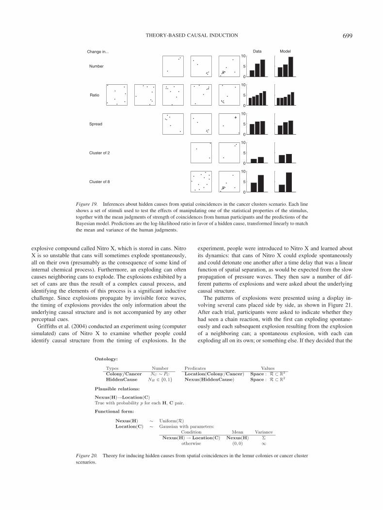
explosive compound called Nitro X, which is stored in cans. NitroX is so unstable that cans will sometimes explode spontaneously,all on their own (presumably as the consequence of some kind ofinternal chemical process). Furthermore, an exploding can oftencauses neighboring cans to explode. The explosions exhibited by aset of cans are thus the result of a complex causal process, andidentifying the elements of this process is a significant inductivechallenge. Since explosions propagate by invisible force waves,the timing of explosions provides the only information about theunderlying causal structure and is not accompanied by any otherperceptual cues.

Griffiths et al. (2004) conducted an experiment using (computersimulated) cans of Nitro X to examine whether people couldidentify causal structure from the timing of explosions. In the

experiment, people were introduced to Nitro X and learned aboutits dynamics: that cans of Nitro X could explode spontaneouslyand could detonate one another after a time delay that was a linearfunction of spatial separation, as would be expected from the slowpropagation of pressure waves. They then saw a number of dif-ferent patterns of explosions and were asked about the underlyingcausal structure.

The patterns of explosions were presented using a display in-volving several cans placed side by side, as shown in Figure 21.After each trial, participants were asked to indicate whether theyhad seen a chain reaction, with the first can exploding spontane-ously and each subsequent explosion resulting from the explosionof a neighboring can; a spontaneous explosion, with each canexploding all on its own; or something else. If they decided that the

0

5

10Data Model

Ratio

0

5

10

0

5

10

0

5

10

0

5

10

Change in...

Number

Spread

Cluster of 2

Cluster of 8

Figure 19. Inferences about hidden causes from spatial coincidences in the cancer clusters scenario. Each lineshows a set of stimuli used to test the effects of manipulating one of the statistical properties of the stimulus,together with the mean judgments of strength of coincidences from human participants and the predictions of theBayesian model. Predictions are the log-likelihood ratio in favor of a hidden cause, transformed linearly to matchthe mean and variance of the human judgments.

Figure 20. Theory for inducing hidden causes from spatial coincidences in the lemur colonies or cancer clusterscenarios.


explosion was the result of something else, they were asked towrite in a description of what they thought had happened. The firsttwo trials showed chain reactions. On the third trial, participantssaw the simultaneous explosion of several cans, as shown inFigure 21b, without the delays characteristic of pressure wavespropagating from one can to the next. The number of cans used inthe final trial was varied, to see whether this had an effect onpeople’s inferences.

Over 95% of participants correctly identified the causal chain inthe first two trials. For the third trial, the responses of people whochose the third option, that something other than a causal chain orspontaneous explosion had occurred, were coded by two raters.The proportion of participants identifying a hidden cause behindthe simultaneous explosion is shown in Figure 22. There was astatistically significant effect of NC: The number of cans influ-enced whether people inferred hidden causal structure, with mostpeople seeing two simultaneously exploding cans as independentbut six such cans as causally related. This provides a compellingillustration of the fact that people are able to infer hidden causesfrom small samples—in this case, only a single observation—aswell as a challenge for computational models: How might such aninference be explained?


We can explain people’s inferences about Nitro X within thetheory-based causal induction framework. There are two aspects ofthese inferences that require explanation: how people were able toidentify the causal structure as a chain reaction in the first two testtrials, and how they were able to infer a hidden cause in the thirdtest trial. Both of these aspects of human behavior can be ac-counted for as Bayesian inferences informed by the causal theorysketched in Figure 23. The ontology used in this theory has muchthe same structure as the theory for the stick-ball machine (seeFigure 16), with the key difference being that rather than having aset of discrete trials, the time at which events occur is a continuousquantity. There is also a connection between the plausible relationsand functional form assumed by the two theories, although thereare important differences that reflect the physical structure of thetwo systems.

The plausible relations identified by the theory are defined usingthe same schema as in the stick-ball theory, but they differ in theirprobabilities. For Nitro X, we know that the explosion of a can isable to cause the explosion of any other can, and that each can isable to explode spontaneously. As a consequence, links existbetween the ExplosionTime of any two cans and between the

ExplosionTime of each can and the ActivationTime of somehidden cause. As with the stick-ball theory, the hidden causeresponsible for each can is selected in proportion to the number ofother cans that are currently influenced by that cause.

The functional form assumed by the theory expresses the samequalitative commitments as the theory of the stick-ball machinebut translates these commitments into a domain where time iscontinuous. The ActivationTime of a hidden cause follows anexponential distribution with parameter , which is the continuouslimit of the case where a hidden cause activates on each trial withprobability , as in the stick-ball theory.15 The distribution of theExplosionTime of cans is similar to the movement of balls, exceptthat the causal relationship between cans is subject to a furtherconstraint: that there should be a delay between explosions com-mensurate with the distance between cans. As with the stick-balltheory, the assumptions of the Nitro X theory are consistent withthose of Newtonian physics: Cans do not explode without a causeand are likely to explode when such a cause manifests itself.

We use a continuous version of the noisy-OR to define thedistribution of the ExplosionTime of each can. The time at whichthe can explodes is assumed to be the time of the first arrival in anonhomogeneous Poisson process. This process defines some ratefunction �(t) indicating the mean rate of arrivals at each point intime t, with the probability of the first arrival occurring at time t�

being

P�first arrival at t�� t��exp��0

t�

��t�dt�, (9)

where the integral takes into account the probability of the eventnot occurring before time t�. We define the rate function of thePoisson process, �(t), to be a mixture of delta functions

15 Here, we assume that each hidden cause can become active only oncefor any set of cans. This is not a necessary assumption—Griffiths et al.(2004) explained these results using a model in which hidden causes couldhave multiple activations. This assumption produces the same qualitativepredictions as our account, but requires more complex mathematical anal-ysis. As with the stick-ball theory, it is also possible to allow multiplehidden causes to act on a single can.

(b)

(a)

Figure 21. Nitro X. (a) Four dormant cans, as displayed in the experimentdescribed in the text. (b) A simultaneous explosion.

2 3 4 60

0.2

0.4

0.6

0.8

1

Pro

babi

lity

of a

hid

den

caus

e

Number of cans

PeopleBayes

Figure 22. Causal induction from temporal coincidences. The proportionof people who identify the presence of a hidden cause increases with thenumber of cans that explode simultaneously, in accord with the predictionsof the theory-based Bayesian model (data from Griffiths et al., 2004).


��t� � �i

wi��t, ti�, (10)

where wi and ti are the weight and time associated with the ithcause, respectively. This formulation generalizes the noisy-OR, aseach cause has an independent opportunity to produce the effect(see Griffiths & Tenenbaum, 2005, for details).

The hypothesis space generated by this theory with NC � 4 isshown in Figure 24. The ActivationTime of a HiddenCause hi isindicated with a variable Hi, and the ExplosionTime of a Can ci

is indicated with a variable Ci. All cans can influence the explo-sions of other cans, in a generalization of the bidirectional rela-tionship between A and B shown in Graph 3 of the hypothesisspace for stick-balls (see Figure 17). Likewise, all cans are influ-enced by a hidden cause. The only difference between the graphsshown in Figure 24 is the configuration of the hidden causes,determining which cans will be correlated in their explosion times.The 15 graphs shown in the figure correspond to all partitions offour objects into different sets, where the objects are cans and allcans within a set share a hidden cause. The distribution over thesepartitions is provided by the Chinese restaurant process.

This theory can be used to explain how people are able toidentify the causal sequence responsible for a particular set ofexplosions. If we assume that s is much larger than 1, thenP(Graph 0) is greater than the probability of any other graph, andthe data provide only evidence in support of this conclusion.Consequently, to simplify our analysis we will outline how itproceeds just in Graph 0. Under this causal structure, the firstexplosion is always the consequence of a hidden cause becoming

active and is hence spontaneous. There are two possible explana-tions for each subsequent explosion occurring at a time appropriateto its distance from previous explosions: that it occurred sponta-neously, or that it was caused by those previous explosions. Underthis model a set of NC appropriately spaced explosions is muchmore probable under a causal chain than a spontaneous explosion(see Griffiths, 2005, Appendix D, for a detailed proof).

Identifying a set of explosions as the consequence of a singlehidden common cause requires evaluating the posterior distribu-tion over causal graphical models. In particular, it requires con-cluding that some structure other than Graph 0 is appropriate.Using the variable Cj to indicate the explosion time of the jth can,the theory in Figure 23 gives the probability of a simultaneousexplosion (Cj � t for all j, denoted C � t) under Graph i as

P�C � t�Graph i� � �NC� exp�� t��k,

where k is the number of hidden causes influencing cans in Graph i.The �NC results from the requirement that the NC cans all explodeat that moment, while the remainder of the expression is theprobability that the k hidden causes become active at that moment(and not before). Combining this probability with the prior definedby the theory, as shown in Figure 24, gives

P�Graph 0�C � t� ��NC

�j�0

NC�1

� j � ��

,

Figure 23. Theory for coincidences in explosion times. ExplosionTime(C) is the time at which can Cexplodes, and ActivationTime(H) the time at which a hidden cause becomes active. Cans can be causedto explode by the hidden causes or by the explosion of other cans. � is the rate at which force propagates fromone explosion to the next.


where � � s exp{� t}. This equation results from the fact thatGraph 0 requires NC hidden causes, and thus has posterior prob-ability proportional to (s exp{� t})NC, with the term in thedenominator being a normalizing constant for the resultingposterior distribution. The probability of the existence ofsome hidden cause, being 1 – P(Graph 0�C � t), increases asNC increases for any choice of s and , and using � � 12 producesthe predictions shown in Figure 22. These predictions correlatewith the experimental results at r � .97, with equivalently highcorrelations being produced for similar values of �.


Standard algorithms for learning causal graphical models cannotexplain these results. If we imagine that time is broken intodiscrete intervals, and a can either explodes or does not explode ineach interval, then we can construct a contingency table for eachpair of cans. Statistical significance tests will identify pairwisedependencies among all cans that explode simultaneously, pro-vided appropriate numbers of nonexplosion trials are included. Theexistence of a hidden common cause is consistent with such apattern of dependency. However, as a result of reasoning deduc-tively from this pattern, the evidence for such a structure does not

increase with NC: A hidden common cause is merely consistentwith the pattern for all NC � 2.

This experiment also illustrates that people are willing to inferhidden causal structure from very small samples—just one datapoint—and from observations alone. Standard constraint-basedalgorithms cannot solve this problem: While a hidden commoncause is consistent with the observed pattern of dependency, causalstructures in which the cans influence one another cannot be ruledout without intervention information. People do not consider thispossibility because they have learned that the mechanism by whichcans influence one another has a time delay.

Summary

The analyses presented in this section show how spatial andtemporal data can be incorporated into our formal framework,illustrated through consideration of how causal relationships canbe inferred from coincidences in space and time. Our theory-basedapproach makes it clear that these cases differ from causal induc-tion from contingency data only in the assumptions that they makeabout the functional form of causal relationships, allowing theserelationships to be expressed in spatial and temporal properties ofthe observed data as well as in the co-occurrence of cause and

1 2 3 4

1 2 3 4 1 2 3 4

H H

C C C C

32H 1

P(Graph 1) = s /(1+s)(2+s)(3+s) 2

1 2 3 4

H 1 H 2 H 3

1 2 3 4

H 1 H 2 H 3

1 2 3 4

H 1 H 2 H 3

C C C C

P(Graph 4) = s /(1+s)(2+s)(3+s) 2

1 2 3 4

H 1 H 3H 2

1 2 3 4

H 2

C C C C

H 1

P(Graph 7) = s/(1+s)(2+s)(3+s)

1 2 3 4

H 2H H

C C C C

31

P(Graph 2) = s /(1+s)(2+s)(3+s) 2

1 2 3 4

H 2

1 2 3 4

H 1 H 2

C C C C

P(Graph 9) = s/(1+s)(2+s)(3+s)

1 2 3 4

H 1 H 2

C C C C

P(Graph 10) = 2s/(1+s)(2+s)(3+s)

1 2 3 4

H 2H 1

C C C C

P(Graph 11) = 2s/(1+s)(2+s)(3+s)

1 2 3 4

H 1

1 2 3 4

H 2H 2 H 1

1 2 3 4

H 1

H H H H

C C C C

P(Graph 0) = s /(1+s)(2+s)(3+s) 3

C C C C

2P(Graph 3) = s /(1+s)(2+s)(3+s)

C C C C

P(Graph 5) = s /(1+s)(2+s)(3+s) 2

C C C C

2P(Graph 6) = s /(1+s)(2+s)(3+s)

H

C C C C

1

P(Graph 8) = s/(1+s)(2+s)(3+s)

C C C C

P(Graph 12) = 2s/(1+s)(2+s)(3+s)

C C C C

P(Graph 13) = 2s/(1+s)(2+s)(3+s)

C C C C

P(Graph 14) = 6/(1+s)(2+s)(3+s)

Figure 24. Hypothesis space for four cans of Nitro X. Ci indicates ExplosionTime(ci) for Can ci, while Hi

indicates ActivationTime(hi) for HiddenCause hi. The dependence of ExplosionTime(ci) on Explosion-Time(cj) and Position(ci) is suppressed. s indicates the tendency for cans to have unique hidden causes, asoutlined in the theory shown in Figure 23.


effect. By separating the elements of prior knowledge that influ-ence causal induction, we can emphasize those aspects that remainthe same—notions of causality, instantiated in causal graphicalmodels, and expectations about plausible causal structures—andidentify those aspects that differ.

The examples presented in this section address only the mostbasic questions about causal induction from spatial and temporaldata, and we hope to have the opportunity to test the predictions ofthese accounts further. The theories presented in each case makeinteresting new predictions. For example, the Nitro X theorypredicts that the evidence for a hidden common cause should begreater for a simultaneous explosion that occurs earlier. Thesepredictions deserve further investigation, as do more complexinstances of causal induction in dynamic physical systems, such asthose studied by Michotte (1963), which we have recently begunto address (Sanborn, Mansinghka, & Griffiths, 2006). In addition,we anticipate that the framework for modeling causal inductionfrom temporal data can be used to provide a deeper understandingof the recent results concerning the relationship between temporalcontiguity and contingency data that were summarized earlier inthis section (Buehner & May, 2002, 2003; Lagnado & Sloman,2006).

Causation Across Domains

We have presented a number of examples in which people’sintuitions about causal relationships can be explained as the resultof rational statistical inference applied to causal structures gener-ated by an appropriate causal theory. Since these theories expressknowledge relevant to a particular setting, we should expect thatthey will be domain sensitive, having content that is affected by thedomain in which causal inferences are made. In this section, weexamine how the influence of domain knowledge on causal induc-tion can be captured within our framework.

The definition of a domain is a problematic issue (e.g., Hir-schfeld & Gelman, 1994), but the term is commonly used to referto a set of phenomena that can be explained by appealing to acoherent set of causal principles. Physics, biology, and psychologyall involve quite different causal principles, such as force, growth,and desire. Even young children are sensitive to this variation,having different expectations about the causal relationships partic-ipated in by biological and nonbiological (Springer & Keil, 1991)and social and nonsocial (R. Gelman & Spelke, 1981; Shultz,1982a) entities. The early manifestation of domain-specific causalinferences, such as knowledge of the causal properties of objects(e.g., Spelke, Breinlinger, Macomber, & Jacobson, 1992), has ledto claims that these inferences are the result of distinct and spe-cialized cognitive modules (e.g., Leslie, 1994).

In attempting to formalize the content of intuitive theoriesrelevant to causal induction, we have the opportunity to considerhow the components of these theories might be affected by thedomain in which causal inferences are made. In particular, wemight expect that domain would have a strong influence on ex-pectations about functional form and the plausibility of causalrelationships. We consider how domain affects each of theseaspects of causal relationships in turn, using the analysis of exper-iments conducted by Schulz and Gopnik (2004) to support ourclaims.

The Effect of Domain on Functional Form

Causal relationships in different domains involve very differentcausal mechanisms. For example, you would probably use differ-ent methods to move a heavy box a foot to the left than to movea friend a foot to the left. However, this difference in the mecha-nism by which effects are brought about need not be reflected in adifference in the assumed functional form of the underlying rela-tionship. If attempting to drag a heavy box and asking your friendto move are both successful about 90% of the time, these tworelationships can be described by a similar functional form. Themapping from domain-specific mechanism to functional form ismany-to-one, with a variety of different mechanisms reducing tothe same set of qualitative assumptions about functional form.Consequently, causal induction involving systems in quite differ-ent domains can have much the same character: Even if the contentof theories differs, the constraints they imply for causal relation-ships can be the same.

An experiment conducted by Schulz and Gopnik (2004, Exper-iment 3) illustrates this point. In this experiment, children learnedabout causal relationships in two different domains: biology andpsychology. In the biology domain, children were asked to inferwhich flowers caused a toy monkey to sneeze, and in the psychol-ogy domain, they learned which animals scared a toy rabbit. Therewere two conditions in each domain. Using A, B, and C to indicatethe presence of each of three flowers (or animals) and E to indicatea sneezing monkey or a scared rabbit, the test condition consistedof four events: e��a�b�c�, e��a�b�c�, e��a�b�c�, ande��a�b�c�. The control condition featured four different events:e��a�b�c�, e��a�b�c�, e��a�b�c�, and e��a�b�c�. Childrenmade quite similar inferences across the two domains, as shown inTable 7, identifying C as the cause in the test condition, and all ofA, B, and C as causes in the control condition.

Schulz and Gopnik (2004) used the results of this experiment toargue that children’s ability to infer causal relationships is domainindependent. A different interpretation of these results is that theyindicate that the same functional form can be assumed in differentdomains (and for different underlying causal mechanisms). If thetheories characterizing two systems are isomorphic, then causalinferences using those theories will be identical. A pair of isomorphictheories for sneezing and scaring is shown in Figures 25 and 26.There is a direct correspondence between the types of entitiesidentified by these theories and the predicates applied to thoseentities, with Flower and Beast, Monkey and Rabbit, andSneezes and Scared all playing the same roles. The theories are

Table 7Effect of Domain on Functional Form

Condition C All Other

Test (biology) .78 (.90) .11 (.00) .11 (.10)Control (biology) .05 (.06) .89 (.86) .05 (.08)Test (psychology) .67 (.90) .28 (.00) .05 (.10)Control (psychology) .05 (.06) .83 (.86) .11 (.08)

Note. Numbers indicate the proportion of children identifying C as thecause, indentifying A, B, and C as causes, or producing some otherresponse, from Schulz and Gopnik (2004, Experiment 3). Predictions of theBayesian model are given in parentheses. Boldface values indicate major-ity.


identical in their assumptions about the plausibility of causalrelationships and the functional form of those relationships. For thestimuli shown to the children, both theories generate the samehypothesis space of causal graphical models.

Under the theories shown in Figures 25 and 26, the influences ofmultiple causes on both sneezing and scaring are described by thenoisy-OR parameterization. The use of the same functional formacross the two theories is a consequence of the applicability of thesame set of assumptions about the nature of causal relationships inthe domain: that causes influence their effects probabilistically,and that each of these influences has an independent opportunity todo so. This shared functional form results in the same predictionsfor the two conditions, as shown in Table 7. These predictions usedp � .5 and ε � .05 for both biology and psychology.

The Effect of Domain on Plausibility

In many of the examples discussed in the previous sections,assumptions about the plausibility of a causal relationship playeda less important role than assumptions about the underlying on-tology and the functional form of causal relationships. In part, this

is because the stimuli used in experiments on causal learning tendto involve variables among which causal relationships are quiteplausible. Studying problems of causal learning involving vari-ables from different domains provides an opportunity to explorethe effect of domain on the plausibility of causal relationships. Inparticular, one might expect that plausible relationships would berestricted to causes that use forces appropriate to that domain. Forexample, asking a box to move is far less likely to be successfulthan dragging it. Using examples similar to this, Schulz andGopnik (2004) have recently investigated how children assess theplausibility of causal relationships across domains and how thisassessment interacts with statistical evidence.

Schulz and Gopnik (2004, Experiment 4) introduced children tocausal systems in two domains. The physical domain involved amachine that made noise, with the candidate causes of the activa-tion of the machine being two magnetic buttons (the in-domainobjects a and b) and speech (the out-domain object c). Thepsychological domain involved reasoning about what might makea person giggle. The in-domain objects a and b were silly faces,and the out-domain object c was a switch. In each domain, children

Figure 25. Theory for causal induction with “biology” (sneezing monkeys).

Figure 26. Theory for causal induction with “psychology” (scared rabbits).


were first asked which objects were likely to produce the effect,and they unanimously identified the in-domain causes. They thensaw a series of trials exactly the same as those used in the testcondition of Schulz and Gopnik’s (2004) Experiment 3, discussedabove. As shown in Table 8, the majority of the children nowidentified the out-domain object c as the cause, despite its lowinitial plausibility.

A simple theory that characterizes both the physical and thepsychological stimuli used by Schulz and Gopnik (2004) is shownin Figure 27. Under this theory, both in-domain and out-domainobjects can influence the effect, but the plausibility of such rela-tionships differs. The probability of an in-domain relationship isset by p, while the probability of an out-domain relationship is setby q. The hypothesis space generated by this model for objects a,b, and c is functionally equivalent to that shown in Figure 12,using A to indicate the presence of a, B to indicate the presence ofb, C to indicate the presence of c, and E to indicate the activationof the effect.

The initial responses of the children in Schulz and Gopnik’s(2004) experiment indicates that q is much less than p. Thepredictions of the model with p � .4, q � .1, and ε � .1 are shownin Table 8. The model identifies c as a cause, despite its lowplausibility, because of the strong assumptions about functionalform. This effect can be best understood by considering the limitas ε3 0. If E never occurs in the absence of a cause, then seeingE occur in the presence of c provides unambiguous evidence thatC causes E. Thus, provided q takes on some value greater thanzero, the probability that C causes E will be 1.00. Allowing ε totake on values greater than zero increases the influence of q on theoutcome. In particular, if ε is somewhat greater than q, it becomesmore likely that A and B are causes of E, and the causal relation-ship simply failed to manifest on the trials when a and b werepresent.

Schulz and Gopnik (2004) interpreted this experiment as indi-cating that children are aware of domain-specific constraints oncausal relationships but that these constraints can be overridden bydomain-general principles of causal learning. In the analysisabove, the probability of an out-domain variable being involved ina causal relationship, q, has little effect on the predictions of themodel: The assumptions about the functional form of the causalrelationship mean that C will be identified as the cause even if q isvery small. The model predicts that the value of q would have agreater effect given ambiguous evidence. For example, seeinge��a�b�c� and e��a�b�c� would suggest that A and B cause Eif q is small, and that C causes E if q is large. Examining inferencesfrom ambiguous evidence thus provides an opportunity to explore

whether children really assign lower prior probability to cross-domain causal relationships.

Bonawitz, Griffiths, and Schulz (2006) tested the prediction thatambiguous evidence should trade off with priors based on domain,presenting preschoolers with ambiguous evidence involving eitherin-domain or cross-domain causes. The experiment was conductedwith 4- and 5-year-old children, who were assigned to either abaseline or an evidence condition. Children in both conditions sawboth within-domain and cross-domain storybooks. In the baselinecondition, the storybooks featured the events of a single day, inwhich a character interacted with two potential causes (a and b) ofan effect. For example, in the within-domain storybook, a deer ranin two places and got itchy spots. In the cross-domain story book,a bunny rabbit was scared (cause a) and ate something (cause b),then got a tummy ache. Children were then asked to select whichof the causes they thought was responsible for the effect. In theevidence condition, children saw 7 days in the life of the character,and one of the two causes (a) recurred on each day, together witha new potential cause each day. This provides ambiguous evidencethat a is the cause, as it is also possible that each of the seven otherpotential causes produces the effect. At the end of the story,children were asked which of the causes was responsible for theeffect. The results are shown in Figure 28 together with thepredictions of the theory-based Bayesian model outlined above,with p � .4 and q � .1 and ε � .001. Children’s responses matchthe qualitative predictions of this model, with the cross-domaincause initially being given less credence than the within-domaincause, but becoming increasingly acceptable as a result of theprovision of the ambiguous evidence. The model provides a rea-sonable quantitative match to the data, with r � .84, although themodel predicts a stronger effect of the ambiguous evidence thanwas observed with children. A replication of the cross-domaincondition (Experiment 2 of Schulz, Bonawitz, & Griffiths, 2007)found that 60% of children chose A, expressing a preference moreconsistent with that of the model. However, in general, childrenwere more conservative than the model predicts, being moreaffected by the prior and less affected than the data.

Summary

Different domains operate by different causal principles, a factthat can be captured in the theory-based framework by usingdifferent causal theories and by allowing relationships to differ intheir plausibility. However, such differences need not alwaysresult in different behavior: As shown by the results of Schulz andGopnik (2004, Experiment 3), if the theories that describe causalsystems in two domains imply the same constraints on causalgraphical models, then we should expect causal inferences to havemuch the same character across those systems. Likewise, whileknowledge of the causal principles by which different domainsoperate can influence the plausibility of causal relationships,strong assumptions about functional form can overwhelm theeffects of plausibility, as in Schulz and Gopnik (2004, Experiment4). These experiments thus leave open the possibility that domain-specific knowledge guides causal induction. Some support for thisidea is provided by subsequent experiments, which suggest thatcauses that cross domains are assigned lower prior probability(Bonawitz et al., 2006; Schulz et al., 2007).

Table 8Effect of Domain on Plausibility

Condition c a, b Other

Physical .75 (.72) .00 (.09) .25 (.19)Psychological .81 (.72) .00 (.09) .19 (.19)

Note. Numbers indicate the proportion of children identifying c as acause, identifying a and/or b as a cause, or producing some other response,from Schulz and Gopnik (2004, Experiment 4). Predictions of the Bayesianmodel are given in parentheses. Boldface values indicate majority.


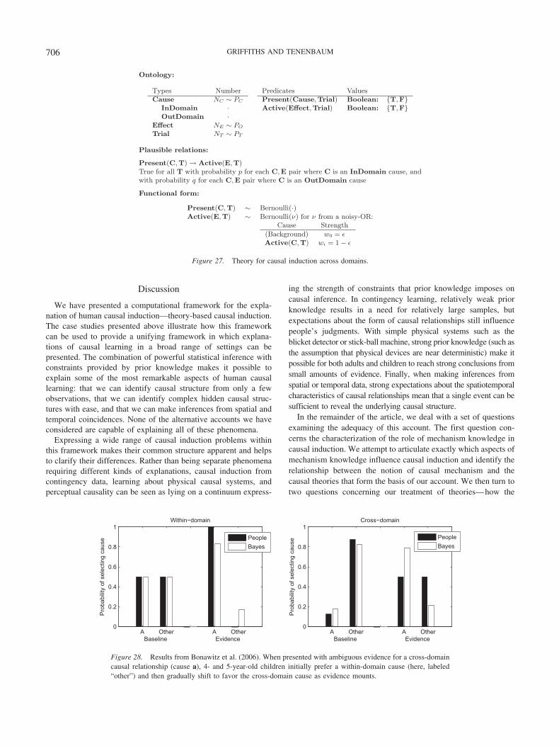
Discussion

We have presented a computational framework for the expla-nation of human causal induction—theory-based causal induction.The case studies presented above illustrate how this frameworkcan be used to provide a unifying framework in which explana-tions of causal learning in a broad range of settings can bepresented. The combination of powerful statistical inference withconstraints provided by prior knowledge makes it possible toexplain some of the most remarkable aspects of human causallearning: that we can identify causal structure from only a fewobservations, that we can identify complex hidden causal struc-tures with ease, and that we can make inferences from spatial andtemporal coincidences. None of the alternative accounts we haveconsidered are capable of explaining all of these phenomena.

Expressing a wide range of causal induction problems withinthis framework makes their common structure apparent and helpsto clarify their differences. Rather than being separate phenomenarequiring different kinds of explanations, causal induction fromcontingency data, learning about physical causal systems, andperceptual causality can be seen as lying on a continuum express-

ing the strength of constraints that prior knowledge imposes oncausal inference. In contingency learning, relatively weak priorknowledge results in a need for relatively large samples, butexpectations about the form of causal relationships still influencepeople’s judgments. With simple physical systems such as theblicket detector or stick-ball machine, strong prior knowledge (such asthe assumption that physical devices are near deterministic) make itpossible for both adults and children to reach strong conclusions fromsmall amounts of evidence. Finally, when making inferences fromspatial or temporal data, strong expectations about the spatiotemporalcharacteristics of causal relationships mean that a single event can besufficient to reveal the underlying causal structure.

In the remainder of the article, we deal with a set of questionsexamining the adequacy of this account. The first question con-cerns the characterization of the role of mechanism knowledge incausal induction. We attempt to articulate exactly which aspects ofmechanism knowledge influence causal induction and identify therelationship between the notion of causal mechanism and thecausal theories that form the basis of our account. We then turn totwo questions concerning our treatment of theories—how the

Figure 27. Theory for causal induction across domains.

A Other A Other0

0.2

0.4

0.6

0.8

1Within−domain

Pro

babi

lity

of s

elec

ting

caus

e

Baseline EvidenceA Other A Other

0

0.2

0.4

0.6

0.8

1Cross−domain

Pro

babi

lity

of s

elec

ting

caus

e

Baseline Evidence

PeopleBayes

PeopleBayes

Figure 28. Results from Bonawitz et al. (2006). When presented with ambiguous evidence for a cross-domaincausal relationship (cause a), 4- and 5-year-old children initially prefer a within-domain cause (here, labeled“other”) and then gradually shift to favor the cross-domain cause as evidence mounts.


relatively low-level theories that we have discussed can be ex-tended and how such theories might be learned—before brieflyconsidering the kinds of psychological processes that might sup-port rational theory-based causal induction.

Causal Mechanisms and Causal Theories

As mentioned at the start of the article, psychological theoriesabout causal induction have traditionally fallen into two camps(Newsome, 2003): Covariation-based approaches characterize hu-man causal induction as the consequence of a domain-generalstatistical sensitivity to covariation between cause and effect (e.g.,Cheng & Novick, 1990, 1992; Shanks & Dickinson, 1987),whereas mechanism-based approaches focus on the role of priorknowledge about the mechanisms by which causal force can betransferred (e.g., Ahn & Kalish, 2000; Shultz, 1982b; White,1995). Recently, these two approaches have begun to be broughttogether through theories that consider how prior knowledge canbe combined with covariational evidence (Koslowski, 1996; Wald-mann, 1996; Waldmann et al., 2006). Our theory-based approachformalizes the interaction between prior knowledge and statisticallearning in causal induction. In this section we attempt to clarifyhow the theory-based prior knowledge appealed to by our ap-proach connects to the notion of causal mechanism.

When researchers refer to causal mechanism, they typicallymean the chain of events mediating between cause and effect, asillustrated in Figure 29a (e.g., Bullock et al., 1982; Glymour, &Cheng, 1998; Shultz, Pardo, & Altmann, 1982; see Shultz &Kestenbaum, 1985, for a discussion of different kinds of mecha-nism). However, a detailed understanding of the mechanismsmediating between cause and effect is clearly not necessary forcausal induction—if one possessed such knowledge there wouldbe nothing to learn. Furthermore, recent studies investigating thelimits of people’s understanding of causal systems suggests that infact, our mechanism knowledge may look more like Figure 29b.For example, Rozenblit and Keil (2002) found that when asked toexplain how mechanical systems like crossbows and helicopterswork, people radically overestimated the extent of their mecha-nism knowledge. It seems that, in general, our causal knowledgeidentifies the fact that a mechanism exists but does not necessarilyarticulate all of the steps that connect cause and effect (Keil, 2003).

Results like those of Rozenblit and Keil (2002) raise an inter-esting question: If our knowledge of causal mechanisms is asshallow as it appears to be, how is it possible for this knowledgeto inform causal induction? Our theory-based account provides ananswer to this question. Under our account, prior knowledge playstwo important roles in causal induction: identifying which relation-

ships are plausible and characterizing the functional form of thoserelationships. The shallow mechanism knowledge described by Keil(2003) is sufficient to fulfill these roles. Whether a causal relationshipseems plausible is affected by mechanism knowledge, but the keydeterminant in this decision is not the particular details of the causalmechanism, but whether such a mechanism could exist. Similarly,evaluating the functional form of a causal relationship does notrequire knowing every step between cause and effect, but knowingwhat kind of relationship those steps might produce.

Neither assessing plausibility nor specifying functional formrequires a detailed account of a chain of events from cause toeffect. As mentioned previously, a number of studies have sug-gested that simply believing a mechanism could exist makes acausal relationship seem more plausible (Koslowski, 1996;Koslowski & Okagaki, 1986; Koslowski et al., 1989). Lack of com-plete mechanism knowledge is likewise no impediment to reasoningabout the functional form of a causal relationship. This point isillustrated through our use of Halley’s inference as an example of acase in which prior knowledge guided causal induction. Newton’stheory was notoriously amechanistic, departing from its forebears byintroducing forces unmediated by particles (e.g., Westfall, 1977).Physicists are still engaged in the project of providing a mechanisticaccount of Newton’s ideas, and in particular the force of gravity.Although Halley did not know the means by which the masses of starsand planets influenced the orbits of comets, he was still able to useinformation about the form of this influence to reason about the causeof the events that he observed. Indeed, in introducing his own accountof causality, Pearl (1996) reduced mechanisms to “nothing but ordi-nary physical laws, cast in the form of deterministic equations”(p. 432), being no more than the specification of the functional formof the relationship between two variables.

The causal theories used in theory-based causal induction canthus be viewed as expressing the consequences of the shallowknowledge people possess of the mechanisms that operate indifferent domains. However, these theories do not express thatknowledge directly: They are just as amechanistic as Newton’stheory of physics, characterizing the possible relationships amongentities and their form. The theories we have described are theconstraints on the functional relationships among variables thatcan be the consequence of mechanism knowledge rather than theknowledge itself. Many mechanisms can imply the same set ofconstraints, as illustrated in the discussion of domain specificity inthe previous section.

Distinguishing between theories and mechanisms provides animportant insight into how causal induction is possible. A majorchallenge for mechanism-based accounts of causal induction isexplaining how new causal mechanisms might be learned: If allcausal induction requires mechanism knowledge, one can neverdiscover a relationship that suggests a new mechanism (e.g.,Cheng, 1993). If theory and mechanism are distinct, it becomespossible to learn a set of causal relationships without knowing theirunderlying mechanism. The existence of these relationships canthen encourage the search for a mechanism that accounts for them,and the discovery of such a mechanism justifies further inferencesabout possible causal relationships. Such a pattern is extremelycommon in science—most of the suspicious coincidences thatsuggest new causal relationships are followed by a search for anexplanatory mechanism (cf. Griffiths & Tenenbaum, 2007a).

C(b) E1M M2 M?. . .

(a) EC 1M M2 M?. . .

Figure 29. Two conceptions of causal mechanism knowledge. (a) Thecausal mechanism specifies the chain of events mediating between cause Cand its effect E. (b) Often, people know that some mechanism (M) exists,but not the details.


Higher Level Causal Theories

The causal theories that we have used throughout this article havethe same constituents as the intuitive theories discussed in accounts ofcognition and cognitive development—ontologies and causal laws—but are far more limited in scope. Our analogy to Wellman’s (1990;Wellman & Gelman, 1992) notion of a framework theory is useful inindicating the way that multiple levels of causal knowledge interact,but misleading in suggesting that the causal theories we describe areat the same level of generality as framework theories. Frameworktheories are supposed to provide the fundamental principles used inorganizing an entire domain, such as intuitive physics, biology, orpsychology. The theories we have presented characterize the princi-ples that underlie very simple causal systems, with well-delineatedboundaries. Although our theory of Nitro X makes predictions for anyarray of arbitrarily many cans of explosive, it hardly provides acomplete theory of all physical systems.

The theories described in the article constitute the lowest levelof causal theory, identifying the causal principles involved inspecific kinds of systems. Doing justice to the notion of a frame-work theory requires postulating the existence of higher leveltheories, which express principles common to many systems.Following our definition of theories as hypothesis space genera-tors, these higher level theories should generate hypothesis spacesthat consist of different theories of particular causal systems (Te-nenbaum et al., 2007). As discussed in the next section, suchhypothesis spaces can be used to determine which theory bestcharacterizes the forces at work in a system.

Identifying the kind of principles that should be included in thesehigher level theories requires investigating the assumptions that guidecausal induction across a wide range of systems. By examininginferences involving different systems in physics, biology, and psy-chology, it should become possible to pick out the domain-specificprinciples that generate the theories of these systems that people use.Our investigation of different physical systems, such as the stick-ballmachine and Nitro X, suggests what some of these principles might befor the domain of physics. The theories that we used to explainpeople’s inferences about these systems had much the same character,using hidden causes ( prime movers) to inject mechanical energy intothe system, and having rules stating that no object changes statewithout a cause, and that causes produce changes in state with highprobability. These principles may be a part of the higher level theorythat organizes knowledge about all physical systems, constituting apart of our intuitive physics.

Learning Causal Theories

We have argued that human causal induction—the inference tocausal structure from data—can be viewed as the result of a statis-tical inference comparing hypotheses generated by a causal theory.This approach explains how people are able to infer causal relation-ships from small samples and identify complex causal structures.However, it raises a new problem: explaining how people learn causaltheories.

Our account of how people learn causal theories will generallyhave the same character as our account of how people learn causalstructure. As stated above, the three levels of representation used inour account—theories, hypotheses, and data—and the assumptionthat each level generates the one below define a hierarchical Bayesian

model (Tenenbaum et al., 2006). This model can be used to makeinferences about any level in the hierarchy. As mentioned in ourdiscussion of the blicket detector, the data D can be used to makeinferences about the theory T—this just requires applying Bayes’ ruleat the level of theories (Equation 8). However, in the case of theblicket detector, there were only two theories to compare. In general,the problem of learning a theory is much more complex.

Applying Bayes’ rule at the level of theories, T, requires having aprior distribution over such theories, P(T). Just as people have strongexpectations about the causal relationships that might hold in a givensystem, they have strong expectations about the kind of causal rela-tionships that could operate in a domain. For example, theories of thestick-ball machine are constrained by beliefs about how any physicalsystem could work. These constraints are expressed in higher leveldomain theories. Assuming that such higher level theories generatetheories of particular systems, such higher level theories provide ahypothesis space of theories, T, and a prior on those theories.

Developing and testing this account of how theories are learnedprovides an important direction for future research. Our discussion ofthe blicket detector example illustrates how people might learn thefunctional form of a causal relationship, showing that assumptionsabout deterministic relationships can be easily overruled. Empiricalinvestigation of the predictions of this account would reveal whetherpeople’s judgments can change in the same way. The question of howtypes of entities might be inferred, and how this interacts with plau-sibility, has recently been explored by Tenenbaum and Niyogi (2003),who showed that people could learn about the existence of differenttypes of entities purely on the basis of the causal relationships inwhich they participated. Kemp, Griffiths, and Tenenbaum (2004)have developed a computational model that explains how such learn-ing can take place, using Bayesian inference to simultaneously iden-tify the number of types, the types themselves, and the plausibility ofcausal relationships among entities of those types, and Kemp et al.(2007) showed how this approach could be applied to human learningof simple theories.

Providing an account of how people learn causal theories ofspecific systems that appeals to higher level causal theories raisesa new problem: explaining how these higher level theories arelearned. Changes in the causal theories of domains constitute someof the most interesting phenomena in cognitive development, andin the history of science. However, at this point, concerns about aninfinite recursion, providing no ultimate solution to the question ofhow people learn causal relationships, seem justified. There arethree reasons not to be concerned by such a recursion. First, themechanism by which the inference is performed at each step is thesame—regardless of the level of representation, inferences aboutthe level above can be made using Bayesian inference. There isthus no mysterious new force of learning that enters at any point.Second, this inference can become simpler at each level, withpotentially fewer hypotheses about the more abstract principlesthat organize a domain, and a broader range of observed data thatprovide information about those principles. Third, the recursion isnot infinite. At some point, it grounds out in a set of basicassumptions about the nature of causality, which provide con-straints on the most general domain theories. Some of the impli-cations of this idea of a recursive hierarchy of causal theories areexplored in Tenenbaum et al. (2007).


Psychological Mechanisms Supporting Rational CausalInduction

Our focus in this article has been on providing a computational-level analysis of causal induction, rather than an account of therepresentations and algorithms that people use to solve this problem,or the way in which those representations and algorithms are imple-mented. However, Marr’s (1982) levels of analysis were not intendedto be completely independent, with constraints from the differentlevels influencing one another. In this case, we can ask what con-straints our computational-level analysis might impose on the kinds ofpsychological processes we might expect to support causal induction.

The most fundamental question that our analysis raises is that ofhow human minds might even be capable of performing the kindof computations that are involved in the models of causal inductionthat we have considered. The number of causal graphical modelsthat can be expressed using a given set of variables grows expo-nentially in the number of variables, and the computational cost ofperforming Bayesian inference increases linearly with the size ofthe hypothesis space. Consequently, it would seem that we wouldrapidly run into serious computational limitations in the kind ofcausal learning we might expect people to be able to perform.

Our answer to this problem comes in two parts. The first part isbuilt into our framework, through the idea that theories provideconstraints on causal learning. These constraints effectively reducethe size of the hypothesis space involved in causal learning—something that makes it easier to learn from small amounts of data,but that also reduces the amount of computation required inlearning. As we have argued throughout the article, the strongconstraints provided by prior knowledge are the key to why peopleare so good at causal induction. Indeed, recent work in machinelearning has begun to explore ways of constraining hypothesesabout causal structure in order to be able to learn from smalleramounts of data and to do so with less computation (e.g., Segal,Pe’er, et al., 2003; Segal, Shapira, et al., 2003).

In considering the psychological plausibility of this kind of con-strained combinatorial computation, it is worth returning to our lin-guistic analogy. Under a standard (generative grammar inspired)account of sentence processing, when people hear a sentence theymake an inference about the syntactic structure underlying the wordsin the sentence. This is exactly the same kind of computation as weare proposing the human mind performs in causal learning: The spaceof possible syntactic structures increases exponentially in the length ofthe sentence, and the grammar provides constraints that combine withthe words to yield the most likely interpretation. If people can inter-pret sentences, even doing so online, in a way that is robust tointerference, then they have all the computational resources requiredto perform theory-based causal induction.

The second part of our answer is that we expect the mind not tobe performing all of the computations required for Bayesian in-ference but to be using an efficient approximation. One source ofheuristic approximations for the kind of computations involved incausal inference is Monte Carlo simulation: rather than consider-ing all possible hypotheses, considering a randomly generatedsubset. Monte Carlo techniques are commonly used in the machinelearning literature on learning the structure of graphical models(e.g., Friedman & Koller, 2000) and can also be found in solutionsto the problem of statistical parsing we have been using in ouranalogy (e.g., Johnson, Griffiths, & Goldwater, 2007). In particu-

lar, a technique known as a particle filter provides a way tomaintain only a finite number of hypotheses over time, updatingthose hypotheses as new data become available in order to approx-imate the new posterior distribution (Doucet, Freitas, & Gordon,2001). Particle filters have been proposed as psychological modelsin other settings, including categorization (Sanborn, Griffiths, &Navarro, 2006), change detection (Brown & Steyvers, 2009), andsentence processing (Levy, Reali, & Griffiths, 2009).

We remain agnostic about the specific psychological processesunderlying causal induction and open to proposals of ways inwhich simple heuristics and associative learning might be used toapproximate the statistical computations at the heart of our ac-count. However, our computational-level analysis provides clearlyspecified goals for what such algorithms and representationsshould aim to approximate, and we suspect that considering strat-egies for approximating these computations will provide a produc-tive means of generating hypotheses about psychological mecha-nisms that could support rational theory-based causal induction.

Conclusion

The human ability to infer causal structure from observed data hastraditionally been studied in several very different settings, withcorrespondingly different kinds of cognitive capacities invoked toexplain this ability. Causal learning from contingency data has beenviewed as the result of associative learning or intuitive statisticalreasoning processes. Learning about causality in simple physicalsystems has been explained in terms of mechanistic reasoning. De-tecting hidden causal structure in patterns of spatial and temporalcoincidence has been attributed to innate, modular perceptual pro-cesses. However, all of these different species of causal inductionhave at their heart the same computational problem, which suggestscommon principles by which they might operate.

The common challenge is the classic problem of induction: to inferthe true causal relations that hold among a set of events, given a smallfinite set of observations that could have been produced by (and henceare logically consistent with) many possible causal structures. Thisproblem can be approached as a statistical inference, but learningfrom small amounts of data can be successful only if constrained bystrong and appropriate prior knowledge. We have argued that in orderto capture the background knowledge that guides human causal learn-ing, we need a representational framework that is richer and moreabstract than the language of causal graphical models or Bayesiannetworks that has recently become influential in psychology. We haveshown how to formalize causal background knowledge in terms ofprobabilistic logical theories and shown how such theories can beintegrated with a Bayesian framework for causal learning. The theorygenerates a hypothesis space of candidate causal structures that couldexplain a set of observed data, along with a prior distribution overthose hypotheses which serves to favor some candidate explanationsover others.

We have applied our theory-based approach to a number of casestudies in causal induction, covering a broad range of differentkinds of causal systems, and a variety of settings in which peoplelearn about causal relationships. Learning in each of these settingscan be explained as a Bayesian inference constrained by a differentcausal theory. The variation in human judgments across settingsprovides insight into the roles that background knowledge plays inguiding human causal learning: As background knowledge be-


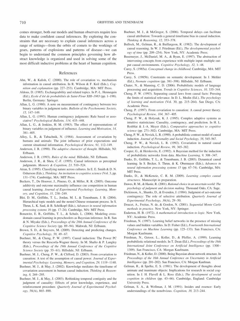
comes stronger, both our models and human observers require lessdata to make confident causal inferences. By exploring the con-straints that are necessary to explain causal inferences across arange of settings—from the orbits of comets to the workings ofgears, patterns of explosions and patterns of disease—we canbegin to understand the common principles governing how ab-stract knowledge is organized and used in solving some of themost difficult inductive problems at the heart of human cognition.

References

Ahn, W., & Kalish, C. (2000). The role of covariation vs. mechanisminformation in causal attribution. In R. Wilson & F. Keil (Eds.), Cog-nition and explanation (pp. 227–253). Cambridge, MA: MIT Press.

Aldous, D. (1985). Exchangeability and related topics. In P.-L. Hennequin(Ed.), Ecole d’ete de probabilites de Saint-Flour XIII–1983 (pp. 1–198).Berlin, Germany: Springer.

Allan, L. G. (1980). A note on measurement of contingency between twobinary variables in judgment tasks. Bulletin of the Psychonomic Society,15, 147–149.

Allan, L. G. (1993). Human contingency judgments: Rule based or asso-ciative? Psychological Bulletin, 114, 435–448.

Allan, L. G., & Jenkins, H. M. (1983). The effect of representations ofbinary variables on judgment of influence. Learning and Motivation, 14,381–405.

Alloy, L. B., & Tabachnik, N. (1984). Assessment of covariation byhumans and animals: The joint influence of prior expectations andcurrent situational information. Psychological Review, 91, 112–149.

Anderson, J. R. (1990). The adaptive character of thought. Hillsdale, NJ:Erlbaum.

Anderson, J. R. (1993). Rules of the mind. Hillsdale, NJ: Erlbaum.Anderson, J. R., & Sheu, C.-F. (1995). Causal inferences as perceptual

judgments. Memory & Cognition, 23, 510–524.Atran, S. (1995). Classifying nature across cultures. In E. E. Smith & D. N.

Osherson (Eds.), Thinking: An invitation to cognitive science (Vol. 3, pp.131–174). Cambridge, MA: MIT Press.

Beckers, T., De Houwer, J., Pineno, O., & Miller, R. R. (2005). Outcomeadditivity and outcome maximality influence cue competition in humancausal learning. Journal of Experimental Psychology: Learning, Mem-ory, and Cognition, 31, 238–249.

Blei, D. M., Griffiths, T. L., Jordan, M. I., & Tenenbaum, J. B. (2004).Hierarchical topic models and the nested Chinese restaurant process. In S.Thrun, L. K. Saul, & B. Scholkopf (Eds.), Advances in neural informationprocessing systems 16 (pp. 17–24). Cambridge, MA: MIT Press.

Bonawitz, E. B., Griffiths, T. L., & Schulz, L. (2006). Modeling cross-domain causal learning in preschoolers as Bayesian inference. In R. Sun& N. Miyake (Eds.), Proceedings of the 28th Annual Conference of theCognitive Science Society (pp. 89–94). Mahwah, NJ: Erlbaum.

Brown, S. D., & Steyvers, M. (2009). Detecting and predicting changes.Cognitive Psychology, 58, 49–67.

Buehner, M., & Cheng, P. W. (1997). Causal induction: The Power PCtheory versus the Rescorla-Wagner theory. In M. Shafto & P. Langley(Eds.), Proceedings of the 19th Annual Conference of the CognitiveScience Society (pp. 55–61). Hillsdale, NJ: Erlbaum.

Buehner, M. J., Cheng, P. W., & Clifford, D. (2003). From covariation tocausation: A test of the assumption of causal power. Journal of Exper-imental Psychology: Learning, Memory, and Cognition, 29, 1119–1140.

Buehner, M. J., & May, J. (2002). Knowledge mediates the timeframe ofcovariation assessment in human causal induction. Thinking & Reason-ing, 8, 269–295.

Buehner, M. J., & May, J. (2003). Rethinking temporal contiguity and thejudgment of causality: Effects of prior knowledge, experience, andreinforcement procedure. Quarterly Journal of Experimental Psychol-ogy, 56(A), 865–890.

Buehner, M. J., & McGregor, S. (2006). Temporal delays can facilitatecausal attribution: Towards a general timeframe bias in causal induction.Thinking & Reasoning, 12, 353–378.

Bullock, M., Gelman, R., & Baillargeon, R. (1982). The development ofcausal reasoning. In W. J. Friedman (Ed.), The developmental psychol-ogy of time (pp. 209–254). New York, NY: Academic Press.

Busemeyer, J., McDaniel, M. A., & Byun, E. (1997). The abstraction ofintervening concepts from experience with multiple input–multiple out-put causal environments. Cognitive Psychology, 32, 1–48.

Carey, S. (1985a). Conceptual change in childhood. Cambridge, MA: MITPress.

Carey, S. (1985b). Constraints on semantic development. In J. Mehler(Ed.), Neonate cognition (pp. 381–398). Hillsdale, NJ: Erlbaum.

Chater, N., & Manning, C. D. (2006). Probabilistic models of languageprocessing and acquisition. Trends in Cognitive Sciences, 10, 335–344.

Cheng, P. W. (1993). Separating causal laws from causal facts: Pressingthe limits of statistical relevance. In D. L. Medin (Ed.), The psychologyof learning and motivation (Vol. 30, pp. 215–264). San Diego, CA:Academic Press.

Cheng, P. (1997). From covariation to causation: A causal power theory.Psychological Review, 104, 367–405.

Cheng, P. W., & Holyoak, K. J. (1995). Complex adaptive systems asintuitive statisticians: Causality, contingency, and prediction. In H. L.Roitblat & J.-A. Meyer (Eds.), Comparative approaches to cognitivescience (pp. 271–302). Cambridge, MA: MIT Press.

Cheng, P. W., & Novick, L. R. (1990). A probabilistic contrast model of causalinduction. Journal of Personality and Social Psychology, 58, 545–567.

Cheng, P. W., & Novick, L. R. (1992). Covariation in natural causalinduction. Psychological Review, 99, 365–382.

Cooper, G., & Herskovits, E. (1992). A Bayesian method for the inductionof probabilistic networks from data. Machine Learning, 9, 308–347.

Danks, D., Griffiths, T. L., & Tenenbaum, J. B. (2003). Dynamical causallearning. In S. Becker, S. Thrun, & K. Obermayer (Eds.), Advances inneural information processing systems 15 (pp. 67–74). Cambridge, MA:MIT Press.

Danks, D., & McKenzie, C. R. M. (2009). Learning complex causalstructures. Manuscript in preparation.

Dawes, R. M., & Hastie, R. (2001). Rational choice in an uncertain world: Thepsychology of judgment and decision making. Thousand Oaks, CA: Sage.

Dickinson, A., Shanks, D., & Evenden, J. (1984). Judgment of act-outcomecontingency: The role of selective attribution. Quarterly Journal ofExperimental Psychology, 36(A), 29–50.

Doucet, A., Freitas, N. de, & Gordon, N. (2001). Sequential Monte Carlomethods in practice. New York, NY: Springer.

Enderton, H. B. (1972). A mathematical introduction to logic. New York,NY: Academic Press.

Friedman, N. (1997). Learning belief networks in the presence of missingvalues and hidden variables. In D. Fisher (Ed.), Fourteenth InternationalConference on Machine Learning (pp. 125–133). San Francisco, CA:Morgan Kaufmann.

Friedman, N., Getoor, L., Koller, D., & Pfeffer, A. (1999). Learningprobabilistic relational models. In T. Dean (Ed.), Proceedings of the 16thInternational Joint Conference on Artificial Intelligence (pp. 1300–1309). San Francisco, CA: Morgan Kaufmann.

Friedman, N., & Koller, D. (2000). Being Bayesian about network structure. InProceedings of the 16th Annual Conference on Uncertainty in ArtificialIntelligence (pp. 201–202). San Francisco, CA: Morgan Kaufman.

Gelman, R., & Spelke, E. S. (1981). The development of thoughts aboutanimate and inanimate objects: Implications for research in social cog-nition. In J. H. Flavell & L. Ross (Eds.), The development of socialcognition in children (pp. 43–66). Cambridge, England: CambridgeUniversity Press.

Gelman, S. A., & Wellman, J. M. (1991). Insides and essence: Earlyunderstandings of the nonobvious. Cognition, 38, 213–244.


Glymour, C. (1998). Learning causes: Psychological explanations of causalexplanation. Minds and Machines, 8, 39–60.

Glymour, C. (2001). The mind’s arrows: Bayes nets and graphical causalmodels in psychology. Cambridge, MA: MIT Press.

Glymour, C., & Cheng, P. W. (1998). Causal mechanism and probability: Anormative approach. In M. Oaksford & N. Chater (Eds.), Rational models ofcognition (pp. 295–313). Oxford, England: Oxford University Press.

Gopnik, A. (1996). The scientist as child. Philosophy of Science, 63,485–514.

Gopnik, A., & Glymour, C. (2002). Causal maps and Bayes nets: Acognitive and computational account of theory-formation. In P. Carruth-ers, S. Stich, & M. Segal (Eds.), The cognitive basis of science. Cam-bridge, England: Cambridge University Press.

Gopnik, A., Glymour, C., Sobel, D., Schulz, L., Kushnir, T., & Danks, D.(2004). A theory of causal learning in children: Causal maps and Bayesnets. Psychological Review, 111, 1–31.

Gopnik, A., & Meltzoff, A. N. (1997). Words, thoughts, and theories.Cambridge, MA: MIT Press.

Gopnik, A., & Sobel, D. (2000). Detecting blickets: How young childrenuse information about novel causal powers in categorization and induc-tion. Child Development, 71, 1205–1222.

Gopnik, A., Sobel, D. M., Schulz, L. E., & Glymour, C. (2001). Causallearning mechanisms in very young children: Two-, three-, and four-year-olds infer causal relations from patterns of variation and covaria-tion. Developmental Psychology, 37, 620–629.

Greville, W. J., & Buehner, M. J. (2007). The influence of temporaldistributions on causal induction from tabular data. Memory & Cogni-tion, 35, 444–453.

Griffiths, T. L. (2005). Causes, coincidences, and theories. Unpublisheddoctoral dissertation, Stanford University.

Griffiths, T. L., Baraff, E. R., & Tenenbaum, J. B. (2004). Using physicaltheories to infer hidden causal structure. In K. Forbus, D. Gentner, & T.Regier (Eds.), Proceedings of the 26th Annual Conference of the Cog-nitive Science Society (pp. 446–451). Mahwah, NJ: Erlbaum.

Griffiths, T. L., & Ghahramani, Z. (2005). Infinite latent feature models andthe Indian buffet process (Tech. Rep. No. 2005–001). Gatsby Computa-tional Neuroscience Unit, University College London, England.

Griffiths, T. L., Sobel, D. M., Tenenbaum, J. B., & Gopnik, A. (2009).Bayes and blickets: Effects of knowledge on causal induction in childrenand adults. Manuscript submitted for publication.

Griffiths, T. L., & Tenenbaum, J. B. (2005). Structure and strength incausal induction. Cognitive Psychology, 51, 354–384.

Griffiths, T. L., & Tenenbaum, J. B. (2007a). From mere coincidences tomeaningful discoveries. Cognition, 103, 180–226.

Griffiths, T. L., & Tenenbaum, J. B. (2007b). Two proposals for causalgrammars. In A. Gopnik & L. Schulz (Eds.), Causal learning: Psychol-ogy, philosophy, and computation (pp. 323–346). Oxford, England:Oxford University Press.

Hagmayer, Y., Sloman, S. A., Lagnado, D. A., & Waldmann, M. R. (2007).Causal reasoning through intervention. In A. Gopnik & L. Schulz (Eds.),Causal learning: Psychology, philosophy, and computation (pp. 86–100). Oxford, England: Oxford University Press.

Hagmayer, Y., & Waldmann, M. R. (2002). How temporal assumptionsinfluence causal judgments. Memory & Cognition, 30, 1128–1137.

Hagmayer, Y., & Waldmann, M. R. (2007). Inferences about unobservedcauses in human contingency learning. Quarterly Journal of Experimen-tal Psychology, 60, 330–355.

Hattori, M., & Oaksford, M. (2007). Adaptive noninterventional heuristicsfor covariation detection in causal induction: Model comparison andrational analysis. Cognitive Science, 31, 765–814.

Heckerman, D. (1998). A tutorial on learning with Bayesian networks. InM. I. Jordan (Ed.), Learning in graphical models (pp. 301–354). Cam-bridge, MA: MIT Press.

Hirschfeld, L. A., & Gelman, S. A. (Eds.). (1994). Mapping the mind:

Domain specificity in cognition and culture. Cambridge, England: Cam-bridge University Press.

Holland, J. H., Holyoak, K. J., Nisbett, R. E., & Thagard, P. R. (1986).Induction: Processes of inference, learning and discovery. Cambridge,MA: MIT Press.

Hughes, D. W. (1990). Edmond Halley: His interest in comets. In N. J. M.Thrower (Ed.), Standing on the shoulders of giants: A longer view ofNewton and Halley (pp. 324–372). Los Angeles, CA: University ofCalifornia Press.

Hume, D. (1977). An enquiry concerning human understanding. Indianap-olis, IN: Hackett. (Original work published 1748)

Hume, D. (1978). A treatise of human nature. Oxford, England: OxfordUniversity Press. (Original work published 1739)

Humphreys, P., & Freedman, D. A. (1996). The grand leap. British Journalof the Philosophy of Science, 47, 113–123.

Inagaki, K., & Hatano, G. (2002). Young children’s thinking about bio-logical world. New York, NY: Psychology Press.

Inhelder, B., & Piaget, J. (1958). The growth of logical thinking fromchildhood to adolescence. London, England: Routledge and Kegan Paul.

Jenkins, H. M., & Ward, W. C. (1965). Judgment of contingency betweenresponses and outcomes. Psychological Monographs, 79.

Johnson, M., Griffiths, T. L., & Goldwater, S. (2007). Bayesian inferencefor PCFGs via Markov chain Monte Carlo. In Proceedings of the NorthAmerican Conference on Computational Linguistics (pp. 139–146).Rochester, NY: Association for Computational Linguistics.

Kant, I. (1964). Critique of pure reason. London, England: Macmillan.(Original work published 1781)

Karmiloff-Smith, A. (1988). The child is a theoretician, not an inductivist.Mind and Language, 3, 183–195.

Keil, F. C. (1989). Concepts, kinds, and cognitive development. Cam-bridge, MA: MIT Press.

Keil, F. C. (2003). Folkscience: Coarse interpretations of a complex reality.Trends in Cognitive Sciences, 7, 368–373.

Kelley, H. H. (1973). The processes of causal attribution. American Psy-chologist, 28, 107–128.

Kemp, C., Goodman, N. D., & Tenenbaum, J. B. (2007). Learning causalschemata. In D. McNamara & G. Trafton (Eds.), Proceedings of the 29thAnnual Conference of the Cognitive Science Society (pp. 389–394). NewYork, NY: Erlbaum.

Kemp, C., Griffiths, T. L., & Tenenbaum, J. B. (2004). Discovering latentclasses in relational data (AI Memo 2004–019). Cambridge, MA:Massachusetts Institute of Technology.

Kersting, K., & De Raedt, L. (2000). Bayesian logic programs. In J.Cussens & A. Frisch (Eds.), Proceedings of the work-in-progress trackat the 10th International Conference on Inductive Logic Programming(pp. 138–155). Berlin, Germany: Springer.

Koller, D., & Pfeffer, A. (1997). Object-oriented Bayesian networks. InProceedings of the 13th Annual Conference on Uncertainty in ArtificialIntelligence (pp. 302–313). San Francisco, CA: Morgan Kaufman.

Korb, K. B., & Wallace, C. S. (1997). In search of the Philosopher’s Stone:Remarks on Humphreys and Freedman’s critique of causal discovery.British Journal of the Philosophy of Science, 48, 543–553.

Koslowski, B. (1996). Theory and evidence: The development of scientificreasoning. Cambridge, MA: MIT Press.

Koslowski, B., & Okagaki, L. (1986). Non-Humean indices of causation inproblem-solving situations: Causal mechanism, analogous effects, and thestatus of rival alternative accounts. Child Development, 57, 1100–1108.

Koslowski, B., Okagaki, L., Lorenz, C., & Umbach, D. (1989). Whencovariation is not enough: The role of causal mechanism, samplingmethod, and sample size in causal reasoning. Child Development, 60,1316–1327.

Kushnir, T., Gopnik, A., Schulz, L., & Danks, D. (2003). Inferring hiddencauses. In R. Alterman & D. Kirsh (Eds.), Proceedings of the 25th


Annual Conference of the Cognitive Science Society (pp. 699–703).Boston, MA: Cognitive Science Society.

Lagnado, D. A., & Sloman, S. (2002). Learning causal structure. In W. D.Gray & C. Schunn (Eds.), Proceedings of the 24th Annual Conference ofthe Cognitive Science Society. Mahwah, NJ: Erlbaum.

Lagnado, D., & Sloman, S. A. (2004). The advantage of timely interven-tion. Journal of Experimental Psychology: Learning, Memory, and Cog-nition, 30, 856–876.

Lagnado, D. A., & Sloman, S. A. (2006). Time as a guide to cause. Journalof Experimental Psychology: Learning, Memory, and Cognition, 32,451–460.

Lagnado, D. A., Waldmann, M. R., Hagmayer, Y., & Sloman, S. A. (2007).Beyond covariation: Cues to causal structure. In A. Gopnik & L. Schulz(Eds.), Causal learning: Psychology, philosophy, and computation (pp.86–100). Oxford, England: Oxford University Press.

Laudan, L. (1977). Progress and its problems. Berkeley, CA: University ofCalifornia Press.

Leslie, A. M. (1986). Getting development off the ground: Modularity andthe infant’s perception of causality. In P. van Geert (Ed.), Theorybuilding in developmental psychology (pp. 406–437). Amsterdam, theNetherlands: North Holland.

Leslie, A. M. (1994). ToMM, ToBY, and agency: Core architecture anddomain specificity. In L. A. Hirschfeld & S. A. Gelman (Eds.), Mappingthe mind: Domain specificity in cognition and culture (pp. 119–148).Cambridge, England: Cambridge University Press.

Levy, R., Reali, F., & Griffiths, T. L. (2009). Modeling the effects ofmemory on human online sentence processing with particle filters. In D.Koller, D. Schuurmans, Y. Bengio, & L. Bottou (Eds.), Advances inneural information processing systems 21 (pp. 937–944). Cambridge,MA: MIT Press.

Lien, Y., & Cheng, P. W. (2000). Distinguishing genuine from spuriouscauses: A coherence hypothesis. Cognitive Psychology, 40, 87–137.

Lober, K., & Shanks, D. (2000). Is causal induction based on causalpower? Critique of Cheng (1997). Psychological Review, 107, 195–212.

Lopez, F. J., Cobos, P. L., Cano, A., & Shanks, D. R. (1998). The rationalanalysis of human causal and probability judgment. In M. Oaksford & N.Chater (Eds.), Rational models of cognition (pp. 314–352). Oxford,England: Oxford University Press.

Lovibond, P. F., Been, S., Mitchell, C. J., Bouton, M. E., & Frohart, R.(2003). Forward and backward blocking of causal judgment is enhancedby additivity of effect magnitude. Memory & Cognition, 31, 133–142.

Lu, H., Yuille, A., Liljeholm, M., Cheng, P. W., & Holyoak, K. J. (2006).Modeling causal learning using Bayesian generic priors on generativeand preventive powers. In R. Sun & N. Miyake (Eds.), Proceedings ofthe 28th Annual Conference of the Cognitive Science Society (pp. 519–524). Mahwah, NJ: Erlbaum.

Lu, H., Yuille, A., Liljeholm, M., Cheng, P. W., & Holyoak, K. J. (2007).Bayesian models of judgments of causal strength: A comparison. InD. S. McNamara & G. Trafton (Eds.), Proceedings of the 29th AnnualConference of the Cognitive Science Society (pp. 1241–1246). Mahwah,NJ: Erlbaum.

Lu, H., Yuille, A., Liljeholm, M., Cheng, P. W., & Holyoak, K. J. (2008).Bayesian generic priors for causal learning. Psychological Review, 115,955–984.

Luhmann, C. C., & Ahn, W.-K. (2003). Evaluating the causal role ofunobserved variables. In R. Alterman & D. Kirsh (Eds.), Proceedings ofthe 25th Annual Conference of the Cognitive Science Society (pp. 734–739). Boston, MA: Cognitive Science Society.

Luhmann, C. C., & Ahn, W. (2007). BUCKLE: A model of unobservedcause learning. Psychological Review, 114, 657–677.

Manning, C., & Schutze, H. (1999). Foundations of statistical naturallanguage processing. Cambridge, MA: MIT Press.

Marr, D. (1982). Vision. San Francisco, CA: Freeman.McClelland, J., & Rumelhart, D. (Eds.). (1986). Parallel distributed pro-

cessing: Explorations in the microstructure of cognition. Cambridge,MA: MIT Press.

McCloskey, M. (1983). Intuitive physics. Scientific American, 284, 114–123.

Medin, D. L., & Atran, S. (Eds.). (1999). Folkbiology. Cambridge, MA:Bradford Books.

Melz, E. R., Cheng, P. W., Holyoak, K. J., & Waldmann, M. R. (1993).Cue competition in human categorization: Contingency or the Rescorla-Wagner rule? Comments on Shanks (1991). Journal of ExperimentalPsychology: Learning, Memory, and Cognition, 19, 1398–1410.

Mendelson, R., & Shultz, T. R. (1976). Covariation and temporal conti-guity as principles of causal inference in young children. Journal ofExperimental Child Psychology, 22, 408–412.

Michotte, A. (1963). The perception of causality. New York, NY: BasicBooks.

Milch, B., Marthi, B., & Russell, S. (2004). BLOG: Relational modelingwith unknown objects. In T. Dietterich, L. Getoor, & K. Murphy (Eds.),ICML 2004 Workshop on Statistical Relational Learning and Its Con-nections to Other Fields (pp. 67–73). Berlin, Germany: Springer.

Muggleton, S. (1997). Learning from positive data. In Selected papers fromthe 6th International Workshop on Inductive Logic Programming (pp.358–376). Berlin, Germany: Springer-Verlag.

Murphy, G. L., & Medin, D. L. (1985). The role of theories in conceptualcoherence. Psychological Review, 92, 289–316.

Navarro, D. J., Griffiths, T. L., Steyvers, M., & Lee, M. D. (2006).Modeling individual differences using Dirichlet processes. Journal ofMathematical Psychology, 50, 101–122.

Neal, R. M. (1998). Markov chain sampling methods for Dirichlet processmixture models (Tech. Rep. No. 9815). Department of Statistics, Uni-versity of Toronto, Toronto, Ontario, Canada.

Newsome, G. L. (2003). The debate between current versions of thecovariation and mechanism approaches to causal inference. Philosoph-ical Psychology, 16, 87–107.

Nichols, S., & Stich, S. (2003). Mindreading: An integrated account ofpretense, self-awareness and understanding other minds. Oxford, En-gland: Oxford University Press.

Novick, L. R., & Cheng, P. W. (2004). Assessing interactive causalinfluence. Psychological Review, 111, 455–485.

Oaksford, M., & Chater, N. (Eds.). (1998). Rational models of cognition.Oxford, England: Oxford University Press.

Pearl, J. (1988). Probabilistic reasoning in intelligent systems. San Fran-cisco, CA: Morgan Kaufmann.

Pearl, J. (1996). Structural and probabilistic causality. In D. R. Shanks,K. J. Holyoak, & D. L. Medin (Eds.), The psychology of learning andmotivation: Causal learning (Vol. 34, pp. 393–403). San Diego, CA:Academic Press.

Pearl, J. (2000). Causality: Models, reasoning and inference. Cambridge,England: Cambridge University Press.

Pearson, K. (1948). On the theory of contingency and its relation toassociation and normal correlation. In Karl Pearson’s early statisticalpapers (pp. 443–475). Cambridge, England: Cambridge UniversityPress. (Original work published 1904)

Perales, J. C., & Shanks, D. R. (2007). Models of covariation-based causaljudgment: A review and synthesis. Psychonomic Bulletin & Review, 14,577–596.

Perner, J. (1991). Understanding the representational mind. Cambridge,MA: MIT Press.

Pitman, J. (2002). Combinatorial stochastic processes [Notes for SaintFlour Summer School]. http://dx.doi.org/10.1007/b11601500

Price, P. C., & Yates, J. F. (1993). Judgmental overshadowing: Furtherevidence of cue interaction in contingency judgment. Memory & Cog-nition, 21, 561–572.

Rehder, B. (2003). A causal-model theory of conceptual representation and


categorization. Journal of Experimental Psychology: Learning, Memory,and Cognition, 29, 1141–1159.

Rescorla, R. A., & Wagner, A. R. (1972). A theory of Pavlovian condi-tioning: Variations on the effectiveness of reinforcement and nonrein-forcement. In A. H. Black & W. F. Prokasy (Eds.), Classical condition-ing II: Current research and theory (pp. 64–99). New York, NY:Appleton-Century-Crofts.

Rozenblit, L. R., & Keil, F. C. (2002). The misunderstood limits of folkscience: An illusion of explanatory depth. Cognitive Science, 26, 521–562.

Russell, S. J., & Norvig, P. (2002). Artificial intelligence: A modernapproach (2nd ed.). Englewood Cliffs, NJ: Prentice Hall.

Salmon, W. C. (1980). Scientific explanation and the causal structure ofthe world. Princeton, NJ: Princeton University Press.

Sanborn, A. N., Griffiths, T. L., & Navarro, D. J. (2006). A more rationalmodel of categorization. In R. Sun & N. Miyake (Eds.), Proceedings ofthe 28th Annual Conference of the Cognitive Science Society (pp. 726–731). Mahwah, NJ: Erlbaum.

Sanborn, A. N., Mansinghka, V. K., & Griffiths, T. L. (2006). A Bayesianframework for modeling intuitive dynamics. Poster presented at the 47thAnnual Meeting of the Psychonomic Society, Houston, TX.

Saxe, R., Tenenbaum, J. B., & Carey, S. (2005). Secret agents: Inferencesabout hidden causes by 10- and 12-month-old infants. PsychologicalScience, 16, 995–1001.

Schlottmann, A. (1999). Seeing it happen and knowing how it works: Howchildren understand the relation between perceptual causality and un-derlying mechanism. Developmental Psychology, 35, 303–317.

Schlottmann, A., & Shanks, D. R. (1992). Evidence for a distinctionbetween judged and perceived causality. Quarterly Journal of Experi-mental Psychology, 44(A), 321–334.

Schulz, L. E., Bonawitz, E. B., & Griffiths, T. L. (2007). Can being scaredmake your tummy ache? Naive theories, ambiguous evidence, and pre-schoolers’ causal inferences. Developmental Psychology, 43, 1124–1139.

Schulz, L., & Gopnik, A. (2004). Causal learning across domains. Devel-opmental Psychology, 40, 162–176.

Schulz, L. E., & Sommerville, J. (2006). God does not play dice: Causaldeterminism and children’s inferences about unobserved causes. ChildDevelopment, 77, 427–442.

Segal, E., Pe’er, D., Regev, A., Koller, D., & Friedman, N. (2003).Learning module networks. In Proceedings of the 19th Annual Confer-ence on Uncertainty in Artificial Intelligence (pp. 525–534). San Fran-cisco, CA: Morgan Kaufmann.

Segal, E., Shapira, M., Regev, A., Pe’er, D., Botstein, D., Koller, D., &Friedman, N. (2003). Module networks: Identifying regulatory modulesand their condition-specific regulators from gene expression data. Na-ture Genetics, 34, 166–176.

Shanks, D. R. (1987). Acquisition functions in causality judgment. Learn-ing and Motivation, 18, 147–166.

Shanks, D. R. (1995a). Is human learning rational? Quarterly Journal ofExperimental Psychology, 48(A), 257–279.

Shanks, D. R. (1995b). The psychology of associative learning. Cambridge,England: Cambridge University Press.

Shanks, D. R., & Dickinson, A. (1987). Associative accounts of causalityjudgment. In G. H. Bower (Ed.), The psychology of learning andmotivation (Vol. 21, pp. 229–261). San Diego, CA: Academic Press.

Shanks, D. R., Lopez, F. J., Darby, R. J., & Dickinson, A. (1996).Distinguishing associative and probabilistic contrast theories of humancontingency judgment. In D. L. Medin, D. R. Shanks, & K. J. Holyoak(Eds.), The psychology of learning and motivation (Vol. 34, pp. 265–312). San Diego, CA: Academic Press.

Shanks, D. R., Pearson, S. M., & Dickinson, A. (1989). Temporal conti-guity and the judgment of causality by human subjects. QuarterlyJournal of Experimental Psychology, 41(B), 139–159.

Shepard, R. N. (1987, September 11). Towards a universal law of gener-alization for psychological science. Science, 237, 1317–1323.

Shultz, T. R. (1982a). Causal reasoning in the social and nonsocial realms.Canadian Journal of Behavioural Science, 14, 307–322.

Shultz, T. R. (1982b). Rules of causal attribution. Monographs of theSociety for Research in Child Development, 47(Serial No. 194).

Shultz, T. R., Fisher, G. W., Pratt, C. C., & Rulf, S. (1986). Selection ofcausal rules. Child Development, 57, 143–152.

Shultz, T. R., & Kestenbaum, N. R. (1985). Causal reasoning in children.Annals of Child Development, 2, 195–249.

Shultz, T. R., Pardo, S., & Altmann, E. (1982). Young children’s use oftransitive inference in causal chains. British Journal of Psychology, 73,235–241.

Sloman, S. (2005). Causal models: How people think about the world andits alternatives. Oxford, England: Oxford University Press.

Snow, J. (1855). On the mode of communication of cholera. London,England: Churchill.

Sobel, D. M., Tenenbaum, J. B., & Gopnik, A. (2004). Children’s causalinferences from indirect evidence: Backwards blocking and Bayesianreasoning in preschoolers. Cognitive Science, 28, 303–333.

Spelke, E. S., Breinlinger, K., Macomber, J., & Jacobson, K. (1992).Origins of knowledge. Psychological Review, 99, 605–632.

Spelke, E. S., Phillips, A. T., & Woodward, A. L. (1995). Infants’ knowl-edge of object motion and human action. In A. J. Premack, D. Premack,& D. Sperber (Eds.), Causal cognition: A multidisciplinary debate (pp.44–77). Oxford, England: Clarendon Press.

Spirtes, P., Glymour, C., & Schienes, R. (1993). Causation prediction andsearch. New York, NY: Springer-Verlag.

Springer, K., & Keil, F. C. (1991). Early differentiation of causal mecha-nisms appropriate to biological and nonbiological kinds. Child Devel-opment, 62, 767–781.

Steyvers, M., Tenenbaum, J. B., Wagenmakers, E. J., & Blum, B. (2003).Inferring causal networks from observations and interventions. Cogni-tive Science, 27, 453–489.

Tenenbaum, J. B., & Griffiths, T. L. (2001). Structure learning in humancausal induction. In T. Leen, T. Dietterich, & V. Tresp (Eds.), Advancesin neural information processing systems 13 (pp. 59–65). Cambridge,MA: MIT Press.

Tenenbaum, J. B., & Griffiths, T. L. (2003). Theory-based causal induction. InS. Becker, S. Thrun, & K. Obermayer (Eds.), Advances in neural informa-tion processing systems 15 (pp. 35–42). Cambridge, MA: MIT Press.

Tenenbaum, J. B., Griffiths, T. L., & Kemp, C. (2006). Theory-basedBayesian models of inductive learning and reasoning. Trends in Cogni-tive Sciences, 10, 309–318.

Tenenbaum, J. B., Griffiths, T. L., & Niyogi, S. (2007). Intuitive theories asgrammars for causal inference. In A. Gopnik & L. Schulz (Eds.), Causallearning: Psychology, philosophy, and computation (pp. 301–322). Oxford,England: Oxford University Press.

Tenenbaum, J. B., & Niyogi, S. (2003). Learning causal laws. In R. Alterman& D. Kirsh (Eds.), Proceedings of the 25th Annual Conference of theCognitive Science Society (pp. 1153–1157). Hillsdale, NJ: Erlbaum.

Tversky, A., & Kahneman, D. (1974, September 27). Judgment underuncertainty: Heuristics and biases. Science, 185, 1124–1131.

Waldmann, M. R. (1996). Knowledge-based causal induction. In D. L. Medin,D. R. Shanks, & K. J. Holyoak (Eds.), The psychology of learning andmotivation (Vol. 34, pp. 47–88). San Diego, CA: Academic Press.

Waldmann, M. R. (2000). Competition among causes but not effects inpredictive and diagnostic learning. Journal of Experimental Psychology:Learning, Memory, and Cognition, 26, 53–76.

Waldmann, M. R. (2007). Combining versus analyzing multiple causes:How domain assumptions and task context affect integration rules.Cognitive Science, 31, 233–256.

Waldmann, M. R., & Hagmayer, Y. (2006). Categories and causality: Theneglected direction. Cognitive Psychology, 53, 27–58.

Waldmann, M. R., Hagmayer, Y., & Blaisdell, A. P. (2006). Beyond the


information given: Causal models in learning and reasoning. CurrentDirections in Psychological Science, 15, 307–311.

Waldmann, M. R., & Holyoak, K. J. (1992). Predictive and diagnosticlearning within causal models: Asymmetries in cue competition. Journalof Experimental Psychology: General, 121, 222–236.

Waldmann, M. R., Holyoak, K. J., & Fratianne, A. (1995). Causal modelsand the acquisition of category structure. Journal of Experimental Psy-chology: General, 124, 181–206.

Waldmann, M. R., & Martignon, L. (1998). A Bayesian network model ofcausal learning. In M. A. Gernsbacher & S. J. Derry (Eds.), Proceedingsof the 20th Annual Conference of the Cognitive Science Society (pp.1102–1107). Mahwah, NJ: Erlbaum.

Wasserman, E. A., Elek, S. M., Chatlosh, D. C., & Baker, A. G. (1993).Rating causal relations: Role of probability in judgments of response-outcome contingency. Journal of Experimental Psychology: Learning,Memory, and Cognition, 19, 174–188.

Wellman, H. M. (1990). The child’s theory of mind. Cambridge, MA: MITPress.

Wellman, H. M., & Gelman, S. A. (1992). Cognitive development: Foun-dational theories of core domains. Annual Review of Psychology, 43,337–375.

Westfall, R. S. (1977). The construction of modern science: Mecha-nisms and mechanics. Cambridge, England: Cambridge UniversityPress.

White, P. A. (1990). Ideas about causation in philosophy and psychology.Psychological Bulletin, 108, 3–18.

White, P. A. (1995). The understanding of causation and the production ofaction: From infancy to adulthood. Hillsdale, NJ: Erlbaum.

Yuille, A., & Kersten, D. (2006). Vision as Bayesian inference: Analysisby synthesis? Trends in Cognitive Sciences, 10, 301–308.

Zelazo, P. R., & Shultz, T. R. (1989). Concepts of potency and resistancein causal prediction. Child Development, 60, 1307–1315.

Appendix A

Materials for Experiment on Manipulation of Functional Form

Generative Condition

Imagine that you are working in a laboratory and you want tofind out whether certain chemicals cause certain genes to beexpressed in mice. Below, you can see laboratory records for anumber of studies. In each study, a random sample of mice wereinjected with a certain chemical and later examined to see if theyexpressed a particular gene. Each study investigated the effects ofa different chemical on a different gene, so the results fromdifferent studies bear no relation to each other.

Of course, these genes may sometimes be expressed in animalsnot injected with a chemical substance. Thus, a random sample ofmice who were not injected with any chemical were also checkedto see if they expressed the same genes as the injected mice. Foreach study below, you can see how many of the injected mice werefound to have expressed the gene, as well as how many of theuninjected mice were found to have expressed the same gene.What you must decide is whether a given chemical increases thelikelihood of expressing a given gene.

Preventive Condition

Imagine that you are working in a laboratory and you want tofind out whether certain chemicals prevent viruses in mice. Below,you can see laboratory records for a number of studies. In eachstudy, a random sample of mice were injected with a certainchemical and later examined to see if they caught a particularvirus. Each study investigated the effects of a different chemical on

a different virus, so the results from different studies bear norelation to each other.

Of course, these viruses vary in how often they occur. Thus, arandom sample of mice who were not injected with any chemicalwere also checked to see if they caught the same viruses as theinjected mice. For each study below, you can see how many of theinjected mice were found to have the virus, as well as how manyof the uninjected mice were found to have the same virus. Whatyou must decide is whether a given chemical decreases the like-lihood of catching a given virus.

Difference Condition

Imagine that you are working in a laboratory and you want tofind out about the genetic properties of different kinds of mice.Below, you can see records for a number of studies conducted bythe laboratory. In each study, a random sample of mice from twodifferent species were examined to see if they expressed a partic-ular gene. Each study investigated the expression of a differentgene in different species of mice, so the results from differentstudies bear no relation to each other.

For each study below, you can see how many of the mice werefound to have expressed the gene for each of the two species. Themice in GROUP 1 were all from one species, while the mice inGROUP 2 were all from a second species. The number of miceexpressing the gene provides you with information about the twospecies, but these numbers are also affected by chance. What youmust decide is whether there is a real difference between the twospecies in their tendency to express the gene.


Appendix B

Bidirectional Causal Relationships

The hypothesis spaces generated by the theory of stick-ball ma-chines can include structures in which balls can cause one another tomove, such as that shown in Figure B1a. Cyclic relationships areusually prohibited in graphical models (Pearl, 1988), although somekinds of cycles can be dealt with in causal graphical models (e.g.,Pearl, 2000). One common approach to dealing with cycles is toimpose temporal structure on a set of events, unrolling the cycle intoa set of dependencies that hold between two variables in successivetime slices. In this Appendix, we outline how this approach can beused to deal with cyclic causal relationships in stick-ball machines.

Given NB balls, with Bi indicating Moves(bi, T) and NH hiddencauses, with Hj indicating Active(hj, T), the following procedure canbe used to generate values of Bi and Hj on any given trial:

1. Determine which hidden causes are active by samplingthe values of Hj.

2. Determine which balls are moved by the hidden causesby sampling the values of Bi, conditioned just on Hj. IfHj 3 Bi and hj � 1, then bi � 1 with probability �.

3. Determine which balls move other balls. Every ball thatmoves has one opportunity to move the balls to which ithas causal connections. If Bi 3 Bj, bj is currently 0, andbi has not previously attempted to move bj, then bj � 1with probability �.

4. Repeat Step 3 with the balls that were just moved byother balls. This procedure continues until all balls thathave moved have had one opportunity to influence eachof the balls to which they are connected.

This procedure implicitly defines a temporal succession of events,with hidden causes becoming active, then moving a subset of the

balls, each of which moves some subset of the remaining balls,each of which moves further balls, and so forth. This temporalsuccession removes the cycles in the underlying causal graphicalmodel, allowing events to unroll through time.

The generative procedure described in the previous paragraph canbe expressed as a recipe for constructing an “unrolled” graphicalmodel from the basic graphical model. The unrolled model can beused to compute the probability of events, and is constructed asfollows:

1. Create NB � 1 copies of Bi, numbered from 0 to NB,indicating successive points in time within the trial. Weuse Bi

�t� to refer to the copy of Bi at time t.

2. Bi�t � 1�3 Bi

�t� for all t � 1. If Hj3 Bi in the basic model,then Hj3 Bi

�1� in the unrolled model. If Bi 3 Bj in thebasic model, then Bi

�t � 1�3 Bj�t� and Bi

�t � 2�3 Bj�t� for all

t � 2 in the unrolled model.

3. Set bi�0� � 0. Parameterize Bi

�1� as a noisy-OR of Hj. Fort � 2, parameterize Bi

�t� as

P�bi�t� � 1�b�

�t � 1�,b��t � 2��

� 1 � �1 � bi�t � 1��1 � �� j�i bj

�t � 1��1�bj�t � 2��,

where b�(t�1) denotes the value of all bj at t � 1. Under this param-

eterization bi�t) � 1 if bi

�t � 1� � 1, and is otherwise a noisy-OR of all Bj

that changed between t – 2 and t – 1.The probability of a set of observed values for Bi in the basic

model is the probability of Bi�NB� taking those values in the unrolled

model, summing over all latent variables. Figure B1b shows theunrolled model for the basic model shown in Figure B1a.

1

H

A B

2H1

H 2H

A

A

A

B

B

B

(2)

(0)(b)(a) (0)

(1)

(2)

(1)

Figure B1. Dealing with bidirectional causal relationships in stick-ball machines. (a) A causal graphical modelgenerated by the theory of stick-ball machines. H1 and H2 are hidden causes, with A and B the motion of twoballs. (b) The same model “unrolled” through time, removing the cyclic causal relationship. Superscripts indicatea sequence of points in time, with each variable now being represented distinctly at each point.

(Appendixes continue)


Appendix C

Materials for Cancer Cluster Experiment

Instructions for the cancer cluster experiment were as follows:

Researchers are investigating the effects of environmental contami-nants on the spatial distribution of rare forms of cancer. They arestudying 12 different rare cancers, trying to establish which cancersshow evidence of being caused at least in part by some localizedenvironmental factor, such as living near to a toxic waste dump or achemical leak, in addition to random genetic mutations that arethought to be the usual causes of these diseases in the generalpopulation.

Each of the images below shows the places of residence (“x” marks)for every individual who developed a particular rare form of cancerwithin a one square mile area of a major city in a single year.(Approximately 20,000 people live within this area.) For each image,please rate HOW LIKELY you think it is that there is an underlyingenvironmental cause that makes people living near some particularlocation more likely than the general population to develop thatparticular disease. Use a scale from 1 to 10, where 1 means “veryUNLIKELY to have a localized environmental cause,” and 10 means“very LIKELY to have a localized environmental cause.”

The stimuli consisted of three sets of 12 images. Each set wasgenerated by the same stochastic process—a mixture of a uniformand a Gaussian distribution—but the parameters of the mixturewere varied as shown in Table C1. Since there was some random-ness in the stimulus generation program, three different sets wereused to make sure the effects found were not due to some idio-syncrasy in the particular stimuli used. Each participant saw one ofthese three sets.

Results with each of the three sets were virtually identical andthey were averaged together for all analyses presented in thearticle. Shown next to each of the 12 types of stimuli are theparameters of the random process used to generate them. In addi-

tion, the stimulus generating program filtered out any stimuliwhere events occurred too close to the boundary, too close to eachother, or without sufficient separation between the events gener-ated by the Gaussian cluster and those drawn uniformly over thewhole rectangle.

Received November 20, 2007Revision received July 21, 2009

Accepted July 23, 2009 �

Table C1Parameters Used to Generate Stimuli for Cancer ClusterExperiment

ImageNumber of

pointsNumber in

clusterVariance of

cluster

1 3 2 .22 6 4 .23 12 8 .24 8 2 .25 8 3 .26 8 4 .27 8 5 .28 6 4 .89 6 4 .05

10 3 0 .211 8 0 .212 12 0 .2

Note. All points were plotted in a square 10 units in width and length,with the locations of points outside the cluster and the mean of the clusterall being chosen uniformly in that space. The variance of the cluster refersto the diagonal entries of the covariance matrix � of the two-dimensionalGaussian from which the points in the cluster were generated.


Theory-Based Causal Induction - cocosci.berkeley.educocosci.berkeley.edu/tom/papers/tbci.pdf ·...

Documents

Transcript of Theory-Based Causal Induction - cocosci.berkeley.educocosci.berkeley.edu/tom/papers/tbci.pdf ·...