Theory and Practice of Projective

Rectification �

Richard I. Hartley

G.E. CRD, Schenectady, NY, 12301.Ph: (518)-387-7333Fax : (518)-387-6845Email : hartley@crd.ge.com

Abstract

This paper gives a new method for image rectification, the process of resampling pairsof stereo images taken from widely differing viewpoints in order to produce a pair of“matched epipolar projections”. These are projections in which the epipolar lines runparallel with the x-axis and consequently, disparities between the images are in the x-direction only. The method is based on an examination of the fundamental matrix ofLonguet-Higgins which describes the epipolar geometry of the image pair. The approachtaken is consistent with that advocated by Faugeras ([4]) of avoiding camera calibration.The paper uses methods of projective geometry to determine a pair of 2D projectivetransformations to be applied to the two images in order to match the epipolar lines.The advantages include the simplicity of the 2D projective transformation which allowsvery fast resampling as well as subsequent simplification in the identification of matchedpoints and scene reconstruction.

1 Introduction

An approach to stereo reconstruction that avoids the necessity for camera calibrationwas described in [7, 4] In those papers it was shown that the the 3-dimensional configu-ration of a set of points is determined up to a projectivity of the 3-dimensional projectivespace P3by their configuration in two independent views from uncalibrated cameras. Thegeneral method relies strongly on techniques of projective geometry, in which configura-tions of points may be subject to projective transformations in both 2-dimensional imagespace and 3-dimensional object space without changing the projective configuration ofthe points. In [7] it is shown that the fundamental matrix, F , ([10]) is a basic tool inthe analysis of two related images. The present paper develops further the method ofapplying projective geometric, calibration-free methods to the stereo problem.

The previous papers start from the assumption that point matches have already beendetermined between pairs of images, concentrating on the reconstruction of the 3D pointset. In the present paper the problem of obtaining point matches between pairs ofimages is considered. In particular in matching images taken from very different loca-tions, perspective distortion and different viewpoint make corresponding regions lookvery different. The image rectification method described here overcomes this problem by

�The research described in this paper has been supported by DARPA Contract #MDA972-91-C-0053

transforming both images to a common reference frame. It may be used as a preliminarystep to comprehensive image matching, greatly simplifying the image matching problem.The approach taken is consistent with the projective-geometrical methods used in [4] and[7].

The method developed in this paper is to subject both the images to a 2-dimensional pro-jective transformation so that the epipolar lines match up and run horizontally straightacross each image. This ideal epipolar geometry is the one that will be produced by apair of identical cameras placed side-by side with their principal axes parallel. Such acamera arrangement may be called a rectilinear stereo rig. For an arbitrary placement ofcameras, however, the epipolar geometry will be more complex. In effect, transformingthe two images by the appropriate projective transformations reduces the problem tothat of a rectilinear stereo rig. Many stereo algorithms described in previous literaturehave assumed a rectilinear or near-rectilinear stereo rig.

After the 2D projective transformations have been applied to the two images, matchingpoints in the two images will have the same y-coordinate, since the epipolar lines matchand are parallel to the x-axis. It is shown that the two transformations may be chosen insuch a way that matching points have approximately the same x-coordinate as well. Inthis way, the two images, if overlaid on top of each other will correspond as far as possible,and any disparities will be parallel to the x-axis. Since the application of arbitrary 2Dprojective transformations may distort the image substantially, a method is describedfor finding a pair of transformations which subject the images to minimal distortion.

The advantages of reducing to the case of a rectilinear stereo rig are two-fold. First,the search for matching points is vastly simplified by the simple epipolar structure andby the near-correspondence of the two images. Second, a correlation-based match-pointsearch can succeed, because local neighbourhoods around matching pixels will appearsimilar and hence will have high correlation.

The method of determining the 2D projective transformations to apply to the two im-ages makes use of the fundamental matrix F . The scene may be reconstructed up to a3D projectivity from the resampled images. Because we are effectively dealing with arectilinear stereo rig, the mathematics of this reconstruction is extremely simple. In fact,once the two images have been transformed, the original images may be thrown awayand the transformations forgotten, since unless parametrized camera models are to becomputed (which we wish to avoid), the resampled images are as good as the originalones. If ground control points, or other constraints on the scene are known, it is possi-ble to compute the absolute (Euclidean) configuration of the scene from the projectivereconstruction ([7]).

A lengthy discussion of other methods of rectification is given in the Manual of Pho-togrammetry ([11]), including a description of graphical, optical and software techniques.Optical techniques have been widely used in the past, but are being replaced by softwaremethods that model the geometry of optical projection. Notable among these latter isthe algorithm of Ayache et. al ([1, 2]) which uses knowledge of the camera matrices tocompute a pair of rectifying transformations. They also give a manner of rectifying atriple of images using both horizontal and vertical epipolar lines on one of the images.In contrast with their algorithm, the present method does not need the camera matri-ces, but relies on point correspondences alone. An additional feature of the algorithmdescribed in this paper is that it minimizes the horizontal disparity of points along theepipolar lines so as to minimize the range of search for further matched points.

2

Other notable recent papers include [15] which deals with rectification of sequences usedfor rover navigation, and [13] which, however, considers only the special case of partiallyaligned cameras. In addition, [19, 3, 17, 16] use rectification for various special purposeimaging situations.

1.1 Preliminaries

Column vectors will be denoted by bold lower-case letters, such as x. Row vectorsare transposed column vectors, such as xT. Thus, the inner product of two vectors isrepresented by aTb. On the other hand, abT is a matrix of rank 1. Matrices will bedenoted by upper case letters. The notation ≈ is used to indicate equality of vectors ormatrices up to multiplication by a non-zero scale factor.

If A is a square matrix then its matrix of cofactors is denoted by A∗. The followingidentities are well known : A∗A = AA∗ = det(A)I where I is the identity matrix. Inparticular, if A is an invertible matrix, then A∗ ≈ (AT)−1.

Given a vector, t = (tx, ty, tz)T it is convenient to introduce the skew-symmetric matrix

[t]× =

0 −tz ty

tz 0 −tx−ty tx 0

(1)

For any non-zero vector t, matrix [t]× has rank 2. Furthermore, the null-space of [t]× isgenerated by the vector t. This means that tT[t]× = [t]×t = 0 and that any other vectorannihilated by [t]× is a scalar multiple of t.

The matrix [t]× is closely related to the cross-product of vectors in that for any vectorss and t, we have sT[t]× = s× t and [t]×s = t × s. A useful property of cross productsmay be expressed in terms of the matrix [t]×.

Proposition1.1. For any 3× 3 matrix M and vector t

M∗[t]× = [Mt]×M (2)

Projective Geometry : Real projective n-space consists of the set of equivalenceclasses of non-zero real (n + 1)-vectors, where two vectors are considered equivalent ifthey differ by a constant factor. A vector representing a point in Pn in this way is knownas a homogeneous coordinate representation of the point.

Real projective n-space contains Euclidean n-space as the set of all homogeneous vectorswith final coordinate not equal to zero. For example, a point in P2 is represented bya vector u = (u, v, w)T. If w �= 0, then this represents the point in R2 expressed inEuclidean coordinates as (u/w, v/w)T.

Lines in P2 are also represented in homogeneous coordinates. In particular, the line λwith coordinates (λ, µ, ν)T is the line consisting of points satisfying equation λu + µv +νw = 0. In other words, a point u lies on a line λ if and only if λTu = 0. The linejoining two points u1 and u2 is given by the cross product u1 × u2.

A projective mapping (or transformation) from Pn to Pm is a map represented by a lineartransformation of homogeneous coordinates. Projective mappings may be represented by

3

matrices of dimension (m+1)×(n+1). The word projectivity will also be used to denotean invertible projective mapping.

If A is a 3× 3 non-singular matrix representing a projective transformation of P2, thenA∗ is the corresponding line map. In other words, if u1 and u2 line on a line λ, thenAu1 and Au2 line on the line A∗λ : in symbols

A∗(u1 × u2) = (Au1)× (Au2) .

This formula is easily derived from Proposition 1.1.

Most of the vectors and matrices used in this paper will be defined only up to multi-plication by a nonzero factor. Usually, we will ignore multiplicative factors and use theequality sign (=) to denote equality up to a constant factor. Exceptions to this rule willbe noted specifically.

Camera Model. The camera model considered in this paper is that of central pro-jection, otherwise known as the pinhole or perspective camera model. Such a cameramaps a region of R3 lying in front of the camera into a region of the image plane R2.For mathematical convenience we extend this mapping to a mapping between projectivespaces P3 (the object space) and P2 (image space). The map is defined everywhere inP3 except at the centre of projection of the camera (or camera centre).

Points in object space will therefore be denoted by homogeneous 4-vectors x = (x, y, z, t)T,or more usually as (x, y, z, 1)T. Image space points will be represented by u = (u, v, w)T.

The projection from object to image space is a projective mapping represented by a 3×4matrix P of rank 3, known as the camera matrix. The camera matrix transforms pointsin 3-dimensional object space to points in 2-dimensional image space according to theequation u = Px. The camera matrix P is defined up to a scale factor only, and hencehas 11 independent entries. This model allows for the modeling of several parameters,in particular : the location and orientation of the camera; the principal point offsets inthe image space; and unequal scale factors in two orthogonal directions not necessarilyparallel to the axes in image space.

Suppose the camera centre is not at infinity, and let its Euclidean coordinates be t =(tx, ty, tz)T. The camera mapping is undefined at t in that P (tx, ty, tz , 1)T = 0. If P iswritten in block form as P = (M | v), then it follows that Mt+v = 0, and so v = −Mt.Thus, the camera matrix may be written in the form

P = (M | −Mt)

where t is the camera centre. Since P has rank 3, it follows that M is non-singular.

2 Epipolar Geometry

Suppose that we have two images of a common scene and let u be a point in the firstimage. The locus of all points in P3 that map to u consists of a straight line throughthe centre of the first camera. As seen from the second camera this straight line maps toa straight line in the image known as a epipolar line. Any point u′ in the second imagematching point u must lie on this epipolar line. The epipolar lines in the second imagecorresponding to points u in the first image all meet in a point p′, called the epipole.

4

The epipole p′ is the point where the centre of projection of the first camera would bevisible in the second image. Similarly, there is an epipole p in the first image defined byreversing the roles of the two images in the above discussion.

Thus, there exists a mapping from points in the first image to epipolar lines in the secondimage. It is a basic fact that this mapping is a projective mapping. In particular, thereexists ([10, 5, 8]) a 3× 3 matrix F called the fundamental matrix which maps points inthe first image to the corresponding epipolar line in the second image according to themapping u �→ Fu. If ui ↔ u′i are a set of matching points, then the fact that u′i lies onthe epipolar line Fui means that

u′iTFui = 0 . (3)

Given at least 8 point matches, it is possible to determine the matrix F by solving a setof linear equations of the form (3).

The following theorem gives some basic well known properties of the fundamental matrix.

Proposition2.2. Suppose that F is the fundamental matrix corresponding to an orderedpair of images (J, J ′) and p and p′ are the epipoles.

1. Matrix FT is the fundamental matrix corresponding to the ordered pair of images(J ′, J).

2. F factors as a product F = [p′]×M = M∗[p]× for some non-singular matrix M .

3. The epipole p is the unique point such that Fp = 0. Similarly, p′ is the uniquepoint such that p′TF = 0.

According to Proposition 2.2, the matrix F determines the epipoles in both images.Furthermore, F provides the map between points in one image and epipolar lines inthe other image. Thus, the complete geometry and correspondence of epipolar lines isencapsulated in the fundamental matrix.

The fact that F factorizes into a product of non-singular and skew-symmetric matricesis a basic property of the fundamental matrix. The factorization is not unique, however,as is shown by the following proposition.

Proposition2.3. Let the 3 × 3 matrix F factor in two different ways as F = S1M1 =S2M2 where each Si is a non-zero skew-symmetric matrix and each Mi is non-singular.Then S2 = S1. Furthermore, if Si = [p′]× then M2 = (I + p′aT)M1 for some vector a.

Conversely, if M2 = (I + p′aT)M1, then [p′]×M1 = [p′]×M2.

Proof. If p′TF = 0, then it follows that S1 = S2 = [p′]×. This proves the first claim. Nowsuppose that [p′]×M1 = [p′]×M2. Then [p′]× = [p′]×M2M

−11 and so [p′]×(M2M

−11 −

I) = 0. It follows that each column of M2M−11 − I is a scalar multiple of p′. Therefore

M2M−11 − I = p′aT for some vector a. Hence M2 = (I + p′aT)M1 as desired.

The converse may be verified very easily, using the fact that [p′]×p′ = 0. �

As seen, the fundamental matrix provides a mapping between points in one image andthe corresponding epipolar lines in the other image. We now ask which (point-to-point)

5

projective transformations from image J to image J ′ take epipolar lines to correspondingepipolar lines. Such a transformation will be said to “preserve epipolar lines.” The ques-tion is completely answered by the following result which characterizes such mappings.

Proposition2.4. Let F be a fundamental matrix and p and p′ the two epipoles. If Ffactors as a product F = [p′]×M then

1. Mp = p′.

2. If u is a point in the first image, then Mu lies on the corresponding epipolar line Fuin the second image.

3. If λ is a line in the first image, passing through the epipole p (that is, an epipolarline), then M∗λ is the corresponding epipolar line in the other image.

Conversely, if M is any matrix satisfying condition 2, or 3, then F factors as a productF = [p′]×M .

Proof.1. F = [p′]×M , so 0 = Fp = [p′]×Mp = p′ × (Mp). It follows that Mp = p′.2. The condition that Mu lies on Fu for all u is the same as saying that the epipolarline p′ ×Mu equals Fu for all u. This is equivalent to the condition [p′]×M = F , asrequired.3. Let λ be an epipolar line in the first image and let u be a point on it. Then

λ′ = Fu = M∗[p]×u = M∗(p× u) = M∗λ

as required. �

Condition 2 in the above theorem simply states that M preserves epipolar lines. Thus,the projective point maps from J to J ′ that preserve epipolar lines are precisely thoserepresented by matrices M appearing in a factorization of F . Since the factorization ofF is not unique, however (see Proposition 2.3), there exists a 3-parameter family of suchtransformations.

3 Mapping the Epipole to Infinity

In this section we will discuss the question of finding a projective transformation H ofan image mapping an epipole to a point at infinity. In fact, if epipolar lines are to betransformed to lines parallel with the x axis, then the epipole should be mapped to theinfinite point (1, 0, 0)T. This leaves many degrees of freedom (in fact four) open for H ,and if an inappropriate H is chosen, severe projective distortion of the image can takeplace. In order that the resampled image should look somewhat like the original image,we may put closer restrictions on the choice of H .

One condition that leads to good results is to insist that the transformation H shouldact as far as possible as a rigid transformation in the neighbourhood of a given selectedpoint u0 of the image. By this is meant that to first order the neighbourhood of u0 mayundergo rotation and translation only, and hence will look the same in the original and

6

resampled image. An appropriate choice of point u0 may be the centre of the image. Forinstance, this would be a good choice in the context of aerial photography if the view isknown not to be excessively oblique.

For the present, suppose u0 is the origin and the epipole p = (f, 0, 1) lies on the x axis.Now consider the following transformation.

G =

1 0 0

0 1 0−1/f 0 1

(4)

This transformation takes the epipole (f, 0, 1)T to the point at infinity (f, 0, 0)T as re-quired. A point (u, v, 1)T is mapped by G to the point (u, v, 1)T = (u, v, 1 − u/f)T. If|u/f | < 1 then we may write

(u, v, 1)T = (u, v, 1− u/f) = (u(1 + u/f + . . .), v(1 + u/f + . . .), 1)T .

The Jacobian is∂(u, v)∂(u, v)

=(

1 + 2u/f 0v/f 1 + u/f

)

plus higher order terms in u and v. Now if u = v = 0 then this is the identity map. Inother words, G is approximated (to first order) at the origin by the identity mapping.

For an arbitrarily placed point of interest u0 and epipole p, the required mapping H isa product H = GRT where T is a translation taking the point u0 to the origin, R is arotation about the origin taking the epipole p′ to a point (f, 0, 1)T on the x axis, and Gis the mapping just considered taking (f, 0, 1)T to infinity. The composite mapping is tofirst order a rigid transformation in the neighbourhood of u0.

4 Matching Transformations

We consider two images J and J ′. The intention is to resample these two images accordingto transformations H to be applied to J and H ′ to be applied to J ′. The resampling isto be done in such a way that an epipolar line in J is matched with its correspondingepipolar line in J ′. More specifically, if λ and λ′ are any pair of corresponding epipolarlines in the two images, thenH∗λ = H ′∗λ′. (Recall thatH∗ is the line map correspondingto the point map H .) Any pair of transformations satisfying this condition will be calleda matched pair of transformations.

Our strategy in choosing a matched pair of transformations is to choose H ′ first to besome transformation that sends the epipole p′ to infinity as described in the previoussection. We then seek a matching transformation H chosen so as to minimize the sum-of-squares distance ∑

i

d(Hui, H ′u′i)2 . (5)

The first question to be determined is how to find a transformation matching H ′. Thatquestion is answered in the following theorem.

Theorem4.5. Let J and J ′ be images with fundamental matrix F = [p′]×M , and letH ′ be a projective transformation of J ′. A projective transformation H of J matches H ′

7

if and only if H is of the form

H = (I +H ′p′aT)H ′M (6)

for some vector a.

Proof. If u is a point in J , then p× u is the epipolar line in the first image, and Fu isthe epipolar line in the second image. Transformations H and H ′ are a matching pair ifand only if H∗(p×u) = H ′∗Fu. Since this must hold for all u we may write equivalentlyH∗[p]× = H ′∗F = H ′∗[p′]×M or, applying Proposition 1.1,

[Hp]×H = [H ′p′]×H ′M (7)

which is a necessary and sufficient condition for H and H ′ to match. In view of Propo-sition 2.3, this implies (6) as required.

To prove the converse, if (6) holds, then

Hp = (I +H ′p′aT)H ′Mp

= (I +H ′p′aT)H ′p′

= (I + aTH ′p′)H ′p′

≈ H ′p′ .

According to Proposition 2.3, this, along with (6) are sufficient for (7) to hold, and so Hand H ′ are matching transforms. �

We are particularly interested in the case when H ′ is a transformation taking the epipolep′ to a point at infinity (1, 0, 0)T. In this case, I + H ′p′aT = I + (1, 0, 0)TaT is of theform

A =

a b c

0 1 00 0 1

(8)

which represents an affine transformation. Thus, a special case of Theorem 4.5 is

Corollary 4.6. Let J and J ′ be images with fundamental matrix F = [p′]×M , and let H ′

be a projective transformation of J ′ mapping the epipole p′ to the infinite point (1, 0, 0)T.A transform H of J matches H ′ if and only if H is of the form H = AH0, whereH0 = H ′M and A is an affine transformation of the form (8).

Given H ′ mapping the epipole to infinity, we may use this corollary to make the choiceof a matching transformation H to minimize the disparity. Writing u′i = H ′u′i andui = H0ui, the minimization problem (5) is to find A of the form (8) such that∑

i

d(Aui, u′i)2 (9)

is minimized.

In particular, let ui = (ui, vi, 1), and let u′i = (u′i, vi, 1). Since H ′ and M are known,these vectors may be computed from the matched points u′i ↔ ui. Then the quantity tobe minimized (9) may be written as∑

i

(aui + bvi + c− u′i)2 + (vi − v′i)

2 .

8

Since (vi − v′i)2 is a constant, this is equivalent to minimizing∑

i

(aui + bvi + c− u′i)2 .

This is a simple linear least-squares parameter minimization problem, and is easily solvedusing known linear techniques ([14]) to find a, b and c. Then A is computed from (8) andH from (6). Note that a linear solution is possible because A is an affine transformation.If it were simply a projective transformation, this would not be a linear problem.

5 Quasi-affine Transformations

In resampling an image via a 2D projective transformation, it is possible to split the imageso that connected regions are no longer connected. Such a projective transformation iscalled a non-quasi-affine projectivity. (A more precise definition is given below.) Anexample is given in Figure 1 which show an image of a comb and the image resampledaccording to a non-quasi-affine projectivity. Resampling an image via such a projectivityis obviously undesirable. Therefore we will consider methods of avoiding such cases.

In real images, the whole of the image plane is not visible, but usually only some rectan-gular region of the image plane. Accordingly, we introduce the concept of a view window.The view window is the part of the image plane that contain all available imagery, in-cluding matched points (but not necessarily the epipole). In resampling an image, onlypoints in the view window will be resampled. The view window is assumed to be a convexsubset of the image plane.

The line at infinity L∞ in the projective plane P2 consists of all points with final coor-dinate equal to 0. Let W be a convex region of the plane. A projective transformationH is said to be quasi-affine with respect to W if H(W ) ∩ L∞ = ∅. It is clear that ifthe epipole p lies outside of the convex view-window W , then there exists a projectivity,quasi-affine with respect to W , taking p to (0, 0, 1)T. In fact, any line through p notmeeting W may be chosen as the line H−1(L∞). The perspectivity (4) maps the lineu = f to infinity – that is, the line through the epipole parallel to the vertical image axis.If the epipole lies sufficiently far away from the view window, then this mapping will bequasi-affine.

If the epipole lies inside the view window of an image, the techniques of this paper maystill be applied by considering a smaller view window. It is possible that the projectivityH ′ constructed in Section 6 is not quasi-affine, in which case the view window should beshrunk, or some other projectivity chosen.

We now turn to the question of when it is possible to find a pair of matched projectivitiesH and H ′ each one quasi-affine with respect to the view window of the respective image.It is not to be expected that this will always be possible even when the epipoles lie outsideof both view windows. However, one can do almost as well, as the following theoremshows.

Theorem5.7. Consider images J and J ′ with view windows W and W ′. Suppose theepipole p′ in image J ′ does not lie in W ′. Let H ′ be a projectivity of J ′, quasi-affinewith respect to W ′, and mapping p′ to infinity, and let H be any matching projectivity.Then there exists a convex subwindow W+ ⊆W such that H is quasi-affine with respectto W+ and such that W+ contains all points in W that match a point in W ′.

9

If our purpose in resampling is to facilitate point matching, then W+ contains all theinteresting part of the image J . The theorem asserts that H is quasi-affine with respectto W+, and so W+ may be resampled according to H with satisfactory results. Beforeproviding the proof of Theorem 5.7 some preliminary material is necessary.

A set of image correspondences is called a defining set of image correspondences if equa-tions (3) have a unique solution. Thus, a defining set of correspondences is one thatcontains sufficiently many matches to determine the epipolar structure of the image pair.

Given a set of image correspondences u′i ↔ ui. Let P and P ′ be camera matrices and{xi} be a set of points in P3. The triple (P, P ′, {xi}) is called a realization of the setof correspondences u′i ↔ ui if ui = Pxi and u′i = P ′xi. Note that it does not followthat P and P ′ are the actual camera matrices, or that the points xi represent the actualpoint locations in space. Indeed, without camera calibration, the actual structure ofthe point set {xi} may be determined from image matches only up to a 3D projectivetransformation ([7, 4]).

The following theorems are based on an analysis of cheirality, that is, determination ofwhich points are behind and which points are in front of a camera. Proofs are given in[9], which contains a thorough investigation of cheirality.

Note that when equality of vectors (=) is considered in the following theorems, we meanexact equality, and not equality up to a factor.

Theorem5.8. Let H be a 2D projectivity and H(ui, vi, 1)T = αi(ui, vi, 1)T for some setof points ui = (ui, vi, 1)T ∈ R2. Then H is quasi-affine with respect to {ui} if and onlyif all αi have the same sign.

Theorem5.9. Let (P, P ′, {xi}) be a realization of a defining set of image correspon-dences u′i ↔ ui derived from a physically realizable 3D point set. Let xi ≈ (xi, yi, zi, ti)T,ui ≈ (ui, vi, wi)T and (ui, vi, wi)T = P (xi, yi, zi, ti)T. Let primed quantities be similarlydefined. Then the sign of wiw′i is constant for all i.

Now, we can prove Theorem 5.7.

Proof. Consider matching projectivities H and H ′ for a pair of images J and J ′, andsuppose H ′ is quasi-affine with respect to W ′. Let u′i ↔ ui be a defining set of cor-respondences with ui = (ui, vi, 1)T ∈ W and u′i = (u′i, v

′i, 1)

T ∈ W ′ for all i. LetH(ui, vi, 1)T = αi(ui, vi, 1)T and H ′(u′i, v

′i, 1)

T = α′i(ui + δi, vi, 1)T. Since H ′ is quasi-affine, all α′i have the same sign. We wish to prove that all αi have the same sign.

A realization for u′i ↔ ui is given by setting P = H−1(I | 0), P ′ = H ′−1(I | (1, 0, 0)T)and xi = (ui, vi, 1, δi)T. Indeed we verify that

Pxi = H−1(I | 0)(ui, vi, 1, δi)T = H−1(ui, vi, 1)T = α−1i (ui, vi, 1)T

and

P ′xi = H ′−1(I | (1, 0, 0)T)(ui, vi, 1, δi)T = H ′−1(ui + δi, vi, 1)T = α′−1i (u′i, v

′i, 1)

T .

It follows from Theorem 5.9 that (αiα′i)−1 and hence αiα

′i has the same sign for all i.

However, by hypothesis, H ′ is quasi-affine with respect to all u′i, and so all α′i have thesame sign, and therefore so do all αi. This means that all ui lie to one side of H−1(L∞).We define W+ to be the part of W lying to the same side of H−1(L∞) as all ui, and theproof is complete. �

10

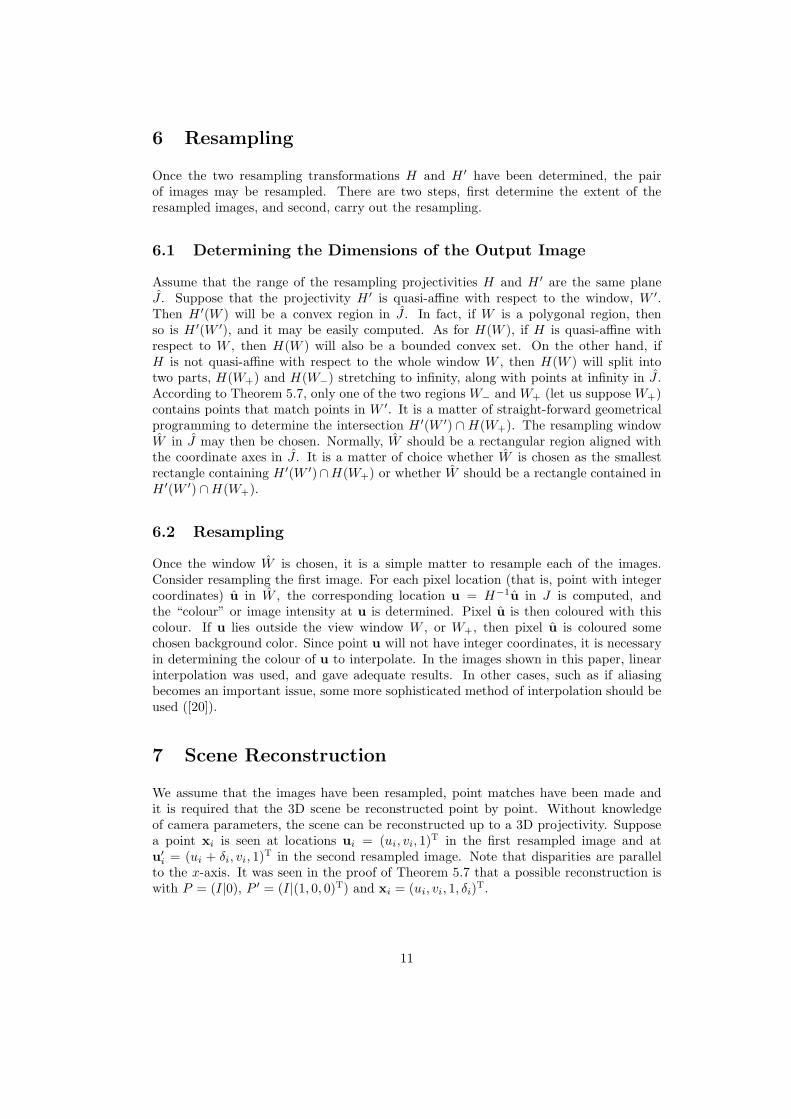
6 Resampling

Once the two resampling transformations H and H ′ have been determined, the pairof images may be resampled. There are two steps, first determine the extent of theresampled images, and second, carry out the resampling.

6.1 Determining the Dimensions of the Output Image

Assume that the range of the resampling projectivities H and H ′ are the same planeJ . Suppose that the projectivity H ′ is quasi-affine with respect to the window, W ′.Then H ′(W ) will be a convex region in J . In fact, if W is a polygonal region, thenso is H ′(W ′), and it may be easily computed. As for H(W ), if H is quasi-affine withrespect to W , then H(W ) will also be a bounded convex set. On the other hand, ifH is not quasi-affine with respect to the whole window W , then H(W ) will split intotwo parts, H(W+) and H(W−) stretching to infinity, along with points at infinity in J .According to Theorem 5.7, only one of the two regions W− and W+ (let us suppose W+)contains points that match points in W ′. It is a matter of straight-forward geometricalprogramming to determine the intersection H ′(W ′) ∩H(W+). The resampling windowW in J may then be chosen. Normally, W should be a rectangular region aligned withthe coordinate axes in J . It is a matter of choice whether W is chosen as the smallestrectangle containing H ′(W ′)∩H(W+) or whether W should be a rectangle contained inH ′(W ′) ∩H(W+).

6.2 Resampling

Once the window W is chosen, it is a simple matter to resample each of the images.Consider resampling the first image. For each pixel location (that is, point with integercoordinates) u in W , the corresponding location u = H−1u in J is computed, andthe “colour” or image intensity at u is determined. Pixel u is then coloured with thiscolour. If u lies outside the view window W , or W+, then pixel u is coloured somechosen background color. Since point u will not have integer coordinates, it is necessaryin determining the colour of u to interpolate. In the images shown in this paper, linearinterpolation was used, and gave adequate results. In other cases, such as if aliasingbecomes an important issue, some more sophisticated method of interpolation should beused ([20]).

7 Scene Reconstruction

We assume that the images have been resampled, point matches have been made andit is required that the 3D scene be reconstructed point by point. Without knowledgeof camera parameters, the scene can be reconstructed up to a 3D projectivity. Supposea point xi is seen at locations ui = (ui, vi, 1)T in the first resampled image and atu′i = (ui + δi, vi, 1)T in the second resampled image. Note that disparities are parallelto the x-axis. It was seen in the proof of Theorem 5.7 that a possible reconstruction iswith P = (I|0), P ′ = (I|(1, 0, 0)T) and xi = (ui, vi, 1, δi)T.

11

Looking closely at the form of the reconstructed point shows a curious effect of 3D pro-jective transformation. If the disparity δi is zero, then the point xi will be reconstructedas a point at infinity. As δi changes from negative to positive, the reconstructed pointwill flip from near infinity in one direction to near infinity in the other direction. In otherwords, the reconstructed scene will straddle the plane at infinity, and if interpreted in aEuclidean sense will contain points in diametrically opposite directions.

A different reconstruction of the 3D scene is possible which avoids points at infinity anddiametrically splitting the scene. In particular, if one of the images is translated by adistance α in the x direction, then a disparity of δi becomes a disparity of δi + α. Itfollows that the scene may be reconstructed with xi = (ui, vi, 1, δi + α)T are positive,that is δi +α > 0 for all i. Note that the eye makes this adjustment automatically whenviewing a stereo pair of images such as Figure 3, resulting in a sensible perception of thescene.

8 Algorithm Outline

The resampling algorithm will now be summarized. The input is a pair of images con-taining a common overlap region. The output is a pair of images resampled so thatthe epipolar lines in the two images are horizontal (parallel with the u axis), and suchthat corresponding points in the two images are as close to each other as possible. Anyremaining disparity between matching points will be along the the horizontal epipolarlines. A top-level outline of the image is as follows.

1. Identify a seed set of image-to-image matches ui ↔ u′i between the two images.Seven points at least are needed, though more are preferable. It is possible to findsuch matches by automatic means.

2. Compute the fundamental matrix F and find the epipoles p and p′ in the twoimages. The linear method of computation of F as the least-squares solution toequations (3) can be used, requiring eight point matches or more. For best results,the linear solution can be used as a basis for iteration to a least-squares solution.

3. Select a projective transformation H ′ that maps the epipole p′ to the point atinfinity, (1, 0, 0)T. The method of Section 3 gives good results.

4. Find the matching projective transformation H that minimizes the least-squaresdistance ∑

i

d(Hui, H ′u′i) . (10)

The method used is a linear method described in Section 4.

5. Resample the first image according to the projective transformation H and thesecond image according to the projective transformation H ′. A simple method isgiven in Section 6.

12

9 Examples

9.1 A pair of aerial images

The method was used to transform a pair of images of the Malibu area. Two imagestaken from widely different relatively oblique viewing angles are shown in Figure 2. A setof about 25 matched points were selected by hand and used to compute the fundamentalmatrix. The two 2D projective transformations necessary to transform them to matchedepipolar projections were computed and applied to the images. The resulting resampledimages are shown side-by-side in Figure 3 As may be discerned, any disparities betweenthe two images are parallel with the x-axis. By crossing the eyes it is possible to view thetwo images in stereo. The perceived scene looks a little strange, since it has undergonean apparent 3D projective transformation. However, the effect is not excessive.

9.2 A pair of images of an airfield

In the next example (see Figure 4), the the pair of images taken on different days arerectified to create a stereo pair. These two images may be merged to create a 3D im-pression. This example suggests that rectification may be used as an aid in detectingchanges in the two images, which become readily apparent when the images are viewedstereoscopically.

9.3 Satellite images

Although satellite images are not strictly speaking perspective images, they are suffi-ciently close to being perspective projections that the techniques described in this papermay be applied. To demonstrate this, the algorithm was applied to two satellite images,one Landsat image and one SPOT image. These two images have different resolutionsand different imaging geometries. In this case, a set of seed matches were found, thistime automatically, and the two images were resampled. (The method of finding seedmatches for differently oriented images is based on local resampling.) The results areshown in Figure 5 which shows the images after resampling.

9.4 Non-aerial images

The method may also be applied to images other than aerial images. Figure 6 showsa pair of images of some wooden block houses. Edges and vertices in these two imageswere extracted automatically and a small number of common vertices were matched byhand. The two images were then resampled according to the methods desribed here. Theresults are shown in Figure 7. In this case, because of the wide difference in viewpoint,and the three-dimensional shape of the objects, the two images even after resamplinglook quite different. However, it is the case that any point in the first image will nowmatch a point in the second image with the same y coordinate. Therefore, in order tofind further point matches between the images only a one-dimensional search is required.

13

10 Conclusion

This paper gives a firm mathematical basis as well as a rapid practical algorithm for therectification of stereo images taken from widely different viewpoints. The method givenavoids the necessity for camera calibration and provides significant gains in speed andease of point matching. In addition, it makes the computational of the scene geometryextremely simple. The time taken to resample the image is negligeable compared withother processing time. Because of the great simplicity of the projective transformation,the resampling of the images may be done extremely quickly. With carefully program-ming, it is possible to resample the images in about 20 seconds each for 1024 × 1024images on a Sparc station 1A.

References

[1] Nicholas Ayache and Charles Hansen, “Rectification of Images for Binocular andTrinocular Stereovision”, Proc. 9th International Conference on Pattern Recogni-tion, Rome, 1988, pp. 11–16.

[2] Nicholas Ayache and Francis Lustman, “Trinocular Stereo Vision for Robotics”,IEEE Transactions on PAMI, Vol 13, No. 1, January 1991, pp. 73–85.

[3] Patrick Courtney, Neil A. Thacker and Chris R. Brown, “A Hardware Architecturefor Image Rectification and Ground Plane Obstacle Avoidance”, Proc. 11th IAPR,ICPR 1992, pp. 23–26.

[4] Faugeras, O., “What can be seen in three dimensions with an uncalibrated stereorig?”, Proc. of ECCV-92, G. Sandini Ed., LNCS-Series Vol. 588, Springer- Verlag,1992, pp. 563 – 578.

[5] Faugeras, O. and Maybank, S., “Motion from Point Matches : Multiplicity of Solu-tions,” International Journal of Computer Vision, 4, (1990), 225–246.

[6] O. D. Faugeras, Q.-T. Luong and S. J. Maybank, “Camera Self-Calibration: The-ory and Experiments”, Proc. of ECCV-92, G. Sandini Ed., LNCS-Series Vol. 588,Springer- Verlag, 1992, pp. 321–334.

[7] R. Hartley, R. Gupta and T. Chang, “Stereo from Uncalibrated Cameras”, Proceed-ings Computer Vision and Pattern Recognition conference (CVPR-92), 1992.

[8] R. Hartley, “Estimation of Relative Camera Positions for Uncalibrated Cameras,”,Proc. of ECCV-92, G. Sandini Ed., LNCS-Series Vol. 588, Springer- Verlag, 1992,pp. 579 – 587.

[9] R. Hartley, “Cheirality Invariants”, Proc. Darpa Image Understanding Workshop,April, 1993, pp. 745–753

[10] H.C. Longuet-Higgins, “A computer algorithm for reconstructing a scene from twoprojections,” Nature, Vol. 293, 10 Sept. 1981.

[11] , “Manual of Photogrammetry, Fourth Edition”, Chester C. Slama, editor. AmericanSociety of Photogrammetry, Falls Church, Va, 1980.

14

[12] R. Mohr, F. Veillon, L. Quan, “Relative 3D Reconstruction Using Multiple Uncali-brated Images”, Proc. CVPR-93, pp 543-548.

[13] D. V. Papadimitriou and T. J. Dennis, “Epipolar Line Estimation and Rectificationfor Stereo Image Pairs”, IEEE Transactions on Image Processing, Vol 5, No. 4, April1996, pp. 672–676.

[14] William H. Press, Brian P. Flannery, Saul A. Teukolsky, William T. Vetterling,“Numerical Recipes in C”, Cambridge University Press, Cambridge, England, 1988

[15] Luc Robert, Michel Buffa and Martial Hebert, “Weakly-Calibrated Stereo Percep-tion for Rover Navigation”, Proc. 5th International Conference on Computer Vision,Cambridge Mass, 1995, pp. 46 –51.

[16] V. Rodin and A. Ayache, “Axial Stereovision : Modelization and Comparison Be-tween Two Calibration Methods”, Proc. ICIP-94, pp. 725 – 729.

[17] Fergal Shevlin, “Resampling of Scanned Imagery for Rectification and Registration”,Proc. ICIP-94, pp. 1007–1011.

[18] Rudolf Sturm, Das Problem der Projektivitat und seine Anwendung auf die Flachenzweiten Grades. Math. Ann., 1:533-574, 1869.

[19] Thierry Toutin and Yves Carbonneau, “MOS and SEASAT Image Geometric Cor-rections”, IEEE Transactions on Geoscience and Remote Sensing, Vol 30, No. 3,May 1992, pp. 603–609

[20] George Wolberg, “Digital Image Warping”, IEEE Computer Society Press, LosAlamitos, California, 1990.

15

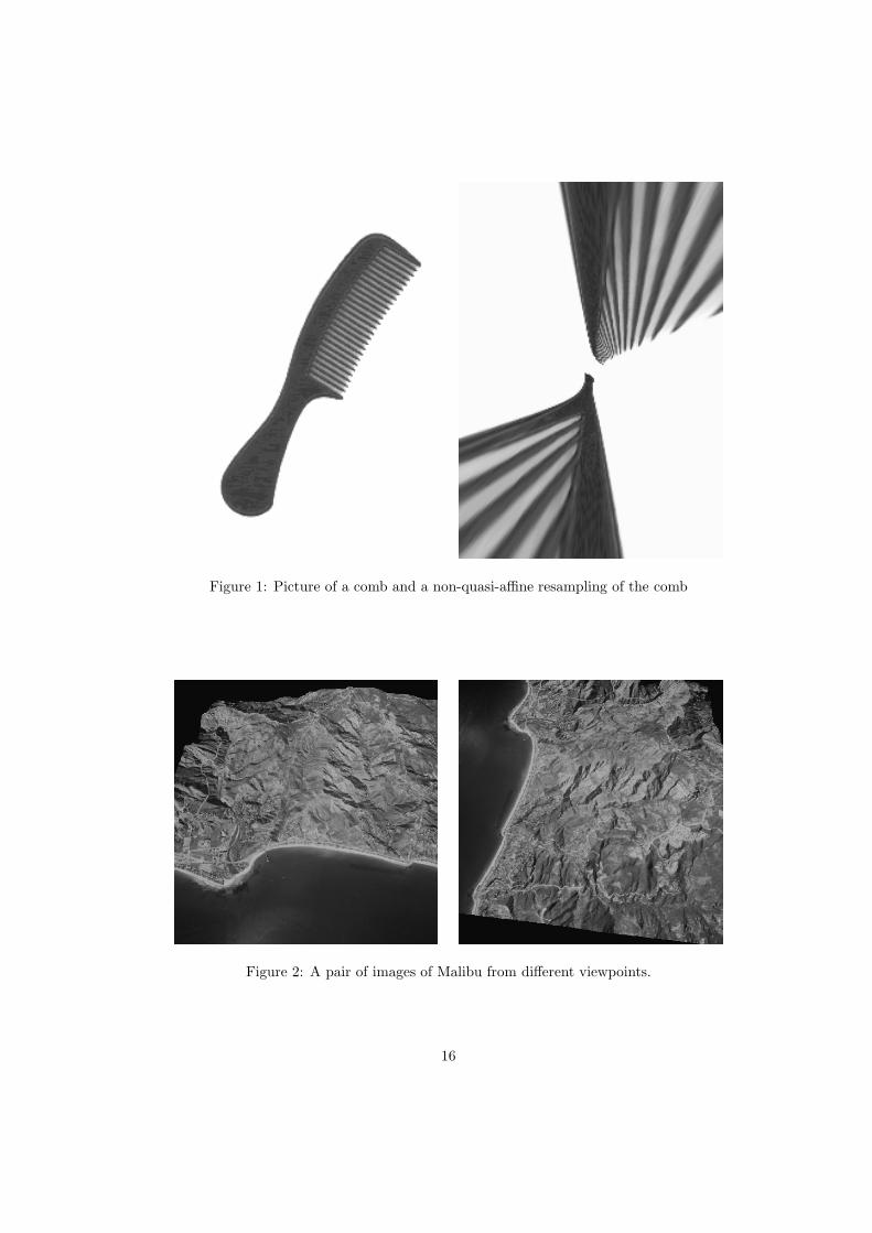
Figure 1: Picture of a comb and a non-quasi-affine resampling of the comb

Figure 2: A pair of images of Malibu from different viewpoints.

16

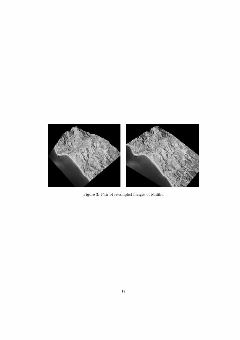
Figure 3: Pair of resampled images of Malibu

17

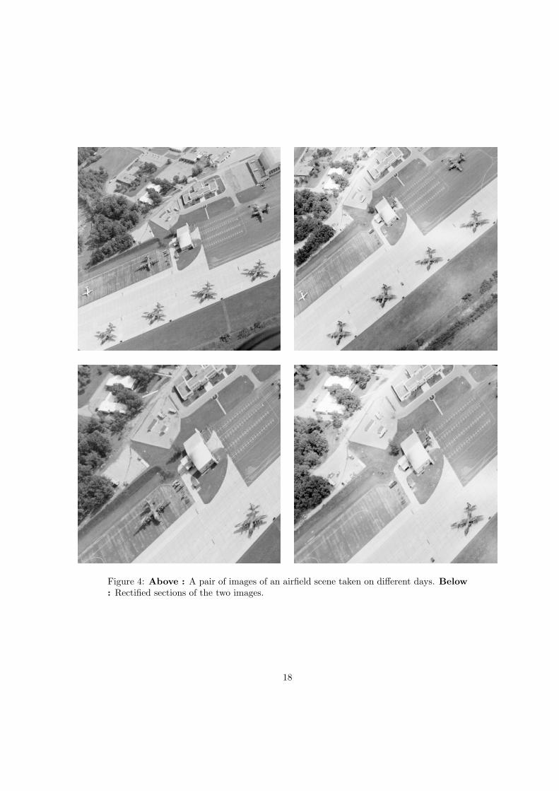
Figure 4: Above : A pair of images of an airfield scene taken on different days. Below: Rectified sections of the two images.

18

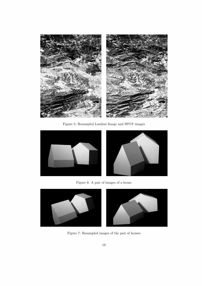
Figure 5: Resampled Landsat Image and SPOT images

Figure 6: A pair of images of a house

Figure 7: Resampled images of the pair of houses

19