Theory and Monte Carlo simulations for the stretching of flexible andsemiflexible single polymer chains under external fieldsFabio Manca, Stefano Giordano, Pier Luca Palla, Fabrizio Cleri, and Luciano Colombo Citation: J. Chem. Phys. 137, 244907 (2012); doi: 10.1063/1.4772656 View online: http://dx.doi.org/10.1063/1.4772656 View Table of Contents: http://jcp.aip.org/resource/1/JCPSA6/v137/i24 Published by the American Institute of Physics. Additional information on J. Chem. Phys.Journal Homepage: http://jcp.aip.org/ Journal Information: http://jcp.aip.org/about/about_the_journal Top downloads: http://jcp.aip.org/features/most_downloaded Information for Authors: http://jcp.aip.org/authors

THE JOURNAL OF CHEMICAL PHYSICS 137, 244907 (2012)

Theory and Monte Carlo simulations for the stretching of flexibleand semiflexible single polymer chains under external fields

Fabio Manca,1 Stefano Giordano,2,3,a) Pier Luca Palla,2,4 Fabrizio Cleri,2,4

and Luciano Colombo1

1Department of Physics, University of Cagliari, 09042 Monserrato, Italy2Institute of Electronics, Microelectronics and Nanotechnology (UMR CNRS 8520),59652 Villeneuve d’Ascq, France3International Associated Laboratory LEMAC/LICS, ECLille, 59652 Villeneuve d’Ascq, France4University of Lille I, 59652 Villeneuve d’Ascq, France

(Received 23 October 2012; accepted 5 December 2012; published online 28 December 2012)

Recent developments of microscopic mechanical experiments allow the manipulation of individ-ual polymer molecules in two main ways: uniform stretching by external forces and non-uniformstretching by external fields. Many results can be thereby obtained for specific kinds of polymers andspecific geometries. In this work, we describe the non-uniform stretching of a single, non-branchedpolymer molecule by an external field (e.g., fluid in uniform motion, or uniform electric field) bya universal physical framework, which leads to general conclusions on different types of polymers.We derive analytical results both for the freely-jointed chain and the worm-like chain models basedon classical statistical mechanics. Moreover, we provide a Monte Carlo numerical analysis of themechanical properties of flexible and semiflexible polymers anchored at one end. The simulationsconfirm the analytical achievements, and moreover allow to study the situations where the theorycannot provide explicit and useful results. In all cases, we evaluate the average conformation of thepolymer and its fluctuation statistics as a function of the chain length, bending rigidity, and fieldstrength. © 2012 American Institute of Physics. [http://dx.doi.org/10.1063/1.4772656]

I. INTRODUCTION

Modern methods for stretching single molecules providea valuable insight about the response of polymers to exter-nal forces. The interest on single molecules loading encour-aged new research and technological developments on relatedmechanical experiments. Typically, mechanical methods al-low the manipulation of a polymer molecule in two ways:the stretching of the chain by the direct action of an exter-nal force or by the application of an external field. If we con-sider homogeneous polymers (with all monomers describedby the same effective elastic stiffness), then we obtain a uni-form strain with the external force and a non-uniform strainwith the applied field.

To exert an external force on a polymer fixed at one end,laser optical tweezers (LOTs),1 magnetic tweezers (MTs),2 oratomic force microscope (AFM)3 can be used. Many exper-iments have been performed over a wide class of polymerswith biological relevance, such as the nucleic acids (DNA,RNA),4 allowing the stretching of the entire molecule andproviding the reading and the mapping of genetic informa-tion along the chain.5, 6 Furthermore, it has been possible todescribe the elastic behavior of single polymers consistingof domains, which may exhibit transitions between differ-ent stable states.7, 8 Other investigations performed on double-stranded DNA determined the extension of the polymer as afunction of the applied force,9 providing results in very good

a)Electronic mail: stefano.giordano@iemn.univ-lille1.fr.

agreement with the worm-like chain (WLC) model10–12 andthe freely-jointed chain (FJC) model.12, 13

Alternatively, it is possible to manipulate singlemolecules by an external field. In this case, the external fieldacts on the molecules from a distance or, in other words, with-out a defined contact point for applying the traction. A non-uniform stretching performed by an external field can be in-duced either via a hydrodynamic (or electrohydrodynamic)flow field,14–16 or via an electric (or magnetic) field.17–19

One experimental advantage of using flow fields is that theliquid surrounding the tethered molecule can be easily re-placed; this is indeed an important feature for many single-molecules studies of enzymes, which require varying bufferconditions.20 The flow field technique was extensively ap-plied in single-molecule study of DNA elasticity10 as well asto characterize the rheological properties of individual DNAmolecules.21–23 The use of an electric field has been adoptedfor driving the alignment of DNA on a solid surface for appli-cations such as gene mapping and restriction analysis.17 Fi-nally, magnetic fields have been used to apply torsional stressto individual DNA molecules.18, 19

A key issue in polymer theory concerns the determina-tion of the physical properties of chains starting from theknowledge of the actual chemical architecture and environ-mental conditions.24, 25 Consequently, the response of singlepolymers can be used to predict and analyze the behaviorof most complex systems such as networks and rubber-likematerials.26, 27 In order to realize the first step of this mat-ter, a number of mathematical models have been developedfor describing the mechanical response of polymers in differ-

0021-9606/2012/137(24)/244907/12/$30.00 © 2012 American Institute of Physics137, 244907-1

244907-2 Manca et al. J. Chem. Phys. 137, 244907 (2012)

ent chemical and loading conditions.28–30 The standard ap-proaches for studying polymer elasticity are based on theFJC (flexible) and WLC (semiflexible) models. A techniquedescribing the crossover between these two classes of mod-els has been recently introduced.31 It has been shown thatthe alternative between these two regimes depends on thechain bending rigidity and the magnitude of the applied force.Moreover, we remark that models for semiflexible polymerchains can be realized both with continuum and discretestructures. The comparison between these two approachesand their applicability has been largely investigated.32 A re-fined technique that has led to important results for the WLCmodel is based on the path integral formalism (functionalintegration).33–37 In fact, it has been proved that the calcula-tion of the partition function for a continuous polymer chainexactly corresponds to a Feynmann path integral, as intro-duced in quantum mechanics.38 All previous methodologieshave been typically developed for analysing homopolymers,but can be also generalised to heteropolymers.39, 40

In order to understand the response of polymers to ex-ternal fields, FJC and WLC schemes have been applied asdescribed below. Some studies show that in a weak exter-nal field, the persistence length along the field direction isincreased, while it is decreased in the perpendicular direc-tion; moreover, as the external field becomes stronger, the ef-fective persistence length grows exponentially with the fieldstrength.41–43 The behavior of a Gaussian chain in an elonga-tional flow has been studied through the dumbbell model.44

Other investigations under a constant velocity flow haveshown that a flexible polymer displays three types of confor-mations: unperturbed at low velocity; “trumpet” shaped whenpartially stretched; “stem and flowers” shaped, with a com-pletely stretched portion (the stem), and a series of blobs (theflowers), at larger loading.45–47 Polymer models have beenstudied in elongational flows to analyze the coil stretchingand chain retraction as a function of polymer and flow pa-rameters, finding good agreement with experimental data.48, 49

Conformational properties of semiflexible polymer chains inuniform force field were also studied for two-dimensionalmodels.50 Some important results have been obtained for thedynamic behavior of polymers containing positive and nega-tive charges in the presence of external electrical fields.51–54

In spite of all these relevant efforts, it is yet a challenge tobase on the same unified theoretical framework all aspects ofpolymer mechanics in an external field.

Building on our previous studies,12 in this paper we studythe conformational and mechanical properties of flexible andsemiflexible non-branched polymer model chains tethered atone end and immersed in an external force field. This situationis useful to describe almost two physical conditions of inter-est: a polymer chain immersed in a fluid in a uniform motion(our model is valid only when the action of the fluid motioncan be described by a distribution of given forces applied toall monomers) and an arbitrarily charged chain inserted in auniform electric field.

Our theoretical approach is twofold, since we adopt bothanalytical (statistical mechanics27, 55) and numerical tech-niques (Monte Carlo simulations56, 57). While the analyticalapproach is useful to obtain the explicit partition function and

the force-extension curve in some specific cases, Monte Carlosimulations are crucial to check the theoretical results and tostudy more generic situations, inaccessible to analytical treat-ments. In particular, while we develop our exact mathemati-cal analysis starting from the more tractable FJC model, wetake into consideration some classical approximations to ex-tend our theoretical study also to the WLC model. Finally,several comparisons have been drawn and more complex ge-ometries have been analyzed by taking full profit from the MCsimulations.

The structure of the paper is the following. In Sec. II, weintroduce the mathematical formalism adopted and derive ageneric form of the partition function in Rd for a generalizedFJC model, where the extensibility of the bonds is taken intoaccount. In Sec. III, we find the two specific forms of the par-tition function for the 2D- and the 3D-case for the pure FJCpolymer with non-extensible bonds. Moreover, we obtain inboth cases: the variance and the covariance among the posi-tions of the monomers. In Sec. IV, we present the generaliza-tion of previous results to the semiflexible WLC model. Wepresent two closed-forms approximations for the 2D- and the3D-case with the presence of an external field, which repre-sent a generalization of the classical Marko-Siggia results.11

Monte Carlo simulations are performed and comparisons withtheoretical results are found to be in perfect agreement. InSec. V, we analyze the behavior of a chain in an external fieldto which also an external force is applied at the end of thechain. The case with the force not aligned with the field is par-ticularly interesting and shows the power of the MC method.Finally, in Sec. VI, some conclusions are drawn.

II. GENERAL THEORETICAL FRAMEWORK

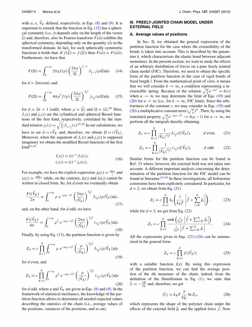
As previously discussed, the polymer models most usedin literature are the FJC and the WLC. As argued in Ref. 58,for weak tension and weak external field, it is acceptable tomodel the polymer as a FJC model. This model breaks downonly when the curvature of the conformation is very large be-cause it ignores the consequent great bending energy. Sincewe will look upon this problem in the end of this work, wenow give way to the case of a FJC. In particular, we considera FJC with two additional hypothesis. First, we consider thepossible extensibility of the bonds of the chain through a stan-dard quadratic potential characterized by a given equilibriumlength: such an extension mimics the possible stretching ofthe chemical bond between two adjacent monomers. If nec-essary, the extensibility of the bonds, here described by linearsprings, can be easily extended to more complex, nonlinearsprings.59 Moreover, we take into account a series of arbi-trary forces applied to each monomer: these actions mimicthe effects of an external physical field applied to the system.In addition, we contemplate the presence of an arbitrary forceapplied to the terminal monomer of the chain. All calculationswill be performed in Rd and we will specialize the results bothin the 2D-case and in the 3D-case when needed. The idea isto write the complete form of the Hamiltonian of the systemand to build up the corresponding statistical mechanics.12 Thestarting point is therefore the calculation of the classical par-tition function. In fact, when this quantity is determined, it is

244907-3 Manca et al. J. Chem. Phys. 137, 244907 (2012)

r0

r1 r2

rK

rN−1

k

k

k

k

FIXED

f

rN

gN

gN−1

gK

g2

g1

FIG. 1. A polymer chain in an external field. The first monomer is clamped atposition �r0 while the others are free to fluctuate. Each monomer is subjectedto an external force �gK (different in strength and direction for any K): allthese forces mimic an external field. Another external force, playing the roleof a main pulling load, �f , is applied to the last monomer at the position �rN .

possible to obtain the force-extension curve (the equation ofstate) through simple derivations.

Let us consider a non-branched linear polymer with Nmonomers (see Fig. 1) at positions defined by �r1, . . . , �rN ∈�d (for considering d = 2 or d = 3 according to the spe-cific problem of interest). To each monomer, a given exter-nal force is applied and named �g1, . . . , �gN . Another externalforce, playing the role of main pulling load, �f , is appliedto the last monomer at the position �rN . While the chain isclamped at position �r0, the monomers are free to fluctuate.The Hamiltonian of the system is therefore given by

H =N∑

i=1

�pi · �pi

2m+ 1

2k

N∑K=1

(|�rK − �rK−1| − l)2

−N∑

K=1

�gK · �rK − �f · �rN , (1)

where �pi are the linear momenta, m the mass of themonomers, k the spring constant of the inter-monomer inter-action, and l the equilibrium length of the monomer-monomerbond. We search for the partition function of the system de-fined as

Zd = c

∫�d

. . .

∫�d︸ ︷︷ ︸

2N−times

exp

(− H

kBT

)d�r1 . . . d�rNd �p1 . . . d �pN,

(2)

where c is a multiplicative constant, which takes into accountthe number of microstates. As well known, the kinetic partcan be straightforwardly integrated and it yields a furthernon-influencing multiplicative constant; then we can writethe partition function as an integral over the positional spaceonly. This integral can be easily handled through the standardchange of variable ⎧⎪⎪⎪⎪⎨

⎪⎪⎪⎪⎩

�ξ1 = �r1 − �r0

�ξ2 = �r2 − �r1...

�ξN = �rN − �rN−1

(3)

having the Jacobian determinant J =∣∣∣ ∂(�r1...�rN )∂(�ξ1...�ξN )

∣∣∣ = 1. We con-

sider the terminal �r0 of the chain fixed in the origin of axes, i.e.�r0 = �0. So, we cast the positions �ri in terms of the variables�ξJ as follows:⎧⎪⎪⎪⎪⎨

⎪⎪⎪⎪⎩

�r1 = �ξ1 + �r0 = �ξ1

�r2 = �ξ2 + �r1 = �ξ2 + �ξ1...

�rN = �ξN + �ξN−1 + . . . + �ξ1.

(4)

By setting the general solution as �ri = ∑iK=1

�ξK , the partitionfunction becomes

Zd = c

∫�d

. . .

∫�d︸ ︷︷ ︸

N−times

exp

[− k

2kBT

N∑K=1

(|�ξK | − l)2

]

× exp

[1

kBT

N∑K=1

�gK ·K∑

J=1

�ξJ

]

× exp

[1

kBT�f ·

N∑K=1

�ξK

]d�ξ1 . . . d�ξN . (5)

Inverting the two summation symbols

N∑K=1

�gK ·K∑

J=1

�ξJ =N∑

K=1

�ξK ·N∑

i=K

�gi (6)

we obtain

Zd = c

N∏K=1

∫�d

e−a(|�ξ |−l)2e

�VK ·�ξ d�ξ, (7)

where

a = k

2kBT> 0, (8)

�VK = 1

kBT

(�f +

N∑i=K

�gi

). (9)

There exists a deep conceptual connection between the lastintegral for the partition function and the theory of the d-dimensional Fourier transforms. The Fourier integral of anarbitrary function f (�ξ ) is defined as

F ( �ω) =∫

�d

f (�ξ )e−i �ω·�ξ d�ξ (10)

with inverse transform given by

f (�ξ ) = 1

(2π )d

∫�d

F ( �ω)ei �ω·�ξ d �ω. (11)

If we consider

f (�ξ ) = e−a(|�ξ |−l)2, (12)

it is easy to realize that the integral in Eq. (7) is the Fouriertransform of f (�ξ ) calculated for �ω = i �VK , i.e.,

Zd = c

N∏K=1

F (i �VK ) (13)

244907-4 Manca et al. J. Chem. Phys. 137, 244907 (2012)

with a, e, �VK defined, respectively, in Eqs. (8) and (9). It isimportant to remark that the function in Eq. (12) has a spheri-cal symmetry (i.e., it depends only on the length of the vector�ξ ) and, therefore, also its Fourier transform F ( �ω) exhibits thespherical symmetry, depending only on the quantity | �ω| in thetransformed domain. In fact, for such spherically-symmetricfunctions it holds that: if f (�ξ ) = f (|�ξ |) then F ( �ω) = F (| �ω|).Furthermore, we have that

F (�) =∫ +∞

02πρf (ρ)

(2πρ

�

) d2 −1

J d2 −1(ρ�)dρ (14)

for d = 2n(even), and

F (�) =∫ +∞

04πρ2f (ρ)

(2πρ

�

) d−32

j d−32

(ρ�)dρ (15)

for d = 2n + 1 (odd), where ρ = |�ξ | and � = |�ω|.60 Here,Jν(z) and jν(z) are the cylindrical and spherical Bessel func-tions of the first kind, respectively, correlated by the stan-

dard relation jν(z) =√

π2z

Jν+ 12(z).61, 62 In our calculations, we

have to set �ω = i �VK and, therefore, we obtain � = i| �VK |.Moreover, when the argument of Jν(z) and jν(z) is supposedimaginary we obtain the modified Bessel functions of the firstkind61, 62

Iν(z) = (i)−νJν(iz),

iν(z) = (i)−νjν(iz).(16)

For example, we have the explicit expression j0(z) = sin zz

andi0(z) = sinh z

zwhile, on the contrary, I0(z) and J0(z) cannot be

written in closed form. So, for d even we eventually obtain

F (i �VK )

2π=∫ +∞

0ρ e−a(ρ−l)2

(2πρ

| �VK |

) d−22

I d−22

(ρ| �VK |)dρ,

(17)and, on the other hand, for d odd, we have

F (i �VK )

4π=∫ +∞

0ρ2 e−a(ρ−l)2

(2πρ

| �VK |

) d−32

i d−32

(ρ| �VK |)dρ.

(18)Finally, by using Eq. (13), the partition function is given by

Zd = c

N∏K=1

∫ +∞

0ρ e−a(ρ−l)2

(ρ

| �VK |

) d−22

I d−22

(ρ| �VK |)dρ(19)

for d even, and

Zd = c

N∏K=1

∫ +∞

0ρ2 e−a(ρ−l)2

(ρ

| �VK |

) d−32

i d−32

(ρ| �VK |)dρ(20)

for d odd, where a and �VK are given in Eqs. (8) and (9). In theframework of statistical mechanics, the knowledge of the par-tition function allows to determine all needed expected valuesdescribing the statistics of the chain (i.e., average values ofthe positions, variances of the positions, and so on).

III. FREELY-JOINTED CHAIN MODEL UNDEREXTERNAL FIELD

A. Average values of positions

In Sec. II, we obtained the general expression of thepartition function for the case where the extensibility of thebonds is taken into account. This is described by the param-eter k, which characterizes the elastic bond between adjacentmonomers. In the present section, we want to study the effectsof an arbitrary distribution of forces on a pure freely jointedchain model (FJC). Therefore, we need to obtain the specificform of the partition function in the case of rigid bonds offixed length l. From the mathematical point of view, it meansthat we will consider k → ∞, a condition representing a in-extensible spring. Because of the relation

√απe−αx2 = δ(x)

when α → ∞ we may determine the limit of Eqs. (19) and(20) for a → ∞ (i.e., for k → ∞, FJC limit). Since the arbi-trariness of the constant c, we may consider in Eqs. (19) and(20) a multiplicative constant term (

√aπ

)N . Then, by using the

translated property√

aπe−a(ρ−l)2 → δ(ρ − l) for a → ∞, we

perform all the integrals thereby obtaining

Zd = c

N∏K=1

1

| �VK | d−22

I d−22

(l| �VK |), d even, (21)

Zd = c

N∏K=1

1

| �VK | d−32

i d−32

(l| �VK |), d odd. (22)

Similar forms for the partition function can be found inRef. 33 where, however, the external field was not taken intoaccount. A different important analysis concerning the deter-mination of the partition function for the FJC model can befound in literature.63–65 In these investigations, all holonomicconstraints have been explicitely considered. In particular, ford = 2, we obtain from Eq. (21)

Z2 = c

N∏K=1

I0

(l

kBT

∣∣∣∣∣ �f +N∑

i=K

�gi

∣∣∣∣∣)

, (23)

while for d = 3, we get from Eq. (22)

Z3 = c

N∏K=1

sinh(

lkBT

∣∣∣ �f +∑Ni=K �gi

∣∣∣)l

kBT

∣∣∣ �f +∑Ni=K �gi

∣∣∣ . (24)

All the expressions given in Eqs. (21)–(24) can be summa-rized in the general form

Zd = c

N∏K=1

f (| �VK |) (25)

with a suitable function f(x). By using this expressionof the partition function, we can find the average posi-tion of the ith monomer of the chain; indeed, from thedefinition of the Hamiltonian in Eq. (1), we state that�ri = − ∂H

∂ �giand, therefore, we get

〈�ri〉 = kBT∂

∂ �gi

ln Zd, (26)

which represents the shape of the polymer chain under theeffects of the external field �gi and the applied force �f . Now

244907-5 Manca et al. J. Chem. Phys. 137, 244907 (2012)

we can substitute Eq. (25) into Eq. (26), obtaining

〈�ri〉 =i∑

K=1

�VK

| �VK |

[1

f (x)

∂f (x)

∂x

]x=| �VK |

. (27)

In 2D, we have f(x) = I0(lx) and therefore we obtain

〈�ri〉 = l

i∑K=1

I1

(l

kBT

∣∣∣ �f +∑NJ=K �gJ

∣∣∣)I0

(l

kBT

∣∣∣ �f +∑NJ=K �gJ

∣∣∣)�f +∑N

J=K �gJ∣∣∣ �f +∑NJ=K �gJ

∣∣∣ .(28)

For such a 2D case, by applying Eq. (28), the average val-ues of the longitudinal component of the positions have beencalculated and are plotted in Fig. 2 as a function of the chainlength N and the field strength g. We have considered only theaction of an external uniform field with �gJ = �g and amplitudeg.

Although this case lends itself to a full analytical solu-tion, numerical simulations were also performed by using aconventional implementation of the Metropolis version of theMonte Carlo algorithm.56 The initial state of the chain is de-fined by a set of randomly chosen positions. The displace-ment extent of each step governs the efficiency of the con-figurational space sampling. Therefore, we analyzed severalruns in order to optimize its value.66, 67 The perfect agreementbetween the theory and the MC simulations provides a strictcheck of the numerical procedure, to be used in the foregoing.

0 0.5 10

10

20

30

40

50

r i,l

/l

i/N

N

2D−FJC

0 0.5 10

5

10

15

20

25

r i,l

/l

i/N

g2D−FJC

FIG. 2. Average values of the longitudinal component of the positions in-duced by the external field for the 2D FJC case. The red solid lines correspondto the analytical results Eqs. (28) and (32), MC results are superimposed inblack circles. Top panel: each curve corresponds to different chain lengths N= 10, 20, 30, 40, 50 for a fixed value gl/(kBT) = 1 (e.g., corresponding tol = 1 nm, g = 4 pN at T = 293 K). Bottom panel: each curve correspondsto the different values gl/(kBT) = 0.1, 0.25, 0.5, 1, 2, 10 for a fixed chainlength N = 20.

On the other hand, in 3D we have f (x) = sinh(lx)lx

, leadingto

〈�ri〉 = l

i∑K=1

L(

l

kBT

∣∣∣∣∣ �f +N∑

J=K

�gJ

∣∣∣∣∣) �f +∑N

J=K �gJ∣∣∣ �f +∑NJ=K �gJ

∣∣∣ ,(29)

where L(x) = coth x − 1x

is the Langevin function. By usingEq. (29), as before, it is possible to plot the average values ofthe longitudinal component of the positions for the 3D case(Fig. 3). Also in this case, we adopted a uniform field g andthe good agreement with the MC simulations is evident.

As particular case, if there is only the force �f appliedto the system, we obtain the standard scalar force-extensioncurves linking r = |〈�rN 〉| with f = | �f |. In 2D, we have

r

lN=

I1

(lf

kBT

)I0

(lf

kBT

) (30)

in agreement with recent results,68 while in 3D we obtain

r

lN= L

(lf

kBT

), (31)

which is a classical result.12, 28 The simple results in Eqs. (30)and (31) have been used to obtain the limiting behaviors underlow (f → 0) and high (f → ∞) values of the applied force, asshown in Table I.

Building on such first results, we now focus on some par-ticular interesting approximations. More specifically, it canbe interesting to find approximate results for the case of ahomogeneous field and no end-force, �f = 0 and �gJ = �g forany J. In this case, we search for the scalar relation between

0 0.5 10

10

20

30

40

50

r i,l

/l

i/N

N

3D−FJC

0 0.5 10

5

10

15

20

r i,l

/l

i/N

g3D−FJC

FIG. 3. Average values of the longitudinal component of the positions in-duced by the external field for the 3D FJC case. The red solid lines correspondto the analytical results Eqs. (29) and (33), MC results are superimposed inblack circles. Top panel: each curve corresponds to different chain lengths N= 10, 20, 30, 40, 50 for a fixed value gl/(kBT) = 1. Bottom panel: each curvecorresponds to the different values gl/(kBT) = 0.1, 0.25, 0.5, 1, 2, 10 for afixed chain length N = 20.

244907-6 Manca et al. J. Chem. Phys. 137, 244907 (2012)

TABLE I. Asymptotic forms of the force-extension curves for all cases de-scribed in the paper: FJC and WLC models in 2D and 3D geometry withforce applied f or field applied g.

Asymptotic form Asymptotic formof r

lNfor f, g → 0 of r

lNfor f, g → ∞(

x = lfkBT

or lgkBT

) (x = lf

kBTor lg

kBT

)Polymer chain︸ ︷︷ ︸Equation

FJC (2D) f︸ ︷︷ ︸Eq. (30)

1

2x 1 − 1

2x

FJC (3D) f︸ ︷︷ ︸Eq. (31)

1

3x 1 − 1

x

FJC (2D) g︸ ︷︷ ︸Eq. (32)

1

2

(1 + N

2

)x 1 − log(N + 1)

2N

1

x

FJC (3D) g︸ ︷︷ ︸Eq. (33)

1

3

(1 + N

2

)x 1 − log(N + 1)

N

1

x

WLC (2D) f︸ ︷︷ ︸Eq. (44)

Lp

lx 1 − 1

4

1√Lp

lx

WLC (3D) f︸ ︷︷ ︸Eq. (47)

2

3

Lp

lx 1 − 1

2

1√Lp

lx

WLC (2D) g︸ ︷︷ ︸Eq. (46)

Lp

l

(1 + N

2

)x 1 − 1√

Lp

lx

√N + 1 − 1

2N

WLC (3D) g︸ ︷︷ ︸Eq. (48)

2

3

Lp

l

(1 + N

2

)x 1 − 1√

Lp

lx

√N + 1 − 1

N

r = |〈�rN 〉| and g = |�g|. In the 2D case, from Eq. (28), we have

r

lN= 1

N

N∑k=1

I1(

lg

kBT(N − k + 1)

)I0(

lg

kBT(N − k + 1)

) , 1

N

∫ N

0

I1(

lg

kBT(N − x + 1)

)I0(

lg

kBT(N − x + 1)

)dx,

= 1

N

1lg

kBT

logI0(

lg

kBT(N + 1)

)I0(

lg

kBT

) . (32)

On the other hand, for the 3D case we obtain

r

lN= 1

N

N∑K=1

L(

l

kBT(N − k + 1)

),

1

N

∫ N

0L(

l

kBT(N − x + 1)

)dx,

= 1

N

1lg

kBT

loge2 lg

kB T(N+1) − 1

(N + 1)(e2 lg

kB T − 1) − 1. (33)

We have usefully exploited the fact that, for large N, the sumscan be approximately substituted with the corresponding in-tegrals, which are easier to be handled. The closed-form ex-pressions given in Eqs. (32) and (33) are very useful to ob-tain the limiting behaviors of the polymer under low (g → 0)and high (g → ∞) values of the applied field, as shown inTable I. Moreover, we verified the validity of Eqs. (32) and

(33) through a series of comparisons with MC results (seeFig. 6 in Sec. IV for details).

B. Covariances and variances of positions

In this section, we search for the covariance among thepositions of the monomers. It is important to evaluate sucha quantity in order to estimate the variance of a given posi-tion (measuring the width of the probability density around itsaverage value) and the correlation among different monomerpositions (measuring the persistence of some geometrical fea-tures along the chain). In order to do this, we identify the αthcomponent of the ith monomer as riα . The covariance of thegeneric monomer simply defined as (it represent the expecta-tion value of the second order)

Cov(riα, rJβ ) = 〈(riα − 〈riα〉)(rJβ − 〈rJβ〉)〉,= 〈riαrJβ〉 − 〈riα〉〈rJβ〉. (34)

Taking the derivative of the partition function with respect tothe α and the β components of the force vectors �gi and �gJ , wecan solve the problem as follows. We consider the standardexpression for the partition function and we can elaborate thefollowing expression:

〈riαrJβ〉 = (kBT )2

(∂ ln Zd

∂giα

∂ ln Zd

∂gJβ

+ ∂2 ln Zd

∂giα∂gJβ

), (35)

or, equivalently, by introducing Eq. (26)

〈riαrJβ〉 = 〈riα〉〈rJβ〉 + kBT∂

∂gJβ

〈riα〉 , (36)

but we can simply determine that

∂

∂gJβ

〈riα〉 = ∂

∂gJβ

i∑K=1

�VK · �eα

| �VK |

[1

f (x)

∂f (x)

∂x

]x=| �VK |

, (37)

where we have defined the unit vector �eα as the basis of theorthonormal reference frame. Being

�VK · �eα = 1

kBT

(fα +

N∑i=K

giα

)(38)

and

∂| �VK |∂gJβ

= 1

kBT

�VK · �eβ

|VK |N∑

q=K

δJq (39)

after long but straightforward calculations, we obtain

kBT∂

∂gJβ

〈riα〉 =min{i,J }∑

K=1

1

| �VK|f (| �VK |)

×{δαβf ′(| �VK|) +f ′′(| �VK |)VKαVKβ

| �VK |

−VKαf ′(| �VK|) VKβ

| �VK|2 −VKα

f ′(| �VK|)2

f (| �VK |)VKβ

| �VK |

}.

(40)

244907-7 Manca et al. J. Chem. Phys. 137, 244907 (2012)

Ordering the terms, we finally obtain the important result

Cov(riα, rJβ ) =min{i,J }∑

K=1

δαβ

| �VK |f ′(| �VK |)f (| �VK |)

+min{i,J }∑

K=1

VKαVKβ

| �VK |2f (| �VK |)

×{

f ′′(| �VK |) − f ′(| �VK |)| �VK | − f ′(| �VK |)2

f (| �VK |)

}.

(41)

It represents the final form of the covariance betweentwo different components of the positions of two differentmonomers.

If we look at the variance of a single component of asingle position (i = J, α = β), we have the simpler result

σ 2iα =

i∑K=1

f ′(| �VK |)| �VK |f (| �VK |) +

i∑K=1

V 2Kα

| �VK |2f (| �VK |)

×{

f ′′(| �VK |) − f ′(| �VK |)| �VK | − f ′(| �VK |)2

f (| �VK |)

}. (42)

In order to use the previous expressions, we have tospecify the function f and its derivatives for the two-dimensional and the three-dimensional case. In the 2D case,we have f(x) = I0(lx), f ′(x) = lI1(lx), and f ′′(x) = l2

2 [I0(lx)+ I2(lx)]. On the other hand, for the 3D case, we havef (x) = sinh(lx)

lx, f ′(x)/f (x) = lL(lx), and f ′′(x)/f (x) = l2 −

2lL(lx)/x. This completes the determination of the covari-ance.

We report in Figs. 4 and 5 the longitudinal and transversalcomponent of the variance as a function of the chain lengthand the field strength for the 3D case (with f = 0). The 2Dcase is very similar and it has not been reported here for sakeof brevity. We can observe some interesting trends: the lon-gitudinal variance of the position is a decreasing function ofthe number of polymers N while the transversal one is a in-creasing function (with a fixed amplitude of the external fieldg). Moreover, both variances are rapidly increasing along thechain, assuming the largest value in the last free monomer,which is more subject to strong fluctuations. It interestingto observe that the variance (both longitudinal and transver-sal components) is a linear function of the position i alongthe chain (it linearly intensifies along the chain itself) witha simple force f applied at the free end: conversely, with auniform field g, the distribution of forces generates a stronglynon-linear intensification of the variances moving towards thefree end-terminal. So, from the point of view of the variances,the application of a field or the application of a single forcegenerates completely different responses. In Fig. 5, we canalso observe that the variances are decreasing functions of thestrength of the field (both for the longitudinal and transversalcomponents); in fact, the intensity of the fields tends to reducethe fluctuations of the chain, increasing, at the same time, thetension within the bonds.

These trends are in qualitative agreement with results re-ported in Refs. 45–47. In fact, the behavior of the variances

0 0.5 10

0.2

0.4

0.6

0.8

1

σ2 i,

l/l2

i/N

N

3D−FJC

0 0.5 10

1

2

3

4

σ2 i,

t/l

2

i/N

N

3D−FJC

FIG. 4. Longitudinal (top panel) and transversal (bottom panel) componentof the variance of positions for the 3D FJC case. The red solid lines corre-spond to the analytical result Eq. (42), MC results are superimposed in blackcircles. Each curve corresponds to different chain lengths N = 10, 20, 30, 40,50 for a fixed value of the external field defined by gl/(kBT) = 1.

reflects the fluctuations of the chain shape. As already dis-cussed, the polymer assumes different shapes for different ex-ternal field amplitudes. For moderate field, the trumpet regimewas observed, while for larger values of the field, the stem andflower shape was predicted.

0 0.5 10

2

4

6

8

σ2 i,

l/l2

i/N

g

3D−FJC

0 0.5 10

2

4

6

8

σ2 i,

t/l

2

i/N

g

3D−FJC

FIG. 5. Longitudinal (top panel) and transversal (bottom panel) componentof the variance of positions for the 3D FJC case. The red solid lines corre-spond to the analytical result Eq. (42), MC results are superimposed in blackcircles. Each curve corresponds to different values of the external field am-plitude defined by gl/(kBT) = 0.1, 0.25, 0.5, 1, 2, 10 for a fixed chain lengthN = 20.

244907-8 Manca et al. J. Chem. Phys. 137, 244907 (2012)

IV. WORM-LIKE CHAIN MODEL UNDEREXTERNAL FIELD

In Secs. II and III, we treated systems described by theFJC model, characterized by the complete flexibility of thechain and, therefore, by the absence of any bending contri-bution to the total energy. Nevertheless, in many polymerchains, especially of biological origin, the specific flexibility(described by the so-called persistence length69) has a rele-vant role in several bio-mechanical processes. In order to takeinto consideration these important features, with relevant ap-plications to bio-molecules and bio-structures, in this sectionwe introduce the semiflexible polymer chain characterized bya given bending energy added to the previous Hamiltonian

H =N∑

i=1

�pi · �pi

2m+ 1

2k

N∑K=1

(‖�rK − �rK−1‖ − l)2 (43)

+ 1

2κ

N−1∑i=1

(�ti+1 − �ti)2 −

N∑K=1

�gK · �rK − �f · �rN ,

where κ is the bending stiffness, k is the stretching modu-lus and �ti = (�ri+1 − �ri)/‖�ri+1 − �ri‖ is the unit vector collinearwith the ith bond (see Ref. 12 for details). In particular, wetake into consideration the classical WLC model, describingan inextensible semiflexible chain: it means that the springconstant k is set to a very large value (ideally, k → ∞) so thatthe bond lengths remain fixed at the value l. It is well knownthat it is not possible to calculate the partition functions inclosed form for the WLC polymers. Nevertheless, some stan-dard approximations exist for such cases leading to simple ex-pressions for the force-extension curves when a single forcef is applied to one end of the chain. In the following, startingfrom these results, we search for the force-extension curveswhen the polymers is stretched through a constant field g.

We start with the result for the 2D-WLC with an appliedforce f: the approximated force extension curve is given by70

f l

kBT= l

Lp

[1

16(1 − ζ )2− 1

16+ 7

8ζ

], (44)

where ζ = r/(lN) is the dimensionless elongation and Lp

= lκ/(kBT) is the persistence length. We suppose that sucha constitutive equation is invertible through the function F ,leading to the expression ζ = r/(lN ) = F(f l/(kBT )). When�f = 0 and �gJ = �g for any J we search for the 2D scalar re-

lation between r and g = |�g|. As discussed in Sec. III (seeEqs. (32) and (33)), we can write

r

lN= 1

N

N∑k=1

F(

lg

kBT(N − k + 1)

),

1

N

∫ N

k=0F(

lg

kBT(N − x + 1)

)dx,

= 1

N

1lg

kBT

∫ lg

kB T(N+1)

lg

kB T

F (y) dy, (45)

where we have defined the change of variable y = lg

kBT(N

− x + 1). We adopt now a second change of variable through

the relation z = F(y) or y = F−1(z); it leads to

r

lN= 1

N

1lg

kBT

∫ F(

lg

kB T(N+1)

)F(

lg

kB T

) zF−1 (z)

dzdz,

= 1

N

1lg

kBT

l

Lp

×[

7

16z2 − 1

8(1 − z)+ 1

16(1 − z)2

]F( lg

kB T(N+1)

)

F(

lg

kB T

) ,

(46)

where we used the notation [h(z)]ba = h(b) − h(a). This re-sult represents (although in implicit form) the approximatedforce-extension curve for the 2D-WLC under external fields.To evaluate Eq. (46), we need to know the inverse functionF(·), a task that can be performed numerically.

Similarly, we may consider the standard 3D-WLC modelwith an applied force f; the classical Marko-Siggia result11 is

f l

kBT= l

Lp

[1

4(1 − ζ )2− 1

4+ ζ

], (47)

where, as before, ζ = r/(lN) is the dimensionless elongationand Lp = lκ/(kBT) is the persistence length. We suppose againthat such constitutive equation is invertible through the func-tion G, leading to the expression ζ = r/(lN ) = G(f l/(kBT )).When �f = 0 and �gJ = �g for any J, we search for the 3Dscalar relation between r and g = |�g|. By repeating the pre-vious procedure, we can write

r

lN= 1

N

1lg

kBT

∫ G(

lg

kB T(N+1)

)G(

lg

kB T

) zG−1 (z)

dzdz,

= 1

N

1lg

kBT

l

Lp

×[

1

2z2 − 1

2(1 − z)+ 1

4(1 − z)2

]G( lg

kB T(N+1)

)G(

lg

kB T

) , (48)

which represents the implicit form of the approximated force-extension curve for the 3D-WLC under external fields.

It is interesting to compare the very different force-extension curves for a single molecule in the two cases ofa uniform (only f applied) and non-uniform (only g applied)stretch. In particular, taking the advantage of our approxi-mated formulas, we can analyze the case of a FJC and a WLCpolymer. The 2D and 3D FJC results are plotted in Fig. 6; onthe other hand, the 2D and 3D WLC curves have been shownin Fig. 7. For the WLC case, we assumed κ = 10kBT for thebending modulus at T = 293 K. This value is comparable tothat of polymer chains of biological interest (e.g., for DNAκ = 15kBT).11 In any case, three curves have been reportedfor drawing all the possible comparisons: the response underthe field g, the response under the force f = g and, finally,the response to an external force f = Ng. Interesting enoughwe note that the curve corresponding to the field g is alwayscomprised between the cases with only the force f = g and f= Ng. The response with the field g is clearly larger than thatwith the single force f = g since the field corresponds to a

244907-9 Manca et al. J. Chem. Phys. 137, 244907 (2012)

0 1 2 3 4 50

0.2

0.4

0.6

0.8

1

lgkBT

r Nl

FJC external force f=gFJC external force f=NgFJC external field gMC FJC external field g

2D

0 1 2 3 4 50

0.2

0.4

0.6

0.8

1

lgkBT

r Nl

FJC external force f=gFJC external force f=NgFJC external field gMC FJC external field g

3D

FIG. 6. Force-extension curves of a FJC polymer in an external field (orexternal force) with N = 20. The red line corresponds to the approximatedexpressions given in Eqs. (32) and (33) while the black circles have beenobtained through MC simulations. The 2D (Eq. (30)) and 3D (Eq. (31)) FJCexpressions (without an external field) are plotted for comparison with f = gand f = Ng.

0 1 2 3 4 50

0.2

0.4

0.6

0.8

1

lgkBT

r Nl

WLC external force f=gWLC external force f=NgWLC external field gMC WLC external field g

2D

0 1 2 3 4 50

0.2

0.4

0.6

0.8

1

lgkBT

r Nl

WLC external force f=gWLC external force f=NgWLC external field gMC WLC external field g

3D

FIG. 7. Force-extension curves of a WLC polymer in an external field (orexternal force) with N = 20. The red line corresponds to the approximatedexpressions given in Eqs. (46) and (48) while the black circles have beenobtained through MC simulations. The 2D (Eq. (44)) and 3D (Eq. (47)) WLCexpressions (without an external field) are plotted for comparison with f = gand f = Ng. The value of the bending spring constant is κ = 0.4 × 10−19 Nm 10kBT at T = 293 K.

distribution of N forces (of intensity f ) applied to allmonomers; therefore, the total force applied is larger, gen-erating a more intense effect. However, the case with a sin-gle force f = Ng shows a response larger than that of thefield g. In this case, the total force applied in the two casesis the same but the single force Nf is applied entirely tothe last terminal monomer, generating an overall stronger ef-fect compared to the same force evenly distributed on themonomers. In fact, a force generates a stronger effect if itis placed in the region near the free polymer end (its effectis redistributed also to all preceding bonds). The curves inFigs. 6 and 7 have been obtained with the theoretical for-mulations presented in this section and confirmed by a seriesof MC simulations. In all cases, we obtained a quite perfectagreement between the two formulations. The knowledge ofthe closed-form expressions allowed us to analytically ana-lyze the behavior of the chains for very low and very highapplied forces (or fields). The results are shown in Table I.As expected, the extension is always a linear function of theforce for small applied perturbations. Nevertheless, the corre-sponding constant of proportionality depends on N only whena field is applied to the chain; conversely, it is independentof N with a single force applied at one end. On the otherhand, with a large perturbation, we observe a 1/x behaviorfor the FJC models and a 1/

√x behavior for the WLC mod-

els. We also remark that the order of the curves observed inFigs. 6 and 7 is confirmed also in the low and high force(or field) regime by the following inequalities: 1 < 1 + N/2< N (low force regime) and 1 < log (N + 1) < N (high forceregime) for the FJC model and 1 < 1 + N/2 < N (low forceregime) and

√N < 2(

√N + 1 − 1) < N (high force regime)

for the WLC model (always for N ≥ 2).Interestingly enough, we can write two explicit approx-

imate expressions for the WLC polymer under an appliedfield, which represent a generalization of the classical Marko-Siggia results. Starting from the asymptotic forms shown inthe last two lines of Table I, we can derive the interpolationswith the same technique adopted in Ref. 11. To perform thiscalculation, we assume a very large number N of monomers.For the 2D case, we obtain

Ngl

kBT= l

Lp

[1

4(1 − ζ )2− 1

4+ 3

2ζ

](49)

and for the 3D one, we have

Ngl

kBT= l

Lp

[1

(1 − ζ )2− 1 + ζ

]. (50)

These relationships represent the approximation of the resultsgiven in Eqs. (46) and (48). They can be compared with theclassical results concerning the system with the applied force(see Eqs. (44) and (47)).11, 70 First of all, we note that in placeof the force f we find the total force Ng applied to the polymer(by means of the field action). Moreover, the coefficients of1/(1 − ζ )2, ζ and the constant term are different because ofthe different distribution of forces.

A brief comparison with previously published limitingvalues follows. Our asymptotic forms for the WLC modelwith applied force ( f → ∞) are perfectly coincident withthose obtained in Ref. 37 by means of the small-fluctuation

244907-10 Manca et al. J. Chem. Phys. 137, 244907 (2012)

0 5 10 150

1

2

3

4

5

r i,y

/l

ri,z /l

0 0.5 10

0.5

1

1.5

2

2.5

σ2 i,

x/l

2

i/N

0 0.5 10

0.5

1

1.5

2

2.5

σ2 i,

y/l

2

i/N

0 0.5 10

0.2

0.4

0.6

0.8

1

σ2 i,

z/l

2

i/N

FIG. 8. Action of a pulling force f (along the y-axis) perpendicular to theapplied field g (along the z-axis). We adopted different values of the bendingspring constant: κ = 0.08, 0.6, 2, 8 × 10−19 Nm. The chain length is fixed(N = 20), the external field amplitude is g = 4 pN and the force applied tothe last monomer of the chain corresponds to f = 8 pN. The red solid linescorrespond to the analytical results for the FJC case (see Eqs. (29) and (42)).Black circles correspond to the MC simulations with the different bendingspring constants. In the top panel, we reported the average positions, while inthe others the three variances of the x, y, and z components.

assumption leading to the fluctuating rod limit of a semiflexi-ble polymer (see Eq. (22) of Ref. 37). Moreover, the limitingvalue for three-dimensional case is the well-known result atthe base of the Marko-Siggia relation.11 Also, the asymptoticresults for the WLC model under an applied field (g → ∞)are in agreement with Eq. (42) of Ref. 37 where, however,a large number of monomers N was considered. Our resultsfor the WLC under field (g → ∞) lead for large N to the ex-pressions: r/(Nl) = 1 − 1/

√4LpNx/l for the 2D geometry

−10 0 100

5

10

15

r i,y

/l

ri,z /l

FIG. 9. Average positions of the chain for different angles between the ex-ternal traction force f and the direction of the applied field g. We adopted N= 20, g = 4 pN, and f = 60 pN. The red solid lines correspond to the FJC an-alytical result, Eq. (29). The symbols represent the MC results for the WLCmodel with κ = 0.08, 0.6, 2 × 10−19 Nm (circles, triangles, and squares, re-spectively). For both FJC and WLC models, we used different values of theangle between the applied field and the traction force θ = π /2, 3π /4, 5π /6,15π /16 from the right left.

and r/(Nl) = 1 − 1/√

LpNx/l for the 3D case, actually co-inciding with Eq. (42) of Ref. 37. It should be noted that thelimiting value for the 2D geometry has been also derived withdifferent phenomenological arguments.54

V. ACTION OF A PULLING FORCE NOT ALIGNEDWITH THE EXTERNAL FIELD

In Secs. II–IV, we considered the polymer chain im-mersed in an external field with an external force equal tozero at its end. However, since we developed a form of thepartition function also taking into account an external forceapplied at the end of the chain (at least for the FJC model),we can directly study the important case with a non-zero forcesuperimposed to an external field, in general having differentorientation. To do this, we keep fixed the origin of the chainand apply a constant force at the end of the polymer with dif-ferent angles with respect to the direction of the applied field.We will analyze such a problem for both the FJC and WLCcases.

To begin, we consider a pulling force perpendicular tothe direction of the applied field, respectively, the y and z axisof our reference frame. For increasing values of the bendingspring constant κ going from nearly zero (FJC model) to 8× 10−19 Nm (WLC model, including the bending constant ofthe DNA given by κ = 0.6 × 10−19 Nm 15kBT). In Fig. 8,we reported the results for the average monomers positionsand their variances. The red solid lines correspond to the an-alytical results for the FJC case, while the black symbols cor-respond to the MC simulations. It is interesting to observe theeffect of the persistence length (or, equivalently of the bend-ing stiffness): in fact, in the top panel of Fig. 8 we note thatthe chains with an higher bending spring constant tend to re-main more straight under the same applied load. At the sametime, in the fourth panel of Fig. 8 we observe a decreasingvariance along the z-axis (direction of the applied field) withan increasing bending spring constant; this fact can be eas-ily interpreted observing that an higher rigidity of the chainreduces the statistical fluctuations in the direction of the ap-plied field. The situation is more complicated for the variances

244907-11 Manca et al. J. Chem. Phys. 137, 244907 (2012)

0

20

0.5

1−1.5

−1

−0.5

0

0.5

θi/N

log(

σ2 i,

x/l

2)

0

20

0.5

1−1.5

−1

−0.5

0

0.5

θi/N

log(

σ2 i,

y/l

2)

0

20

0.5

1−3

−2

−1

0

θi/N

log(

σ2 i,

z/l

2)

FIG. 10. Monomer variances versus the position along the chain (i) and the angle between force and field (0 < θ < π ) for the FJC model. As before, we usedN = 20, g = 4 pN, and f = 60 pN.

along the x and y directions: in fact, along the chain, there aresome monomers with variances larger than the correspondingFJC case and others with smaller values.

In Fig. 9, the average positions of the monomers for dif-ferent directions of the external force are reported. The fig-ure shows how the average monomer positions depend on thebending rigidity κ and on the external force angle θ . As be-fore, we can observe that the persistence length of the chaintends to maintain a low curvature in the shape of the chain.This phenomenon is more evident with an increasing anglebetween the force and the field. In fact, in Fig. 9, the devia-tion between the FJC results and the WLC ones is higher forthe angles approaching π , where the force and the field areapplied in opposite directions.

In Figs. 10 and 11, the three components of the vari-ance are reported versus the position of the monomer alongthe chain and the angle between the field and the force direc-tions, for the FJC and WLC case, respectively. We can ex-tract some general rules about this very complex scenario:as for the variance along the x direction, we observe it tobe an increasing function both of the position i along thechain an of the angle θ between f and g. Both behaviorscan be interpreted with the concept of persistence length, asdiscussed above. Conversely, the description of the variancealong the y direction is more complicated. In fact, while theincreasing trend of the variance with the position i along thechain is maintained, we observe a non-monotonic behaviorin terms of the angle θ , with a minimum of the variance atabout θ = 2π /3. Finally, the variance along the z directionis always increasing along the chain, but it shows a maxi-mum near θ = π (at least in the first part of the polymerchain).

VI. CONCLUSIONS

In this work, we investigated mechanical and conforma-tional properties of flexible and semiflexible polymer chainsin external fields. As for the FJC model, we developed a statis-tical theory, based on the exact analytical determination of thepartition function, which generalizes previous results to thecase where an external field is applied to the system. In par-ticular, we obtained closed form expression for both the aver-age conformation of the chain and its covariance distribution.For the sake of completeness, all calculations have been per-formed both in two-dimensional and three-dimensional ge-ometry. On the other hand, as for the WLC model, we derivednew approximate expressions describing the force-extensioncurve under the effect of an external field. They can be con-sidered as the extensions of the classical Marko-Siggia rela-tionships describing the polymer pulled by a single externalforce applied at the free end of the chain. All our analyticalresults, for both FJC and WLC models, have been confirmedby a series of Monte Carlo simulations, always found in verygood agreement with the theory.

The overall effects generated on the tethered polymer bythe application of an external field can be summarized as fol-lows. As for the average configuration of a chain, it is wellknown that a single pulling force generates a uniform defor-mation along the chain (for a homogeneous polymer with allmonomers described by the same effective elastic stiffness).On the contrary, the application of an external field producesa non-uniform deformation along the chain, showing a largerdeformation in the portion of the chain closest to the fixedend. Moreover, the variances of the positions increase linearlyalong the chain with a single force applied to the polymer.Conversely, the polymer subjected to an external field exhibits

0

20

0.5

1

−1

0

1

θi/N

log(

σ2 i,

x/l

2)

0

20

0.5

1

−1

0

1

θi/N

log(

σ2 i,

y/l

2)

0

20

0.5

1−3

−2

−1

0

θi/N

log(

σ2 i,

z/l

2)

FIG. 11. Monomer variances versus the position along the chain (i) and the angle between force and field (0 < θ < π ) for the WLC model. As before we usedN = 20, g = 4 pN, and f = 60 pN. We also adopted a bending stiffness κ = 0.6 × 10−19 Nm.

244907-12 Manca et al. J. Chem. Phys. 137, 244907 (2012)

a non-linearly increasing behavior of the variances along thechain. More specifically, the variances assume the largest val-ues nearby the last free monomers, where we can measure thehighest fluctuations.

To conclude, we underline that the use of the MC method,once validated against known analytical solutions, is crucialfor analysing models conditions which are beyond reach of afull analytical calculation. We take full profit of this approachfor analysing the effects of the combination of an appliedforce at the free end together with an external field, especiallywhen the two are not aligned. We have analyzed the averageconfigurational properties of the polymer, observing a verycomplex scenario concerning the behavior of the variances.

ACKNOWLEDGMENTS

We acknowledge computational support by CASPUR(Rome, Italy) under project “Standard HPC Grant2011/2012.” F.M. acknowledges the Department of Physicsof the University of Cagliari for the extended visiting grant,and the IEMN for the kind hospitality offered during the partof this work.

1A. Ashkin, Proc. Natl Acad. Sci. U.S.A. 94, 4853 (1997).2C. Gosse and V. Croquette, Biophys. J. 82, 3314 (2002).3D. M. Czajkowsky and Z. Shao, FEBS Lett. 430, 51 (1998).4C. R. Calladine, H. R. Drew, B. F. Luisi, and A. A. Travers, UnderstandingDNA: The Molecule and How It Works (Elsevier-Academic, Amsterdam,1992).

5A. Bensimon, A. Simon, A. Chiffaudel, V. Croquette, F. Heslot, and D.Bensimon, Science 265, 2096 (1994).

6E. Y. Chan, N. M. Goncalves, R. A. Haeusler, A. J. Hatch, J. W. Larson,A. M. Maletta, G. R. Yantz, E. D. Carstea, M. Fuchs, G. G. Wong, S. R.Gullans, and R. Gilmanshin, Genome Res. 14, 1137 (2004).

7M. Rief, F. Oesterhelt, B. Heymann, and H. E. Gaub, Science 275, 28(1997).

8M. Rief, M. Gautel, F. Oesterhelt, J. M. Fernandez, and H. E. Gaub, Science276, 1109 (1997).

9C. Bustamante, S. B. Smith, J. Liphardt, and D. Smith, Curr. Opin. Struct.Biol. 10, 279 (2000).

10S. B. Smith, L. Finzi, and C. Bustamante, Science 258, 1122 (1992).11J. F. Marko and E. D. Siggia, Macromolecules 28, 8759 (1995).12F. Manca, S. Giordano, P. L. Palla, R. Zucca, F. Cleri, and L. Colombo, J.

Chem. Phys. 136, 154906 (2012).13J. M. Huguet, C. V. Bizarro, N. Forns, S. B. Smith, C. Bustamante, and F.

Ritort, Proc. Natl. Acad. Sci. U.S.A. 107, 15341 (2010).14D. W. Trahan and P. S. Doyle, Biomicrofluidics 3, 012803 (2009).15S. G. Wang and Y. G. Zhu, Biomicrofluidics 6, 024116 (2012).16C.-C. Hsieh and T.-H. Lin, Biomicrofluidics 5, 044106 (2011).17D. C. Schwartz, X. Li, L. I. Hernandez, S. P. Ramnarain, E. J. Huff, and

Y.-K. Wang, Science 262, 110 (1993).18T. R. Strick, J. F. Allemand, D. Bensimon, A. Bensimon, and V. Croquette,

Science 271, 1835 (1996).19T. R. Strick, V. Croquette, and D. Bensimon, Nature (London) 404, 901

(2000).20C. Bustamante, J. C. Macosko, and G. J. Wuite, Nat. Rev. Mol. Cell Biol.

1, 130 (2000).21D. E. Smith, H. P. Babcock, and S. Chu, Science 283, 1724 (1999).22T. T. Perkins, D. E. Smith, R. G. Larson, and S. Chu, Science 268, 83

(1995).23T. T. Perkins, S. R. Quake, D. E. Smith, and S. Chu, Science 264, 822

(1994).24M. Doi, Introduction to Polymer Physics (Clarendon, Oxford, 1996).

25R. H. Boyd and P. J. Phillips, The Science of Polymer Molecules (Cam-bridge University Press, Cambridge, 1993).

26L. R. G. Treloar, The Physics of Rubber Elasticity (Oxford UniversityPress, Oxford, 1975).

27J. H. Weiner, Statistical Mechanics of Elasticity (Dover, New York, 2002).28M. Rubinstein and R. H. Colby, Polymer Physics (Oxford University Press,

New York, 2003).29M. V. Volkenstein, Configurational Statistics of Polymer Chains (Inter-

science, New York, 1963).30G. W. Slater, Y. Gratton, M. Kenward, L. McCormick, and F. Tessier, Soft

Mater. 2, 155 (2004).31A. V. Dobrynin, J. M. Y. Carrillo, and M. Rubinstein, Macromolecules 43,

9181 (2010).32L. Livadaru, R. R. Netz, and H. J. Kreuzer, Macromolecules 36, 3732

(2003).33H. Kleinert, Path Integrals in Quantum Mechanics, Statistics, and Polymer

Physics (World Scientific, Singapore, 1990).34T. A. Vilgis, Phys. Rep. 336, 167 (2000).35B.-Y. Ha and D. Thirumalai, J. Chem. Phys. 106, 4243 (1997).36R. G. Winkler, J. Chem. Phys. 118, 2919 (2003).37Y. Hori, A. Prasad, and J. Kondev, Phys. Rev. E 75, 041904 (2007).38R. P. Feynman and A. R. Hibbs, Quantum Mechanics and Path Integrals

(McGraw-Hill, New York, 1965).39E. Jarkova, T. J. Vlugt, and N.-K. Lee, J. Chem. Phys. 122, 114904

(2005).40T. Su and P. K. Purohit, J. Mech. Phys. Sol. 58, 164 (2010).41M. Warner, J. M. F. Gunn, and A. B. Baumgartner, J. Phys. A 19, 2215

(1986).42G. J. Vroege and T. Odijk, Macromolecules 21, 2848 (1988).43K. D. Kamien, P. L. Doussal, and D. R. Nelson, Phys. Rev. A 45, 8727

(1992).44R. M. Neumann, J. Chem. Phys. 110, 15 (1999).45F. Brochard-Wyart, Europhys. Lett. 23, 105 (1993).46F. Brochard-Wyart, H. Hervet, and P. Pincus, Europhys. Lett. 26, 511

(1994).47F. Brochard-Wyart, Europhys. Lett. 30, 387 (1995).48F. S. Henyey and Y. Rabin, J. Chem. Phys. 82, 4362 (1985).49Y. Rabin, F. S. Henyey, and D. B. Creamer, J. Chem. Phys. 85, 4696

(1986).50A. Lamura, T. W. Burkhardt, and G. Gompper, Phys. Rev. E 64, 061801

(2001).51R. Podgornik, J. Chem. Phys. 99, 7221 (1993).52H. Schiessel, G. Oshanin, and A. Blumen, J. Chem. Phys. 103, 5070 (1995).53H. Schiessel and A. Blumen, J. Chem. Phys. 104, 6036 (1996).54B. Maier, U. Seifert, and J. O. Rädler, Europhys. Lett. 60, 622 (2002).55J. W. Gibbs, Elementary Principles in Statistical Mechanics (Charles Scrib-

ner’s Sons, New York, 1902).56K. Binder, Rep. Prog. Phys. 60, 487 (1997).57F. Manca, S. Giordano, P. L. Palla, F. Cleri, and L. Colombo, J. Phys.: Conf.

Ser. 383, 012016 (2012).58A. E. Cohen, Phys. Rev. Lett. 91, 235506 (2003).59J. R. Blundell and E. M. Terentjev, Soft Matter 7, 3967 (2011).60L. Schwartz, Mathematics for Physical Sciences (Addison-Wesley, Read-

ing, MA, 1966).61M. Abramowitz and I. A. Stegun, Handbook of Mathematical Functions

(Dover, New York, 1970).62I. S. Gradshteyn and I. M. Ryzhik, Table of Integrals, Series and Products

(Academic, San Diego, 1965).63M. Mazars, Phys. Rev. E 53, 6297 (1996).64M. Mazars, J. Phys. A 31, 1949 (1998).65M. Mazars, J. Phys. A 32, 1841 (1999).66D. Frenkel and B. Smit, Understanding Molecular Simulation (Academic,

San Diego, 1996).67M. P. Allen and D. J. Tildesley, Computer Simulations of Liquids (Claren-

don, Oxford, 1987).68J. Kierfeld, O. Niamploy, V. Sa-yakanit, and R. Lipowsky, Eur. Phys. J. E

14, 17 (2004).69R. D. Kamien, Rev. Mod. Phys. 74, 953 (2002).70N. J. Woo, E. S. G. Shaqfeh, and B. Khomami, J. Rheol. 48, 281 (2004).