Theory and applications of a deterministic approximation ... ·...
16
Theoretical Population Biology 93 (2014) 14–29 Contents lists available at ScienceDirect Theoretical Population Biology journal homepage: www.elsevier.com/locate/tpb Theory and applications of a deterministic approximation to the coalescent model Ethan M. Jewett ∗ , Noah A. Rosenberg Department of Biology, Stanford University, 371 Serra Mall, Stanford, CA 94305-5020, USA article info Article history: Received 14 November 2013 Available online 7 January 2014 Keywords: Approximation Coalescent Computational complexity abstract Under the coalescent model, the random number n t of lineages ancestral to a sample is nearly deter- ministic as a function of time when n t is moderate to large in value, and it is well approximated by its expectation E[n t ]. In turn, this expectation is well approximated by simple deterministic functions that are easy to compute. Such deterministic functions have been applied to estimate allele age, effective pop- ulation size, and genetic diversity, and they have been used to study properties of models of infectious disease dynamics. Although a number of simple approximations of E[n t ] have been derived and applied to problems of population-genetic inference, the theoretical accuracy of the resulting approximate formu- las and the inferences obtained using these approximations is not known, and the range of problems to which they can be applied is not well understood. Here, we demonstrate general procedures by which the approximation n t ≈ E[n t ] can be used to reduce the computational complexity of coalescent formulas, and we show that the resulting approximations converge to their true values under simple assumptions. Such approximations provide alternatives to exact formulas that are computationally intractable or nu- merically unstable when the number of sampled lineages is moderate or large. We also extend an existing class of approximations of E[n t ] to the case of multiple populations of time-varying size with migration among them. Our results facilitate the use of the deterministic approximation n t ≈ E[n t ] for deriving functionally simple, computationally efficient, and numerically stable approximations of coalescent for- mulas under complicated demographic scenarios. © 2014 Elsevier Inc. All rights reserved. 1. Introduction Many coalescent distributions and expectations can be obtained by conditioning on the random number n t of lineages at time t in the past that are ancestral to a sample of n 0 lineages at time t = 0 in the present (Fig. 1). Quantities that can be obtained by condi- tioning on n t include Wakeley and Hey’s (1997) formula for the joint allele frequency spectrum between two populations, Taka- hata’s (1989) formula for the probability of concordance between a gene tree and a species tree, Griffiths and Tavaré’s (1998) for- mula for the distribution of the age of a neutral allele, Rosenberg’s (2003) formulas for the probabilities of monophyly, paraphyly, and polyphyly in two populations, and many others (Takahata and Nei, 1985; Hudson and Coyne, 2002; Rosenberg, 2002; Rosenberg and Feldman, 2002; Degnan and Salter, 2005; Efromovich and Kubatko, 2008; Degnan, 2010; Bryant et al., 2012; Helmkamp et al., 2012; Jewett and Rosenberg, 2012; Wu, 2012). ∗ Corresponding author. E-mail addresses: [email protected] (E.M. Jewett), [email protected] (N.A. Rosenberg). When many lineages are sampled (and n 0 is large), summing over all possible values of n t can be computationally expensive. As a result, evaluating formulas that condition on n t can be computa- tionally difficult or intractable for modern genomic datasets with hundreds or thousands of sampled alleles. In addition, formulas for the probability distribution P(n t ) of the number of ancestors at time t (Griffiths, 1980; Donnelly, 1984; Tavaré, 1984) involve sums of terms of alternating sign that produce round-off error when t is small and n 0 is large (e.g. t . 10 −2 coalescent time units and n 0 & 50), further complicating the evaluation of formulas that con- dition on n t (Griffiths, 1984). When computing formulas that depend on the distribution P(n t ), round-off error can be eliminated by using asymptotic ap- proximations of P(n t ) that were derived by Griffiths (1984), or by using an alternative expression for P(n t ) (Griffiths, 2006). How- ever, as we will discuss, approximations to coalescent formulas obtained by this approach may have similar computational com- plexities to the exact formulas, and can therefore be computation- ally slow or intractable on large datasets. Therefore, it is of interest to devise general procedures for deriving approximate coalescent formulas without requiring conditional sums over all possible val- ues of n t . One alternative to summing over n t is to use an approximation in which n t is assumed to be equal to its expected value E [n t ] with probability one. This approximation was used by Slatkin (2000) to 0040-5809/$ – see front matter © 2014 Elsevier Inc. All rights reserved. http://dx.doi.org/10.1016/j.tpb.2013.12.007
Transcript of Theory and applications of a deterministic approximation ... ·...

Theoretical Population Biology 93 (2014) 14–29
Contents lists available at ScienceDirect
Theoretical Population Biology
journal homepage: www.elsevier.com/locate/tpb
Theory and applications of a deterministic approximation to thecoalescent modelEthan M. Jewett ∗, Noah A. RosenbergDepartment of Biology, Stanford University, 371 Serra Mall, Stanford, CA 94305-5020, USA
a r t i c l e i n f o
Article history:Received 14 November 2013Available online 7 January 2014
Keywords:ApproximationCoalescentComputational complexity
a b s t r a c t
Under the coalescent model, the random number nt of lineages ancestral to a sample is nearly deter-ministic as a function of time when nt is moderate to large in value, and it is well approximated by itsexpectation E[nt ]. In turn, this expectation is well approximated by simple deterministic functions thatare easy to compute. Such deterministic functions have been applied to estimate allele age, effective pop-ulation size, and genetic diversity, and they have been used to study properties of models of infectiousdisease dynamics. Although a number of simple approximations of E[nt ] have been derived and applied toproblems of population-genetic inference, the theoretical accuracy of the resulting approximate formu-las and the inferences obtained using these approximations is not known, and the range of problems towhich they can be applied is not well understood. Here, we demonstrate general procedures bywhich theapproximation nt ≈ E[nt ] can be used to reduce the computational complexity of coalescent formulas,and we show that the resulting approximations converge to their true values under simple assumptions.Such approximations provide alternatives to exact formulas that are computationally intractable or nu-merically unstable when the number of sampled lineages is moderate or large.We also extend an existingclass of approximations of E[nt ] to the case of multiple populations of time-varying size with migrationamong them. Our results facilitate the use of the deterministic approximation nt ≈ E[nt ] for derivingfunctionally simple, computationally efficient, and numerically stable approximations of coalescent for-mulas under complicated demographic scenarios.
© 2014 Elsevier Inc. All rights reserved.
1. Introduction
Many coalescent distributions and expectations canbeobtainedby conditioning on the random number nt of lineages at time t inthe past that are ancestral to a sample of n0 lineages at time t = 0in the present (Fig. 1). Quantities that can be obtained by condi-tioning on nt include Wakeley and Hey’s (1997) formula for thejoint allele frequency spectrum between two populations, Taka-hata’s (1989) formula for the probability of concordance betweena gene tree and a species tree, Griffiths and Tavaré’s (1998) for-mula for the distribution of the age of a neutral allele, Rosenberg’s(2003) formulas for the probabilities ofmonophyly, paraphyly, andpolyphyly in two populations, andmany others (Takahata and Nei,1985; Hudson and Coyne, 2002; Rosenberg, 2002; Rosenberg andFeldman, 2002; Degnan and Salter, 2005; Efromovich and Kubatko,2008; Degnan, 2010; Bryant et al., 2012; Helmkamp et al., 2012;Jewett and Rosenberg, 2012; Wu, 2012).
∗ Corresponding author.E-mail addresses: [email protected] (E.M. Jewett), [email protected]
(N.A. Rosenberg).
0040-5809/$ – see front matter© 2014 Elsevier Inc. All rights reserved.http://dx.doi.org/10.1016/j.tpb.2013.12.007
When many lineages are sampled (and n0 is large), summingover all possible values of nt can be computationally expensive. Asa result, evaluating formulas that condition on nt can be computa-tionally difficult or intractable for modern genomic datasets withhundreds or thousands of sampled alleles. In addition, formulasfor the probability distribution P(nt) of the number of ancestors attime t (Griffiths, 1980; Donnelly, 1984; Tavaré, 1984) involve sumsof terms of alternating sign that produce round-off error when tis small and n0 is large (e.g. t . 10−2 coalescent time units andn0 & 50), further complicating the evaluation of formulas that con-dition on nt (Griffiths, 1984).
When computing formulas that depend on the distributionP(nt), round-off error can be eliminated by using asymptotic ap-proximations of P(nt) that were derived by Griffiths (1984), or byusing an alternative expression for P(nt) (Griffiths, 2006). How-ever, as we will discuss, approximations to coalescent formulasobtained by this approach may have similar computational com-plexities to the exact formulas, and can therefore be computation-ally slow or intractable on large datasets. Therefore, it is of interestto devise general procedures for deriving approximate coalescentformulas without requiring conditional sums over all possible val-ues of nt .
One alternative to summing over nt is to use an approximationin which nt is assumed to be equal to its expected value E[nt ] withprobability one. This approximation was used by Slatkin (2000) to

E.M. Jewett, N.A. Rosenberg / Theoretical Population Biology 93 (2014) 14–29 15
Fig. 1. The number nt of coalescent lineages at time t in the past that are ancestralto a set of n0 lineages sampled at time t = 0 in the present. In this example, n0 = 4and nt = 3 at the given time t .
address the problemof round-off error in the distributionP(nt) andby Volz et al. (2009) to obtain approximate distributions of coales-centwaiting times. The approximation can greatly reduce the com-plexity of computing coalescent formulas by reducing the numberof different values of nt over which conditional summations mustbe computed (Jewett and Rosenberg, 2012).
The surprising fact is that approximations of this kind are of-ten very accurate because nt changes almost deterministically overtime and is well approximated by its expected value (Watterson,1975; Slatkin, 2000; Maruvka et al., 2011). In fact, Maruvka et al.(2011) demonstrated that the deterministic nature of nt is appar-ent even when the number nt of ancestral lineages is not large.From Fig. 2, it can be seen that the variance in nt increases as thenumber of ancestral lineages decreases, with nt deviating mostfrom E[nt ] when nt . 30 in the example shown. However, nt iswell approximated by its meanwhen t is small. E[nt ] is also a goodapproximation of nt as t → ∞ and both nt and E[nt ] approachunity. The approximation nt ≈ E[nt ] can be used to obtain ap-proximations of coalescent distributions that are computationallyfast, numerically stable, and accurate for a broad range of samplesizes n0.
In addition to deriving fast and numerically stable approxima-tions to coalescent formulas, the approximation nt ≈ E[nt ] can becombinedwith simple approximate formulas for E[nt ] (Slatkin andRannala, 1997; Slatkin, 2000; Rauch and Bar-Yam, 2005; Volz et al.,2009; Frost and Volz, 2010; Maruvka et al., 2011) to derive func-tionally simple approximate expressions for coalescent quantities(Slatkin, 2000; Volz et al., 2009; Jewett and Rosenberg, 2012).
Despite the utility of the approximation nt ≈ E[nt ], it is notwidely known and general procedures for applying it to obtain ap-proximate coalescent formulas have not been developed. More-over, the theoretical accuracy of the approximate formulas is notwell understood. Here, we discuss general approaches by whichthe approximation nt ≈ E[nt ] can be applied to obtain functionallysimple, computationally efficient, and numerically stable approx-imations of coalescent distributions. We show that the resultingapproximate formulas converge to their true values under simpleassumptions, and we derive approximate expressions for the er-ror.We also discussmethods for approximating E[nt ] under demo-graphic models that include multiple populations of time-varyingsize with migration among them. Our results facilitate the use ofthe approximation nt ≈ E[nt ] for obtaining computationally fastand numerically stable formulas that can be applied to enhancecoalescent computations on large genomic datasets with compli-cated demographic histories.
2. Approximating formulas that condition on nt
2.1. Difficulties of computing coalescent formulas
We first consider applications of the approximation nt ≈ E[nt ]
to the problem of reducing the computational complexity andnumerical instability of coalescent formulas that are derived by
Fig. 2. The deterministic nature of the number of ancestral lineages nt at time tin the past. Red dots indicate the number of lineages remaining at each coalescentevent in a single genealogy of n0 = 100 lineages sampled from a population ofconstant size under the coalescent model. The expectation E[nt ] computed usingEq. (13) is shown in blue. It can be seen that nt is well-approximated by its expectedvalue.
conditioning on nt at a particular time t in the past. In particular,we consider functions of the form
f (x) =
nt
f (x|nt)P(nt), (1)
where nt = (n1,t , . . . , nk,t) is a vector describing the number ofancestors of each of k different sets of sampled alleles with initialsample sizes {ni,0}
ki=1. The sets of lineages of sizes {ni,0}
ki=1 can be
drawn from different populations, but they can also come from thesame population. Here, f (x) is a quantity of interest that we wishto compute, such as an expectation parameterized by a variable xor a probability distribution function for a random variable X . Thesum is carried out over k variables, one for each entry in nt , and theith sum proceeds from 1 to ni,0.
Two primary difficulties arise when evaluating functions of theform in Eq. (1). First, summing over all values ofnt can be computa-tionally expensive, making conditional formulas computationallyintractablewhenmany lineages are sampled. Second, for any givennumber of sampled alleles, i, the distribution P(ni,t) of the numberof ancestors is given by a complicated expression
P(ni,t) =
ni,0j=ni,t
(−1)j−ni,t (2j − 1)(ni,t)(j−1)(ni,0)[j]
ni,t !(i − ni,t)!(ni,0)(j)e−
j2
t, (2)
where n[j] = n!/(n− j)! and n(j) = (n+ j−1)!/(n−1)! and wheretime, t , is in coalescent units of N generations (Tavaré, 1984). Dueto terms of alternating sign in Eq. (2), this distribution is subject toround-off error when n0 & 50 and t . 10−2, making calculationsinaccurate. Therefore, because of difficulties with computationalcomplexity and numerical instability, it is of interest to find othermeans of evaluating formulas of the form given in Eq. (1).
2.1.1. The Griffiths approximationOne approach for eliminating round-off error in coalescent for-
mulas of the form given in Eq. (1) is to use a set of asymptoticapproximations derived by Griffiths (1984). Griffiths showed thatas n0 → ∞ and t → 0, nt has an asymptotically normal distri-bution. He derived expressions for the asymptotic mean µt andvariance σ 2
t of this distribution. Griffiths’ asymptotic formulas canbe used to obtain numerically stable approximations to formulasof the form given in Eq. (1) by replacing the distribution P(ni,t)(i = 1, . . . , k) with the corresponding asymptotic normal distribu-tion (Chen and Chen, 2013). Using Griffiths’ asymptotic formulas,

16 E.M. Jewett, N.A. Rosenberg / Theoretical Population Biology 93 (2014) 14–29
the approximation of Eq. (1) is
f (x) =
nt
f (x|nt)
ki=1
1√2πσi,t
e−(ni,t−µi,t )2/(2σ 2
i,t ), (3)
where µi,t and σi,t are the mean and variance of Griffiths’ normalapproximation to the distribution P(ni,t), and where the summa-tion is taken over ni,t = 1, . . . , ni,0 for i = 1, . . . , k. Throughoutthismanuscript, we refer to an approximation of the form in Eq. (3)to an exact coalescent formula of the form given in Eq. (1) as Grif-fiths’ approximation of the formula.
The asymptotic approximations derived by Griffiths are usefulfor eliminating round-off error when evaluating the distributionof nt . However, although Griffiths’ normal approximations are veryfast to compute, the complexity of Eq. (3) is similar to that of Eq. (1)because the same number of terms of approximately the samecomplexity must be computed in both formulas. Thus, it is of in-terest to identify alternatives to Griffiths’ asymptotic formulas thatcan be used to evaluate coalescent expressions in a computation-ally efficient way when the sample size is large. The key challengeis to eliminate the multiple summation over
ki=1 ni,0 terms.
2.1.2. The deterministic approximationWe consider an alternative to Griffiths’ asymptotic formulas
that is useful for reducing the computational complexity of equa-tions of the form given in Eq. (1) when the number n0 of sampledlineages is large. The alternative is to assume that the number ntof lineages ancestral to a given sample of n0 alleles is equal to itsexpected value E[nt ] with probability 1. The result of this approx-imation is that the summation in Eq. (1) collapses to a single term
f (x) =
nt
f (x|nt)P(nt) ≈ f (x|E[nt ]), (4)
which is fast to evaluate. Throughout this manuscript we refer toan approximation of the form in Eq. (4) to an exact coalescent for-mula of the form given in Eq. (1) as the deterministic approximationof the formula.
To our knowledge, the deterministic approximation was firstused by Slatkin (2000) to treat problemswith round-off error in thedistribution P(ni,t). We demonstrate here that this approximationcan often be used as an alternative to Griffiths’ approximation, toreduce the computational complexity of coalescent formulas thatcontain terms of the form in Eq. (1).
2.2. Approximating distributions that condition on the path of nt
A more general version of the approximation in Eq. (4) appliesto formulas that can be obtained by conditioning on the path of thestochastic process nt over a range of time values [r, s], rather thanon the instantaneous value of the processnt at the single timepointt . In particular, consider the stochastic process nt (0 ≤ t ≤ ∞),where the value at t = ∞ refers to the t → ∞ limit, and let n[r,s]denote a sample path of the process on the time interval [r, s]. Weconsider approximations to coalescent quantities f (x) that can beexpressed using formulas of the form
f (x) =
A[r,s]
f (x|n[r,s])p(n[r,s])dA[r,s], (5)
where f (x|n[r,s]) is the conditional expression for f (x) given a par-ticular sample path n[r,s] on the interval [r, s], A[r,s] is the samplespace of all paths of the stochastic process nt on the time interval[r, s], and p(n[r,s]) is the probability density function of these paths.
Such conditional formulas represent a wide variety of coales-cent quantities. For example, consider a single set of sampled alle-les (k = 1 and nt = nt ) on the time interval [r, s] = [0, ∞). If we
define the conditional function
f (x|n[0,∞)) =
1 if nx = 10 otherwise, (6)
then Eq. (6) is an indicator random variable that takes on the value1 if the n0 sampled alleles find their most recent common ancestorbefore time x. In this case, Eq. (5) is the cumulative distributionfunction of the time to themost recent common ancestor (TMRCA).
Alternatively, we could consider the time interval [r, s] anddefine the conditional function f (x|n[r,s]) to be
f (x|n[r,s]) =
s
z=rnz dz.
This quantity is the total sum of branch lengths of the sample pathon the time interval [r, s]. In this case, f (x) in Eq. (5) is the expectedbranch length of the genealogy on the time interval [r, s].
2.2.1. Approximating Eq. (5)By analogy with Eq. (4), quantities of the form given in Eq. (5)
can be approximated as
f (x) =
A[r,s]
f (x|n[r,s])p(n[r,s])dA[r,s] ≈ f (x|E[n[r,s]]), (7)
where E[n[r,s]] is the expected sample path of the stochasticprocess nt over the time interval [r, s]. Such approximations notonly reduce the complexity of computing coalescent quantities byeliminating the integral over all possible paths, they also facilitatethe derivation of approximate coalescent formulas that wouldotherwise be difficult to derive analytically.
2.2.2. An application of Eq. (7)For a single sample of n0 alleles, specifying the term f (x|n[r,s])
in Eq. (7) by f (x|n[r,s]) = sz=r nzdz is particularly useful for com-
puting quantities that depend on the expected number of segre-gating sites in all or in part of a genealogy. In particular, under theinfinitely-many-sites model, the expected number of mutations Son a genealogy at a locus of length b bases is proportional to theexpected total branch length L of the genealogy:
E[S] = E[E[S|L]] = E[θbL/4] =θb4
E[L], (8)
where θ = 4Nµ is the population-scaled mutation rate per-siteper-generation,N is a specified haploid effective population size,µis the per-site per-generation mutation rate, and L is given in unitsof N generations. If L[r,s] is the total length of a genealogy over thetime interval [r, s], then the expected number of segregating sitesS[r,s] in the interval is
E[S[r,s]] =θb4
E[L[r,s]]. (9)
The expectation on the right-hand side of Eq. (9) can be computedusing the following theorem:
Theorem 2.1. Let L[r,s] be the total sum of branch lengths of the ge-nealogy of n0 sampled alleles in the time interval [r, s] with 0 ≤ r ≤
s ≤ ∞. Then the expectation E[L[r,s]] is given by
E[L[r,s]] =
s
z=rE[nz]dz. (10)
The proof of Theorem 2.1 is given in Appendix A. As we demon-strate in Section 5, Eq. (10) can be used to compute quantities suchas the number of mutations that are private to a given populationor sample and terms in the joint allele frequency spectrum amonga pair of populations. A result similar to Theorem 2.1 that consid-ers the full genealogy up until the time to themost recent commonancestor was proved by Chen and Chen (2013).

E.M. Jewett, N.A. Rosenberg / Theoretical Population Biology 93 (2014) 14–29 17
3. The theoretical accuracy of the approximate formula
In this section we consider the accuracy of the approximatecoalescent formula obtained using Eq. (4). In comparison withGriffiths’ approximation (Eq. (3)), which was shown to converge tothe correct value in the double limit as n0 increases to infinity and tdecreases to zero (Griffiths, 1984), we show that the deterministicapproximation (Eq. (4)) of a coalescent formula converges to thetrue value as t → 0 and as t → ∞ with the value of n0 fixed.As we will see, these less stringent criteria for convergence oftenallow the deterministic approximation to be more accurate thanGriffiths’ approximation when the sample size n0 is small. Theaccuracy of the deterministic approximation is formalized in thefollowing theorem.
Theorem 3.1. Suppose that a function f (x) can be expressed asf (x) =
nt f (x|nt)P(nt), where f (x|nt) is defined for all x in some
domain D ⊆ R and for ni,t ∈ Ni = [1, ni,0] (i = 1, . . . , k). Supposethat the second-order partial derivatives ∂2
∂ni,t ∂nj,tf (x|nt) exist and are
continuous and bounded in ni,t (i = 1, . . . , k) for all x ∈ D and fornt ∈ N = N1 × · · · × Nk. Then for a fixed value of n0, f (x|E[nt ])converges uniformly to f (x) on D as t → 0 and as t → ∞.
The proof of Theorem 3.1 follows from a lemma proved in Ap-pendix B and is given in Appendix C. We also obtain an approxi-mate expression for the error in the deterministic approximationas t → 0 and as t → ∞. In particular, we show that the error|f (x) − f (x|E[nt ])| is given approximately by
|f (x) − f (x|E[nt ])|
≈12
ki=1
kj=1
Cov(ni,t , nj,t)∂2
∂ni,t∂nj,tf (x|E[nt ])
(11)
as t → 0 and as t → ∞ (Appendix D). In the commonly-occurringscenario in which the numbers of ancestors ni,t (i = 1, . . . , k) areindependent of one another, Eq. (11) reduces to
|f (x) − f (x|E[nt ])| ≈12
ki=1
Var(ni,t)∂2
∂n2i,tf (x|E[nt ])
. (12)
Eq. (12) can be evaluated for any given quantity f (x) either byevaluating Tavaré’s expression for Var(nt) (Eq. (B.10)), or by usingone of the asymptotic expressions for Var(nt) given in Theorem 2of Griffiths (1984).
4. Approximating E[nt ]
In order to apply the approximation nt ≈ E[nt ], it is necessaryto compute E[nt ]. Chen and Chen (2013) noted that the expectedvalue E[nt ] can be computed for a population of variable size N(t)at time t in the past using the formula derived by Tavaré (1984)
E[nt |n0] =
n0i=1
(2i − 1)(n0)[i]
(n0)(i)e−
i2
τ(t)
, (13)
where n[i] = n!/(n − i)! and n(i) = (n − 1 + i)!/(n − 1)!, wheretime t is in units of generations, and where τ(t) =
tz=0 1/N(z)dz
is a rescaling of time (see Section 4.1). In a population of constantsize N(t) = N , τ(t) simplifies to τ(t) = t/N . Although Eq. (13)has a functionally simple form (a polynomial in e−τ(t)), it can beslow to compute when the sample size n0 is large, and it does nothold for complicated demographicmodelswithmigration. Becausethere is currently no closed-form expression for E[nt ] in the caseof migration, it is of interest to obtain accurate approximations ofE[nt ] in this more complicated scenario. Note that the problem ofapproximating E[nt ] is distinct from the problem of approximatingnt by E[nt ].
Several studies derived simple deterministic approximations ofE[nt ] in a single panmictic population (Griffiths, 1984; Slatkin andRannala, 1997; Rauch and Bar-Yam, 2005; Volz et al., 2009; Frostand Volz, 2010; Maruvka et al., 2011). With the exception of theapproximations derived by Griffiths (1984), these studies all useda differential equation approach to obtain approximations of E[nt ],all employing slight variations on the same differential equation.Here, we show that this differential equation can be extended toobtain an approximation of E[nt ] under models with migrationamong populations.
As background for our derivation, we begin with a briefoverviewof approximations of E[nt ] in a single population.We alsotake the opportunity to compare these approximations of E[nt ] toone another in terms of their relative accuracy, and we theoret-ically validate these approximations by showing that they are infact asymptotically equal to E[nt ] in certain limits.
4.1. Approximating E[nt ] in a single population
Slatkin and Rannala (1997) derived a differential equation forE[nt ] in a single population:
dE[nt ]
dt= −
E[nt ]
2
1
N(t)−
Var(nt)
2N(t), (14)
where N(t) is the size of the population at time t in the past. Theapproximate formulas for E[nt ] derived by Slatkin and Rannala(1997), Volz et al. (2009), Frost and Volz (2010), andMaruvka et al.(2011) can each be derived by making various simplifying approx-imations of Eq. (14). In each approximation, Var(nt) is assumed tobemuch smaller than
E[nt ]2
, so that the termVar(nt)/(2N(t)) can
be neglected. Slatkin and Rannala (1997) and Volz et al. (2009) fur-ther assumed that E[nt ] ≫ 1 in order to obtain the approximation
dE[nt ]
dt≈ −
E[nt ]2
2N(t). (15)
Frost and Volz (2010) and Maruvka et al. (2011) retained the term−E[nt ]/(2N(t)), obtaining the approximation
dE[nt ]
dt≈ −
E[nt ]
2
1
N(t). (16)
Eqs. (15) and (16) can both be simplified further by using a trickimplemented by Slatkin and Rannala (1997). In particular, Griffithsand Tavaré (1994) showed that the distribution of the number ofancestral lineages at time t generations in a population of time-varying size N(t) is the same as the distribution of the number ofancestral lineages in a constant population of size N = 1 at timeτ(t) =
tz=0 1/N(z)dz. Thus, Slatkin and Rannala (1997) noted, it is
sufficient to solve Eqs. (15) and (16) for the case of N = 1 and thenevaluate the solution at time τ(t). This approach yields the solution
E[nt ] ≈n0
1 + n0τ(t)/2(17)
for Eq. (15) and the solution
E[nt ] ≈n0
n0 + (1 − n0)e−τ(t)/2(18)
for Eq. (16). These approximations of E[nt ] are summarized in Ta-ble 1.
Eqs. (17) and (18) are well-motivated by the approximationsused to obtain Eqs. (15) and (16) from Eq. (14). However, theseapproximations do not guarantee that Eqs. (17) and (18) will beaccurate, nor do they shed light on the ranges of parameter valuesoverwhichwe can expect the approximate expressions for E[nt ] tohold. By comparing Eqs. (17) and (18) to asymptotic formulas forE[nt ] derived by Griffiths (1984), for which theoretical results onaccuracy exist, a characterization of their accuracy can be obtained.

18 E.M. Jewett, N.A. Rosenberg / Theoretical Population Biology 93 (2014) 14–29
Table 1Approximations of E[nt ], with τ(t) =
tz=0 1/N(z)dz.
Authors Assumptions Equation Solution
Slatkin and Rannala(1997), Volz et al. (2009)
Var(nt ) ≪ E[nt ], E[nt ] ≫ 1 ddt E[nt ] ≈ −
E[nt ]22 E[nt ] ≈
n01+n0τ(t)/2
Frost and Volz (2010), Maruvkaet al. (2011)
Var(nt ) ≪ E[nt ]ddt E[nt ] ≈ −
E[nt ]2
E[nt ] ≈
n0n0+(1−n0)e−τ(t)/2
This paper Var(nt ) ≪ E[nt ]ddt E[nℓt ] ≈ −
E[nℓt ]
2
+
ki=1i=ℓ
(E[nit ]miℓ − E[nℓt ]mℓi) Numerical solution
Griffiths (1984)a n0 → ∞, t → 0, n0t < ∞ No equation. Derived using a limit theorem approach. E[nt ] =n0
n0+(1−n0)e−τ(t)/2
a The equation for E[nt ] presented in Griffiths (1984) is given in terms of variables that are functions of n0 and t , and is expressed for the case of a population of constantsize. For purposes of comparison, we have expressed the formula from Griffiths in terms of n0 and t , and we have modified it to include the transformation τ(t) to accountfor the variability in population size.
4.1.1. Accuracy of approximations of E[nt ] in the double limit as t →
0 and n0 → ∞
Griffiths (1984) proved that as n0 → ∞ and as t → 0, E[nt ] isasymptotically given by the simple expression
E[nt ] ≈n0
n0 + (1 − n0)e−τ(t)/2, (19)
which is exactly equal to the expression of Frost and Volz (2010)and Maruvka et al. (2011) (Eq. (18)). Thus, Eq. (18) is asymptoti-cally equal to E[nt ] in the double limit as n0 → ∞ and t → 0. Fur-thermore, because τ(t) → 0 as t → 0, it follows that e−τ(t)/2
≈
1−τ(t)/2 as t → 0. Thus, in the double limits n0 → ∞ and t → 0,we have
n0
n0 + (1 − n0)e−τ(t)/2≈
n0
n0 + (1 − n0)(1 − τ(t)/2)
≈n0
1 + n0τ(t)/2. (20)
Eq. (20) implies that the approximation of Slatkin and Rannala(1997) and Volz et al. (2009) (Eq. (17)) is asymptotic to E[nt ] inthe double limit n0 → ∞ and t → 0.
4.1.2. Accuracy of approximations of E[nt ] in the single limit as t → 0for fixed n0
Comparing Eqs. (17) and (18) with Tavaré’s (1984) formula forE[nt ] (Eq. (13)) allows us to establish that Eqs. (17) and (18) areasymptotically equal to E[nt ] as t → 0 for fixed values of n0. Inparticular, from Eq. (B.8), we have
E[nt ] = n0 − τ(t) n0
2
+ O(τ (t)2). (21)
In comparison to Eq. (21), expanding Eq. (17) around τ(t) = 0gives n0 − τ(t)n2/2 + O(τ (t)2), and expanding Eq. (18) aroundτ(t) = 0 gives n0−τ(t)n0(n0−1)/2+O(τ (t)2). Thus, Eqs. (17) and(18) are both asymptotic to E[nt ] as t → 0, with Eq. (18) holdingmore accurately when n0 is small.
4.1.3. Accuracy of approximations of E[nt ] in the single limit as t →
∞ for fixed n0
Although both Eqs. (17) and (18) are asymptotically equal toE[nt ] as t → 0, only Eq. (18) is asymptotic to E[nt ] as t → ∞. Thisresult follows from the fact that as t → ∞, Eq. (18) approachesunity, which is the limiting value of E[nt ] as t → ∞, whereasEq. (17) approaches zero.
The asymptotic behavior of approximations (17) and (18) isshown in Fig. 3 for the case of n0 = 10 sampled alleles in apopulation of constant size. It can be seen that both formulas (17)and (18) converge to the true mean E[nt ] as t → 0 with n0 fixed,with Eq. (18) converging more quickly. Although the sample sizen0 is small, Eqs. (17) and (18) are still very good approximationsof E[nt ] as t → 0. Furthermore, although Eq. (17) is inaccurate for
Fig. 3. Comparison of simple approximations of E[nt ] in one population withn0 = 10 sampled alleles. The exact mean E[nt ] (Eq. (13), blue) is compared tothe approximation of Slatkin and Rannala (1997) and Volz et al. (2009) (Eq. (17),purple) and to the approximation of Frost and Volz (2010) andMaruvka et al. (2011)(Eq. (18), green).
large times t , it has comparable accuracy to Eq. (18) at small t andhas a functionally simpler form. Thus, the simpler Eq. (17) can beuseful for deriving simple approximate formulas when accuracy isneeded only at small t .
4.2. Approximating E[nt ] under migration
In this section, we extend the derivation of Slatkin and Rannala(1997) to the case of k populations, each of variable size Ni(z)(i = 1, . . . , k) at time z ≥ 0 in the past, with migration amongthem. In the model we consider, lineages in population i migrateto population j at rate mij as time moves backward, where the mijrepresent backwards migration rates.
Let nt = (n1,t , n2,t , . . . , nk,t) record the number of ancestrallineages in all populations at time t in the past. If the lineages fol-low a coalescent process in each population, then nt satisfies atime-inhomogeneous Markov process with instantaneous transi-tion probabilities given byP(nt+δ = ϕ′
|nt = ϕ)
=
1 −
ki=1
ϕi
2
1Ni(t)
δ
−
ki=1
kj=1j=i
ϕimijδ + o(δ) if ϕ = ϕ′
ϕimijδ + o(δ) if ϕ = ϕ′+ ei − ejϕi
2
1Ni(t)
δ + o(δ) if ϕ = ϕ′+ ei
0 otherwise,
(22)
where ei is the ith standard basis vector in which element i isequal to one and all other elements are equal to zero. In Eq. (22),the term
ϕi2
1Ni(t)
is the instantaneous rate at which a coalescent

E.M. Jewett, N.A. Rosenberg / Theoretical Population Biology 93 (2014) 14–29 19
Fig. 4. The accuracy of the approximation to E[nt ] under migration (Eq. (26)) for two populations of time-varying sizes N1(t) and N2(t). The two populations have the samesize N1(t) = N2(t) = N(t), which grows faster-than-exponentially over time according to the formula dN(t)/dt = −αN(t)β , where α = 10, β = 5, and N(0) = 1. Themigration rates satisfy m12 = m21 = m. (A) Curves show the approximation of E[n1,t ] (the expected number of lineages in population 1 at time t) obtained by numericallysolving Eq. (26). Dots show the estimates of E[n1,t ] at the times t = 0.001, 0.01, 0.025, 0.05, 0.1, 0.15, 0.2, 0.25, 0.3, 0.35, 0.4, 0.45 and 0.5 obtained by simulating 103
genealogies under the coalescent model according to the transition probabilities in Eq. (22) and computing the number of lineages over this grid of times. Different coloredlines correspond to different values of m. The total length of each error bar is equal to two standard deviations of n1,t or n2,t , estimated from the 103 replicate simulations(103 sampled genealogies). (B) The corresponding plot for E[n2,t ], the expected number of lineages in population 2 at time t . For each value of m, n1,0 = 100 and n2,0 = 0lineages were sampled from populations 1 and 2, respectively.
event occurs in population i, and ϕimij is the instantaneous rate atwhich a lineagemigrates frompopulation i to population j, whenϕilineages remain in population i at time t . The notation ϕ′
= ϕ − eiindicates that a coalescent event occurred in population i betweenthe state ϕ at time t and the state ϕ′ at time t + δ. Eq. (22) is thegeneralization of the transition probabilities used in the derivationof Volz et al. (2009, p.1880).
Using the transitionprobabilities in Eq. (22) and conditioning onthe state at time t , we obtain the following conditional expressionfor P(nt+δ = ϕ), which we denote by pϕ(t + δ):
pϕ(t + δ) =
1 −
ki=1
ϕi
2
1Ni(t)
δ −
ki=1
kj=1j=i
ϕimijδ
pϕ(t)
+
ki=1
kj=1j=i
(ϕi + 1)mijδpϕ+ei−ej(t)
+
ki=1
ϕi + 1
2
1
Ni(t)δpϕ+ei(t) + o(δ). (23)
Subtracting the term pϕ(t) from both sides, dividing by δ, andletting δ → 0 gives the differential equation
dpϕ(t)dt
= −
ki=1
ϕi
2
1Ni(t)
pϕ(t) −
ki=1
kj=1j=i
ϕimijpϕ(t)
+
ki=1
kj=1j=i
(ϕi + 1)mijpϕ+ei−ej(t)
+
ki=1
ϕi + 1
2
1
Ni(t)pϕ+ei(t). (24)
To obtain the differential equation for E[nℓt ] (ℓ = 1, . . . , k),we can multiply both sides of Eq. (24) by ϕℓ and sum over ϕℓ (Ap-pendix E) to obtaindE[nℓt ]
dt= −
E[nℓt ]
2
1
Nℓ(t)−
Var(nℓt)
2Nℓ(t)
+
ki=1i=ℓ
(miℓE[nit ] − mℓiE[nℓt ]). (25)
If we assume that Var(nℓt) = 0, then we obtain the system of kapproximate differential equations
dE[nℓt ]
dt≈ −
E[nℓt ]
2
1
Nℓ(t)+
ki=1i=ℓ
(miℓE[nit ] − mℓiE[nℓt ]) (26)
for ℓ = 1, . . . , k, which can be solved numerically to obtain ap-proximations of E[nℓt ].
The accuracy of the approximation obtained by solving thesystem of equations in Eq. (26) is shown in Fig. 4 for the case of twopopulations with migration among them. The populations haveequal and exponentially growing sizes given by N1(t) = N2(t) =
N(t), where N(t) satisfies the differential equation
N ′(t) = −αN(t)β . (27)
This equation represents the model of super-exponential growthproposed by Reppell et al. (2012).When β = 1, the population sizechanges exponentially over time according to N(t) = N(0)e−αt . Inthe example in Fig. 4, we have constrained the migration rates tobe equal, and we consider the case in which n1,0 = 100 lineagesare sampled from the first population and n2,0 = 0 lineages aresampled from the second population. From Fig. 4, it can be seenthat the approximation obtained by solving Eq. (26) is accurateacross a range of migration rates.
5. Applications
In this section, we apply the approximations in Eqs. (4), (7)and (10) to a set of example problems that demonstrate theirutility for approximating coalescent formulas. We explore theaccuracy of the resulting approximations using Theorems 2.1 and3.1. We also demonstrate how approximations of E[nt ] for thecase of multiple populations with migration (Eq. (26)) can be usedto obtain approximate coalescent formulas under complicateddemographic scenarios.
5.1. The expected joint allele frequency spectrum
We first consider the problem of approximating Wakeley andHey’s (1997) formula for the expected joint allele frequency spec-trum between a pair of populations withoutmigration. InWakeley

20 E.M. Jewett, N.A. Rosenberg / Theoretical Population Biology 93 (2014) 14–29
Fig. 5. Wakeley and Hey’s model for computing the expected joint allele frequencyspectrum between a pair of populations. Two daughter populations, 1 and 2,diverge at time tD in the past from an ancestral population (population 3). At thepresent time t = 0, n1,0 and n2,0 lineages are sampled from populations 1 and2, respectively. Wakeley and Hey’s formula for the expected joint allele frequencyspectrum computes the expected number zij of segregating sites at which thederived allele appears in i copies in the sample from population 1 and in j copiesin the sample from population 2, where i ∈ {1, . . . , n1,0} and j ∈ {1, . . . , n2,0}. Themodel considers onlymutations that arose in the ancestral population (red crosses).
and Hey’s model, two populations diverge at time tD from an an-cestral population (Fig. 5). A sample of n1,0 alleles is taken from thefirst population and a sample of n2,0 alleles is taken from the sec-ond population. Let zij be the random variable recording the num-ber of polymorphic sites for which the derived allele appears in icopies in the sample from the first population and in j copies in thesample from the second population. The expected joint allele fre-quency spectrum (JAFS) for the two populations is the collection ofexpectations E[zij] for i = 1, . . . , n1,0 − 1 and j = 1, . . . , n2,0 − 1.
The expected JAFS is useful for performing inference ondemographic parameters such as divergence times and ancestralpopulation sizes (Wakeley and Hey, 1997; Gutenkunst et al., 2009;Nielsen et al., 2009). Wakeley and Hey’s formula for the expectedJAFS is of the form
E[zij] =
n1,0n1,tD=2
n2,0n2,tD=2
Cij(n1,tD , n2,tD)P(n1,tD)P(n2,tD). (28)
Here, tD is the divergence time between the two populations, and
Cij(n1,tD , n2,tD) =
n1,tD−1k1=1
n2,tD−1k2=1
P(k1 → i|n1,0, n1,tD)
× P(k2 → j|n2,0, n2,tD)
n1,tDk1
n2,tDk2
n1,tD+n2,tDk1+k2
θ3
k1 + k2, (29)
where P(k → i|n, n′) =
n−n′
i−k
k(i−k)(n′
−k)(n−n′−i+k)/n′
(n−n′), and
where θ3 = 4N3µb is the population-scaled mutation rate in thesequence of length b bases in the ancestral population of size N3.
The term Cij(n1,tD , n2,tD) is time-consuming to evaluate, and theformula in Eq. (28) quickly becomes computationally burdensomeas n1,0 and n2,0 increase in size (Fig. 6A). Dependence on thedistribution P(ntD) also leads to round-off error when n1,0 or n2,0is large and tD is small. This round-off error is visible in Fig. 6B aspoints that deviate from the smooth curve for sample sizes greaterthan n1,0 = n2,0 ≈ 60.
5.1.1. Approximating the JAFSAlthough Griffiths’ approximation (Eq. (3)) can eliminate the
round-off error in evaluating Eq. (28), the time needed to computethe formula usingGriffiths’ approximation is nearly the same as thetimeneeded to compute the exact formula (Fig. 6A). In addition, theapproximation deviates from the true value when the sample sizeis small (Fig. 7A).
Instead of using Griffiths’ approximation, we can approximateEq. (28) using the deterministic approximation (Eq. (4)). In partic-ular, we can approximate Eq. (28) as
E[zij] ≈ Cij(E[n1,tD ], E[n2,tD ]). (30)
The expectations E[n1,tD ] and E[n2,tD ] in Eq. (30) can be computedusing Eq. (13), or they can be approximated using Eq. (17) orEq. (18). Because E[n1,tD ] and E[n2,tD ] are not generally integer-valued, the factorials and binomial coefficients in Eq. (29) can becomputed by reformulating them in terms of gamma functions us-ing the definitions n! = Γ (n + 1) and
nk
= n!/[k!(n − k)!] =
Γ (n + 1)/[Γ (k + 1)Γ (n − k + 1)]. The result of the approxima-tion is a considerable reduction in computation time (Fig. 5A) and aconsiderable improvement in accuracy both for small and for largesample sizes (Fig. 5B).
5.1.2. The accuracy and computational complexity of the approxima-tion in Eq. (30)
Theorem 3.1 tells us that when the second partial derivatives∂2n1,tD
Cij(n1,tD , n2,tD) and ∂2n2,tD
Cij(n1,tD , n2,tD) exist and are contin-uous and bounded in n1,tD and n2,tD , then the approximation inEq. (30) converges to the true distribution in Eq. (28) as t → 0and as t → ∞. Because Eq. (29) is a finite sum of fractions ofgamma functions in n1,tD and n2,tD , which are smooth, bounded,and nonzero for (n1,tD , n2,tD) ∈ [1, n1,0]×[1, n2,0], the second par-tial derivatives of Eq. (29) are smooth and bounded on [1, n1,0] ×
[1, n2,0]. Therefore, for fixed values of n1,0 and n2,0, the error inthe approximation in Eq. (30) decreases to zero as t → 0 and ast → ∞.
We can also estimate the magnitude of the error in the de-terministic approximation using the result in Appendix D. In par-ticular, because the lineages in populations 1 and 2 coalesceindependently of one another, we can estimate the error usingEq. (12), which applies when n1,t and n2,t are independent. InEq. (12), the variances Var(n1,tD) and Var(n2,tD) can be computedusing Tavaré’s formula given in Eq. (B.3). Because the second par-tial derivatives ∂2
n1,tDCij(n1,tD , n2,tD) and ∂2
n2,tDCij(n1,tD , n2,tD) are dif-
ficult to compute analytically, we can evaluate them using finite-difference approximations; in this example, we used the second-order forward finite-difference approximation.
The asymptotic accuracy of the approximation in Eq. (30) canbe seen in Fig. 7A for the term E[z11]. In particular, the blue curve,which corresponds to the error in the deterministic approximation,approaches zero as t → 0 and as t → ∞. From Fig. 7A it can alsobe seen that the estimated error in the approximation to the termE[z11] closely matches the true error, and that it is approximatelyequal to the true error in the limits t → 0 and t → ∞. The error isalso small for the other terms in the JAFS. For example, for the fixedvalue tD = 0.01 and for n1,0 = n2,0 = 30, the fit of the approxima-tion in Eq. (30) is very accurate for all values of i and j (Fig. 7B).
In contrast with the deterministic approximation, the error inGriffiths’ approximation (the green curve in Fig. 7A) does not con-verge to zero as t → 0. Although Griffiths’ approximation is lessaccurate than the deterministic approximation for the particularchoice of parameter values considered here, Griffiths’ approxima-tion is guaranteed to converge to the exact value as t → 0 andas n1,0 and n2,0 increase to infinity. Thus, the accuracy of Griffiths’approximation will improve for larger sample sizes.
5.2. Expected numbers of segregating sites under migration
In this section, we demonstrate how approximate expectednumbers of segregating sites can be computed under complicateddemographic scenarios involving variable population sizes andmigration. In particular, we combine Eq. (10) with approximations
E.M. Jewett, N.A. Rosenberg / Theoretical Population Biology 93 (2014) 14–29 21
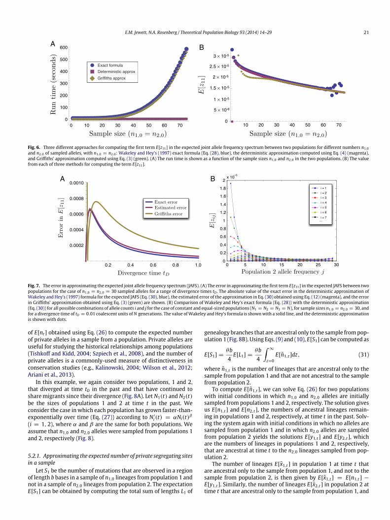
Fig. 6. Three different approaches for computing the first term E[z11] in the expected joint allele frequency spectrum between two populations for different numbers n1,0and n2,0 of sampled alleles, with n1,0 = n2,0: Wakeley and Hey’s (1997) exact formula (Eq. (28), blue), the deterministic approximation computed using Eq. (4) (magenta),and Griffiths’ approximation computed using Eq. (3) (green). (A) The run time is shown as a function of the sample sizes n1,0 and n2,0 in the two populations. (B) The valuefrom each of three methods for computing the term E[z11].
Fig. 7. The error in approximating the expected joint allele frequency spectrum (JAFS). (A) The error in approximating the first term E[z11] in the expected JAFS between twopopulations for the case of n1,0 = n2,0 = 30 sampled alleles for a range of divergence times tD . The absolute value of the exact error in the deterministic approximation ofWakeley and Hey’s (1997) formula for the expected JAFS (Eq. (30), blue), the estimated error of the approximation in Eq. (30) obtained using Eq. (12) (magenta), and the errorin Griffiths’ approximation obtained using Eq. (3) (green) are shown. (B) Comparison of Wakeley and Hey’s exact formula (Eq. (28)) with the deterministic approximation(Eq. (30)) for all possible combinations of allele counts i and j for the case of constant and equal-sized populations (N1 = N2 = N3 = N), for sample sizes n1,0 = n2,0 = 30, andfor a divergence time of tD = 0.01 coalescent units of N generations. The value ofWakeley and Hey’s formula is shownwith a solid line, and the deterministic approximationis shown with dots.
of E[nt ] obtained using Eq. (26) to compute the expected numberof private alleles in a sample from a population. Private alleles areuseful for studying the historical relationships among populations(Tishkoff and Kidd, 2004; Szpiech et al., 2008), and the number ofprivate alleles is a commonly-used measure of distinctiveness inconservation studies (e.g., Kalinowski, 2004; Wilson et al., 2012;Ariani et al., 2013).
In this example, we again consider two populations, 1 and 2,that diverged at time tD in the past and that have continued toshare migrants since their divergence (Fig. 8A). Let N1(t) and N2(t)be the sizes of populations 1 and 2 at time t in the past. Weconsider the case in which each population has grown faster-than-exponentially over time (Eq. (27)) according to N ′
i (t) = αNi(t)β(i = 1, 2), where α and β are the same for both populations. Weassume that n1,0 and n2,0 alleles were sampled from populations 1and 2, respectively (Fig. 8).
5.2.1. Approximating the expected number of private segregating sitesin a sample
Let S1 be the number of mutations that are observed in a regionof length b bases in a sample of n1,0 lineages from population 1 andnot in a sample of n2,0 lineages from population 2. The expectationE[S1] can be obtained by computing the total sum of lengths L1 of
genealogy branches that are ancestral only to the sample frompop-ulation 1 (Fig. 8B). Using Eqs. (9) and (10), E[S1] can be computed as
E[S1] =θb4
E[L1] =θb4
∞
z=0E[n1,z]dz, (31)
where n1,t is the number of lineages that are ancestral only to thesample from population 1 and that are not ancestral to the samplefrom population 2.
To compute E[n1,t ], we can solve Eq. (26) for two populationswith initial conditions in which n1,0 and n2,0 alleles are initiallysampled from populations 1 and 2, respectively. The solution givesus E[n1,t ] and E[n2,t ], the numbers of ancestral lineages remain-ing in populations 1 and 2, respectively, at time t in the past. Solv-ing the system again with initial conditions in which no alleles aresampled from population 1 and in which n2,0 alleles are sampledfrom population 2 yields the solutions E[y1,t ] and E[y2,t ], whichare the numbers of lineages in populations 1 and 2, respectively,that are ancestral at time t to the n2,0 lineages sampled from pop-ulation 2.
The number of lineages E[x1,t ] in population 1 at time t thatare ancestral only to the sample from population 1, and not to thesample from population 2, is then given by E[x1,t ] = E[n1,t ] −
E[y1,t ]. Similarly, the number of lineages E[x2,t ] in population 2 attime t that are ancestral only to the sample from population 1, and

22 E.M. Jewett, N.A. Rosenberg / Theoretical Population Biology 93 (2014) 14–29
Fig. 8. Comparison of stochastic and deterministic coalescent models for computing the expected number of mutations that are private to a sample of alleles from apopulation. In each model, two populations, 1 and 2, diverge at time tD in the past. Samples of sizes n1,0 and n2,0 are taken from populations 1 and 2, respectively. (A) Theclassical stochastic coalescent model. Orange crosses indicate mutations that occur on lineages that are ancestral only to the sample from population 1. (B) The deterministiccoalescent model. The red region indicates lineages ancestral only to the sample from population 1, the blue region indicates lineages ancestral only to the sample frompopulation 2, and the purple region indicates lineages ancestral to both samples. The width of the shaded region of each color in each population at a fixed time t is theexpected number of lineages of the given type in the given population at that time. The total sum of branch lengths on which a mutation ancestral only to the sample frompopulation 1 can occur is the area of the region shaded in red.
Fig. 9. Comparisonwith simulations of analytical approximations of E[S1] obtainedusing Eq. (31) with simulations.
not to the sample from population 2, is given by E[x2,t ] = E[n2,t ]−
E[y2,t ]. The expected total number of lineages ancestral only to thesample frompopulation 1 is given by E[n1,t ] = E[x1,t ]+E[x2,t ]. Theexpectation E[S1] is then obtained by plugging the value of E[n1,t ]
into Eq. (31) for a given choice of θ and b.Theorem 2.1 implies that Eq. (31) is exact if E[n1,t ] is exact.
However, because the differential equation in Eq. (26) is approx-imate, there will be a small amount of error in our computation ofE[S1]. We examine this error empirically in Section 5.2.2.
5.2.2. The accuracy of the approximation in Eq. (31)To examine the error in Eq. (31) that arises from the approxi-
mation in Eq. (26), we compared the analytical results obtained us-ing Eqs. (26) and (31) to simulations. Simulations were performedby sampling genealogies from the Markov chain with transitionprobabilities given by Eq. (22) using an approach similar to thatdescribed by Jewett et al. (2012). We discuss the simulation proce-dure in more detail in Appendix F.
Approximations of E[S1] appear in Fig. 9 for various sample sizesn1,0 and n2,0, along with simulated values for comparison. In ourcomputations and simulations, we have taken N1(0) = N2(0) = 1,and we have set N3(t) = N1(tD) + N2(tD) at the divergence timetD. The other parameters were chosen in order to model moderatelevels of faster-than-exponential growth and migration: α = 5,β = 10, and m12 = m21 = 10. Because the parameters band θ in our model only affect the computed values of E[S1] bya constant scaling factor, we set each of these values to unity forsimplicity (b = 1 and θ = 1). From Fig. 9, it can be seen that theapproximation is very accurate over the range of parameter values,even when the sample sizes are small.
5.3. The time to the first inter-sample coalescent event
In the examples in Sections 5.1 and 5.2, we have used the ap-proximation nt ≈ E[nt ] to compute expected values. However, theapproximation can also be used to derive approximate probabil-ity distributions. For example, Volz et al. (2009) used a version ofthe approximation in Eq. (4) to compute the joint distribution ofcoalescent waiting times among a set of sampled lineages in a sin-gle population of variable size (Volz et al., 2009, Eq. (12)). Here, weconsider the related problem of computing the distribution of thetime until the first coalescent event between two different sets ofsampled alleles in a model with two populations of variable sizewith migration among them (Fig. 10).
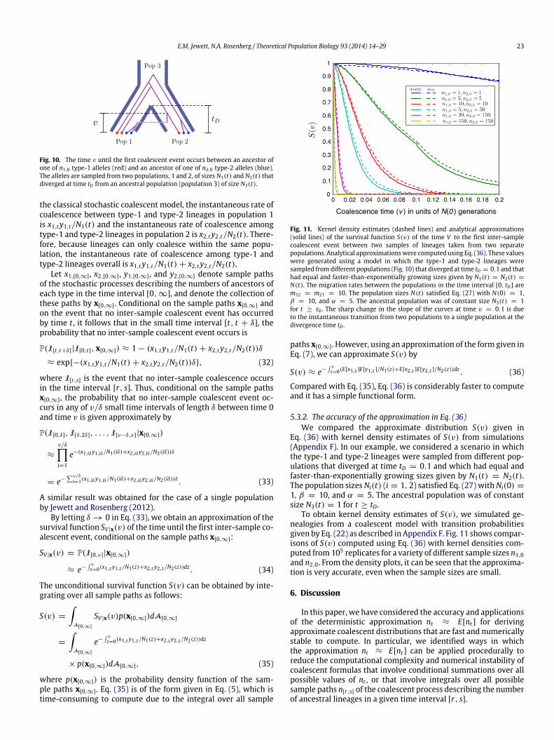
We again consider a model in which two populations divergeat time tD from a common ancestral population (Fig. 10). Considera sample of n1,0 alleles from one or both of the populations, anddenote these as ‘‘type-1’’ alleles. Suppose that a second sample ofn2,0 alleles is taken from one or both populations and denote theseas ‘‘type-2’’ alleles. We refer to lineages ancestral to type-1 allelesas ‘‘type-1’’ lineages, and we refer to lineages ancestral to type-2alleles as ‘‘type-2’’ lineages. We are interested in computing thedistribution of the random time V until the first coalescent eventoccurs between a type-1 lineage and a type-2 lineage when themigration rates between the populations are nonzero. We refer toa coalescent event between a type-1 lineage and a type-2 lineageas an inter-sample coalescent event.
Inter-sample coalescence times have a number of applications.For example, when the type-1 and type-2 alleles are sampled fromtwo different populations, the time to the first inter-sample coa-lescent event can be used to estimate the divergence time of thetwo populations (Takahata and Nei, 1985; Mossel and Roch, 2010;Liu et al., 2010; Jewett and Rosenberg, 2012). When n1,0 = 1, thedistribution of the time to the first inter-sample coalescent eventcan be used to compute the probability of observing a new haplo-type, conditional on an observed set of n2,0 haplotypes (Paul andSong, 2010), or to predict the accuracy of imputing genotypes ona haplotype using a reference panel of existing haplotypes (Jew-ett et al., 2012; Huang et al., 2013). The expected time of the firstinter-sample coalescent eventwas computed in amigrationmodelusing simulations by Takahata and Slatkin (1990). Here, we showhow a simple approximate analytical distribution can be derivedusing Eq. (26).
5.3.1. Approximating the distribution of the inter-sample coalescencetime
At time t in the past, suppose that x1,t type-1 lineages and y1,ttype-2 lineages remain in population 1 and suppose that x2,t type-1 lineages and y2,t type-2 lineages remain in population 2. Under
E.M. Jewett, N.A. Rosenberg / Theoretical Population Biology 93 (2014) 14–29 23
Fig. 10. The time v until the first coalescent event occurs between an ancestor ofone of n1,0 type-1 alleles (red) and an ancestor of one of n2,0 type-2 alleles (blue).The alleles are sampled from two populations, 1 and 2, of sizes N1(t) and N2(t) thatdiverged at time tD from an ancestral population (population 3) of size N3(t).
the classical stochastic coalescent model, the instantaneous rate ofcoalescence between type-1 and type-2 lineages in population 1is x1,ty1,t/N1(t) and the instantaneous rate of coalescence amongtype-1 and type-2 lineages in population 2 is x2,ty2,t/N2(t). There-fore, because lineages can only coalesce within the same popu-lation, the instantaneous rate of coalescence among type-1 andtype-2 lineages overall is x1,ty1,t/N1(t) + x2,ty2,t/N2(t).
Let x1,[0,∞], x2,[0,∞], y1,[0,∞], and y2,[0,∞] denote sample pathsof the stochastic processes describing the numbers of ancestors ofeach type in the time interval [0, ∞], and denote the collection ofthese paths by x[0,∞]. Conditional on the sample paths x[0,∞] andon the event that no inter-sample coalescent event has occurredby time t , it follows that in the small time interval [t, t + δ], theprobability that no inter-sample coalescent event occurs is
P(I[t,t+δ]|I[0,t], x[0,∞]) ≈ 1 − (x1,ty1,t/N1(t) + x2,ty2,t/N2(t))δ
≈ exp{−(x1,ty1,t/N1(t) + x2,ty2,t/N2(t))δ}, (32)
where I[r,s] is the event that no inter-sample coalescence occursin the time interval [r, s]. Thus, conditional on the sample pathsx[0,∞], the probability that no inter-sample coalescent event oc-curs in any of v/δ small time intervals of length δ between time 0and time v is given approximately by
P(I[0,δ], I[δ,2δ], . . . , I[v−δ,v]|x[0,∞])
≈
v/δi=1
e−(x1,iδy1,iδ/N1(iδ)+x2,iδy2,iδ/N2(iδ))δ
= e−v/δ
i=1(x1,iδy1,iδ/N1(iδ)+x2,iδy2,iδ/N2(iδ))δ. (33)
A similar result was obtained for the case of a single populationby Jewett and Rosenberg (2012).
By letting δ → 0 in Eq. (33), we obtain an approximation of thesurvival function SV |x(v) of the time until the first inter-sample co-alescent event, conditional on the sample paths x[0,∞]:
SV |x(v) = P(I[0,v]|x[0,∞])
≈ e− vz=0(x1,zy1,z/N1(z)+x2,zy2,z/N2(z))dz . (34)
The unconditional survival function S(v) can be obtained by inte-grating over all sample paths as follows:
S(v) =
A[0,∞]
SV |x(v)p(x[0,∞])dA[0,∞]
=
A[0,∞]
e− vz=0(x1,zy1,z/N1(z)+x2,zy2,z/N2(z))dz
× p(x[0,∞])dA[0,∞], (35)
where p(x[0,∞]) is the probability density function of the sam-ple paths x[0,∞]. Eq. (35) is of the form given in Eq. (5), which istime-consuming to compute due to the integral over all sample
Fig. 11. Kernel density estimates (dashed lines) and analytical approximations(solid lines) of the survival function S(v) of the time V to the first inter-samplecoalescent event between two samples of lineages taken from two separatepopulations. Analytical approximationswere computed using Eq. (36). These valueswere generated using a model in which the type-1 and type-2 lineages weresampled fromdifferent populations (Fig. 10) that diverged at time tD = 0.1 and thathad equal and faster-than-exponentially growing sizes given by N1(t) = N2(t) =
N(t). The migration rates between the populations in the time interval [0, tD] arem12 = m21 = 10. The population sizes N(t) satisfied Eq. (27) with N(0) = 1,β = 10, and α = 5. The ancestral population was of constant size N3(t) = 1for t ≥ tD . The sharp change in the slope of the curves at time v = 0.1 is dueto the instantaneous transition from two populations to a single population at thedivergence time tD .
paths x[0,∞]. However, using an approximation of the form given inEq. (7), we can approximate S(v) by
S(v) ≈ e− vz=0(E[x1,z ]E[y1,z ]/N1(z)+E[x2,z ]E[y2,z ]/N2(z))dz . (36)
Compared with Eq. (35), Eq. (36) is considerably faster to computeand it has a simple functional form.
5.3.2. The accuracy of the approximation in Eq. (36)We compared the approximate distribution S(v) given in
Eq. (36) with kernel density estimates of S(v) from simulations(Appendix F). In our example, we considered a scenario in whichthe type-1 and type-2 lineages were sampled from different pop-ulations that diverged at time tD = 0.1 and which had equal andfaster-than-exponentially growing sizes given by N1(t) = N2(t).The population sizes Ni(t) (i = 1, 2) satisfied Eq. (27) with Ni(0) =
1, β = 10, and α = 5. The ancestral population was of constantsize N3(t) = 1 for t ≥ tD.
To obtain kernel density estimates of S(v), we simulated ge-nealogies from a coalescent model with transition probabilitiesgiven by Eq. (22) as described in Appendix F. Fig. 11 shows compar-isons of S(v) computed using Eq. (36) with kernel densities com-puted from105 replicates for a variety of different sample sizes n1,0and n2,0. From the density plots, it can be seen that the approxima-tion is very accurate, even when the sample sizes are small.
6. Discussion
In this paper, we have considered the accuracy and applicationsof the deterministic approximation nt ≈ E[nt ] for derivingapproximate coalescent distributions that are fast and numericallystable to compute. In particular, we identified ways in whichthe approximation nt ≈ E[nt ] can be applied procedurally toreduce the computational complexity and numerical instability ofcoalescent formulas that involve conditional summations over allpossible values of nt , or that involve integrals over all possiblesample paths n[r,s] of the coalescent process describing the numberof ancestral lineages in a given time interval [r, s].

24 E.M. Jewett, N.A. Rosenberg / Theoretical Population Biology 93 (2014) 14–29
We have considered two different kinds of approximation. InSections 2 and 3, we considered the approximation of nt by its ex-pected value E[nt ]. In Section 4, we considered a second kind ofapproximation: approximate formulas for E[nt ]. The first approxi-mation, of nt by E[nt ], holds whenever the behavior of nt is nearlydeterministic. As we showed in Lemma B.1, this deterministic be-havior occurs in the limit as t → 0 and as t → ∞. By contrast,the range of values over which any given approximation of E[nt ]
is valid depends on the approximation that is used. For instance,in Fig. 3, we saw that the approximate function in Eq. (18) is sen-sible in the limit as t → 0 and as t → ∞, whereas the simplerapproximation in Eq. (17) is sensible only in the limit as t → 0.
To facilitate the application of these approximations in prac-tice, we showed that approximate coalescent formulas of the formgiven in Eq. (4) converge to their true values as t → 0 and ast → ∞ under simple assumptions. We also derived an approx-imate expression for the error in these deterministic approxima-tions (Eq. (11)). This approximate expression for the error can beused in practice to evaluate when any given approximate formulaof the form given in Eq. (4) is accurate.
We obtained approximate formulas for E[nt ] in the case of mul-tiple populations with time-varying sizes and migration amongthem (Eq. (26)). These approximations were produced by extend-ing differential equations for E[nt ] derived for the case of a sin-gle panmictic population by Slatkin and Rannala (1997), Volz et al.(2009), andMaruvka et al. (2011). The approximations of E[nt ] thatwe obtained facilitate the derivation of approximate coalescentformulas under complicated demographic scenarios. For example,we showed how approximations of E[nt ] undermigration could beused to approximate the expected number of mutations occurringalong the branches of a genealogy (Section 5.2) or to compute anapproximate distribution of coalescent waiting times (Section 5.3)in demographic models involving multiple populations with mi-gration. Such applications of the approximation nt ≈ E[nt ] are use-ful because deriving exact formulas for coalescent quantities undermodels with both migration and population size changes can bedifficult.
We have described a number of problems to which the approx-imation nt ≈ E[nt ] can be applied. However, we have focused onquantities that can be derived conditional on knowledge of the to-tal number of ancestral lineages remaining at a given time t or overa given time interval [r, s]. Quantities that require knowledge ofthe topology of the coalescent tree relating the ancestral lineages,or of the number of lineages of a particular type, may bemore diffi-cult to derive. It is likely that the approximation nt ≈ E[nt ] can beused to derive a variety of approximate distributions beyond thosediscussed here; however, the approximation nt ≈ E[nt ] must beapplied in a new way for each new class of problem, and the theo-retical accuracy of these applications must be evaluated anew.
One common use of the approximation nt ≈ E[nt ] that we didnot consider in this paper is the inference of the size of a popula-tion at each time in the past by fitting the observed values of ntobtained from a reconstructed genealogy of a set of sampled alle-les to the expected values E[nt ] (t ≥ 0) under a given demographichistory (Frost and Volz, 2010;Maruvka et al., 2011). The theoreticalaccuracy of such fitting approaches is difficult to determine analyt-ically and remains a subject for further work.
The importance of coalescent approximations has been a sub-ject of much recent interest, as it has become increasingly rec-ognized that exact formulas or algorithms can be intractable inpractical scenarios. Many recent studies havemade use of a varietyof simplifying assumptions and approximations to the coalescent,and to coalescent-like problems (Li and Stephens, 2003; McVeanand Cardin, 2005; Marjoram and Wall, 2006; Davison et al., 2009;Paul and Song, 2010; RoyChoudhury, 2011; Li and Durbin, 2011;Sheehan et al., 2013). Our results on the approximation nt ≈ E[nt ]
contribute to this growing toolbox of coalescent-based approxima-tions that can be used to derive functionally simple, computation-ally efficient, and numerically stable approximations of coalescentformulas under a variety of coalescent models. These, and similarkinds of approximations, will become increasingly important formaking population-genetic computations tractable as the sizes ofgenomic data sets continue to grow.
Acknowledgments
We are grateful to Monty Slatkin and Michael DeGiorgio forhelpful comments and discussions. This work was supportedby NSF grant DBI-1146722, NIH grant HG005855, and by theBurroughs Wellcome Fund.
Appendix A. Proof of Theorem 2.1
Proof. Let ([r, s], L, λ) denote the measure space defined on theinterval [r, s] with the Lebesgue σ -algebra on [r, s] and Lebesguemeasure λ. Let A[r,s] denote the space of sample paths n[r,s] of thestochastic process nt over the time interval [r, s], and define themeasure space (A[r,s], S, p), where S is the σ -algebra generatedby the process nt and p is the probability distribution of samplepaths on A[r,s]. We assume that (A[r,s], S, p) is complete, or if not,we assume that it is equal to its completion, which exists by theCompletion Theorem (Rudin, 1975, p. 29). We have
E[L[r,s]] = E s
z=rnzdz
=
A[r,s]
s
z=rnzp(n[r,s])dz dA[r,s]. (A.1)
Tonelli’s theorem (DiBenedetto, 2002, Theorem 14.2, p. 148) statesthat the integrals on the right-hand side of Eq. (A.1) can beexchanged if ([r, s], L, λ) and (A[r,s], S, p) are complete σ -finitemeasure spaces and if nzp(n[r,s]) is a nonnegative measurablefunction on [r, s]×A[r,s]. The function nz is a positive step functionon [r, s] and it is therefore measurable because a measurablefunction can be defined as a limit of step functions (Atkinson andHan, 2009, p. 17). The density function p(n[r,s]) is also positiveand measurable because probability density functions are positiveand measurable by definition (Tao, 2011, p. 193). Therefore, theproduct nzp(n[r,s]) is positive and it is measurable because theproduct of measurable functions is measurable (Franks, 2009, Page48, Exercise 3.1.11). The space ([r, s], L, λ) is complete becausethe Lebesgue σ -algebra combinedwith the Lebesguemeasure on asubset of the real numbers forms a complete measure space (Mas-Colell, 1989, p. 23), and (A[r,s], S, p) is complete by assumption.Because λ([r, s]) = s − r < ∞ and p(A[r,s]) = 1 < ∞, themeasure spaces ([r, s], L, λ) and (A[r,s], S, p) are both sets of finitemeasure, and are therefore σ -finite by definition (DiBenedetto,2002, p.71). Therefore, it follows that the integrals in Eq. (A.1) canbe exchanged by Tonelli’s Theorem, yielding
E[L[r,s]] =
A[r,s]
s
z=rnzp(n[r,s])dz dA[r,s]
=
s
z=r
A[r,s]
nzp(n[r,s])dA[r,s] dz
=
s
z=rE[nz]dz, (A.2)
which completes the proof. �
Appendix B. A lemma for proving Theorem 3.1
In this section we present a lemma that is necessary for prov-ing Theorem 3.1. The lemma states that the number of lineages nt

E.M. Jewett, N.A. Rosenberg / Theoretical Population Biology 93 (2014) 14–29 25
that are ancestral to a set of n0 sampled lineages approaches its ex-pected value E[nt ] as t → 0 and as t → ∞. Specifically, we showthat the random variable nt − E[nt ] converges in probability to 0as t → 0 and as t → ∞. We first show that Var(nt) → 0 as t → 0and as t → ∞ for fixed n0 in a population of arbitrary size N(t).
Lemma B.1. Consider a panmictic population of variable size N(t)such that limt→0
tz=0
1N(z)dz = 0 and limt→∞
tz=0
1N(z)dz = ∞.
For a fixed number, n0, of lineages sampled at time t = 0 from thispopulation, Var(nt) → 0 as t → 0 and as t → ∞.
Proof. Tavaré (1984, p. 131) showed that the moments of nt in apanmictic population of constant effective size N can be obtainedusing the function
E[(nt)[k]] =
n0i=k
(2i − 1)
i − 1k − 1
i(k−1)(n0)[i]
(n0)(i)e−i(i−1)t/2, (B.1)
where E[(nt)[k]|n0] is the kth factorial moment of nt , n[i] = n!/(n−
i)! and n(i) = (n−1+ i)!/(n−1)!, andwhere time t is in coalescentunits of N generations.
Chen and Chen (2013) noted that this formula can be extendedto the case of a population of variable size N(t) using a resultfrom Griffiths and Tavaré (1994). Specifically, Griffiths and Tavaréshowed that in a population of variable size N(t), nt has thesame distribution as the number nτ(t) of ancestral lineages at timeτ(t) =
tz=0
1N(z)dz in a population of constant size one. Thus, in a
population of variable size N(t), Eq. (B.1) becomes
E[(nt)[k]] =
n0i=k
(2i − 1)
i − 1k − 1
i(k−1)(n0)[i]
(n0)(i)e−i(i−1)τ (t)/2, (B.2)
where τ(t) = tz=0
1N(z)dz, and where t is in units of generations.
Using the definitions (nt)[2] = n2t − nt and (nt)[1] = nt , we can
write
Var(nt) = E[n2t ] − E[nt ]
2
= E[(nt)[2]] + E[(nt)[1]] − E[(nt)[1]]2, (B.3)
where, from Eq. (B.2), we have
E[(nt)[2]] =
n0i=2
(2i − 1)(i − 1)i(n0)[i]
(n0)(i)e−
i2
τ(t) (B.4)
and
E[(nt)[1]] =
n0i=1
(2i − 1)(n0)[i]
(n0)(i)e−
i2
τ(t)
. (B.5)
By assumption, we have τ(t) → ∞ as t → ∞. Since e−
i2
τ(t)
→
0 as τ(t) → ∞ for i ≥ 2, it follows from Eq. (B.4) that E[(nt)[2]] →
0 as t → ∞. Similarly, since n[1] = n(1), Eq. (B.5) yields
E[(nt)[1]] = 1 +
n0i=2
(2i − 1)(n0)[i]
(n0)(i)e−
i2
τ(t)
= 1 + O(e−τ(t)), (B.6)
from which it follows that E[(nt)[1]|n0] → 1 as t → ∞. Thus,Var(nt) → 0 as t → ∞ by plugging the limiting values ofEqs. (B.4) and (B.5) into the right-hand side of Eq. (B.3).
To obtain the limiting behavior of Var(nt) as t → 0, we can
use the fact that e−
i2
τ(t)
= 1 −
i2
τ(t) + O(τ (t)2). Thus, from
Eq. (B.4), we have
E[(nt)[2]]
=
n0i=2
(2i − 1)(i − 1)i(n0)[i]
(n0)(i)
1 −
i2
τ(t) + O(τ (t)2)
=
n0i=2
(2i − 1)(i − 1)i(n0)[i]
(n0)(i)
− τ(t)n0i=2
(2i − 1)(i − 1)i(n0)[i]
(n0)(i)
i2
+ O(τ (t)2)
= n02− n0 − τ(t)
n0i=2
(2i − 1)i(i − 1)
×(n0)[i]
(n0)(i)
i2
+ O(τ (t)2), (B.7)
where the three terms in the second equality correspond to thethree terms in brackets in the first equality. The first term, n2
0 − n0,in the third equality is obtained by noting that the first term in thesecond equality is equal to E[(n0)[2]] = n2
0 − n0 (Eq. (B.4)).Similarly, from Eq. (B.5) we have
E[(nt)[1]] =
n0i=1
(2i − 1)(n0)[i]
(n0)(i)
1 −
i2
τ(t) + O(τ (t)2)
= n0 − τ(t)n0i=1
(2i − 1)(n0)[i]
(n0)(i)
i2
+ O(τ (t)2)
= n0 − τ(t)n0
2
+ O(τ (t)2), (B.8)
where the third equality is obtained by noting that the second termin the second equality is equal to half the expression for E[(nt)[2]]
evaluated at time t = 0; it is therefore equal to n0
2
. Squaring
Eq. (B.8) gives
E[(nt)[1]]2
= n20 − 2n0τ(t)
n0
2
+ O(τ (t)2). (B.9)
Thus, by plugging Eqs. (B.7)–(B.9) into Eq. (B.3), we obtain
Var(nt) = n20 − n0 + O(τ (t)) + n0 + O(τ (t)) − n2
0 + O(τ (t))
= O(τ (t)). (B.10)
Here, we have used the fact that τ(t)2 = O(τ (t)). The right-hand side of Eq. (B.10) follows from the linearity of ordernotation (Miller, 2006, p. 21). Thus, it follows from our assumptionthat N(t) varies in such a way that τ(t) → 0 as t → 0 thatVar(nt) → 0 as t → 0 for fixed values of n0. �
We now show that nt − E[nt ] converges in probability to 0 ast → 0 and as t → ∞.
Lemma B.2. Consider a panmictic population of variable size N(t) attime t, such that limt→0
tz=0
1N(z)dz = 0 and limt→∞
tz=0
1N(z)dz =
∞. Suppose that n0 lineages are sampled from this population andconsider the number of ancestral lineages nt at time t in the past.Under the coalescent model, the random variable nt −E[nt ] convergesin probability to 0 as t → 0 and as t → ∞.
Proof. The quantity nt is bounded above by n0 and below byunity. Thus, nt has finite mean and variance and therefore satisfiesChebyshev’s inequality (Ross, 2007, p. 77). In particular, for anyϵ > 0, direct application of Chebyshev’s inequality gives
Pr(|nt − E[nt ]| > ϵ) ≤Var(nt)
ϵ2. (B.11)

26 E.M. Jewett, N.A. Rosenberg / Theoretical Population Biology 93 (2014) 14–29
In Lemma B.1 we showed that for fixed n0, Var(nt) → 0 as t → 0and as t → ∞. By the sandwich theorem applied to Eq. (B.11), itfollows that Pr(|nt − E[nt ]| > ϵ) → 0 as t → 0 and as t → ∞.Thus, by the definition of convergence in probability (Casella andBerger, 2002, p. 232), nt − E[nt ] converges in probability to 0. �
Appendix C. Proof of Theorem 3.1
Here, we prove that the deterministic approximation (Eq. (4))is accurate as t → 0 and as t → ∞ for fixed n0.
Proof. To prove Theorem 3.1, we can expand f (x|nt) around thepoint E[nt ]. The first term in this expansion is simply our approx-imation f (x|E[nt ]), and we can show that the higher-order termsin the expansion converge to zero as t → 0 and as t → ∞.
By the second-order mean value theorem (Hendrix and Tóth,2010, p. 41), we have
f (x|nt) = f (x|E[nt ]) + ∇nt f (x|E[nt ])(nt − E[nt ])
+ (nt − E[nt ])T 12Hnt [f (x|ct)](nt − E[nt ]), (C.1)
where Hnt [f (x|ct)] is the Hessian of f (x|nt) with respect to ntevaluated at a point ct given by ct = E[nt ]+q(nt −E[nt ]) for someq ∈ [0, 1]. Taking the expectation of both sides with respect to ntand noting that f (x) =
nt f (x|nt) Pr(nt) = E[f (x|nt)], we obtain
f (x) = E[f (x|nt)]
= f (x|E[nt ]) +12E
(nt − E[nt ])
THnt [f (x|ct)]
× (nt − E[nt ]), (C.2)
where the expectation of the second term in Eq. (C.1) is equal tozero because E[nt − E[nt ]] = 0. Rearranging Eq. (C.2) and takingabsolute values gives
|f (x) − f (x|E[nt ])|
=
E 12(nt − E[nt ])
THnt [f (x|ct)](nt − E[nt ])
=
E12
ki=1
kj=1
(ni,t − E[ni,t ])(nj,t − E[nj,t ])
×∂2
∂ni,t∂nj,tf (x|ct)
. (C.3)
To prove that f (x|E[nt ]) converges uniformly to f (x) on D ast → 0 and as t → ∞, we can bound the right-hand side of Eq. (C.3)and show that this bounded quantity goes to zero as t → 0 and ast → ∞ for all x ∈ D. From Eq. (C.3), we have
|f (x) − f (x|E[nt ])|
≤12E
k
i=1
kj=1
(ni,t − E[ni,t ])(nj,t − E[nj,t ])
×
∂2
∂ni,t∂nj,tf (x|ct)
≤ Mk
i=1
kj=1
E(ni,t − E[ni,t ])(nj,t − E[nj,t ])
. (C.4)
Here, M = maxi,j∈{1,...,k} supc∈N12 |
∂2
∂ni,t ∂nj,tf (x|c)| exists on D × N
because we have assumed that the second-order partial deriva-tives ∂2
∂ni,t ∂nj,tf (x|nt) are bounded. Considering the summandon the
right-hand side of Eq. (C.4), we have
E[|(ni,t − E[ni,t ]) (nj,t − E[nj,t ])|]
≤ E[|ni,t − E[ni,t ]||nj,t − E[nj,t ]|]
≤ ni,0E[|nj,t − E[nj,t ]|], (C.5)
because |ni,t − E[ni,t ]| ≤ ni,0. Now, to show that the term on theright-hand side in Eq. (C.5) converges to 0 as t → 0 and as t → ∞,we can use a convergence theorem from Van der Vaart (2000, The-orem 2.20). This theorem states that if a sequence Wn of randomvariables converges in probability toW in the limit asn → ∞, thenE[Wn] → E[W ] as n → ∞, whenever Wn is asymptotically uni-formly integrable. Thus, in Eq. (C.5), E[|nj,t − E[nj,t ]|] → E[0] = 0if |ni,t − E[ni,t ]| is asymptotically uniformly integrable.
A sequence of random variablesWn is asymptotically uniformlyintegrable (Van der Vaart, 2000, p. 17) if
limM→∞
lim supn→∞
E[|Wn|1{|Wn|>M}] = 0, (C.6)
where 1{|Wn|>M} is the indicator random variable with 1{|Wn|>M} =
1 if |Wn| > M and 1{|Wn|>M} = 0, otherwise. From this defini-tion, it can be seen that |nj,t − E[nj,t ]| is asymptotically uniformlyintegrable because E[|nj,t − E[nj,t ]|1|nj,t−E[nj,t ]|>M ] = 0 wheneverM > sup |nj,t − E[nj,t ]| = nj,0. Therefore, the right-hand side ofEq. (C.5) converges to zero as t → 0 and as t → ∞ for all x ∈ Dand for fixed n0 ∈ N . By the sandwich theorem, it follows thatE[|(ni,t − E[ni,t ])(nj,t − E[nj,t ])|] → 0 as t → 0 and as t → ∞.From a second application of the sandwich theorem, it follows thatthe left-hand-side of Eq. (C.4), |f (x) − f (x|E[nt ])|, converges uni-formly to 0 for all x in D as t → 0 and as t → ∞. �
Appendix D. Approximate error in the deterministic approxi-mation
Eq. (C.3) in the proof of Theorem 3.1 allows us to obtain an es-timate of the error |f (x) − f (x|E[nt ])| in the deterministic approx-imation f (x) ≈ f (x|E[nt ]). From Eq. (C.3), we have
|f (x) − f (x|E[nt ])| =
12k
i=1
kj=1
E(ni,t − E[ni,t ])(nj,t − E[nj,t ])
×∂2
∂ni,t∂nj,tf (x|ct)
. (D.1)
Now, we showed in Lemma B.2 that ni,t − E[ni,t ] converges inprobability to 0 as t → 0 and as t → ∞. It follows that P(∥nt −
E[nt ]∥ > ϵ) → 0 for any ϵ > 0 as t → 0 and as t → ∞. Thus,recalling that ct = E[nt ]+ q(nt −E[nt ]), we have P(∥[ct −E[nt ]]∥
> ϵ) = P(∥[nt − E[nt ]]∥ > ϵ/q) → 0 as t → 0 and as t → ∞.Therefore, as t → 0 and as t → ∞, we can make the approxima-tion ct ≈ E[nt ]. Using the approximation ct ≈ E[nt ] as t → 0 andas t → ∞, and approximating the expectation of a product by theproduct of the expectations, we obtain
|f (x) − f (x|E[nt ])| ≈
12k
i=1
kj=1
E[(ni,t − E[ni,t ])(nj,t − E[nj,t ])]
× E
∂2
∂ni,t∂nj,tf (x|E[nt ])
=
12k
i=1
kj=1
Cov(ni,t , nj,t)∂2
∂ni,t∂nj,tf (x|E[nt ])
. (D.2)
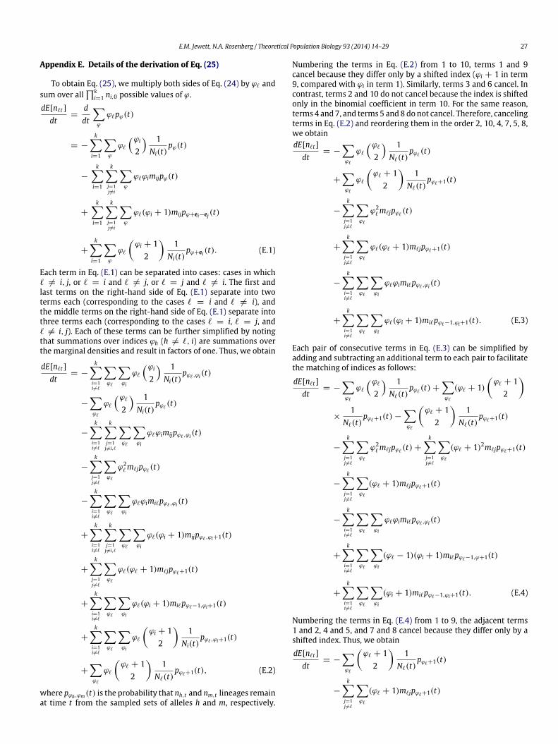
E.M. Jewett, N.A. Rosenberg / Theoretical Population Biology 93 (2014) 14–29 27
Appendix E. Details of the derivation of Eq. (25)
To obtain Eq. (25), we multiply both sides of Eq. (24) by ϕℓ andsum over all
ki=1 ni,0 possible values of ϕ.
dE[nℓt ]
dt=
ddt
ϕ
ϕℓpϕ(t)
= −
ki=1
ϕ
ϕℓ
ϕi
2
1Ni(t)
pϕ(t)
−
ki=1
kj=1j=i
ϕ
ϕℓϕimijpϕ(t)
+
ki=1
kj=1j=i
ϕ
ϕℓ(ϕi + 1)mijpϕ+ei−ej(t)
+
ki=1
ϕ
ϕℓ
ϕi + 1
2
1
Ni(t)pϕ+ei(t). (E.1)
Each term in Eq. (E.1) can be separated into cases: cases in whichℓ = i, j, or ℓ = i and ℓ = j, or ℓ = j and ℓ = i. The first andlast terms on the right-hand side of Eq. (E.1) separate into twoterms each (corresponding to the cases ℓ = i and ℓ = i), andthe middle terms on the right-hand side of Eq. (E.1) separate intothree terms each (corresponding to the cases ℓ = i, ℓ = j, andℓ = i, j). Each of these terms can be further simplified by notingthat summations over indices ϕh (h = ℓ, i) are summations overthe marginal densities and result in factors of one. Thus, we obtain
dE[nℓt ]
dt= −
ki=1i=ℓ
ϕℓ
ϕi
ϕℓ
ϕi
2
1Ni(t)
pϕℓ,ϕi(t)
−
ϕℓ
ϕℓ
ϕℓ
2
1Ni(t)
pϕℓ(t)
−
ki=1i=ℓ
kj=1j=i,ℓ
ϕℓ
ϕi
ϕℓϕimijpϕℓ,ϕi(t)
−
kj=1j=ℓ
ϕℓ
ϕ2ℓmℓjpϕℓ
(t)
−
ki=1i=ℓ
ϕℓ
ϕi
ϕℓϕimiℓpϕℓ,ϕi(t)
+
ki=1i=ℓ
kj=1j=i,ℓ
ϕℓ
ϕi
ϕℓ(ϕi + 1)mijpϕℓ,ϕi+1(t)
+
kj=1j=ℓ
ϕℓ
ϕℓ(ϕℓ + 1)mℓjpϕℓ+1(t)
+
ki=1i=ℓ
ϕℓ
ϕi
ϕℓ(ϕi + 1)miℓpϕℓ−1,ϕi+1(t)
+
ki=1i=ℓ
ϕℓ
ϕi
ϕℓ
ϕi + 1
2
1
Ni(t)pϕℓ,ϕi+1(t)
+
ϕℓ
ϕℓ
ϕℓ + 1
2
1
Nℓ(t)pϕℓ+1(t), (E.2)
where pϕh,ϕm(t) is the probability that nh,t and nm,t lineages remainat time t from the sampled sets of alleles h and m, respectively.
Numbering the terms in Eq. (E.2) from 1 to 10, terms 1 and 9cancel because they differ only by a shifted index (ϕi + 1 in term9, compared with ϕi in term 1). Similarly, terms 3 and 6 cancel. Incontrast, terms 2 and 10 do not cancel because the index is shiftedonly in the binomial coefficient in term 10. For the same reason,terms 4 and 7, and terms 5 and 8 do not cancel. Therefore, cancelingterms in Eq. (E.2) and reordering them in the order 2, 10, 4, 7, 5, 8,we obtaindE[nℓt ]
dt= −
ϕℓ
ϕℓ
ϕℓ
2
1Nℓ(t)
pϕℓ(t)
+
ϕℓ
ϕℓ
ϕℓ + 1
2
1
Nℓ(t)pϕℓ+1(t)
−
kj=1j=ℓ
ϕℓ
ϕ2ℓmℓjpϕℓ
(t)
+
kj=1j=ℓ
ϕℓ
ϕℓ(ϕℓ + 1)mℓjpϕℓ+1(t)
−
ki=1i=ℓ
ϕℓ
ϕi
ϕℓϕimiℓpϕℓ,ϕi(t)
+
ki=1i=ℓ
ϕℓ
ϕi
ϕℓ(ϕi + 1)miℓpϕℓ−1,ϕi+1(t). (E.3)
Each pair of consecutive terms in Eq. (E.3) can be simplified byadding and subtracting an additional term to each pair to facilitatethe matching of indices as follows:
dE[nℓt ]
dt= −
ϕℓ
ϕℓ
ϕℓ
2
1Nℓ(t)
pϕℓ(t) +
ϕℓ
(ϕℓ + 1)
ϕℓ + 12
×
1Nℓ(t)
pϕℓ+1(t) −
ϕℓ
ϕℓ + 1
2
1
Nℓ(t)pϕℓ+1(t)
−
kj=1j=ℓ
ϕℓ
ϕ2ℓmℓjpϕℓ
(t) +
kj=1j=ℓ
ϕℓ
(ϕℓ + 1)2mℓjpϕℓ+1(t)
−
kj=1j=ℓ
ϕℓ
(ϕℓ + 1)mℓjpϕℓ+1(t)
−
ki=1i=ℓ
ϕℓ
ϕi
ϕℓϕimiℓpϕℓ,ϕi(t)
+
ki=1i=ℓ
ϕℓ
ϕi
(ϕℓ − 1)(ϕi + 1)miℓpϕℓ−1,ϕ+1(t)
+
ki=1i=ℓ
ϕℓ
ϕi
(ϕi + 1)miℓpϕℓ−1,ϕi+1(t). (E.4)
Numbering the terms in Eq. (E.4) from 1 to 9, the adjacent terms1 and 2, 4 and 5, and 7 and 8 cancel because they differ only by ashifted index. Thus, we obtaindE[nℓt ]
dt= −
ϕℓ
ϕℓ + 1
2
1
Nℓ(t)pϕℓ+1(t)
−
kj=1j=ℓ
ϕℓ
(ϕℓ + 1)mℓjpϕℓ+1(t)

28 E.M. Jewett, N.A. Rosenberg / Theoretical Population Biology 93 (2014) 14–29
+
ki=1i=ℓ
ϕℓ
ϕi
(ϕi + 1)miℓpϕℓ−1,ϕi+1(t)
= −1
Nℓ(t)E
nℓt
2
−
kj=1j=ℓ
E[nℓt ]mℓj +
ki=1i=ℓ
E[nit ]miℓ
= −1
2Nℓ(t)
E[n2
ℓt ] − E[nℓt ]
+
ki=1i=ℓ
(E[nit ]miℓ − E[nℓt ]mℓi)
= −1
2Nℓ(t)
E[n2
ℓt ] − E[nℓt ]2+ E[nℓt ]
2− E[nℓt ]
+
ki=1i=ℓ
(E[nit ]miℓ − E[nℓt ]mℓi)
= −Var(nℓt)
2Nℓ(t)−
1Nℓ(t)
E[nℓt ]
2
+
ki=1i=ℓ
(E[nit ]miℓ − E[nℓt ]mℓi). (E.5)
This completes the derivation of Eq. (25) from Eq. (24).
Appendix F. Simulation procedure
The accuracy of the approximate expressions in Eqs. (31) and(36) was evaluated by comparing each approximation with esti-mates of the exact values obtained using simulations. The simula-tion procedure that was used to validate each approximation wassimilar to that described elsewhere (Jewett et al., 2012); however,we provide a brief description of the procedure here.
All simulations were performed under a model in which twopopulations of sizes N1(t) and N2(t), respectively, diverged at timetD in the past from an ancestral population of size N3(t). Under thismodel, if a alleles remain at time t in population i, then the addi-tional time ta until a coalescent event occurs among these a lin-eages can be simulated by first sampling the time ta to coalescencein a population of constant size 1, and then rescaling this time ac-cording to the formula τa(t) =
taz=t 1/Ni(z)dz (see the discussion
of time scaling in Section 4.1). In a population of constant size 1,the time ta until a alleles coalesce is exponentially distributedwithmean 1/
a2
generations.
In contrast to coalescence times, waiting times betweenmigra-tion events can be sampled without rescaling time. If a lineagesremain at time t in population i, then the time until one of thesea lineages migrates to the other population j is exponentially dis-tributed withmean 1/(amij), wheremij is the backward rate of mi-gration from population i to population j.
The simulation proceeds as follows. Suppose that n1,0 and n2,0lineages are initially sampled from populations 1 and 2, respec-tively. The time until the first event of any kind (coalescence ormigration) is sampled by sampling the time t1C until the first co-alescence in population 1, the time t2C until the first coalescenceoccurs in population 2, the time t1M until the first migration frompopulation 1 to population 2, and the time t2M until the first mi-gration event from population 2 to population 1. The minimum ofthese times, min{t1C , t1M , t2C , t2M}, is then identified. If tiC (i = 1or 2) is theminimum time, then two lineages from population i arerandomly chosen and combined. If tiM (i = 1 or 2) is the minimumtime, then a lineage in population i is randomly chosen andmovedto population j = i. The current time is set to t = min{t1C , t1M , t2C ,
t2M} and the time until the next event (coalescence or migration)is sampled using the same procedure. This procedure is repeateduntil the time t + min{t1C , t1M , t2C , t2M} exceeds the divergencetime tD. Once t + min{t1C , t1M , t2C , t2M} exceeds tD, all remaininglineages aremerged into the ancestral population of sizeN3(t) and,starting from time tD, coalescence times are sampled until a singlelineage remains.
F.1. Simulating the number of private alleles under migration
To obtain a Monte Carlo estimate of the number of private al-leles in a sample of n1,0 alleles from population 1, we sampled ge-nealogies using the above procedure. For each sampled genealogy,the total sum of lengths L1 of branches ancestral only to the sampleof n1,0 alleles from population 1was computed. E[S1]was obtainedbymultiplying each sampled value of L1 by θb/4 and averaging theresulting values across all replicates. For each combination of pa-rameter values we tested, E[S1] was computed using 104 sampledgenealogies.
F.2. Simulating the time until the first inter-sample coalescent event
To obtain a Monte Carlo estimate the distribution of thetime until the first inter-sample coalescent event occurs betweenn1,0 type-1 lineages and n2,0 type-2 lineages sampled from twopopulations, we sampled genealogies using the above procedure.For each pair of sample sizes n1,0 and n2,0 that we considered, wesimulated 105 genealogies. For each genealogy, we recorded thetime V of the first coalescent event between a type-1 and a type-2 lineage. We then computed kernel density estimates on the 105
sampled values of V using Matlab’s ksdensity function with defaultparameters and with the option ‘function’, ‘survivor’.
References
Ariani, C.V., Pickles, R.S.A., Jordan, W.C., Lobo-Hajdu, G., Rocha, C.F.D., 2013.Mitochondrial DNA andmicrosatellite loci data supporting amanagement planfor a critically endangered lizard from Brazil. Conserv. Genet. 14, 943–951.
Atkinson, K.E., Han,W., 2009. Theoretical Numerical Analysis: a Functional AnalysisFramework. Springer-Verlag, New York.
Bryant, D., Bouckaert, R., Felsenstein, J., Rosenberg, N.A., RoyChoudhury, A., 2012.Inferring species trees directly from biallelic genetic markers: bypassing genetrees in a full coalescent analysis. Mol. Biol. Evol. 29, 1917–1932.
Casella, G., Berger, R.L., 2002. Statistical Inference, second ed. Duxbury Press, PacificGrove, CA.
Chen, H., Chen, K., 2013. Asymptotic distributions of coalescence times andancestral lineage numbers for populations with temporally varying size.Genetics 194, 721–736.
Davison, D., Pritchard, J.K., Coop, G., 2009. An approximate likelihood for geneticdata under a model with recombination and population splitting. Theor. Popul.Biol. 75, 331–345.
Degnan, J.H., 2010. Probabilities of gene trees with intraspecific sampling given aspecies tree. In: Knowles, L.L., Kubatko, L.S. (Eds.), Estimating Species Trees:Practical and Theoretical Aspects. Wiley-Blackwell, Hoboken, NJ, pp. 53–78.
Degnan, J.H., Salter, L.A., 2005. Gene tree distributions under the coalescent process.Evolution 59, 24–37.
DiBenedetto, E., 2002. Real Analysis. Birkhauser, Boston.Donnelly, P., 1984. The transient behaviour of the Moran model in population
genetics. Math. Proc. Cambridge Philos. Soc. 95, 349–358.Efromovich, S., Kubatko, L., 2008. Coalescent time distributions in trees of arbitrary
size. Stat. Appl. Genet. Mol. Biol. 7, Article 2.Franks, J.M., 2009. A (Terse) Introduction to Lebesgue Integration. American
Mathematical Society, Providence, RI.Frost, S.D.W., Volz, E.M., 2010. Viral phylodynamics and the search for an effective
number of infections. Philos. Trans. R. Soc. Lond. B 365, 1879–1890.Griffiths, R.C., 1980. Lines of descent in the diffusion approximation of neutral
Wright–Fisher models. Theor. Popul. Biol. 17, 37–50.Griffiths, R.C., 1984. Asymptotic line-of-descent distributions. J. Math. Biol. 21,
67–75.Griffiths, R.C., 2006. Coalescent lineage distributions. Adv. Appl. Probab. 38,
405–429.Griffiths, R.C., Tavaré, S., 1994. Sampling theory for neutral alleles in a varying
environment. Philos. Trans. R. Soc. Lond. B 29, 403–410.Griffiths, R.C., Tavaré, S., 1998. The age of a mutation in a general coalescent tree.
Stoch. Models 14, 273–295.

E.M. Jewett, N.A. Rosenberg / Theoretical Population Biology 93 (2014) 14–29 29
Gutenkunst, R.N., Hernandez, R.D., Williamson, S.H., Bustamante, C.D., 2009. Infer-ring the joint demographic history of multiple populations from multidimen-sional SNP frequency data. PLoS Genet. 5, e1000695.
Helmkamp, L.J., Jewett, E.M., Rosenberg, N.A., 2012. Improvements to a class ofdistance matrix methods for inferring species trees from gene trees. J. Comput.Biol. 19, 632–649.
Hendrix, E.M.T., Tóth, B.G., 2010. Introduction to Nonlinear and Global Optimiza-tion. Springer, New York.
Huang, L., Buzbas, E.O., Rosenberg, N.A., 2013. Genotype imputation in a coalescentmodel with infinitely-many-sites mutation. Theor. Popul. Biol. 87, 62–74.
Hudson, R.R., Coyne, J.A., 2002. Mathematical consequences of the genealogicalspecies concept. Evolution 56, 1557–1565.
Jewett, E.M., Rosenberg, N.A., 2012. iGLASS: an improvement to the GLASS methodfor estimating species trees from gene trees. J. Comput. Biol. 19, 293–315.
Jewett, E.M., Zawistowski, M., Rosenberg, N.A., Zöllner, S., 2012. A coalescentmodelfor genotype imputation. Genetics 191, 1239–1255.
Kalinowski, S.T., 2004. Counting alleles with rarefaction: private alleles andhierarchical sampling designs. Conserv. Genet. 5, 539–543.
Li, H., Durbin, R., 2011. Inference of human population history from individualwhole-genome sequences. Nature 475, 493–496.
Li, N., Stephens, M., 2003. Modeling linkage disequilibrium and identifyingrecombination hotspots using single-nucleotide polymorphism data. Genetics165, 2213–2233.
Liu, L., Yu, L., Pearl, D.K., 2010. Maximum tree: a consistent estimator of the speciestree. J. Math. Biol. 60, 95–106.
Marjoram, P., Wall, J.D., 2006. Fast ‘‘coalescent’’ simulation. BMC Genet. 7, 16.Maruvka, Y.E., Shnerb, N.M., Bar-Yam, Y., Wakeley, J., 2011. Recovering population
parameters from a single gene genealogy: an unbiased estimator of the growthrate. Mol. Biol. Evol. 28, 1617–1631.
Mas-Colell, A., 1989. The Theory of General Economic Equilibrium: a DifferentiableApproach. Cambridge University Press, New York.
McVean, G.A.T., Cardin, N.J., 2005. Approximating the coalescent with recombina-tion. Philos. Trans. R. Soc. Lond. B 360, 1387–1393.
Miller, P.D., 2006. Applied Asymptotic Analysis. American Mathematical Society,Providence, RI.
Mossel, E., Roch, S., 2010. Incomplete lineage sorting: consistent phylogenyestimation from multiple loci. IEEE/ACM Trans. Comput. Biol. Bioinform. 7,166–171.
Nielsen, R., Hubisz, M.J., Hellmann, I., Torgerson, D., Andrés, A.M., Albrechtsen, A.,Gutenkunst, R., Adams, M.D., Cargill, M., Boyko, A., Indap, A., Bustamante, C.D.,Clark, A.G., 2009. Darwinian and demographic forces affecting human proteincoding genes. Genome Res. 19, 838–849.
Paul, J.S., Song, Y.S., 2010. A principled approach to deriving approximateconditional sampling distributions in population genetics models withrecombination. Genetics 186, 321–338.
Rauch, E.M., Bar-Yam, Y., 2005. Estimating the total genetic diversity of a spatialfield population from a sample and implications of its dependence on habitatarea. Proc. Natl. Acad. Sci. USA 102, 9826–9829.
Reppell, M., Boehnke, M., Zöllner, S., 2012. FTEC: a coalescent simulator formodeling faster than exponential growth. Bioinformatics 28, 1282–1283.
Rosenberg, N.A., 2002. The probability of topological concordance of gene trees andspecies trees. Theor. Popul. Biol. 61, 225–247.
Rosenberg, N.A., 2003. The shapes of neutral gene genealogies in two species:probabilities of monophyly, paraphyly, and polyphyly in a coalescent model.Evolution 57, 1465–1477.
Rosenberg, N.A., Feldman,M.W., 2002. The relationship between coalescence timesand population divergence times. In: Slatkin, M., Veuille, D. (Eds.), ModernDevelopments in Theoretical Population Genetics. Oxford University Press,Oxford, pp. 130–164.
Ross, S., 2007. Introduction to Probability Models, ninth ed. Academic Press, NewYork.
RoyChoudhury, A., 2011. Composite likelihood-based inferences on genetic datafrom dependent loci. J. Math. Biol. 62, 65–80.
Rudin, W., 1975. Real and Complex Analysis. McGraw Hill, New York.Sheehan, S., Harris, K., Song, Y.S., 2013. Estimating variable effective population
sizes from multiple genomes: a sequentially Markov conditional samplingdistribution approach. Genetics 194, 647–662.
Slatkin, M., 2000. Allele age and a test for selection on rare alleles. Philos. Trans. R.Soc. Lond. B 355, 1663–1668.
Slatkin, M., Rannala, B., 1997. Estimating the age of alleles by use of intraallelicvariability. Am. J. Hum. Genet. 60, 447–458.
Szpiech, Z.A., Jakobsson, M., Rosenberg, N.A., 2008. ADZE: a rarefaction approachfor counting alleles private to combinations of populations. Bioinformatics 24,2498–2504.
Takahata, N., 1989. Gene genealogy in three related populations: consistencyprobability between gene and population trees. Genetics 122, 957–966.
Takahata, N., Nei, M., 1985. Gene genealogy and variance of interpopulationalnucleotide differences. Genetics 110, 325–344.
Takahata, N., Slatkin, M., 1990. Genealogy of neutral genes in two partially isolatedpopulations. Theor. Popul. Biol. 38, 331–350.
Tao, T., 2011. An Introduction to Measure Theory. Amerian Mathematical Society,Providence, RI.
Tavaré, S., 1984. Line-of-descent and genealogical processes, and their applicationsin population genetics models. Theor. Popul. Biol. 26, 119–164.
Tishkoff, S.A., Kidd, K.K., 2004. Implications of biogeography of human populationsfor ‘race’ and medicine. Nat. Genet. 36, S21–S27.
Van der Vaart, A.W., 2000. Asymptotic Statistics. Cambridge University Press.Volz, E.M., Kosakovsky Pond, S.L., Ward, M.J., Leigh Brown, A.J., Frost, S.D.W., 2009.
Phylodynamics of infectious disease epidemics. Genetics 183, 1421–1430.Wakeley, J., Hey, J., 1997. Estimating ancestral populationparameters. Genetics 145,
847–855.Watterson, G.A., 1975. On the number of segregating sites in genetical models
without recombination. Theor. Popul. Biol. 7, 256–276.Wilson, A.S., Marra, P.P., Fleischer, R.C., 2012. Temporal patterns of genetic diversity
in Kirtlands warblers (Dendroica kirtlandii), the rarest songbird in NorthAmerica. BMC Ecol. 12, 8.
Wu, Y., 2012. Coalescent-based species tree inference from gene tree topologiesunder incomplete lineage sorting by maximum likelihood. Evolution 66,763–775.