Approximation of Large Probabilistic Networks

by Structured Population Protocols⋆

Michel de Rougemont2 and Mathieu Tracol2

University Paris South, France mdr@lri.fr, mathieu.tracol@lri.fr

Abstract. We consider networks of Markov Decision Processes (MDPs)where each MDP is one of the N nodes of a graph G. The transition prob-abilities of an MDP depend on the states of its direct neighbors in thegraph, and runs operate by selecting a random node and following a ran-dom transition in the chosen device MDP. As the state space of all theconfigurations of the network is exponential in N, classical analysis areunpractical. We study how a polynomial size statistical representationof the system, which gives the densities of the subgraphs of width k, canbe used to analyze its behaviors, generalizing the approximate ModelChecking of an MDP. We propose a Structured Population Protocol asa new Population MDP where states are statistical representations ofthe network, and transitions are inferred from the statistical structure.Our main results show that when we consider large networks, the distri-butions of probability of the statistics vectors of the simulation processapproximates the distributions of probability of the statistics vectors ofthe real process. Moreover, when the network has some regularity, bothreal and approximation processes will converge to the same distributions.

1 Introduction

We consider large networks of probabilistic systems, where each system (or de-vice) is a Markov Decision Process, i.e. a transition system with both non de-terministic and probabilistic transitions. The device MDPs are placed at nodesof the graph of the network with N nodes. A policy σ determines the decisionsfor all device MDPs, and the network itself can be considered as an MDP whosestate space is the set of configurations of the network, of size exponential in N .Given a policy and an initial distribution, we observe a stochastic process onthe set of configurations by selecting a random node and by following a ran-dom transition in the chosen MDP. Sensors networks are typical applicationswhere sensors are nodes of a graph, connected to some neighbors. We considerEvaluation problems which predict the global behavior when a policy is fixed,and Reachability problems which look for possible policies to ensure predictablebehaviors with high probabilities.

Classical Probabilistic Model Checkers such as PRISM [15] answer such ques-tions on simple probabilistic systems. In [7], we presented some techniques to

⋆ Work supported by ANR-07-SESU-013 program of the French Research ComputerSecurity program

1

approximately decide such questions on a given MDP by associating frequencyvectors to runs. Given an MDP with n states, we built its Polytope of frequencyvectors H which represents the k-frequencies of the different states in the runs,in polynomial time. We can then decide if there is a run which approximatelyverifies some Property with high probability with simple geometrical procedures.

Given a network of N device MDPs, the polytope-based method remainsexponential in N . In this paper, we introduce a new approximate method basedon the statistics on graph neighborhoods of depth k of the network. The crucialpoint is that the set of k-statistics has size polynomially bounded in N . A Struc-tured Population Protocol with Decisions (SPPD) will define a new Population-MDP whose states are statistics vectors and where transitions are determinedby the graph. If we fix a precision for the values of the statistics densities, say1%, the number of possible vectors becomes independent of N . The construc-tion of the population-MDP becomes feasible and we can then apply the initialpolytope-based method. In this context, the classical problems are:

– Evaluation problems. Given a fixed policy σ applied to all the device MDPsand an initial distribution C, can we reach configuration C′ with probabilitygreater than λ ? For a propertyP on the runs, decide if P

σ,C [a run satisfies P ] ≥λ where λ ≤ 1 is a threshold value.

– Reachability problem. Is there a policy σ, such that we can we reach con-figuration C′ from configuration C with probability greater than λ ? If thedevice MDPs have two states for example, dead and alive, we may ask ifP

σ,C [more than 80% of the states are alive in a run ] ≥ 12 ?

We map configurations to their statistics, and approach these problems by con-sidering their approximate versions on the population MDP. The approximateEvaluation is: given the statistics of the configuration C, can we reach the statis-tics of configuration C′ with probability greater than λ? The other problems canbe formulated in a similar way. The main results of the paper are:

– The k-SPPD associated to a network of MDPs is itself an MDP (definition4 and proposition 4).

– Bounds on the approximation of the network of MDPs by the k-SPPD(proposition 5 and theorem 1).

– Sufficient conditions for the convergence of the approximate process inducedby the k-SPPD towards the limit of the real process (theorem 2)

– The polytope associated to the k-SPPD approximates the polytope of theclass of statistics policies on the network of MDPs (theorem 3)

In section 2 we present the model of Markov Decision Processes (MDPs) anddefine the k-statistics on graphs. In section 3 we define our model of network ofMDPs. In section 4 we introduce the general model of k-Structured PopulationProtocols with Decisions on a graph (k-SPPD), and we present how to associatea k-SPPD to a network of MDPs. In section 5 we present sufficient conditions forgood approximations of networks of MDPs by our k-SPPDs. The conditions relyon a notion of mixed configurations. We also study the convergence of the ap-proximate process induced by a k-SPPD, and we present the polytope associatedto the set of statistics policies on a network of MDPs.

2

1.1 Comparison with related models

Various theoretical models of networks have been considered in a context ofdistributed computing and statistical physics. Models for distributed comput-ing [3] also include Petri nets [10], computer networks models [14] and cellularautomata [19] which can be seen as a deterministic and synchronous restrictionof our model. In statistical physics, spatial models [9] have similar probabilis-tic transitions associated with physical neighborhoods, in particular the Isingmodel describing models of spins. These statistical models do not integrate thepossibility to take decisions, and the associated processes induce Markov chainson the sets of configurations.

If we restrict to MDPs with no decisions, i.e. to Markov chains, our modellies between the totally non ordered model of population protocols, introducedby Angluin et al in [3], and the totally ordered model of cellular automata. Wedifferentiate from the population protocol model of [3], as structured graphsneighborhoods are chosen according to some statistics, as opposed to pairs ofdevices. Our work is closer to [2] where the authors consider devices distributedon the vertex of a graph with non randomized interactions between couples ofdevices. Cellular automata and dynamical systems consider regular geometriessuch as linear or square grid graphs (see [19,17]), and update all devices syn-chronously. In [1], the model is close to our model of SPP since the updatefunction is asynchronous and uniformly random among the devices, with therestriction that the transition functions are deterministic.

2 Preliminaries

We first review the MDP model and its polytope representation, and we intro-duce a statistical representation of graphs.

2.1 Markov Decision Processes

Let D(S) be the set of distributions on a set S. A Markov Decision Process(MDP) is a triple S = (S, Σ, P ) where S is a finite set of states, Σ is a setof actions, and P : S × Σ × S → [0, 1] is the transition function: P (s, a, t),also written P (t|s, a), is the probability to arrive in t in one step when thecurrent state is s and action a ∈ Σ is chosen for the transition. If action a isnot allowed from state s, P (t|s, a) = 0 for all t ∈ S. A run on S is a finiteor infinite sequence of states. Given a run r and n ∈ N, we write r|n for thesequence of the first n − 1 states in r. A policy on S, see [18], is a functionσ : S → D(Σ) which resolves the non determinism of the system by choosing adistribution on the set of available actions for each state of the MDP (we restrictour model to stationary and possibly randomized policies). A policy σ and aninitial distribution α ∈ D(S) induce a probability distribution P

σ,α on the σ-fieldF of the set of runs, generated by the cones Cρ = r | r|ρ| = ρ, (see [6,18]).When there is no decision for the MDP, i.e. when |Σ| = 1, the MDP is in fact aMarkov chain. See appendix A for an example of an MDP.

3

The frequency vector freqT (r) of the prefix of length T of a run r on S is thedensity vector of dimension |S| which measures the proportions of time spent onthe different states of the MDP until time T . That is, given s ∈ S,

freqT (r)[s] =number of occurrences of s in r|T

T

Let σ be a policy on S and T ≥ 0, and let xT be the random variableon the set of runs which associates to all r its frequency vector of length T :xT = freqT (r). Given an initial distribution α, the Expected frequency vectorxT

σ,α is Eσ,α[xT ], the expectation of xT . Let x∞σ,α be the empty set if xT

σ,α does

not converge as T → +∞, and the limit point if xTσ,α converges. We define:

H(α) =⋃

σ policy

x∞σ,α

If S is an irreducible Markov chain, then H(α) is the stationary distribution onthe states of the chain. For a general MDP, H(α) is a convex combination ofthe set of stationary distributions which can be reached on the Markov chainsinduced by stationary policies on S. Generalizing the classical linear characteri-zation of the stationary distribution of an irreducible Markov chain, the authorsof [8,16] give linear characterizations of H(α) [16]. As a consequence, the setH(α) is a polytope, characterized by a number of linear equation polynomialin the size of the system. This makes possible the evaluation of properties suchthat: with high probability, is state s in a run followed by state t? [7]. Moreover,H is also the convex hull of the limit frequency vectors associated to non ran-domized policies. We present in appendix A the polytope H associated to theMDP of appendix A.

2.2 Graph neighborhoods and statistics

Let G = (V, E) be a graph with vertex set V and edge set E, and S be a finiteset of labels. Let N = |V |. An S-labeled graph on G is a triple (G, C, S) whereC : V → S is a labeling function which associates a label in S to each state inV . We will often write C for the labeled graph (G, C, S). We write C for the setof S-labeled graphs on G. A pointed graph (or pointed labeled graph) is a couple(G, v) where G is a graph (or a labeled graph) and v is a vertex of G, calledthe center of the graph. Given two pointed labeled graphs F = ((V, E), C, S, v)and F ′ = ((V ′, E′), C′, S, v′), a function φ : V → V ′ is an isomorphism if it isa graph isomorphism between graphs (V, E) and (V ′, E′), such that φ(v) = v′,and for all v ∈ V , C(v) = C′(φ(v)).

Definition 1 (k-neighborhoods in a graph). Let G = (V, E) be a graph,v ∈ V , and k ∈ N. The neighborhood of width k around v in G, or k-neighborhoodaround v in G, defined up to pointed graph isomorphism, is the pointed graphinduced by the set of vertices at distance at most k from v in G, and whosecenter is the vertex which corresponds to v.

4

We write N (G, v, k) (resp. N (C, v, k)) for the k-neighborhood around v in G(resp. (G, C, S)), and we define:

Nk(G) = N (G, v, k) | v ∈ V Nk(C) = N (C, v, k) | v ∈ V and C ∈ C

Given a neighborhood H ∈ Nk(G) (resp. H ∈ Nk(C)), we may write Hv

in order to underline the fact that the center of the pointed graph H is v. Wegeneralize the uniform statistics defined on words and trees [11], and define anotion of k statistics on graphs. The k uniform statistics of a word w counts thenumber of occurrences of all subwords u of length k in w. The role of subwordsis played in our context by graph neighborhoods.

Definition 2 (k-statistics of graphs). Let G = (V, E) be a graph with |V | =N , and let k ∈ N. The k-statistics vector ustatk(G) is the vector in [0, 1]Nk(G)

such that for all H ∈ Nk(G) we have:

ustatk(G)[H ] = |v∈V s.t. N (G,v,k)≃H|N

Given an S-labeled graph C on G, the k-uniform statistics vector ustatk(C)is the vector in [0, 1]Nk(C) such that for all H ∈ Nk(C) we have:

ustatk(C)[H ] = |v∈V s.t. N (C,v,k)≃H|N

That is, the k-statistics vector ustatk(G) counts the different k-neighborhoodswhich appear in G, and the k-statistics vector ustatk(C) counts the differentlabeled k-neighborhoods which appear in C.

Proposition 1. Let k ∈ N. The support of ustatk(G) (resp. ustatk(C)) has sizeat most N . Moreover |ustatk(C) | C ∈ C| ≤ NL, where L = |Nk(C)|.

Proof. The first assertion follows from the fact that there are at most N k-neighborhoods, one for each v ∈ V . Let C ∈ C. For each neighborhood H ∈Nk(C), ustatk(C)[H ] counts the number of times H appears in C as the neighborof a node. The configuration C has N nodes, hence contains at most N differentk-neighborhoods. Since there exists L = |Nk(C)| possible k-neighborhoods, thenumber of possible ustatk(C) vectors is at most N∗(N−1)∗...∗(N−L+1) ≤ NL.

Notice that |Nk(C)| is uniformly bounded on classes of graphs with degreesuniformly bounded. As a consequence, if we restrict to classes of graphs withuniformly bounded degrees, then |ustatk(C) | C ∈ C| is polynomial in thenumber of nodes of the graphs.

3 Networks of MDPs

Our network of MDPs is a labeled graph where the set of labels is the set ofstates of an MDP S = (S, Σ, P ). We need to generalize the notion of MDP tomake the transitions depend on the environment of a node v. An environmentof a node v is a pointed S-labeled graph ((H, C, S), v) where H = (V, E), v ∈ V ,

5

and each vertex in H is at distance at most 1 from v. Let N1 be the set ofsuch environments. Notice that in particular, given any S-labeled graph F on astructure G and v a vertex in F , the neighborhood N1(F , v, 1) is in N1.

A device MDP is a triple S = (S, Σ, PD) where S is a finite state space, Σ isa finite set of actions, and PD is the transition function: PD : N1 × Σ → D(S).Given H ∈ N1, s ∈ S and a ∈ Σ, PD(H, a)(s), also written PD(s|H, a), is theprobability that the state of the device MDP is s after the transition, given itsenvironment is H and action a is chosen. The classical definition of an MDP canbe retrieved by restricting the transition function PD so that its values dependonly on a and on the label of the pointed node of H .

Definition 3 (Network of MDPs). A network of MDPs is a couple M =(G,S), where G = (V, E) is a graph and S = (S, Σ, PD) is a device MDP.

A configuration on M is a function C : V → S which assigns to each vertex ofG a state of the associated device MDP. We write C for the set of configurationson M. A configuration can be seen as an S-labeled graph on G. We may writeC indifferently for the configuration or for the associated S-labeled graph.

3.1 Transitions on a network of MDPs

We define transitions on M and obtain a new MDP, S(M). The state space ofS(M) is C, the set of configurations. The set of actions is Σ, used by each deviceMDP. For a transition, a random device MDP is chosen and its state is updatedaccording to the transition function PD. We sample uniformly at random a nodev (device MDP) to update, as for the random independent scheme, a classicalmodel for asynchronous Cellular Automata [12].

Let C ∈ C, v ∈ V and s ∈ S. We define Cv→s as the function from V to Swhich coincide with C on every w ∈ V − v, and such that Cv→s(v) = s.

Given v and its 1-neighborhood H = N (C, v, 1) in the current configurationC, let s be sampled randomly according to distribution PD(−|H, a), where a ∈ Σis the chosen action. The configuration is changed to C′ = Cv→s. This processdefines a transition function P on the MDP S(M) = (C, Σ, P ) as follows: leta ∈ Σ, and let C, C′ ∈ C. Recall that N = |V |.

1. If C 6= C′ and there exists v ∈ V and s ∈ S such that C′ = Cv→s, then we

define P (C′|C, a) =PD(s|N (C, v, 1), a)

N

2. If C = C′, then we define P (C′|C, a) =

∑

v∈V PD(C(v)|N (C, v, 1), a)

N3. In the other cases, we define P (C′|C, a) = 0.

For all a ∈ Σ and C ∈ C, P (−|C, a) is indeed a probability distribution on C,and S(M) = (C, Σ, P ) is an MDP. Notice that the policies on S(M) are global,i.e. they consider the configurations, not the particular devices.

Example. A contamination network. Consider the following network of MDPs M

which illustrates our approach. The device MDPs have only one possible action, and

6

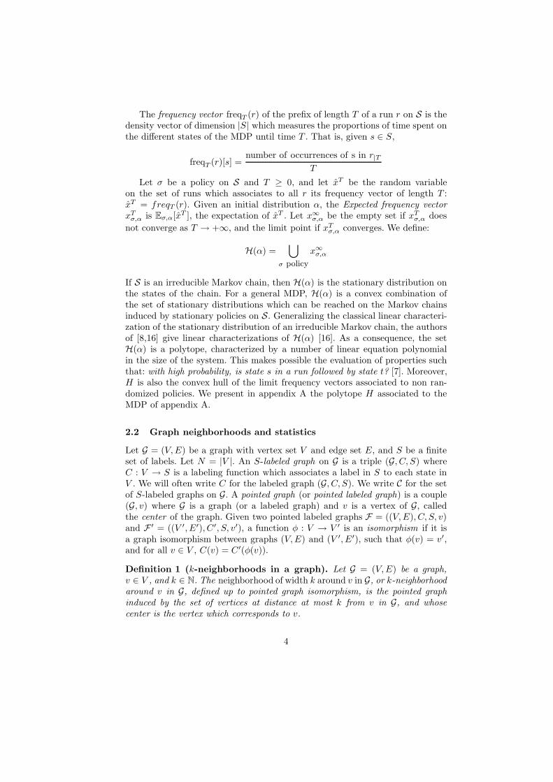
their state space is S = 0, 1. State 1 is the ”infected” state, whereas 0 is the ”non-infected” state. Non infected devices may become infected with a small probability,and infect their neighbors. The network M is a circle of N device MDPs. There is nonon-determinism in this system, since only one action is allowed.

0

1

0

0 0

1

1 1

1

Fig. 1. A circular network of MDPs.

Let r − s − tδ→ s′ describe a transition of a device in state s ∈ S with neighbors

in state r ∈ S and t ∈ S, to state s′ with probability δ. In other words, notation

r − s − tδ→ s′ holds for PD(s′|r − s − t, a) = δ. In the following, an ∗ in the notation

holds for any state. The transition function of the device MDP is given by:

∗ − 1 − ∗1

−→ 1; ∗ − 0 − 11

−→ 1;

(

0 − 0 − 0ǫ

−→ 1

0 − 0 − 01−ǫ−→ 0

This process is a Markov chain since there is no non-determinism. At each step, a

device is chosen uniformly at random among the vertices of the network, and updated.

The induced Markov chain has a state space of size 2N , and we can see that all the

configurations are reachable from the initial configuration 0 − 0 − ... − 0 with non-

zero probability. We cannot study the evolution of the chain by using explicit linear

equations on the state space if N is larger than 20. We will approximate the distri-

bution at time τ ∈ N of the proportion of infected states, using our statistical approach.

We will use shift vectors to quantify the change in the statistics of the config-urations induced by the update of the state of one device MDP in the network.Given C ∈ C, v ∈ V and a ∈ Σ, we define

∆k(C, v → s) = N · [ustatk(Cv→s) − ustatk(C)]

Given k ∈ N, a k-statistics shift vector on G is a vector ∆ ∈ [−N, N ]Nk(C)

whose components in Z sum to zero. Clearly, vectors of the type ∆k(C, v → s)are k-shift vectors. The following proposition shows that when the state of oneof the vertices of a labeled graph is changed, the variation on the k-statisticsdepends only on bounded neighborhoods around the changed vertex. It can beproven directly by counting the variations which appear on the k-statistics.

Proposition 2 ((k, φ(k))-locality). Let k ∈ N. Let φ : N → N be such thatφ(0) = 1 and φ(k) = 2 · k if k ≥ 1. Then for all C ∈ C, v ∈ V and s ∈ S wehave ∆k(C, v → s) = ∆k(N (C, v, φ(k)), v → s), i.e. for all H ∈ Nk(C) we have:

7

∆k(C, v → s)[H ] =N · [ustatk(N (C, v, φ(k))v→s))[H ] − ustatk((N (C, v, φ(k)))[H ]]

We can generalize this fact to the transition function of a network of MDPs. Inthe following, given C ∈ C, we write C′ for the random configuration distributedaccordingly to the probability distribution P (−|C, a). The following propositionis a direct consequence of proposition 2.

Proposition 3. Let M be a network of MDPs, a ∈ Σ, C ∈ C, k ∈ N, and let∆k be a k-statistics shift vector. Then:

P (ustatk(C′) = ustatk(C) + ∆k

N| C, a) =

P (ustatk(C′) = ustatk(C) + ∆k

N| ustatφ(k)(C), a)

In other words, the distribution of the k-order statistics of the configurationsafter a transition depends only on the φ(k)-th order statistics of the configurationC before the transition.

4 Structured Population Protocols with Decisions

Let G = (V, E) be a graph network, and let N = |V |. Let S be a finite set oflabels, and let C be the set of S-labeled graphs on G. Given k ∈ N, recall thatNk(C) is the set of all possible k-neighborhoods which can appear in S-labeledgraphs on the structure G. We define a Structured Population Protocol which willinduce an MDP on the set of statistics vectors. Our model generalizes classicalPopulation Protocols in two ways:

– it uses statistics on graphs neighborhoods, i.e. on a structured domain, asopposed to statistics on sets,

– decisions can be taken on states, using the same decision space Σ as theoriginal device MDPs.

A Population of statistics of order k, or k-Population, on G, is a vectorA ∈ N

Nk(C) whose components sum to N . We write Ak for the set of k-Populations. A Population can be seen as a soup of neighborhoods, i.e. a mul-tiset of neighborhoods with no structure. Given a neighborhood H in Nk(C),A[H ] is equal to the number of times the neighborhood H appears in the soupof neighborhoods A. A k-Population A induces a distribution A

Non Nk(C),

with AN

(H) = A[H ]/N . Reciprocally, an ustatk vector x = ustatk(C) inducesa k-Population A = N · x. Typically, a k-Population counts the different k-neighborhoods which appear in an S-labeled graph C on G. In that case, theprobability distribution A

N(−) is equal to ustatk(C)(−). Notice however that

there may exist k-Populations A such that for no S-labeled graph C on G we haveAN

(−) = ustatk(C)(−). As a consequence of Proposition 1, given L = |Nk(C)|,

|Ak| ≤ NL

8

As in [3], in our approach of Population Protocols, the devices, i.e. the nodesof the graph, will interact locally. The associated transition probabilities willbe given by a transition function δ. A k-Structured Population Protocols withDecisions on G is given by a transition function δ and a reconstruction functionRk. The function Rk will impose the updates to depend on the structure of theunderlying graph G.

Definition 4 (k-Structured Population Protocols with Decisions). Givenk ∈ N, a k-Structured Population Protocols with Decisions, or k-SPPD, on G, isa triple Ok = (δ, Rk, Σ) where δ : N1(C)×Σ → D(S) and Rk : Ak ×Nφ(k)(G) →D(Nφ(k)(C)).

Function δ : N1(C) × Σ → D(S) is the transition function. When |Σ| = 1,the domain of δ is N1(C) and the system is called a k-Structured PopulationProtocol, or k-SPP. In that case, our model is close to the standard model ofPopulation Protocol, [4]. Given k ≥ 0 and Hv ∈ Nφ(k)(C), δ induces a distribu-

tion δ(−|Hv, a) on the set of k-shift vectors. If ∆k is a k-shift vector, δ(∆k|Hv, a)is the probability that an update of the label of the center node v of Hv accord-ing to the transition function δ induces a change ∆k in the k-statistics. Formally,let δ(∆k|Hv, a) be defined as:

δ(∆k|Hv, a) =∑

s∈S s.t. ∆k(Hv ,v→s)=∆k

δ(N (Hv, v, 1), a)(s)

Function Rk : Ak × Nφ(k)(G) → D(Nφ(k)(C)) is a reconstruction function:given a k-Population A and Hv a φ(k)-neighborhood of the graph G, it outputsrandomly a valuation in S for the nodes of Hv. In other words, distributionRk(A, Hv)(−) assigns probabilities to the labellings of Hv.

4.1 A k-SPPD is an MDP

We associate an MDP SOkto a k-SPPD Ok as follows. The state space of SOk

isAk, the set of k-Populations, and the set of action labels is Σ. We have to definethe transition function POk

. Given a population A ∈ Ak and an action a, we firstshow how to sample a population A′ distributed according to the distributionPOk

(−|A, a). This gives a first definition for the transition function POk.

1. First, let µ = ustatφ(k)(G) be the distribution of the φ(k)-neighborhoods ofG. Sample Hv ∈ Nφ(k)(G) according to µ. This is equivalent to sampling anode in G uniformly at random and defining Hv as its φ(k)-neighborhood.

2. Sample Hv ∈ Nφ(k)(C) according to distribution Rk(A, Hv)(−). That is,sample a valuation for the nodes of Hv.

3. Sample s ∈ S according to distribution δ(a,N (Hv, v, 1))(−). That is, updatethe state of device v at the center of the neighborhood Hv.

4. Let ∆k = ∆k(Hv, v → s). ∆k represents the change in the statistics of orderk induced by the update.

5. Define A′ = A + ∆.

9

The transition function POkon SOk

can also be defined formally as follows:given ∆k a k-shift vector,

POk(A′ = A + ∆k|A, a) =

∑

H∈Nφ(k)(C), F∈Nφ(k)(G) δ(∆k|H, a) · Rk(A, F )(H) · ustatφ(k)(G)[F ]

The following proposition can be proved directly by probability conditioning.

Proposition 4. The two previous definitions of POkcoincide.

4.2 The k-SPPD associated to a network of MDPs

Let M = (G,S) be a network of MDPs, with G = (V, E) and S = (S, Σ, PD).Let S(M) = (C, Σ, P ) be the MDP associated to M. Given k ∈ N, we want todefine a k-SPPD Ok(M) = (δ, Rk, Σ′) on G such that the associated MDP SOk

mimics the transitions of S(M) on the set of k-statistics vectors.The set of actions on Ok(M) will be Σ, the same as for M. The state space of

Ok(M) will be Ak, the set of k-Populations on G, which can also be seen as theset of k-statistics of configurations on M. The transition function δ of Ok(M)will be equal to the transition function PD of the device MDPs of M. The pointis to define a relevant reconstruction function Rk. The role of the function Rk is,given a k-Population A and a φ(k)-neighborhood H ∈ Nk(G), to guess valuationsfor the nodes in H . Ideally, we would like, given C ∈ C and H ∈ Nφ(k)(G),the distributions Rk(N ·ustatk(C), H)(−) and (ustatφ(k)(C)|H)(−) to be equal.That is, the reconstruction of size φ(k) of the k-statistics of a configuration is theφ(k) statistics of the configuration. This is not possible in general, but we givean algorithm to compute the function Rk which will give good approximationson a restricted class of mixed configuration, defined in the next subsection. Thefollowing is the algorithm that we will use to define functions Rk.

Algorithm 1 (Sampling from Rk)Input: A Population A ∈ Ak, H ∈ Nφ(k)(G).

Output: H = (H, C) ∈ Nφ(k)(C) an S-valuation of the nodes of H.Method: We define C incrementally on the set of nodes of H. Until a valuationfor all the node of H is defined to the following:

1: Sample a node v uniformly at random among the nodes in H whosek-neighborhood contains unlabeled nodes, and which is at distance at most k fromthe center of H.

2: Sample K ∈ Nk(C) according to distribution ( AN|C)(−). That is,

sample K according to the distribution AN

conditioned to the partial valuationC defined so far. (See section 5.1 for a precise definition of this conditionalprobability). This corresponds to sampling labels for a neighborhood of size k inH. For all w ∈ K, define C(w) = K(w).Return H = (H, C).

Finally, given M = (G,S) the network of MDPs, using the algorithm 1 forthe construction of Rk, we have a k-SPPD Ok(M) = (δ, Rk, Σ) on G, with state

10

space Ak. In appendix B, we present the construction of the 1-SPP associatedto the contamination network of section 3.1.

Now, given a policy on the MDP M, how can we build a related policy onOk? Since the state space of M has size exponential in the state space of Ok, wecannot associate a policy on Ok to each policy on M. We will have to restrictthe class of policies that we consider on M: a policy on M must satisfy certaincompatibility properties to be transferable on Ok. A natural condition is the factthat it depends only on the k-statistics of the configurations. We call statisticalpolicies such policies on M:

Definition 5 (Statistical Policies). A policy σ on M is k-statistical if:

∀C, C′ ∈ C, ustatk(C) = ustatk(C′) ⇒ σ(C) = σ(C′)

Let SRk(M) be the set of k-Statistical and Randomized policies. For in-stance, a policy which takes its decisions according to the 0-statistic of the con-figurations, i.e. according to the proportions of the different states among thedevices, is k-statistical for all k ∈ N. A policy σ ∈ SRk(M) induces trivially apolicy σ on Ok, since σ can be defined on the set of ustatk vectors, hence on Ak.

5 Approximations on Networks of MDPs.

Let M be a network of MDPs as before, with state space C and transitionfunction P , and let Ok be the associated k-SPPD, with state space Ak andtransition function POk

. In this section we show that we can bound the differencein the evolutions of the statistics of the real process induced by M, and theevolution of the approximation process induced by Ok. More precisely, we showthat we can define a notion of mixed configurations, quantified by a mixingparameter, such that the reconstruction function Rk defined by algorithm 1 onthe Population Protocol approximates M.

5.1 Mixed configurations

A partially labeled graph is a graph such that labels are associated only to asubset of nodes. In particular, a graph H = (V, E) can be seen as a partiallylabeled graph, where no valuation is defined for any node. We write Nk(Cp)for the set of k-neighborhoods of partially labeled graphs on G. Given F, F ′

two partially labeled graphs on the same domain G, F and F ′ are said to becompatible if there exists no node of G to which F and F ′ assign different labels.Given CH a partially labeled graph on a graph H , we define L(CH) as the setof labeled graphs on H compatible with CH . We need to condition probabilitydistributions by a structure: given a distribution µ on Nk(C), given H ∈ Nk(G)and given CH a partially labeled graph on H such that µ(L(CH )) > 0 , thedistribution (µ|CH)(−) on Nk(C) is defined as follows: for all K ∈ Nk(C),

(µ|CH)(K) = 0 if K 6∈ L(CH) and else (µ|CH)(K) =µ(K)

µ(L(CH))

11

We now want to quantify the quality of the reconstruction function Rk. Aswe said before, ideally, given a configuration C ∈ C and H ∈ Nφ(k)(G), thedistributions Rk(N ·ustatk(C), H)(−) and (ustatφ(k)(C)|H)(−) should be equal.However, this is not possible in general, since there may exist configurationsC, C′ ∈ C such that ustatk(C) = ustatk(C′) but ustatφ(k)(C) 6= ustatφ(k)(C

′).We present a class of configurations for which there exist good reconstructionfunctions, i.e. functions Rk such that the distributions Rk(N · ustatk(C), H)(−)and (ustatφ(k)(C)|H)(−) are close. Such configurations can be seen as ”mixed”configurations, and we define a mixing coefficient.

Let C ∈ C, let v be a node in C and let H = N (C, v, k). Let K be apartial labeling of N (G, v, φ(k)) such that the partial labeling KH induced byK on N (G, v, k) is compatible with H . Let PC be the probability distributionustatk(C)(−). We define the following conditional probabilities: PC [H |H ∩K] isthe probability, among the k-neighborhoods of C, of the neighborhood H , giventhe partial valuation KH is given. PC [H |K] is the probability, among the φ(k)-neighborhoods of C, of the neighborhood which contains H around its center,given the partial valuation K is given. Formally:

PC [H |H ∩ K] =|u ∈ V s.t. N (C, u, k) ≃ H|

|u ∈ V s.t. N (C, u, k) ∈ L(KH)|

PC [H |K] =|u ∈ V s.t. N (C, u, k) ≃ H ∧ N (C, u, φ(k)) ∈ L(K)|

|u ∈ V s.t. N (C, u, φ(k)) ∈ L(K)|

If K is not compatible with C, let PC [H |H ∩ K] = PC [H |K] = 0.

Definition 6 (Mixing coefficient ǫk). Let C ∈ C be a configuration. Thek-mixing coefficient of C is defined as:

ǫk(C) = MaxH=N (C,u,k), K∈Nφ(k)(Cp)|PC [H |H ∩ K] − PC [H |K]|

Intuitively, ǫk(C) is small if the distribution of the k-neighborhoods does notdepend on their environment. We say that C is well mixed if ǫk(C) is small. Thefollowing proposition, proved in appendix D, shows that if configuration C iswell mixed, the function Rk defined by the algorithm 1 is a good reconstructionfunction. We measure the distance between the distributions using the ‖ ‖∞-norm: given v ∈ R

n, ‖v‖∞ = maxi∈[1;n]|vi|. As a consequence, if C is wellmixed, we can find a good approximation of ustatφ(k)(C) from ustatk(C). Thisis exactly what the function Rk is supposed to do. In appendix C we present anexample of statistics for the circular network.

Proposition 5. Let C ∈ C be a configuration, and let Rk be defined by algorithm1. Then for all H ∈ Nφ(k)(G) we have:

‖Rk(N · ustatk(C), H)(−) − (ustatφ(k)(C)|H)(−)‖∞ ≤ ǫk(C)

We now use the mixing coefficient to give bounds on approximation of thebehavior of networks of MDPs by our k-SPPDs. In [13], the authors approximate

12

the short term evolution of large Markov chains by using a “sliding windows”approach. As in [13], we try to bound the deviation between our approximationand the real process as time goes on. Given C ∈ C and a ∈ Σ, we write C′ for therandom configuration induced by the probability distribution P (−|C, a). GivenC ∈ C and A = N · ustatk(C), define the distributions µk

C,a and νkA,a on Ak as

follows: given A′ ∈ Ak, let:

µkC,a(A′) = P (N · ustatk(C′) = A′ | C, a), and νk

A,a(A′) = POk

(A′ | A, a)

In other words, µkC,a(−) is the distribution of the k-statistics of configurations

after a transition from the configuration C, on the network of MDPs M. On theother hand, νk

A,a(−) is the distribution of the k-statistics after a transition fromthe population N ·ustatk(C), on Ok. The following theorem measures the qualityof the approximation of the network of MDPs by the k-SPPD, on the set of k-statistics. It is proved in appendix D.

Theorem 1. ‖µkC,a − νk

A,a‖∞ ≤ ‖ustatk(C)(−) −A

N(−)‖∞ + ǫk(C)

5.2 Approximation for Markov Chains: The Evaluation Problem.

For this subsection, we assume that the process induced on the set of con-figurations by M is a Markov chain. This is the case when there is no non-determinism on M, or when a stationary policy has been fixed and resolves thenon-determinism of M. Let Xnn∈N be the Markov chain induced on C, givenan initial configuration C0 ∈ C is fixed. Let Ok be the associated k-SPP on statespace Ak, and let Uk

nn∈N be the Markov chain induced by Ok on Ak.We compare the evolutions of the distributions on the set of statistics vectors

induced by ustatk(Xn)n∈N and Uknn∈N. The question is the following: in case

of convergence of Xn to a configuration C ∈ C, does the approximate process Ukn

converges also to a limit close to N · ustatk(C)? Moreover, in case of multiplestationary configurations for Xn, does process Uk

n converge to close limits withclose probabilities?

We show that the answer is positive in the context of the circular contami-nation graph. However, a consequence of the lower bound on the computationalcomplexity of the reachability problem for Cellular Automata is that the thereachability problem for network of MDPs is PSPACE complete. This can beproved by a slight generalization of theorem 4.2 of [5] to the context of asyn-chronous Cellular Automata. As a consequence, the evaluation problem for Xn

and ustatk(Xn) are computationally intractable, hence we cannot expect theapproximation Uk

n to always match closely the process N · ustatk(Xn).

Theorem 2. If configuration C ∈ C is a fixpoint for the chain Xnn∈N, i.e. aconfiguration such that P[Xn+1 = C′|Xn = C] = 1 if C′ = C and 0 if C′ 6= C,then for all k ≥ 1, N · ustatk(C) ∈ Ak is a fixpoint for the chain Uk

nn∈N.

Proof. If C is a fixpoint, all neighborhoods in N1(C) which appear in C arestable for the transition function δ. All the neighborhoods of N1(C) centered in

13

the neighborhoods that we sample from the distributions Rk(N · ustatk(C), H)are also stable, i.e. P[Uk

n+1 = Ukn |U

kn = N · ustatk(C)] = 1, hence N · ustatk(C)

is a fixpoint for the chain Uknn∈N.

In appendix E.1, show that the converse of theorem 2 does not hold: theremay exist fixpoints for the chain Uk

nn∈N which do not correspond to the ustatkvector of any configuration. We prove that in the contamination model, suchfixpoints of Uk

nn∈N are not reachable from an initial state which correspondsto the ustatk vector of a configuration. In appendix E.2, we prove that theorem2 does not hold for k = 0: the transition function of the approximation processU0

nn∈N is too weak since it does not consider overlappings of neighborhoods.

5.3 Approximations for Markov Decision Processes.

Now, we extend our approach to networks of MDPs with non-determinism. GivenM, the associated polytope H (see section 2.1) is a subset of R

C . The k-SPPDOk associated to M is also an MDP, and its polytope lies in R

Ak . How can werelate these two polytopes?

We consider the set of the limit points associated to stationary statisticspolicies on M, and we prove that it is also a polytope. We obtain a natural ap-proximation of Hk

stat(M) by the polytope H(Ok) associated to all the stationarypolicies on Ok.

Theorem 3. The set Hkstat(M) = N · ustatk(x∞

σ,α) | σ ∈ SRk is a polytope

of RAk , with a number of extremal points polynomial in N .

Proof. First, notice that a convex combination of k-statistical policy is clearlya statistical policy. Thus, Hk

stat(M) is convex. Next, any statistical policy isa convex combination of ”deterministic” statistical policies which assign Diracdistribution to statistic vectors of configurations. (i.e. policies σ such that, givenA ∈ Ak, σ(A) ∈ Σ). This proves that Hk

stat(M) is a polytope, and it is theconvex hull of the limit frequency vectors associated to deterministic statisticalpolicies. We can conclude using the fact that since there exists only a polynomialnumber of ustatk vectors of configurations in Ak, there exists only a polynomialnumber of ”deterministic” statistical policies, hence of extremal points of thepolytope.

6 Conclusion

We have studied how to approximate the evolution of large probabilistic networksof MDPs. Given a network M of N device MDPs, we defined a k-StructuredPopulation Protocol with Decisions Ok, which is also an MDP, whose statesare statistics vectors. From an exponential number of configurations, we obtaina polynomial number of statistics. This allows the use of standard evaluationmethods on the approximation system, and we gave a sufficient condition, usinga mixing parameter ǫk, to guarantee a good approximation. If we discretize the

14

statistics vectors up to a coefficient γ, the size of the set of configurations of theapproximation process becomes independent of N : it depends only on δ, k, andthe degree of the underlying graph. In appendix F, we present the values of thesizes of the state spaces of the real and the approximation processes for variousparameters, underlying the efficiency of the discretization model.

References

1. Hons R. Agapie, A. and H. Muhlenbein. Markov Chain Analysis for One-Dimensional Asynchronous Cellular Automata. Methodology and Computing inApplied Probability, 6(2):181–201, 2004.

2. D. Angluin, J. Aspnes, M. Chan, M.J. Fischer, H. Jiang, and R. Peralta. Stablycomputable properties of network graphs. Lecture Notes in Computer Science,3560:63–74, 2005.

3. D. Angluin, J. Aspnes, Z. Diamadi, M.J. Fischer, and R. Peralta. Computation innetworks of passively mobile finite-state sensors. Distributed Computing, 18(4):235–253, 2006.

4. J. Aspnes and E. Ruppert. An introduction to population protocols. Bulletin ofthe EATCS, 93:106–125, 2007.

5. C.L. Barrett, H.B. Hunt, M.V. Marathe, SS Ravi, D.J. Rosenkrantz, and R.E.Stearns. Complexity of reachability problems for finite discrete dynamical systems.Journal of Computer and System Sciences, 72(8):1317–1345, 2006.

6. C. Courcoubetis and M. Yannakakis. The complexity of probabilistic verification.JACM, 42(4):857–907, 1995.

7. M. de Rougemont and M. Tracol. Statistical analysis for probabilistic processes.In IEEE Logic in Computer Science(2009), pages 299–308.

8. C. Derman. Finite State Markovian Decision Processes. Academic Press, Inc.Orlando, FL, USA, 1970.

9. R. Durrett. Stochastic spatial models. Siam Review, 41(4):677–718, 1999.10. J. Esparza. Decidability and complexity of Petri net problems-an introduction.

Lecture Notes in Computer Science, pages 374–385, 1998.11. E. Fischer, F. Magniez, and M. de Rougemont. Approximate satisfiability and

equivalence. In IEEE Logic in Computer Science, pages 421–430. Citeseer, 2006.12. I. Harvey and T. Bossomaier. Time out of joint: Attractors in asynchronous random

boolean networks. In Proceedings of the Fourth European Conference on ArtificialLife, pages 67–75, 1997.

13. T.A. Henzinger, M. Mateescu, and V. Wolf. Sliding window abstraction for infiniteMarkov chains. In Proc. CAV, volume 5643, pages 337–352. Springer.

14. JM Kahn, RH Katz, and KSJ Pister. Next century challenges: mobile network-ing for Smart Dust. In Proceedings of the 5th annual ACM/IEEE internationalconference on Mobile computing and networking, pages 271–278. ACM, 1999.

15. M. Kwiatkowska, G. Norman, and D. Parker. Probabilistic symbolic model check-ing with prism: A hybrid approach. In Proc. TACAS. Springer Verlag, 2002.

16. M.L. Puterman. Markov Decision Processes: Discrete Stochastic Dynamic Pro-gramming. John Wiley & Sons, Inc. New York, NY, USA, 1994.

17. K. Sutner. On the computational complexity of finite cellular automata. Journalof Computer and System Sciences, 50(1):87–97, 1995.

18. M.Y. Vardi. Automatic verification of probabilistic concurrent finite state pro-grams. In FOCS 1984, pages 327–338, 1985.

19. S. Wolfram. Cellular automata. Los Alamos Science, 9(2-21):42, 1983.

15

A A Simple MDP and its polytope

Let S = s, t, u, w, Σ = a, b, c and the transitions given by the Figure 2.Nodes s, u are deterministic, node t, w are non deterministic, node t is alsoprobabilistic: P (s|b, t) = .5 and P (u|b, t) = .5. A policy specifies the decision aor b in state t, and the decisions b or c in state w. If the original distributionα specifies the state s with probability 1, a possible run is s, t, u, w, u. The 4stationary strategies σ1, σ2, σ3, σ4 are: σ1(t) = a; σ1(w) = b, σ2(t) = a; σ2(w) =c, σ3(t) = b; σ3(w) = b, and σ4(t) = b; σ4(w) = c. Let us now construct H(S),

a

aa

b: .5

b: .5b

cs

t u

w

Fig. 2. An MDP with 4 states: nodes t,w are non deterministic, i.e. the transitions arespecified by a policy σ.

the polytope of order 1 for the MDP of Figure 1. We consider the frequencyvectors, which are distributions on s, t, u, w. By simple calculations on theMarkov chains, we get the following limit frequency vectors associated to thestationary strategies σ1, σ2, σ3, σ4: y1 = (0; 0; 1/2; 1/2), y2 = (1/4; 1/4; 1/4; 1/4),y3 = (2/6; 2/6; 1/6; 1/6), and y4 = (0; 0; 1/2; 1/2).

The polytope H(S) is represented partially in Figure 3, using a projection ontwo dimension: the interpretation is that the limit frequency vector associatedto any policy lies in the polytope. We can then decide given a run and itsfrequency vector y of order k if there is a policy σ which will witness runs ε-close to y, using the Edit distance with moves as a distance between runs seenas sequences of letters [7] when k = 1

ε. In Figure 3, y is the frequency vector of

some run, which is at distance d from H(S). The closest point y′ is the limitfrequency vector of the randomized policy σ′ = 1

3 .σ1 + 23 .σ2, i.e. σ′(t) = a and

σ′(w) = b : 13 , σ′(w) = b : 2

3 .

distance

y1

y2

y3

y

y’

Fig. 3. The polytope H(S) for the MDP of Figure 1.

16

B The 1-SPP associated to the contamination network

Let O1 = (δ, R1, Σ) be the 1-SPP associated to M, the circular contaminationnetwork of section 3.1. The state space of O1 is A1, the set of 1-Populations. Weknow that:

|A1| ≤ N |N1(C)|

Since N1(C) = b1− b2 − b3 | b1, b2, b3 ∈ 0, 1 and since the neighborhoods aretaken up to labeled graph isomorphism, we get |A1| ≤ N6, which allows large Nin practice. The set of labels Σ for Oi is the same as for M, hence it is reducedto only one label.

We present an example of a sampling from the function R1, i.e. we presentan execution of algorithm 1 on an input A, H . We have k = 1, hence φ(k) = 2.We have Nφ(1)(G) = · − · − · − · − ·, hence H = · − · − · − · − ·. Suppose forinstance that

AN

= (000 : 0.10; 001 : 0.1; 010 : 0.10; 011 : 0.10;100 : 0.15; 101 : 0.16; 110 : 0.40; 111 : 0.24)

We want to output H , a valuation for the five nodes of H . We use the methodof the algorithm 1.

– 1: we sample a node v uniformly at random among the nodes in H , atdistance at most 1 from the center of H . Suppose for instance that we samplethe center node.

– 2: we sample K ∈ Nk(C) according to distribution AN

conditioned to thepartial labeling C defined so far. Since no partial labeling have been definedso far, this is equivalent to sampling K ∈ Nk(C) according to A

N. Suppose

for instance that we sample K = 1−0−0. For all w ∈ K, let C(w) = K(w).– So far, we have defined the partial valuation · − 1 − 0 − 0 − · on H .– 1bis: we sample a node v uniformly at random among the nodes in H whose

k-neighborhood contains unlabeled nodes, and which is at distance at most1 from the center of H . Suppose for instance that we sample the node onthe right of the center.

– 2bis: we sample K ∈ Nk(C) according to distribution AN

conditioned to thepartial labeling C defined so far. We have N (v, C, 1) = 0 − 0 − ·, hence, bydefinition of the probability conditioning we sample K = a1−a2−a3 ∈ N1(C)with probability 0 if a1 − a2 6= 0 − 0, and else with probability

A

N(K|0 − 0 − ·) =

A[a1 − a2 − a3]

A[0 − 0 − ∗]

For instance, if K = 0−0−1, since A[0−0−1] = 0.1 and A[0−0−0]+A[0−

0 − 1] = 0.1 + 0.1 = 0.2, the probability to sample K is0.1

0.2= 1

2 . Suppose

we sample indeed 0 − 0 − 1.– So far, we have defined the partial valuation · − 1 − 0 − 0 − 1 on H .– In another execution of steps 1 and 2, we may finally get the valuation

H = 0 − 1 − 0 − 0 − 1 on H .

17

C Probability conditioning

Consider the Circular Network of the contamination model, presented in section3.1. Let k = 1, hence φ(k) = 2. In the following, we write · to denote a node ofa partially labeled graph whose label is not defined. As before, a ∗ may hold forany label. Hence, for instance, we write ·− ...− · for a linear graph with n nodeswith no valuation defined, and a1 − ·− a3 − · is the linear graph with four nodeswith two of them labeled a1 and a3. In the contamination model, we have:

N1(G) = · − · − ·; and N2(G) = · − · − · − · − ·

In fact, we have

N1(Cp) = b1 − b2 − b3 | b1, b2, b3 ∈ 0, 1, ·and N2(Cp) = b1 − b2 − b3 − b4 − b5 | b1, ...b4 ∈ 0, 1, ·

To illustrate our notion of conditional probabilities, we consider two types ofneighborhoods.

First, let:

K = · − · − · − · − 1, and H = a2 − a3 − a4, with a2, a3, a4 ∈ 0, 1

We have K ∈ Nφ(k)(Cp), and H ∈ L(N (K, v, k)). By definition, given a configu-ration C ∈ C, we have:

PC [H |H ∩ K] =|u ∈ V s.t. N (C, u, k) ≃ H|

|u ∈ V s.t. N (C, u, k) ∈ L(KH)|

Since K = · − · − · − · − 1 and the center of K is the third node, we haveKH = ·− ·− ·, hence any configuration in N1(C) is an extension of KH . In otherwords, L(KH) = N1(C). Hence, we get

PC [H |H ∩ K] =|u ∈ V s.t. N (C, u, k) ≃ H|

|V |= ustatk(C)[H ]

This means that the conditional probability of H conditioned to H ∩ K is infact the probability of H to appear as neighborhood in C. This is coherent withthe intuition that H ∩ K should not interfere with the probability of K, sincethe partial valuation K forces no valuations for nodes in H . With analogouscalculations, we have:

PC [H |K] =#C ∗ −a2 − a3 − a4 − 1

#C ∗ − ∗ − ∗ − ∗ −1

Where #C ∗ −a2 − a3 − a4 − 1 is the number of neighborhoods of width 2 in Cwhich are of the form ∗−a2−a3−a4−1, where ∗ = 0 or 1, and #C ∗−∗−∗−∗−1is the number of neighborhoods of the form ∗−∗−∗−∗−1 in C. In other words,#C(H) = N · ustatk(C)[H ].

18

Hence, |PC [H |H∩K]−PC [H |K]| is small if the proportion of neighborhoodsa2a3a4 among the 1-neighborhoods of C is close to the proportion of the neigh-borhoods of the form ∗ − a2 − a3 − a4 − 1 among the 2-neighborhoods of C ofthe form ∗ − ∗ − ∗ − ∗ − 1. This is coherent with the intuition of a ”mixingconfiguration”: the probability to have a 1 on the right does not depend on thecenter of the neighborhood.

Second, let K ′ ∈ Nφ(k)(Cp) be · − · − · − 1 − 1. Then, given a configurationC ∈ C, we have PC [H |H ∩ K ′] = 0 if a4 6= 1, and else

PC [H |H ∩ K ′] =#Ca2 − a3 − 1

#C ∗ − ∗ −1

Which is different from ustatk(C)[H ] in general. Also, we have:

PC [H |K ′] =#C ∗ −a2 − a3 − 1 − 1

#C ∗ − ∗ − ∗ −1 − 1

The typical example of a perfectly mixed configuration, i.e. for which ǫ1(C) =0, for 1-statistics in the contamination model network, is a configuration wherethere is a majority of 0 states, except some 1’s which are repartited such thatno couple of 1’s are separated by less than two 0 states.

D Proofs for section 5

Proposition 5. Let C ∈ C be a configuration, and let Rk be defined by algorithm1. Then for all H ∈ Nφ(k)(G) we have:

‖Rk(N · ustatk(C), H)(−) − (ustatφ(k)(C)|H)(−)‖∞ ≤ ǫk(C)

Proof. Let A = ustatk(C). We write µ for the distribution Rk(N ·ustatk(C), H)(−),and ν for the distribution (ustatφ(k)(C)|H)(−), both on Nφ(k)(C). Let H ∈Nφ(k)(C).

First, if H 6∈ L(H), then by definition of Rk we have Rk(N ·ustatk(C), H)(H) =0, and by definition of the conditional probability (ustatφ(k)(C)|H)(−), we have

(ustatφ(k)(C)|H)(H) = 0.

Let H ∈ L(H). For this proof, we fix an input N · ustatk(C), H for thealgorithm 1. A step of the algorithm 1 is an execution of the points 1 and 2. Thealgorithm 1 is randomized, and always stops after at most |H | steps. Let Γ bethe set of possible executions on input N · ustatk(C), H , which is a finite set.Given γ ∈ Γ , let iγ be the number of steps of the execution. Given γ ∈ Γ andj ∈ [1; iγ ], let Hγ

j be the partially labeled graph defined on H after j iterations,and let Kj ∈ Nk(C) be the neighborhood which is sampled at the point 2 of thej-th step. We define H0 = H .

Let Ω be the set of finite sequence H0, ..., Hi of partially labeled graph on Hsuch that H0 = H , Hi = H, and for all j ∈ [0; i − 1], Hj+1 is an extension ofHj (i.e. Hj+1 defines more labels for nodes that Hj , and the labels of Hj+1 arecompatible with the labels of Hj).

19

Given j ∈ N, let Pj be the distribution of probability on executions associatedto the algorithm after j steps, on input N · ustatk(C), H . For instance, givenKj ∈ Nk(C), Pj [Kj |Hj ] is the probability to sample Kj at point 2 of the secondstep of the algorithm, given partially labeled graph Hj has been defined so far.Then, by conditional probability, we have:

Rk(N · ustatk(C), H)(H) =∑

H0,...,Hi∈Ω

i−1∏

j=0

Pj[Hj+1|Hj ]

Now, given H0, ..., Hi ∈ Ω and j ∈ [0; i − 1],

Pj [Hj+1|Hj ] =∑

Kj∈Nk(C)

Pj[Hj+1|Hj ∧ Kj] · Pj [Kj |Hj ]

Given Kj ∈ Nk(C), by the definition of the algorithm, we have

Pj[Kj |Hj ] = (ustatk(C)(−)|Hj ∩ Kj)(Kj)

That is,

Pj[Kj |Hj ] = PC [Kj|Hj ∩ Kj] (1)

Indeed, the sample in the point 2 of the algorithm is done conditionally to theneighborhoods of width k.

On the other hand, since if H0, ..., Hi ∈ Ω all the Hj in H0, ..., Hi are com-patible with H , we have:

(ustatφ(k)(C)|H)(H) =∑

H0,...,Hi∈Ω

i−1∏

j=0

PC(Hj+1|Hj)

Now,

PC(Hj+1|Hj) =∑

Kj∈Nk(C)

PC [Hj+1|Hj ∧ Kj] · PC [Kj |Hj ]

We have PC [Hj+1|Hj ∧ Kj ] = Pj [Hj+1|Hj ∧ Kj ]. All we have to do is tobound

|PC [Kj |Hj ] − Pj [Kj |Hj ]|

But, by equation 1,

|PC [Kj|Hj ] − Pj [Kj|Hj ]| = |PC [Kj |Hj ] − PC [Kj|Hj ∩ Kj]| ≤ ǫk(C)

Which gives the result.

Theorem 1. ‖µkC,a − νk

A,a‖∞ ≤ ‖ustatk(C)(−) −A

N(−)‖∞ + ǫk(C)

20

Proof. This is a consequence of the proposition 5. By (k, φ(k)) locality, give ak-shift vector ∆k, we have:

µkC,a(A+∆k) =

∑

H∈Nφ(k), H∈L(H)

ustatφ(k)(G)[H ]·(ustatφ(k)(C)(−)|H)[H ]·δ(∆k|H, a)

On the other hand, if A = ustatk(C), we have:

νkA,a(A + ∆k) = POk

(A + ∆k|A, a) =∑

H∈Nφ(k), H∈L(H)

Rk(A, H)(H) · δ(∆k|H, a)

This proves the result since by proposition 5,

‖ustatφ(k)(G)[H ] · (ustatφ(k)(C)(−)|H)[−] − Rk(A, H)(H)‖∞ ≤ ǫk(C)

E Remarks on Theorem 2.

E.1 The converse of theorem 2 does not hold

We consider the order 1 statistics of the circle contamination model of appendixC. Given A ∈ A1 and a, b ∈ 0, 1, we write A[∗−a−b] for A[0−a−b]+A[1−a−b]:the symbol ∗ holds for a projection on the associated component. Then, it isnot difficult to see that all the fixpoints of the chain U1

nn∈N are exactly theA ∈ A1 such that A[∗−0−∗] = 0. Indeed, if the state of the center device of anyneighborhood of width 1 is one, then there is no change when we make an update,and A is a fixpoint. However, there exists A ∈ A1 such that A[∗−0−∗] = 0 andwhich corresponds to no ustat1 of configuration in C.

We prove that these fixpoint are in fact unreachable from any initial config-uration which corresponds to the ustat1 vector of a configuration. We prove theresult by induction: for all n ∈ N we have U1

n[∗−0−∗] > 0, or U1n[1−1−1] = 1.

In fact, we prove the following: for all n ∈ N, U1n[∗ − 0 − ∗] = U1

n[∗ − ∗ − 0] =U1

n[0 − ∗ − ∗].

– The base case is U10 = N ·ustat1(C0), where C0 the initial configuration is in

C. Then the results follows directly from the fact that the underlying graphis a circle.

– Suppose the result true for U1n, n ∈ N. Then we remark that the change in

the statistics of order two that the transition makes respects the property:for instance, if algorithm 1 guesses a neighborhood y = [0 − 1 − 0 − 0 − 1]and the state of the center device is updated to 1, then the shift vector ∆ issuch that ∆[∗ − 0 − ∗] = −1 = ∆[∗ − ∗ − 0] = ∆[0 − ∗ − ∗].

Now, if for all n ∈ N we have U1n[∗ − 0 − ∗] = U1

n[∗ − ∗ − 0] = U2n[0 − ∗ − ∗],

then U1n[∗ − 0 − ∗] = 0 implies U1

n[1 − 1 − 1] = N , i.e. A is the ustat1 vector ofthe stationary configuration for Xnn∈N where all devices are in state 1.

21

E.2 Theorem 2 does not hold for k = 0

Consider a circular network analogous to the contamination model, where thetransition function of the device MDPs has been changed to:

1 − 0 − 11

−→ 0; 1 − 1 − ∗1

−→ 1;

0 − 1 − 1ǫ

−→ 0

0 − 1 − 11−ǫ−→ 1

Suppose that N the number of device MDPs in the circular network is even,and let C = ...0 − 1 − 0 − 1 − 0 − 1... be the circular configuration whichis an alternating sequence of 0’s and 1’s. Then by definition of the transitionfunction of the device MDPs, C is a fixpoint of the process induced on the setof configuration by the network of MDPs. Now, let O0 be the 0-SPP associatedto the network of MDPs, and let A = N · ustat0(C) ∈ A0 be the populationassociated to C. Notice that we have

R0(A, · − · − ·)(011) > 0

Indeed, we have R0(A, · − · − ·)(011) ≥ AN

[0] ∗ AN

[1] ∗ AN

[1]. As a consequence,since δ(0 − 1 − 1, a)(1) > 0 and δ(0 − 1 − 1, a)(0) > 0, we have:

PO0(A′[1] = A[1] + 1|A, a) > 0 and PO0(A

′[1] = A[1]|A, a) > 0

or

PO0(A′[1] = A[1] − 1|A, a) > 0 and PO0(A

′[1] = A[1]|A, a) > 0

In both cases, this proves that A is not a fixpoint for the chain U0n.

F Practical bounds on the Structured Population

Protocols

The goal is to apply our approach to the study of real systems, such as largesensor networks. In the following w give bounds on the sizes of the state spaces ofStructured Population Protocols associated to various classes of networks, andcorresponding to statistics of order 0,1 or 2. We see that the size of the systemsare reasonable for statistics of order 0 or 1, 1 being the most interesting case.Using discretization, we see that we can easily consider networks with up to10000 nodes.

In the following table we consider various networks of MDPs on device MDPsfor which |S| = 2. We present the size of the state spaces of these networks, andthe sizes of the associated k-SPPDs. We consider two different parameters forthe networks: d is the degree of the underlying graphs (for instance 2 in the cir-cular contamination model), and N is the number of nodes of the graph. In thetable, # network is the number of configurations on the network of MDPs, andgiven k ∈ N, # k-SPPD is the size of the of the associated k-SPPDs. We have#k − SPPD ∼ N |Nk(C)|, hence we have to compute the values of the |Nk(C),

22

which can be done easily since we consider small graphs, with k ∈ 0, 1, 2. Re-mark that for all d, we have |N0(C)| = 2, since the 0-neighborhoods correspondto the node of the graphs and |Σ| = 2. Hence for all d, #0 − SPPD = N2. Anetwork of N device MDPs has size #network ∼ 2N . Finally, the size of the 5%discretized k-SPPD has size less than 20|N2(C)|.

N d |N1(C)| |N2(C)| # network # 0-SPPD # 1-SPPD # 2-SPPD # 2-SPPD 5%

10 2 6 20 1024 100 ≤ 1024 ≤ 1024 ≤ 102420 2 6 ∼ 106 400 ≤ 106 ≤ 106 ≤ 106

1000 2 6 ≥ 1050 106 ∼ 1020 ∼ 108 ∼ 108

10000 2 6 ≥ 1050 1010 ∼ 1024 ≥ 1050 ∼ 108

10 3 8 109 1024 100 ≤ 1024 ≤ 1024 ≤ 102420 3 8 109 ∼ 106 400 ≤ 106 ≤ 106 ≤ 106

1000 3 8 109 ≥ 1050 106 ∼ 1020 ≥ 1050 ∼ 1010

10000 3 8 109 ≥ 1050 1010 ∼ 1032 ≥ 1050 ∼ 1010

10 4 10 ≥ 1050 1024 100 ≤ 1024 ≤ 1024 ≤ 102420 4 10 ≥ 1050 ∼ 106 400 ≤ 106 ≤ 106 ≤ 106

1000 4 10 ≥ 1050 ≥ 1050 106 ∼ 1030 ≥ 1050 ∼ 1013

10000 4 10 ≥ 1050 ≥ 1050 1010 ∼ 1040 ≥ 1050 ∼ 1013

23