PROBABILISTIC RELIABILITY ENGINEERING - …gnedenko-forum.org/library/Ushakov/Probabilistic...
454
PROBABILISTIC RELIABILITY ENGINEERING Probabilistic Reliability Engineering, Boris Gnedenko and Igor Ushakov
Transcript of PROBABILISTIC RELIABILITY ENGINEERING - …gnedenko-forum.org/library/Ushakov/Probabilistic...

PROBABILISTIC RELIABILITY ENGINEERING
Probabilistic Reliability Engineering, Boris Gnedenko and Igor Ushakov
PROBABILISTIC RELIABILITY ENGINEERING
BORIS GNEDENKO Moscow State University and SOTAS, Inc.
IGOR USHAKOV SOTAS, Inc. and George Washington University
Edited by JAMES FALK George Washington University
A Wiley-lnterscience Publication
JOHN WILEY & SONS, INC. New York / Chichester / Brisbane / Toronto / Singapore

This text is printed on acid-free paper.
Copyright © 1995 by John Wiley & Sons, Inc.
All rights reserved. Published simultaneously in Canada.
Reproduction or translation of any part of this work beyond that permitted by Section 107 or 108 of the 1976 United States Copyright Act without the permission of the copyright owner is unlawful. Requests for permission or further information should be addressed to the Permissions Department, John Wiley & Sons, Inc.
This publication is designed to provide accurate and authoritative information in regard to the subject matter covered. It is sold with the understanding that the publisher is not engaged in rendering professional services. If legal accounting, medical, psychological, or any other expert assistance is required, the services of a competent professional person should be sought.
ISBN-0-471-30502-2
1 0 9 8 7 6 5 4 3 2 1

v
CONTENTS
Preface xv
Introduction xvii
1 Fundamentals 1 1.1 Discrete Distributions Related to Reliability / 1
1.1.1 Bernoulli Distribution / 1 1.1.2 Geometric Distribution / 2 1.1.3 Binomial Distribution / 5 1.1.4 Negative Binomial Distribution / 6 1.1.5 Poisson Distribution / 8
1.2 Continuous Distributions Related to Reliability / 10 1.2.1 Exponential Distribution / 10 1.2.2 Erlang Distribution / 14 1.2.3 Normal Distribution / 15 1.2.4 Truncated Normal Distribution / 19 1.2.5 Weibull-Gnedenko Distribution / 19 1.2.6 Lognormal Distribution / 22 1.2.7 Uniform Distribution / 24
1.3 Summation of Random Variables / 25 1.3.1 Sum of a Fixed Number of Random
Variables / 25

Xii CONTENTS
1.3.2 Central Limit Theorem / 28 1.3.3 Poisson Theorem / 30 1.3.4 Random Number of Terms in the Sum / 31 1.3.5 Asymptotic Distribution of the Sum of a Random
Number of Random Variables / 32 1.4 Relationships Among Distributions / 34
1.4.1 Some Relationships Between Binomial and Normal Distributions / 34
1.4.2 Some Relationships Between Poisson and Binomial Distributions / 35
1.4.3 Some Relationships Between Erlang and Normal Distributions / 36
1.4.4 Some Relationships Between Erlang and Poisson Distributions / 36
1.4.5 Some Relationships Between Poisson and Normal Distributions / 37
1.4.6 Some Relationships Between Geometric and Exponential Distributions / 38
1.4.7 Some Relationships Between Negative Binomial and Binomial Distributions / 38
1.4.8 Some Relationships Between Negative Binomial and Erlang Distributions / 39
i .4.9 Approximation with the Gram-Charlie Distribution / 39
1.5 Stochastic Processes / 42 1.5.1 Poisson Process / 42 1.5.2 Introduction to Recurrent Point Processes / 47 1.5.3 Thinning of a Point Process / 53 1.5.4 Superposition of Point Processes / 54
1.6 Birth and Death Process / 56 1.6.1 Model Description / 56 1.6.2 Stationary Probabilities / 58
1.6.3 Stationary Mean Time of Being in a Subset / 60 1.6.4 Probability of Being in a Given Subset / 61 1.6.5 Mean Time of Staying in a Given Subset / 64 1.6.6 Stationary Probability of Being in a Given
Subset / 65 1.6.7 Death Process / 65 Conclusion / 68 References / 69
CONTENTS Xijj
Appendix: Auxiliary Tools / 70 l.A.l Generating Functions / 70 1.A.2 Laplace-Stieltjes Transformation / 71 1.A.3 Generalized Generating Sequences / 74 Exercises / 79 Solutions / 81
2 Reliability Indexes 86 2.1 Unrepairable Systems / 87
2.1.1 Mean Time to Failure / 87 2.1.2 Probability of a Failure-Free Operation / 88 2.1.3 Failure Rate / 90
2.2 Repairable System / 92 2.2.1 Description of the Process / 92 2.2.2 Availability Coefficient / 93 2.2.3 Coefficient of Interval Availability / 94 2.2.4 Mean Time Between Failures and Related
Indexes / 95 2.3 Special Indexes / 98
2.3.1 Extra Time Resource for Performance / 98 2.3.2 Collecting Total Failure-Free Time / 99 2.3.3 Acceptable Idle Intervals / 100
2.4 Choice of Indexes and Their Quantitative Norm / 100 2.4.1 Choice of Indexes / 100 2.4.2 Required Reliability Level / 102 Conclusion / 107 References / 107 Exercises / 107 Solutions / 108
3 Unrepairable Systems 110 3.1 Structure Function / 110 3.2 Series Systems / 111 3.3 Parallel Structure / 116
3.3.1 Simple Redundant Group / 116 3.3.2 "k out of n" Structure / 121
3.4 Mixed Structures / 123

viii CONTENTS
3.5 Standby Redundancy / 128 3.5.1 Simple Redundant Group / 128 3.5.2 uk out of Redundancy / 131 3.5.3 On-Duty Redundancy / 133
3.6 Switching and Monitoring / 136 3.6.1 Unreliability Common Switching Device / 136 3.6.2 Common Switching Device with Unreliable
Switching / 139 3.6.3 Individual Switching Devices / 140 3.6.4 Periodic Monitoring / 143
3.7 Dynamic Redundancy / 144 3.7.1 Independent Stages / 145 3.7.2 Possibility of Transferring Units / 146
3.8 Systems with Dependent Units / 147 3.8.1 Series Systems / 148 3.8.2 Parallel Systems / 149 3.8.3 Mixed Structures / 151
3.9 Two Types of Failures / 153 3.10 Mixed Structures with Physical Parameters / 156
Conclusion / 162 References / 163 Exercises / 163 Solutions / 164
4 Load - Strength Reliability Models 167 4.1 Static Reliability Problems of "Load-Strength"
Type / 167 4.1.1 General Expressions / 167 4.1.2 Several Particular Cases / 168 4.1.3 Numerical Method / 174
4.2 Models of Cycle Loading / 178 4.2.1 Fixed Level of Strength / 179 4.2.2 Deteriorating Strength / 180
4.3 Dynamic Models of "Strength-Load" Type / 181 4.3.1 General Case / 181 4.3.2 Gaussian Stochastic Process / 185 4.3.3 Poisson Approximation / 186 Conclusion / 189 References / 190


CONTENTS Xijj
Excrciscs / 191 Solutions / 191
5 Distributions with Monotone Intensity Functions 193 5.1 Description of the Monotonicity Property
of the Failure Rate / 193 5.2 Unit with an IFR Distribution of TTF / 197 5.3 System of IFR Units / 206
5.3.1 Series System / 207 5.3.2 Parallel Systems / 211 5.3.3 Other Monotone Structures / 213 Conclusion / 213 References / 214 Exercises / 215 Solutions / 215
6 Repairable Systems 218 6.1 Single Unit / 218
6.1.1 Markov Model / 218 6.1.2 General Distributions / 225
6.2 Repairable Series System / 228 6.2.1 Markov Systems / 228 6.2.2 General Distribution of Repair Time / 233 6.2.3 General Distributions of TTF and Repair
Time / 233 6.3 Repairable Redundant Systems of Identical Units / 235
6.3.1 General Markov Model / 235 6.4 General Markov Model of Repairable Systems / 238
6.4.1 Description of the Transition Graph / 238 6.4.2 Nonstationary Coefficient of Availability / 239 6.4.3 Probability of Failure-Free Operation / 244 6.4.4 Determination of the MTTF and MTBF / 245
6.5 Time Redundancy / 248 6.5.1 System with Instant Failures / 248 6.5.2 System with Noninstant Failures / 249 6.5.3 System with a Time Accumulation / 250 6.5.4 System with Admissible Down Time / 251 Conclusion / 252 References / 253
Xii CONTENTS
Exercises / 254 Solutions / 254
7 Repairable Duplicated System 256 7.1 Markov Model / 256
7.1.1 Description of the Model / 257 7.1.2 Nonstationary Availability Coefficient / 258 7.1.3 Stationary Availability Coefficient / 260 7.1.4 Probability of Failure-Free Operation / 262 7.1.5 Stationary Coefficient of Interval Availability / 264 7.1.6 MTTF and MTBF / 265
7.2 Duplication with an Arbitrary Repair Time / 267 7.3 Standby Redundancy with Arbitrary Distributions / 275 7.4 Method of Introducing Fictitious States / 278 7.5 Duplication with Switch and Monitoring / 286
7.5.1 Periodic Partial Control of the Main Unit / 286 7.5.2 Periodic Partial Monitoring of Both Units / 288 7.5.3 Unreliable Switch / 290 7.5.4 Unreliable Switch and Monitoring of Main
Unit / 292 Conclusion / 293 References / 294 Exercises / 294 Solutions / 296nn
8 Analysis of Performance Effectiveness 298 8.1 Classification of Systems / 298
8.1.1 General Explanation of Effectiveness Concepts / 298
8.1.2 Classes of Systems / 300 8.2 Instant Systems / 301 8.3 Enduring Systems / 308 8.4 Particular Cases / 312
8.4.1 Additive Type of a System Unit's Outcome / 312 8.4.2 Systems with a Symmetrical Branching
Structure / 316 8.4.3 System with Redundant Executive Units / 322
8.5 Systems with Intersecting Zones of Action / 323 8.5.1 General Description / 323 8.5.2 Additive Coefficient of Effectiveness / 325
Xii CONTENTS
8.5.3 Multiplicative Coefficient of Effectiveness / 326 8.5.4 Redundant Coefficient of Effectiveness / 327 8.5.5 Boolean Coefficient of Effectiveness / 328 8.5.6 Preferable Maximal Coefficient
of Effectiveness / 328 8.5.7 Preferable Minimal Coefficient
of Effectiveness / 329 8.6 Aspects of Complex Systems Decomposition / 329
8.6.1 Simplest Cases of Decomposition / 330 8.6.2 Bounds for Regional Systems / 331 8.6.3 Hierarchical Decomposition and Bounds / 332
8.7 Practical Recommendation / 335 Conclusion / 337 References / 337 Exercises / 338 Solutions / 338
Two-Pole Networks 9.1 Rigid Computational Methods / 341
9.1.1 Method of Direct Enumeration / 341 9.1.2 Method of Boolean Function Decomposition / 343
9.2 Method of Paths and Cuts / 345 9.2.1 Esary-Proschan Bounds / 345 9.2.2 Litvak-Ushakov Bounds / 348 9.2.3 Comparison of the Two Methods / 353 9.2.4 Method of Set Truncation / 354 9.2.5 Generalization of Cut-and-Path Bounds / 356
9.3 Methods of Decomposition / 359 9.3.1 Moore-Shannon Method / 359 9.3.2 Bodin Method / 362 9.3.3 Ushakov Method / 364
9.4 Monte Carlo Simulation / 370 9.4.1 Modeling with Fixed Failed States / 370 9.4.2 Simulation Until System Failure / 372 Conclusion / 373

Xii CONTENTS
References / 374 Exercises / 375 Solutions / 376

Xii CONTENTS
10 Optimal Redundancy 378 10.1 Formulation of the Problem / 378
10.1.1 Simplest Problems / 379 10.1.2 Several Restrictions / 380 10.1.3 Practical Problems / 381
10.2 Optimal Redundancy with One Restriction / 381 10.2.1 Lagrange Multiplier Method / 381 10.2.2 Steepest Descent Method / 384 10.2.3 Approximate Solution / 388 10.2.4 Dynamic Programming Method / 390 10.2.5 Kettelle's Algorithm / 393 10.2.6 Method of Generalized Generating
Sequences / 399 10.3 Several Limiting Factors / 402
10.3.1 Method of Weighing / 402 10.3.2 Method of Generating Sequences / 407
10.4 Multicriteria Optimization / 409 10.4.1 Steepest Descent Method / 409 10.4.2 Method of Generalized Generating
Function / 410 10.5 Comments on Calculation Methods / 41)
Conclusion / 415 References / 417
Exercises / 418
11 Optimal Technical Diagnosis 420 11.1 General Description / 420 11.2 One Failed Unit / 421
11.2.1 Dynamic Programming Method / 423 11.2.2 Perturbation Method for One-Unit Tests / 424 11.2.3 Recursive Method / 426
11.3 Sequential Searches for Multiple Failed Units / 428 11.3.1 Description of the Procedure / 428 11.3.2 Perturbation Method / 428 11.3.3 Recursive Method / 431
11.4 System Failure Determination / 432 Conclusion / 434 References / 435

CONTENTS Xijj
12 Additional Optimization Problems in Reliability Theory 436 12.) Optimal Preventive Maintenance / 436 12.2 Optimal Periodic System Checking / 438 12.3 Optimal Discipline of Repair / 439 12.4 Dynamic Redundancy / 445 12.5 Time Sharing of Redundant Units / 450
Conclusion / 453 References / 454
13 Heuristic Methods in Reliability 455 13.1 Approximate Analysis of Highly Reliable Repairable
Systems / 456 13.1.1 Series System / 457 13.1.2 Unit with Periodic Inspection / 458 13.1.3 Parallel System / 459 13.1.4 Redundant System with Spare Unit / 463 13.1.5 Switching Device / 464
13.2 Time Redundancy / 466 13.2.1 Gas Pipeline with Underground Storage / 466 13.2.2 Oil Pipeline with Intermediate Reservoirs / 468
13.3 Bounds for the MTTF of a Two-Pole Network / 470 13.4 Dynamic Redundancy / 472 13.5 Object with Repairable Models and an Unrenewable
Component Stock / 473 13.5.1 Description of the Maintenance Support
System / 473 13.5.2 Notation / 475 13.5.3 Probability of Successful Scrvice / 476 13.5.4 Availability Coefficient / 478
13.6 Territorially Dispersed System of Objects with Individual Module Stock, Group Repair Shops, and Hierarchical Warehouse of Spare Units / 481 13.6.1 Description of the MSS / 481 13.6.2 Object with an Individual Repair Shop and
a Hierarchical Stock of Spare Units / 483 13.6.3 Set of K Objects with Repair Shops and a Central
Stock with Spare Units / 490 13.7 Centralized Inventory System / 496
Xii CONTENTS
13.8 Heuristic Solution of Optima! Redundancy Problem with Multiple Restrictions / 499 13.8.1 Sequence of One-Dimensional Problems / 499 13.8.2 Using the Most Restrictive Current
Resource / 501 13.8.3 Method of "Reflecting Screen" / 502
13.9 Multifunction System / 502 13.10 Maximization of Mean Time to Failure / 505
Conclusion / 510 References / 511 General References / 513
Index 515
The following Abbreviations are used frequently throughout this book:
Abbreviation Meaning
birth and death process distribution function generating function independent and identically distributed Laplace-Stieltjes transform moment generating function mean repair time mean time between failures mean time to failure probability of failure-free operation pseudo-random variable random variable time to failure
BDP d.f. g.f. i.i.d. LST m.g.f. MRT MTBT MTTF PFFO p.r.v. r.v. TTF

xv
PREFACE
This book was initially undertaken in 1987 in Moscow. We have found that the majority of books on mathematical models of reliability are very special- ized: essentially none of them contains a spectrum of reliability problems. At the same time, many of them are overloaded with mathematics which may be beautiful but not always understandable by engineers. We felt that there should be a book covering as much as possible a spectrum of reliability problems which are understandable to engineers. We understood that this task was not a simple one. Of course, we now see that this book has not completely satisfied our initial plan, and we have decided to make it open for additions and a widening by everybody who is interested in it.
The reader must not be surprised that we have not touched on statistical topics. We did this intentionally because we are now preparing a book on statistical reliability engineering.
The publishing of this book became possible, in particular, because of the opportunities given by B. Gnedenko to visit the United States twice: in 1991 by George Washington University (Washington, DC) and in 1993 by SOT AS, Inc. (Rockville, Maryland). We both express our gratitude to Professor James E. Falk (GWU), Dr. Peter L. Willson (SOTAS), and Dr. William C. Hardy (MCI) for sponsoring these two visits of B. Gnedenko which permitted us to discuss the manuscript and to make the final decisions.
We would also like to thank Tatyana Ushakov who took care of all of the main problems in the final preparation of the manuscript, especially in dealing with the large number of figures.

XVi PREFACE
We are waiting for the readers' comments and corrections. We also repeat our invitation to join us in improving the book for the future editions.
Professor of the Moscow State University BORIS GNEDENKO and Consultant to SOTAS, Inc- Chief Scientist, SOTAS, Inc. IGOR UsHAKOV and Visiting Researcher at the George Washington University Moscow, Russia Rockville, Maryland December 1993


xvii
INTRODUCTION
The term reliability, in the modern understanding by specialists in engineer- ing, system design, and applied mathematics, is an acquisition of the 20th century. It appeared because various technical equipment and systems began to perform not only important industrial functions but also served for the security of people and their wealth.
Initially, reliability theory was developed to meet the needs of the electron- ics industry. This was a consequence of the fact that the first complex systems appeared in this field of engineering. Such systems have a huge number of components which made their reliability very low in spite of their relatively highly reliable components. This led to the development of a specialized applied mathematical discipline which allowed one to make an a priori evaluation of various reliability indexes at the design stage, to choose an optimal system structure, to improve methods of maintenance, and to esti- mate the reliability on the basis of special testing or exploitation.
Reliability is a rich field of research for technologists, engineers, systems analysts, and applied mathematicians. Each of them plays a key role in ensuring reliability. The creation of reliable components is a very complex chemical-physical problem of technology. The construction of reliable equip- ment is also a very complex engineering problem. System design is yet another very complex problem of system engineering and systems analysis. We could compare this process to the design of a city: someone produces reliable constructions, another design and builds buildings, and a third plans the location of houses, enterprises, services, and so on. We consider mainly reliability theory for solving problems of system design. We understand all of the limitations of such a viewpoint.


XVili INTRODUCTION To compensate for the deficiency in this book, we could recommend some books which are dedicated to reliability in terms of equipment and compo- nents. References can be found in the list of general publications at the end of this book. We understand that the problem of engineering support of reliability is very serious and extremely difficult. Most of this requires a concrete physical analysis and sometimes relates very closely to each specific type of equipment and component.
We are strongly convinced that the main problem in applied reliability analysis is to invent and construct an adequate mathematical model. Model- ing is always an art and an invention. The mathematical technique is not the main issue. Mathematics is a tool for solution of the task.
Most modern mathematical models in reliability require a computer. Usually, reports prepared with the help of a computer hypnotize: accurate format, accurate calculations.... But the quality of the solution depends only on the quality of the model and input data. The computer is only a tool, not a panacea. A computer can never replace an analyst. The term "GIGO," which reminds one of FIFO and LIFO in queuing theory, was not conceived in vain. It means: garbage in, garbage out.
A mathematical model, first of all, must reflect the main features of a real object. But, at the same time, a model must be clear and understandable. It must be solvable with the help of available mathematical tools (including computer programs). It must be easily modified if a researcher can find some new features of the real object or would tike to change the form of representation of the input data.
Sometimes mathematical models serve a simple purpose: to make a de- signed system more understandable for a designer. This use of modeling is very important (even if there are no practical recommendations and no numerical results) because this is the first stage of a system's testing, namely, a "mental testing." According to legend Napoleon, upon being asked why he could make fast and accurate decisions, answered that it is very simple: spend the night before the battle analyzing all conceivable turns of the battle—and you will gain a victory. The design of a mathematical model requires the same type of analysis: you rethink the possible uses of a system, its opera- tional modes, its structure, and the specific role of different system's parts.
The reader will not find many references to American authors in this book. We agree that this is not good. To compensate for this deficiency, we list the main English language publications on the subject at the end of this book. We also supply a restricted list of publications in Russian which are close to the subject of this book.
As a matter of fact, we based our book on Russian publications. We also used our own practical experience in design and consulting. The authors represent a team of an engineer and a professional mathematician who have worked together for over 30 years, one as a systems analyst at industrial research and development institutes and the other as a consultant to the same institutes. We were both consultants to the State Committee of Stan-
INTRODUCTION x'lXdards of the former Soviet Union. For over 25 years we have been running the Moscow Consulting Center of Reliability and Quality Control which serves industrial engineers all over the country.
We had a chance to obtain knowledge of new ideas and new methods from a tide of contemporary papers. We have been in charge of the journal Reliability and Quality Control for over 25 years, and for more than 20 years we have been responsible for this section on reliability and queuing theory in the journal Tehnicheskaya Kibernetika (published in the United States as Engineering Cybernetics and later as the Soviet Journal of Computer and Systems Sciences).
This activity in industry and publishing was fruitful for us. Together we wrote several papers including review on the state of reliability theory in Russia.
We hope that the interested reader meets with terra incognita—Russian publications in the field, Russian names, and, possibly, new viewpoints, ideas, problems, and solutions. For those who arc interested in a more in-depth penetration into the state of Russian results in reliability theory, we can suggest several comprehensive reviews of Russian works in the field: Levin and Ushakov (1965), Gnedenko, Kozlov, and Ushakov (1969), Belyaev, Gnedenko, and Ushakov (1983), and Rukhin and Hsieh (1987).
We tried to cover almost the entire area of applied mathematical models in the theory of reliability. Of course, we might only hope that the task is fulfilled more or less completely. There are many special aspects of the mathematical theory of reliability which appear outside the scope of this book. We suggest that our readers and colleagues join us in the future: the book is open to contributions from possible authors. We hope that the next edition of the book will contain new contributors. Please send us your suggestions and/or manuscripts of proposed new sections and chapters to the address of John Wiley & Sons.
BORIS GNEDENKO IGOR USHAKOV
REFERENCES
Belyaev, Yu. K„ B. V. Gnedenko, and I. A. Ushakov (1983). Mathematical problems in queuing and reliability theory. Engrg. Cybernet. (USA), vol. 22, no. 6.
Gnedenko, B. V„ B. A. Kozlov, and I. A. Ushakov (1969). The role of reliability theory in the construction of complex systems (in Russian). In Reliability Theory and Queuing Theory, B. Gnedenko, ed. Moscow: Sovietskoe Radio. Levin, B. R„ and I. A. Ushakov (1965). Some aspects of the present state of reliability
(in Russian). Radiotechnika, No. 4. Rukhin, A. L., and H. K. Hsieh (1987). Survey of Soviet work in Reliability. Statist. Sci., vol. 2, no. 4.
CHAPTER 1
FUNDAMENTALS
We decided to begin with a brief discussion of the more or less standard subject of probability theory and the theory of stochastic processes. Of course, we are trying to review all this from a reliability standpoint. We not only give a formal description of the main discrete and continuous distribu- tion functions usually used in reliability analysis, but explain as well the nature of their appearance and their mutual interrelationships.
A presentation of stochastic processes does not pretend to cover this branch of probability theory. It is rather a recollection of some necessary background for the reader.
With the same purpose we decided to include an appendix to the chapter with a very short overview of the area of generating functions and Laplace-Stieltjes transforms.
1.1 DISCRETE DISTRIBUTIONS RELATED TO RELIABILITY
1.1.1 Bernoulli Distribution In applications, one often deals with a very simple case where only two outcomes are possible—success or failure. For example, in analyzing the production quality of some production line, one may choose a criterion (an acceptable level or tolerance limit) to divide the entire sample into two parts: "good" and "bad."
Consider another example: during equipment testing one may predeter- mine some specified time and check if the random time-to-failure of the chosen item exceeds it or not. Thus, each event might be related to success or failure by this criterion. ■}

INTRODUCTION x'lXProbabilistic Reliability Engineering. Boris Gnedenko all.11rr>: Ushakov


2 FUNDAMENTALS We will denote a successful outcome as 1, and a failure as 0. This leads us to consider a random variable (r.v.) X for which Pr{,V = 1} = p and Pr{A" = 0} = 1 - p = q. The value of p is called the parameter of the Bernoulli distribution. The distribution function (d.f.) of the r.v. X can be written in the form
f B ( x \ P ) = X - 0,1 (1.1)
where the subscript B signals the Bernoulli distribution. Clearly, /fl(l|p) =■ p and f B ( 0 \ p ) = 1 - p = q . For the Bernoulli r.v. we know
E{X} - 1 p + 0 q =p (1.2) and
E { X 2 } = \ 2 p + 02q = p
The variance is expressed through the first and second moments:
Var{*} = E { X 2 } - [E{X }] 2 = p - p2 - p{\ - p) = pq (1.3)
The moment generating function (m.g.f,) of the r.v. X can be written as
< p ( s ) = E{elA"} = pes + q for < 5 < ao (1.4)
The m.g.f. can also be used to obtain the moments of the distribution: d
A F F > - E { * } - — ( p e ' + q ) = p as
d2 M<3> = E { A - 2 } = ^ { p e 5 + q )
= P j = o
which coincide with (1.2) and (1.3). A sequence of independent identically distributed (i.i.d.) Bernoulli r.v.'s is called a sequence of Bernoulli trials with the parameter p. For example, one may sequentially test n statistically identical items by setting Xt = 1 if the /th item operates successfully during the time period t, and Xt = 0 otherwise (i = 1, - -., n). Thus, one has a random sequence of l's and 0's which reflects the Bernoulli trial outcomes.
1.1.2 Geometric Distribution Consider a unit installed in a socket. The unit is periodically replaced by a new one after time /, Thus, the socket's operation is represented by a sequence of cycles, each of which consists of the use of a new unit. Let X denote the trial's outcomc: X = 1 if a unit has not failed during the time
CONTINUOUS DISTRIBUTIONS RELATED TO RELIABILITY 3 interval t, and X — 0 otherwise. The probability of a unit's successful operation during one cycle equals p. All units are identical and stochastically independent. The socket operates successfully for a random number of cycles X before a first failure. The distribution of the r.v. X is the subject of interest. This distribution of the length of a series of successes for the sequence of Bernoulli trials is called a geometrical distribution:
Pr{* = x} = f g ( x \ p ) = pxq (1.5)
where the subscript g denotes the geometrical distribution. For (1.5) the d.f. is
Pr{ X z x } = q E P k
( 1 - 6)
0 £ k £ x
Since (1.6) includes the geometric series, it explains the origin of the distribution's name. Everybody knows how to calculate (1.6) in a standard way, but we would like to show an interesting way which can be useful in other situations. Let
z = l + p + p 2 +
and
y = \ + p + p 2 +
Then (1.7) can be rewritten as
z = y + p x + l I + p ( l + p + p 2 + • • •
+ p x ) = 1 + p y
and, finally, if the sum converges 1 - p I + 1 1
£ PK = y= * » - [ l -P'+1] 0 zks* 1 - P Q
Now returning to (1.6), we obtain
Pr{X<;jc} = 1 ~px+l (1.8)
Thus, with the probability defined in (1.8), a failure has occurred before the ;cth cycle. The probability of a series of successes of length not less than x, that is, PrlX > is, obviously,
Pr{ X > x) = 1 - Pr{A- <; a: ~ 1} = px (1.9)
(1.7)
+P*
4 FUNDAMENTALS Of course, the last result can be obtained directSy. The set of all events, consisting of series of not less than x successes, is equivalent to x first successes and any other outcome afterwards. For the geometric distribution, the m.g.f., lp, can be written as
$ g ( s ) = = q Z P'E" (1.10) jrao
This sum has a limit if 0 < pe5 < 1. To compute (1.10), we can use the same procedure as above. With the same notation, we obtain
y = 1 + a + a2 + a3 + • • • = 1 + a(l + a + a2 + • • - ) = 1 + ay
and then
y - ( I - f l )
Thus,
1 - p e s
The mean and variance of the geometric distribution can be found in a direct way with the use of bulky transformations. We will derive them using (1.11):
o ds \ 1 - pe5
and
Thus, the variance by (1.11) is
P (1 +P) Var( A') =
Substituting es for z, we obtain the generating function (g.f.), <p, of the distribution, that is, a sum of the form
f(z) - L PkZk = £ pV4 = 1 _ — f e ^ O i t s O I p z
-i
(1.11)
_ P
s-a a (1.12)
d 2
ds2
P ( 1 + P )— ) 1 ~ p e s ) "M*1)-jsWO (1.13)
.t-0 s-0
(1.14)
(1.15)

CONTINUOUS DISTRIBUTIONS RELATED TO RELIABILITY 5
In conclusion, we should emphasize that the geometric distribution pos- sesses the mcmoryiess, or Markovian, property: the behavior of a sequence of Bernoulli trials, taken after an arbitrary moment, does not depend on the evolution of the trials before this moment. This statement can be written as
Pr{ X = k + t \ X ^ k ) = Pr{JT = (}
Of course, this property of the geometric distribution follows immediately from the definition of a Bernoulli trial. At the same time, (1.14) follows from (1.7) and the definition of the conditional probability:
Pr { X = k + t and X ^ k ) qpk + ------------- Rfjf^Ej ---------------------- 7
For example, in the case with cycles of successful operations of a socket, the reliability index of the socket at an arbitrary moment of time does not depend on the observed number of successful cycles before this moment.
1.1.3 Binomial Distribution In a sequence of Bernoulli trials, one may be interested in the total number of successes in n trials rather than in the series of successes (or failures), In this case the r.v. of interest is
x = x, + ■ ■ ■ +*„ = Z X; 1 sisn
For example, consider a redundant group of n independent units operat- ing in parallel. The group operates successfully if the number of operating (or functioning) units is not less than m. Let Xt be 1 if the tth unit is functioning at some chosen time, and 0 otherwise. Then X is the number of successfully operating units in the group. Thus, the group is operating successfully as long as X > m. When considering the distribution of the r.v. X, one speaks of the binomial distribution with parameters n and p. By well-known theorems of probability theory, for any set of r.v.'s X t ,
E{ £ X , } - £ E{ X , ) (1.16)
In this particular case
E { A ' } = n p (1.17)
= qp'
6 FUNDAMENTALS
For independent r.v.'s the variance of X is expressed as
Var{ E - E Var{*,.} (1.18)
For i.i.d. Bernoulli r.v.'s
V z v { X } = n p q (1.19)
For this distribution the m.g.f. is H s ) - ( p e * + q) " (1.20)
Both (1.17) and (1.19) can be easily obtained from (1.20). Substituting es - z transforms (1.20) into the g.f. of a binomial distribution
£ ( * ) = ( p z + q) " (1.21)
The reader can see that (1.21) is a Newton binomial so the origin of the distribution's name is clear. If one writes (1.21) in expanded form, the coefficients at zk is the probability of k successes in n trials
<p(z) ~ p " z " + + (2)<7n~yz"~2+ ••• (1-22)
So the probability that there will be x successes in n trials equals the coefficient of z x \
Pr { X = = jpV" (1-23)
Of course, (1.21) can be written in the form < p ( z ) = ( p + q z Y . In this case the coefficient of 2* will be the probability that exactly x failures have occurred.
1.1.4 Negative Binomial Distribution The negative binomial distribution arises if one considers a series of Bernoulli trials before the appearance of the /cth event of a chosen type. In other words, the r.v. is a sum of a fixed number, say k, of geometric r.v.'s. This distribution is sometimes called the Pascal distribution. As an illustrative example consider a relay. With each switching the relay performs successfully with probability p. With probability q = 1 - p the relay fails and then is replaced by another identical one. Let us assume that
CONTINUOUS DISTRIBUTIONS RELATED TO RELIABILITY 7
each switching is independent with a constant probability p, and the relay replaces the failed one is identical to the initial one. If there is one main and x - 1 spare relays, the time to failure of the socket has a negative binomial distribution. Thus, a negative binomially distributed r.v. X can be expressed as
X = xl + • ■ ■ +*„ = z Xi 1 Slid
where each X j $ i = has a geometric distribution. Of course, in a direct way one can easily find the mean and variance of the negative binomial distribution using the corresponding expressions (1.12) and (1.14) for the geometric distribution
E { X } = Z E{*,} = ^ (1.24) isri'^M *
and
^ nP Var{X}= Z Var{*(}=— (1.25)
The m.g.f. of the negative binomial distribution can be easily written with the help of the m.g.f. of the geometric distribution:
1 - qes
Obviously, the mean and variance can be obtained from (1.26) by a standard procedure, but less directly. The example above shows that the use of an m.g.f. can result in a more straightforward analysis. Consider a geometric r.v. representing a series of successes terminating with a failure. Let us find the probability that n trials will terminate with the jcth failure; that is, during n trials one observes cxactly x geometric r.v.'s. This event can occur in the following way: the last event must be a failure by necessity (by assumption) and the remaining n — 1 trials contain x - 1 failures and (n — 1) — (jc - 1) = n — x successes, in some order. But the latter is exactly the case that we had when we were considering a binomial distribution: x - 1 failures (or, equivalently, n - x successes) in n - 1 trials. The probability equals
Pr { X = n ) = Pr{jc - 1 failures among n - 1 trials}
• Pr{the «th trial is a failure} (1-27)
(1.26)
8 FUNDAMENTALS
The second term of the product in (1.27) equals q and the first term (considered relating to failures) is defined to be
f b ( x - 1|p , n - 1) = ^ ~ ) (1.28)
Now (1.28) can be rewritten as
Pr{X = n} = ("_ (1-29)
The expression (1.29) can be written in the following form:
Pr{* = „) . ( (1-30)
[We leave the proof of (1.30) for Exercise 1.1.3
Equation (1.26) explains the name of the distribution. We mention that the negative binomial and the binomial distributions are connected in the following manner. The following two events are equivalent:
♦ In n Bernoulli trials, the fcth success occurs at the «,th trial where n{ <, n, and all remaining trials are unsuccessful. • The negative binomially distributed r.v. is less than or equal to n.
The first and second events are described with the help of binomial and negative binomial distributions, respectively. In other words,
— k
Thus, in some sense, a binomial d.f. plays the role of a cumulative d.f. for an r.v. with a negative binomial d.f.
1.1.5 Poisson Distribution The Poisson distribution plays a special role in many practical reliability problems. The role of the Poisson distribution will be especially clear when we consider point stochastic processes, that is, processes which are repre- sented by a sequence of point events on the time axis. Before we begin to use this distribution in engineering problems, let us describe its genesis and its formal properties. Again, let us consider a sequence of Bernoulli trials. One observes experiments each with a probability of success of p, and a probability of

CONTINUOUS DISTRIBUTIONS RELATED TO RELIABILITY 9
failure of q x . The probability of no failures occurring during the experiment is
Pr{no failurelfl], />J (1.31) Let the probability (1.31), that is, the probability that there are no failures in n, trials, be equal to P. Now let us assume that each mentioned trial consists, in turn, of m identical and independent subtrials, or "trials of the second level." So now we consider n 2 = n { m experiments at the second level. If at least one failure has occurred in this group of experiments at the second level, we will consider that a failure of the entire process has occurred. If the probability of success for this second level is p 2 , then one has the obvious relationship p, = p™ or, consequently,
Prfno failurej«2, p 2 } = p%2 = P We can continue this procedure of increasing the number of trials and correspondingly increasing the probability of success in such a manner that for any >th stage of the procedure
Pr[no failurejrtj, p\ — p"> = P
Now let us consider the probability of k failures for the same process at a stage with n trials and corresponding probabilities p and q. We can use the binomial distribution
Pr[k failures^, p}
" ■ ( " - ! ) . . . . . . . ( n - f c + 1 ) k k - - - - - - - - - - - - - - - - - - - ( t - q ) q «
1 • 2 Now let us write the expression for the case when k is fixed but n -* oc and p 1 in correspondence with the above-described procedure:
lim Pr{/c failures|/i,p} = — lim [n ■ ( n - 1)................................... ( n ~ k + 1)J(1 - q ) n ~ k n —»<x> k ! n —*<»
e""> (1.32)
Thus, the Poisson distribution can be considered as a limiting distribution for the binomial when the number of trials goes to « (or, in practice, is very large) and the value nq is restricted and fixed. For this case it is convenient to introduce a special parameter, say A, which characterizes the intensity of a failure in a time unit for this limiting case. For the limit (1.32) one can speak of the transformation of a discrete Bernoulli trials process into a continuous process. Then Kt is the mean number of failures during a time interval (. (The memoryless property of Bernoulli trials is independent of when this interval begins.) So one can
{nq)k
k\

10 FUNDAMENTALS
substitute nq in (1.32) for \t and obtain
(A t ) k Pr{*;Af} = (L33>
We will soon discuss the main applications of the Poisson distribution. Here we emphasize that this distribution is a very good approximation for the binomial distribution when the number of trials is very large and the probability of failure in a single trial is extremely small (but the mean number of events during a fixed time interval is finite). Now let us consider different characteristics of this distribution. Based on the definition of the parameter A, one can directly find the mean, that is, the average number of failures during a time interval r,
E{X}=Af = A (1.34)
The equation for the m.g.f. can be easily obtained with the use of (1.33)
= E { e X z ] = £ = e"A £ = (1.35)
The expression can also be used to obtain the second moment
d 2 g - M l - e ' ) = A2 + A (1.36)
z-0 dz2
and hence from (1.34) and (1.36) we obtain
Var{A'}=A (1.37)
1.2 CONTINUOUS DISTRIBUTIONS RELATED TO RELIABILITY
1.2.1 Exponential Distribution The exponential distribution is the most popular and commonly used distri- bution in reliability theory and engineering. Its extreme popularity usually generates two powerful "lobbies" among the community of reliability special- ists: "exponentialists" and "antiexponentialists." Both groups have many pro's and con's. Sometimes these groups remind one of the two political parties of egg eaters described by Jonathan Swift in his famous book Gulliver's Travels] The "exponential addicts" in engineering will tell you that this distribution is very attractive because of its simplicity. This may or may not be a good reason! Many mathematical researchers love the exponential distribution
=
CONTINUOUS DISTRIBUTIONS RELATED TO RELIABILITY 11
because they can obtain a iot of elegant results with it. If, in fact, the investigated problem has at least some relation to an exponential modei, this is an excellent reason! Antagonists of the exponential distribution maintain that it is an unreason- able idealization of reality. There are no actual conditions that could gener- ate an exponential distribution. This is not a bad reason for criticism. But on the other hand, it is principally impossible to find a natural process that is exactly described by a mathematical model. The real question that must be addressed is: under which conditions it is appropriate to use an exponential distribution. It is necessary to understand the nature of this distribution and to decide if it can be applied in each individual case. Therefore, sometimes an exponential distribution can be used, and sometimes not. We should always solve practical problems with a complete understanding of what we really want to do. Consider a geometric distribution and take the expression for the probabil- ity that there is no failure during n trials. If n is large and p is close to 1, one can use the approximation
Pr{ A' > n} = = (1 — q ) " ~ e ~ n q (1.38)
If we consider a small time interval d t , then the probability of failure for a continuous distribution must be small. In our case this probability is constant for equal intervals. Let
Pr{failure during A} = A A
Then, for the r.v. X, a continuous analogue of a geometric r.v., with n -» <» and A -> 0, we obtain
lim (1 — \ t ) ' / £ k = e ~ k ' (1.39) A -»0
It is clear that the exponential distribution is a continuous analogue of the geometric distribution under the aforementioned conditions. Using the mem- oryless property, (1.39) can be obtained directly in another way. This prop- erty means that the probability of a successful operation during the time interval t + x can be expressed as
P( t + x ) = P( t ) P( x \ t ) = P( t ) ■ P( x )
f ( t + x ) - f { t ) + f ( x ) (1.40)
where f ( y ) = In P ( y ) .
12 FUNDAMENTALS
But the only function for which (1.40) holds is the linear function. Let /(y) = a y , Then P ( y ) = expUy). Now one uses the condition that F(oo) = 1 - P(oo) = 1 and finds that a = — 1. Therefore, the probability of having no failure during the period t equals
P( t ) - 1 - F( t ) = exp(-Af)
The distribution function is F{ t ) = 1 - exp(-Af)
and the density function is
/(fjA) = Aexp(-Ar)
The exponential distribution is very common in engineering practice. It is often used to describe the failure process of electronic equipment. Failures of such equipment occur mostly because of the appearance of extreme conditions during their operation. We wilt show below that such events can be successfully described by a Poisson process. In turn, the Poisson process very closely relates to the exponential distribution. In addition, we should emphasize that the exponential distribution appears in several practical important cases when one considers highly reliable repairable (renewal) systems. Both of these cases are related to the case where a continuous (or discrete) stochastic process crosses a high-level threshold. Indeed, intuitively we feet that a level might be considered as "high" because it is very seldom reached. Now let us find the main characteristics of the exponential distribution. The easiest way to find the mean of the exponential r.v. is to integrate the function Pit) = 1 - Ht>.
1 E{ A} - f Ate~x' dt ---- - A
\(t)
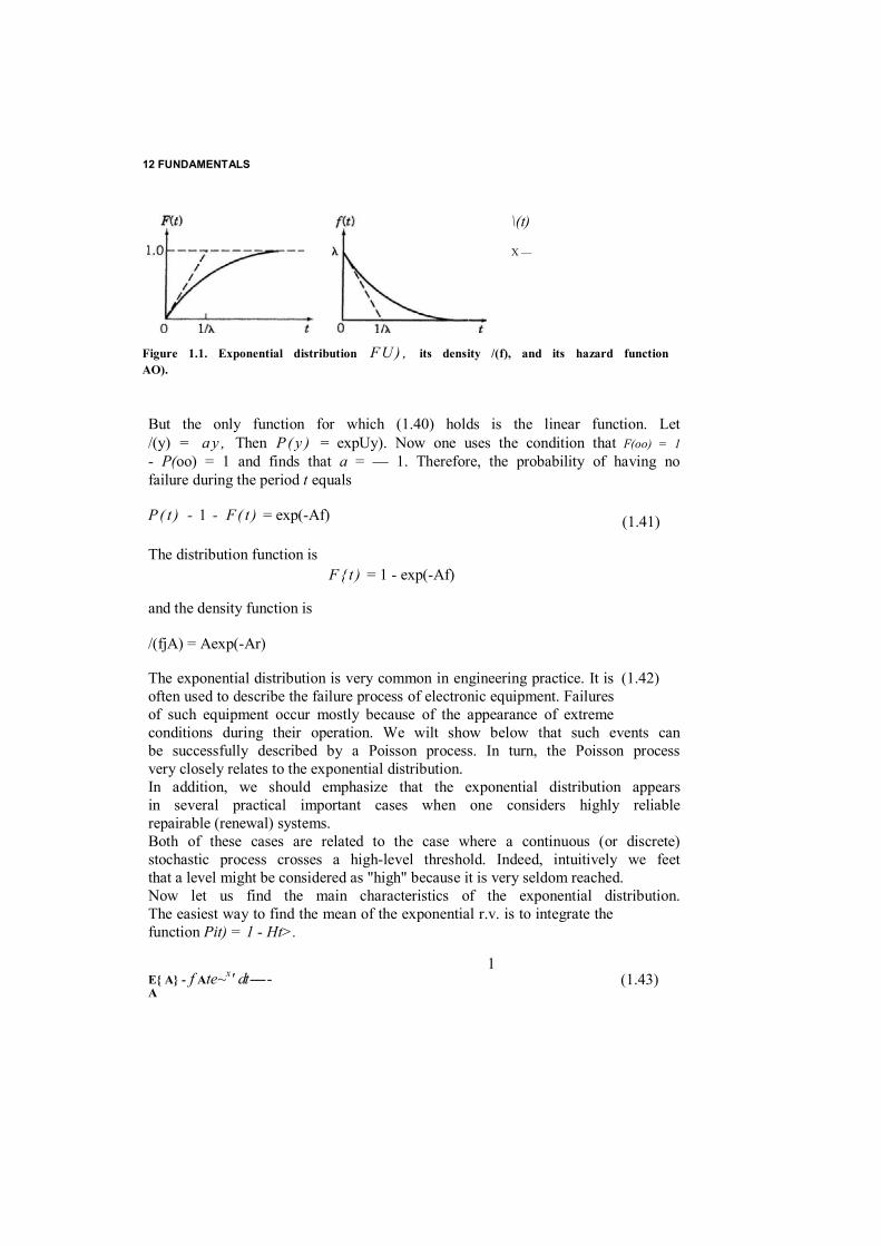
X —
Figure 1.1. Exponential distribution FU ) , its density /(f), and its hazard functionAO).
(1.43)
(1.41)
(1.42)

CONTINUOUS DISTRIBUTIONS RELATED TO RELIABILITY 13
The second initial moment of the distribution can also be found in a direct way
go 2 E{*2} = Ckt2e~x' dt = — (1.44) Jo A
and, consequently, from (1,43) and (1.44)
2 1 1 V**) - ? - y - p
that is, the standard deviation of an exponential distribution equals the mean
<7= Vv^W = ~
The m.g.f. for the density can also be found in a direct way (1.45)
J0 A - s
For future applications it is convenient to have the Laplace-Stieltjes transform (LST) of a density function. For the density of an exponential distribution, the LST equals
A <p(s) = [ \e~k'e~s' dt = ------------- (1.46) w Ja A + s x '
As we considered above, the LST of the function P i t ) = 1 - F i t ) = e A', taken at s = 0, equals the mean. In this case
<M 0 = / d t = (1.47)
and, consequently,
<Pp(s — 0) = T
One very important characteristic of continuous distributions is the inten- sity function which, in reliability theory, is called the failure rate. This function is determined as the conditional density at a moment t under the
14 FUNDAMENTALS
condition that the r.v. is not less than /. Thus, the intensity function is
l - F{ t ) - P i t )
For the exponential distribution the intensity function can be written as
/(0 no
that is, the failure rate for an exponential distribution is constant. This follows as well from the memoryless property. In reliability terms it means, in particular, that current or future reliability properties of an operating piecc of equipment do not change with time and, consequently, do not depend on the amount of operating time since the moment of switching the equipment on. Of course, this assumption seems a little restrictive, even for "exponential addicts." But this mathematical description is sometimes practically suffi- cient.
1.2.2 Erlang Distribution The Erlang distribution is the continuous analogue of a negative binomial distribution. It represents the sum of a fixed number of independent and exponentially distributed r.v.'s. The principal mathematical model for the description of queuing processes in a telephone system is a Markov one. Consider a multiphase stage, or example, a waiting line of messages. An observed message can stand in line behind several previous ones, say N. Then for this message the waiting time can be represented as a sum of the N serving times of the previous messages. By assumption, for a Markov-type model, each of these serving times has an exponential distribution, and so the resulting waiting time of the message under consideration has an Erlang distribution.
The sum of N independent exponential r.v.'s forms an Erlang distribution of the Nth order. It is then clear that the mean of an r.v. with an Erlang distribution of the jVth order is a sum of N means of exponential r.v.'s, that is,
A ( 0 - (1.48)= A

CONTINUOUS DISTRIBUTIONS RELATED TO RELIABILITY 15
B { X) = j (1.49)
16 FUNDAMENTALS
and so the variance equals N times the variance of a corresponding exponen- tial distribution
Var{X> (1.50)
Finally, the LST of the density of an Erlang distribution of the Nth order is
*(*) - (1.51)
The last expression allows us to write an expression for the density function of this distribution
(e.g., one can use a standard table of the Laplace-Stieltjes transforms). We will show the validity of (1.52) below when we consider a Poisson process.
Note that if the exponential r.v.'s which compose the Erlang r.v, are not identical, the resulting distribution is called a generalized Erlang distribution. Here we will not write the special expression for this case but one can find related results in Section 1.6.7 dedicated to the so-called death process.
1.2.3 Normal Distribution This distribution occupies a special place among all continuous distributions because many complex practical cases can be modeled by it. This d.f, is often termed a Gaussian distribution.
The central limit theorem of probability theory states that the sum of independent r.v.'s under some relatively nonrestrictive conditions has an asymptotically normal distribution. This fundamental result has an intriguing history which has developed over more than two centuries.
A simple example of a practical application of the central limit theorem in engineering occurs in the study of the supply of spare parts. Assume that some unit has a random time to failure with an unknown distribution. We know only the mean and variance of the distribution. (These values can be estimated, even with very restricted statistical data.) If we are planning to supply spare parts over a long period of time, as compared to the mean time to failure (MTTS) of the unit, we can assume that the total time until exhaustion of n spare units has an approximately normal distribution. This approximation is practically irreproachable if the number of planned spare parts, n, is not less than 30.

CONTINUOUS DISTRIBUTIONS RELATED TO RELIABILITY 17
In engineering practice the normal distribution is usually used for the description of the dispersion of different physical parameters. For example, the resistance or electrical capacity of a sample of units is often assumed to be normally distributed; the normal distribution characterizes the size of mechanical details; and so on. Incidentally, many mechanical structures exposed to wear are assumed to have a normal d.f. describing their time to failure. The normal distribution of the random time to failure OTP) also appears when the main parameter changes linearly in time and has a normal distribu- tion of its starting value. (The latter phenomenon was mentioned above.) In this case the time to the excedance of a specified tolerance limit will have normal distribution. We will explain this fact in mathematical terms below. The normal distribution has the density function
U x \ a , « ) - —JLe-U-ft**1 (1.53) (T\ ZT T
where a and a1 are the mean and the variance of the distribution, respec- tively. These two parameters completely characterize the normal distribution. The parameter u is called the standard deviation. Notice that cr is always nonnegative. From (1.53) one sees that it is a symmetrical unimodal function; it has a bell-shaped graph (see Figure 1.2). That a and a2 are, respectively, the mean and the variance of the normal distribution can be shown in a direct way with the use of (1.53). We leave this direct proof to Exercises 1.2 and 1,3. Here we will use the m.g,f.
00 1 <p„(s) = f —J=e-(x-ait/2a2esx dx = exp( a s + ± e r 2 s 2 ) (1.54)
.— oo <T\1tt
(The proof of this is left to Exercise 1.4.)
Fit) fit)
Figure 1.2. Normal distribution F(f), its density /((), and its hazard function A(()-
18 FUNDAMENTALS
From (1.54) one can easily find
and
VarfA*} = a2 (1.57)
[The proof of (1.56) is left to Exercise 1.5.] In applications one often uses the so-called standard normal d.f. In this case a = 0 and a = 1. It is clear that an arbitrary norma! r.v. X can be reduced to a standard one. Consider the new r.v. X' = X - a (obviously, the variances of X and X' are equal) and normalize this new r.v, by dividing by cr. In this way an arbitrary normal distribution can be reduced to the standard one (or vice versa) by means of a linear change of scale and changing the location of its mean to 0. The density of a normal d.f. is (see Figure 1.2)
<T\LTT
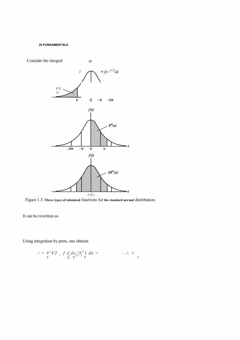
The function (1.58) has been tabulated in different forms and over a very wide range (see Fig. 1.3). Using the symmetry of the density function, one can compile a table of the function
e<*) = f f n ( x $ , \ ) d x J n J0
The correspondence between the functions F n ( x ) and F * ( x ) is
Often one can find a standard table of the so-called Laplace function: I — 2 F( x ) . This kind of table is used, for instance, in artillery calculations to find the probability of hitting a target. The distribution function of a normal distribution decreases very rapidly with increasing x. Most standard tables are, in fact, composed for Ul < 3 or 4, which is enough for most practical purposes. But sometimes one needs
E{*} =
EM «
(1.55)
(1.56)
■= a dz
d2<Pn(
z ) = a2 + cr2
clz z = 0

CONTINUOUS DISTRIBUTIONS RELATED TO RELIABILITY 19
values for larger x. In this case we suggest the following iterative computa- tional procedure.
20 FUNDAMENTALS
Consider the integral
/ = fe~x2'2dx
It can be rewritten as
Using integration by parts, one obtains
/ = V ' V 2 _ f J - f e - ' V 2 1 d x = - / , < t J , x 2 1 1 t t
m
F Xx )
-x 0 x Figure 1.3. Three types of tabuiated functions for the standard normal distribution.

CONTINUOUS DISTRIBUTIONS RELATED TO RELIABILITY 21
/. = \e-tn _ 3 dx = -L-'1'2 - /, < 1 f 3 J , x 4 r r
Thus at this stage of the iteration
I 1 7 - 7 3
More accurate approximations can be obtained in an analogous manner.
1.2.4 Truncated Normal Distribution A normal d.f. ranges from -00 to +<*>. But in reliability theory one usually focuses on the lifetime of some object, and so we need consider distributions defined over the domain [0, + <»). The new d.f. (see Fig. 1.4) is said to be "truncated (from the left)." The new density function, f(x\a, <r), can be related to the initial one, f{x\a, A), as follows:
In practical problems this truncation often has a negligible influence if a/cr is greater than 4 or 5.
The mean of a truncated distribution is always larger than the mean of its related normal distribution. The variance, on the other hand, is always smaller. We will not write these two expressions because of their complex form.
1.2.5 Weibull - Gnedenko Distribution One of then most widely used distributions is the Weibull-Gnedenko distri- bution. This two-parameter distribution is convenient for practical applica- tions because an appropriate choice of its parameters allows one to use it to describe various physical phenomena. One of the parameters, A, is called the scale parameter and another, (3, is called the shape parameter of the
Now we can evaluate I
and after integration by parts
I >
0

CONTINUOUS DISTRIBUTIONS RELATED TO RELIABILITY 23
distribution. A Wcibull-Gnedenko distribution has the form
F( t \ = h -e-(At)fi for t > 0 V ; \ 0 for / < 0
The density function is
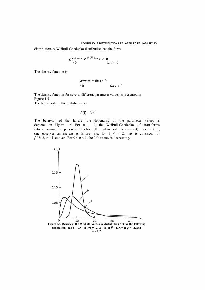
X'frP-ie-** for t > 0 \ 0 for t < 0
The density function for several different parameter values is presented in Figure 1.5. The failure rate of the distribution is
A(f) - A^"1
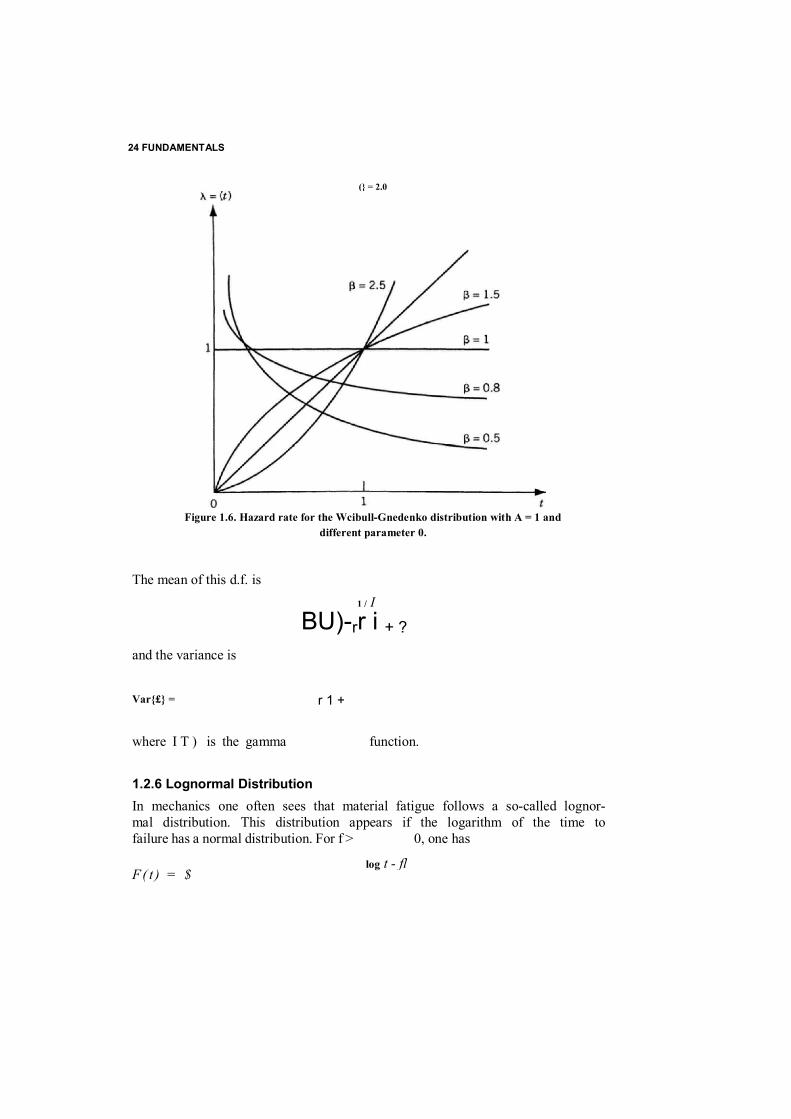
The behavior of the failure rate depending on the parameter values is depicted in Figure 1.6. For ft — I, the Weibull-Gnedenko d.f. transforms into a common exponential function (the failure rate is constant). For fi > 1, one observes an increasing failure rate: for 1 < < 2, this is concave; for [5 3: 2, this is convex. For 0 < 0 < 1, the failure rate is decreasing.
f ( t )
Figure t.5. Density of the Weibull-Gnedenko distribution /(r) for the following parameters: (a) 0 - 1, A - I; (fr) p - 2, A - 1; (c) P - 4, A = 1; p =* 2, and
A = 0,7.
24 FUNDAMENTALS
The mean of this d.f. is
1 / I
BU)-rr i + ? and the variance is
Var{£} =
where I T ) is the gamma function.
1.2.6 Lognormal Distribution In mechanics one often sees that material fatigue follows a so-called lognor- mal distribution. This distribution appears if the logarithm of the time to failure has a normal distribution. For f > 0, one has
F( t ) = $
(} = 2.0
Figure 1.6. Hazard rate for the Wcibull-Gnedenko distribution with A = 1 and different parameter 0.
r 1 +
log t - fl
CONTINUOUS DISTRIBUTIONS RELATED TO RELIABILITY 25
and the density is
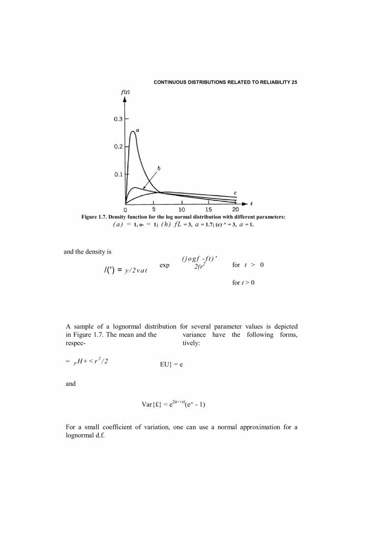
A sample of a lognormal distribution for several parameter values is depicted in Figure 1.7. The mean and the variance have the following forms, respec- tively:
= p H + < r 2 / 2
and
Var{£} = e2it+<rl(e^ - 1)
For a small coefficient of variation, one can use a normal approximation for a lognormal d.f.
Figure 1.7. Density function for the log normal distribution with different parameters: ( a ) = 1, o- = 1; ( h ) f L = 3, a = 1.7; (c) ^ = 3, a = 1.
( j o g f - f t ) ' 2(r2 for t > 0
for t > 0
exp /(') = y / 2 v a t
EU} = e
26 FUNDAMENTALS
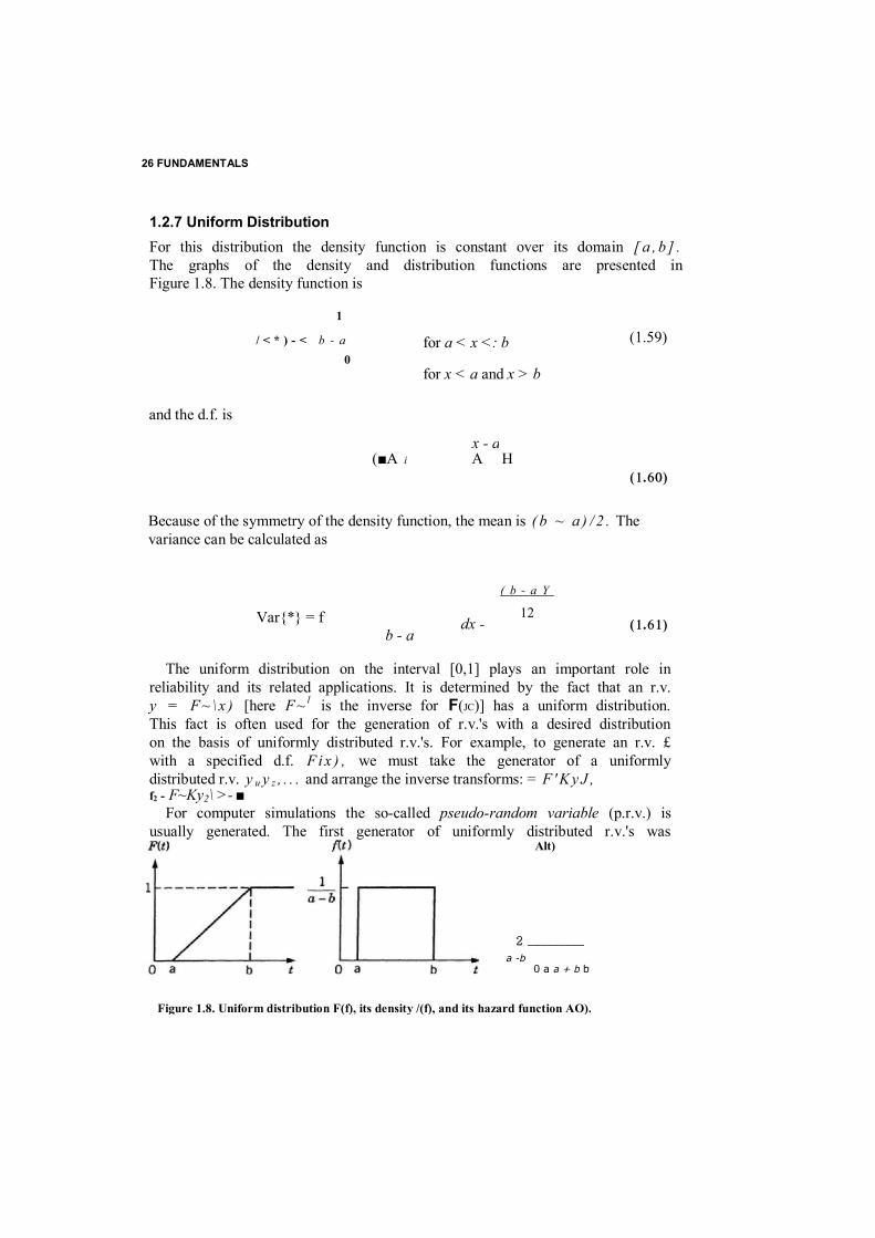
1.2.7 Uniform Distribution For this distribution the density function is constant over its domain [ a , b ] . The graphs of the density and distribution functions are presented in Figure 1.8. The density function is
1
for a < x <: b
for x < a and x > b
and the d.f. is
(■A i A H
(1.60)
Because of the symmetry of the density function, the mean is ( b ~ a ) / 2 . The variance can be calculated as
Var{*} = f
The uniform distribution on the interval [0,1] plays an important role in
reliability and its related applications. It is determined by the fact that an r.v. y = F~ \ x ) [here F~ l is the inverse for F(JC)] has a uniform distribution. This fact is often used for the generation of r.v.'s with a desired distribution on the basis of uniformly distributed r.v.'s. For example, to generate an r.v. £ with a specified d.f. F i x ) , we must take the generator of a uniformly distributed r.v. y u y z , . . . and arrange the inverse transforms: = F ' K y J , f2 - F~Ky2\ >- ■
For computer simulations the so-called pseudo-random variable (p.r.v.) is usually generated. The first generator of uniformly distributed r.v.'s was
/ < * ) - < b - a 0
(1.59)
x - a
( b - a Y
12 (1.61)dx -
b - a
a -b
Figure 1.8. Uniform distribution F(f), its density /(f), and its hazard function AO).
Alt)
2 _________
0 a a + b b
THE SUMMATION OF RANDOM VARIABLES 27
0 0
introduced by John von Neuman. The principle consists in the recurrent calculation of some function.
For example, one takes an exponential function with some two-digit power, chooses, say the 10th and 11th digits as the next power, and repeats the procedure from the beginning. Of course, such a procedure leads to the formation of a cycle: as soon as the same power appears, the continuation of the procedure will be a complete repetition of one of the previous links of p.r.v.'s. At any rate, it is clear that the cycle cannot be larger than 100 p.r.v.'s if the power of the exponent consists of two digits. Fortunately, modern p.r.v. generators have practically unrestricted cycle lengths.
At the same time, p.r.v.'s are very important for different numerical simulation experiments designed for comparison of different variants of a system design. Indeed, one can completely repeat a set of p.r.v.'s by starting the procedure from the same initial state. This allows one to put different system variants into an equivalent pseudo-random environment. This is important to avoid real random mistakes caused by putting one system in a more severe "statistical environment" than another.
1.3 SUMMATION OF RANDOM VARIABLES
The summation of random variables often comes up in engineering problems involving a probabilistic analysis. The observation of a series of time se- quences or the analysis of the number of failed units arriving at a repair shop are examples. At the same time, the number of terms in the sum is not always given—sometimes it is random. Asymptotic results are also of practical interest.
1.3.1 Sum of a Fixed Number of Random Variables General Case Consider a repairable system which is described by cycles as "a period of operation" and "a period of repair." Each cycle consists of two r.v.'s £ and TJ, a random time to failure (TTF) with distribution F ( t ) , and a random repair time with distribution G i t ) , respectively. If the distribution of the complete cycle is of interest, we would analyze the sum 6 = £ + 77. The distribution of this new r.v., denoted as D ( t ) = Pr{0 < t }, is the convolution of the initial d.f.'s:
= G * F( t ) = f ' G ( t — x ) d F{ x )
28 FUNDAMENTALS
If the Laplace-Stieltjes transforms (LSTs) of these d.f.'s
< P F ( s ) - f ' ° F( t ) e ~ s t d t Jo
and
<PCG(S) = f°°G(t)e~" dt Jo
are known, the LST of the d.f. D ( t ) is
{ p D ( S) =
If one considers a sum of n i.i.d. r.v.'s, the convolution F * " ( t ) is
Pr{ E Pr{ £ ftSf-Jc)dF(x)
Jo
where all JF* 's are determined recurrently. For a sum of i.i.d. r.v.'s each of which has LST equal to <p(s),
<PN (S ) - [?(*)] "
For the sum of n r.v.'s with arbitrary distributions, one can write
E{^} = E{ E £;} = E EU,} (1.62)
and, for independent r.v.'s.
J E (1-63) V lsjsn
Now we begin with several important and frequently encountered special cases.
Sum of Binomial Random Variables Consider two binomially distributed r.v.'s and v 2 obtained, respectively, by and n 2 Bernoulli trials with the same parameter q . From (1.21), the g.f. of the binomial distribution is
£(s) = ( p z + q)n> ( = 1,2 (1.64)
THE SUMMATION OF RANDOM VARIABLES 29
Thus,
$ ( z ) = <p,(z)<p2(z) = ( p z + q ) n \ p z + q ) " 2 = ( pz + q)"'+"2 (1.65)
In other words, the sum of two bionomially distributed r.v.'s with the same parameter p will produce another binomial distribution. This can be easily explained: arranging a joint sample from two separate samples of sizes n} and n 2 from the same population is equivalent to taking one sample of size n , + n 2 . Obviously, an analogous result holds for an arbitrary finite number of binomially distributed r.v.'s. Thus, we see that the sum of binomially dis- tributed r.v.'s with the same parameter p produces a new binomially dis- tributed r.v. with the same p and corresponding parameter
n = £ n i l Z j Z N
For different binomial distributions, the result is slightly more complicated (see Exercise 1.8).
Sum of Poisson Random Variables Consider the sum Xz of two inde- pendent Poisson r.v.'s Xx and X2 with corresponding parameters A,, i = 1,2. The m.g.f.'s for the two Poisson distributions are written as
V i ( z ) = e W- e "> i — 1,2 (1.66)
The m.g.f. for the distribution of the sum Xz can be written as
< p ( z ) = ^ ' - l ^ A ^ ' - l ) = e ( A 1 + A 3 X ^ - l ) (1.67)
that is, the resulting m.g.f. is the m.g.f. of a new Poisson d.f. with parameter Az = A, + A2. An analogous result can be obtained for an arbitrary finite number of Poisson r.v.'s. In other words, the sum of N Poisson r.v.'s is again a Poisson r.v. with parameter equal to the sum of the parameters:
A = £ A,- (1.68) 1
Sum of Normal Random Variables The sum of independent normally distributed r.v.'s has a normal distribution. Again consider a sum of two r.v.'s. Let Xj be a normal r.v. with parameters «, and ait i = 1,2, and let
30 FUNDAMENTALS
^ z ~ + X 2 - Then the m.g.f. for X can be expressed as
= Vi(2)p2(z) ™ exp(a,z + \a}z2) exp(a,z + \a\z2)
= exp[ + a 2 ) + ±z2(<rf + cr22)] (1.69)
Therefore, the sum of two normal r.v.'s produces an r.v, with a normal distribution. For n terms, the parameters of the resulting norma! distribution are
(1.70) az - £ Of
J s i s N
and
(1.71) V ts/sAf
1.3.2 Central Limit Theorem Many statisticians have worked on the problem of determining the limit distribution of a sum of r.v.'s. This problem has practical significance be- cause, when a sum includes a large number of r.v.'s, the direct calculation of some characteristic of the sum becomes very complicated. The problem itself has aroused theoretical interest even outside of applications. Above we showed that a sum of different normally distributed independent r.v.'s has a normal distribution, independent of the number of terms in the sum. The new resulting normal distribution has a mean equal to the sum of the means of the initial distributions and a variance equal to the sum of the variances. It is obvious that this property is preserved with the growth of n. But what will be the limiting distribution of a sum of r.v.'s whose distribu- tions arc not normal? It turns out that, with increasing n, such a sum has a tendency to converge to a normally distributed r.v. In simple engineering terms it appears that if we consider a sum of a large number n of independent r.v.'s then this sum has approximately a normal distribution. If we consider the sum of independent arbitrary distributed r.v.'s £ with mean a = E{£) and variance v = Var{£), then the normal distribution of the sum will have mean A = an and variance V — un. (Of course, some special restrictions on the independence and properties of distributions must be fulfilled.) Historically, limit theorems developed over several centuries. Different versions of them pertain to different cases. One of the first attempts in this direction is contained in the following theorem.
<rN =
THE SUMMATION OF RANDOM VARIABLES 31
DeMoivre Local Theorem Consider a sequence n of Bernoulli trials with a probability of success p. The probability of m successes P„(m) satisfies the relationship
_____ g —K / * y/2tt
uniformly for all m such that
m — np
yfnpq
belongs to some finite interval. This theorem, in turn, is the basis of the following theorem.
Integral DeMoivre - Laplace Theorem If v is the random number of successes among n Bernoulli trials, then for finite a and b the following relationship holds:
The next step in generalizing the conditions under which the sum of a sequence of arbitrary r.v.'s converges to a normal distribution is formulated in the following theorem.
Liapounov Central Limit Theorem Suppose that the r.v.'s X, are inde- pendent with known means ai and variances or,2, and for ail of them, EffA^ — at< <*>. Also, suppose that
E lim -------------- = 0
V v Uisn '
Then, for the normalized and centered (with zero mean) r.v.,
i32 FUNDAMENTALS
for any fixed number x,
n
Thus, this theorem allows for different r.v.'s in the sequence and the only restrictions are in the existence of moments of an order higher than 2. As a matter of fact, this statement is true even under weaker conditions (the restriction of a variance is enough) but all r.v.'s in the sum must be i.i.d. For the sample mean, the related result is formulated in the following theorem.
Lindeberg - Levy Central Limit Theorem If the r.v.'s Xt are chosen at random from a population which has a given distribution with mean a and finite variance a 2 , then for any fixed number y ,
t i f c ( X „ - a ) \ 1 r y Iim Pr ------ ^ -------- < y = f e ~ z d z
y <j ) v2tt j - x
where X„ is the sample mean. Because
this theorem may be interpreted in the following way: the sum of i.i.d. r.v.'s approximately has a normal distribution with mean equal to na and variance equal to n a 2 . A detailed historical review on the development of probability theory and statistics can be found in Gnedenko (1988).
1.3.3 Poisson Theorem
Considering the locaf DeMoivre theorem, we notice that this result works well for binomial distributions with p close to 1/2. But the normal approxi- mation does not work well for small probabilities or on the "tails" of a binomial distribution. An asymptotic result for small p (for the "tails" of the binomial distribution) is formulated in the following theorem.
iim Pr{Y„ < JC} =
THE SUMMATION OF RANDOM VARIABLES 33
Poisson Theorem If pn -» 0 with n -» then
where an — np,
34 FUNDAMENTALS
This means that for small p, instead of calculating the products of astronomically large binomial coefficients with extremely small p", we can use a simple approximation. A standard table of the Poisson distribution can be used.
1.3.4 Random Number of Terms in the Sum Only a very general result can be given for the d.f. of the sum of r.v.'s, or for its LST when a random number of terms is distributed arbitrarily. Further, let us assume that v is geometrically distributed. Then the distribution of the sum of arbitrarily distributed r.v.'s is
P r f o * ' } - E p W E L z t )
Consider a continuous d.f. The LST can be written as
< Pz { s ) = £ p k q [ < p ( s ) ] k t zkzN
In general, both of the latter expressions are practically useful only for numerical calculation. To find the mean of we may use the Wald equivalence:
E{ E f*)=E{»}EU} (1-72)
Below we consider two cases where the sum of finite r.v.'s will lead to simple results.
Geometrically Distributed Random Variables We can investigate this case without using a mathematical technique. Consider an initial sequence of Bernoulli trials. The probability of success equals p and the probability of failure equals q = 1 - p. Now construct the new process consisting of only failures of the initial process and corresponding spaces between them. Consider a new procedure: each failure in the initial Bernoulli process creates a possibility for the appearance of a failure in the final process. (Failure cannot appear in the space between failures of the initial process.) A special moment concerning the "possibility" of a new process failure is considered. Let a failure of the initial process develop into a failure of the new (final) process with probability Q. Thus, if we consider the initial process, failure of the final process occurs there with probability Q* = qQ. We have obtained this result using only verbal arguments. Of course, it can be derived in strict mathematical terms.
THE SUMMATION OF RANDOM VARIABLES 35
Exponentially Distributed Random Variables Consider the sum of a random number of exponentially distributed identical and independent r.v.'s, with parameter A. Assume that the number of terms in the sum has a geometric d.f. with parameter p . We will express the LST of the resulting density function through the LST of the density function of the initial d.f. From the formula for the complete mathematical expectation, we have
A A2 A3 = q .. ........ + pq -------------- + ---------- + • ■ • ' y A ™ ( k + s f ( A +s)3
_ y ( P A ) k _ < ? A 1 = <?A . J 7 3 A + * (A + s ) k s + £?A A + s
Thus, we have an expression which represents the LST for an exponential distribution with parameter A = Aq. We illustrate the usefulness of this result by means of a simple example. Imagine a socket with unit installed. Such a unit works for a random time, distributed exponentially, until a failure occurs. After a failure, the unit is replaced by a new one. The installation of each new unit may lead to a socket failure with probability q. This process continues until the first failure of the socket. This process can be described as the sum of a random number of exponentially distributed random variables where the random number has a geometrical distribution. Of course, in general, the final distribution of the sum strongly depends on the distribution of the number of terms in the sum. The distribution of the number of terms in the sum is the definitive factor for the final distribution.
1.3.5 Asymptotic Distribution of the Sum of a Random Number of Random Variables In practice, we often encounter situations where, on the average, the random number of terms in the sum is very large. Usually, the number of terms is assumed to be geometric. If so, the following limit theorem is true.
Theorem 1.1 Let {£} be a sequence of i.i.d. r.v.'s whose d.f. is F i t ) with mean a > 0. Let v be the number of discrete r.v.'s of a sequence with a geometric distribution with parameter p : Pr{f = k ) = ( i p k ~ ] where q — 1 — p. Then, if p -* 1, the d.f. of the normalized sum
^E ~ Q £ U lstip
converges to the exponential d.f. 1 — e~1''.
36 FUNDAMENTALS
Proof. Consider the normalized r.v.
E & 6z £
i<.k<.v
By the Wald equivalency,
e{ L | = E{f} E{£} Without loss of generality, we can take E{£} = 1. Because v has a geometric distribution, E{P) = l / q . Hence,
1 E i k 1 s k s v
The LST of is
= E{<r^} = E j ex p / ~qs £
E p k ~ ] q e x p E f t )
Note that
expj ~qs E ft) = [?(*?)]'
Then
= E p k ~ l e[ < p ( w) ] k 1 sfc <0t>
- ) E [ P 9 { s q ) \ k = o 1 ~ P< p ( W )
Now with some simple transformations
. . q < p ( s q ) q<p{sq) = ------------------- —■——— -- -------------------------------------------------------------------------------------
1 - p < p ( s q ) 1 - < p ( s q ) + q < p ( s q )
< p ( s q ) 1 - <p(sq) s . . — + < p { s q )
s q

RELATIONSHIPS AMONG DISTRIBUTIONS 37
Notice that <pCj)|t_n = 1. Hence,
lim i p ( s q ) = 1
and, consequently,
1 - i p ( s q ) <p(0) - < p ( s q )
[jm ------- —-— = [im -------- — q — o s q t ) — o s q
Taking into account that E{£} = 1, we have finally
that is, has an exponential distribution with parameter A = L
1.4 RELATIONSHIPS AMONG DISTRIBUTIONS
Various distributions have common roots, or are closely related. As we discussed previously, the normal and exponential distributions serve as asymptotic distributions in many practical situations. Below we establish some connections among different distributions that are useful in reliability analysis.
1.4.1 Some Relationships Between Binomial and Normal Distributions The De Moivre-Laplace theorem shows that, for large n when min(«< 7, n p ) » 1, the binomial distribution can be approximated by the normal distribu- tion.
Example 1.1 A sample consists of n = 1000 items. The probability that the item satisfies some specified requirement equals Pr{success} - p - 0.9. Find Pr{880 < number of successes}.
Solution. For the normal d.f. which approximates this binomial distribution, we determine that a = np = 900 and a2 = npq = 90, that is, a ~ 9.49. Thus,
/ 880 - 900 \ Pr{880 <*} = !-4>[ 949 )
880 - 900
-<p'(0) = -H|f}

38 FUNDAMENTALS
= 1 - <t>( -2.11) = 1 - 0.0175 = 0.9825

RELATIONSHIPS AMONG DISTRIBUTIONS 39
Example 1.2 Under the conditions of the previous example, find the num- ber of good items which the producer can guarantee with probability 0.99 among a sample of size n = 1000.
Solution. Using a standard table of the normal distribution, from the equa- tion
x - 900 + 0.5 \ ( x - 900.5 Pr(m >;*> " ^900 " = 0 01
we find
x - 900.5 » -2.33
9.49
or x = 978.6. Thus, the producer can guarantee not less than 978 satisfactory items with the specified level of 99%. We must remember that such an approximation is accurate for the area which is more or less close to the mean of the binomial distribution. This becomes clear if one notices that the domain of a normal distribution is (—oo, <»), while the domain of a binomial distribution is restricted to [0, n). In addition, there is an essential difference between discrete and continu- ous distributions. Thus, we must use the so-called "correction of continuity":
a ifnpq j \ ifnpq
1.4.2 Some Relationships Between Poisson and Binomial Distributions By the Poisson theorem, a Poisson distribution is a good approximation for a bionomial distribution when p (or q ) is very small.
Example 1.3 A sample consists of n — 100 items. The probability that an item is defective is equal to p = 0.005. Find the probability that there is exactly one defective item in the sample.
Solution. Compute a = 100 • (0.005) = 0.5. From a standard table of the Poisson distribution, we find p(l;0.5) — 0.3033. The computation with the use of a binomial distribution gives
p h ( l ' , 0.005, 100) = ( j0.005 • 0.9959" ® 0.5e"°-5
» (0.5) • (0.6065) m 0.3033
40 FUNDAMENTALS
1.4.3 Some Relationships Between Erlang and Normal Distributions The normal approximation can be used for the Erlang distribution when k is large, for instance, when k is more than 20. This statement follows from the "Lindeberg form" of the central limit theorem. Let Y be an r.v. with an Erlang distribution of the k th order. In other words, Y — X , + X 2 + ■ • • + X k where all AT/s are i.i.d. r.v.'s with an expo- nential distribution and parameter A. Then, if k » 1, Y approximately has a normal distribution with mean a = k / k and standard deviation c r = if a .
Example 1.4 Consider a socket with 25 units which replace each other after a failure. Each unit's TTF has an exponential distribution with parameter A = 0.01 [1/hour], Find the probability of a failure-free operation of the socket during 2600 hours. (Replacements do not interrupt the system opera- tion.)
Solution. The random time to failure of the socket approximately has a normal d.f. with parameters a = 25 ■ 100 = 2500 hours and <r = ^(2500) = 50 hours. The probability of interest is
1.4.4 Some Relationships Between Erlang and Poisson Distributions Consider the two following events:
(a) We observe a Poisson process with parameter A. The probability that during the interval [0, r] we observe k events of this process is
( A O
(b) We observe an r.v, £k with an Erlang distribution of order k with parameter A. Consider the event that £ is smaller than f and, at the same time, + 1 is larger than t. The probability of the latter event equals
[A(f -x)]* ' e~Mt-*>e-x* dx
= - P p ( k - , k t )
RELATIONSHIPS AMONG DISTRIBUTIONS 41
Thus, events (a) and (b) are equivalent. It is important to remark that both the Erlang r.v. and the Poisson process are formed with i.i.d. r.v.'s with exponential d.f.'s.
Notice that the unconditional event £k > t is equivalent to the set of the following events in the Poisson process: {no events arc observed) or {one event is observed) or {two events are observed) or... or {k - 1 events are observed). This leads to the following condition:
(Af) Z = / > , ( * - ! ; A * ) n t ■
or, for the probability of the event fk < t, that is, for the d.f, of the Erlang r.v. of the fcth order, we have
Therefore, in some sense, the Poisson d.f. is a cumulative function for an r.v. with an Erlang distribution.
1.4.5 Some Relationships Between Poisson and Normal Distributions Note that a high-ordered Erlang r.v. can be approximated by a normal r.v. and, at the same time, it has a Poisson distribution as its cumulative distribution. This fact can be used as a heuristic justification for the possibil- ity of approximating a Poisson distribution with the help of a normal distribution. The strict proof of this statement can be obtained with the help of a Gram-Charlie set (see below).
Here we take without proof that a Poisson distribution can be approxi- mated by a normal distribution. For a Poisson d.f. with a large mean a, the approximation can be written as
Notice that this approximation is accurate in an area close to the mean and may be very bad for the "tails" of the Poisson distribution. This is explained by the fact that these two distributions have different domains: the normal distribution is defined on (-00,00), while the Poisson d.f. has no meanings for m < 0.
Example 1.5 Assume that the number of failures of some particular unit of equipment has a Poisson distribution. The expected number of failures
k - 1
P r { & > * } = = Z
0

42 FUNDAMENTALS
during a specified period of time equals 90. One has decided to supply the

RELATIONSHIPS AMONG DISTRIBUTIONS 43
equipment with 100 spare units of this type. With what probability will there be no deficit of spare units?
Solution.
I 100 - 90
PrH^lOO}
From a standard table of the normal distribution, we find that this probability equals 0.853.
Example 1.6 Under the conditions of the previous example, find how many spare units should be supplied so that the probability exceeds 0.995.
Solution.
I x ~ 90 + 0.5 \ Pr [ m > x } ~ 4>| -- ----- J - 0-995
From a standard table of the normal distribution, we find that
a: - 90.5 = 2.576
\/90
or jc = 114.9. This means that one should have 115 spare units.
1.4.6 Some Relationships Between Geometric and Exponential Distributions It is clear that an exponential distribution is an approximation to a geometric distribution with q — A Ac
lim — [(1 - A A t ) ' / A ' \ A f l = A Um (1 - A &t ) ' / A ' = \ e ~ A ' m-O A r L 1 &t->o
where At 0.
1.4.7 Some Relationships Between Negative Binomial and Binomial Distributions The relationship between these distributions is similar to the relationship between the Erlang and Poisson distributions. Consider a sequence of Bernoulli trials that forms a negative binomially distributed r.v. v k consisting of the sum of k geometrically distributed r.v.'s. Let us pay attention to the
= <t>( 1.05)
44 FUNDAMENTALS
first n trials where n > k . The event { v k > n} means that, in the first n trials, there are 0, or 1, or 2,... f or k - 1 failures, that is,
Pr K>«} = £ ("W"' O &j &k ~ 1 V J I
1.4.8 Some Relationships Between Negative Binomial and Erlang Distributions We noticed that the geometric distribution is related to the exponential distribution. In the same sense, the convolution of geometric distributions is related to the convolution of exponential distributions. No other comments are needed: the negative bionomial and Erlang distributions are these convo- lutions.
1.4.9 Approximation with the Gram-Charlie Distribution Because of the wide applications of the normal distribution, many attempts were made to use various compositions of this distribution to express other distributions. Below is one of them. Let /(/) be the density function of a distribution other than the normal distribution. The mean a and the variance cr1 of this distribution are known. Introduce a new variable
x - a t - ------------ (1.74)
<T
The density function /(t) can be represented with the help of the Gram-Charlie series
/ ( / ) ~A0<p{t) +A1<p'(t) + A 2 < p "( t ) + • • •
where <p(r), <p'(t), <p"(0,. . . are the density of the normal distribution and its subsequent derivatives. The standard normal density is expressed as
Introduce the Chebyshev-Hermit polynomials:
a>inHt) Hn(t) = (-1) —777- (1.75)
f(0
RELATIONSHIPS AMONG DISTRIBUTIONS 45
where c p u ' K t ) is the nth derivative of the normal density. By direct calcula- tions we find
H 0 ( 0
= 1
J f , ( 0 - t
H 2 ( t ) = t 2 - 1 (1.76)
H 3 ( t ) = r3 - 3 t
H 4 ( t ) = /4 - 6r2 + 3
Usually, for practical problems, we do not need more than four terms of the Gram-Charlie set. From (1.75) it follows that
These functions go to 0 for ail n when t - * ±», The functions ( p i t ) , H 2 , and H a are even, and the functions H, and are odd, so from (1.77) it follows that
< P ' ( ~ 0 = < P ( 0
< p " ( - 0= < P ( 0
<P{3)(-0 = -?(3)(r)
( p w ( - t ) = < p < 4 > ( t )
The Chebyshev-Hermit polynomials are orthogonal, that is,
This fact can be proven by direct calculation. Now substitute the Chebyshev-Hermit polynomials into (1.75)
f ( t ) - A 0 H 0 ( t ) v ( t ) - A M O v C O + A 2 H 2 ( t ) < p ( t ) ~ ■ ■ ■ (1.78)
To find A n , multiply both sides of (1.78) by H n ( t ) and integrate from — GO to oo. Because of the above-mentioned orthogonality property of the Chebyshev-Hermit polynomials, we have
( - 1 ) " A n = - - - - f f ( t ) H „( t ) d t (1.79)
n : J — oo
RELATIONSHIPS AMONG DISTRIBUTIONS 46
After substituting (1.76) into (1.79), we obtain
A 0 = \
A, = -m?
A 2 = - £ (1.80)
A t ~ _ i [ m o _ 3 m ? ]
= + 3]
where is the central moment on the /ith order of the r.v. t. Thus, m" = 0, m\ = 1, and, consequently, all initial moments are equal to centered moments. Then from (1.80)
A, - 0 A2 = 0
A 4 = ± [ m A ( t ) - 3] = s M O
where k3 and k4 are known as the coefficient of asymmetry and the coefficient of excess, respectively,
m i i x )
m 4 ( x )
k3 defines the deviation of the density function under consideration from a symmetrical function, and k4 defines the sharpness of the mode of the density function. All symmetric densities have k3 = 0, and a normal density has k4 = 0. Finally, we obtain
or, after integration from - QO to t,
F( t ) ~ < P( t ) - ik3<p<2>(t) + ±4k4<p«\t)
Notice that t is the linear function of x . And so, f i x ) and F ( x ) can be
STOCHASTIC PROCESSES 47
expressed as
f ( x ) - - cr
and
Example 1.7 With the help of the Gram-Charlie series, the Poisson distri- bution can be approximately expressed as
Pr{1 < c) m <t>(f) - + -24%<3>(/) (1.81)
where
x — a — 0.5 r =
and a is the parameter of the Poisson distribution. It is clear that for a 1 one can disregard the last two terms of the right side of (1.81), and, consequently, the Poisson distribution can be approxi- mated by the normal distribution for targe a .
REMARK. The Gram-Charlie distribution can be successfully applied to the evaluation of d.f.'s. This takes place, for instance, in analyses of the distribution of a parameter of a piece of electronic equipment when the distributions of its components are known.
1.5 STOCHASTIC PROCESSES
Stochastic processes are used for the description of a system's operation over time. There are two main types of stochastic processes: discrete and continu- ous. Among discrete processes, point processes in reliability theory are widely used to describe the appearance of events in time (e.g., failures, terminations of repair, demand arrivals, etc.). A well-known type of point process is the so-called renewal process. This process is described as a sequence of events, the intervals between which are
1 Stationarity • Memorylessness (Markov property) • Ordinarity

48 FUNDAMENTALS
i.i.d. r.v.'s. In reliability theory this kind of mathematical model is used to describe the flow of failures in time. A generalization of this type of process is the so-called alternating renewal process which consists of two types of i.i.d. r.v.'s alternating with each other in turn. This type of process is convenient for the description of renewal

STOCHASTIC PROCESSES 49
systems. For such systems, periods of successful operation alternate with periods of idle time.
The more complex process is a process describing a system transition from state to state. The simplest kind of such a process is a Markov process. If the times that the process may change states are assumed to be discrete, the process is called the Markov chain.
We start with simplest cases and move in the direction of more complex mathematical models.
1.5.1 Poisson Process In the theory of stochastic processes, the Poisson process plays a special role, comparable to the role of the normal distribution in probability theory. Many real physical situations can be successfully described with the help of a Poisson process. A classical example of an application of the Poisson process is the decay of uranium: radioactive particles from a nuclear material strike a certain target in accordance with a Poisson process of some fixed intensity.
In practice, the Poisson process is frequently used to describe the flow of failures of electronic equipment. In inventory control, the flow of random requests for replacement of failed units is also often assumed to be described by a Poisson process, especially if the system which generates these requests is large.
Sometimes the Poisson process is called "a process of rare events." Of course, the meaning of the word "rare" should be carefully defined in each particular case. Usually, we speak about rare events if they appear with a frequency which is lower than the frequencies of other accompanying pro- cesses. The Poisson process appears as the interaction of a large number of these processes and, consequently, has a frequency lower than the other processes.
In reliability, such "rare" events appear, for instance, when one considers a highly reliable renewal redundant system or a multicomponcnt renewal series system. This process also successfully describes the fluctuation over a high- level threshold.
This process is so named because the number of events in any fixed interval of length t has a Poisson distribution:
(A t ) k Pr{£ events during f} = p k ( t ) = - - - - - - - e A '
Ac! where A is called the parameter of the Poisson process.
First of all, note that the Poisson process possesses the three following properties that are often referred to as characterization properties:
50 FUNDAMENTALS
The first property means that the d.f. of the number of observed events in a time interval depends only on the length of the interval and not on its position on the time axis. The second property means that the d.f. of the number of observed events does not depend on the previous history of the process. The third property means that the probability of an appearance of more than one event in an infinitesimally small interval h goes to 0:
1 — Iim Pr{k events appear during h , k > 1} -» 0 h a - O
or, in another notation,
Pr{fc events appear during h , k > 1 } = o ( h ) (1.82)
In practical problems, these properties are often assumed. These proper- ties, which seem to be—at a first glance—purely qualitative, allow us to obtain strict mathematical results. First, for a better understanding, we present a semiintuitive proof of the fact that these properties generate a Poisson process. Consider a Bernoulli process with probability of success p and a sufficiently large number of trials n. The Bernoulli process satisfies the first two properties (and trivially satisfies the third one because of its discrete nature). As we considered in Section 1.1, the number of successes in a series of n Bernoulli trials has a binomial distribution. As we have shown in Section 1.1, for large n the binomial distribution can be successfully approximated by a Poisson distribu- tion. We now return to the exact mathematical terms. First, add one extra property to the above three properties, namely, assume that the probability that there is exactly one event in a time interval h:
Pj ( h ) = A h + o { h ) (1.83)
where A is some constant and o ( h ) was introduced in (1.82). As a matter of fact, (1.83) follows from the three properties characterizing a Poisson pro- cess. Consider the probability of the appearance of k events in a time interval t + h. The formula for the probability can be easily written as
P k ( t + h ) = z WWM 0-84) 0
Let
= E PjiOfW*> (1.85)

STOCHASTIC PROCESSES 51
0 z j < , k - 2
STOCHASTIC PROCESSES 52
R k S I P k - j ( h ) < L P , ( h ) (1.86) Q £ j £ k - 2 2 zi&k.
because all P s ( t ) < 1. We only reinforce the inequality (1.86) by changing the limits of summation
R k < L W)
= Pr{two or more events appear during interval h} (1.87)
At the same time, by assumption, this probability equals o ( t ) . As a result, we have the equality
W + h ) = P k ( t ) P Q ( h ) + P k . i ( t ) P 1 ( h ) +o(0 (1.88)
In this equality, we can substitute P t { h ) = \ h + o ( h ) . Also, P 0 ( h ) + P t (h) + o ( h ) = 1, that is, P Q ( h ) = 1 - Ah + o ( h ) . Now (1.88) can be rewritten as
P k ( t + h ) = P k ( 0 0 - Ah ) + P k - t ( t )AA + o ( t ) (1.89)
and from (1.89) we obtain
and, after h 0,
d P k { t ) = - \ P k ( t ) + \ P k ^ ( t ) (1.90)
d t
Thus, a system of equalities for P k ( t ) , k = 0, I,..., has been obtained. We need to add one more equation to determine P0(f). Using the memoryless property, we can write
pQ(t + h) = p 0 ( t ) p 0 ( h ) = p0(t)[ 1 - \ h + o ( h) 3
or, finally,
dPQ(t) = -AP0(0 (1-91)
d t
To solve the system, we must determine the initial condition. Of course, at t = 0, the probability of no events equals 1; that is, the initial condition is />,,( 0) = 1.
Obviously,

BIRTH AND DEATH PROCESS 53
The system of differential equations (1.90) and (1.91) with the above initial condition can be solved by several different methods. We solve this system of equations with the use of the LST. Let <p0(s) be the LST of the function PoO):
< p 0 ( j ) = f p 0 ( t ) e - "d t (1.92) J o
Applying (1.92) to (1.91) and keeping in mind the properties of the LST, one obtains
-/>o(0) + s < p 0 ( s ) = - \ < p 0 ( s ) (1.93)
which has the solution
< Po ( * ) = T — ( ! - 9 4> A + s
As it follows from a table of Laplace-Stieltjes transforms, the function P 0 ( t ) corresponding to (1.94) is exponential with parameter A:
P 0 ( t ) = e ~ » (1.95)
For arbitrary k > 0, from (1.90) the system of recurrent equations follows:
s < p k ( s ) = -A < p k ( s ) + A <?*_,(*) (1.96) or
Finally, using (1.94) systematically, we have
Ms) - + l (1.98) (A + 5 )
From a table of LSTs, the latter transformation corresponds to a Poisson distribution
( A/ ) * 4 P k ( t ) = (1.99)
For the Poisson distribution the mean number of events in a fixed interval of time is proportional to its length. The parameter A is the mean number of events in a time unit, or, equivalently, it equals the inverse of the mean time

54 FUNDAMENTALS
between events. Also, as known (see the Appendix), a convolution of Poisson distributions produces a Poisson distribution. Thus, for several disjoined intervals of lengths t x , t 2 , . . . , t m , the distribution of the total number of events is Poisson with parameter A(/, + t 2 + • * • + t m ) . In other words, the Poisson process is a point stochastic process with exponentially distributed intervals between neighboring events.
1.5.2 Introduction to Recurrent Point Processes We often encounter situations where some events occur sequentially in such a way that the times between occurrence (interarrival times) can be success- fully described by a sequence of independent r.v's. For instance, consider a socket with an installed unit which is instantly replaced upon failure by a new unit; the times between replacement moments form such sequence. In general, the length of each interval might depend on the number of the event because of a changing environment, a wearing out of the socket, and so on. Here we ignore such phenomena. A process of this type is called a point process with restricted memory.
A point process with restricted memory is a sequence of r.v.'s. It is called a renewal (recurrent) point process if all interarrival intervals are i.i.d. r.v.'s with identical d.f.'s F k ( t ) = F( t ) , k s 2, with only the first interval having its own distribution F x ( t ) .
The Poisson process represents a particular case of such a process in that the intervals between arrivals are independent and exponentially distributed.
We assume that a flow of failures is represented by a recurrent point process. This assumption is acceptable in many practical situations. At the same time, it allows us to obtain simple and understandable results.
For a renewal point process, there are two main characteristics: (1) the process intensity defined to be the mean number of process events arriving in a time unit and (2) the process parameter defined to be the limit probability of the arrival of at least one event.
Let N(r) be the number of events arriving during an interval of length t . Then, for the stationary process,
A* = lim -E{N(M + T)} = lim - £ j p X t , t + T) T r o<;y<°=
The parameter of the process is defined as
A = lim lim — £ P j ( t ) T 0 £ j < s c
For an arbitrary stationary point process with a single arrival at a time and without so-called "points of condensation" (infinitesimally small intervals in

BIRTH AND DEATH PROCESS 55
which an infinite number of discrete events might appear), we have
A* < A For a stationary and memoryless point process, the parameter coincides with the intensity. We can given an explanation of the parameter of a point process based on a more physical consideration:
A*(/) A = Pr{at least one failure occurs in [f, / + A]}
Let f * ( t ) stand for a convolution of the /cth order of the function /(f):
r \ t ) - f r ° ! - i \ x ) f ( t - x ) d x
it is clear that at least one failure might occur if
- The first failure occurs with probability /(/)A. • The second failure occurs with probability f * 2 ( t ) A,..., • The Arth failure occurs with probability f * k ( t ) A and so on.
Thus, the probability that a failure will occur for any of these reasons is
Pr{at least one failure occurs in the interval [/,/-»- A]} A*(/) A =
where we use the conditional notation /*°(f) =/(0. Hence,
A *( f ) - [ z r k ( t ) . t s o
The function A*(f) allows us to express the so-called characterization point process function which we denote by A*(f):
A*(M + r*) = f' + t * X * ( t ) d t J t
Using this function, we can write
Pr{no failures in [ f, t + t * ]} = exp
= _-A*('.< + <*> = _-[A*(/-w*)-A*(0] =
(1.100)
56 FUNDAMENTALS
The function A i t ) is defined to be the "instant" conditional density of the failure distribution F i t ) . We emphasize that the functions AO) and A* i t ) are quite different.
Now consider the main characteristics of a renewal process. One of the characteristics of a renewal process is the mean number of events occurring up to a moment t . Denote the random number of events by N i t ) and the mean number by H i t ) = E{ N i t ) ) . H i t ) is called the renewal function. The derivative h ' i t ) = H i t ) is called the renewal density. Consider a renewal process composed of i.i.d. r.v.'s with distribution F i t ) . We can write
Pr{N(r) £ A:} = £ ? r { N i T ) =;} = Pr{ £ < A = F**(r) k£j<<"> Ms/st '
where F* k i t ) is the &th-order convolution of F i t ) :
F* k i t ) = f' F* i k - l \ t - x ) d Fi x ) J o
JF* 1 - F i t )
The expression can be easily written as
Pr{any event occurs in interval [ t , t + dt\\ = E Pr{thc fcth event occurs in interval [r, t + d t ] )
= h i t ) d t = f i t ) d t + £ f * k i t ) d t (1.101) 2sk <oo
Integrating (1.101) allows us to write an expression for H i t ) :
H { t ) = F i t ) + £ F* k ( t ) (1.102) 2<.k <oo
Of course, H i t ) can be found in a standard way as the mean number of events during time f. The probability that exactly k events happen up to moment t is expressed as
Pr{N(0 = k ) = Pr{N(r) ;> Jt} - Pr{JV(r) £ k - 1}
= F* \ t ) - F*<* + 1 ) ( 0
BIRTH AND DEATH PROCESS 57
Thus, the distribution of N ( t ) is defined. H ( t ) can be found by
H ( t ) = E { N ( t ) } = E *P r { N ( r ) = fc } 1 f c < ° °
= E *[f**(0
= F(r) + E k F* k ( t ) - E ( k - l ) F* k ( t ) 2sk<<x> 2
- E F*k(0 1 <«>
For h i t ) we can write
Pr{any event occurs in interval [t,t + At]}
= Pr{the first event occurs in interval [ t , t + A]}
+ Pr{thc last event happens in interval [ t , t + A t ] (1.103)
and the following random time £ is such that x < £ < x + A*}
With A t -» 0, (1.103) can be rewritten in differential form as
A(r)- / ( * ) + f ' h ( t - x ) d F ( x ) (1.104)
Naturally, the renewal density function at time t is the sum of the densities of the occurrence of all possible events of the renewal process: the first, or the second, or ..., or the kth and so on. From (1.104), by integration, we obtain
H ( t ) = F( t ) + f ' H ( t - x ) d F( x ) (1.105)
It is important to note that F* n ;> [F(r)F. Indeed,
F* m ( t ) ~ V t { E £*<*}
< P r i m a U Nf* < *) - " 1 <.k ' \<.k<,n
This states the simple fact that the sum of n nonnegative values is not less than the maximal one. (Equality occurs only if at least n — 1 values are equal
58 FUNDAMENTALS
to 0.) From this fact it follows that
F( t ) o- L ? * k* £ [ n t ) ] k - m L
1 <,k <°° t s A < ® 1 r V ' /
Using (1.102) and observing that the integral on the right side of the equation is positive, we obtain two-sided bounds
F( t ) < H ( t ) < y-^-ry (1-106)
The next interesting bounds for a renewal process, built with "aging" r.v.'s i , can be obtained if we consider the following natural condition. Let N i t ) events be observed up to a moment t . Thus,
< * L £/ I s/sMrt
Using the Wald equivalency, we write
f < E U } [ H ( / ) + l ]
which produces
"t^inr1 For an aging r.v, the residual time f i t ) is decreasing, which allows us to write
H { t ) < m

BIRTH AND DEATH PROCESS 59
EU}
Thus, for a renewal process with aging r.v.'s we can write the two-sided bounds
t -T-r - 1 < Hit) < —— (1.107)
in practical reliability problems we are often interested in the behavior of a renewal process in a stationary regime, that is, when t - * «. This interest is understandable because repairable systems enter an "almost stationary" regime very quickly (see Section 6.1), Several important facts are established for this case.

60 FUNDAMENTALS
Theorem 1.2 For any F ( t ) ,
H ( T) 1 f t — " l i f l (U08)
In a mathematical sense this theorem is close to the Wald theorem. In a physical sense it means that, for a large interval of size t , the mean number of events is inversely proportional to the mean interarrival time.
Theorem 1.3 If £ is continuous, then
1 lim h { t ) =
EU1
This theorem reflects the fact that with increasing t the renewal becomes stationary and its characteristics become independent of the current time.
Theorem 1.4 (Blackwell's Theorem) For a continuous r.v. £ and an arbitrary number r,
lim [ H ( t + r) — H ( t ) ] = "E77T ( 1 1 0 9 >
It is clear that this theorem is a simple generalization of the first one.
Theorem 1.5 (Smith's Theorem) If £ is a continuous r.v. and V( t ) is a monotone nonincreasing function, intcgrable on (0, <»), then
lim f ' v ( t - x ) d H( t ) = - l - r - f v ( t ) d t (1.110)
The function V ( t ) can be chosen arbitrarily between those which have a probabilistic nature. The choice of this function depends on the concrete applied problem. An interpretation of this theorem is provided in the following particular case.
Corollary 1.1 The stationary probability of a successful operation (the stationary interval availability coefficient) equals
Here t 0 is the time needed for a successful operation. The proof of this is left to Exercise 1.10.
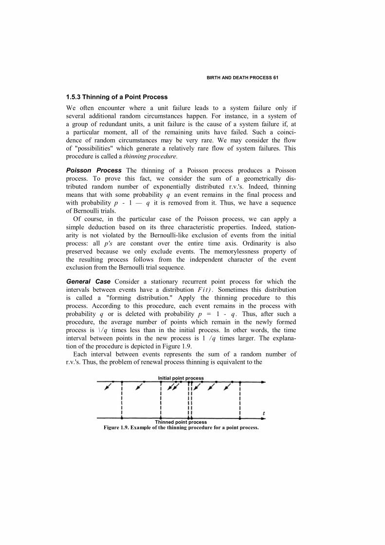
BIRTH AND DEATH PROCESS 61
1.5.3 Thinning of a Point Process We often encounter where a unit failure leads to a system failure only if several additional random circumstances happen. For instance, in a system of a group of redundant units, a unit failure is the cause of a system failure if, at a particular moment, all of the remaining units have failed. Such a coinci- dence of random circumstances may be very rare. We may consider the flow of "possibilities" which generate a relatively rare flow of system failures. This procedure is called a thinning procedure.
Poisson Process The thinning of a Poisson process produces a Poisson process. To prove this fact, we consider the sum of a geometrically dis- tributed random number of exponentially distributed r.v.'s. Indeed, thinning means that with some probability q an event remains in the final process and with probability p - 1 — q it is removed from it. Thus, we have a sequence of Bernoulli trials.
Of course, in the particular case of the Poisson process, we can apply a simple deduction based on its three characteristic properties. Indeed, station- arity is not violated by the Bernoulli-like exclusion of events from the initial process: all p's are constant over the entire time axis. Ordinarity is also preserved because we only exclude events. The memorylessness property of the resulting process follows from the independent character of the event exclusion from the Bernoulli trial sequence.
General Case Consider a stationary recurrent point process for which the intervals between events have a distribution F i t ) . Sometimes this distribution is called a "forming distribution." Apply the thinning procedure to this process. According to this procedure, each event remains in the process with probability q or is deleted with probability p = 1 - q . Thus, after such a procedure, the average number of points which remain in the newly formed process is \ / q times less than in the initial process. In other words, the time interval between points in the new process is 1 / q times larger. The explana- tion of the procedure is depicted in Figure 1.9.
Each interval between events represents the sum of a random number of r.v.'s. Thus, the problem of renewal process thinning is equivalent to the
Initial point process
Thinned point process Figure 1.9. Example of the thinning procedure for a point process.
62 FUNDAMENTALS
summation of a geometrically distributed random number of r.v.'s. (This was considered in Section 1.4.) In particular, in Section 1.4.5 we developed some asymptotic results. Here we use the standard terminology and methods of renewal theory, because this helps us to obtain some additional results.
Consider a special transformation of the renewal process, Tq: events are deleted from the process with probability p , and, simultaneously, the time scale is shrinking by a factor of \ / q . This normalization of time keeps the length of the average interarrival interval the same as in the initial process. It is clear that the TQ transformation is equivalent to the summation of a geometrically distributed random number of r.v.'s with a d.f. F i t ) and the further normalization of the resulting r.v.
Sequential applications of the transformations TQ and TQI to the process are equivalent to the single transformation TQ . We ask the reader to prove this is Exercises 1.11 and 1.12.
Limit R&nyi Theorem The Renyi theorem is very important in many applications. These asymptotic results can be used if the thinning procedure is intensive enough. They are also very useful in developing heuristic ap- proaches (see Chapter 13).
Theorem 1.6 If transformations TQI, TQ ,.,., are such that, for n -* «>,
Qn = Q \ d 2 •*•«„-» 0 as n -> 0
then their application to some point renewal process with an initial finite intensity A leads the resulting limit process to a Poisson process with the same intensity A.
We omit the proof because, in general, it coincides with the corresponding proof of Section 1.3.5.
Later this result was generalized for the superposition of n different renewal processes with different thinning procedures.
We remark that a Poisson process is sometimes called "a process of rare events." From formulations of the above results, one can see that the TQ transformation generates the flow of "rare" events from a dense initial process.
1.5.4 Superposition of Point Processes In reliability practice we frequently encounter a situation which might be described as the formation of a common point process from the superposi- tion of several point processes (see Figure 1.10).
For example, consider the flow of failures of different units in a series system. Each unit generates its own renewal point process of failures: a failed
BIRTH AND DEATH PROCESS 63
Resulting point process Figure 1.10. Example of the
superposition of two point processes.
unit is replaced and the process continues. Unfortunately, even if we con- sider a small number of renewal processes, their superposition cannot be analyzed in terms of renewal processes! (The only exception is the superposi- tion of Poisson processes.)
At the same time, fortunately, if the number of superimposed point processes is very large, the superposition of these processes produces a point process that is very close to being Poisson. In the theory of stochastic processes, the Poisson process plays a role which is analogous to that of the normal distribution in probability theory.
Poisson Process For the superposition of n Poisson processes, the result- ing process is Poissonian. If the initial processes have parameters Ap A2,..,, An, the resulting process has the parameter AL = £Ar To show this fact, consider an arbitrary moment of time t . Let (k denote the residual time of the kth process, that is, the time from an arbitrary but fixed t until the appearance of the next event in the process. The memoryless property says that two r.v.'s £k and £k, which represent the time between events for the A th process, are statistically equivalent. Thus, for the &th initial process we can write the distribution of the residual time
Pr{^ >/} = Pr{^>r} -exp(-Ar).
If we consider n processes, then, from a fixed (albeit arbitrary) moment t until the next arriving event, we observe an r.v.
U « tnin ik 1 ^k<.n
with d.f.
Pr{& ^ t } = Pr{ min {k > A \ ] £ k < n >
- n n e-**'-exp( ~ t £ A , 1 Stin litiii A
First process" Second, process
TT t I
i i t g t i
t i i i i
-4—1—4-
-4—4-

64 FUNDAMENTALS
Thus, the distribution of the time interval between neighboring events is exponential. As we know, only the Poisson process is characterized by such a property.
Of course, as above, we can prove this fact by checking that all three characteristic properties of the Poisson process are satisfied. Indeed, station- arity is kept because of the stationarity of all initial processes. Ordinarily is also preserved, because, for a continuous process, the probability of a coincidence of events equals 0. The memorylessness property of the resulting process follows from the independence of all the initial processes and their original memorylessness property.
General Case The proofs and even the formulation of the strict conditions of the related theorems are complex and lie outside the scope of this book. We only formulate the main results, sometimes even on a verbal level. The first strict result was formulated in the following theorem.
Khinchine- Ososkov Theorem If the limit
Iim £ Anr = A
exists, a necessary and sufficient condition that the process Jr„{r) converges to a Poisson process with parameter A is that, for any fixed t and n - >
Later general results, relating to the superposition of stochastic point processes, are contained in the Grigelionis-Pogozhev theorem. On a qualita- tive level, the theorem states that a limit point process which is formed by the superposition of independent "infinitesimally rare" point processes converges to a Poisson process. The parameter of this resulting process is expressed as a sum of the parameters of the initial processes.
1.6 BIRTH AND DEATH PROCESS
The birth and death process is an important branch of Markov processes. We will not give details for the general Markov processes, but we will consider some special models of renewal systems in a later chaptcr. This approach is also very useful for the analysis of renewal systems.
1.6.1 Model Description The behavior of a number of practical systems can be portrayed with the help of the birth and death process (BDP). Birth and death processes are widely
BIRTH AND DEATH PROCESS 65
used for the construction of mathematical models in microbiology, zoology, and demography. They are also used in reliability and queuing theory.
Let us explain the nature of the BDP with three simple examples. Consider a queueing system with one service unit and an unlimited number
of input call sources. Suppose there are k calls on the line waiting for service at a moment t . We say that at this moment, the system is in state H k . At the moment t + A t , where At is infinitesimally small, the state changes to H k + ] if an additional call arrives during the interval A t . If during A t a call service in the system has been completed, at the moment / + Afthe system changes its state to Hk_v Recall that, for a Markov process, the probability of more than one state change is o ( A t ) , which means that o(At) 0 as A t -» 0. From our assumption of an unlimited number of input sources of calls, it follows the line length could be infinite. In other words, a BDP may have an infinite number of states. Suppose there is a specified criterion of system effectiveness; for example, a line of length more than m is considered to be inadmissible. Then the set of all system states may be divided into two subsets: the "up states" H 0 , , . . , H m and the "down states" H m + 1, H m + 2 , . . . .
As another example, consider a parallel system with one main unit and m identical active redundant units. There is one repair facility. This system may be thought of as a queuing system with a limited number (namely, n + 1) of input "call" sources. Indeed, if there are k units under repair, then only m + 1 - k of the remaining units may fail. The state Hm + i corresponds to system failure, and only a transition from this state to state H m is possible. State Hm +, is called reflecting.
As the final example, consider a parallel system with n main units and m identical active redundant units. Again, there is one repair facility. It is clear that the mathematical description of this system is very close to that of the above example. In this case there are, in total, n + m sources of failure. The states H m + U . . . , Hn+m correspond to system failure states.
The last two examples are of BDPs with a finite number of states. In reliability theory it is sometimes reasonable to consider separately these two very similar cases.
The transition graphs for all three examples are shown in Figure 1.11. If the system is in state Hj at a moment t , there are three possibilities
during the next interval A t :
' The process passes to state Hj+X with probability: A, A t + o ( Ar)
• The process passes to state H J _ 1 with probability: M j A t + o ( A t )
• The process remains in state Hj with probability: 1 - ( A y + M j ) A t + o ( A t )
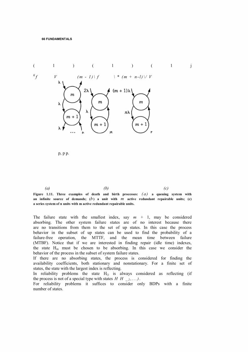
66 FUNDAMENTALS
( 1 ) ( 1 ) ( 1 j
K f V ( m - 1 ) \ f \ * ( m + n - l ) \ / V
p, |JL P
p, p p.
(a) (b) (c) Figure 1.11. Three examples of death and birth processes: ( a ) a queuing system with an infinite source of demands; (b ) a unit with m active redundant repairable units; (c) a series system of n units with m active redundant repairable units.
The failure state with the smallest index, say m + 1, may be considered absorbing. The other system failure states are of no interest because there are no transitions from them to the set of up states. In this case the process behavior in the subset of up states can be used to find the probability of a failure-free operation, the MTTF, and the mean time between failure (MTBF). Notice that if we are interested in finding repair (idle time) indexes, the state Hm must be chosen to be absorbing. In this case we consider the behavior of the process in the subset of system failure states. If there are no absorbing states, the process is considered for finding the availability coefficients, both stationary and nonstationary. For a finite set of states, the state with the largest index is reflecting. In reliability problems the state H() is always considered as reflecting (if the process is not of a special type with states H H _ 2 , . . . ) . For reliability problems it suffices to consider only BDPs with a finite number of states.

BIRTH AND DEATH PROCESS 67
1.6.2 Stationary Probabilities Consider a finite BDP with N + 1 states (see Figure l.lltr). For each state K and for two infinitesimally close time moments t and ( + A t , we can write
68 FUNDAMENTALS
the expression
p k ( t + A t ) =p*_,(0[A*_, Af +o(A0]
+ M')[1 - (A* + Mk) A/ + o(Ai)]
+ +o(A/)] + o ( t )
p k ( t + A O ~ p k ( t ) - - - - - - - - - - - - - - - - - - A k - i P k - i ( t ) ~ ( A * + M k ) p k ( t ) + M k + i p k + i ( t )
In the limit as A / -» 0, we obtain
p k ( t + A t ) - p k ( t ) hm ------------ — ---------- = />'(/) At >0 A t
- Ak - i Pk - i O ) - (Ai +Mjt)pA(r) + M*+1/>*+.(0 (1.112)
Because we are considering a finite process, we must set A_, = Af„ = AN = , = 0. In other words,
P'oiO = "A0Po(0
and
^(0 = -A„_,pw_,(f) + MN/7N(r)
We add to this system of equations the normalizing equation L pk(0 - i 0<:/<;JV
and exclude any one of the above. We note that (1.112) represents the equation of dynamic equilibrium. In other words, state k "loses each unit of its mass" p k ( t ) with intensity A k + M k and "receives" a corresponding mass from states k - 1 and k + 1. If there is no absorbing state, the process has stationary states. Thus, there are limits
lim P k ( t ) = p k
Moreover, if for any k ,
(1.113)
the stationary probabilities of these states do not depend on the initial state
BIRTH AND DEATH PROCESS 69
at t = 0. The condition (1.113) means that there are no separated groups of states. Consider this stationary case. If we take the limit as ; -* <x> in (1.112), we obtain the system of linear equations
0 = -A 0p0 + M i p 1
0 - A k - i Pk - i - ( A k + M k ) Pk + M k + l p k + ] (1U4)
0 = -A N - t p N + ] + M N p N .
Wc again must replace one of the above equations with the normalizing condition
E P* = l {1-H5)
Now let us recall that (1.114) represents an equilibrium. It means that if we consider any cut in the transition graph, for instance, a cut between states k - 1 and k , there is an equality of flows "up" and "down":
M k p k = A . k _ ] p k _ l (1.116)
From (1.116) we obtain the recurrent relationship A*-1
Pk=~j^-Pk-1 (1-117)
which allows us to obtain
Aq AJ . . . . . A A _ t Pk = ......... =7 Po - A k P o (1.118)
M,M2 ............ Mk
From (1.115) it follows that
n A, O z j z k - 1
n ^ ^k l z j z k
-------------------- TTT (,119) 0 rZj^N £ OS'S/-!
<wsAf n M. 1 SiS/
where A 0 = 1 .
1.6.3 Stationary Mean Time of Being in a Subset Consider a BDP whose total set of n states is divided into two subsets; one subset of up states, E+= {//„,..., H m ) , and another of down states, E.,=
+1> - - - * Hn}.
70 FUNDAMENTALS
To find the stationary mean time of the process present in a specified subset of states, we use a well-known result. Let us distinguish two subsets of so-called boundary states: e + which is a subset of E+ and e _ which is a subset of E_. The process may enter the subset leaving only a state belonging to the boundary subset e+. The subset e_ plays an analogous role for the subset E + . In considering case e + consists of only one state H m , Briefly repeat the idea of the conclusion. The process may leave subset E+ only from state H m , and being in this state it leaves with intensity A*. Hence, the intensity of leaving subset £+ equals
A + «P * A m (1.120) where p * is the conditional probability that the process is in state H m under the condition that this is in subset E+:
Pm Pl =
L Pj 0 s j s m
where p ) can be found from (1.119). Finally, we find that the mean stationary time of the process being in subset E + is T+= 1/A+:
r+= = (1.121) A m P m
Obviously, the mean stationary time of the process being in subset E _ is similar to the above except for the following notation:
A/_=A/m+,/>**-! where
m + 1
£ />, m +1
and, finally, E *
r _ - ( 1 . 1 2 2)
M m + i p m + l
1.6.4 Probability of Being in a Given Subset The BDP with an absorbing state Hn + ] can be described with the help of the following system of differential equations: d "/>(/) = A ~ ( A y + M j ) p j ( t ) + M j + i P j + i ( t ) O s / ^ n
+ 1
E />;(<) = 1 (1.123) 1
A_ i = A„ + 1 = M0 = A/„ + 1 = Mn + 2 = 0
P m+ I
BIRTH AND DEATH PROCESS 71
where p } ( t ) is the probability of state H j at moment t . Let the probabilities Pj(t) satisfy the initial conditions:
Pj { * ~ 0) =p,(0) 0 < j < n + l
Let 0 n + l be the duration of time before the system has reached the absorbing state Hn+l for the first time. We need to find the distribution function Pr{0„ + 1 ^ /} = pn + ,(f). This is the probability that the system has not reached the absorbing state Hn + i at time t. Let us apply the LST to (1.123). Then we find the system of linear algebraic equations:
A - ( A ; . + M j + + AJ + l 9 J + l ( s ) = -/>y(0) 0 5 < n + 1
Ay_, = A„ + 1 = M0 = Mn+l = Mn + 2 = 0 (1.125)
By using Cramer's rule,
(1.126)
where
(1.124)
72 FUNDAMENTALS
(1.128)
Expanding the determinant £>„ + ,(s) along the last row yields the recurrent
- (A0 + ») M, 0 0 0
A« — (A| + A/| + J) M2 0 0
= 0 A| -(AJ+A/J+J) 0 0
0 0 0 1+H,- , + S) M „
0 0 0 AN-. -(A n + M n
+ s )
(- -1)" +
1
n (s + x " k + l )
(1.127)
1 £ k < .
n +1
( s )
-(A„ + I) M, 0 0 0 - P<|(0) A«
-(A + M, + S) M2 0 0
0 A, -(A 2 + M 2 + S ) 0 0 - P2(0)
0 0 0 • -<A„_ , + M n
-1 +
S) M „ - Pn -,(0
) 0 0 0 A.-L ~(A„ + M„ - P„(0) 0 0 0 0 A» -P„+|(0)

BIRTH AND DEATH PROCESS 73
equation:
A,+,(*) = -P„+|<0) E (-i)n+ Pi(0) A((j) n \k (1.129)
The probability p„ + ,(f) is found with the help of the inverse LST:
1 , 1 , D n + l ( s ) e s ' d s P . . M - J S I S - . M ' " * - n l - . a . » , ( . ) ( , 1 3 0 )
where i = / — 1.
We are now faced with the problem of calculating the roots (eigenvalues) of (1.130). It can be shown that An + 1(s) is a polynomial of power n , and all of its roots + 1 < k < , n + 1, are distinct and negative. Also, all roots of the polynomials of the neighboring orders n and n + 1 are intermittent. This fact facilitates the computation of the recurrent equation (1.130). We omit the cumbersome intermediate transformations and write the final result, taking into account that the probability of interest P ( t ) = 1 - p n + l ( t ) :
P{ t ) - E p,(0) n A, E V r O n i z n t & j s n i s k & n + 1
1 £ i £ n i + k
In (1.131) we need to insert the roots which are usually calculated by numerical methods. Two cases are of special interest. They are given without special explana- tions:
1. When all units are in up states at moment t — 0. 2. When the system has just come out of a failure state at r = 0.
If the system begins its operation at the state with all units completely operational:
po(0) = 1 p,(0) =0 1 < i < n + 1
74 FUNDAMENTALS
then
/>«»(<) = A0A, ... A„ Z e , , n + i ) _ , n + i)) (1.132) im n + l S i 1 1 \ S k s i ) 1 + t k + i
If the system begins its operation just after coming out of a failure state.
P„(0) = 1 p , ( 0 ) = 0 i = 0 , 1 , . . . , / 2 - \ , n + 1 then
p<">(/> = (-ox z ' n (4"+ , )-*r , )) lsUsn + l S
> 1 1 1 k +i
(1.133)
1.6.5 Mean Time of Staying in a Given Subset Now let us determine the mean time of the process staying in the subset £ + = { / / „ , . . . , H m ) starting from the state H0. Of course, we may use a standard procedure for calculating this value: first, find the probability of staying in this subset with the initial condition H0(0) = 1 and then integrate the obtained expression. But this approach is too difficult. (Also, we did not obtain the result in a form which is easily integrated!) Thus, we choose another method. A transition of the process from the initial state H0 to the absorbing state H n + , can be considered as consisting of n + 1 steps:
2 from H{) to Hu plus • from //, to H2 (with the probability of going back and forth to the state //o), plus • from H 2 to H i (with the possibility of going back and forth to the states H0 and //,), plus
• from Hn to Hn + l.
Let us find the mean time of passing from Hk to Hk + ] where k > 0. Consider the auxiliary BDP with only k + 1 states where Hk+, is absorbing. We can use the stationary mean time of entrance in the absorbing state
BIRTH AND DEATH PROCESS 75
found in (1.131). Thus, the value of interest can be found to be
L A- T — V T — V ^fc / n , n + ] ~ Z-T * k , k + \ L i .
0 sitsn O s k s m a k Pk
1.6.6 Stationary Probability of Being in a Given Subset Let us again consider two subsets, E+ = {H0, , . , , Hm} and E_ = [Hm+ One can find the stationary probability of being in a given subset, say E+, in two ways. Denote this probability K. The first way amounts to finding
A: = lim Pr{tfy(r) e£ + } = £ Pj
The second way uses the means T + and T_ determined in (1.121) and (1.122), respectively. Let K - 1 = k . For the stationary process, the probabil- ity of being in a given state is proportional to the portion of time occupied by this state over the entire interval of observation on the time axis. This leads to the condition ( K / k ) = ( T + / T_ ). With the condition K + k = 1 we find
T +
1.6.7 Death Process A particular class of birth and death processes is the so-called death process. From the name of the process, it is clear that this can be obtained from the BDP by putting all M j , 1 < , j £ N , equal to 0. We consider this mathematical model because it is very useful when dealing with certain redundant systems without repair. For example, a redundant system consisting of n identical dependent units might be analyzed with this technique. The units can be dependent in a special way when the failure rate of each of them depends on the number of failed (or, equivalently, the number of operating) units at the moment. This process can be described by the linear transition graph (see Figure 1,12). Let the process have N + 1 states: H 0 , . . . , H N . Let A k denote the transition rate from state Hk to state Hk+t. Using the same technique as above, we can write the equation:
p'kU) - -Ak P k ( t ) + Ajt_,pA_i(r) (1.134)
for all 0 ^ k < N - 1 and A _, = \N = 0.
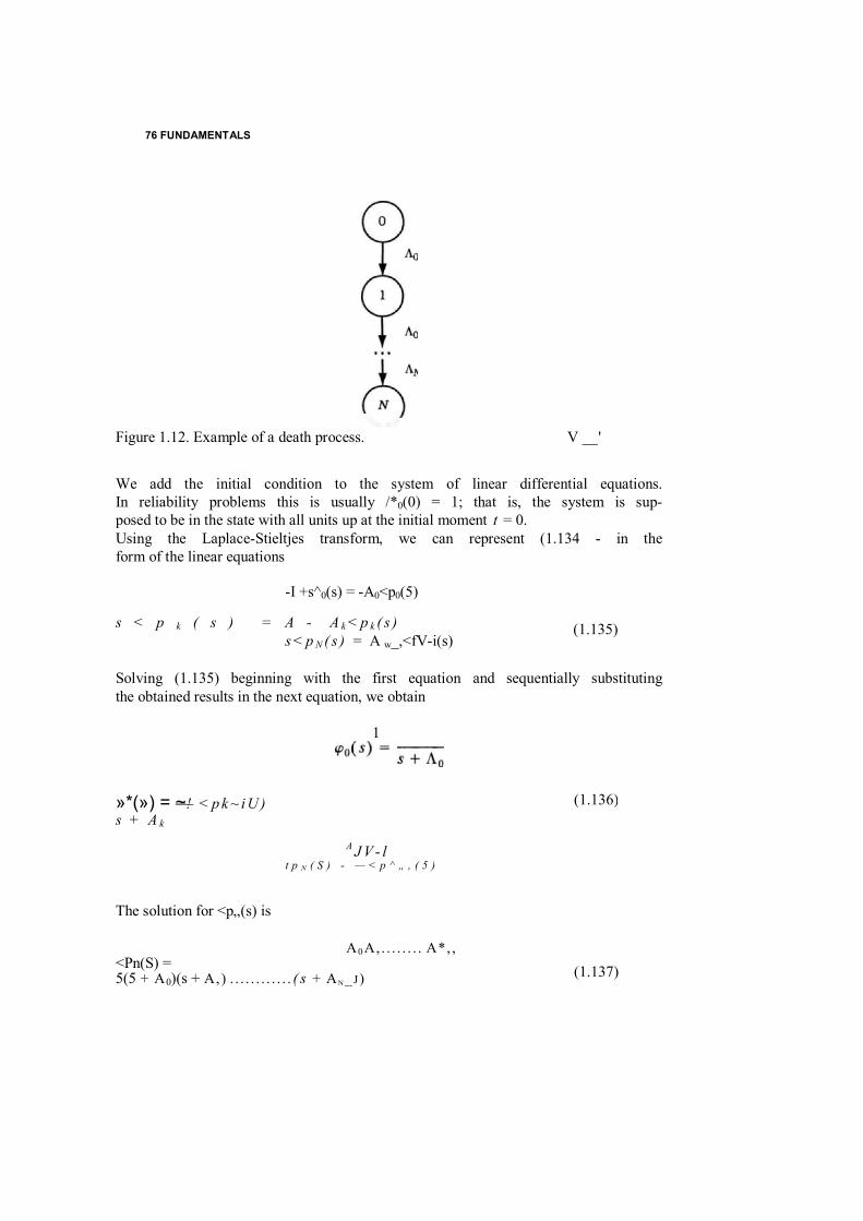
76 FUNDAMENTALS
Figure 1.12. Example of a death process. V __ '
We add the initial condition to the system of linear differential equations. In reliability problems this is usually /*0(0) = 1; that is, the system is sup- posed to be in the state with all units up at the initial moment t = 0. Using the Laplace-Stieltjes transform, we can represent (1.134 - in the form of the linear equations
-I +s^0(s) = -A0<p0(5)
s < p k ( s ) = A - A k < p k ( s ) s < p N ( s ) = A w_,<fV-i(s)
Solving (1.135) beginning with the first equation and sequentially substituting the obtained results in the next equation, we obtain
1
»*(») = ~! < p k ~ i U ) s + A k
A J V - l t p N ( S ) - — < p ^ „ , ( 5 )
The solution for <p„(s) is
A0 A,. . . . . . . . A*, , <Pn(S) = 5(5 + A0)(s + A,) . . . . . . . . . . . . ( s + AN_ J)
(1.135)
(1.136)
(1.137)
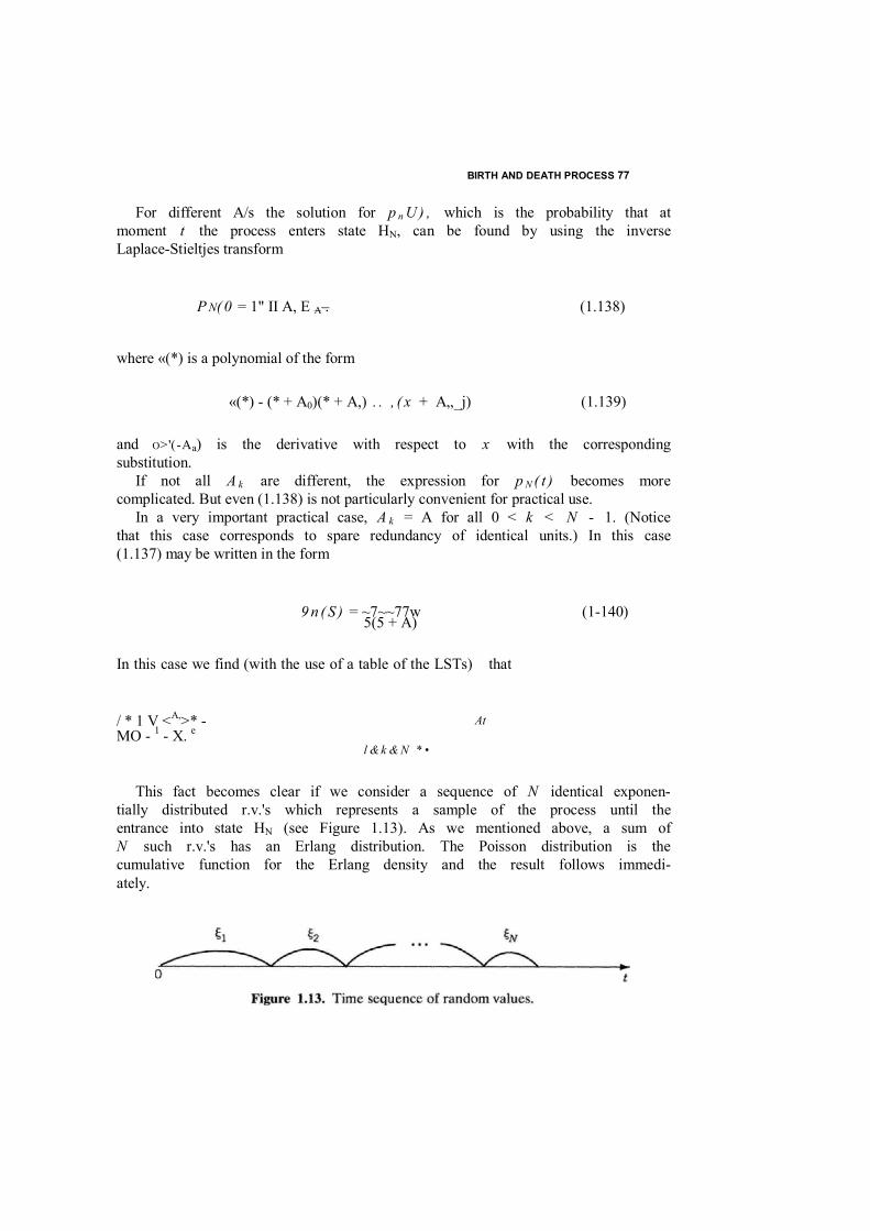
BIRTH AND DEATH PROCESS 77
For different A/s the solution for p n U ) , which is the probability that at moment t the process enters state HN, can be found by using the inverse Laplace-Stieltjes transform
P N( 0 = 1" II A, E A . (1.138)
where «(*) is a polynomial of the form
«(*) - (* + A0)(* + A,) . . , ( x + A„_j) (1.139)
and O>'(-Aa) is the derivative with respect to x with the corresponding substitution.
If not all A k are different, the expression for p N ( t ) becomes more complicated. But even (1.138) is not particularly convenient for practical use.
In a very important practical case, A k = A for all 0 < k < N - 1. (Notice that this case corresponds to spare redundancy of identical units.) In this case (1.137) may be written in the form
9 n ( S ) = ~7~~77w (1-140) 5(5 + A)
In this case we find (with the use of a table of the LSTs) that
/ * 1 V <A,>* - MO - 1 - X. e
l & k & N * •
This fact becomes clear if we consider a sequence of N identical exponen- tially distributed r.v.'s which represents a sample of the process until the entrance into state HN (see Figure 1.13). As we mentioned above, a sum of N such r.v.'s has an Erlang distribution. The Poisson distribution is the cumulative function for the Erlang density and the result follows immedi- ately.
At
78 FUNDAMENTALS
The mean time of the process entering into state H N in the general case can easily be calculated as the sum of the time periods during which the process is remaining in each state
N ~ ~T~ 1 < , k < , N
Some details concerning death processes will be discussed later.
CONCLUSION
Two distributions which are often used in engineering practice are the normal and the exponential. Each has its advantages and disadvantages. First of all, these distributions are very convenient for varied mathematical manip- ulations. But this argument is weak for practical applications. The question of their reasonable use, as with any modeling of real objects with the help of mathematical abstraction, always requires special "physical" verification based on experience and engineering intuition.
A Weibull-Gnedenko distribution is very convenient as a model for various physical phenomena because it is two parametrical. Besides, it has a clear physical sense as a distribution of extremal values. This distribution, as it relates to applied mechanical problems, was first mentioned in Weibull (1939). shortly after this, Gnedenko (1943) found classes of limit distributions of extreme values. A particular type of limit distribution has the form of the distribution discovered by Weibull
F( t ) = 1- ~ exp | - exp | J J where the new parameters are expressed as b = 1/0 and a - log A.
The reader interested in a deeper understanding of the probabilistic fundamentals of reliability theory should pay attention to special mono- graphs. It is practically impossible to enumerate the books dedicated to this subject. An older, but nevertheless highly recommended book, is the book by Feller (1966). This book along with the book by Gnedenko (1967, 1988) were the main textbooks for several generations of statisticians and applied mathe- maticians.
For everyday use the books by DeGroot (1987) and Devore (1991) are recommended.
Concerning the limit theorems in the theory of stochastic processes, we must especially mention several works. Khinchine (1956a, 1956b, 1960) and Ososkov (1956) considered superposition of point processes, and later Grige- lionis (1963) and Pogozhev (1964) generalized their result. Renyi (1962)
REFERENCES 79
formulated the theorem on "thinning" of point processes which later was generalized by Belyaev (1962). Summary of all of these results can be found in Gnedenko and Kovalenko (1987). The reader can find details concerning generalized generating sequences in Ushakov (1986, 1987, 1988a, 1988b).
REFERENCES
Belyaev, Yu. K. (1962). Line Markov processes and their application to problems in reliability theory. Trans. Sixth Conf. Probab. Statist., Vilnius. DeGroot, M. H. (1987). Probability and Statistics, 2nd ed. Reading, MA: Addison- Wesley. Devore, J. L. (1991). Probability and Statistics for Engineering and the Sciences, 3rd ed. Pacific Grove, CA: Brooks/Cole. Feller, W. (1966). An Introduction to Probability Theory and Its Applications. New York: Wiley. Gnedenko, B. V. (1943). Sur la distribution limit du termc maximum d'une scrie aleatoir. Ann. Math., no. 44. Gnedenko, B. V. (1967). The Theory of Probability. New York. Chelsea. Gnedenko, B, V., Kovalenko, I. N. (1987). Introduction in Queuing Theory, 2nd ed. (in Russian). Moscow: Nauka. Gnedenko, B. V. (1988). Course of Probability Theory, 6th ed., revised (in Russian). Moscow: Nauka. Grigelionis, B. (1963). On the convergence of sums of step stochastic processes to a Poisson process. Theory Probab. Appl., vol. 8, no. 2. Grigelionis, B. (1964). Limit theorems on sum of renewal processes. In Cybernetics in the Service of Communism, vol. 2, A. Berg, N. Bruevich, and B. Gnedenko, eds. Moscow: Energia. Khinchine, A. Ya. (1956a). Streams of random events without aftereffect. Theory Probab. Appl., No. 1. Khinchine, A. Ya. (1956b). On Poisson streams of random events. Theory Probab. Appl., no. 1. Khinchine, A. Ya. (I960). Mathematical Methods in the Theory of Queueing. London: Charles Griffin. Ososkov, G. A. (1956). A limit theorem for flows of similar events. Theory Probab. Appl., vol. 1, no. 2. Pogozhev, I. B. (1964). Evaluation of deviation of the equipment failure flow from a Poisson process. In Cybernetics in the Service of Communism, vol. 2, (in Russian) A. Berg, N. Brucvich, and B. Gnedenko, eds. Moscow: Energia. Renyi. A. (1956), Poisson-folyamat egy jemllemzese (in Hungarian). Ann. Math. Statist., vol. 1, no. 4. Renyi (1962). Ushakov, I. A. (1986). A universal generating function. Soviet J. Comput. Systems Sci., vol. 24, no. 5.
80 FUNDAMENTALS
Ushakov, I. A. (1987). Optimal standby problem and a universal generating function. Soviet J. Comput. Systems Sci., vol. 25, no. 4. Ushakov, I. A. (1988a). Reliability analysis of multi-state systems by means of a modified generating function. J. Inform. Process. Cybernet., vol. 24, no. 3. Ushakov, I. A. (1988b). Solving of optimal redundancy problem by means of a generalized generating function. J. Inform. Process. Cybernet., vol, 24, no. 4-5. Weibull, W. (1939). A statistical theory of the strength of materials. I n g . Vetenskaps Akad. Handl., no. 151. Weibull, W. (1951). A statistical distribution of wide applicability. J. Appt. Mech., no. 18.
APPENDIX: AUXILIARY TOOLS
1.A.1 Generating Functions
Let v be a discrete random variable (r.v.) with distribution
p r { ! / = k } k « 0 , 1 , 2 , . . .
L Pk -1 V k
The generating function (g.f.) of v denoted by < p ( z ) is defined as
<PU) ~ Y ,PkZk V k
Thus, the coefficient of z k equals the probability that v equals k . The g.f. is very convenient when one deals with the summation of discrete r.v.'s. Generating functions are especially effective when algorithms for computer calculations are involved. For example, suppose we have two discrete r.v.'s a and (i, with distribu- tions a k and b k , respectively. We are interested in the distribution g k of the new r.v. y = a + f3. Of course, we could find the desired distribution directly:
pr{r = m pr{« = 0} Pr{/3 = + Pr{a = 1} Pr{0 = k - 1}
+ ... +pr{« = 4} Pr{/3 = 0} = Z a j b k - j = Z " k - j b j ( 1 1 4 1 )
0 <j<.k 0
But such an approach is not always simple or convenient. For computational purposes it is often better to use the g.f.'s of a and f3. Let < p a ( z ) , 0p(.z), and < P y ( z ) be the g.f.'s of the respective distributions. Then we have
#,(*) = < P a ( z ) < Pf > ( z )
APPENDIX: AUXILIARY TOOLS 81
In the new polynomial the coefficient of z k is automatically equal to expression (1.141). This example does not exhibit all of the advantages of generating functions, but below we will show other cases where the use of g.f.'s is very effective. Suppose we wish to find PT { V £ k ) . We note that
Pr{i/ <; k } =
z - 0
where M i - o ^ operator that turns any negative power t of the term z ' into 1. Thus, after the substitution z = 0,
Pr{y < A:} = £ P k
Furthermore, it is clear that
d
E * p k z k - * z- I
= E * P k = E {v ] z - 1
To obtain higher moments, it is more convenient to use the
so-called moment generating function (m.g.f.) < p ( s ) of the r.v. v . This function can be written formally by simply substituting 2 = e s into the generating function, that is, < p ( e s ) - < f > ( z ) . Then
E k *p k e* 1 = E = = VJt2t 1 Ji-o VJtal
1 .A.2 Laplace - Stieltjes Transformation With continuous r.v.'s the Laplace-Stieltjes transformation (LST) is often used. This transformation allows one to solve integral-differential equations with the "reduced" mathematical technique. The essence of the LST is depicted in Figure 1.14. In this book we usually consider distributions of nonnegative r.v.'s. The transforms of such r.v.'s are defined for the distribution function (d.f.) F i t ) as
< p F ( s ) = [ ~ F( t ) e — d t J a
1: < P( Z )
dz
= ' E kpke'k
5 — 0 .v/ra 1 = E kp k = E{v ]
r-0 VAa l
d
J -O ds ds
d_2
ds
= m(2)2 < P( e s )
j = 0
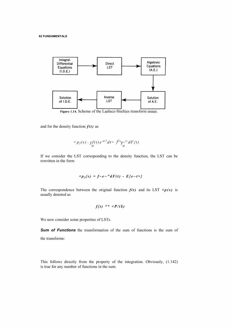
82 FUNDAMENTALS
and for the density function f i t ) as
< p f ( s ) = r f ( t ) e " s l d t = fC°e~s' d F{ t ) J o J o
If we consider the LST corresponding to the density function, the LST can be rewritten in the form
< p f { s ) = f ~ e ~ " d F( t ) - E{ e ~ t > }
The correspondence between the original function f i t ) and its LST < p ( s ) is usually denoted as
f { t ) * * < P / i $ )
We now consider some properties of LSTs.
Sum of Functions the transformation of the sum of functions is the sum of
the transforms:
This follows directly from the property of the integration. Obviously, (1.142) is true for any number of functions in the sum.
Figure 1.14. Scheme of the Laplace-Stieltjes transform usage.
APPENDIX: AUXILIARY TOOLS 83
Convolution of Functions The convolution of two functions /}(t) and f 2 ( t ) is the function f i t ) defined by
A0 = j ' f y ( t - x ) f 2 ( x ) dx ~ f f 2 ( t - x ) f l ( x ) dx J o J o
This operation over the functions /,(/) and f 2 i t ) is also denoted by
AO ■ /i * A(0 The transform of the convolution of a pair of functions is the product of the transforms:
/i*/2(0 <Pj(s)<M5)
The proof of this is left as Exercise 1,14. Obviously, the correspondence is true for any number of functions in the convolution:
f l * f i * ■ ■ ■ * W ) ( s ) - - - 9 n ( s )
Derivative of a Function The transform of the derivative of a function can be expressed in terms of the transform of the function as
no «♦**>(*) - A®) The proof of this is left as Exercise 1.15.
Integral of a Function The transform of the integral of a function can be expressed by the transform of the function as
f ' f ( t ) d t ~ J n X J 0 S
The proof of this is left as Exercise 1.16.
Property of the LST of the Density Function If the function /(/) is the density of the distribution of the r.v. that is, f i t ) = [ d Fi t ) ] / d t , then
/ AO' J n
and
= - / V t o * = - m)
J n
(1.143)
(1.144)
(1.145)
d t (1.146)
.'ns - 0
~/V(o< J n d t S-0

84 FUNDAMENTALS
Property of the LST of the PFFO If P i t ) is the probability of a failure-free operation, that is, P i t ) ~ 1 - F i t ) , then the corresponding LST at 0 is
r p ( t ) e ~ s , d t = f "p ( t ) d t = T J 0 Jj».o Jo
where T is the mean of the distribution F i t ) — 1 — Pi t ) . This value is called the mean time to failure (MTTF).
Initial Moments of a Distribution The Laplace-Stieltjes transformation of the density function allows us to obtain the moments as
(1.148)
These moments are obtained more conveniently with the help of the continu- ous m.g.f. which coincides with the LST except in the sign of the power in the exponential:
- r f ( t ) e s ' d t J i i
In this case there is no change in the sign:
ds* s—o
The Laplace-Stieltjes transformation represents a very useful mapping from one functional space into a new one where the original functions are replaced with transformed ones. Operations over these new functions are often simpler in the transformed space. The general idea is reflected in Figure 1.14,
1.A.3 Generalized Generating Sequences The method of generalized generating sequences (GGS) is based on a new approach which is genetically tied to generating functions. It is very conve- nient for a computerized realization of different enumeration problems which often arise in discrete optimization. We begin with a simple example to illustrate the main features of the GGS. Consider a series connection of n resistors. Each unit in the series has a resistance which has a random value (for various reasons, e.g., manufactur- ing, storage, environmental influence, etc.). This random value of the unit's
(1.147)
d k
ds*
s - 0
APPENDIX: AUXILIARY TOOLS 85
resistance is characterized by some distribution. We assume that this distri- bution is discrete and the resistance of the ith resistor equals the value ru with probability p(}, so that
L Pa = 1 I Z / S M ,
where M, is the number of discrete values of the ith resistor. For each unit we can construct the generating function of the distribution of the resistance values:
G ; ( Z ) = E PuZ'" 1 <,i<.M>
To find the distribution of the resistance of the entire series connection, we can compute its g.f.
G ( z ) = n <?/(*) = n L Pij*rii (1-149) \ s i s f 1 s i s n 1 s M j
After simple algebraic transformations, we write the final expression in the form of a polynomial
C ( z ) = £ P,zR- (1.150)
where the coefficient Ps of the term zR' equals the probability that the series system's resistance is Rv We remark that, in a computational sense, the introduction of the auxiliary variable z permits us to separate the variables of interest: p and r . (We omit other useful properties of the g.f. for this discussion because they are irrelevant here.) To compute P s and R s , one needs only to multiply the p 's and to add the r's. This example is very clear and contains no new information for those who know how to work with generating functions. Of course, if the problem is to calculate the resistance of a parallel connection of resistors, it is impossible to use (1.149) and (1.150) in any direct way. To use the g.f., one has to consider r.v.'s which measure conductivity (instead of resistance) and then find the desired result in terms of conductivity. Finally, the result can be transformed from units of conductivity to units of resistance. Now suppose it is necessary to analyze the pipeline capacity of a set of pipes connected in series. In this example the collective capacity is the minimum of the capacities of the individual units. The usual generating function does not work here at all! We suggest a new approach which we call the generalized generating sequence (GGS).
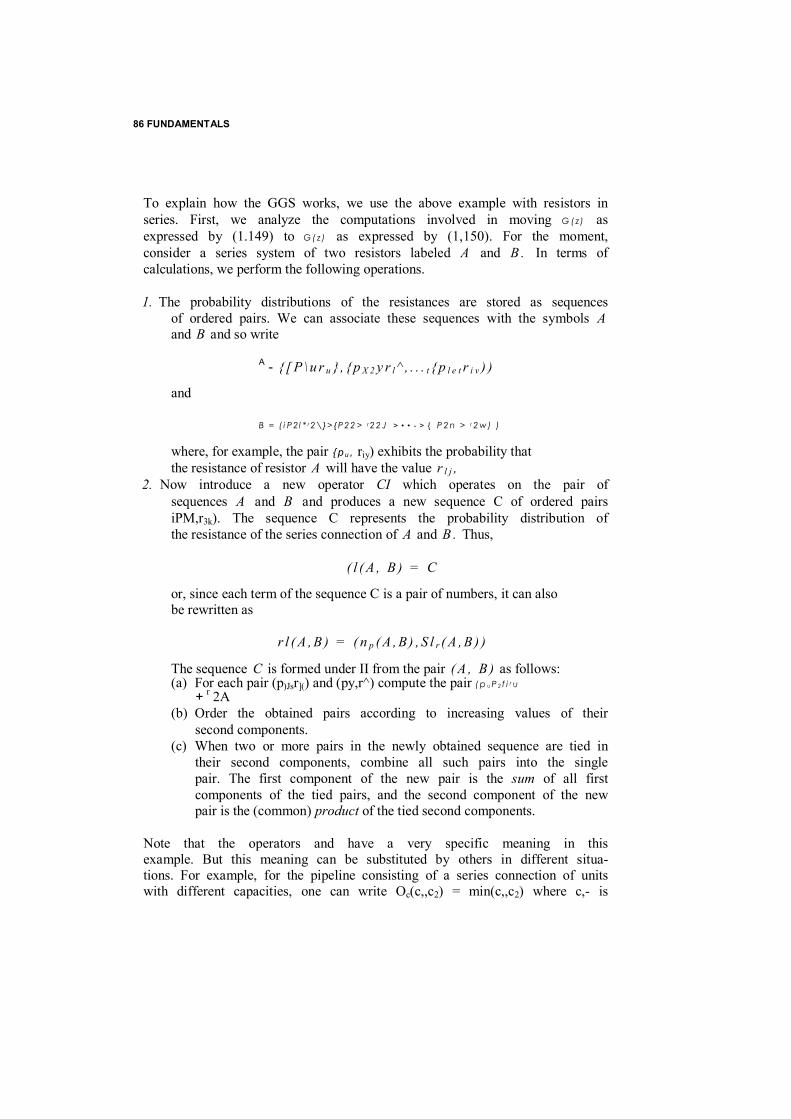
86 FUNDAMENTALS
To explain how the GGS works, we use the above example with resistors in series. First, we analyze the computations involved in moving G ( z ) as expressed by (1.149) to G ( z ) as expressed by (1,150). For the moment, consider a series system of two resistors labeled A and B . In terms of calculations, we perform the following operations.
1. The probability distributions of the resistances are stored as sequences of ordered pairs. We can associate these sequences with the symbols A and B and so write
A - { [ P \ u r u } , { p X 2 y r l ^ , . . . t { p l e t r i v ) )
and
B = ( i P 2 l * r 2 \}> {P 2 2 > r 2 2 J > • • - > { P 2 n > r 2 w) )
where, for example, the pair { p u , riy) exhibits the probability that the resistance of resistor A will have the value r l j ,
2. Now introduce a new operator CI which operates on the pair of sequences A and B and produces a new sequence C of ordered pairs iPM,r3k). The sequence C represents the probability distribution of the resistance of the series connection of A and B . Thus,
( l ( A , B ) = C
or, since each term of the sequence C is a pair of numbers, it can also be rewritten as
r l ( A , B ) = ( n p ( A , B) , S l r ( A , B ) )
The sequence C is formed under II from the pair ( A , B ) as follows: (a) For each pair (p)Jsr]() and (py,r^) compute the pair ( p u P 2 f i r u
+ r 2A (b) Order the obtained pairs according to increasing values of their
second components. (c) When two or more pairs in the newly obtained sequence are tied in
their second components, combine all such pairs into the single pair. The first component of the new pair is the sum of all first components of the tied pairs, and the second component of the new pair is the (common) product of the tied second components.
Note that the operators and have a very specific meaning in this example. But this meaning can be substituted by others in different situa- tions. For example, for the pipeline consisting of a series connection of units with different capacities, one can write Oc(c,,c2) = min(c,,c2) where c,- is
APPENDIX: AUXILIARY TOOLS 87
the capacity of the ith pipe. All of the remaining formal operations and the order of their performance are similar. Therefore, the above-described computational algorithm, in general, can be used with no restrictions on the polynomial form. The new approach can be used for enumeration problems involving different physical parameters. We will show the effectiveness of this operator for computational problems of complex system reliability analysis and discrete optimization problems.
Now let us describe the procedure in more general terms. Keeping in mind the use of a computer, we introduce a more formal description.
For a more vivid presentation we will use a special terminology to distin- guish the GGS from the g.f. This will relieve us of having to use traditional terms in a new sense, which often leads to confusion. Moreover, we hope that this new terminology can help us, in a mnemonical sense, to remember and even to explain the procedure.
In an ancient Roman army, a cohort was the main combat unit. Each cohort consisted of maniples which were independent and sometimes special- ized simple combat units. Several cohorts composed a legion. The use of this essentially military terminology appears to be convenient in this essentially peaceful applied mathematical field. We set up a one-to-one correspondence between the above-mentioned military units and the GGS with its attributes.
Consider a system consisting of n units. Each unit j is characterized by its GGS. Let the GGS of a unit be called a legion. Each legion j includes Vj cohorts:
Each cohort C j k is composed of some set of the unit's parameters, special characteristics, and auxiliary attributes. We call these components of the cohort maniples. Therefore,
CJ K = (M J K , , M J K 2 , . . . , M J V . S )
where M J l t is the corresponding maniple and s is the number of different maniples (assumed to be the same for each cohort).
The operation of interaction between legions is denoted by ClL. This operator is used to obtain the resulting legion
L = NL L ,
The operator ClL denotes a kind of "n-dimensional Cartesian product" and a special "reformatting" of the resulting cohorts. This reformatting depends on

88 FUNDAMENTALS
the specific nature of the problem [see, e.g., item (c) of the series resistors example]. As a result of this interaction of the legions, one obtains
N = N OJ 1
new cohorts. For each cohort the following notation is used where Clc
denotes the cohort's interaction, k is the subscript of this cohort in the set obtained as a result of the procedure
c, = nc ctl i
i ^ k
(before using the formatting procedure), and ij are corresponding subscripts of the cohorts taking part in the interaction (this fact is conditionally reflected in the notation ij ** k). The new cohort can be represented as
C k = ( M k X , M k 2 , . . . , M k s )
Each new cohort is obtained as a result of a vector product-type interac- tion of maniples: n maniples of the first type interact between themselves, n maniples of the second type interact between themselves, and so on. The interaction between maniples of a specified type can be called a "natural" interaction because they involve a real physical sense of the corresponding parameters:
- Of A%
1 i.efc
Here the subscript I defines the type of maniple interaction. The resulting legion consists of a set of cohorts obtained by using the formatting procedure. It can be written as
L = ( C j i j , C ( 2 ) , . . . ,
where N * < N . This formatting procedure can consist of special operations over N cohorts. For example, several cohorts can be joined into an equivalent one in which some specified maniple equals the sum of others: we have the same solution with the g,f. when we add the probabilities of the terms with the same power of z. It may also be the selection of a "priority" (or "domination") of one cohort over another. Such a formatting procedure will
M k l
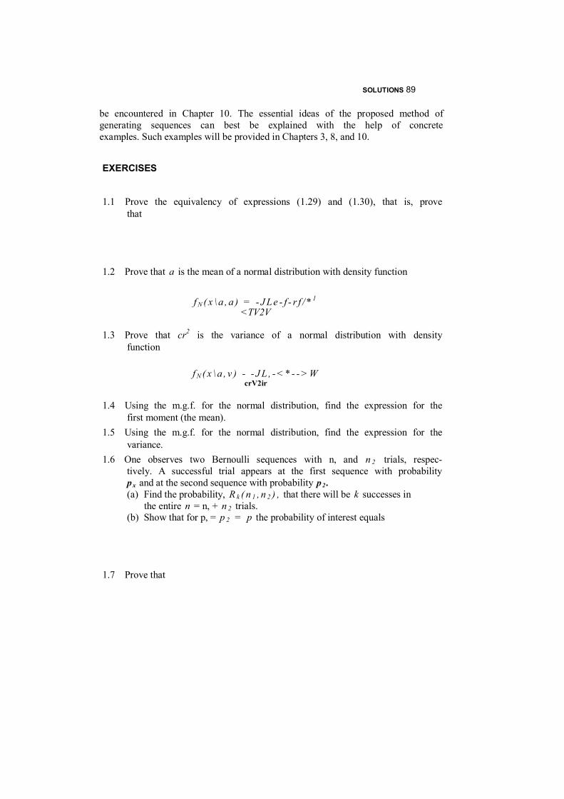
SOLUTIONS 89
be encountered in Chapter 10. The essential ideas of the proposed method of generating sequences can best be explained with the help of concrete examples. Such examples will be provided in Chapters 3, 8, and 10.
EXERCISES
1.1 Prove the equivalency of expressions (1.29) and (1.30), that is, prove that
1.2 Prove that a is the mean of a normal distribution with density function
f N ( x \ a , a ) = - J Le - f - r f / * 1 <TV2V
1.3 Prove that cr2 is the variance of a normal distribution with density function
f N ( x \ a , v ) - - J L , - < * - - > W crV2ir
1.4 Using the m.g.f. for the normal distribution, find the expression for the first moment (the mean).
1.5 Using the m.g.f. for the normal distribution, find the expression for the variance.
1.6 One observes two Bernoulli sequences with n, and n 2 trials, respec- tively. A successful trial appears at the first sequence with probability px and at the second sequence with probability p2 . (a) Find the probability, R k ( n 1 , n 2 ) , that there will be k successes in
the entire n = n, + n 2 trials. (b) Show that for p, = p 2 = p the probability of interest equals
1.7 Prove that
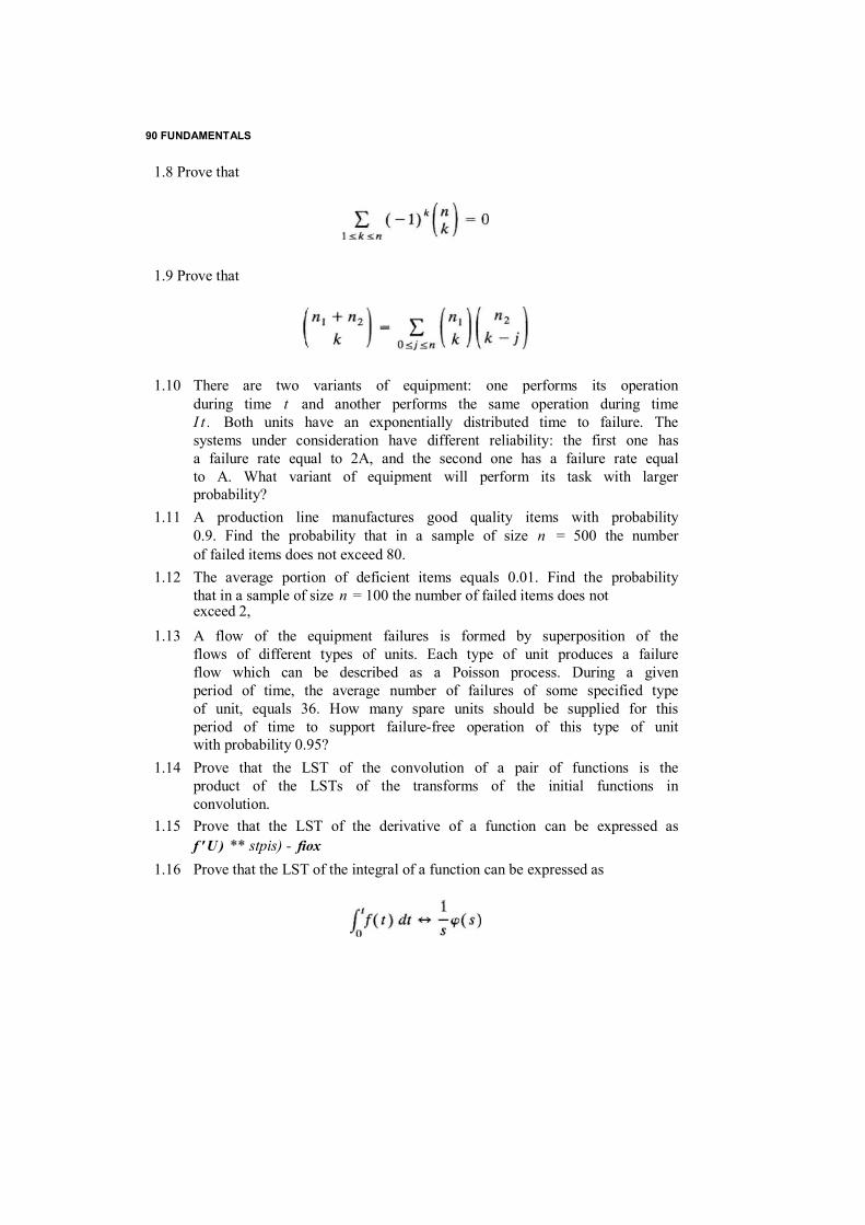
90 FUNDAMENTALS
1.8 Prove that
1.9 Prove that
1.10 There are two variants of equipment: one performs its operation during time t and another performs the same operation during time I t . Both units have an exponentially distributed time to failure. The systems under consideration have different reliability: the first one has a failure rate equal to 2A, and the second one has a failure rate equal to A. What variant of equipment will perform its task with larger probability?
1.11 A production line manufactures good quality items with probability 0.9. Find the probability that in a sample of size n = 500 the number of failed items does not exceed 80.
1.12 The average portion of deficient items equals 0.01. Find the probability that in a sample of size n = 100 the number of failed items does not exceed 2,
1.13 A flow of the equipment failures is formed by superposition of the flows of different types of units. Each type of unit produces a failure flow which can be described as a Poisson process. During a given period of time, the average number of failures of some specified type of unit, equals 36. How many spare units should be supplied for this period of time to support failure-free operation of this type of unit with probability 0.95?
1.14 Prove that the LST of the convolution of a pair of functions is the product of the LSTs of the transforms of the initial functions in convolution.
1.15 Prove that the LST of the derivative of a function can be expressed as f ' U ) ** stpis) - fiox
1.16 Prove that the LST of the integral of a function can be expressed as
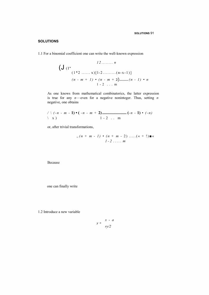
SOLUTIONS 91
SOLUTIONS
1.1 For a binomial coefficient one can write the well-known expression
1 2 . . . . . . . . n
(J ( I " ( 1 *2 . . . . . . x ) [ l - 2 . . . . . . . . . ( n - x - 1 ) ]
( n - m + 1 ) • ( n - m + 2) ........ ( n - 1 ) • n 1 - 2 . . . m
As one knows from mathematical combinatorics, the latter expression is true for any n —even for a negative noninteger. Thus, setting n negative, one obtains
/ \ ( - n - m - 1) • ( - n - m + 2) ........................ (- n - 1) • ( - n )
\ x ) 1 - 2 . . m
or, after trivial transformations,
„( n + m - 1 ) • ( n + m - 2 ) . . . . . ( « + ! ) ■ «
1 - 2 . . . . . m
Because
one can finally write
1.2 Introduce a new variable
x - a y =
ry/2
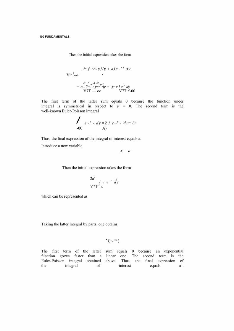
100 FUNDAMENTALS
Then the initial expression takes the form
~i= f ( o - y j l y + a ) e ~ y ' d y Vir J-a> '
n r _ 2 a _ 2 = o--7=- / ye y dy + -j=r I e y dy
V7T — oo V7T •'-00
The first term of the latter sum equals 0 because the function under integral is symmetrical in respect to y = 0. The second term is the well-known Euler-Poisson integral
e ~ y ~ d y = 2 I e ~ y ~ dy = /ir -00 A)
Thus, the final expression of the integral of interest equals a.
Introduce a new variable x - a
Then the initial expression takes the form
2a2 2 / y e y d y
V7T J-vi
which can be represented as
Taking the latter integral by parts, one obtains
+£•- ' '*)
The first term of the latter sum equals 0 because an exponential function grows faster than a linear one. The second term is the Euler-Poisson integral obtained above. Thus, the final expression of the integral of interest equals a1.
/

SOLUTIONS 83
L4 Consider (1.54). Assume that the first derivative with the substitution j = 0 derives the mean:
d I 1 2 A / j \ / 1 2
— exp^as + — a s j = (a + cr sjexp^as + ~<x s J
1.5 Using the intermediate
result of Exercise 1.4, one
obtains d d I = — ( a + <r2s) expl i ds y ' \
= a2 exp|«5 + + (« + ( r 2 s ) 2 exp|as + — cr2s2 j
= |cr2 + (as + a'2)2j exp|as + — <r3
This gives the second initial moment which is equal to the sum of the variance a2 and the mean squared a 2 . Substituting s = 0 gives the desired result.
1.6 Denote by b ( k , n ) the probability that there will be k successes in n trials. Then
(a)
and, finally,
(b) If p i ~ p 2 ^ p one can consider two experiments as one experi- ment with a total number of trials equal to n = « , + n 2 . For this case one has
p k q n ~ k
1.7 The solution follows immediately if one considers a binomial of the form (1 + 1)":
= a s - 0
d 2 d = d s
1 T as + —a 2s2
1
(HI .2)

84 FUNDAMENTALS
( i + i ) n = £ ( " W - 1 - £ ( " )
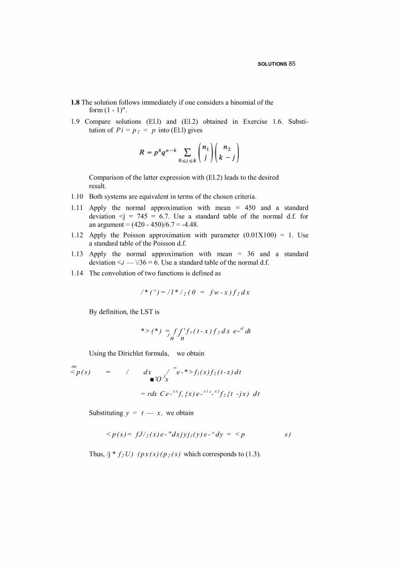
SOLUTIONS 85
1.8 The solution follows immediately if one considers a binomial of the form (1 - 1)".
1.9 Compare solutions (El.l) and (El.2) obtained in Exercise 1.6. Substi- tution of P i = p 2 = p into (El.l) gives
Comparison of the latter expression with (El.2) leads to the desired result.
1.10 Both systems are equivalent in terms of the chosen criteria. 1.11 Apply the normal approximation with mean = 450 and a standard
deviation <j = 745 = 6.7. Use a standard table of the normal d.f. for an argument = (420 - 450)/6.7 = -4.48.
1.12 Apply the Poisson approximation with parameter (0.01X100) = 1. Use a standard table of the Poisson d.f.
1.13 Apply the normal approximation with mean = 36 and a standard deviation <J — \/36 = 6. Use a standard table of the normal d.f.
1.14 The convolution of two functions is defined as
/ * ( ' ) = / l * / 2 ( 0 = f w - x ) f 2 d x
By definition, the LST is
* > ( * ) = f f ' f l ( t - x ) f 2 d x e~sl dt J n J n
Using the Dirichlet formula, we obtain
.oo < p ( s ) = / d x / e - * > f l ( x ) f 2 ( t - x ) d t
■'O Jx
= rdx C e - s x f , { x ) e - s i ' - x ) f 2 { t - j x ) d t
Substituting y = t — x , we obtain
< p ( s ) = f J / 2 ( x ) e - "d x j y j l ( y ) e - ^ dy = < p s )
Thus, /j * f 2 U ) ( p x ( s ) ( p 2 ( s ) which corresponds to (1.3).
.00
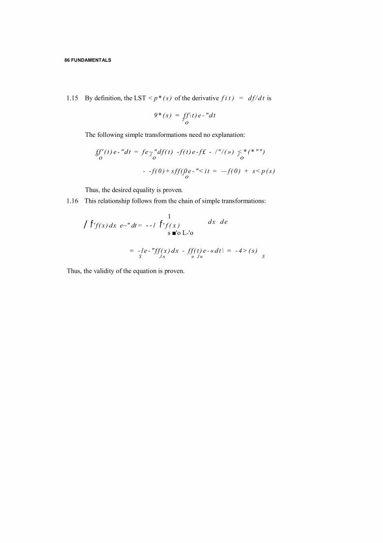
86 FUNDAMENTALS
1.15 By definition, the LST < p * ( s ) of the derivative f i t ) = d f / d t is
9 * ( s ) = f f \ t ) e - "d t J o
The following simple transformations need no explanation:
f f ' ( t ) e - "d t = f e ~ "d f ( t ) - f ( t ) e - f £ - / " / ( » ) < * ( * "" ) J o J o J o
- - f ( 0 ) + s f f ( 0 e - "< i t = — f ( 0 ) + s < p ( s ) J o
Thus, the desired equality is proven. 1.16 This relationship follows from the chain of simple transformations:
1
/ f' f ( x ) dx e~" dt = - - / f' f ( x ) s ■'o L-'o
= - l e - " f f ( x ) d x - f f ( t ) e - « d t \ = - 4 > ( s)
S J n n J n S
Thus, the validity of the equation is proven.
d x d e
CHAPTER 2
RELIABILITY INDEXES
Reliability indexes are basically needed for the quantitative characterization of a system's ability to perform its operations. These indexes must reflect the most essential operating properties of the system, be understandable from a physical viewpoint, be simple to calculate at the design stage, and be simple to check at the test and/or usage stage.
Sometimes it is practically impossible to characterize a system with only one reliability index. But, at the same time, the number of reliability indexes has to be as small as possible. Psychologists say that more than three numerical characterizations of the quality of some object can only lead to confusion and misinterpretation of a situation. Those who deal with multicri- teria optimization also know that the Pareto set should be of a small dimension. (One might recall the classical example from medieval French literature: the Buridan donkey died trying to solve a two-dimensional prob- lem when he could not choose one bunch of hay from two!)
Simultaneously, one has to avoid the use of different "integrated" or "weighted" indexes: Such indexes generally have no clear physical sense and may mask an unacceptable level of one index by uselessly high levels of the others.
Reliability indexes may not only be used for the characterization of a system as a whole, but also some of the indexes may have an intermediate character. For example, the system, considered as an independent object, might be characterized by an availability coefficient. If the same system is part of a more complex structure, it may be more reasonable to characterize it separately with the mean time to failure (MTTF) index and the mean repair time index because they might be used to more accurately express the complex system's availability index. Moreover, the system as a whole can be 86
Probabilistic Reliability Engineering. Boris Gnedenko and Igor Ushakov
1 00 RELIABILITY INDEXEScharacterized with indexes in the form of nondimcnsional real numbers. But for the system's subsystems, we sometimes need to know special functions (distribution functions, failure rates, etc.).
Almost all reliability indexes are of a statistical nature and depend on time. We now make several points about unrepairable and repairable (renewal)
units and systems. The distinction between repairable and unrepairable items is relative. The same system may be considered as repairable in one circum- stance and as unrepairable in another. The main indicator is a system's ability to continue its operation after repair. For example, a computer used for routine calculations with no special time restrictions may be considered as repairable. The same computer used for a noninterruptible technological process or in a military action (which is almost always dangerous if inter- rupted!) may be considered as unrepairable. But if in the latter case the computer is used in an on-duty regime, it might be considered as repairable during the idle period.
Of course, some technical objects are essentially unrepairable. Some of them, such as a light bulb, cannot be repaired at all. As another example, a missile cannot be repaired during its mission. For convenience, in these cases we speak of a "renewal socket" in which unrepairable units are installed one after another in the case of a failure. Thus, after a first unsuccessfully launched missile, another one may be launched; after a first bulb has failed, another one may replace it.
2.1 UNREPAIRABLE SYSTEMS
2.1.1 Mean Time to Failure If the criterion of a system's failure is chosen and perfectly well defined, we can determine its reliability indexes, in particular, the mean time to failure (MTTF).
After observing N failures of N unrepairable systems, there are records of nonnegative values: t ,, t z , . . . , t N . One of the most natural characteristics of this set of observations is the sample mean, or the mean time to failure (MTTF):
r - ( i / AO ( f , + r 2 + • • • +'N) (2-1)
This reliability index means that the system, on average, works T time units before a failure.
Consider these values in increasing order, that is, present the observations as
t \ < < 2 < ■ ■ ■ <
UNREPAIRABLE SYSTEMS 89 In this new notation the following equivalent equation can be written:
T = N t \ + ( N — 1 ) ( t ' 2 - * ' , ) + • • ■ +(t'N - t'^)
The equivalency of the formulas follows from consideration of Figure 2.1 where a histogram of the values t k is presented. If a prior distribution F i t ) of a system's TTF is known, the expected value of T can be calculated in the standard way:
(2.2)
For nonnegative random variables, the following equivalent expression can be written (see Exercise 2.1)
(2.3)
where P i t ) = 1 - F i t ) . The equivalency of (2.2) and (2.3) follows from the fact that we are only using different means of integrating the same function (see Figure 2.1). On a heuristic level this result may be explained by comparing this case with the analogous discrete case depicted by Figure 2.1. The reliability index MTTF is very convenient if the system's outcome linearly depends on the time of its successful performance. For example, consider a form for producing some plastic item. After a failure the form is replaced by a new one. Thus, this form can be considered as a socket in the above-mentioned sense. In this case the effectiveness of using the form depends only on the average time to failure. But in other cases this reliability index may prove to be inconvenient.
2.1.2 Probability of a Failure-Free Operation Consider a system performing an operation with a fixed duration tQ. In this case each t k < t 0 corresponds to a system failure. A natural reliability index in this case is the probability of a failure-free operation, which reflects the frequency of appearance of the condition tk > tQ. We introduce the so-called indicator function
otherwise
In other words, we define a system failure in a new form: the system fails when d = 0.
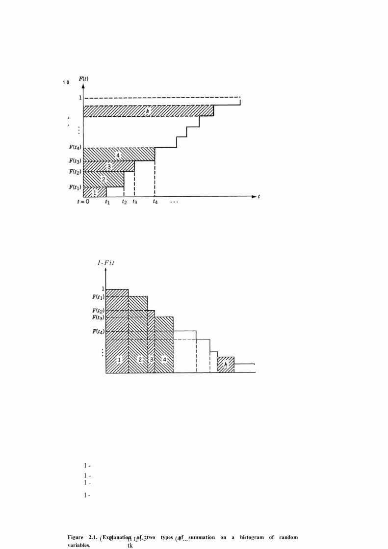
1 00 RELIABILITY INDEXES
FUk)
I - F i t)
1 -1 -1 -
1 -
( = 0 (i t2 t-3 (4 ... tk
Figure 2.1. Explanation of two types of summation on a histogram of randomvariables.

UNREPAIRABLE SYSTEMS 91 For the same data we have to calculate the new reliability index as
P( t 0 ) = ( l / N ) ( d i + d 2 + ■ ■ ■ + d N )
where d k = d ( t k , f()). If we know the distribution F i t ) of the system TTF, the probability of a successful operation can be expressed as
P{ l 0 ) = 1 - F ( t 0 )
Sometimes the duration of a task is a random variable itself, with a distribution H i t ) . We may then speak about the expected probability of success for the random performance time. The general expression for this index is
/ > = f p { t ) d H { t ) (2.4) J o
Several particular cases are considered in Exercise 2.2.
2.1.3 Failure Rate As we mentioned above, we sometimes have to know some special functions in order to calculate the reliability indexes of a complex system. One such important function is the failure rate A(f). In strict probabilistic terms this is the instant conditional density function at moment t under the condition that the random variable under consideration is not less than t , that is,
/CO AC ) - J^ (2.5)
At first this function, called the hazard rate, appeared in demography connected to the insurance business. The physical sense of this function can be easily explained in the following simple terms. If we know the prior distribution F i t ) with density /(/), then an element of the conditional probability
Pr( d t \ t ) = A(0 d t
is the probability of the death of an individual of age t during the forthcom- ing time interval [/, / + d t ] . This function has exactly the same sense in reliability theory when one substitutes the corresponding terms. We refer to this function as the failure rate. To explain it, consider the uniform distribution F i t ) on the interval [0,10]. In this case A(0) = /(0) = 0.10 because P(0) = 1 for a nonnegative r.v. Next, consider the moment t = 1. The area of the domain for the r.v. under
1 00 RELIABILITY INDEXESthe condition that it is larger than 1 become smaller: now it is [1, 10]. So A(l) = 1/9. Of course, the same result can be obtained directly from (2.5) if we substitute /(l) = 0.10 and P(l) = 0.90. Then for the next moment, say t = 5, we have A(f) = 0.20; for t = 9 we have AO) = 1.0; for t = 9.9 we have A0) - 10.0; for t = 9.99 we have AO) = 100.0; and so on. The function AO) approaches o° at ( = 10.
For a norma! distribution with mean a = 10 and standard deviation a = 1, we can calculate AO) using a standard table of the normal distribution.
In both cases we observe that the function AO) is increasing and un- bounded. Thus, the unit's reliability for such a TTF distribution becomes worse in time. Such an aging process is very natural for most real objects. But this type of increasing function is not the only one. As we considered in Chapter 1 for the exponential distribution, the failure rate is constant in time. Moreover, the so-called "mixture of exponential distributions" has a monotonically decreasing function AO).
For the mixture of two exponential functions, we can write
F ( t ) = 1 -p[exp(-avf)] - (1 — p ) [exp( ~ a 2 t )] (2.6)
The expression for A(r) can easily be obtained
_ ^ a i [ e x P( _ a i O ] + 0 ~P)«i|"PC-«2*)l p[exp(-a,0] + (1 -p)[exp(-a2/)]
We will analyze this equation "on a verbal level" using only simple explanations. For f = 0 we have
A(0) -pa, + (1 - p ) a 2
that is, A(0) is a weighted hazard rate at this moment. Then note that the function AO) is a monotonically decreasing function. If a, > a2, then lim, AO) = a2. From (2.5) it follows that
This immediately yields
- f ' \ ( x ) d x J i i
d P (t ) d t n o
d F{ t ) d t
P ( t )
d[InP(0] A(r) = d t
P ( t ) = exp (2.7)

UNREPAIRABLE SYSTEMS 93 From the condition 0 < P ( t ) < . 1, it follows that, for any t ,
0 <; [ ' \ { t ) d t < oo J o
and
lim f ' x ( t ) dt -* oo
Thus, the function is such that A(f) > 0 and possesses properties (2.7) and (2.8). In most practical cases we observe a so-called "U-shaped form" of the function A(r), as depicted in Figure 2.2. During the first period of time, we observe a "burning-out" process. This process consists in the early failing of weak or defective items. Then follows a period of "normal" operation during which the failure rate is constant. During this period a failure only occurs "completely incidentally," or, as one sometimes says, "as a brick fallen from the roof." It is a period of wcaring-out, fatigue, and other normal phenomena of aging. We will show below that qualitative knowledge about the failure rate is very important for reliability analysis.
2.2 REPAIRABLE SYSTEM
2.2.1 Description of the Process During the observation of a repairable system, we can record the sequence of periods, each of which consists of a successful performance time plus an idle
m
Figure 2.2. U-shaped function of A(f).
1 00 RELIABILITY INDEXES
time. Such a process is illustrated in Figure 2.3. Let denote the random time from the completion of the (k - l)th repair to the k th failure, and jet 7jk denote the duration of the fcth repair (renewal).
In the simplest case with a socket (a one-unit system), we suppose that a repair is equivalent to the replacing of a failed unit. This corresponds to a complete renewal. In this case we consider an alternating stochastic process with i.i.d. r.v.'s £ and 17, having distributions F i t ) and G i t ) , respectively. We denote this alternating stochastic process by 7 7 } .
Of course, the corresponding process for a system consisting of several renewal units may be much more complicated. Almost all the following explanations will be—for simplicity—presented for a renewal unit, or a socket.
All indexes used for an unrepairable system can also be used in this case for the appropriate purpose. But for repairable units and systems wc have to consider several special indexes. They are more complicated and need more explanation.
2.2.2 Availability Coefficient Consider a system which has to work in a "waiting" regime and, at the same time, the duration of the task performance is negligibly small. In this case a natural reliability index is the so-called availability coefficient K i t ) , This index is the probability that the system will be in an operating state at a specified moment ( in the future.
The numerical value of K i t ) depends on the specified moment of time t . For example, if we know that at t — 0 the system is new and, consequently, is in an operating state, then at moment e , where e is small, the probability that the system is in an operating state is close to 1 and approximately equals K i e ) = Pie).
The behavior of K i t ) in time can be periodically attenuating or strictly attenuating. This depends on the types of d.f,'s F i t ) and G i t ) . For illustra- tive purposes, consider the case where Fit) is a normal d.f. with a small coefficient of variation k and G i t ) is a degenerate function (i.e., 17 is constant). K i t ) for this case is presented in Figure 2.4.
It is clear that the first time to failure has a normal d.f. with some mean T and a relatively small <7. The renewal completion time has the same distribu- tion biased on the time axis. If r\ > 3a-, there may be some interval between T and T + 7 7 where K i t ) = 0. The second time to failure also has a normal
Figure 2.3. Graphic description of an alternating process.
UNREPAIRABLE SYSTEMS 95
--------------------------------------------------------- Figure 2.4. Example of the oscillating behavior of Kit) in time.
d.f. but with the standard deviation larger by times. Thus, the zone between 2T and 2(T + TJ), where K i t ) = 0, will be smaller. Finally, for ( » T + 7j, K i t ) will be almost constant. If both d.f.'s F i t ) and G i t ) are exponential, the function K i t ) is strictly decreasing with exponential speed. We will consider this case later. For large t the initial state has practically no influence on the behavior of K ( t ) . In this case the probability that the system is in an operating state equals the proportion of the total up time to the total operating time. Later we will show that for this case
E U ) K = —' - (2.10)
The index K is called the stationary availability coefficient, or simply, the availability coefficient. Sometimes we are interested not in a "point" characteristic K i t ) but in the average time spent in an operating state during some period of time, say t . We introduce the index
1 f t K * ( t ) = - / K { x ) dx
t J Q
If t - * oo, both K i t ) and K * i t ) have the same limit, namely, K defined in (2.10).
2.2.3 Coefficient of Interval Availability If the duration of the system's task is not negligibly small, we speak about the coefficient of interval availability, that is, the probability that at a time t the
Kit)

1 00 RELIABILITY INDEXESsystem is found in an up state and will not fait during the performance of a task of length, say tn. Denote this index R i t , r„):
i?(M0)=X(r)/»(/0ir)
We will consider this index later in more detail but now we note that P(r0[r) = P( t { ) ) only when F i t ) is exponential.
If the system is not a socket with renewal unit, the situation is more complicated. In Chapter 7 we will illustrate this statement on a duplicated system consisting of two identical renewal units.
2.2.4 Mean Time Between Failures and Related Indexes Mean Time Between Neighboring Failures In general, the mean time to a first failure 7(]) differs from the mean time from the first repair termination to the second failure T(1), and so on. In other words, all intervals of failure-free operations T ( k ) , k = 1 , 2 , . . , , may be different. We consider several typical situations.
For a socket, or a one-unit system, the MTBF coincides with the MTTF because a new unit, put into the sockct, is supposed to be identical to the failed one. But this equivalence of the MTTF and MTBF cannot be ex- tended, even for the simplest two-unit system.
Consider a Markov model of a redundant system of independent and identical units [in other words, both F ( t ) and G i t ) are exponential]. Assume that we know how to compute the mean time to a forthcoming failure for this system for the following two cases: starting with the state when two units arc up (T12'), and starting with the state when only one unit is up (T1®1) (see Figure 2.5).
On average, the time to failure from state 2 is larger than the TTF from state 1. Indeed, in order to fail starting from state 2, the system must first enter slate 1 and then from this state transit to the failure state. (Of course, from state 1 the system might even return to state 2 again.) In other words, jlA = j* + where T* is the time of the system staying in state 2 until entering state 1.
In this particular case all of the remaining intervals of failure-free periods are i.i.d. r.v.'s, because for this particular Markov process all of the initial conditions are the same.
Now consider the behavior of a series system of two independent units. For simplicity, suppose that the repair time is negligible. Let each unit have a normal d.f. of TTFs with a mean T and a very small variation coefficient. If at the moment t = 0 both units are new, then the first and second failures of the system are expcctcd to appear close to cach other and are around t = T . If the random TTFs of the units are denoted by £, and £2, respectively, then r[(] = min{£j, £2) and T [ 2 ] = max{£„ £2) - min{£„ If the r.v.'s f s are as

UNREPAIRABLE SYSTEMS 97 - - e ? — % 2 M - - - - e3-
(a)
c e2 >■ %2
( b )
Figure 2.5. Examples of two time diagrams for a two-unit system: (a) a system of independent units; (£>) a system working until both units have failed.
described, = E{£}, and T [ 2 ] has the order of <r. By assumption, A- T (see Figure 2.6). The next couple of failures are expected to appear close to t = 2 T , but the expected deviation is J2 times larger than the initial deviation. For the case A « T,
rpi- + + (2.11)
and
r(4] = max(^> + ^>,^) + ^>) (2.12)
[Notice that strictly speaking (2.11) and (2.12) should be expressed in a more complicated way. We must take into account the mixture of the failure flows of the two sockets. This is explained by the appearance of extremely small and extremely large r.v.'s.] Thus, if 7[|) > T [ 2 ] , then T [ 2 ] < 7*[3] and r[4] < r[3j. At the same time, 7"(l] > 7p, and r[2] < 7"[4j. The process continues in the same manner for larger numbers of intcrfailure intervals.
T{ \ ) T ( 2 ) T( 3) T{4) T { 5) T(6)
-x ---------- o—x --------------------- x o x -------------------------------x o x ---------------------------- t T 2 T 3 T
Figure 2.6. Example of the failure flows of a series system of two units.
i 1 n

UNREPAIRABLE SYSTEMS 98 With rt s> 1, for any variance a2, the value ajn begins to be larger than T . This leads to a strong mixture of moments of failure of both sockets of the system. In theoretical and practical terms, this means that Tj^j ~ + and, moreover, T[n] -> » with n -» «>. Thus, even for the simplest two-unit system, all MTBFs are different (though they may have the same asymptotical value). More complex cases appear when we consider a series system of more than two units. Notice that in reliability theory the term MTBF is usually used for the stationary regime, that is, as t - *
There are other indexes used in reliability theory which are connected with the time to failure. One of them is the instantaneous MTTF at time t . This is the mean time to failure from a specified moment t under the condition that a failure has happened just at this moment. From qualitative arguments it is clear that for t comparable with T this new index will differ from the MTTF. We remark that for the stationary regime, the values of both of these indexes coincide.
To conclude the discussion about the MTBF, we must emphasize that each time one should understand what kind of a particular TTF is under consider- ation. If we again regard a renewal series system of n units, each of them with a normally distributed TTF with a very small coefficient of variation, then we have the following:
1. For the MTTF
T ~ min 1 £/s;n
2. The next n — 1 MTTFs might be extremely small depending on the number of units and the smallness of the variation coefficient:
j(I) _ E{£1 '+ I) -
where is the i'th-ordered statistic, 1 < i < n - 1. A possible behav- ior of t ( k ) for a series system is presented in Figure 2.7.
3. The stationary MTTF for any recurrent point process with continuous distributions of TTFs is
7 =
T 1 &i<.n i
This value is the limit for T { k ) when k - » oo.
In practice, we are often interested in the mean time of a failure-free operation starting from some specified moment t . In the theory of renewal

SPECIAL INDEXES 99
I ------1 ----- 1 ----- 1 ----- 1 ----- 1 ----- 1 ----- 1 ----- 1 ----- 1----- 1 --- J<0) -jil) j(2) J(3) jii] fi 5) J<6] y(7) y<8> j«9) jilO)
Figure 2.7. Example of changing the mean time between failures depending on the current number of failure for which this value is evaluated.
processes, this value is called the mean residual time. In general, this index differs from the MTTF and any version of the MTBF.
If t -» oo, for a recurrent process this index differs from both of those mentioned above. The exception is a Poisson process for which all three indexes coincide.
2.3 SPECIAL INDEXES
Now we consider some special reliability indexes for repairable systems. These indexes are nontraditional: they describe not a failure-free operation but rather a successful operation during a specified time. In some sense, there is no "local" failure criterion. The determination of a succcssful or unsuccessful operation is made, not at the moment of a current failure, but only after the completion of the entire system's performance during an acceptable operational time. This means that some interruptions of the system operation might be considered as not being destructive.
2.3.1 Extra Time Resource for Performance Sometimes a system has some reserve time to perform its task; that is, the interval of time 60 given for the performance of the system operation is more than the time t 0 required for a successful operation.
Examples of such situations can be taken from different areas of applica- tions: conveyer production lines, electronic equipment with special power supplies, a computer performing routine calculations not in real time, and so forth. (Other detailed examples will be provided below.) In all of these cases not all failures of the system lead to the failure of the overall system's performance.
Consider a computer performing a computational task whose duration is f0. The computer has a resource of time 9 0 for its performance which is
1 00 RELIABILITY INDEXESlarger than the required time t0. Random negligibly short interruptions (errors) may appear, each of which will destroy the results of all of the performed calculations. In this case the probability of success can be written as
Pr{at least one t k > t ( ) \ k : t k e 0O}
Let the computer's task be segmented into phases and assume that the computer works in a restarting regime. After the completion of each phase, all intermediate results are put into the computer's memory. Each short failure has destroyed only the very last phase of the overall solving task. After the error has been found, the calculations for this particular phase are repeated. We do not give the formal definition of the corresponding reliabil- ity index but it is understandable that this index may be defined with the help of (2.13). We will consider this case in the special section dedicated to time redundancy.
2.3.2 Collecting Total Failure-Free Time Suppose a system is required to accumulate some given amount of successful operating time during some given period 9 0 for the successful performance of the task. The probability of success can be written as
(2.14)
As an example, we may again consider a computer system with a restarting regime for which each failure takes some time to repair but the operation of the system can be continued without loss of the previously obtained results. This situation may be observed if the restarting phases are very short, so there is practically no loss of the intermediate results but the system needs some time for restoration.
A close phenomenon occurs when one considers the transportation of some load. Failures and consequent repairs may only delay the termination of the task, but will not lead to a total failure. Of course, if the total idle time exceeds some limit, the task should be considered as not fulfilled (e.g., in the transportation of fresh food).
This index can obviously be written as
(2.15)
where is the specified allowable total down time during the period 0O.
k
(2.13)
k


1 00 RELIABILITY INDEXES2.3.3 Acceptable Idle Intervals Some systems possess the property of time inertia: they are insensitive to short breakdowns. As an example, consider a responsible computer system which has an independent power supply to prevent the system from occa- sional short failures of the common power system. In this case, if a failure of the main power system occurs, the computer system can operate with the help of this spccial power supply. Another example can be represented by a multistage conveyer system with an intermediate storage of spare subprod- ucts in the case of a breakdown in the previous stages.
Thus, roughly speaking, an operational interruption of any such system can be noticed only if the duration of the down time x k exceeds some specified value jc0. In this case the reliability index is
Prfall x k < JE,,!.** e fl0} (2.16)
In real life wc meet more complicated situations. For example, a redundant power supply may demand substantial time to recharge, and this fact must be taken into account.
Of course, some combinations of the listed criteria for a system's failure may be considered. Some of them will be presented later.
2.4 CHOICE OF INDEXES AND THEIR QUANTITATIVE NORM
2.4.1 Choice of Indexes The problem of choosing a reliability index arises before an operations research analysis. The solution of this problem depends on the nature of the object to be analyzed, its operations, and its expected results.
Depending on the operational level of the system, reliability indexes can be divided into two groups: operational and technical. If we deal with a system performing its individual and independent operation with a concrete final output, the reliability indexes should characterize the system's ability to perform its operation successfully. Such indexes are called operational.
If we deal with an object that is a subsystem and only performs some functions that are necessary to fulfill the operation of the system as a whole, the reliability indexes may be auxiliary. We can express the operational indexes of the system as a whole through these indexes. Such indexes are called technical. They are used to describe the reliability of a system's components and parts.
Starting with operational indexes, consider a computer that can be used to perform several quite different operations. The computer which is used for routine calculating tasks may be characterized with the help of an average percentage of useful operational time. The availability coefficient is the appropriate reliability index in this case.

CHOICE OF INDEXES AND THEIR QUANTITATIVE NORM 101
The same computer used for supporting a long and noninterrupted techno- logical process can naturally be characterized by the probability of a failure- free operation (PFFO).
If the computer is used for an automated landing system in an airport, and the duration of each operation is negligibly small in comparison with the computer's mean time to failure (MTTF), the reliability index should reflect the number of successfully served airplanes. In this case the availability coefficient is also the most appropriate reliability index.
If the same computer is unrepairable, for instance, its task consists of collecting and processing information in a spy satellite, the best characteriza- tion of it is the MTTF.
In all of these cases the reliability index corresponds to the system predestination and to the nature of its use.
Now consider an example when a reliability index is used to characterize "inner" technical abilities. Consider two identical computers connected in parallel. The natural reliability index for this duplicated system is the PFFO. In this case each computer is only a subsystem taking part in the performance of a system's operation. What should we know about each separate computer to characterize this system? To compute the complex PFFO, one needs to know the probability distributions of both the time to failure and the repair time of the computer, as well as the parameters of these distributions. The distribution itself is not an index; it is a function. But parameters of the distribution can be considered as technical reliability indexes of the com- puter. These parameters have no relation to a system's operation, they only reflect an ability to work in general.
Note that the type of reliability index chosen does not depend on the responsibility of the performed operation. The responsibility of the system's operation defines the level of requirements but is not part of the nomencla- ture of reliability indexes.
When choosing reliability indexes we should take into account the follow- ing simple recommendations based on common sense:
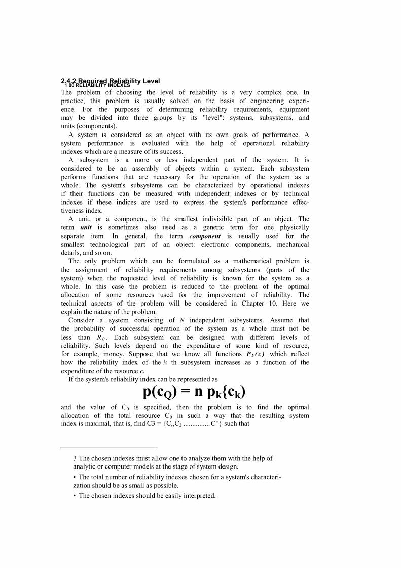
1 00 RELIABILITY INDEXES2.4.2 Required Reliability Level The problem of choosing the level of reliability is a very complcx one. In practice, this problem is usually solved on the basis of engineering experi- ence. For the purposes of determining reliability requirements, equipment may be divided into three groups by its "level": systems, subsystems, and units (components).
A system is considered as an object with its own goals of performance. A system performance is evaluated with the help of operational reliability indexes which are a measure of its success.
A subsystem is a more or less independent part of the system. It is considered to be an assembly of objects within a system. Each subsystem performs functions that are necessary for the operation of the system as a whole. The system's subsystems can be characterized by operational indexes if their functions can be measured with independent indexes or by technical indexes if these indices are used to express the system's performance effec- tiveness index.
A unit, or a component, is the smallest indivisible part of an object. The term unit is sometimes also used as a generic term for one physically separate item. In general, the term component is usually used for the smallest technological part of an object: electronic components, mechanical details, and so on.
The only problem which can be formulated as a mathematical problem is the assignment of reliability requirements among subsystems (parts of the system) when the requested level of reliability is known for the system as a whole. In this case the problem is reduced to the problem of the optimal allocation of some resources used for the improvement of reliability. The technical aspects of the problem will be considered in Chapter 10. Here we explain the nature of the problem.
Consider a system consisting of N independent subsystems. Assume that the probability of successful operation of the system as a whole must not be less than R 0 . Each subsystem can be designed with different levels of reliability. Such levels depend on the expenditure of some kind of resource, for example, money. Suppose that we know all functions P k ( c ) which reflect how the reliability index of the Ac th subsystem increases as a function of the expenditure of the resource c.
If the system's reliability index can be represented as
p(cQ) = n pk{ck) and the value of C0 is specified, then the problem is to find the optimal allocation of the total resource C0 in such a way that the resulting system index is maximal, that is, find C3 = {C,,C2 ............... C^} such that
3 The chosen indexes must allow one to analyze them with the help of analytic or computer models at the stage of system design. • The total number of reliability indexes chosen for a system's characteri- zation should be as small as possible. • The chosen indexes should be easily interpreted.
CHOICE OF INDEXES AND THEIR QUANTITATIVE NORM 103
P(C*) = maxf n P k { C k ) E Q < C 0 \ I 1 l z k & N I
• The indexes should allow one to formulate clear requirements on relia- bility. • The indexes must allow one to estimate the achieved reliability level after field tests or experimental exploitation. • Complex "integrated" indexes must be avoided: various "convolutions" and "weightings" of different indexes usually have no real meaning.
1 00 RELIABILITY INDEXESOf course, we might also formulate the inverse problem: to design a system with a required level of reliability, for example, R0. Then the problem may be reformulated as
A solution to both of these problems is presented in Chapter 10.
Unfortunately, even such simple problems cannot usually be solved in practice because the functions P k ( C k ) are often unknown. In such cases we usually use heuristic methods based on a proportional distribution of reliabil- ity "quotas" among the system's units.
What must one do in the general case when it is necessary to assign a reliability level to the system as a whole? In our opinion, there is only one thing to do: perform an evaluation based on engineering experience. Proto- types can be used for comparison with the designed system and, on the basis of this, the decision about a possible or desirable reliability level might be made.
Naturally, if one fixes the amount of available resources for the production of some type of technical system, then we not only have to solve the problem of an optimal reliability level, but we must also answer the question of how many such systems we intend to produce? In turn, the number of systems of some chosen type depends on the number of other "competing" systems in the same area of use or utility. Assume that we are considering the design of a new type of jet. First of all, too high a level of reliability wiii demand a high level of expenses for the production of each jet and, as a consequence, will lead to a decrease in the total number of jets produced. It is clear that it is useless to have only one extremely highly reliable jet and it is equally unreasonable to have a large number of jets, each of which has a very low reliability. To choose "a golden middle" is a problem which lies outside the scope of mathematics and even outside the scope of engineering. The only way to solve this problem is to rely on expert's opinions and traditions.
But the experts' opinions are also not isolated. Taking into account all considerations concerning this particular type of a jet, experts have to think about the number and reliability of other jets owned by the airline. But this total number depends on a specific situation, considering the transportation system of the country as a whole. In turn, it depends on the level of the national economy. The level of the national economy depends on a number of unformulated and nonformulated factors: the political stability of the country, the external situation in the world, and so forth. Thus, we are convinced that any attempt to try to solve this problem in some "precise" sense is doomed.
But then one may ask: Why use mathematical methods at all? Why not rely on experts' opinions to solve all problems of this kind? The answer is that
P(C*) = min Pk(Ck)zR
CHOICE OF INDEXES AND THEIR QUANTITATIVE NORM 105
mathematical methods of analysis of situations help one to make logically strong decisions; mathematical models of technical systems help one to understand the nature of systems being designed. We begin to make local solutions in optimal ways. This leads to a kind of process of "natural selection." As in nature this process allows for the survival of only those who have best adapted to existing environments. And, in this situation, those technical systems which are "locally optimally designed" have a better chance to "survive" under currently existing circumstances.
We now consider possible methods of establishing reliability.
System Level Consider two principal cases. One of them consists in the use of practical experience and engineering intuition. Mostly it is based on an analysis of prototypes of the new technical system to be investigated. This method needs no special comments.
Practically, the only time a system's reliability requirement appears is if:
- The system's outcome can be measured in cost units, that is, in the same units as the costs of the system's design, production, and maintenance.
• The system's structure and operational modes are well known in ad- vance.
• Necessary statistical data for all components are determined with a satisfactory degree of confidence.
In this case the designer has an opportunity to compare M different variants of the system's design and to choose the most profitable one. The objective function of the system's performance for the fcth variant can be written in the form
F k ( R ) = E k ( R ) - y C k ( R)
where R is the system's reliability index, E k ( R ) is the outcome of the &th variant of the designed system, and C k ( R ) is the expenditure needed to design, produce, and maintain the system with index R , \ < k < M and -y is a dimensional coefficient analogous to a Lagrange multiplier. The value of R depends on the structure of the fcth variant, S k , and on the reliability indexes of the subsystems used, r j k \ \ < i < n k , where n k is the number of subsys- tems in the £th variant of the system. Thus, R itself can be written in a general form as
R = R ( S k , r } k H \ < k < , M , \ < n k )
For simplicity, suppose that all functions are differentiate. Then the optimal level of the reliability index R can usually be determined by solving the equation
d
1 00 RELIABILITY INDEXES
or, equivalently,
d E k ( R ) d C k { R) d R d R
Each optimum can be evaluated and then the variant k with the highest value of F k ( R k
p t ) is selected. Unfortunately, such an ideal situation appears extremely rare in engineering practice.
Subsystem Level Suppose that the system's reliability requirement is specified. Then the problem is to distribute the given value of the index over the subsystems. We consider several cases, each of them representing differ- ent information concerning the system's structure and the availability of statistical input data.
Uniform Allocation of Requirements This method is usually used when one can imagine only the approximate size of a subsystem of the main system. A reliability index R of a probabilistic nature (e.g., the probability of success or the availability coefficient) is specified for the system as a whole. The simplest assumption is that the system has a series structure and consist of n subsystems. The reliability requirement for each subsystem is then given by
R ^ TR I < i < n
Clearly, if subsystem indices are chosen in such a way, the system reliability index equals R . If requirements can be specified as the system's MTTF T , we can choose for each ith subsystem
r , = n T
This means that we additionally assume that the TIT of any subsystem has an exponential distribution.
Allocation in Proportion to the Number of Units Assume that the same conditions exist as before, but in addition subsystem / consists of «, units which are essentially similar in their complexity. In this case the requirement (in terms of the probability of success) should be chosen to be
Rt = "IfR 1 z i < n (2.17)
where
n , ai = —= -------
L n i I z i s N

1 00 RELIABILITY INDEXES
This method can be useful if different subsystems are designed by different subcontractors. It is reasonable to specify "softer" demands for more com- plex subsystems.
Allocation in Proportion to the Expected Failure Rate Suppose a de- signer has more complete information about the system: the unit failure rates are known (perhaps from previous experience), and the hypothesis about the exponential distribution can be considered valid. In this case the previous method can be improved. We can use (2.17) but we substitute at defined by
£ A jfiji _ ) z j s M _____________
£ £ V/i lsisn 1 S j < M
where M is the number of types of units and n« is the number of units of the yth type in subsystem i.
Optimal Allocation of Reliability Requirements This method is applied if we know the system's structure 5 and can predict the cost-reliability trade-off for each subsystem. The problem is to find the values of 1 < r < n , that yield the required reliability index at the lowest cost. This problem can be written in mathematical terms as
rainj £ C, (K,) | j l (* , , l*f s i» |S);fc*o} \ I £i' I
where C^R,) represents the subsystem's costs as a function of its reliability and 5 is the conditional notation of the system structure. For instance, if we consider a series system, the reliability function can be represented as
KWCiMsfsfia) - n Ri(C() 1 S i S n
In other words, the optimal allocation of reliability requirements between subsystems is a type of optimal redundancy problem (see Chapter 10).
T
When all distributions are assumed to be exponential, the requirementscan be formulated in terms of the MTTF as

EXERCISES 107
Reliability Requirements for a Component Almost all equipment com- ponents in engineering are of general usage. The only method in this case is based on the "natural selection" principle. In other words, the better and cheaper components among existing ones survive the competition in a techni- cal and economic environment. And, at the same time, new components appear and replace technical "dinosaurs."
CONCLUSION
This chapter does not need any special comments. In one form or another, reliability parameters are discussed in any book on reliability engineering or theory. As examples, we refer the reader to the wide list of general refer- ences at the end of this book.
The nomenclature of reliability indexes in a systematic and structured form can be found in Kozlov and Ushakov (1970) and Ushakov (1985, 1994). The methodological problems of choosing indexes and quantitative requirements in reliability engineering are discussed in Gnedenko, Kozlov, and Ushakov (1969).
REFERENCES
Gnedenko, B. V., B. A. Kozlov, and I. A. Ushakov (1969). The role and place of reliability theory in engineering. In Theory of Reliability and Queuing Systems (in Russian). Moscow: Nauka. Kozlov, B. A., and I. A. Ushakov (1970). Reliability Handbook. New York: Holt,
Rinehart, and Winston. Kozlov, B. A., and I. A. Ushakov (1975). Handbook on Reliability of Radio and
Automation Systems (in Russian). Moscow: Soviet Radio. Ushakov, I. A., ed. (1985). Reliability of Technical Systems: Handbook (in Russian).
Moscow: Radio i Sviaz. Ushakov, I. A., ed. (1994). Handbook of Reliability Engineering. New York: Wiley.
EXERCISES
2.1 Prove that the mean value of a nonnegative r.v. v with distribution Fit) can be expressed in the form of (2.4) which is equivalent to (2.3).
2.2 A system has an exponentially distributed TTF with parameter A. The operation to be performed also has a random duration. Find the

1 00 RELIABILITY INDEXES
probability that the system successfully performs its operation if (a) the operation duration is distributed exponentially with parameter
a; (b) the operation duration is distributed normally
fN(x \a, <r) = ayzir
with mean equal to a and variance equal to a2 . We also assume that ACT 1.
2.3 Build the graph of the failure rate for the mixture of two exponential distributions (2.6) with the following parameters, respectively,
(a) A, « 1 [1/hour], A2 « 1 [1/hour]; (b) A, = 0.5 11/hour], \2 " 1 [1/hour]; (c) A, = 2 [1/hour], Aa = 1 [1/hour],
SOLUTIONS
1.1
r = f t d F ( t ) = f t d [ I - / > ( * ) ] = - f t d p ( t )
'o •'o
and, after integrating by parts,
- f tdPit) = - tP(t) + fV(f) d t = r^ iO d t = A1 ~ ^0)3 dt
1.2 (a) Using (2.4), one writes
/>= re-Xxae-~*dx - aCe'^^dx =» -'O ■'O A + A
(b) First of all, consider the given conditions. Almost all "probabilistic mass" is concentrated in a relatively very compact area related to the MTTF of the system. This means that in this area the exponen- tial function can be successfully approximated by the set with at most two terms:
(A*) 1 - Ax +
SOLUTIONS 109Thus, one has
/>= r e-X x fN(x \a,<r)dx = r
(A xy f i f C Vn A i = / fN(x \a,a)dx - I x\a,cr) dx + / —-—fN(x \a,a)dx
'n •'n J n A (a\y
= 1 - aX +
In the first case there is no mixture at all; the second and third cases differ only by the scale. In general, one can write
/ (f) =p,A ] e- A" + p2k 2e~^'
p , k . e + p2 \2e
A(/)
pxe *«' + p2e
(The numerical solution is left to the reader.)
(A XY fN(x \a,tr)dx 1 - Ajc +
and

CHAPTER 3
UNREPAIRABLE SYSTEMS
In this chapter we will consider the main types of unrepairable systems. The only type that we will not address is a general network structure, which will be considered in a later chapter.
3.1 STRUCTURE FUNCTION
For convenience in future mathematical explanations, let us introduce the so-called indicator function xi for unit i:
(3.1)
Let us introduce a similar function for the system as a whole. This new function depends on all of the x,'s, the system's structure, and the criterion of system failure that has been chosen:
1 if the /th unit is operating0 otherwise
(3.2)f( x l ' x2> • • • ' xn) ~ 1 if the system is operating0 otherwise
In reliability theory this function is called the structure function of a system. If each unit has two states—up and down—then a system of n units may have 2" different states determined by states of the individual system's units. The function (3.2) is determined by the system failure criterion.
Of course, system states may differ from each other by their level of operational effectiveness. This case will be considered in Chapter 8. Here we 110
Probabilistic Reliability Engineering. Boris Gnedenko and Igor Ushakov
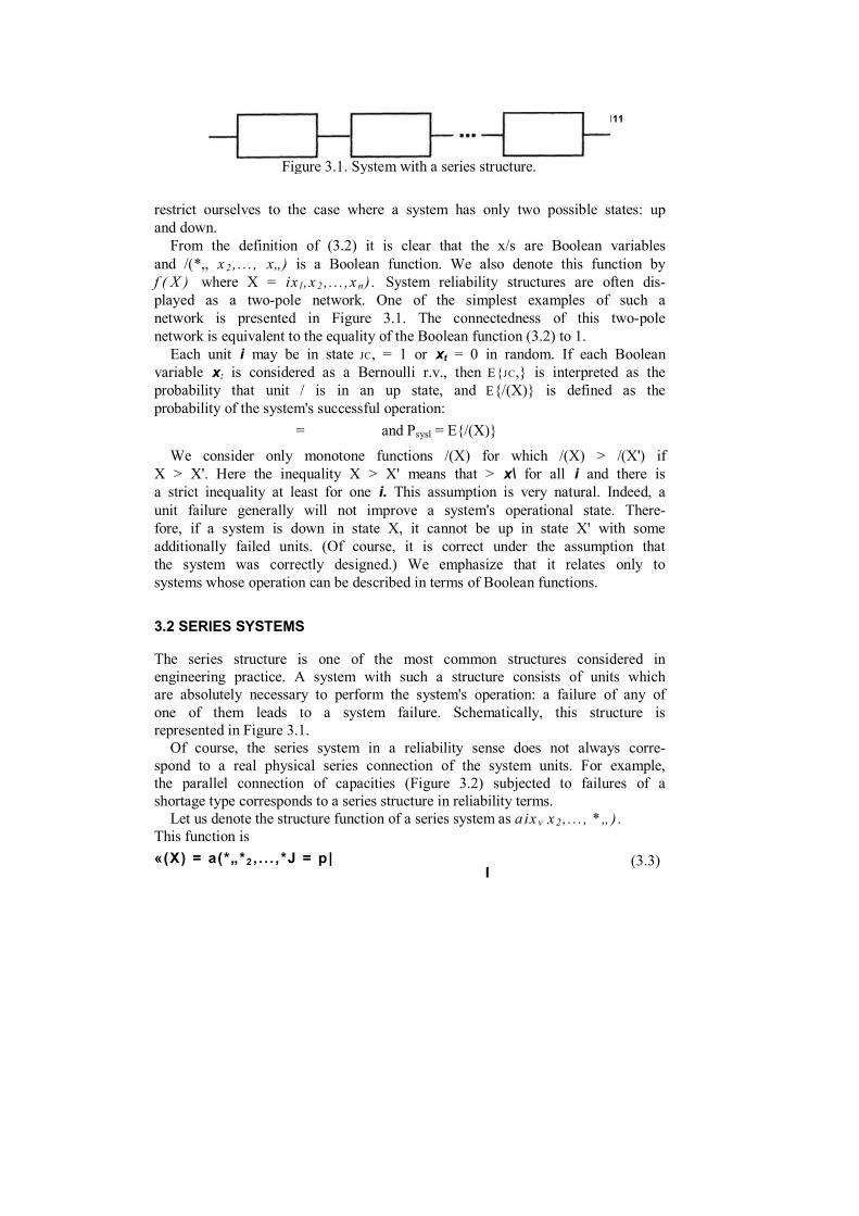
SERIES SYSTEMS 111
restrict ourselves to the case where a system has only two possible states: up and down.
From the definition of (3.2) it is clear that the x/s are Boolean variables and /(*,, x 2 , . . . , x„) is a Boolean function. We also denote this function by f ( X ) where X = ix l ,x 2 , . . . ,x n ) . System reliability structures are often dis- played as a two-pole network. One of the simplest examples of such a network is presented in Figure 3.1. The connectedness of this two-pole network is equivalent to the equality of the Boolean function (3.2) to 1.
Each unit i may be in state JC, = 1 or xt = 0 in random. If each Boolean variable x: is considered as a Bernoulli r.v., then E{JC,} is interpreted as the probability that unit / is in an up state, and E{/(X)} is defined as the probability of the system's successful operation:
= and Psysl = E{/(X)}
We consider only monotone functions /(X) for which /(X) > /(X') if X > X'. Here the inequality X > X' means that > x\ for all i and there is a strict inequality at least for one i. This assumption is very natural. Indeed, a unit failure generally will not improve a system's operational state. There- fore, if a system is down in state X, it cannot be up in state X' with some additionally failed units. (Of course, it is correct under the assumption that the system was correctly designed.) We emphasize that it relates only to systems whose operation can be described in terms of Boolean functions.
3.2 SERIES SYSTEMS
The series structure is one of the most common structures considered in engineering practice. A system with such a structure consists of units which are absolutely necessary to perform the system's operation: a failure of any of one of them leads to a system failure. Schematically, this structure is represented in Figure 3.1.
Of course, the series system in a reliability sense does not always corre- spond to a real physical series connection of the system units. For example, the parallel connection of capacities (Figure 3.2) subjected to failures of a shortage type corresponds to a series structure in reliability terms.
Let us denote the structure function of a series system as a ix v x 2 , . . . , *„) . This function is «(X) = a(*„*2 , . . . , *J = p|
I
Figure 3.1. System with a series structure.
(3.3)

11 6 UNREPAIRABLE SYSTEMS Figure 3.2. A parallel connection of ca- pacitors which represents a series struc- ____ ture in a reliability sense.
where the symbol f| denotes the Boolean product (disjunction). The same expression can be written in an equivalent form
a(X) = min xt
In reliability theory systems consisting of independent units are usually considered. In this case the computation of the probability of a successful system operation is easy. We are interested in the probability
Pr{a(x,, x2,...,x„) = 1} = E{a(x,, x 2 , . . . , x„ ) } (3.4)
For independent units (3.4) might be rewritten in two equivalent ways
pr{ n *, = i } = n pr{x,. = i } = n p, (3.5) Is/f in
e{ n 4 = n e{x(. = 1} = n P, (3.6) 1 SiSn ' 1 1
Expressions (3.5) and (3.6) make the following statements true:
1. A series system's reliability decreases (increases) if the reliability of any unit decreases (increases).
2. A series system's reliability decreases (increases) if the number of units increases (decreases).
3. A series system's reliability is worse than the reliability of any of its units.
The first two statements reflect the monotonicity property.
SERIES SYSTEMS 113 Above we have considered the static case where probabilities are specified as constant. But the process of a system's operation develops over time, so it is reasonable to consider a random function x,(f):
_ j 1 if the ith unit is operating at moment / ~ 10 otherwise * ' )
This function is monotone and nonincreasing over time for unrepairable units; that is, after a failure the unit cannot return to state 1. In other words, jc,(f + A) < x tU) for any A > 0. Thus, for the system as a whole, it follows that /(X(f + A)) </(X(0). From (3.5) it follows that
= n m o
(3.8)
1 sisn
Obviously, (3.5) and (3.8) can be written in a direct way from the verbal definition of a series system's successful operation:
Pr{a series system operates successfully}
= Pr{all system's units are up}
= Pr{unit 1 is up, AND unit 2 is up,..., AND unit n is up}
= Prfunit 1 is up} Pr{unit 2 is up} ... Pr{unit n is up)
In a more general case, direct calculations must be used for obtaining the function P(t) for the system. But in one important particular case, when each Pj(t) is an exponential function, we can write a very simple expression
>W') = n = exp(-< E A,.)=e-A' (3.9) lsisfi v Is/sn '
where
A= E A, 1
Suppose a system consists of highly reliable units: p((r) = 1 - e^t) where Ej(t) is very small; for example,
1 max e ( t ) < K —
Is/sn n

11 6 UNREPAIRABLE SYSTEMS [It is clear that the smallness of for each particular case depends on the number of units.] Then, for a system with units having arbitrary distributions of time to failure,
nvs,(o = n [ i-e,(o]- i- £ « ,(o (3 .io) 1 sis." Uisn
The error of the calculation in this case will not exceed the value
^,(0 - n [1-6,(0] < L e,(0«i(0 < (?)[ max e,(0|2 1 sisn lrsjc/sn V^/tlSiiSn J
(3.11)
Let us consider a particular case. Suppose a series system consists of n units, each of which has a continuous failure distribution with a nonzero first derivative at t = 0. Suppose the system is operating during a small period of time t0 . The Taylor series restricted to the first term is
'o=/(0)'o
( - 0
Note that, at t = 0,
/(0)
m - m - m
Then, for a series system consisting of a large number of highly reliable identical units with an arbitrary d.f. F(t) ,
" [1 - A(0)<o]n - exp[-nA(0)*0]
If the units are different but some of them have distribution functions F)(/), i e a, with nonzero first derivatives at t = 0 equal to A,(0), then for small t0
F ( t )dt
(3.12)
■'oLA,(0) (3.13)P^tCo)~ n(l -A,(0)r0) = exp
Of course, we assumed that |a| » 1; that is, the number of distributions witha nonzero derivative is large. Therefore, we see one more example of anexponential distribution in reliability theory.
SERIES SYSTEMS 115
1
If the distribution of a unit's TTF is such that dFi^/dt' = 0 for i < k and d kFiO) /dt k = a, then
=
[ l ( 3 - 1 4 )
For large n one can write the approximation
where A = na. Thus, this series system has a Weibull-Gnedenko distribu- tion of time to failure. One practical example of such a system concerns a set of bearings in a machine. Another example will be presented in Section 3.4. In the ideal case, if all of the series system's units have a constant TTF, that is, a degenerate distribution of the type
11 if t Tt ^ ^ \ 0 otherwise
then Pit) coincides with the pf(() of the worst unit, that is,
i W ' J - l 1 i f r - m i n r ' (3.16) \ 0 otherwise
Of course, such a distribution does not exist in a real life. (Mathematics always deals with ideal objects!) But normally distributed r.v.'s with very small coefficients of variation can be considered as "almost constant" or "almost nonrandom." Now consider the MTTF of a series system. For any series system the random TTF, say Y, can be expressed through the random TTFs of its units i y t ) in the following way:
Y = min yf
(3.17
)
The MTTF can be found in a standard way as
rsys, = E{y) = j~ysyjt)dt (3.18)
where P^U) is determined above. For an exponential distribution, p/f) = exp(-A,(),
11 6 UNREPAIRABLE SYSTEMS
Tsysl - fexp(-r E A,) dt = 1 = ----------------------------- ------ (3.19) V Isisn ' L. A< V -I
y _ T
where is the MTTF of the ith unit.

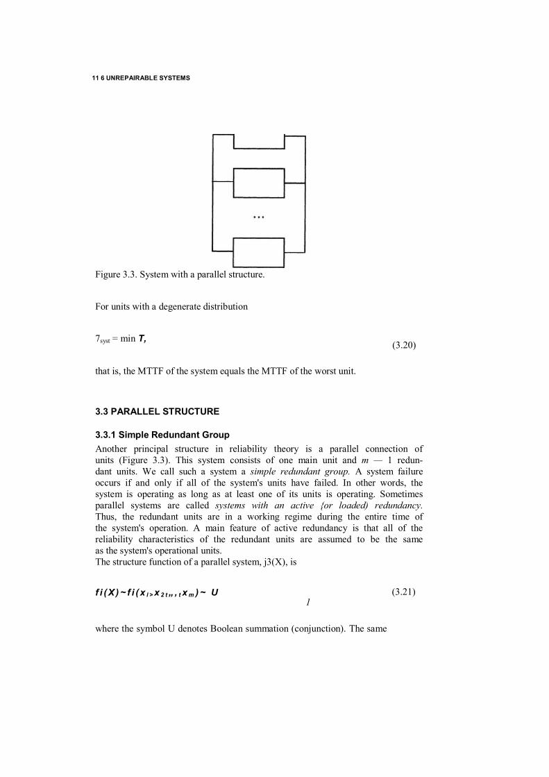
11 6 UNREPAIRABLE SYSTEMS
Figure 3.3. System with a parallel structure.
For units with a degenerate distribution
7syst = min T,
that is, the MTTF of the system equals the MTTF of the worst unit.
3.3 PARALLEL STRUCTURE
3.3.1 Simple Redundant Group Another principal structure in reliability theory is a parallel connection of units (Figure 3.3). This system consists of one main unit and m — 1 redun- dant units. We call such a system a simple redundant group. A system failure occurs if and only if all of the system's units have failed. In other words, the system is operating as long as at least one of its units is operating. Sometimes parallel systems are called systems with an active {or loaded) redundancy. Thus, the redundant units are in a working regime during the entire time of the system's operation. A main feature of active redundancy is that all of the reliability characteristics of the redundant units are assumed to be the same as the system's operational units. The structure function of a parallel system, j3(X), is
f i ( X ) ~ f i ( x l > x 2 t „ , t x m ) ~ U 1
where the symbol U denotes Boolean summation (conjunction). The same
(3.20)
(3.21)
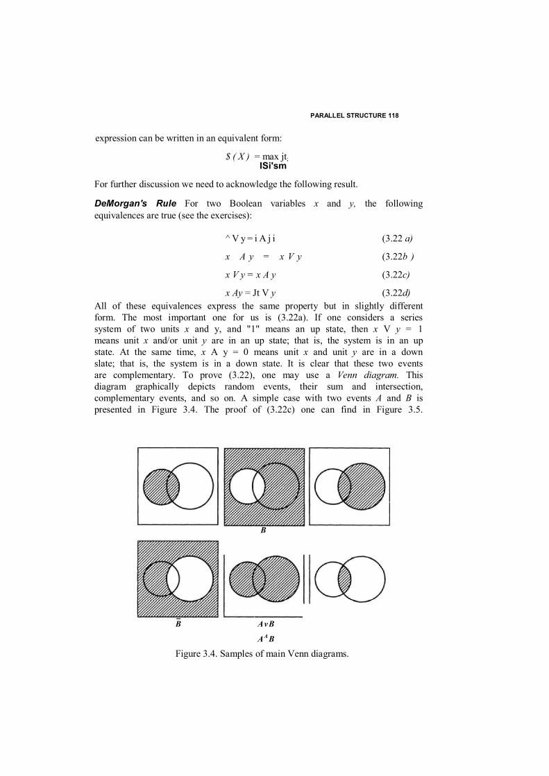
PARALLEL STRUCTURE 118
expression can be written in an equivalent form:
$ ( X ) = max jt; lSi'sm
For further discussion we need to acknowledge the following result.
DeMorgan's Rule For two Boolean variables x and y, the following equivalences are true (see the exercises):
^ V y = i A j i (3.22 a)
x A y = x V y (3.22b )
x V y = x A y (3.22c)
x Ay = Jt V y (3.22d) All of these equivalences express the same property but in slightly different form. The most important one for us is (3.22a). If one considers a series system of two units x and y, and "1" means an up state, then x V y = 1 means unit x and/or unit y are in an up state; that is, the system is in an up state. At the same time, x A y = 0 means unit x and unit y are in a down slate; that is, the system is in a down state. It is clear that these two events are complementary. To prove (3.22), one may use a Venn diagram. This diagram graphically depicts random events, their sum and intersection, complementary events, and so on. A simple case with two events A and B is presented in Figure 3.4. The proof of (3.22c) one can find in Figure 3.5.
B
B AvB
AA B
Figure 3.4. Samples of main Venn diagrams.
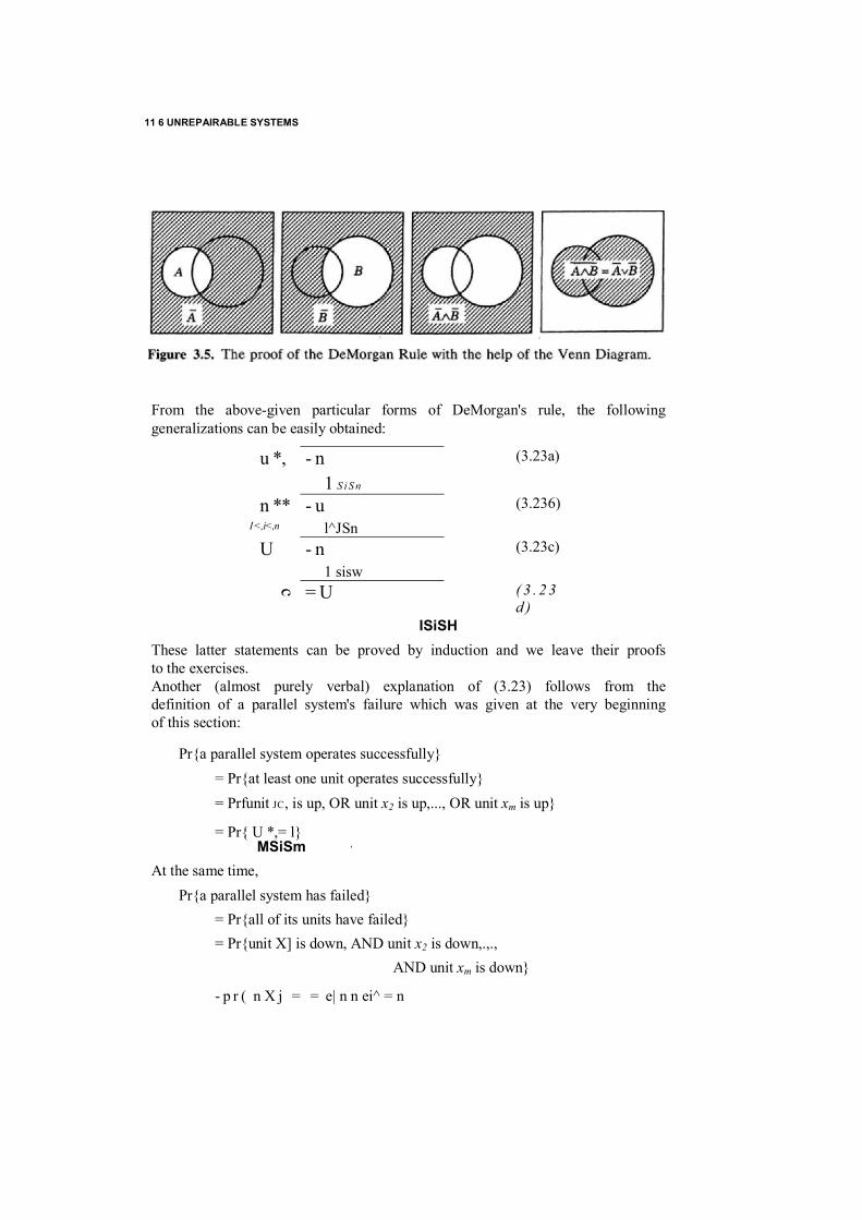
11 6 UNREPAIRABLE SYSTEMS
From the above-given particular forms of DeMorgan's rule, the following generalizations can be easily obtained:
ISiSH These latter statements can be proved by induction and we leave their proofs to the exercises. Another (almost purely verbal) explanation of (3.23) follows from the definition of a parallel system's failure which was given at the very beginning of this section:
Pr{a parallel system operates successfully}
= Pr{at least one unit operates successfully} = Prfunit JC, is up, OR unit x2 is up,..., OR unit xm is up}
= Pr{ U *,= l} MSiSm '
At the same time, Pr{a parallel system has failed}
= Pr{all of its units have failed} = Pr{unit X] is down, AND unit x2 is down,.,.,
AND unit xm is down}
- p r ( n X j = = e| n n ei^ = n
u *, - n (3.23a) 1 S i S n
n ** - u (3.236) I <,i<,n l^JSn
U - n (3.23c) 1 sisw
c = U ( 3 . 2 3d )
PARALLEL STRUCTURE 119
We note that if two events, say z and z, are complementary, then
Pr{ z = 1} + Pr{z = 1} = I
Consequently,
Pr{ U X, - l) - 1 - Pr{ n x A - 1 - n Qi (3.24) Msism ' M stsm ' lzi<.m
Now the equivalence of (3.23) can be confirmed in an inverse way by the equality of the probabilities. We repeat that a detailed inference was done above only from a method- ological viewpoint to provide further discussion. Of course, it was enough to use a verbal definition of a parallel system of independent units and to write the final expression. Sometimes a different form equivalent to (3.24) is used
Psys. = P \ + QlPl + QlQlPl + ' •• +<?1<?2 ....... Qm- \Pm
= Pl + h(Pz + h ( P 3 + • • • ) )
This expression can be explained as follows: Pr{a parallel system operates successfully}
= Pr{the first unit is up, OR if the first unit has failed, the second one
has not failed; OR if both of these units have failed,
then the third one has not failed, OR • ■ • }
If each of the system's units has an exponential TTF distribution, p,(f) = exp(-/A,), for a highly reliable system where max <?,(/) « l/m, one can write <?,(/) = fA(, and, finally,
.C) = 1 II A, (3.25) 1 s/sra
If each unit of a parallel system has a constant time to failure (a degenerate distribution of TTF), then
= (i f° r 'Sm a X 7 ; (3-26) syi,v ' 10 otherwise v '
11 6 UNREPAIRABLE SYSTEMS
Now consider a parallel system's MTTF. For this system the random TTF (£syst) is expressed through the random TTFs of its units (£,) as
£sysl = max & (3.27)
Thus, this is equivalent to the statement that a parallel system operates successfully until the last failure of its units. When each unit has an exponential distribution of TTF, an analytic expression can be derived. For this purpose write the probability of failure- free operation in the form
W')- l - n ( l - e -V ) I <.m
« £ e-V £ + V + £ (.-(Ai + Ay + AtX I I £ i < j s m I £ i < j < k s m
+ (-I)"exp(-r £ A,) (3.28)
ISiSm '
Integrating (3.28) gives
1 T5yS| = £ T( ~~ £
\< . i& m 1 z i< j s m +
+(-1)"—=r --------- (3.29) t - z l< j< k * m A i + A J + £
1
If, at the same time, all units are identical
In this case the MTTF has the form
(3,30)
where T is the MTrF of a single unit. For large m, a well-known approxima- tion for a harmonic set can be applied:
Tsysl « r(ln m + C) (3.31)

PARALLEL STRUCTURE 121
where C is Euler's constant: C = .57712.

11 6 UNREPAIRABLE SYSTEMS
Formula (3.30) can be explained in a simple and understandable way with the use of the memoryless property of the exponential distribution. At the moment t = 0 the system of m active redundant units has a failure rate Am = mA. The first failure occurs in a random time Zm with an exponential distribution with parameter Am. After this failure the system consists of m — 1 units, so its failure rate is now Am_, = (m — 1)A. The second failure occurs in a random time Zm_, with an exponential distribution with parame- ter Am_,. And so on, until the last unit has failed.
The total time of a successful system's operation consists of the sum of all these intervals, that is, Tsysl = E{Z, + Z2 + • • • +Z m) . Obviously, this result coincides with (3.30).
From (3.30) and (3.31) it follows that, at least theoretically, the use of active redundancy potentially allows one to construct a system with an arbitrarily large MTTF value. Of course, one needs to understand that such a mathematical model is strongly idealized. First of all, one must take into account the necessity to use a switching device which itself possesses a nonideal reliability. On the other hand, even with absolutely reliable switch- ing devices, the growth of the system's MTTF is very slow. Several examples are shown in Table 3.1.
Hardly anybody would ever use such redundancy (even with absolutely reliable switches!) to improve the MTTF. But this kind of redundancy can be successfully used if one considers other indexes of reliability, for example, the probability of a system's successful performance. In this case if the initial value of q( t) is much less than 1, each new parallel unit decreases the system's unreliability level by the order q.
Note that for a nonexponentially distributed TTF with an increasing failure rate (i.e., for "aging" units), the growth of a system's MTTF" is even slower.
3.3.2 "k out of n" StructureFor some technical schemes one sometimes considers a special structure—the so-called "/c out of n" structure, or voting system. In engineering practice such a system almost always consists of identical units. In this case the system
TABLE 3.1 Dependence of a System's MTTF on Its Units' MTTF Number of Redundant Units Relative Growth of the System
MTTF 0 1 9 2.88
99 5.18 999 7.48
10'° 23.6

MIXED STRUCTURES 123
operates successfully if at least k out of its total n units are operating. The

11 6 UNREPAIRABLE SYSTEMS
structure function of the system is illustrated here by a simple example with "2 out of 3":
f { x t , x 2 , X 3 ) = A x 2 A jr3 V X ] A x 2 A X3 V JCj A X 2 A JC3 V jcj A x 2 A X 3
(This case is most often encountered in engineering practice.) In general, the structure function of a "k out of n" structure can be written in the form
¥>(X) - l £ ( £ «
where
+ \0 otherwise
We will use an explanation based on combinatorial methods, avoiding the structure function. Considering a "k out of n" structure corresponds to the binomial test scheme, so
Pr {v=j} = J") pJq»-t
and, consequently, the probability of a system's failure-free operation equals Psyst(0 = Pr{^M = L ("W"' 0-32)
puo - i - < k } = \ - z (7W-' (3-33)
For a highly reliable system where q l/n from (3.33) one can easily write
The task of finding the MTTF of such a system for arbitrary unit failure distributions is not simple. One may use any numerical method. The only case where it is possible to obtain an analytical result is the case of the exponential distribution p( t) = exp(-A/). We will not integrate (3.32), but we will use the method described above. The system starts with n operating units and operates, on the average, 1/«A

MIXED STRUCTURES 125
units of time until the first failure. After the first failure, there are n — 1 operating units in the system. They work until the next failure, on the average, 1 /(« - 1)A units of time, and so on until the (k + l)th failure has occurred. Thus, the system's MTTF equals
For an arbitrary distribution p ( t \ one should use a direct numerical integra- tion of PrVM) or a Monte Carlo simulation.
3.4 MIXED STRUCTURES
Pure series or pure parallel systems are rarely encountered in practice. Indeed, mixed structures with series and parallel fragments are common. For example, a duplicate computer system may be used for monitoring a produc- tion line. Each of these two computers, in turn, is represented by a series structure, and so on. A combination of series and parallel structures can generate various mixed structures. First, let us consider "pure" series-parallel and parallel-series types of structures (see Figures 3.6a and 3.7a) because they will be of interest in further discussions. For these structures the following expressions can be easily written. For a parallel-series structure, one has
where
or
(3.34)
where N is the number of units in a series subsystem.
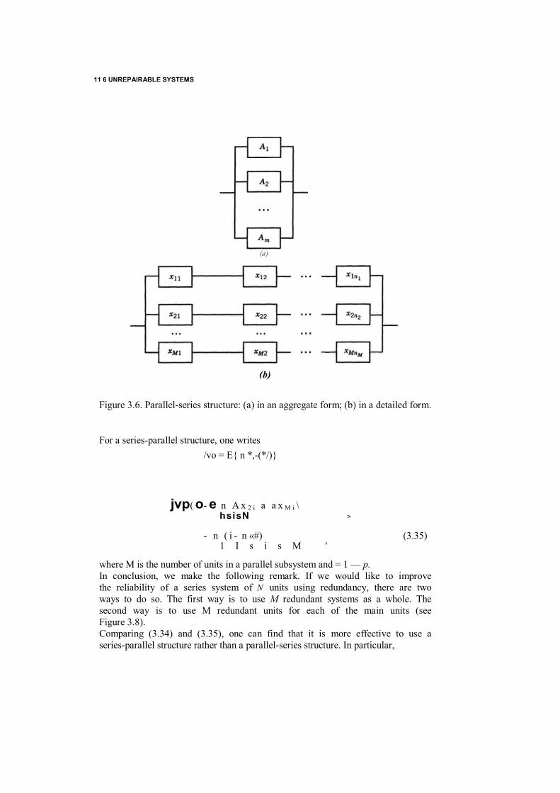
11 6 UNREPAIRABLE SYSTEMS
(b)
Figure 3.6. Parallel-series structure: (a) in an aggregate form; (b) in a detailed form.
For a series-parallel structure, one writes /vo = E{ n *,-(*/)}
jvp( o- e n A x 2 i a a x M i \ hsisN >
- n ( i - n «#) (3.35) 1 I s i s M '
where M is the number of units in a parallel subsystem and = 1 — p. In conclusion, we make the following remark. If we would like to improve the reliability of a series system of N units using redundancy, there are two ways to do so. The first way is to use M redundant systems as a whole. The second way is to use M redundant units for each of the main units (see Figure 3.8). Comparing (3.34) and (3.35), one can find that it is more effective to use a series-parallel structure rather than a parallel-series structure. In particular,
(a)
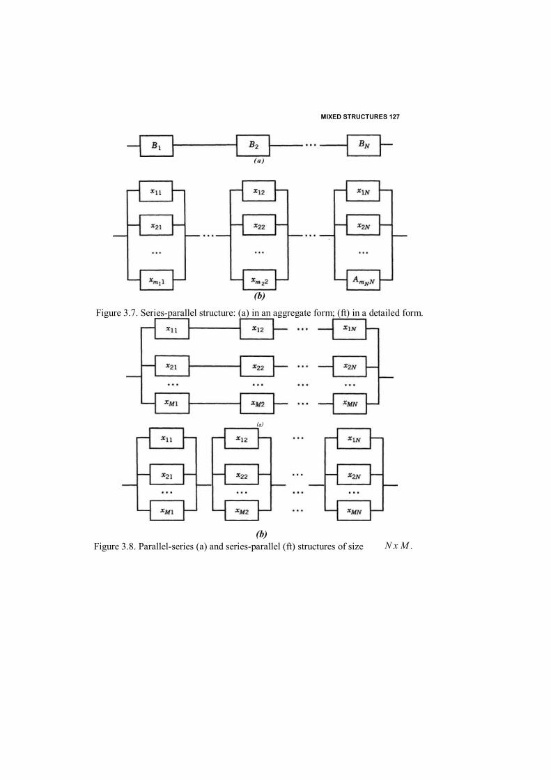
MIXED STRUCTURES 127
(b) Figure 3.8. Parallel-series (a) and series-parallel (ft) structures of size
(a )
(b)
Figure 3.7. Series-parallel structure: (a) in an aggregate form; (ft) in a detailed form.
(a)
N x M .

11 6 UNREPAIRABLE SYSTEMS
for identical units
1 - (I *~PN)M £ (1 - qM)N (3.36) From Figure 3.8 one sees that in a series-parallel system there are more "degrees of freedom," more possibilities to avoid failures. To check this statement, we suggest the extremely simple and clear proof of the statement based on the inequality
max min xu < min max xu (3.37) I sisM IS'SM I
This inequality means that under any splitting of the set of xly.'s by subsets, the minimal value among the maximal values for all these subsets is always larger (not smaller) than the maximal value among the minimal values. Now, using this fact, one can prove the statement. Notice that if is the random TTF of the yth unit in the *'th subsystem of series units, then the random TTF of this subsystem is
fi= min (3.38)
and, consequently, £ps = max ft (3-39)
1 iisJU is the random TTF of the parallel-series system as a whole. Consider the same set divided in such a way that is the random TTF of the jth unit in the ith subsystem of parallel units. Then the random TTF of this subsystem is
max ft, (3.40) 1 S/fim,
and, consequently, £SP = min ft (3.41)
I < . i s N
is the random TTF of the series-parallel system as a whole. A substitution of (3.38) to (3.41) in (3.37) gives, for any sample of r.v.'s ft/f that £SP > £PS. From this it automatically follows that
Tps = eUps} ^ E{£sr} = T s p and
W) = *MfPS P'USP ^ ') - PSPW For a "long" series-parallel system (when N > 1), the Weibull-Gnedenko distribution might be applied if the system's reliability is relatively high. Consider a system of independent identical units. The distribution of the TTF of each parallel subsystem is such that M is the first order of the derivative which differs from 0. As we considered in Section 3.1, in this case
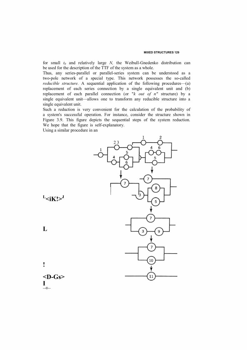
MIXED STRUCTURES 129
for small t0 and relatively large N, the Weibull-Gnedenko distribution can be used for the description of the TTF of the system as a whole. Thus, any series-parallel or parallel-series system can be understood as a two-pole network of a special type. This network possesses the so-called reducible structure. A sequential application of the following procedures—(a) replacement of each series connection by a single equivalent unit and (b) replacement of each parallel connection (or "k out of n" structure) by a single equivalent unit—allows one to transform any reducible structure into a single equivalent unit. Such a reduction is very convenient for the calculation of the probability of a system's successful operation. For instance, consider the structure shown in Figure 3.9. This figure depicts the sequential steps of the system reduction. We hope that the figure is self-explanatory. Using a similar procedure in an
L<iK!>J
L
!
<D-Gs> I —©—
2 3

11 6 UNREPAIRABLE SYSTEMS
Figure 3.9. Examples of the reduction of a complcx structure with parallel and series inner substructures to the simplest kinds of structures.
STANDBY REDUNDANCY 131
inverse way, one can construct various reducible structures from a single equivalent unit by a detailed disaggregation at each step. Examples of irreducible structures (different arbitrary networks) are presented in a later chapter.
3.5 STANDBY REDUNDANCY
A number of systems have standby redundant units. These units are not included in an "active" system's structure. Moreover, these redundant units cannot fail before they occupy an active position. A standby unit instantly replaces its corresponding main unit after the latter's failure. Generally, such a replacement does not occur instantly, but most mathematical models assume that the time of the standby unit's switching into a main position is 0.
The spare parts supply problem is usually analyzed in terms of standby redundancy. For this problem the sufficiency of the stock of spare parts for replacement (or repair performance) is considered rather than the system's successful operation. (Usually, in this case, one considers the inventory system itself. But for simplicity of terminology we will use the terms system failure and instant replacement in further discussion,)
For standby redundancy it is convenient to speak about "a socket" and a set of units which are put into it one by one after each failure. All units for the socket are considered to be identical. In reality, a standby unit of some type must be able to replace the main unit only with a unit of the same type.
3.5.1 Simple Redundant Group If a system consists of a single main unit and m — 1 standby units, we call it a simple redundant group. In this case the random time of the system's successful operation 0m equals
Z i, I 5i<.m
Thus, a system's MTTF can immediately be written as
t <is«
The MTTF does not depend on the switching order of the steady units. If all
Tw = E{9J - E = E m) = E 7] (3.42)

11 6 UNREPAIRABLE SYSTEMS
units of the system are identical,
Tiyst =mT
where T is the single unit's MTTF. Jt is clear that standby redundancy is much more effective than active redundancy: here the growth of rsyst is linear, and for the active redundancy case the growth is only logarithmic. But again we would like to emphasize that this mathematical model is a very idealized picture of reality. Remember the well-known property of the mean: formula (3.42) is valid even if the standby units are dependent. The probability of a system's successful operation Pt(r) can be written as
= ?v{em ^ f} = Pr( E = fM^-, (3.43) ^ Uism '
The system's TTF, = 0in, represents the sum of independent r.v.'s. As we know from Chapter 1, in this case
= 1 - F * m { t ) = f'P^-'Kt - x) d F ( x ) Jo
where P^Jit) is the probability of a failure-free operation of the system with k — 1 standby units (k units in the redundant group). As known from Section 1.3.1, only a very restricted number of d.f.'s allow one to find convolutions in convuluted form. The reader can use the above- mentioned results for probability calculations. Of course, if the number of standby units in the redundant group is large, a normal approximation based on the central limit theorem (see Section 1.3.2) can be used. In engineering practice, especially in electronics, the most frequently used distribution Fi t) is exponential. The standby group's random TTF has an Erlang d.f. of the wth order, and the probability of a failure-free operation is
= E E = E (3.44)
For A( 1 the approximation can be written as
(Af)~ pv«(0 - 1 -------------- r (3.45)
m \
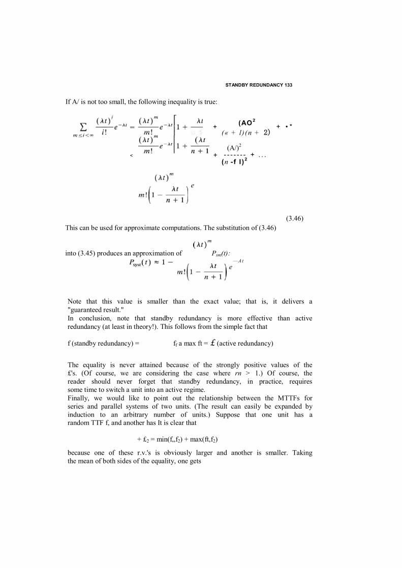
STANDBY REDUNDANCY 133
If A/ is not too small, the following inequality is true:
(AO2
(« + l)(n + 2)
(A/)2 - - - - - - - + . . . (n -f I )2
(3.46)
This can be used for approximate computations. The substitution of (3.46)
into (3.45) produces an approximation of Psm(t): — A t
e
Note that this value is smaller than the exact value; that is, it delivers a "guaranteed result." In conclusion, note that standby redundancy is more effective than active redundancy (at least in theory!). This follows from the simple fact that
f (standby redundancy) = ff a max ft = £ (active redundancy)
The equality is never attained because of the strongly positive values of the £'s. (Of course, we are considering the case where rn > 1.) Of course, the reader should never forget that standby redundancy, in practice, requires some time to switch a unit into an active regime. Finally, we would like to point out the relationship between the MTTFs for series and parallel systems of two units. (The result can easily be expanded by induction to an arbitrary number of units.) Suppose that one unit has a random TTF f, and another has It is clear that
+ £2 = min(f„f2) + max(ft,f2)
because one of these r.v.'s is obviously larger and another is smaller. Taking the mean of both sides of the equality, one gets
+ + • *
n + 1
+ <
e

11 6 UNREPAIRABLE SYSTEMS
E{£, = E{min(f„e2)} + E{max(f„ £2»

STANDBY REDUNDANCY 135 Now we can see that these values are, in order:
* The first is the MTTF of a duplicated system of two standby redundant units which are working sequentially one after another. * The second is the MTTF of a series connection of these units. * The third is the MTTF of a parallel connection of these units.
In particular, when both £'s are exponentially distributed, one can obtain a convenient expression for the MTTF of a parallel system of two different units;
11 1 Tt + ~k2 = Aj + A2 +
or, in final form,
1 1 1 T — _ i ___ _ _______ 1 parallel i v i l
A j A2 A J A 2
Of course, the latter expression has such a simple form only because both distributions are exponential,
3.5.2 "/r out of n" Redundancy The use of standby units for several main units is very common. For example, consider a system which includes k main units. To support the system, there are n - k spare units which can replace any main unit of the group. This method of redundancy is very efficient because of the large number of "degrees of freedom" in the usage of standby units. Indeed, no unit is predetermined to replace some specified main unit. (We repeat that this mathematical model is mainly used to describe a spare units supply system.) For standby redundancy the formulas for P^it) and rsyst cannot be written in a convoluted form except for the case of an exponentially dis- tributed random TTF of the units. We may write the result basing our explanation on simple arguments. Recall again that we assume that the units are independent. The system consists of k identical units and has n - k standby units. The system failure rate equals kA. After a first failure the failed unit is replaced by a redundant unit and the system continues its operation. The random TTF equals r, and has an exponential distribution with parameter k \ . The MTTF in this case equals T/k where T is the MTTF of a single unit. The memoryless property of the exponential distribution and the independence of the units ensure the exponentiality of the system's random TTF. Hence, a random period of a system's successful operation consists of the sum of n — k + 1 i.i.d. TTFs.
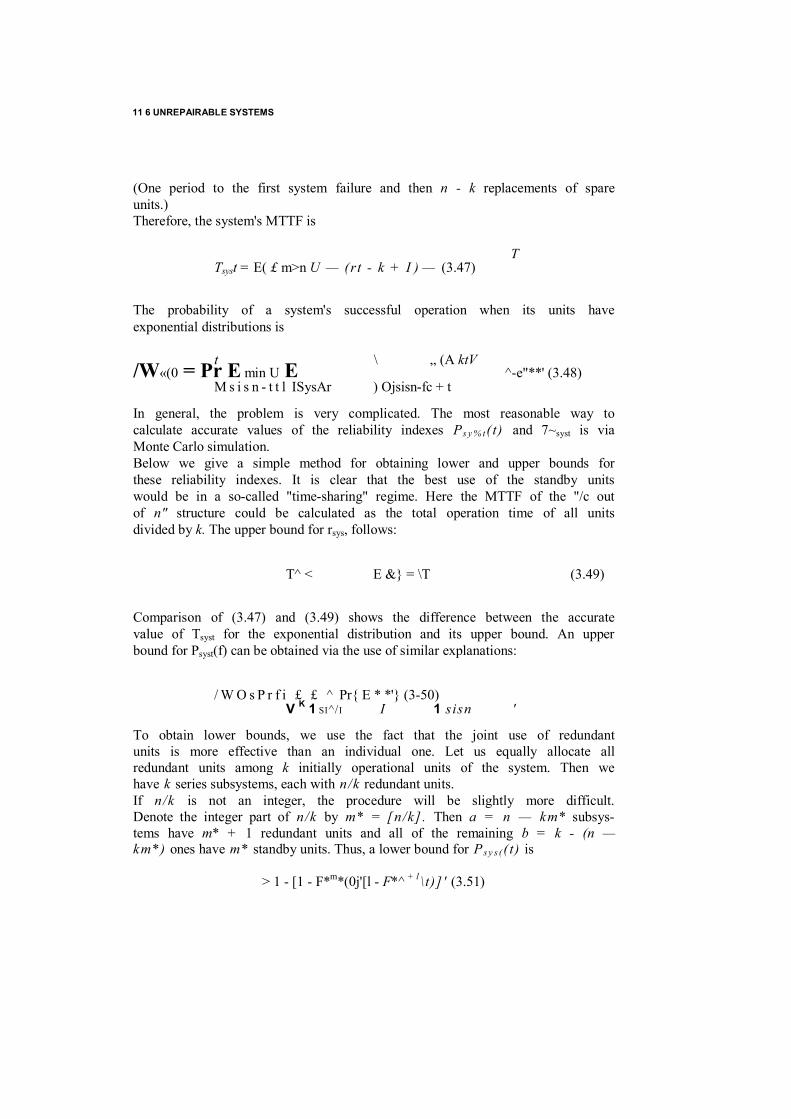
11 6 UNREPAIRABLE SYSTEMS
(One period to the first system failure and then n - k replacements of spare units.) Therefore, the system's MTTF is
T Tsyst = E( £ m>n U — (rt - k + I ) — (3.47)
The probability of a system's successful operation when its units have exponential distributions is
t \ „ (A ktV /W«(0 = Pr E min U E ^-e"**' (3.48) M s i s n - t t l ISysAr ) Ojsisn-fc + t
In general, the problem is very complicated. The most reasonable way to calculate accurate values of the reliability indexes Ps y % t( t) and 7~syst is via Monte Carlo simulation. Below we give a simple method for obtaining lower and upper bounds for these reliability indexes. It is clear that the best use of the standby units would be in a so-called "time-sharing" regime. Here the MTTF of the "/c out of n" structure could be calculated as the total operation time of all units divided by k. The upper bound for rsys, follows:
T^ < E &} = \T (3.49)
Comparison of (3.47) and (3.49) shows the difference between the accurate value of Tsyst for the exponential distribution and its upper bound. An upper bound for Psyst(f) can be obtained via the use of similar explanations:
/ W O s P r f i £ £ ^ Pr{ E * *'} (3-50) V K 1 SI^/I I 1 sisn '
To obtain lower bounds, we use the fact that the joint use of redundant units is more effective than an individual one. Let us equally allocate all redundant units among k initially operational units of the system. Then we have k series subsystems, each with n/k redundant units. If n/k is not an integer, the procedure will be slightly more difficult. Denote the integer part of n/k by m* = [n/k] . Then a = n — km* subsys- tems have m* + 1 redundant units and all of the remaining b = k - (n — km*) ones have m* standby units. Thus, a lower bound for P s y s (( t) is
> 1 - [1 - F*m*(0j'[l - F*^ + l \ t)] ' (3.51)

STANDBY REDUNDANCY 137 where F i t ) is the d.f. of the random TTF of a single unit. A lower bound of the MTTF can be found by integrating (3.51). If the coefficient of variation of Fi t ) is small, (3.51) can be reduced to
where the previous notation is preserved.
3.5.3 On-Duty Redundancy The use of standby redundant units in an operation requires a special regime on duty. This regime is intermediate between the two previously considered types: active and standby.
We illustrate the subject with several examples. An electronic monitor needs at least a portion of a second to be ready to display information. A redundant computer in a control system must be supplied with current information before it is switched to an operational regime. Usually, the unit on duty has a regime which is lighter than the working unit but harder than a total standby one. Practically, there is no realistic input data for this on-duty regime and, moreover, even a confident knowledge about the process is absent. Even with the appropriate input data, the problem of a reliability evaluation in this case is hardly solvable analytically under general assump- tions. As a rule, Monte Carlo simulation allows one to obtain numerical results. But even in this case a lack of input data makes the result very problematic.
The only mathematically acceptable model arises when all units have an exponential distribution of their TTFs: the main ones with parameter A, and the redundant ones with parameter a A where a < 1. In general, a system may have on-duty units which are used for the replacement of failed main units and standby units which are switched into an on-duty position.
Consider a system of k main (operational) units, / on-duty units, and m standby units. Let N = k + I + m. For this case one can build the transition graph in Figure 3.10. On the basis of this graph, the following system of
i t t i t 1 t
N N - l N-m N-m-1 N- m -1 + 1 = ft+1 N-m-1= k
Figure 3.10. Transition graph for an unrepairable system of k main, / on-duty, and m standby units.
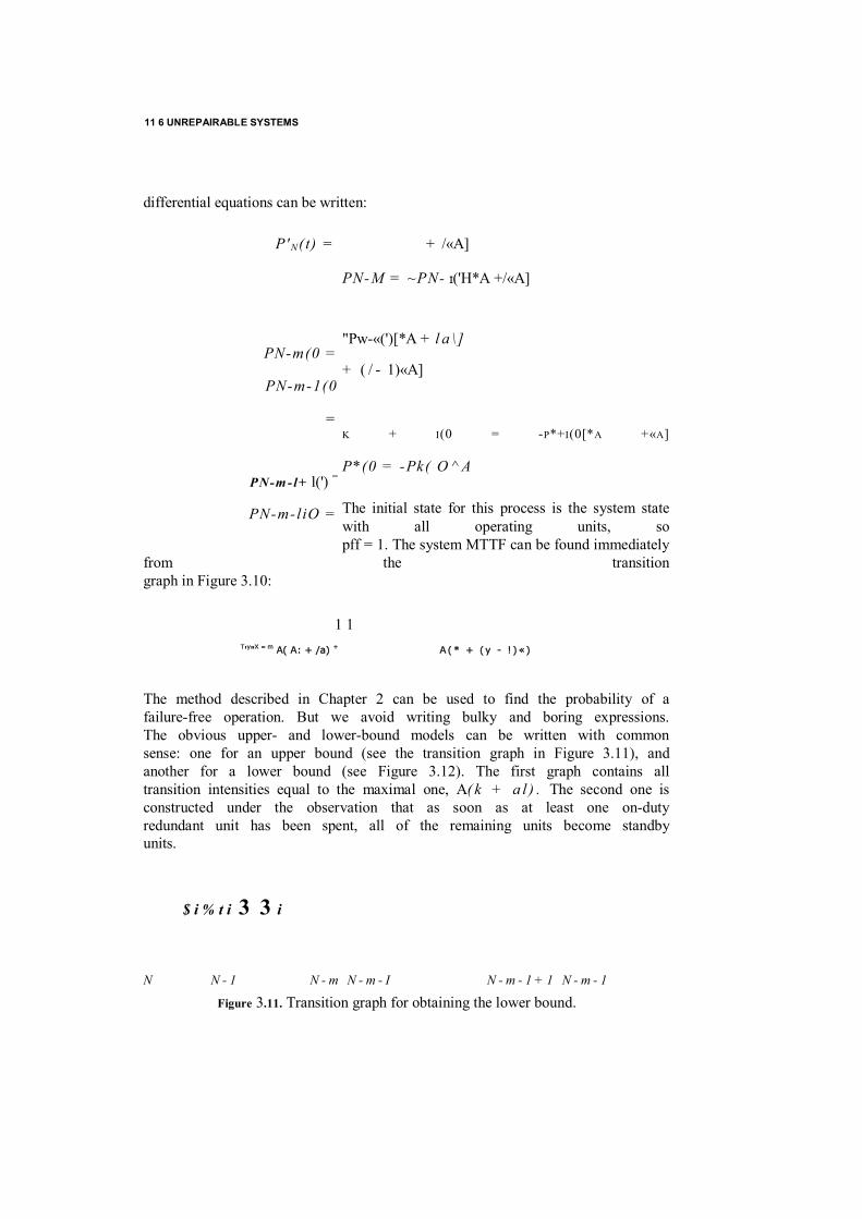
11 6 UNREPAIRABLE SYSTEMS
differential equations can be written:
P' N( t) = + /«A]
PN-M = ~PN- I('H*A +/«A]
"Pw-«(')[*A + l a \ ]
+ ( / - 1)«A]
K + I(0 = -P*+I(0[*A +«A]
P*(0 = -Pk( O ^ A
The initial state for this process is the system state with all operating units, so pff = 1. The system MTTF can be found immediately
from the transition graph in Figure 3.10:
1 1 T'y"X = m A( A: + /a) + A ( * + (y - ! ) «)
The method described in Chapter 2 can be used to find the probability of a failure-free operation. But we avoid writing bulky and boring expressions. The obvious upper- and lower-bound models can be written with common sense: one for an upper bound (see the transition graph in Figure 3.11), and another for a lower bound (see Figure 3.12). The first graph contains all transition intensities equal to the maximal one, A( k + a l ) . The second one is constructed under the observation that as soon as at least one on-duty redundant unit has been spent, all of the remaining units become standby units.
$ i % t i 3 3 i
N N - 1 N - m N - m - I N - m - 1 + 1 N - m - 1
Figure 3.11. Transition graph for obtaining the lower bound.
PN-m(0 =
PN-m-1(0
=
PN-m -l+ l(') =
PN-m-liO =
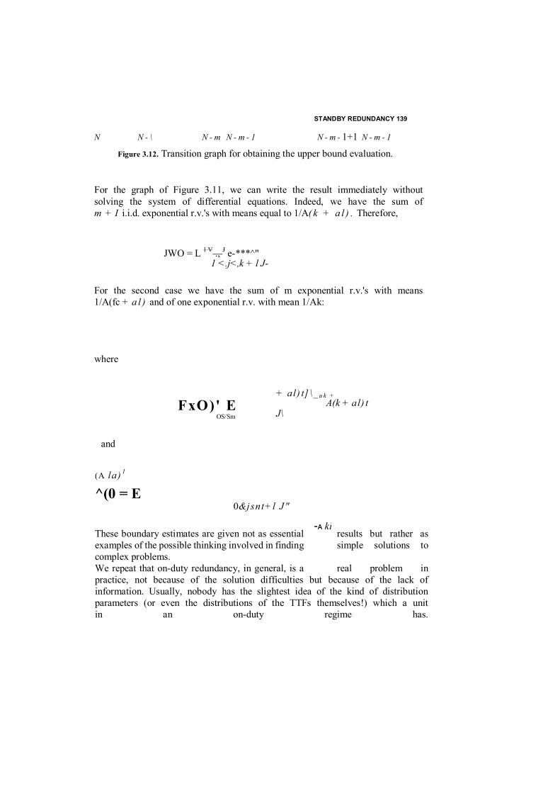
STANDBY REDUNDANCY 139
N N - \ N - m N - m - 1 N - m - 1+1 N - m - 1
Figure 3.12. Transition graph for obtaining the upper bound evaluation.
For the graph of Figure 3.11, we can write the result immediately without solving the system of differential equations. Indeed, we have the sum of m + I i.i.d. exponential r.v.'s with means equal to 1/A( k + a l ) . Therefore,
JWO = L 1 V ., J e-***^" 1 <.j<,k + l J-
For the second case we have the sum of m exponential r.v.'s with means 1/A(fc + a l ) and of one exponential r.v. with mean 1/Ak:
where
+ al) t] \_u k +
A(k + al) t J\
and
(A la) 1
^(0 = E 0&jsnt+l J"
These boundary estimates are given not as essential results but rather as examples of the possible thinking involved in finding simple solutions to complex problems. We repeat that on-duty redundancy, in general, is a real problem in practice, not because of the solution difficulties but because of the lack of information. Usually, nobody has the slightest idea of the kind of distribution parameters (or even the distributions of the TTFs themselves!) which a unit in an on-duty regime has.
FxO)' E OS/Sm
-A ki

11 6 UNREPAIRABLE SYSTEMS
3.6 SWITCHING AND MONITORING
Traditional mathematical models of redundant systems reflect an idealized redundancy: no switching device, no operational monitoring, and no mainte- nance are investigated. These idealized mathematical models help a re- searcher to understand the redundancy phenomenon but they could also lead to very harmful mistakes if these models are used without corrections.
For example, the mathematical formulas show that it is possible to reach any specified level of system reliability with the use of redundant units. But engineering practice convinces us that real system reliability improvement depends on the reliability and quality of the monitoring and switching devices. Both of them are usually far from ideal themselves.
Of course, taking into account all of these various factors will lead to more complex and less elegant mathematical results. But in engineering, the results must be not only elegant but also useful!
3.6.1 Unreliable Common Switching Device In practice, active redundant units are not really operating in parallel. In the case of electronic equipment, the simultaneous presence of several output signals from all redundant units could lead to a real mess. In the case of an information system, the superposition of output information from several computers can produce false signals. Usually, active redundant units are operating in an on-duty regime although their reliability characteristics may not be distinguished from the main unit. All functions of monitoring, switch- ing, and special interface duties are performed by some special device which we call a switching device (SD). Of course, a model of such a group of redundant units almost coincides with the model of a group of active redundant units. But at the same time one needs to take into account the presence of the SD.
Consider a group of m redundant units which uses a common SD for switching from a failed unit to an active redundant one. First of all, note that the SD itself might be one of two main types:
1. The SD is always necessary for the normal operation of the redundant group as a whole.
2. The SD is necessary only at the moment of switching performance.
In the first case, the SD can be, for example, an interface between the redundant group and the remaining equipment. It can be of a various physical nature (electrical, mechanical, hydraulic, etc.). The successful opera- tion of the redundant group depends directly on a failure-free operation of the SD.

SWITCHING AND MONITORING 141
In the second case, the SD becomes necessary only at the moment of switching. Even if the SD has failed, the system can successfully operate until the main unit fails. But then the system will have failed even if there are available redundant units.
Necessary Switching Device Denote the random TTF of the ith unit of the redundant group of m units by ft and the random TTF of the SD by 0 . For the first case, we can write that the random TTF of the redundant group £ is min(0, max ft). For the redundant group as a whole,
= PS D( t)Pm( t) (3.52)
where Pm(t) is the probability of a failure-free operation of the redundant group. In other words, for such an SD, the redundant group can be investi- gated as a simple series-parallel system (see Figure 3.13). The MTTF for this case can be generally found by integrating P^O) as determined in (3.52).
Switching Device Using Only for Switching The second case should be considered in more detail. There arc two possibilities for an SD failure:
1. The SD may fail during the time of the system's operation. 2. The SD may fail with probability Q only at the moment of switching,
independent of the time when it has occurred.
Switching Device Failure Depending on Time Consider a redundant group of identical and independent units with an exponential distribution of their random TTFs. The probability of a successful operation of the redun- dant group is denoted by PR G( t) . The distribution of the switching device TTF FS D( t} is arbitrary. There are two possibilities for the system's opera- tion:
Figure 3.13. Approximate representation of the duplicated system with the switch as a series connection of the two redundant units and a non-ideal switch.
11 6 UNREPAIRABLE SYSTEMS
Notice that both cases—active and standby redundancy—are equivalent, in the sense of the general formula (3.53), under the assumption of exponen- tially of a unit's TTF. These conditions can be written as
PU O^sdWUO + f'PRG{x)e-M'-xydFSD(x) (3.53)
where PSD(0 = l - FSD((). The exponentiality of a unit's TTF permits us to use (3.53) for both active and standby redundancy. The expressions for the redundant group, PRG(t), are different, but the residual time of the remaining unit after an SD failure is exponential in both cases. From (3.53) one sees how the reliability of an SD influences the reliability of the system as a whole. A system's MTTF Tsyst can be obtained only by integrating the correspond- ing P^O). Now we would like to consider some limiting cases. If TnG » TSD, then TsyN( equals 7*RG for all practical purposes. If TRG TSD, then Tsys, approximately equals TSD + T, where T is the MTTF of a single unit.
Example 3.1 Consider a duplicate system with an active redundant unit. The distributions of the random TTFs for the unit and for the SD are exponential with parameters A and ASD, respectively. Find the probability of a failure-free operation during a time interval t:
+ 1 - (1 — e~jkJC)4]e_A(,~*)ASDe~Asi>*dx
This solution can be easily obtained in closed form.
For a unit with an arbitrary TIT" distribution, the solution is not so simple, though its general form does not seem especially awkward. (Very often—in- cluding this case—a "simple" form of a formula hides numerical difficulties which arise during computation!) Consider active redundancy. Assume that the current operating unit of the redundant group is chosen randomly. The residual unit's TTF begins from the moment .r (the SD failure). Equation (3.53) transforms into
W) =^SD(0(X - [«(<>n+JK0j£(i - M-Or'l^y^sDt*)
4 The SD fails at some moment x < t, the redundant group has not
failed until x, and, after this moment, the current main unit does not fail during the remaining time t — x.

SWITCHING AND MONITORING 143
(3.54)
11 6 UNREPAIRABLE SYSTEMS
where p i t ) is the probability of a unit's failure-free operation and q i t ) — 1 - p i t ) .
For a standby redundant group, the expression is slightly bulky: the conditional distribution of the residual time of a unit which appears in the operational position at the moment x depends on the number of failures which have occurred before that moment. We obtain an approximation by considering the process of failures before x as renewal. Then we can write
^syst( 0 ~ f ) ^siandhy RC( 5 )
5 The first unit chosen at random operates without a failure during period t .
SWITCHING AND MONITORING 145
f X p ( x - y ) p ( t - x \ x - y ) d H ( y ) J f i
^Sd( 0 ^standby Rg( 0
+ ( ' f l p { t - y ) d H ( y ) Jo ^o
where //(() is the renewal function, Jn other words, H i t ) d t is the probability that some failure has occurred in the time interval [ t , t + dt} . We use H it) though we observe a finite sequence of r.v.'s but not the point renewal process. We should remark that, for highly reliable systems, this approxima- tion is quite good. Both cases also allow the following approximation:
P^ = p ( t ) + q { t ) P s o ( t ) P^ - n U) (3.56)
where P^' is the system with an SD and a redundant group of size k . This approximation gives a lower bound on the probability of interest because we assume that the SD operates successfully during the entire period t. As a matter of fact, an SD failure may not lead to a system failure.
3.6.2 Common Switching Device with Unreliable Switching Consider an active redundant group of n independent and identical units. The system's successful operation is possible in two situations:
+ I Aland by RC,( X ) '0 dx
dFso(x) (3,55)

11 6 UNREPAIRABLE SYSTEMS
This permits one to write a recurrent relationship in the form
= p ( t ) + R f 'p£-»(t - x \x) d q ( x ) (3.57)
where R is the probability of a successful switching.
For a standby redundant group of m independent and identical units, the system's successful operation is possible in two situations:
1. The first unit chosen at random operates without a failure during period
2. The first unit chosen at random fails at some moment x < t, the SD performs a successful switch, and from this moment on the new system of m — 1 redundant units and SD perform successfully until time t.
This description permits one to write the recurrent relationship
- x ) d q { x ) (3.58)
where P^(t) is the probability of a successful operation of the active redundant group of k units during a time interval f.
3.6.3 Individual Switching Devices We assume that each unit of a redundant group may be chosen to replace a failed main unit at random. After the main unit's failure, an individual SD associated with the next unit in the redundant group may successfully perform the next connection, or it may fail. Assume also that a unit's failure leads to a corresponding SD's failure. The absence of an operating unit with an operating SD leads to the system's failure. As follows from the above description, the SD is necessary for the unit to operate.
Switching Devices That Fail with Time For active redundancy a system operates successfully in the following situations:

SWITCHING AND MONITORING 147
The probability of a system's successful operation can be written as
1
Pi0 + /'[ L *2&t-*\*) (mk *)
1 SM- I
where pit) = pSD(f)p((). For a standby redundant group, the expression is simpler. The following are situations wherein a system operates successfully:
1. The first unit operates successfully. 2. After its failure there is a group of m — 1 redundant units with a
random number of operating SDs; this new system operates successfully during the remaining time. The random number of operating SDs appears because of SD failures during the on-duty regime.
The probability of a system's successful operation can be written as
+ jf'{ Z o * ~ k 6 )[pSD(*)l*[<?sD<*)r-*"1} (3.60)
Of course, (3.59) and (3.60) can be practically utilized only with the aid of a computer.
Switching Devices That Fail at the Time of Switching First, consider an active redundant group. There are again two situations where the system can successfully perform its operation:
6 The first unit operates successfully.
M*) (3.59)j p k ( x ) q ' " - k - \ x )
11 6 UNREPAIRABLE SYSTEMS
that the new system of — k redundant units must successfully operate during the remaining time period t — x.
This verbal description corresponds to the expression
« ( o - p ( o + * / f E ("rMipwi'irf*)]""7-1
•{ E Q kP}&{ t-x\x) \dq{x) (3-61)
where Q = 1 - R. When we consider standby redundancy, the system can successfully oper- ate if:
1. The first unit operates successfully. 2. After its failure at some moment x, there is a group of m — 1 standby
units. In some order we try to switch each of these units to the main position until a first successful switching occurs. The number of at- tempts before success is distributed geometrically with parameter R. After k SDs have failed during switching, a successful attempt occurs (k is random). The new system of m - k - 1 redundant units must successfully operate during the remaining time interval t — x. The appropriate probability is
PZ^pO+ R f ' E Q k P ^ ~ k ~ n ( t - X ) d q ( x ) (3.62) 0 ls*sm-l
The MTTF for both systems can only be found numerically. Note that for the exponential distribution and large m, (3.62) can be approximated by
= (3.63)
and the MTIT can be approximated by
7;ys, = \ (3-64)
Both (3.63) and (3.64) are obtained under the assumption of the correctness of the application of the result of the random summation to exponentially distributed r.v.'s. (Note that in our case we consider a fixed number of Bernoulli trials.)

SWITCHING AND MONITORING 149
This brief review does not, of course, cover the entire theme. There are various cases in practice which lie outside the scope of this material. Our main purpose was to display some inferences in this area and not to give the reader a "cook book."
3.6.4 Periodic Monitoring In this section we do not try to examine the monitoring problem but rather give a simple example of the possible influence of monitoring on a system's reliability. Above we considered a redundant system with the possibility of an instant replacement of a failed main unit by a redundant one. In many practical cases such a situation is unrealistic. In many cases the state of the units, main or redundant, can be checked only at some prespecified mo- ments, usually at periodic intervals.
Consider a simple system consisting of two parallel units and one standby redundant unit which cannot be switched immediately to either of the parallel units. This redundant unit can replace either failed parallel unit only at some predetermined moments t s — sA, s = 1,2,... . At these moments the state of the two parallel units is checked and a failure may be detected. (In other words, the monitoring of the units is not continuous.) All units are assumed identical and independent, and their TTF distributions are assumed exponential with parameter A.
The system is considered to have failed if:
1. Both parallel units have failed inside a period between two neighboring check points, even if there is a standby unit.
2. There are no units operating at some moment.
Consider the probability of a system's failure-free operation during N cycles. For this case the following discrete recurrent equation can be written:
nyst(A0 - 1) + 2pc,[ l - Q ( N - 1)] (3.65)
with Psys,(0) = 1. Here Q ( K ) is the probability of a failure-free operation of two parallel units during K cycles, QiK) = 1 - [1 - pK]2, and p = 1 - e~X A . Equation (3.65) can be solved numerically. For the system's MTTF, one can write
Tml = p 2 [ A + 7^3 + 2pq[A + T2] + qlA* (3.66)
where after a successfully operating cycle of length A the system starts its failure-free operations from the beginning. A cycle with two failures contains a portion of useful time which is denoted by A*. Setting A* = A, we can write
11 6 UNREPAIRABLE SYSTEMS
the approximation
- A + p2T^ + 2pqT2 (3.67)
where T2 is the average number of successful cycles of the two parallel units. We essentially use here the Markov nature of the model. Even in this
simple case we have no strong results in a simple form. But we see that monitoring essentially changes the operation process and, consequently, changes the reliability indexes of the system.
Equations (3.65) and (3.66) are complicated enough to make some quanti- tative conclusions, but wc consider two simple limiting cases. It is clear that A -> 0 leads to the continuous monitoring model, and, hence, the system reverts to a system composed of two active redundant units and one standby redundant unit. Incidentally, the MTTF of such a system equals
1 1 1 2 = 2A + 2A + A = A
If, on the contrary, we assume that A -»■ oo, it means that factually the system has no redundant units at all because they will never be used. In this case rsys( = 3/2A. Thus, for intermediate A's, the value of Tmt lies somewhere between the mentioned values.
It is clear that for a series system of units with an exponentially distributed TTF, it is totally unreasonable to have any redundant group which can be switched only after periodically checking the system's state. (We consider reliability indexes such as the probability of failure-free operation or the MTTF.)
3.7 DYNAMIC REDUNDANCY
This interesting redundancy class is very close to the classical problems of inventory control. Consider a redundant group of n units. A part of them might be used as active and another part as standby. There is a possibility of checking the currcnt state of the active units only at some predetermined moments. Thus, there is no feedback information within the interval between two neighboring check points. The system can be found to be failed at a moment of checking even if there are some standby units available to be used. The following questions arise: How many units should be reasonably switched between two checking moments? How does one refill the active redundant group?
From a qualitative point of view, it is clear that it is not reasonable to switch all redundant units to an active state: the reliability at the first stage of operation will be high but the redundant units will be rapidly spent. To switch a small number into the active redundant group is unreasonable because a system failure can, with a high probability, appear before a current check.

DYNAMIC REDUNDANCY 151
This kind of problem may appear in connection with nonmonitoring technical systems, for example, space vehicles designated for an investigation of the solar system. The time of response can be excessively long, and it becomes impossible to control the situation, so that one needs to find some prior rule of autonomous switching of the redundant units over time without external signals,
A possible solution to the problem is to choose moments of switching spare units into acting positions. We will discuss the problem of finding the optimal moments of switching in Chapter 11. Now we only consider how to calculate the reliability indices for such a system.
We call such a kind of redundancy a dynamic redundancy. We will only investigate dynamic redundancy with exponentially distributed unit ITFs. Ail units are also supposed to be identical and independent.
3.7.1 Independent Stages The system possesses n identical and independent units to perform its function up to some time /0. Then an initial group of units, n0, is installed as an active redundant group and ail remaining units are placed in a standby regime. The duration of the system's operation is divided into k stages. There are moments 0 < T, < T2 < "" < RK < t0 when the new group of standby redundant units are to be switched into an active regime. When we consider independent stages, such switching is performed at some predeter- mined moments. Such a procedure is called a programmed controlled switch- ing. The previous group of units is expelled from the operation with no consideration of their real state. (As a matter of fact, no active units may fail before the beginning of the next stage.) In this case all stages are indepen- dent. Such a situation arises if the deployment of previously used units for use at the next stage is a difficult or even impossible engineering task.
In this simple case the probability of a system's successful operation during a time interval equals
n { l - k W P } (3-68)
where Qjitj) is the probability of a failure-free operation of a single unit. The calculation of a system's MTTF is not very simple in this case. Assume
that a failure of the system occurs at some stage k. This means that the system operates successfully for k — 1 stages and during some random time within the last stage. The A:th stage duration equals Ak = rk — The conditional value of a failure-free operational time during stage k (denote this by Ck) is
f* - { max t, \A k)
11 6 UNREPAIRABLE SYSTEMS
This conditional mean time can be found in the standard way,
f p(x)dx h _________ p( A)
and only the group of units at the last stage operates until complete exhaustion of all redundant units.
Finally, for the system we have
(3.69)
Once can use an approximation by replacing £k> with Ak or one can obtain lower and upper bounds by substituting £k = 0 and (k = A*, respectively.
3.7.2 Possibility of Transferring Units A more interesting and more complicated case arises if one considers the possibility of using all nonfailed units at some stage for the next stage. Of course, in this case it is possible to analyze only the systems whose units have an exponentially distributed TTF. If stage j has a duration A a n d there are m units in the active redundant group (including those from the previous stage), then the probability of a failure-free operation is given by
^j(Aj) = 1 — [l — exp(—AAj)]"' After the first stage of a successful operation, the system has a random number, say y, I <;' < «„ of operating units. These units can be used at the second stage, starting at the moment T, with n2 new units switched in by the prior rule. Thus, the total number of units acting at this stage equals n2 + j. The probability of exactly j units {j > 0) being transferred to the second stage is
i>i~I PWi
where p = 1 — q. If the system performed successfully during the first stage, j units (;' > 0) leave to operate at the sccond stage. At the same time, at moment r,, new n2 units are switched into the system. So, for a two-stage process with « ~ «j + n2 , one can write the probability of interest as
PU*2) = E ("2(+J
(3-70)
m*) =
e (a,) n P(^) E A,. + E{(J} t sis/-! E{ max
V1ii^rti >
J

SYSTEMS WITH DEPENDENT UNITS 153
} I

11 6 UNREPAIRABLE SYSTEMS
Similarly, the expression for a system with three stages can be written as
£ h W - ' £ fBa+y)p5fl2"1+J-'(i-«3"s+') 1 W / 1 \ 5 1
(3.71)
Of course, equations such as (3.71) might be considered as the basis for computational algorithms, not for hand calculations. At the same time, it is possible to write a recurrent equation which could be used for computer calculations:
/'sys«(folnt;»)= £ 7 ^ ' ^ . ( ' o - + ; ; » - » , ) ( 3 - 7 2 ) 1 \ 3 I
Notice that in such systems the most important thing is to define the optimal intervals Ak and the number of units rij that should be switched each time. A simple heuristic solution of this optimization problem is presented in Chapter 13.
3.8 SYSTEMS WITH DEPENDENT UNITS
In the real world different random events and random variables are often "associated" and not independent. For instance, units of a system can be dependent through the system's structure, the functioning environment, the inner state changing, and so on. In all of these situations, reliability usually tends to change in the same way for all units: all of a unit's parameters increase or all decrease. Two r.v.'s X and Y are associated if their covariance is positive:
Cov(*,Y) = Cov(y,^) = E{(*~ E{*})(y- E{>>})} > 0
A stronger requirement for the association of two r.v.'s demands that the inequality
Cow [ f l ( X , Y ) , f 2 ( X , Y ) ] >0
holds, where both /, and f2 are increasing or both are decreasing functions. The vector X = ( X x , X2 , . . . , X n ) consists of associated components if
Cov[/ t(X), /2(X)] £0
A more formal discussion of associated r.v.'s can be found in Barlow and Proschan (1975).

SYSTEMS WITH DEPENDENT UNITS 155
3.8.1 Series Systems Consider a series system of two units. Let x t , i = 1,2, be the indicator function of the ith unit. Suppose the jcf's are associated. For instance, both of them are dependent on the same environmental factor ft; that is, nota- tionally, they are jt,(/|ft) and ;t2(r|ft) for some specified ft. Then for these two units one can write
Pr{x { Ar2 = l ) = Pr{x, = l}Pr{x2 = 1} + p(x l t x 2) (3.73)
where p(jfl5 x 2 ) is the correlation coefficient
This normalized value satisfies the condition — 1 < p <i 1. For n associated r.v.'s it is possible to consider only the case p > 1. From this condition and (3.73), for a series system of two associated units, it follows that
Pr{*, A x2 = 1} > Pr{jc, = l}Pr{ jt2 = 1} (3.74)
This result can be immediately generalized for a series system of n associated units:
= Pr{a(X) = 1} > II P I (3-75)
From (3.75) it automatically follows that for a series system of n associated units:
f II P,i 0 (3-76) ■'O Uisn
Consider the example when each unit of a series system depends on the same factor p, for instance, the temperature. The system is designed for use at two different temperatures, p, and p2. The designer decides to check the probability of a failure-free operation of the series system of n units. For this purpose, the designer arranges for a unit testing under these two conditions. The probabilities of the unit's failure-free operation under these two conditions are /?, and p2 , respectively. The average unit failure-free opera- tion probability equals p = (1/2)(p, + p2) . At a first glance, it is very attractive to try to compute the system reliability index as = p" if we know nothing about the real conditions of the system's use. But let us assume that the first condition appears in practice with fre- quency R , and the second condition appears with frequency Q = 1 - R . (Of course, the frequency R can be considered to be a probability.) Then a
11 6 UNREPAIRABLE SYSTEMS
realistic value of the index is Piyst = Rp" + Qp\. It is easy to check that ^sysi — Avst ■ (To convince yourself in a particular case, do it with n = 2 and R = 1.2.) Of course, the same phenomenon will be observed if one considers more than two different environmental conditions. Another example of a system with associated units is a system operating in a changing regime. Assume that a system operates with probability pk at the k t h regime. Under this regime the system's units have a failure rate equal to \k. It may happen if the system switches from regime to regime periodically (or, perhaps, randomly). In this case
UO = Lpke~x'"' v*
This is larger than
v v* '
So, for a series system we can use the hypothesis of the unit's indepen- dence to obtain a conservative bound on the reliability index of types P ( t ) or T.
3.8.2 Parallel Systems Now consider a parallel system of two associated units. For this system we have
Pr{x x V*2= 1}
= 1 - Prj*! AiJ = 1 - [Pr{5, = 1} ? T { X X = 1} + p ( x u x 2 ) } (3.77)
< 1 - Pr{JE, = 1} Pr{Jt, = 1} = 1 - fl,(r)*2(0
where p ( x t , x 2 ) is the correlation coefficient for the indicator functions. It is easy to show that
- V a r ^ V a r K) ^
But Cov(x,, x 2 ) = OM xy , jc2) and Varfx,} = Var{jef}, i = 1,2. Equation (3.78) can immediately be generalized for a parallel system of m associated units:
Psyst - Pr{/3(X) - 1} £ 1 - n 4, (3.79) 1 sism
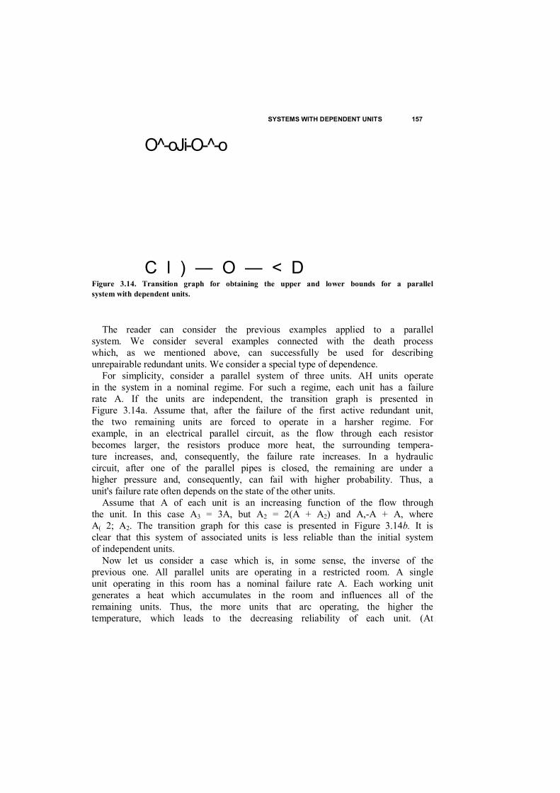
SYSTEMS WITH DEPENDENT UNITS 157
O -oJi-O- -o
C l ) — O — < D Figure 3.14. Transition graph for obtaining the upper and lower bounds for a parallel system with dependent units.
The reader can consider the previous examples applied to a parallel system. We consider several examples connected with the death process which, as we mentioned above, can successfully be used for describing unrepairable redundant units. We consider a special type of dependence.
For simplicity, consider a parallel system of three units. AH units operate in the system in a nominal regime. For such a regime, each unit has a failure rate A. If the units are independent, the transition graph is presented in Figure 3.14a. Assume that, after the failure of the first active redundant unit, the two remaining units are forced to operate in a harsher regime. For example, in an electrical parallel circuit, as the flow through each resistor becomes larger, the resistors produce more heat, the surrounding tempera- ture increases, and, consequently, the failure rate increases. In a hydraulic circuit, after one of the parallel pipes is closed, the remaining are under a higher pressure and, consequently, can fail with higher probability. Thus, a unit's failure rate often depends on the state of the other units.
Assume that A of each unit is an increasing function of the flow through the unit. In this case A3 = 3A, but A2 = 2(A + A2) and A,-A + A, where A( 2; A2. The transition graph for this case is presented in Figure 3.14b. It is clear that this system of associated units is less reliable than the initial system of independent units.
Now let us consider a case which is, in some sense, the inverse of the previous one. All parallel units are operating in a restricted room. A single unit operating in this room has a nominal failure rate A. Each working unit generates a heat which accumulates in the room and influences all of the remaining units. Thus, the more units that arc operating, the higher the temperature, which leads to the decreasing reliability of each unit. (At

11 6 UNREPAIRABLE SYSTEMS
the same time, remember that the system is a parallel system!) We begin the analysis of the transition graph for this case with state 1.
A single unit operates with A, = A, When two units are operating, the temperature in the room is higher and, consequently, A2 = 2(A + A*). When all three units are operating, A3 = 3(A + A*). Under the conditions of the example, A* < A*. The transition graph for this case is shown in Figure 3.14c.
A comparison of these two cases with the initial system of independent units shows that both of them possess a less favorable reliability index than the initial system: in each case the transition intensities are higher than in the initial case. Thus, on average, systems with associated units reach a failure
state more quickly. We finish this comparison with a comparison of the MTTFs:
1 1 1 1 1 1 3 A + 2 A + A " 3 A + 2(A + A2) + A + A,
1 1 1 1 1 1 3A + 2A + A ~ 3{A + A*2) + 2(A + A*) + A
3.8.3 Mixed Structures We consider this concept in more detail in Chapter 9 when we address two-pole network bounds. Here we only illustrate some kind of dependence between the system's units when the system has a mixed structure. Consider the simplest series-parallel and parallel-series systems with different forms of unit dependence. To perform its operation, the system should have at least one unit of type A and at least one unit of type B. Assume that we analyze a system whose two units (say functional blocks) have their own power supply (PS). The power supply is not absolutely reliable. Of course, a power supply failure leads to an immediate failure of both units which are supplied by this PS.
First, consider a series-parallel system. There are two possibilities of switching the power supply (see Figure 3.15). Denote the probabilities of a successful operation by pA , pB , and pP S . Then for structure (a) we can write
Pa =pU[l - (1 -pApB) 2 \ + 2Pp sq v s PA PB
and for structure (fo) we can write
P 6 = P 2PS[ I - ( 1 ~PA PB f \
It is obvious that structure (a) is better than structure (b) .
T - syst
and
T = J syst

TWO TYPES OF FAILURES 159
Now consider two variants of the parallel-series structure (see Figure 3.16). For structure (c) we have
K =PPSO ~ ~ <ll) + 2Pps1PSPAPB
and for structure ( d ) we have
Again, we can deduce that P c > P d without calculation, based only on our previous knowledge about the reliability of a series system with associated units. A consideration of these examples shows us that the reliability of some auxiliary units may have an influence on other system units in such a way that the reliability of a parallel-series structure might be worse than the reliability
Figure 3.15. Two variants of the power supply of a series-parallel structure.
Figure 3.16. Two variants of the power supply of a parallel-series structure.
11 6 UNREPAIRABLE SYSTEMS
of a series-parallel structure. Indeed, it is possible that for some fixed pA, pB , and p PS, for instance, the inequality pa > pd is true:
P p s I 1 - (.1-PAPB)*\ + IPpsIPSPAPB > PP^ 1 " " 1B)
Avoiding general deductions, take pA = pB — p. Denote for simplicity p PS = /i and <2 = 1 — /?. Then the condition
/?2[l - (1 - p2) 2] + 2P<2P2 > «2(1 " Q1) 2
is equivalent to
( i - 0 2 - [ i - 0 -P2 ) 2} R2 > 2p2
The right part of the inequality is restricted by 1 for any p . Thus if Q > R2
this inequality holds for any p. The solution of the corresponding equality gives
3 ± y/5 Q « ----- ---- a 0.382
In other words, for an unreliable common unit (in our case the power supply), with a reliability index lower than approximately 0.6, one should choose a parallel-series structure rather than a series-parallel one. For some additional examples of the analysis of systems consisting of dependent units, see Gnedenko, Belyaev, and Solovyev (1969).
3.9 TWO TYPES OF FAILURES
Some units have two types of failures. For instance, a resistor may be disconnected (leaving an open circuit) in an electric circuit, and in this case no flow goes through the unit. Or it may burn out, and so will not provide any resistance at all (a short circuit). One observes an analogous effect with capacitors: no capacity at all (a short circuit) or infinite capacity (disconnec- tion). In pipelines, holes allow the leaking of pumped liquid, which decreases the user's consumption and, simultaneously, decreases the hydraulic resis- tance. Rubbish in the pipe results in the same decrease in user consumption, but, at the same time, increases the hydraulic resistance. In a most essential way, this phenomenon appears in relay circuits. These circuits are assigned for connection and disconnection and the nature of their failure can be one of two kinds: they may fail to connect or they may fail to disconnect. Each unit (relay) itself is subjected to two similar failures. It
TWO TYPES OF FAILURES 161
makes the problem of redundancy of such systems more difficult: a parallel structure of relays fails if at least one unit makes a false connection when it should be disconnected, and a series structure fails if at least one unit causes a false disconnection when it should be connected. As a matter of fact, mixed series-parallel (parallel—series) structures are more effective in this case. Moreover, for a relay with known probabilities of failure of both types, there is an optimal mixed structure. We consider this problem separately in Chapter I I . Consider a parallel-series relay system. This system can be considered as a two-pole network with an input on the left and an output on the right. Each unit of the system at any moment of time can be in one of three jointly exclusive possible states: failure-free with probability p , failed in a "con- nected" state with probability c, or failed in a "disconnected" state with probability d. First, we consider the case where the system must provide a connection between the input and output. For each series circuit of n units, the probability of a successful connection Rcon can be written as
t f t o n = ( p + c ) n (3.80)
and, for the system as a whole,
„ = i - ( i - *con ) m -1 - [ i ~ ( p + oT (3-8])
If the system must provide a disconnection, the corresponding probabilities
1 - < 1 - / > - < * ) " = 1 - C (3.82)
and
PdlsCon = [1 ~ cT (3-83)
A relay system operation consists of alternating cycles of connections and disconnections. It seems that for this system it is reasonable to choose a reliability index in the form
Psyst = min(FC(m,F[Jiscon) (3.84)
It is clear that a single relay with the same parameters can perform successfully in both cases only with probability p. (Any kind of failure makes one of the operations totally impossible.)
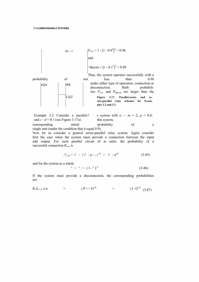
11 6 UNREPAIRABLE SYSTEMS
Pcon = 1 - [1 - 0.92]2 = 0.96
and
^discon = [l ~ 0.12]2 = 0.98
Thus, the system operates successfully with a probability of not less than 0.96
under either type of operation: connection or disconnection. Both probabili- ties Pcon and Pdjscon are larger than the
corresponding initial probability of a single unit (under the condition that it equal 0.9). Now let us consider a general series-parallel relay system. Again consider first the case when the system must provide a connection between the input and output. For each parallel circuit of m units, the probability of a successful connection Rcon is
/?con = 1 - ( 1 - p - c ) m = 1 - d m (3.85)
and for the system as a whole ^ = ^ = ( 1 - ^ ) " (3-86)
If the system must provide a disconnection, the corresponding probabilities are
K d i s C o n = ( P + < O m = ( l - O m
-0—>
Figure 3.17. Parallel-series and se-ries-parallel relay schemes for Exam-ples 3.2 and 3.3.
s system with n — m = 2, p = 0.8,this system,
r@n r€h
L@J
Example 3.2 Consider a parallel-! and c - d = 0.1 (see Figure 3.17a).
(3.87)
MIXED STRUCTURES W!TH PHYSICAL PARAM ETERS 163
and
/,discon = l - [ l " ( / > + < O T
Again wc can use (3.84) to characterize the system as a whole. Again in this case a single relay with the same parameters can perform successfully in both cases only with probability p.
Example 3.3 Consider a system with n = m = 2, p = 0.8, and c = d = 0.1 (see Figure 3.17£>). For this system,
Pcon = 1 - [l - 0.12]2 « 0.98
and
^discon " [1 - 0-92]2 = 0.96
Thus, the system operates successfully with a probability of not less than 0.96 under either type of operation: connection or disconnection. Again both probabilities Pcon and Pdiscon are larger than the corresponding initial proba- bility of a single unit. One can notice that the structures of Figures 3,17a and b are "mirror images" with respect to the probabilities c and d. Thus, both structures are equivalent for the relay with c — d.
3.10 MIXED STRUCTURES WITH PHYSICAL PARAMETERS
A unit presented with an indicator function xt reflects a "dichotomic" object which can only be one of two states: for reliability problems they are termed "success" and "failure." But sometimes we need to analyze systems consist- ing of units with physical parameters whose particular value plays an essen- tial role. In Chapter 1 we introduced the generalized generating sequence (GGS). Here we use it and make some concrete additions to the general method. These additions are helpful for the designing of appropriate computer algorithms. We present the discussion via simple examples.
Series System This case has been considered in Chapter 1. Thus, we consider only simple examples.
Example 3.4 Consider an oil pipeline consisting of n pipes (units) con- nected in series. Each unit has a random capacity which decreases for different reasons: the accumulation of so-called "heavy" fractions on the pipe
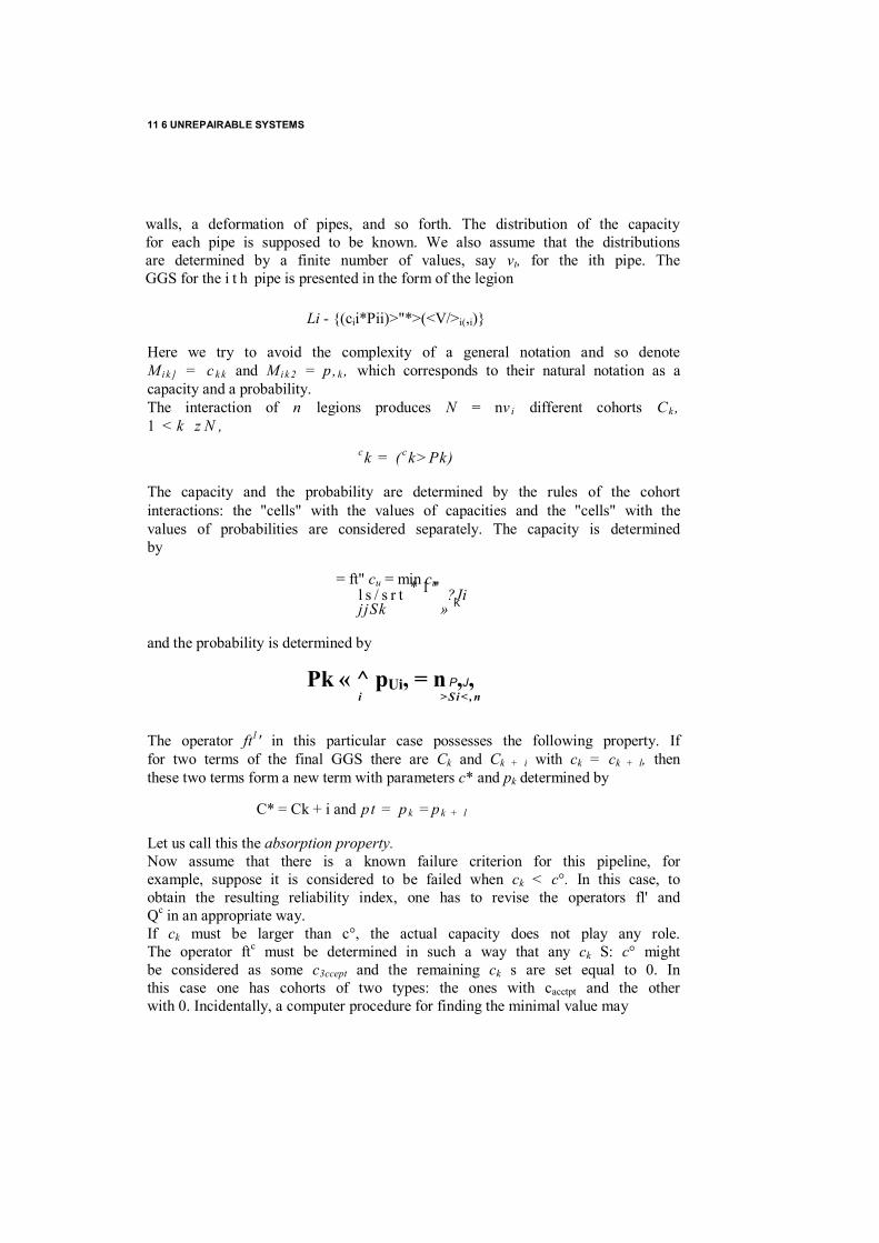
11 6 UNREPAIRABLE SYSTEMS
walls, a deformation of pipes, and so forth. The distribution of the capacity for each pipe is supposed to be known. We also assume that the distributions are determined by a finite number of values, say vt, for the ith pipe. The GGS for the i t h pipe is presented in the form of the legion
Li - {(cii*Pii)>"*>(<V/>i(,i)}
Here we try to avoid the complexity of a general notation and so denote M i k ] = c k k and M i k 2 = p, k , which corresponds to their natural notation as a capacity and a probability. The interaction of n legions produces N = nv i different cohorts Ck , 1 < k z N ,
ck = ( ck>Pk)
The capacity and the probability are determined by the rules of the cohort interactions: the "cells" with the values of capacities and the "cells" with the values of probabilities are considered separately. The capacity is determined by
= ft" cu = min cu * 1 '' l s / s r t ?Ji j jSk » K
and the probability is determined by
Pk « ^ pUi, = n P,J, i > Si< , n
The operator ft1' in this particular case possesses the following property. If for two terms of the final GGS there are Ck and Ck + i with ck = ck + l, then these two terms form a new term with parameters c* and pk determined by
C* = Ck + i and pt = p k =p k + l
Let us call this the absorption property. Now assume that there is a known failure criterion for this pipeline, for example, suppose it is considered to be failed when ck < c°. In this case, to obtain the resulting reliability index, one has to revise the operators fl' and Qc in an appropriate way. If ck must be larger than c°, the actual capacity does not play any role. The operator ftc must be determined in such a way that any ck S: c° might be considered as some c3ccept and the remaining ck s are set equal to 0. In this case one has cohorts of two types: the ones with cacctpt and the other with 0. Incidentally, a computer procedure for finding the minimal value may
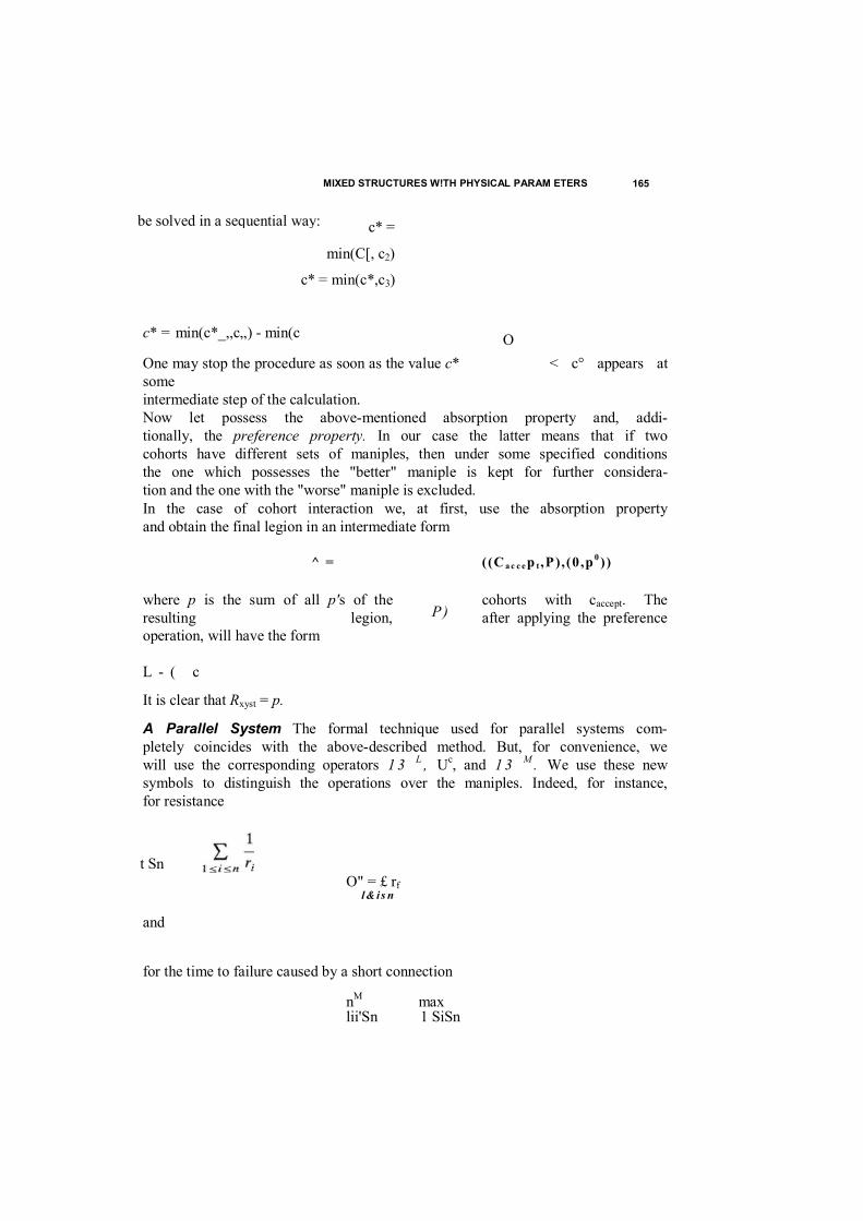
MIXED STRUCTURES W!TH PHYSICAL PARAM ETERS 165
c* =
min(C[, c2)
c* = min(c*,c3)
c* = min(c*_,,c„) - min(c
One may stop the procedure as soon as the value c* < c° appears at some intermediate step of the calculation. Now let possess the above-mentioned absorption property and, addi- tionally, the preference property. In our case the latter means that if two cohorts have different sets of maniples, then under some specified conditions the one which possesses the "better" maniple is kept for further considera- tion and the one with the "worse" maniple is excluded. In the case of cohort interaction we, at first, use the absorption property and obtain the final legion in an intermediate form
^ = ((C a c c ep t ,P), (0 ,p 0 ))
where p is the sum of all p's of the cohorts with caccept. The resulting legion, after applying the preference operation, will have the form
L - ( c
It is clear that Rxyst = p.
A Parallel System The formal technique used for parallel systems com- pletely coincides with the above-described method. But, for convenience, we will use the corresponding operators 1 3 L , Uc, and 1 3 M . We use these new symbols to distinguish the operations over the maniples. Indeed, for instance, for resistance
O" = £ rf l& is n
and
for the time to failure caused by a short connection
nM max lii'Sn 1 SiSn
P)
t Sn
O
be solved in a sequential way:
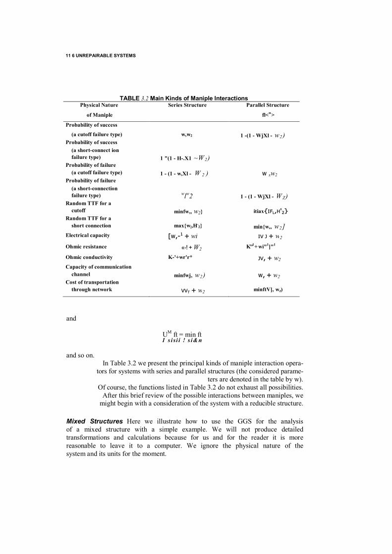
11 6 UNREPAIRABLE SYSTEMS
and
UM ft = min ft 1 s i si i ! s i&n
and so on. In Table 3.2 we present the principal kinds of maniple interaction opera-
tors for systems with series and parallel structures (the considered parame- ters are denoted in the table by w).
Of course, the functions listed in Table 3.2 do not exhaust all possibilities. After this brief review of the possible interactions between maniples, we
might begin with a consideration of the system with a reducible structure.
Mixed Structures Here we illustrate how to use the GGS for the analysis of a mixed structure with a simple example. We will not produce detailed transformations and calculations because for us and for the reader it is more reasonable to leave it to a computer. We ignore the physical nature of the system and its units for the moment.
TABLE 3.2 Main Kinds of Maniple Interactions Physical Nature Series Structure Parallel Structure
of Maniple fl<w>
Probability of success
(a cutoff failure type) w,w2 1 -(1 - WjXl - w2 ) Probability of success
(a short-connect ion
failure type) 1 "(1 - H-.X1 ~W 2)
Probability of failure
(a cutoff failure type) 1 - (1 - w,Xl - W 2 ) W xw2 Probability of failure
(a short-connection
failure type) wlw2 1 - (1 - WjXl - WZ) Random TTF for a
cutoff minfw,, w2} itiax{IFL,H'2} Random TTF for a
short connection max{w],H,2} min{w,, w2]
Electrical capacity [W,-1 + wi IV J + w2
Ohmic resistance «-! + W2 K"1 + wi"1]"1
Ohmic conductivity K-'+wr'r* JV, + w2 Capacity of communication
channel minfwj, w2 ) W, + w2 Cost of transportation
through network VVT + w2 minftV], wz)
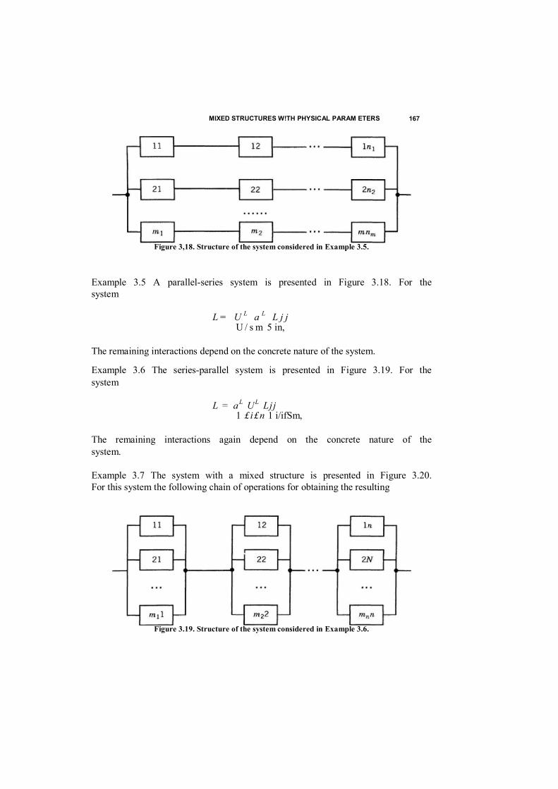
MIXED STRUCTURES W!TH PHYSICAL PARAM ETERS 167
Example 3.5 A parallel-series system is presented in Figure 3.18. For the system
L = U L a L L j j U / s m 5 in,
The remaining interactions depend on the concrete nature of the system.
Example 3.6 The series-parallel system is presented in Figure 3.19. For the system
L = aL UL Ljj 1 £i£n 1 i/ifSm,
The remaining interactions again depend on the concrete nature of the system.
Example 3.7 The system with a mixed structure is presented in Figure 3.20. For this system the following chain of operations for obtaining the resulting
Figure 3,18. Structure of the system considered in Example 3.5.
Figure 3.19. Structure of the system considered in Example 3.6.
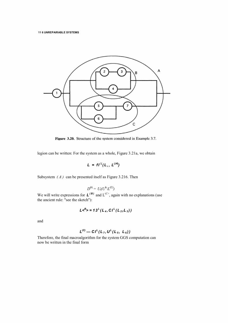
11 6 UNREPAIRABLE SYSTEMS
legion can be written: For the system as a whole, Figure 3.21a, we obtain
L = f l / j ( L , , L(J4))
Subsystem ( A ) can be presented itself as Figure 3.216. Then
DA) = Ul(Ub\L(C))
We will write expressions for L ( B ) and L(C>, again with no explanations (use the ancient rule: "see the sketch"):
L<B> = 13 L ( L 4 , C l L ( L 2 t L 3 ) )
and
L(C) — C I L ( L 7 , U L ( L 5 , L 6 ) ) Therefore, the final macroalgorithm for the system GGS computation can now be written in the final form
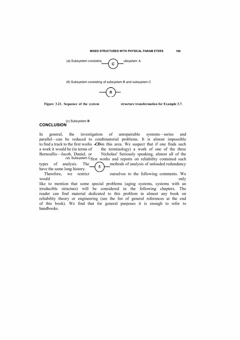
MIXED STRUCTURES W!TH PHYSICAL PARAM ETERS 169
Figure 3.21. Sequence of the system structure transformation for Example 3.7.
CONCLUSION
In general, the investigation of unrepairable systems—series and parallel—can be reduced to combinatorial problems. It is almost impossible to find a track to the first works in this area. We suspect that if one finds such a work it would be (in terms of the terminology) a work of one of the three Bernoullis—Jacob, Daniel, or Nicholas! Seriously speaking, almost all of the
first works and reports on reliability contained such types of analysis. The methods of analysis of unloaded redundancy have the same long history.
Therefore, we restrict ourselves to the following comments. We would only like to mention that some special problems (aging systems, systems with an irreducible structure) will be considered in the following chapters. The reader can find material dedicated to this problem in almost any book on reliability theory or engineering (see the list of general references at the end of this book). We find that for general purposes it is enough to refer to handbooks.
(a) Subsystem consisting of unit 1 and subsystem A
(6) Subsystem consisting of subsystem B and subsystem C
(c) Subsystem B
-CD-
(d ) Subsystem C

EXERCISES 170
REFERENCES
Barlow R. E.,and F. Proschan (1975). Statistical Theory of Reliability and Life Testing.
New York; Holt, Rinehart and Winston. Gncdcnko, B. V., Yu. K. Belyacv, and A. D. Solovyev (1969). Mathematical Methods in Reliability Theory. San Diego: Academic Press.
Kozlov, B. A., and I. A. Ushakov (1970). Reliability Handbook. New York: Holt, Rinehart, and Winston.
Ushakov, I. A., ed. (1985). Reliability of Technical Systems: Handbook (in Russian).
Moscow: Radio i Sviaz.
Ushakov, I. A., ed. (1994). Handbook of Reliability Engineering. New York: Wiley.
EXERCISES
3.1 Prove (3.22a) using the Venn diagram.
3.2 Prove (3.22i>), (3.22c), and (3.22*/) on the basis of the result of Exercise 3.1. {Hint: Use the "double rejection" rule of Boolean algebra: x =x.)
3.3 Prove identities from (3.23 a) to (3.23 d).
3.4 Write the Boolean function tpiX^ for the scheme depicted in Figure E.3.2.
3.5 Write the Boolean function <p{X,) for the scheme depicted in Figure E3.3.
Figure E3.2.
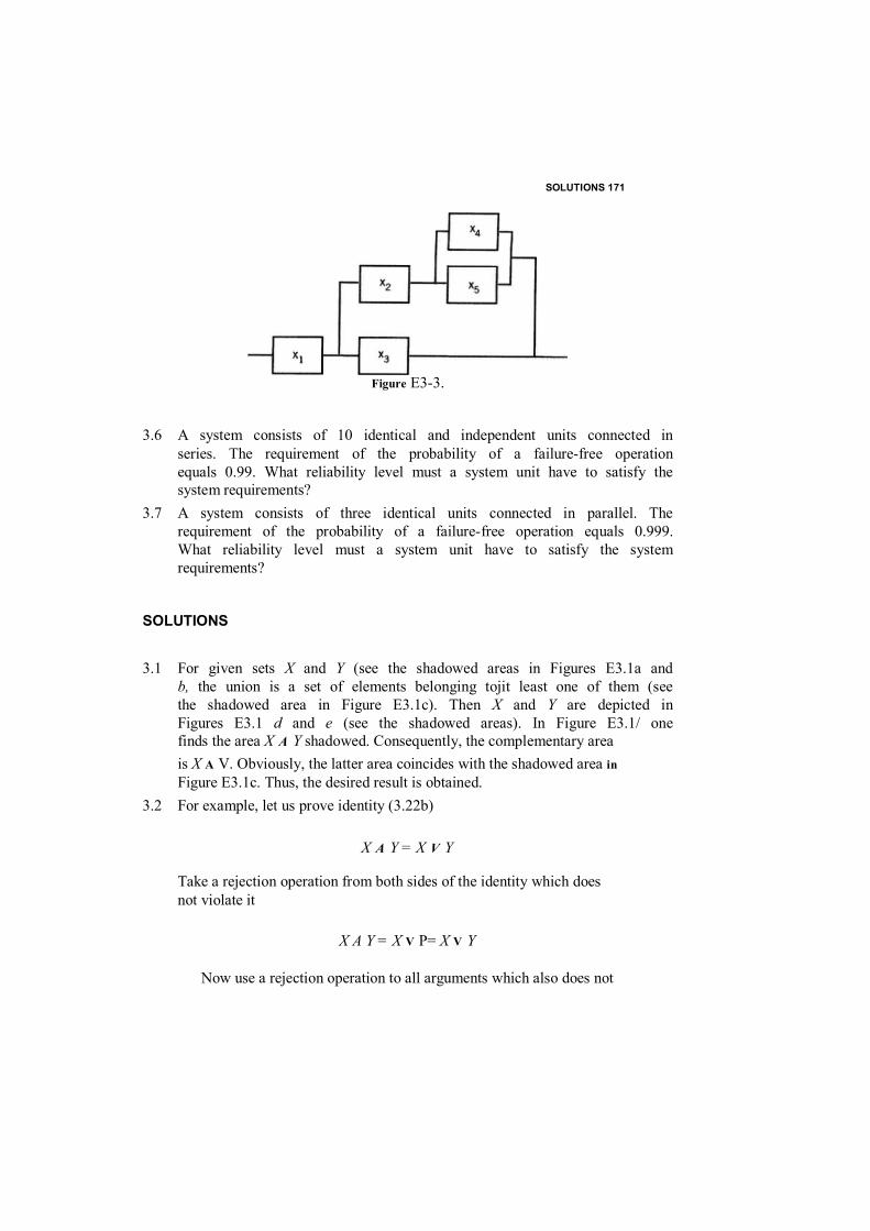
SOLUTIONS 171
3.6 A system consists of 10 identical and independent units connected in series. The requirement of the probability of a failure-free operation equals 0.99. What reliability level must a system unit have to satisfy the system requirements?
3.7 A system consists of three identical units connected in parallel. The requirement of the probability of a failure-free operation equals 0.999. What reliability level must a system unit have to satisfy the system requirements?
SOLUTIONS
3.1 For given sets X and Y (see the shadowed areas in Figures E3.1a and b, the union is a set of elements belonging tojit least one of them (see the shadowed area in Figure E3.1c). Then X and Y are depicted in Figures E3.1 d and e (see the shadowed areas). In Figure E3.1/ one finds the area X A Y shadowed. Consequently, the complementary area is X A V. Obviously, the latter area coincides with the shadowed area in Figure E3.1c. Thus, the desired result is obtained.
3.2 For example, let us prove identity (3.22b)
X A Y = X V Y
Take a rejection operation from both sides of the identity which does not violate it
X A Y = X V P= X V Y
Now use a rejection operation to all arguments which also does not
Figure E3-3.

11 6 UNREPAIRABLE SYSTEMS
violate the identity
X A Y = * X v Y = X v Y
Thus, this identity is reduced to the first one, (3.22a), which was proven in the previous exercise.
3.3 Using (3.22a), one has for the three arguments
X x V X 2 V X 3 = (X , V X 2 ) V X 3 = ( X ] V X 2 ) A X 3
Using the identity X x V X 2 = X y A X 2
one finally obtains
V X 2 v X 3 = X x A X 2 A A"3
Now if for rc — 1 arguments we have
U x i = 0
(a) (b)
(c)

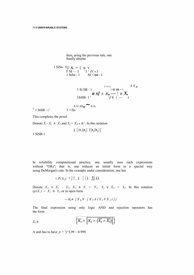
11 6 UNREPAIRABLE SYSTEMS
then, using the previous rule, one finally obtains
U X, = ( u v F M — 1 ' I ^ iV « I ' 1 SiSn - 1 M <iSB - I
u x] A xn — | n X, 1SiSB- 1 ' \J S i — t
n x\ ax„~ n xt
V 1 SiSB - i ' 1 </Sn
This completes the proof.
Denote Yl - X} A X2 and Y2 = XA v A^. In this notation
A [ <* ,A * 2) V(* 4 V* 5)J 1 SiSB-1
In reliability computational practice, one usually uses such expressions without "ORs"; that is, one reduces an initial form in a special way using DeMorgan's rule. In the example under consideration, one has
<P(X () = J f , A [ ( A JT2) A A
Denote X4 V X s - Y l t X2 A Y t = Y2 , Y2 V X3 = Y4. In this notation tpiX,) = X { A Y4 or in open form
— Xj A { X 3 V [ X 2 A ( X 4 V X 5 ) ] j
The final expression using only logic AND and rejection operators has the form
Xx A
A unit has to have p = ]y^L99 ~ 0.999.
1 SiSn- 1
A X , n
1 Si SB - 1 J SI SB - 1
1 <i<.n

Let an unknown probability of failure of a unit be denoted by q . For the system under consideration, one can write
1 - 0.999 = q3
Thus, q = kt.OOl = 0.1, that is, p = 0.9.
11 6 UNREPAIRABLE SYSTEMS
CHAPTER 4
LOAD - STRENGTH RELIABILITY MODELS
For many reliability engineering applications, one needs to investigate the ability of a structure or a piece of equipment to survive under extreme conditions. For a mechanical construction, one speaks of the probability that it can withstand a specified external load (a shock, vibration, etc.) or internal tension. For electronic equipment, one is concerned with the probability that it is able to withstand a specified voltage jump in its power supply or a significant change in its input signals. Both an external load and a construction strength might be considered as random. The first is random in a very natural way, as it depends on environmental factors. The second is random because of the inherent insta- bility of any technological process.
4.1 STATIC RELIABILITY PROBLEMS OF "LOAD - STRENGTH" TYPE
4.1.1 General Expressions Generally, the construction strength X and the applied load Y are random. The problem is to find R, the probability of the system's successful operation, that is, the probability that the applied load does not exceed the actual level of construction strength:
= Pr{X> r} (4.1) 167
Probabilistic Reliability Engineering. Boris Gnedenko and Igor Ushakov

168 LOAD - STRENGTH RELIABILITY MODELS Let Pr{A' < j r } = Fix) and Pr{y < x) = G(jc). Then the probability of a successful operation of the system can be calculated as
R = Pr(* > x) dG(x) = I" ?T( Y < x ) d F ( x ) 00 — 00
= / " [ ! - d G ( x ) = f G ( x ) d F ( x ) (4.2) — CO J —X
If both distributions are continuous, then
/? = / / / (* )<&
where f ( x ) is the density of F(x) and g ( x ) is the density of G(JC). If X and y are considered to be independent r.v.'s, it is convenient to introduce a new random variable, Z = X - Y, with distribution H(x) . Then (4.1) can be rewritten in the form
R = Pr(Z > 0) = rdH(x)dx
4.1.2 Several Particular Cases
Fix) and G(x) Are Normal In this case
f i x ) = _l=e-<*-*>W (4.4) oyv^fl-
where S and crf are, respectively, the mean and the standard deviation of the strength's distribution Fi t) , and
g i x ) = (4.5)
where L and CRG are, respectively, the mean and the standard deviation of the load's distribution Gi t) . Notice that we consider the area of domain of both distributions to range from -oo to Of course, one should consider truncated distributions such that their r.v.'s cannot be negative. But, in practice, S > 3af and L > 3crg, so that such a truncation does not lead to any crucial numerical errors.
dx f ( x ) d x
(4.3)
STATIC RELIABILITY PROBLEMS OF "LOAD - STRENGTH" TYPE 169
Now introduce the new r.v., Z = X - Y . The mean of this new r.v. equals E{Z} = S - L and
<rh - i/tf +
which immediately gives the required result
R = Pr(Z > 0) = f —j^exp •'o ( r h v 2 v
(4.6)
Numerical results can he found from a standard table of the normal distribu- tion.
From (4,6) one can see that the reliability of the construction decreases if the variances of X and/or V increase. Roughly speaking, the more uncer- tain the conditions of use and the more unstable the quality of the construc- tion, the lower is the reliability of the construction.
Example 4.1 The span of a bridge has a safety coefficient c s equal to 5. The safety coefficients is determined as c s = S / L . The coefficient of variation of the strength K s equals 0.05 and that of the land K , equals 0,2. (a) What is the probability of a successful operation of the construction? (b) What is the probability of a successful operation of the construction if the coefficient of variation of the strength is twice as large?
Solution, (a) Assume that L = 1. (By an appropriate normalizing this is always possible.) Then, taking into account the value cs, we obtain S = 5. By definition, the coefficient of variation of the r.v. Z is the ratio Var{Z}/E{Z}2. Therefore, <rg = 0.2 and ay = (0.05X25) = 1.25. The probability of a success- ful operation equals
of 7 5 = j = of — ) = $(3.33) = 0.999517 \ v 1-25 + 0.2 J \ 1.2 ) v 7
(b) In this case the value of the variance is 2.50 and the probability of a successful operation equals
I ( x - E{Z}) S — L
d x = < f >L A22cr,
170 LOAD - STRENGTH RELIABILITY MODELS
F(x) and G(x) Are Exponential In this case
(4.7)
where S is the main strength, and
1
g(x) « - e
where L is the mean load. Using (4.2), we obtain
j 1 S R = j*-~e-x/Le-x/s dx = — r < s x p [ - ( l / L + \ / S ) x ] d x = ----------- ---- ----- (4.9)
'o L L. 'o S + L
In this case the variances do not influence the resulting probability. Of course, it should be mentioned that exponential distributions in problems such as this are very seldom encountered in practice (especially for a distribution of strength). One can find an example of this in Exercise 4,2.
F(x) Is Normal and G(x) Is Exponential Let us use the expression (4.8)
R = f f ( x ) f g ( y ) d y d x
Jo I/O
Notice that
f X g ( y ) d y = f X \ e ~ A y d y = l - e
Therefore, we can write
1 o
o-fi/2-rr
exp
exp
I — exp
I I x - S
K)* = / •'ii
d x
rr;V2-rr h )
1 cxp(~l)pr~ ( exP a,\l7T J0
d x
Combine the powers of the exponential functions of the second terms to get

STATIC RELIABILITY PROBLEMS OF "LOAD - STRENGTH" TYPE 171
f J n

172 LOAD - STRENGTH RELIABILITY MODELS
the complete square form and the free term:
Then
( J f \ ! 2 I T
(Ti * -
s + t + 2 S T " 7F
V 2 l T J [ - S - ( r f / L ) \ /O f
( x - S x
T i L L x - S + + 2 S ~ ~ -
Lj 2 af
a i<Ted x
2 o f
STATIC RELIABILITY PROBLEMS OF "LOAD - STRENGTH" TYPE 173
Change the variables as
t = — - 5 + Aoy2) and <rf dt = dx
Now the final expression becomes
_ } _ < ! > - - - - - _ exp Notice that for most practical problems such as this, the strength S should
be located "far" from the point 0. This means that the value S / L 1 . Incidentally, this corresponds well to the assumption that we do not take into account the truncation of the normal distribution in / = 0. In this case, of
course,
R = 1 - exp
" i >s ~ t(4.10)
l - d>2 l L L 2
o>
1 - <t>(4.11)2 r t L 2

174 LOAD - STRENGTH RELIABILITY MODELS
2 12L L2
Therefore, if one takes into account that the mean load equals L = 1/A, (4.12) can be rewritten as
R ~ 1 - exp| — S A + ^(Aoy)2J
F(x) Is Normal and G(x) Is Biased Exponential The biased exponential distribution with parameter A = 1/L and bias I* is presented in Figure 4.1. In this case
R - f - J0 cr,
where
. 0 for x I *
(X) \ 1 — e ~ M x ~ ' * ) for x > l *
After changing variables, (4.14) becomes
[l - e ~ A x ] d x (4.15)
(4.12)R « 1 — expIf, in addition, Aoy is small, say of order 1, then it is possible to write thenext approximation
(4.13)
1 l x - S 1
G * ( x ) d x exp 42K 2 I (Tf
(4.14)
1 f x - ( S - I * )2 expyi/lTTJ yI* cr,
Omitting the transformations which are quite similar to the above, we
Figure 4.1. Sample of a biased exponential distribution.

STATIC RELIABILITY PROBLEMS OF "LOAD - STRENGTH" TYPE 175
present the final result
/ S - I * \
R = 1 - 4> ----------------- ---- exp
(5 - /*) - A<rf
1 - <t> -
In this case the similar approximate expressions become
--[2(S-f*)A+A2ff/]
(4.17)
for (S - l * ) / a f » 1 and
--[2(S-/*)A+AV/]
for small values of Aoy.
F(x) Is Biased Exponential and G(x) Is Normal Consider the biased distribution of the strength. We do this because it is unreasonable to consider any construction with a strength equal to 0. By assumption, the strength might not be less than s*, so in this case
R - T g ( x ) r f ( y ) d y d x = f g ( x ) d x + f g ( x ) f f ( ( y ) d y y0 / x z s * J 0 V J x
Notice that we again use the lower limit of 0 in the integral. As we pointed out above, for numerical calculations the truncation of the normal distribu- tion at f = 0 to the left can be neglected. A simple transformation leads to
R - f d G ( x ) + r t p ( x ) e ~ l x - ^ d x J - v > JS *
s * - L -I- ( < p (x + s * ) e ~ * x d x
_-[2(S-/*)A+AV/]
(4,16)X
(5 - /*) - Aoy?
1 - <J> R = 1 - exp
(4.18)R = I — exp
d x
(4.19
)
(4.20)

176 LOAD - STRENGTH RELIABILITY MODELS
j f \
174 LOAD - STRENGTH RELIABILITY MODELS
or, in detailed form, e-^dx (4.21)
Avoiding repetition of the transformation which completely coincide with those above, we write the final result directly as
' s* - L + na*
Additional results for some other important particular cases can be found
in Kapur and Lamberson(1977), We would like to mention that this reference contains useful formulas for the Weibull-Gnedenko distribution which is important for description of the strength of mechanical construction.
4.1.3 Numerical Method In general, it is reasonable to use an approximate numerical method. This method is good for calculations using histograms as well as standard statisti- cal tables. In the first case, the approximation is defined by restricted statistical data and their inevitably discrete nature. In the second case, the approximate nature of the solution is explained by a discrete representation of continuous distributions. Because of the approximate nature of these calculations, it is sometimes reasonable to consider the upper and lower bounds of the calculated values.
First, assume that a set of statistical input data is given. The set of observed values of the material strength is X u . . . , X „ and the set of observed values of the load is Yj,.,., Ym. Arrange the ordered set < • ■ ■ < Wn+m where each Ws is one of the .Y/S or one of the 1^'s.
s * - L 1/ - Ja cr.
R = <P|
exp
y/l^ I d }
' s * - L
R „ $
-(s* - L ) n + <P (4.22) + exp

178 LOAD - STRENGTH RELIABILITY MODELS
For each Ws = X, calculate the number of Wr's where Wr = YJ and r < s. Denote this value by k s . This value means that, on the average, in k s cases of m possible observations of the r.v. Y , the load will be smaller than the given strength X . In other words, we might say that with conditional probability ks/m, the investigated system with fixed strength X, will operate successfully if the load will take on one of the possible values of Y . Thus, the complete probability of success is
Obviously, the same numerical result can be obtained if we consider W s = Y j and calculate the number of W ' s where W r = X L for each W s = Y j , r < s . Denote this value by k * . This value means that in k * cases of m
STATIC RELIABILITY PROBLEMS OF "LOAD - STRENGTH" TYPE 179
possible observations of the r.v. X , the strength will be smaller than the specified load Y. It means that with conditional probability k * / m , the investigated system will fail under the load Y; that is, the complete probabil- ity of success is
R - 1 - - Z k t m
Example 4.2 The following data are available: X x m 98.1, X 2 = 98.2, X 3 = 99.4, X 4 = 100.3, X 5 = 101.2, X 6 = 103.5, X 7 = 103.9, X 8 - 104.1,...,
X ] 6 = 110.2; Y, = 79.1, Y2 = 82.4 ................ Ylf! = 98.0, Yiy = 98.3, Ym = 98.5, Y 2 l = 99.5. Calculate the probability that the construction will operate suc- cessfully.
Solution. We find from the data that ki = 18/21, k2 = 18/21, k3 - 20/21, k 4 — • • • — k 15=1. Thus, the result taken by the first expression is
18 18 20 21 + 21 + 21 + 13
From the same data, one finds that k* = • • • = k*8 - 2/16, k ?] — 3/16. Using the second expression, one has the following result:
If tables of the distributions F(x) and G(JC) are available, the numerical calculation of the index R can be performed using the following formulas:
[G((m + 1)A) - G(mA)] (4.23)
R = Z G ( { m + TU)[^((IFI + - F(mA)] (4.24)
1 sm<.M U 2/ /
where A is the chosen increment and M is the number of increments. it is clear that the summation can only be performed in the area of the distribution's domain where the corresponding values of the product terms are significant. For practical purposes, the increments may be chosen to have a value ranging from 0.5 to 0.05 of the smallest standard deviations of the distributions F ( x ) and G(JC). Obviously, the more accurate the result that is
1 329 336
» 0.9792
k n 0, k ~ 2/16, &20 —
1 2 2 3 — + — + — 16 16 16 1 -------- « 0.9792
336
R - Z
1 SM SM
\ - F \ \ m +

180 LOAD - STRENGTH RELIABILITY MODELS
needed, the smaller the increments must be. For practical calculations, the left bound m of the summation must begin with the value k = { m : F( - m A ) < e} where e is chosen in correspondence with the needed accuracy.

STATIC RELIABILITY PROBLEMS OF "LOAD - STRENGTH" TYPE 181
Example 4.3 The strength has a normal distribution with S = 10 and arf = 1, and the load also has a normal distribution with L = 5 and crg = 2 (all values are measured in some conditional scales). Calculate the probability of success R using a standard table of the normal distribution.
Solution. We present Figure 4,2 to illustrate the solution. This figure helps us to see that, for example, the point 7 corresponds to L + cr, and, at the
same time, corresponds to S — 3oy, and the point 9 corresponds to L + 2<rK and to S - oy, and so on. Use a standard table of the normal distribution
and arrange (only for illustrative purposes) the new Table 4.1 with the input data for numerical calculation. Thus, the probability of failure equals 0.98385. A calculation with the use of the strong formula gives
TABLE 4.1 Value of Argument Value of Intermediate
G ( k + 1) - G ( k ) k + 1/2 F ( k + 1/2)
5 6 7 1 = 5
8 9 10 S= 1 0
Figure 4.2. Explanation of the solution of Example 4,3.
A m
Interval [ k , k + 1]
[7,8] t8,9] [9,10] [10,11]
0.00621 0.0668 0.692 0.308
0.00057 0.00295 0.01114 0.00149
0.0920 0.0441 0.0164 0.0049
7.5 8.5 9.5 10.5

182 LOAD - STRENGTH RELIABILITY MODELS
0.01615
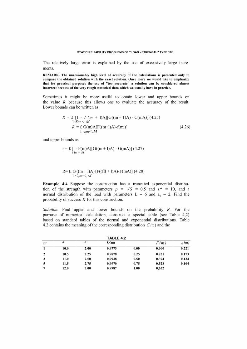
STATIC RELIABILITY PROBLEMS OF "LOAD - STRENGTH" TYPE 183
The relatively large error is explained by the use of excessively large incre- ments. REMARK. The unreasonably high level of accuracy of the calculations is presented only to compare the obtained solution with the exact solution. Once more we would like to emphasize that for practical purposes the use of "too accurate" a solution can be considered almost incorrect because of the very rough statistical data which we usually have in practice.
Sometimes it might be more useful to obtain lower and upper bounds on the value R because this allows one to evaluate the accuracy of the result. Lower bounds can be written as
R - £ [1 - F( m + l)A][G((m + 1)A) - G(mA)] (4.25) 1 £m <,M R = £ G(m)A[F((m+l)A)-f(mi)] (4.26)
I -zm<.M
and upper bounds as
r = £ [l - F(m)A][G((m + I)A) - G(mA)] (4.27) 1 im < M
R= E G{(m + l)A){F((ffl + l)A)-F(mA)] (4.28) 1 <,m <,M
Example 4.4 Suppose the construction has a truncated exponential distribu- tion of the strength with parameters p = \ / S = 0.5 and s * = 10, and a normal distribution of the load with parameters L = 6 and ag = 2. Find the probability of success R for this construction.
Solution. Find upper and lower bounds on the probability R. For the purpose of numerical calculation, construct a special table (see Table 4,2) based on standard tables of the normal and exponential distributions. Table 4.2 contains the meaning of the corresponding distribution G i x ) and the
TABLE 4.2 m X Z | O(m) Fi m ) Aim) 1 10.0 2.00 0.9773 0.00 0.000 0.221 2 10.5 2.25 0.9878 0.25 0.221 0.173 3 11.0 2.50 0.9938 0.50 0.394 0.134 5 11.5 2,75 0.9970 0.75 0.528 0.104 7 12.0 3.00 0.9987 1.00 0,632
184 LOAD - STRENGTH RELIABILITY MODELS
increments of F i x ) in the area of interest. The calculation of lower and upper bounds is performed using formulas (4.26) and (4.28).
In Table 4.2, m is the number of the term in the sum, x is the absolute value, z t is the argument of the standard normal distribution, and z 2 is the argument of the standard exponential function A*(m) = A i m + I) - A(m). Using (4.26), we obtain
R = (0.9773)(0.221) + (0.9878) (0.173) + (0.9938)(0.134) + (0,9970)(0.104) + r = 0.9917
where r is the probability of the "tail" of the strength's distribution with an insignificant influence of the load (all this area must be considered as the area of the "practically absolute" reliability). Using (4.28), we obtain
R = (0.09878)(0.221) + (0.9938)(0.173) + (0.9970)(0.134) + (0.9987)(0.104) + r = 0.9956
The difference between the two values is significant—about 100%. (Notice that if the probabilities are close to 1, one should consider the complemen- tary probabilities, i.e., 0.0083 and 0.0044 in the investigated case.) This means that the values of A are chosen too large.
4.2 MODELS OF CYCLE LOADING
The static models of the "strength-load" type which we considered in the previous section may be referred to as one-cycle loading models. Moreover, this single cycle is assumed to be short enough (but not a shock!), so the strength of the material is assumed to be constant in time. In other words, there is no time for any deterioration or fatigue effects to appear. For practical tasks, such a consideration is important even if the cycles are considered to be independent and identical. Anyway, this more accurately reflects the physical process than a totally static situation. A consideration of the cycle loading is supported by the results of the previous section: the probability determined there is considered as a characteristic of the ability of the chosen construction to withstand a specified fixed load during one cycle.

MODELS OF CYCLE LOADING 185
In real life, the strength of a mechanical construct might monotonically change in time, due to deterioration, fatigue and aging processes, environ- mental influences and so on. (For electronic equipment, the "strength" can fluctuate: the actual tolerance limits can change in time depending on the temperature, humidity, and other environmental influences. Below we often refer to mechanical systems.) The load can also change in time for various obvious reasons. We consider only a simple case: a sequence of shock-type (practically instantaneous) loading. Notice that an investigation of continuous
186 LOAD - STRENGTH RELIABILITY MODELS
loading with a simultaneous changing of the load and strength is a very sophisticated physical problem which an only be solved for some particular cases. We will discuss a very particular case of cycle loading when the strength X and the load V are independent random variables with known distributions Fix) and G ( x ) , respectively. For compactness, the mean value of the strength E(JO will be denoted by S and the mean value of the load E{Y} by L . The strength is assumed to be fixed (known or unknown) or monotonically changing and the load can be represented by a sequence of independent r.v.'s from cycle to cycle.
4.2.1 Fixed Level of Strength Known Fixed Level Suppose that the level of strength is known and equals some value s°, while the load is random with distribution function G i x ) . The values of the load at each cycle are mutually independent r.v.'s. Denote the random number of failure-free cycles by v . The probability that exactly k cycles will be successful equals Pr{i> = /c|s0} = p k q ; that is, the r.v. v has a geometrical d.f. with p = G(s°) and q = 1 - p . The probability of success during K or more cycles equals
Pr{^ > K \ s „ ) = p K where p = Pr{Y £ 5°} = G($°)
The mean number of cycles before failure equals EM = \ / q . If q •«: 1, an approximation in exponential form can be written as
Pr{n S K \ s 0 } = e ~ « K
Unknown Fixed Level Now assume that is unknown but constant during the total period of the system's operation. The only thing we know is the prior distribution Fix). In this case
Pr { u ^ K } = / [ G ( x ) ] K d F( x ) J c
where C is the domain of the distribution F i x ) . Let the probability q i x ) = 1 — G(JC) be small "on average." In practice, this corresponds to the condition
where a s is the standard deviation of the d.f. F i x ) . We can conclude that the
S - L

DYNAMIC MODELS OF "STRENGTH - LOAD" TYPE 187
right "tail" of the distribution G(JC) is concave in the essential area of the domain of the distribution F(JC). Then the following simple bound is true:
Pr{f > A:} < [G(S)]*
The mean number of cycles is
E H = / [ 1 ~G(*)]-'c/F(x) J c
The corresponding approximation for small q is
E H < [ 1 - G ( S ) ] - 1
4.2.2 Deteriorating Strength If the expected number of successful cycles is very large, that is, the operational time is sufficiently large, we might assume that the level of the system's strength decreases in time. Indeed, most materials deteriorate with time and, consequently, the system strength becomes weaker and weaker. We will consider several simple models.
1. Assume that the material strength decreases from cycle to cycle in such a way that pk + i = apk where pk is the probability of success at the fcth cycle and a is constant, 0 < a < I. Then
Pr { i / a K \ s ° , a } = p ( p a ) ( p a z ) ■ ■ ■ { P < * K ~ l )
= pK Ft ak=pKa(K^2/2
and the mean number of successful cycles is EH = £ pV*-'^
2. Again consider the case where the level of the strength is known and the deterioration is described by an exponential decrease of this level: at the fcth cycle, the level of the strength is xk = s°ak where 0 < a < 1. The probability of success over at least K cycles equals
Pr{*> > X*|s°, a} = n G(s°a*)
Note that G(J°A*) > and for the most commonly used distributions, this discrete function is concave. Then
Pr{y > K|s0,a} < G(sV*/2>)

188 LOAD - STRENGTH RELIABILITY MODELS
The mean number of cycles until the system fails equals
W = lpj + 2 p(p2 + 3 p t p 2 p 3 + = p,(l + p2(l + p3( 1 + • ■ ■ ) ) )
3. For a known distribution F(*) of the initial value of the strength, the probability of success equals
Pr{* £ K \ F{ x ) , a ) - / f l G ( a k ) d F( x ) J C is k ^ K
We do not have a simple approximation for this case,
4.3 DYNAMIC MODELS OF "STRENGTH - LOAD" TYPE
In the previous sections we considered a simple version of the dynamic loading process, that is, the cycling process. That scheme is sufficiently good to describe some specific mechanical systems. But for most electronic systems the process of "loading" should be described as a continuous stochastic process. Indeed, in this case one considers a process of randomly changing the system parameters inside the tolerance zone. We will consider only a simple case where one-dimensional stochastic process crosses a specified level.
4.3.1 General Case Consider a differentiate stochastic process x { t ) . We are interested in the distribution of intervals between neighboring intersections of a specified level a by the process. At first, we find the probability that the process will intersect the level a at moment t . This event happens if the two following events have occurred:
{ * ( / ) < a } and {*(( + d t ) > a }
In other words, the probability of the event equals
Pr{(jt(r) < + d t ) > a)}
(4.29) Let v ( t ) be the speed of the process, that is, v ( t ) = d x ( t ) / d t . Now we can rewrite (4.29) in the new form
Pr{fl - v ( t ) d t < x ( t ) < a } (4.30)
To find this probability, we need to know the density function of the joint distribution f i x , t>|/) of the ordinate x of the process x ( t ) and its derivative for the same moment of time t . Using these terms, we can write
Pr{a - l>(() d t <x(f) <«)- f ^ f f ( x , v \ t ) d x d t (4.31) J 0 a — v d t
DYNAMIC MODELS OF "STRENGTH - LOAD" TYPE 189
The internal integral can be computed instantly because of its special limits
/ a f ( x , v \ t ) d x = d t v f ( a , v \ t )
< j ~v d i
Substitution of (4.32) into (4.31) gives us
Pr{« - v ( t ) d t < x ( t ) a ) = d t C f ( a , v \ t ) v d v (4.33) J o
This formula shows that the probability of the intersection of the specified level by the stochastic process during the infinitesimally small time interval d t is proportional to the length of the interval. This allows one to introduce the time density for this probability p ( a \ t ) . Using (4.33) gives
Pr{a - u ( t ) d t < x(f) < a} = p ( a \ t ) d t (4.34)
and, consequently,
p ( a \ t ) m r f ( a , u \ t ) v d v (4.35) ■'o
Analogously, one can find the derivative of the probability p ( a \ t ) :
d , - ~ p ( a \ t ) - - j f ( a , v \ t ) v d v
(4.36)
Adding and subtracting (4.35) and (4.36), one can easily obtain the two following equations:
p ( a \ t ) + — p ( a \ t ) = f ( a , u \ t ) \ v \ d u (4.37) d t J — o a
and
p ( a \ t ) - ~ p { a \ t ) = f ( a , v \ t ) v d v (4.38) d t ^ — o o
It is clear that
f ( a , v \ t ) - f ( v \ a , t ) f ( a \ t )
Then one can rewrite (4.37) and (4.38)
p ( a \ t ) + j [ P { a \ t ) -./(«|r>E( |^r)||Jf( f ) = a ) (4.39)
p ( a \ t ) - ~ p { a \ t ) ~ f ( a \ t ) E { V ( T) \ X ( t ) = a } (4.40)

190 LOAD - STRENGTH RELIABILITY MODELS
Using (4.35) for any time interval T , one can obtain the mean time of x ( t ) being over the specified level a . To obtain the result, we use the following simple arguments. Let us divide the total period T into n small nonoverlap- ping intervals located around the points t j , ) < j < n . For some t j , we can write
Pr{A-(fy) > a} = rf(x\tj)dx (4.41) a
Assume that the intervals S / s are chosen so small that changing signs by the function x(t) - a can be neglected. Next, introduce the indicator func- tion { d t j } + such that
IS, if *(0 - a > 0 , tj= ' Y (4.42)
\ 0 otherwise
Using this notation, one can write that the total time for which the function jv(f) exceeds the level a equals
Ta~ L A, (4.43) 1 <,i<,n
and the mean time when the function jt(r) exceeds the level a equals
E{rfl}= L E{A,} (4.44)
1 S.j £ n
At the same time,
E{A,)-a, f f ( x \ t j ) d x (4.45) a
Using (4.45) and taking the limit in (4.44), we obtain the expression for the total time for which the process ;c(r) exceeds the level a :
E{Ta} = rrf(x\t)dxdt (4.46) J a
If one is interested in the average number of intersections na during a time interval T , the same simple arguments can be used. Now introduce another
indicator function
1 if JT( r) — a > 0 in the interval at least once 10 otherwise N , =

DYNAMIC MODELS OF "STRENGTH - LOAD" TYPE 191
The total number of intersections during period T equals
K = Z N j I s/sn
Again the mean value can be expressed as
E(Nfl)= £ E{Wy} (4.47) 1
where
E { N j ) ~ p ( a \ t J ) 8 J
(4.4
8)
Taking the limit of (4.48) with the substitution of (4.35), we obtain E { A U - [ T r v f ( a , v \ t ) d v d t (4.49)
-'o -'o
In addition to (4.46), the last expression permits us to write the expression for the mean time t a for which the process x ( t ) exceeds the level a during a single intersection. Indeed,
* BJAU <4'50)
or, using the corresponding complete expressions,
f T f f ( x \ t ) d t ta = - J o J a ------------------ (4 51) a j oo \ '
/ / u f ( a , u \ t ) d v d t yo o

192 LOAD - STRENGTH RELIABILITY MODELS
All of these results are essentially useful for stationary processes because in this case all of the functions do not depend on the current time, that is, f ( x \ t ) = f i x ) and f ( x , v \ t ) = f { x , u ) . Then all of the previous results can be
DYNAMIC MODELS OF "STRENGTH - LOAD" TYPE 193
rewritten in the simpler form, namely,
E { r f l } = T f ° ° f ( x ) d x
a
E TO = T[ ° ° u f ( a , v ) d v
f f ( x ) d x . a
Tl v f ( a , v ) d v o
Naturally, for the stationary process the values of E{TJ and E{/V„} depend
only on the length of the period T . More precisely, they are proportional to T . The mean time E{fa} for which the process exceeds the level a does not depend on T . For a stationary process one can also introduce the mean number of itersections per unit of time Aa:
(4.55)
that is, the probability of a level crossing in a unit of time.
4.3.2 Gaussian Stochastic Process To calculate all of the above-mentioned parameters of the specified level intersection, one needs to know the characteristics of the stochastic processes f ( x \ t ) and f ( x , v \ t ) . For stationary processes, one needs to know f i x ) and f i x , v ) . Fortunately, for the most important practical case—the Gaussian stochastic process (GSP)—sufficiently simple formulas can be obtained.
Note that the Gaussian process is often taken as the mathematical model of the random change of electrical parameters over time. There are many physical reasons to use this model because the influence of the number of internal and external factors leads to the formation of conditions for the validity of such a model. Indeed, these various factors might often be considered as relatively independent, and the influence of each of them on the resulting process is relatively small. Of course, the correctness of these hypotheses should be checked or verified each time.
We consider only a stationary process for which we know the mean E{X} and the variance crj. For a normal process in a stationary regime, the ordinate distribution is
(4.52)
(4.53)
(4.54)
where = K x i 0) and K x i r ) is itself the correlation function.

194 LOAD - STRENGTH RELIABILITY MODELS

DYNAMIC MODELS OF "STRENGTH - LOAD" TYPE 195
It is known from the theory of stochastic processes that the ordinate of the GSP and its derivative for the same moment of time are noncorrelated. Thus, the joint density function can be presented as the product of the two separated densities
f ( x , v ) - R x ) f ( v )
or
( x ~ E { X ) ) 8
2 a2
8 a ?
(4.56)
- V2
f ( x , v ) = 2r2 . <«*) exp exp
196 LOAD - STRENGTH RELIABILITY MODELS
Note that the variance cr3 can be expressed through the correlation function of the process as
(4.58) T-0
and v(t) equals 0 because the stationary process is considered. An expression for Aa can be obtained from (4.55) after the substitution of (4.57)
( a - E{A"})
The expression for E{ra} can be obtained in an analogous way:
a — xr = t t — exp
where <f>(.t) is the normal distribution function.
4.3.3 Poisson Approximation The crossing of a "high level" threshold by a stochastic process is of great interest for reliability analysis. It is clear that the probability of the crossing in this case should be sufficiently small; that is, such intersections are "rare events." As we mentioned above, the sequence of rare events forms a Poisson stochastic process. We omit the proof of the fact that in this particular case this hypothesis is also valid. Here we accept this as a known fact.
In general, we may assume that the mean number of intersections E{Na) of level a for a specified period T approximately equals the mean number of events AT for some Poisson process with parameter A. Thus, this parameter
Ty —
c r u (4.59) = P ( a ) = exp
'.7T(T,.
(4.60)1 - <t>
2 7Tu}
DYNAMIC MODELS OF "STRENGTH - LOAD" TYPE 197
A ------- (4.61)
where E[ N J is determined by (4.51) or (4.55), depending on the type of stochastic process under consideration.
We will not write the expressions for the Poisson probabilities. The reader can do it easily him/herself. We only write the expressions for the probabil- ity of a failure-free operation (i.e., no intersection during the time T) for the nonstationary and stationary cases using the corresponding values of E { N a ) . For the nonstationary process one has
- f T Tv f ( a , v \ t ) d t Jn Jc\
'0 J o
and for the stationary process one has
Tf v f ( a , v ) d t J o
For Gaussian processes, the probability P 0 ( T ) can easily be written with the use of A0 from (4.59).
It is difficult to estimate the error obtained via the use of such an approximation for the Gaussian process. The only simple physical explana- tion lies in he fact that there is practically no correlation between neighbor- ing moments of intersections of the specified "high level." (To check this fact, one should take into consideration the mean time between two neigh- boring intersections: "too much water has passed under the bridge" after the previous intersection!)
Example 4.5 Consider equipment characterized by a two-dimensional pa- rameter with components X and Y . Both components X and Y are fluctuat- ing in time. Their fluctuations are described as the identical independent stationary Gaussian processes with means equal to 0 and correlation func- tions
K x { t ) = K y ( r ) = <r2e-°|r'|cos /3|r| + ^ sin /3|r|j (4.64)
The tolerance limit area of the equipment parameter is represented by a sphere with radius a. Find the mean time that the system's parameter is spending inside the tolerance limit area if, at the moment t = 0, both X ( t ) and Y ( t ) are in the center of the tolerance sphere.
can be easily expressed as
(4.62)Po = CXP
(4.63) P 0 = exp

198 LOAD - STRENGTH RELIABILITY MODELS
Solution. Let
R ( t ) = y / x \ t ) + Y \ t ) (4.65)
and
d R ( t ) = (4-66)
Using (4.56), we can write
f f ( r ) d r T = ---------------------- (4.67)
/ v r f ( a , v r ) d v r J n
where f ( a , v r ) is the joint density of the distribution of the two r.v.'s R and v r for R = a . Consider an arbitrary period of time T . There are, on average, k a T intersections, and the vector parameter represented by the point ( X , Y ) is outside the specified tolerance zone during the mean time E{ra}Aa7\ Conse- quently, the system parameter will be inside the tolerance zone, on average, during the time T [ 1 - E{fa}Aa], The mean time that the parameter spends inside the tolerance zone is
r = 1 Tx al =r-E{U (4.68)
Using (4.56), we can write
f f ( r ) d r J o _________ -oo / v r f { a , v r ) d v r J n
r =
DYNAMIC MODELS OF "STRENGTH - LOAD" TYPE 199
Now we find the corresponding densities and compute the final result in a compact and constructive form. At first, notice that the r.v.'s X and Y are independent and have normal distributions, so
1 2tr
I 2tt<T
( x 2 + y 2 ) f ( * , y ) = (4.69) exp
CONCLUSION 200
Further,
f ( r ) d r - Pr{r < R < r + d r ) = / /
J J
r< if)
n
that is, /(r) is a Rayleigh density. To determine the density f i r , u r ) , we need to consider a system of four normally distributed r.v.'s: X , Y , v x = d X ( t ) / d t , and v y = d Y( t ) / d t . For a Gaussian process, all of these r.v.'s are independent. The variances of v x and
v y are identical and equal = a 2 ( a 2 + p 2 )
Thus, v x and V y do not depend on the coordinates of ( X , Y ) and have a circle normal distribution; that is, the projection of the vector ( v x , u y ) on the direction of R has a normal distribution with variance (4.71). Thus, the
two-dimensional density f ( r , v r ) can be expressed in the following way: f ( r , v r ) = f ( r ) f W = — e x P ~
Xexp
l a 2 { a 2 + p 2 )
After substitution of (4.70) and (4.72) into (4.68), we obtain the final result
a y a + f t ^ ' "2
+ p2 This example shows that the use of stochastic process theory to find reliability indexes is not a simple task. But difficult practical problems always need the use of more or less complicated mathematical tools. Note also that besides the technical complexity of the solution there are also some special needs concerning the input data. Such data are not always available.
f ( x , y ) d x d yx 2 + y 2 < r + d r
1 ,r+dre_r2/2„2rdrd(p _ '-rWdr (4.70)
cr
2Tt(T2 JQ
d 2 K x ( r )
(4.71)d r 1 r = 0
1 2cr2 J y j 2 i T ( T 2 { a 2 + p 2 )

SOLUTIONS 201
CONCLUSION
We presented only a very brief description of the problem which could be explained by our intention to consider, primarily, system reliability. The problem related to the degradation of mechanical constructions under the random load and fluctuation of their physical parameters and the strength

202 LOAD - STRENGTH RELIABILITY MODELS
are special branches of modern reliability theory. Each of these branches must occupy a separate book.
The reader can find some appropriate formulations of the problem of reliability of mechanical systems and many useful related results, for exam- ple, in Kapur and Lamberson (1977). We would also like to mention Bolotin (1975). In Becker and Jensen (1977) one finds an analysis of a similar mathematical problem related to the reliability of electrical equipment under a stochastic fluctuation of parameters. Mechanical problems in reliability engineering are considered in Konyonkov and Ushakov (1975). Some results concerning the reliability of mechanical systems are contained in Ushakov (1985, 1994).
Interesting results concerning accumulations of random shocks can be found in Barlow and Proschan (1975). Elegant mathematical results can be obtained with the use of the Kolmogorov equations if the process of the parameter fluctuation can be described as a Markov process.
One can find a lot of interesting results in the extensive literature on noise analysis in radio equipment. This powerful branch of applications was stimu- lated by the pioneering work of Rice (1944, 1945).
At last, we would like to mention that this problem must be considered on a serious physical level. This chosen mathematical model must correspond to a real object, either electronic equipment or a mechanical construct. Writing a set of abstract models covering this subject area seems to be a hopeless task. Besides, it is not a simple task to find the appropriate statistical data for the models dealing with the random behavior of real parameters.
REFERENCES
Barlow, R. E., and F. Proschan (1975). Statistical Theory of Reliability and Life Testing. New York: Holt, Rinehart, and Winston.
Becker, P. W., and F. Jensen (1977). Design of Systems and Circuits for Maximum Reliability and Maximum Production Yield. New York: McGraw-Hill.
Bolotin, V. V. (1975). Application of Methods of Probability Theory and Reliability Theory for Construction Design (in Russian). Moscow: Stroiizdat.
Gertsbakh, I. B., and Kh. B. Kordonsky (1969). Models of Failure. Berlin: Springer, Kapur, K. C, and L. R. lamberson (1977). Reliability in Engineering Design, New
York: Wiley. Konyonkov, Yu. K., and I. A. Ushakov (1975). Aspects of Electronic Equipment
Reliability Under Mechanical Stress {in Russian). Moscow: Sovictsko Radio. Rice, S. O. (1944, 1945). Mathematical analysis of random noise. Bell Syst. Tech. J.
vot, 23, no. 3, and vol, 24, no. 1. Sveshnikov, A. A. (1968). Applied Methods of the Stochastic Function Theory. Moscow:
Nauka.
SOLUTIONS 203
Ushakov, I. A., ed. 0985). Reliability of Technical Systems: Handbook (in Russian). Moscow: Radio i Sviaz. Ushakov, I. A. (1994). Handbook of Reliability Engineering. New York: Wiley. Vinogradov, O. G. (1991). Introduction to Mechanical Reliability: A Designer's Ap- proach. New York: Hemisphere.
EXERCISES
4.1 The distributions of both a strength and a load are normal. The mean of the load is known: L = 10 conditional units and the standard deviation a g = 2. Find the parameters of the distribution of the strength S and oy which deliver a probability of failure-free operation equal to R = 0.995.
4.2 The distributions of both the strength and the load are exponential with parameters 1/5 and 1/L, respectively. L = 1 conditional unit. Find S which delivers a probability of failure-free operation equal to R = 0.995,
4.3 The strength's distribution is normal with unknown parameters S and oy and a known coefficient of variation k = 0.04. The distribution of the load is exponential with L = 1 conditional unit. Find the parameter S which delivers R = 0.999.
SOLUTIONS
4.1 First of all, notice that the problem as formulated here is incorrect: one should know in advance the mean of the strength a or its standard deviation or the coefficient of variation k = o-*/S2. Without this correction the problem has no unique answer.
Let us assume that one knows 4k — 0.04. The problem can be solved by sequential iterations. For choosing a first value of S , notice that because of the requirement, R = 0.995, there must be at least more than L + 2.5<7-K. Choose S(1) == L + 3ag = 16. Then
<t} = J k ( S ( l ) ) 2 - vT0704)(256y = 3.2
Now it is clear that this level of strength is unacceptable. Choose the next value, for instance,
S(2) = L + 3 o ■ + 3<rr(1> = 26
204 LOAD - STRENGTH RELIABILITY MODELS
This value of S<2) leads to
o)n = k ( S (2>)2 = /(0" 04) (676) « 5.2
Check the above obtained result
26 - 10 I 26 - 10 \
(MT53)_,1,(2'22)°0-987
Thus, the value 5 is still smaller than one needs to deliver R = 0.995. The procedure continues. (We leave it to the reader to obtain the final numerical result.)
4.2 From (4.9) one can write
LR 1 • (0.995) = 199 conditional units I - R
This coefficient of safety is too large. The assumption that both strength and load distributions are exponential is unrealistic in practice. At the least, this is quite unreasonable as a distribution of strength.
4.3 For a highly reliable construction, one can use (4.12) or (4.13). This gives
1 / 2 5 0.0452 \
~ 2 \ T U ~ j
or
0.025
= 0.001
The latter can be rewritten as
0.0252 - 5 = 6.9
We leave to it to the reader to complete the solution.
P = 0
S = 0.005
= 0.999 R = 1 - exp
exp

CHAPTER 5
DISTRIBUTIONS WITH MONOTONE INTENSITY FUNCTIONS
For a quantitative characterization of reliability, we must know the failure distributions. Such detailed and complete information is not always available in engineering practice. Fortunately, in some cases we do not need to know the particular type of distribution, it is enough to know only some parameters of the distribution and the fact that this distribution belongs to some special class of distributions. In this case we can often obtain bounds on the reliability indexes based, for example, on the known mean and variance or other similar parameters of the distribution. Concerning the distributions, we need only know that they belong to the class of distributions with a monotone failure rate. There are several main classes of such distributions and these are described below.
5.1 DESCRIPTION OF THE MONOTONICITY PROPERTY OF THE FAILURE RATE
A very natural phenomenon of reliability as it changes over time is often encountered: the longer an item is functioning, the worse the residual reliability properties become. For many practitioners this phenomenon seems almost to be unique. Indeed, deterioration, fatigue, and other similar physical processes lead to a worsening reliability. Such phenomena (and their associ- ated distributions) are called aging.
Probabilistic Reliability Engineering, Boris Gnedenko and Igor Ushakov
206 DISTRIBUTIONS WITH MONOTONE INTENSITY FUNCTIONSBut there also exists another property: if an item works for a long period of time, we become more sure of its reliability. Sometimes this property follows from a physical phenomenon connected with a change in the chemical and mechanical features of an item: a penetration of one material into another through contacting surfaces, a strengthening of the joining materials, a "self-fitting" of frictional parts, and so forth. Sometimes this is connected with a "burning-out" effect. This phenomenon is called younging. As an example of the latter property, consider a mixture of two equal parts of items: one with a constant M'lTF equal to 100 hours and another with a constant MTTF equal to 900 hours. We observe an item chosen at random from this mixed group of items. At the moment t = 0 the MTTF equals
T - T x p + T 2 ( \ - p ) = 100(0.5) + 900(0.5) = 500 hours
and the probability of a failure-free operation, say during 200 hours, equals
Pr{£ ^ 200[ starting at t = 0} - 0.5 But if it is known that at t = 101 hours the item is still functioning, the values of both reliability indexes under the condition that the new trial starts at f = 101 hours change:
T* - T 2 = 799 hours and Pr{f a 200|starting at t - 101} - 1
Both values for the used item are larger than for the new item on the average. Of course, there is no change in the item itself. We have only new information which allows us to make a posteriori a new conclusion about the item's reliability. An analogous example was considered in Chapter 1 when the mixture of exponential distributions was analyzed.
Notice that we observe a similar effect in "burning-out." It is normal practice to use some stress tests (temperature shocks, accelerated vibration, etc.) for selecting technologically weak items. The same effect is observed when weak units and manufacturing defects are eliminated during a high- failure "infant mortality" period under normal conditions.
It is the appropriate time to recall the ancient Greek myth about the Spartans who killed their weak and ill infants by throwing them from a high rock into a canyon. They did this to ensure that their remaining children would be healthy and strong. (We must state that this is only a myth: it was not a custom in the ancient democracy. As new sources claim, rich, free citizens of Greece replaced their weak and ill infants with the healthy babies of poor families.)

DESCRIPTION OF THE MONOTONICITY PROPERTY OF THE FAILURE RATE 207 Of course, there are no "immortal" items. First of all, if a failure rate decreases in the initial phase, an increase in the failure rate at some point is inevitable. Many items have the failure rate function of a "U-shaped form (see Figure 2,2). Second, even a probability distribution with a decreasing
208 DISTRIBUTIONS WITH MONOTONE INTENSITY FUNCTIONSfailure rate has P ( = 1 - F(<») = 0. (Of course, this puts a special condi- tion on the decreasing failure rate function.) The exponential distribution is the boundary distribution between distributions with increasing and decreas- ing rates. One of the basic characteristics in further analysis is the "conditional instantaneous density" of the time-to-failure distribution. For this conditional density, we usually use the terms failure rate or failure intensity. The strict mathematical definition of this, as we mentioned above, is
A C ) - ^ (5-.)
Thus, in reliability terms, this is the instantaneous failure distribution density at time t under the condition that the item has not failed until t . A better explanation can be presented in terms of an "element of probability." A(OA is the probability of an unrepairable unit failure in the interval of time [ / , t + A] under the condition that the unit has not failed by moment t . This conditional density changes continuously with time. Sometimes it is useful to consider the function:
A(/) = f ' \ ( x ) d x J n
Integration of (5.1) and (5.2) yields
f ' \ ( x ) d x
In this chapter we consider only the simplest properties of distributions with a monotone failure rate. A more detailed analysis of the subject can be found in Barlow and Proschan (1975). We do not consider the U-shaped A(/)'s or the nonmonotonic ones. Notice that a nonmonotonic A(f) is not very unusual at all. The following example from Barlow and Proschan (1975) can be analyzed in very simple terms.
Example 5.1 Consider an unrepaired system consisting of two different units in parallel. Each unit has an exponentially distributed TTF. For this system
P ( t ) = 1 - ( 1 - -
and
A1e~A,f + X 2 e - (A, + A2)e-(A'+A^' = + e A 2 I _ g - ( A ,+ A 2 ) , — (5.4)
(5.2)
= e - M » P ( t ) = exp (5.3)
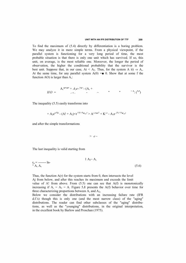
UNIT WITH AN IFR DISTRIBUTION OF TTF 209
To find the maximum of (5.4) directly by differentiation is a boring problem. We may analyze it in more simple terms. From a physical viewpoint, if the parallel system is functioning for a very long period of time, the most probable situation is that there is only one unit which has survived. If so, this unit, on average, is the most reliable one. Moreover, the longer the period of observation, the higher the conditional probability that the survivor is the best unit. Suppose that, in our case, Ai < A2. Thus, for the system A it) -» A,. At the same time, for any parallel system A(0) =■ 0. Show that at some f the function AO) is larger than A,:
A,*"*'' + A2e~x*' - (A, + H O = e - x , , - ~ " " > A: (5'5)
The inequality (5.5) easily transforms into
+ A2e"Aj' - (A! + A2)<r<A|+A*>r > A^"*'1 + K^' - A1e_(A,+A*>'
and after the simple transformations
> e ~
The last inequality is valid starting from
1 A2~ A, rn = ------- ln- ° A, A,
Thus, the function A(r) for the system starts from 0, then intersects the level Aj from below, and after this reaches its maximum and exceeds the limit value of A! from above. From (5.5) one can see that A(f) is monotonically increasing if A, = A2 = A. Figure 5.1 presents the A(f) behavior over time for three characterizing proportions between A, and A2, Below we consider the distributions with an increasing failure rate (IFR d.f.'s) though this is only one (and the most narrow class) of the "aging" distributions. The reader can find other subclasses of the "aging" distribu- tions, as well as the "younging" distributions, in the original interpretation, in the excellent book by Barlow and Proschan (1975).
(5.6)
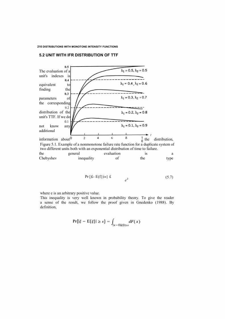
210 DISTRIBUTIONS WITH MONOTONE INTENSITY FUNCTIONS
5.2 UNIT WITH IFR DISTRIBUTION OF TTF
The evaluation of a unit's indexes is
equivalent to finding the
parameters of the corresponding
distribution of the unit's TTF. If we do
not know any additional
information about the distribution,
the general evaluation is a Chebyshev inequality of the type
Pr{|£- E(f}|i«} £
where e is an arbitrary positive value. This inequality is very well known in probability theory. To give the reader a sense of the result, we follow the proof given in Gnedenko (1988). By definition,
0.5
0.4
0.3
0.2
0.1
t 2 4 6 8 1
0 Figure 5.1. Example of a nonmonotone failure rate function for a duplicate system oftwo different units both with an exponential distribution of time to failure.
0
(5.7)2 e

UNIT WITH AN IFR DISTRIBUTION OF TTF 211
Becausc in the domain of integration ( l / e ) \ x — E{£}| > 1,
/ d F ( x ) < \ ( ( x - E { t ) f d F { x )
1 r" , , ,2 Var{^} o-2 O - CC C c
This completes the proof. Inequality (5.7) is universal and so is not too constructive for practical purposes (as with any universal tool). For instance, one sees that (5.7) only makes sense when e > tr. In other words, this estimate is not true in some area around the mean. But notice that, at the same time, at the distribution's tails, the estimate is very rough. Suppose that additional information is available. Then we can obtain narrower bounds. Consider the class of IFR d.f.'s. We first prove several additional statements.
Theorem 5.1 The graph of an IFR d.f. P i t ) crosses the graph of an arbitrary exponential function e ~ A I at most once from above. If these two functions do not cross, P i t ) lies strictly under this exponential d.f. (see Figure 5.2).
Proof. The intensity function A(f) for the IFR distribution might increase infinitely or be bounded above by some number A*. In the first case, there exists a moment tn when
A('o) = /'°A(Jc)<fr-A*c J n
and, for any y ^ r0,
A(y) Ay
Figure 5.2. Explanation of the contents of Theorem 5.1: possible types of relationships between the exponential function and dif- ferent IFR distributions of time to failure.
212 DISTRIBUTIONS WITH MONOTONE INTENSITY FUNCTIONS
(5.8)
In the second case, for any t > 0, we have A(r) s A* and, consequently, A(/) never crosses A t . Thus, for any t ,
P(r) < e"A '
From (5.8) and (5.9) it follows that the "right tail" of the IFR distribution decreases faster than the corresponding tail of the exponential function.
Corollary 5.1 If an IFR d.f. P i t ) has a first derivative different from 0 at
/ = 0, say
then P ( t ) lies everywhere below e at.
Proof. The proof follows from the fact that A(f) > at for all t. Some hint of a graphical explanation can be found in Figure 5.2.
Corollary 5.2 An IFR d.f. P i t ) necessarily crosses e ~ x ' from above once if both distributions have the same MTTF equal to T .
Proof. By Theorem 5.1 both d.f.'s have to intersect once or not intersect at all. The second statement contradicts the corollary, so we need to check this. Suppose that both d.f.'s do not intersect. This means that
which contradicts the statement concerning the equality of the MTTFs. For a graphical explanation, refer to Figure 5.2.
Theorem 5.2 For an IFR d.f. P i t ) , the function
7P( T )
d
— a
(5.9)
because AO) increases. Thus,

UNIT WITH AN IFR DISTRIBUTION OF TTF 213
decreases with increasing t .

214 DISTRIBUTIONS WITH MONOTONE INTENSITY FUNCTIONS
Proof. AO) is convex, so log P i t ) = -A(() is concave. But then
log J^ Q - togP(O) t - 0
decreases with increasing t . Consequently,
1 ^(0 7losm
decreases in t . After substituting P(0) = 1 and using an exponential transfor- mation, the proof of the theorem follows.
This theorem produces the following interesting corollaries.
Corollary 5 3 For an IFR d.f. P i t ) ,
P( x ) < ; [ P i t ) } 1 ' '
for all x > t .
This allows us to predict (i.e., to compute a lower bound) the probability of a failure-free operation of an IFR unit for a specified time, if we know the value of P i t ) for a smaller interval of time. This corollary can be of great use for an application in testing IFR units during a short testing period.
Corollary 5.4 For an IFR d.f. the initial moments of all orders are finite.
Proof. Indeed, for any t,
f ™ x r P( x ) d x < f " x ' { [ P( t ) ] V y d x = f"xre~p* dx < oo
where [P(f)],/" is replaced by The reader knows that the exponential d.f. has the moments of all orders.
The last corollary shows that arguments about the properties of "aging" units, which seem to be just qualitative statements, have led to very strong restrictions on the moments of an IFR d.f. Incidentally, note that the coefficient of variation of the IFR d.f. is always less than 1. Now, using all of the above results, the following important characteristics of IFR d.f.'s can be obtained.

UNIT WITH AN IFR DISTRIBUTION OF TTF 215
Theorem 5.3 If is the quantile of an IFR d.f. P i t ) , PrU > = p , then
a e~a(>> for t <,
< e~a*r for t > ip
ln(l -p) a - - - - - - - - - - -
Proof. An exponential function can be found which goes through the point ( £ p , 1 - p ) . The parameter of the exponent can be found from the equation
e - « f p = i - p
We then use Theorem 5.1 to complete the proof.
Theorem 5.4 A lower bound for an IFR d.f. is determined
by
n o = {e0
where t is the MTTF
r = f p ( t ) d t J o
Proof. We first present a rigorous proof. For an IFR distribution the function A(r) is an increasing convex function, so by Jensen's inequality
E{A(£)} < A(E{£}) — A(T) (5.10)
Denote P i t ) = y and rewrite
E{A(£)} -E{-ln/»(f)} = E{-Iny} - [ \ n y d y ~ 1 (5.11) ■'o
From (5.10) and (5.11)
E{A(f)} = 1 ^ A(T) = -In P i T )
immediately follows where
P { t )
where
,/T for t < T for t > T

216 DISTRIBUTIONS WITH MONOTONE INTENSITY FUNCTIONS
P i T ) > e ~ 1 (5.12)

217 DISTRIBUTIONS WITH MONOTONE INTENSITY FUNCTIONS
0
[ P{ t ) \ W ' > [ P( T ) ] 1 / T > e - V T
and, finally, for t < T the required result is obtained
P ( t ) > e ~ ' / T
The same result can be derived from simple explanations based on a graphical presentation (see Figure 5.3). The first inequality follows immediately from a comparison of the exponen- tial function e ~ ' / T and a degenerate function G ( t ) with the same MTTF
for t t z T for t > T
The degenerate function (i.e., a distribution of a constant value) is the boundary distribution for the class of IFR d.f.'s. By Theorem 5.1 the degenerate function crosses the exponential function from above at point t = T . All strictly IFR d.f.'s may cross the graph of a given exponent only for t > T which follows from the equality of the MTTFs. The second inequality is trivial because P ( t ) is a nonnegative function. Notice that a lower bound is reached by the exponential d.f. for t < T and by the degenerate d.f. for t > T .
Figure 5.3. Explanation of the proof of Theo- rem 5.4: relationships among IFR, exponen- tial, and degenerate reliability functions.
or, equivalently,
[ P( T ) ] i / T > e ~ i / T
Now from Corollary 5.3 for t < T we can write
G i t )
z 1
t
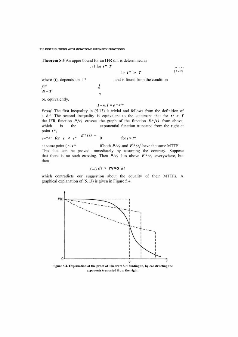
218 DISTRIBUTIONS WITH MONOTONE INTENSITY FUNCTIONS
Theorem S.5 An upper bound for an IFR d.f. is determined as . /1 for t * T „ . . .
for t * > T ( 5 ' U ) where (i)r depends on f * and is found from the condition
f t * dt = T
or, equivalently, 1 - w,T = e "<'*
Proof. The first inequality in (5.13) is trivial and follows from the definition of a d.f. The second inequality is equivalent to the statement that for t* > T the IFR function P { t ) crosses the graph of the function E* { t ) from above, which is the exponential function truncated from the right at point t * ,
e~"<' for t < t* 0 for t > t*
at some point ( < t * if both P ( t ) and E* ( t } have the same MTTF. This fact can be proved immediately by assuming the contrary. Suppose that there is no such crossing. Then P ( t ) lies above E* ( t ) everywhere, but then
r n t ) d t > rv<o d t
which contradicts our suggestion about the equality of their MTTFs. A graphical explanation of (5.13) is given in Figure 5.4.
f J
o
E* ( t ) =
Figure 5.4. Explanation of the proof of Theorem 5.5: finding to, by constructing the exponents truncated from the right.
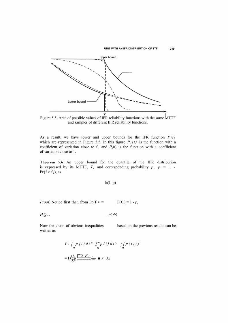
UNIT WITH AN IFR DISTRIBUTION OF TTF 219
As a result, we have lower and upper bounds for the IFR function P i t ) which are represented in Figure 5.5. In this figure P x i t ) is the function with a coefficient of variation close to 0, and Pxit) is the function with a coefficient of variation close to 1.
Theorem 5.6 An upper bound for the quantile of the IFR distribution is expressed by its MTTF, T , and corresponding probability p , p = 1 - Pr{f > £p), as
ln(l -p)
Proof. Notice first that, from Pr{f > = P(£p) = 1 - p,
H Q = «
Now the chain of obvious inequalities based on the previous results can be written as
T = [ p { t ) d t * f " p ( t ) d t > r [ p ( t p ) ] J o J o J o
f t , ['"0- P ) . = I exp .............. ... ■ x d x J n
Upper bound
Figure 5.5. Area of possible values of IFR reliability functions with the same MTTF and samples of different IFR reliability functions.
= _ln(l -/>)
220 DISTRIBUTIONS WITH MONOTONE INTENSITY FUNCTIONS
and simple integration gives us
(exp[ln(l -p)] - 1)
[ ( 1 ~ P ) ~ A
which produces the desired result.
Theorem 5.7 A lower bound for the quantile £ of the IFR distribution is expressed by T and p as
(-ln(l-p)Jr for 1 ~ p >
T for 1 - p z e
Proof. We prove the first of these inequalities separately for £p ^ T and
> T . For the first case
1 — p = P( £ p ) > e ~ l ^ ex p j - ^ j
For the second case with the use of Theorem 5.2, we immediately write
1-p-!>(*,) a
Thus, the desired inequality is valid in both cases. The second inequality, which is valid for the condition
1 - p = / > ( £ , ) < e
follows immediately if we recall (5,12). Thus,
which corresponds to the desired condition £ p > T .
l n ( l - p )
d x =expl n ( l - p )
S n
l n ( l
- p )
PtP - l n ( l - p )
■'n
1
-i
-l
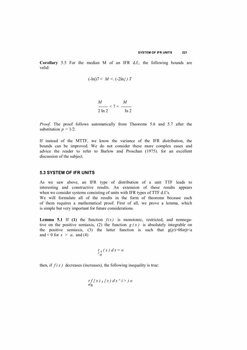
SYSTEM OF IFR UNITS 221
Corollary 5.5 For the median M of an IFR d.f., the following bounds are valid:
(-ln|)7 < M <. (-2ln{ ) T
M M ------ < 7 < ------- 2 In 2 In 2
Proof. The proof follows automatically from Theorems 5.6 and 5.7 after the substitution p = 1/2.
If instead of the MTTF, we know the variance of the IFR distribution, the bounds can be improved. We do not consider these more complex eases and advice the reader to refer to Barlow and Proschan (1975). for an excellent discussion of the subject.
5.3 SYSTEM OF IFR UNITS
As we saw above, an IFR type of distribution of a unit TTF leads to interesting and constructive results. An extension of these results appears when we consider systems consisting of units with IFR types of TTF d.f.'s. We will formulate all of the results in the form of theorems because each of them requires a mathematical proof. First of all, we prove a lemma, which is simple but very important for future considerations.
Lemma 5.1 If (1) the function f i x ) is monotonic, restricted, and nonnega- tive on the positive semiaxis, (2) the function g ( x ) is absolutely integrable on the positive semiaxis, (3) the latter function is such that g(jr)>0forjt<a and < 0 for x > a , and (4)
r g ( x ) d x = o J o
then, if f i x ) decreases (increases), the following inequality is true:
r f { x ) 8 { x ) d x ^ i > ) o •'n
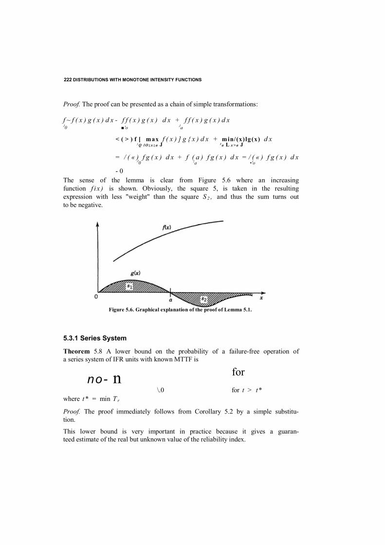
222 DISTRIBUTIONS WITH MONOTONE INTENSITY FUNCTIONS
Proof. The proof can be presented as a chain of simple transformations:
f ~ f ( x ) g ( x ) d x - f f ( x ) g ( x ) d x + f f ( x ) g ( x ) d x J0 ■'o Ja
< ( > ) f [ max f ( x ) ] g { x ) d x + min/(x)lg (x) d x } Q l O z x z a J J a L x > a J
= / ( « ) f g ( x ) d x + f ( a ) f g ( x ) d x = / ( « ) f g ( x ) d x J0 }a •'o
- 0 The sense of the lemma is clear from Figure 5.6 where an increasing function f i x ) is shown. Obviously, the square 5, is taken in the resulting expression with less "weight" than the square S 2 , and thus the sum turns out to be negative.
5.3.1 Series System
Theorem 5.8 A lower bound on the probability of a failure-free operation of a series system of IFR units with known MTTF is
no- n for \.0 for t > t *
where t * = min T r
Proof. The proof immediately follows from Corollary 5.2 by a simple substitu- tion.
This lower bound is very important in practice because it gives a guaran- teed estimate of the real but unknown value of the reliability index.
Figure 5.6. Graphical explanation of the proof of Lemma 5.1.

SYSTEM OF IFR UNITS 223
Theorem 5.9 An upper bound on the probability of a failure-free operation of a series system of IFR units with known MTTF is
1
exp(-®<j?r)
exp[-HP + < o f ) t ]
for t <; min 7] = T, 1 <.is.n
for T ^ t < T 2
for T2zt < T3
expl- £ a><?f)
V I s i z n '
where T h 1 < , i < , n , are ordered MTTFs and each <y$ is found from the equation
1 - <4>7; = exp(- ( o t f t )
Proof. The proof follows immediately from (5.13) of Theorem 5.5.
Theorem 5.10 An upper bound on the probability of a failure-free opera- tion of a series system of IFR units with known a = A(0) is
P(I! <Ta'' = exp(-r Z «;') (5-16)
for t < min T r
Proof. The proof follows immediately from Corollary 5.1.
Theorem 5.11 The MTTF of a series system of independent IFR units has the following bounds:
1
P ( t ) <
(5.15)
for t £ T
(5.17)
224 DISTRIBUTIONS WITH MONOTONE INTENSITY FUNCTIONS
r - ,min T> 1
E r Proof. An upper bound follows trivially from the obvious statement that for any t the system is less reliable than any of its units:
p,( o* n p,{ o 1
SYSTEM OF IFR UNITS 225
Therefore,
7; - f p , ( t ) d t S f n P t ( 0 d t = rsys( '0 -'o 1 si'sr
We may use Lemma 5.1 to obtain a lower bound. We show that the replacement of an arbitrary unit with an IFR distribution of TTF with a unit with an exponentially distributed TTF, which has the same MTTF, leads to a decrease of the series system's MTTF. Suppose that such a replacement is done for the «th unit of the system. We need to prove that
f n P i ( t ) d t ± fe-'T* n r , ( 0 d t J 0 liiirt J 0 JiJin-t
or, equivaiently,
A = f [ P n ( t ) - e-«T*] ]1 P A t ) d t > Q J 0 litin-l
Note that, by Theorem 5.1, Pnit) crosses expi ~ t / T„ ) once and from above and, by assumption, both these functions have the same MTTF, Thus,
p n ( l ) - e~ ' / T"
corresponds to the function of Lemma 5.1. At the same time, the function
n ^(o lilin- 1
corresponds to the decreasing function f i x ) in Lemma 5.1. Thus, by Lemma 5.1, A > 0, and the desired intermediate statement is proved. The systematic replacement of ati system units with an IFR distribution with units with a corresponding exponential distribution produces
/ 1 \ 1 rsyst s / n e ~ , / T ' d t - / exp - t E T \ d t = -------------------------------- p J 0 lsis» 0 \ 1 T { ) y
L* j i
Thus, the theorem is proved.
The upper bound can be improved if we possess additional information about the distribution P,-(f)> for example, if we know the first derivatives in t = 0 .

226 DISTRIBUTIONS WITH MONOTONE INTENSITY FUNCTIONS
Theorem 5.12 The upper bound of the series system MTTF can be written as
1 - exp — min £ ^(0)
where a, is determined from the condition
Proof. Consider an exponential distribution truncated from the right:
This distribution E * { t ) has the same MTTF as the initial distribution Pn(t). Hence, E * ( t ) crosses P n ( t ) from above (see Figure 5.7).
T < 'syst —
(5.18) L A,(0) I SiSn
-A,<0)J for
for t < , a i
t > a ,
E * ( t ) =
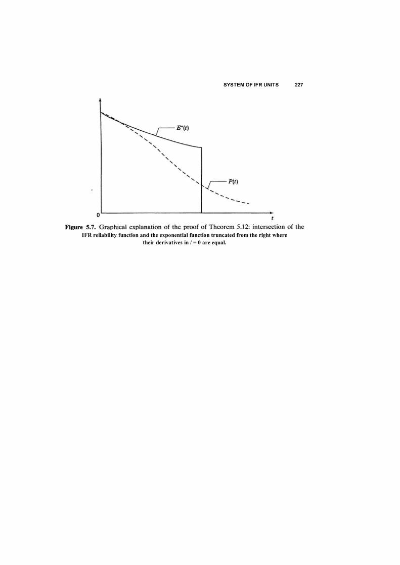
SYSTEM OF IFR UNITS 227
IFR reliability function and the exponential function truncated from the right where their derivatives in / = 0 are equal.
228 DISTRIBUTIONS WITH MONOTONE INTENSITY FUNCTIONS
In the expression for the system MTTF, replace the unit with distribution P„(t) by E*(l). The new system MTTF is
f E W ) n P , ( t ) d t = n P , { t ) d t
We now find the value of A:
A=fE*M n p L { t ) d t - r n PM d t
= H e x o ) - p n ( t ) ] n p x t ) d t
Again we can use Lemma 5.1, noticing that E * ( t ) - P„(t ) corresponds to the function g ( x ) from Lemma 5.1 and corresponds to the decreasing function from Lemma 5.1. Thus, by Lemma 5.1, A > 0, that is, the replacement of any IFR unit, say the nth, with a unit with distribution E * ( t ) might only increase the system's MTTF. Thus, the systematic replacement of units in the above-described manner leads to the final result
J 0 I
- min a{ £ A;(0)
L A,<0) 1 S i £ n
and this completes the proof.
5.3.2 Parallel Systems
Theorem 5.13 An upper bound for the probability of failure of a parallel system of IFR units can be expressed as
f F T ( 1 ~ e " / T ' ) for t £ t * Q(0 = n Qi(') * (5.19)
i s i s m I J for t > t *
where
/* = min Tj
Proof. The proof follows directly from Theorem 5.4,
d t
1 - exp

SYSTEM OF IFR UNITS 229
For the probability of a failure-free operation, the following lower bound follows from (5.19):
[ 1 - EI (l-«",/r<) for t < t * P ( t ) > I isisn. (5.20)
\ 0 for t > t *
Theorem 5.14 A lower bound for the probability of failure of a parallel system of IFR units has the form
PI [l - exp(-«(./)l for t £ t * Q ( t ) > { l i d J (5.21)
for t < t *
where
t * — max Tj 1 SfSm
Proof. The proof follows immediately from Theorem 5.5.
For the probability of a failure-free operation, the following upper bound follows from (5.21):
for t < t * n o ^ i - n [l ~ exp(-w^r)] for t > t * ( 5 - 2 2 )
1 S i S m
Theorem 5.15 The MTTF of a parallel system of independent IFR units has the bounds
1 max ij isys, i i i j . . . i i
l ^ i ' ^ r n 1 £i<j<.m __ y,
T T
1 + * • • + ( - ! ) " ' - - - y (5-23)
ISiSm i
Proof. This proof is analogous to the proof of Theorem 5.11 and so we omit it.
T, < Tiyst < £ T t ~ Z

230 DISTRIBUTIONS WITH MONOTONE INTENSITY FUNCTIONS
Again note that the lower bound is trivial and can be instantly found for a degenerate distribution, that is, for the case when ail T/s are constant.
CONCLUSION 231
Wc rtow mention that, for a parallel system, the MTTF is larger if the unit failure distributions have larger variances. (In qualitative terms, this result is close to that obtained for dependent units.) It seems paradoxical that an unstable production of some units for a parallel structure is better than a stable production: we used to think that stability is almost always better than instability. But there is no enigma at all if one notices that the random time to failure of a parallel system is the maximum of the unit's random time to failure.
Theorem 5.16 A lower bound for the MTTF of a system consisting of units with an IFR distribution, for which we know the first derivative in t — 0, is
Tjyst — E Z / 1 £ /S (B
x[l - exp(-min{7;,7}l[A,.(0) + A,(0)])]
min T , Z A , ( 0 ) Ulsm ijgij-^
Proof. The proof here is analogous to that of Theorem 5.12. We only need to notice that the probability of a failure-free operation for this case after all substitutions of P((f) for E * ( t ) has the form
p ( t ) = i — n [i- e t c ) ] lsism
where £*(/) is defined in Theorem 5.12.
5.3.3 Other Monotone Structures
Instead of writing detailed formulas with the simple substitution of IFR d.f.'s PU ) for degenerate or exponential d.f.'s, we mention only that one can obtain a lower bound for the system reliability by substituting lower bounds of the corresponding units' failure-free probabilities. Analogously, after the substitution of the upper bounds of the units' probabilities, a lower bound for the system probability is obtained. The reader can find some related results in Barlow and Proschan (1975).
CONCLUSION
This relatively new branch of reliability theory was initiated by Barlow and Proschan and became widely known after their book [Barlow and Proschan (1975)] was published. First papers on the properties of distributions with a
1
AAO)!1
+ (-1)' expz 1 sisin
232 DISTRIBUTIONS WITH MONOTONE INTENSITY FUNCTIONS
monotone failure rate appeared in the previous decade [Barlow, Marshall, and Proschan (1963); Barlow and Marshall (1964); Solovyev and Ushakov (1967); Gnedenko, Belyaev, and Solovyev (1969); among others]. We would like to present here a simple but important result concerning repairable systems [Ushakov (1966)]. The stationary interval availability co- efficient of a system with an "aging" distribution F ( t ) of TTF has lower and upper bounds of the form
^ ( 1 - 7 ) to"0'7
where K is the stationary availability coefficient and T is the mean of the distribution F ( t ) . These bounds can be easily obtained with the help of Lemma 5.1. Indeed, R ( t 0 ) for any distribution F ( t ) can be written as
*('„) - W ( t o )
where P*(t0) is the distribution of a stationary residual time:
P m ( t ) - j f ' p{ x ) d x
Substitution of degenerate and exponential d.f.'s into the latter expression and application of Lemma 5.1 produce the necessary result. This result and some others can be found in Gnedenko, Belyaev, and Solovyev (1969). Some new results can be found in Gnedenko (1983). A collection of practical results on aging units and systems consisting of aging units is presented in Ushakov (1985, 1994). This problem is especially important in practice when one possesses only very restricted statistical information but has some reasonable physical arguments about the possible behavior of a time-to-failure distribution.
REFERENCES
Barlow, R, E., and A. W. Marshall (1964). Bounds for distributions with monotone hazard rate. I and II. Ann. Math. Statist., vol. 35. Barlow, R. E., and A. W. Marshall (1965). Tables of bounds for distributions with monotone hazard rate. J. Amer. Statist. Assoc., vol. 60. Barlow, R. E., and F. Proschan (1975). Statistical Theory of Reliability and Life Testing. New York: Holt, Rinehart, and Winston. Barlow, R. E., A. W. Marshall, and F. Proschan (1963) Properties of probability distributions with monotone hazard rate. Ann. Math. Statist., vol. 34. Gnedenko, B. V., ed. (1983). Mathematical Aspects of Reliability Theory (in Russian). Moscow: Radio i Sviaz.

SOLUTIONS 233
Gen den ko, B. V., Yu. K. Belyaev, and A. D. Soiovyev (1969). Mathematical Methods of Reliability Theory. New York: Acadcmic.
Soiovyev, A. D., and I. A. Ushakov (1967). Some bounds on a system with aging elements (in Russian). Automat. Comput. Sci., no. 6.
Ushakov, 1. A. (1966). An estimate of reliability of a system with renewal for a stationary process (in Russian), Radiotekhnika, no. 5.
Ushakov, L A„ ed. (1985). Reliability of Technical Systems: Handbook (in Russian). Moscow: Radio i Sviaz.
Ushakov, I. A., ed. (1994). Handbook of Reliability Engineering. New York: Wiley.
EXERCISES
5.1 Two units have the same mean T. One unit has a uniform d.f. and another has an exponential d.f. Which one will deliver the larger probability of failure-free operation at moment / = T? At moment t = 2 T 1
5.2 Consider the Erlang d.f. of a high order (e.g., n = 10). Explain (without exact proof) how A(0 behaves.
5.3 One has to choose a system for the continuous performance of an operation during 100 hours. There are two possibilities: to choose for this purpose a system with an MTTF of 200 hours or to choose another system with an MTTF of 300 hours. Which system should be chosen.
5.4 What kind of A(r) has the system depleted in Figure E5.3?
x
x Figure E5.3.
SOLUTIONS
5.1 See Figure E5.1. 5-2 Consider a clear physical example where such a distribution appears: A
standby redundancy group of n identical and independent units. One
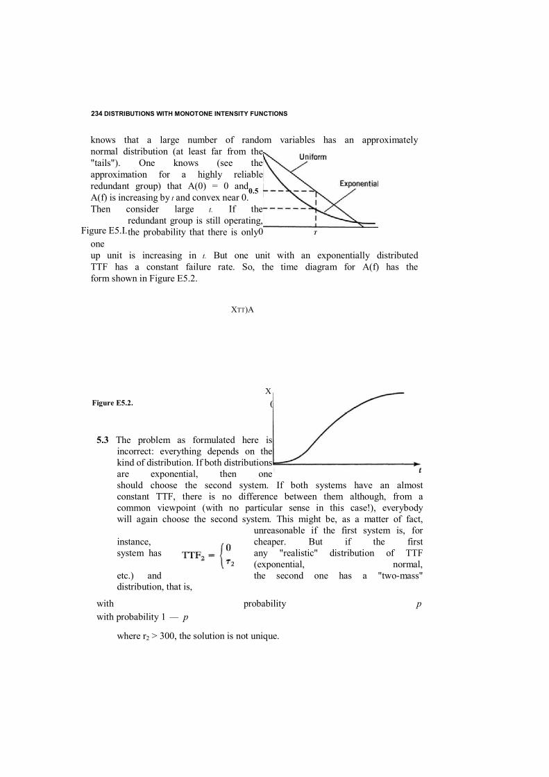
234 DISTRIBUTIONS WITH MONOTONE INTENSITY FUNCTIONS
knows that a large number of random variables has an approximately normal distribution (at least far from the "tails"). One knows (see the approximation for a highly reliable redundant group) that A(0) = 0 and A(f) is increasing by t and convex near 0. Then consider large t. If the
redundant group is still operating, the probability that there is only
one up unit is increasing in t. But one unit with an exponentially distributed TTF has a constant failure rate. So, the time diagram for A(f) has the form shown in Figure E5.2.
XTT)A
Figure E5.2.
5.3 The problem as formulated here is
incorrect: everything depends on the kind of distribution. If both distributions are exponential, then one should choose the second system. If both systems have an almost constant TTF, there is no difference between them although, from a common viewpoint (with no particular sense in this case!), everybody will again choose the second system. This might be, as a matter of fact,
unreasonable if the first system is, for instance, cheaper. But if the first system has any "realistic" distribution of TTF
(exponential, normal, etc.) and the second one has a "two-mass" distribution, that is,
with probability p with probability 1 — p
where r2 > 300, the solution is not unique.
0.5
T 0Figure E5.I.
X0
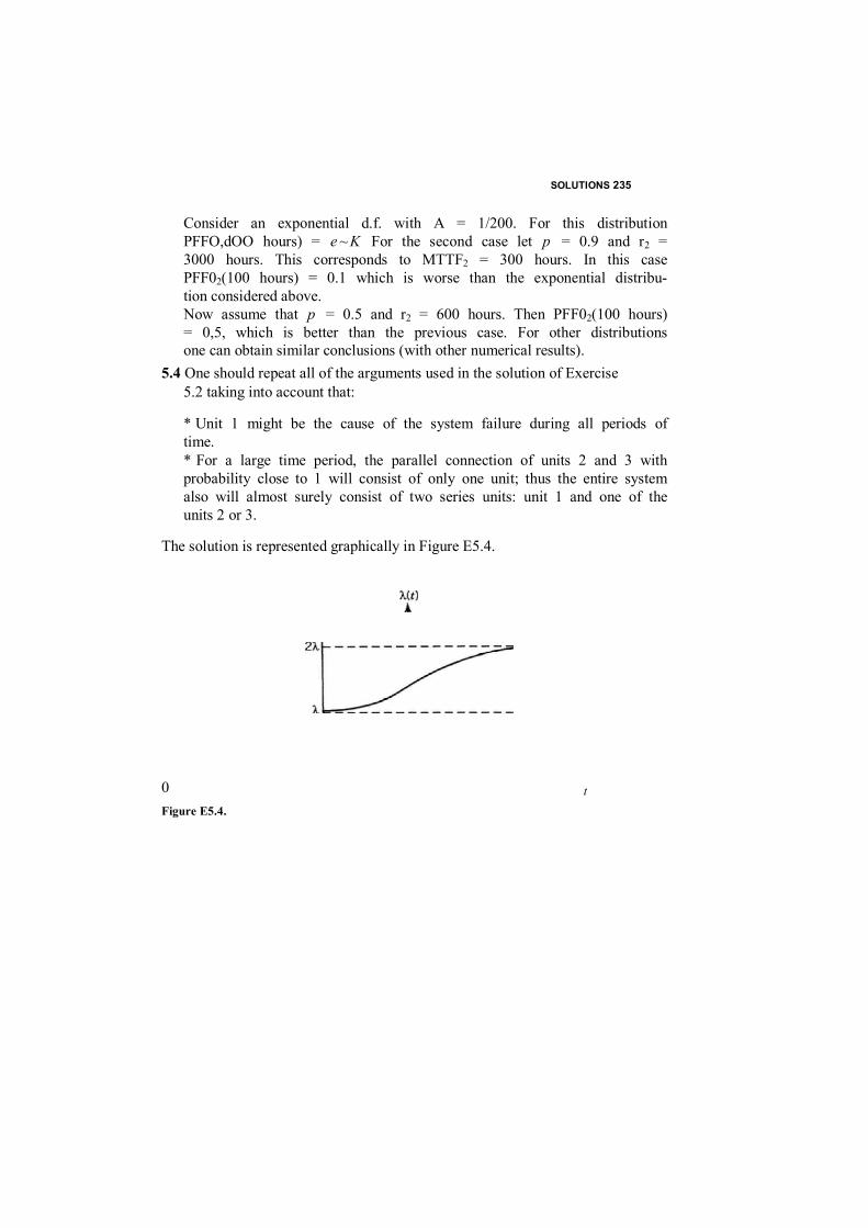
SOLUTIONS 235
Consider an exponential d.f. with A = 1/200. For this distribution PFFO,dOO hours) = e ~ K For the second case let p = 0.9 and r2 = 3000 hours. This corresponds to MTTF2 = 300 hours. In this case PFF02(100 hours) = 0.1 which is worse than the exponential distribu- tion considered above. Now assume that p = 0.5 and r2 = 600 hours. Then PFF02(100 hours) = 0,5, which is better than the previous case. For other distributions one can obtain similar conclusions (with other numerical results).
5.4 One should repeat all of the arguments used in the solution of Exercise 5.2 taking into account that:
* Unit 1 might be the cause of the system failure during all periods of time. * For a large time period, the parallel connection of units 2 and 3 with probability close to 1 will consist of only one unit; thus the entire system also will almost surely consist of two series units: unit 1 and one of the units 2 or 3.
The solution is represented graphically in Figure E5.4.
0 Figure E5.4.
t
CHAPTER 6
REPAIRABLE SYSTEMS
In engineering practice, one of the most important objects under investiga- tion is a repairable system. In general, repairable systems might be analyzed with the help of Monte Carlo simulation. There are no essential analytical results for the most general mathematical models cxcept for some very particular cases. The most important analytical models frequently used in practicc are Markov models. For these models all the system units' random TTFs and repair times are assumed to be exponential. (More accurately, each random duration of being in any state has an exponential distribution.) These assumptions might be far from valid, and so each time their appropriateness must be carefully considered. Note that if the suggestion about exponentially distributed TTFs is admissible (especially for electronic equipment), it seems artificial for the repair time. Indeed, the residual repair time should depend on the time already spent. We have discussed this issue earlier. But as we will show below, sometimes the assumptions of a distribution's exponentiality produce acceptable numerical results that can be utilized in engineering design. At any rate, Markov models are very popular for practical engineer- ing problems because of their clarity and mathematical simplicity.
6.1 SINGLE UNIT
6.1.1 Markov Model We first consider the simplest possible repairable system: a single unit. At any moment in time, the unit is in one of two states: it is either operating or 216
Probabilistic Reliability Engineering. Boris Gnedenko and Igor Ushakov
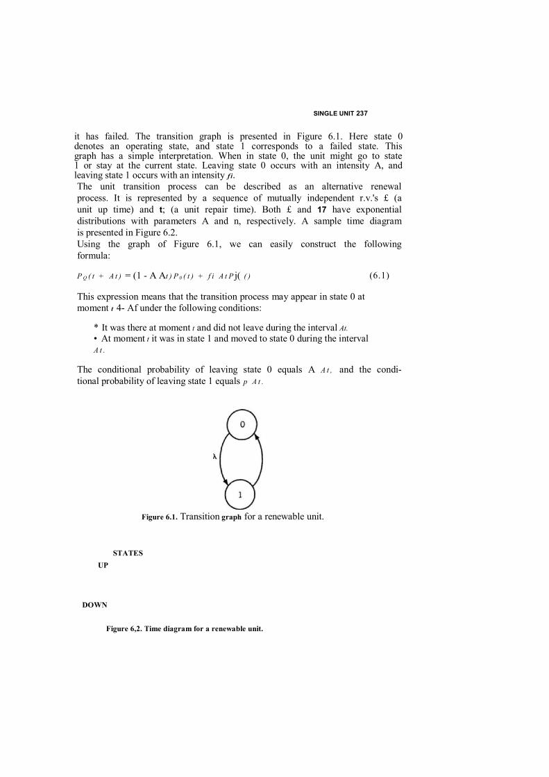
SINGLE UNIT 237
it has failed. The transition graph is presented in Figure 6.1. Here state 0 denotes an operating state, and state 1 corresponds to a failed state. This graph has a simple interpretation. When in state 0, the unit might go to state 1 or stay at the current state. Leaving state 0 occurs with an intensity A, and leaving state 1 occurs with an intensity f i . The unit transition process can be described as an alternative renewal process. It is represented by a sequence of mutually independent r.v.'s £ (a unit up time) and t; (a unit repair time). Both £ and 17 have exponential distributions with parameters A and n, respectively. A sample time diagram is presented in Figure 6.2. Using the graph of Figure 6.1, we can easily construct the following formula:
P Q ( t + A t ) = (1 - A At ) P 0 ( t ) + f i A t P j( ( )
This expression means that the transition process may appear in state 0 at moment t 4- Af under the following conditions:
* It was there at moment t and did not leave during the interval At. • At moment t it was in state 1 and moved to state 0 during the interval A t .
The conditional probability of leaving state 0 equals A A t , and the condi- tional probability of leaving state 1 equals p A t .
Figure 6.1. Transition graph for a renewable unit.
STATES
Figure 6,2. Time diagram for a renewable unit.
(6.1)
UP
DOWN

238 REPAIRABLE SYSTEMS
From (6.1) we obtain
p0(t + t o ) - p 0 ( t )
A t
Jn the limit as A t —► 0, we obtain
^-P0{t) = -A P0(r) +/*/>,(') tfc
This represents the simplest example of Kolmogorov's equation. This equa- tion expresses a condition of dynamic equilibrium. To solve it with respect to any P k ( t ) , we need to have one more equation. It is clear that another equation cannot be obtained in the same manner: it would be linearly dependent on the first one and, consequently, would not be useful in obtaining the solution. The second equation which should be chosen is the so-called normalization equation:
P o ( < ) + P i ( 0 - 1
which means that at any moment the unit must be in one of two possible states. We also need to determine the initial condition for the solution of the system of differential equations. In this simple case the problem can easily be solved in general when P 0 ( t 0 ) = p and, consequently, P£t0) = q, p + q — 1. This problem can be solved with the help of different methods. We will use the Laplace-Stieltjes transform (LST) to make the presentations in the book uniform. Recall that the LST <p(.0 of the function f i t ) is defined as
(6.5)
(In this context we consider functions f i t ) defined over the positive axis.]
Nonstationary Availability Coefficient The system (6.2) and (6.4) for this case has the LST:
~ P + - * < Po ( 0 = ™ A < Po ( 0 + f K Pl ( 0 1
<p0(O + = -
-A P 0 ( t ) + f i P . O ) (6.2)
(6.3)
(6.4)
(6.6)
(6.7)

SINGLE UNIT 239
or, in canonical form,
(A + s ) < P 0 i s ) - wi s ) =p s<Po(s) + 5<Ps(0 = 1
240 REPAIRABLE SYSTEMS
Thanks to the LST, the system of linear differential equations turns into a system of algebraic equations. To solve (6.7), we can use Cramer's rule:
To invert this LST, we have to present it in the form of a sum of terms of type a / s or b / ( s + a). The inverse functions for these terms are a constant and an exponential function, respectively.
To present the solution (6.8) in the desired form, we should find the roots of the denominators of (6.8). They are: = 0 and s 2 — -(A + p). Now we can write
A = — +
s + A + f t
where A and B are the unknown constants to be determined. To find them, we should note that two polynomials with similar denominators are equal if and only if the coefficients of their numerators are equal. Thus, we set the two
representations equal: A B s A + p + s s(A + ( i + s)
And so we obtain a new system for A and B by equalizing the coefficients of the polynomials:
A + B - p A ( A + p) - p
It is easy to find
A = A + p.
k p - p , { \ ~ p ) B = p —
A + p . A + p
P
1 5 p s + p .
A + s - p s 2 + (A + f t ) s s s
<Po(s) = (6.8)
BB
<Po(*) = (6.9)
s ~ s , 5 - 5 ,
PS + p
(6.10)
(6.11)
(6.12)

SINGLE UNIT 241
Thus, the LST of interest can be written as M
£ A p - - p ) A + p + s
V -
< P o ( s ) (6.13)A + p . s A + p.
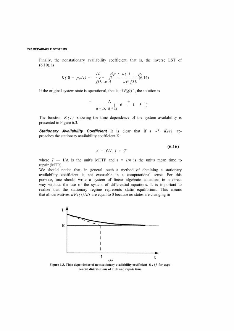
242 REPAIRABLE SYSTEMS
Finally, the nonstationary availability coefficient, that is, the inverse LST of (6.10), is
I L A p ~ u ( 1 — p ) K ( 0 = p 0 ( t ) = —~-r + —ji -------------------(6.14)
f j L ~R A A T" f J L
If the original system state is operational, that is, if Pa(t) 1, the solution is
= - A - + — — ( 6 . 1 5 ) A + fx, A + fi
The function K ( t ) showing the time dependence of the system availability is presented in Figure 6.3.
Stationary Availability Coefficient It is clear that if t - * K ( t ) ap- proaches the stationary availability coefficient K:
(6.16) A + f J L 1 + T
where T — 1/A is the unit's MTTF and r = 1/n is the unit's mean time to repair (MTR). We should notice that, in general, such a method of obtaining a stationary availability coefficient is not excusable in a computational sense. For this purpose, one should write a system of linear algebraic equations in a direct way without the use of the system of differential equations. It is important to realize that the stationary regime represents static equilibrium. This means that all derivatives d P k ( t ) / d t are equal to 0 because no states are changing in
A+P Figure 6.3. Time dependence of nonstationary availability coefficient K i t ) for expo-
nential distributions of TTF and repair time.
SINGLE UNIT 243
time, "on the average." Consequently, all Pk's must be constant. It is also clear that the initial conditions (the original state of the unit at moment / = 0) also will not make any sense. This assumption leads directly to the following system of algebraic equations:
-A P a + = 0
P 0 + F , = 1
where
P k - h m P k ( t )
are the stationary probabilities of interest. Again, the solution can be obtained with Cramer's rule
Of course, we mention Cramer's rule not as a computational tool, but rather as a methodological reference. Everyone might choose his or her own method for this particular computational task.
Probability of a Failure-Free Operation Considering previous reliability indexes, we assumed that both unit states are transient. But if one needs indexes such as the probability of a failure-free operation during a specified time interval, or the MTTF, the transition graph should be reconstructed. In these cases the unit failure state has to be absorbing. The transition graph for this case is presented in Figure 6.4. There is no transition from state 1 back to state 0, that is, fi = 0. In this case we have the
(6.17)
(6.18)
0 fL
1 1
-A ( i
1 1 A + ( i T + t
P0 = K = (6.19)
6

244 REPAIRABLE SYSTEMS
0 Figure 6.4. Nontransitive graph for computation of the MTTF of a renew- able unit with an exponentially distributed TTF.
SINGLE UNIT 245
equation
~ P 0 ( t ) = ~ X P 0 ( t ) (6.20)
This differential equation can again be solved with the help of the LST. First, we write the following algebraic equation with the natural initial condition P0it) » 1:
-1 + s<p0(i) = -A<p0($)
(6.2
1)
and then solve it to obtain
W
(6.22
) Mean Time to Failure To find the unit's MTTF, we should recall that the mean of nonnegative r.v.'s can be found as
E { X } = [ ~ P( x ) d x (6.23) A)
where P i t ) = 1 - F i t ) . Using the previous notation, we take P i t ) = P 0 i t ) . At the same time, we can write
E{*} = f>(*)e_JW<fcUo o
It follows that, to find the MTTF, we can use the solution for P0it) in terms of the LST and substitute s = 0. In fact, it is even sometimes simpler to solve a corresponding system of equations directly with the substitution 5 = 0.
Considering a single unit, there is no technical difference: = - (6.25)
j — 0 A
1 T*=
A + j

246 REPAIRABLE SYSTEMS
Notice that if we need to find the MTR, it is necessary to start from state 1 and choose state 0 as absorbing.
We present an in-depth analysis of this simple case in order to make future explanations of more complex models more understandable. We do this to avoid explanations below with unnecessary additional details. The same purpose drives us to use a homogeneous mathematical technique for all routine approaches (though, in general, we try to use various methods because our main purpose is to present ideas and not results).
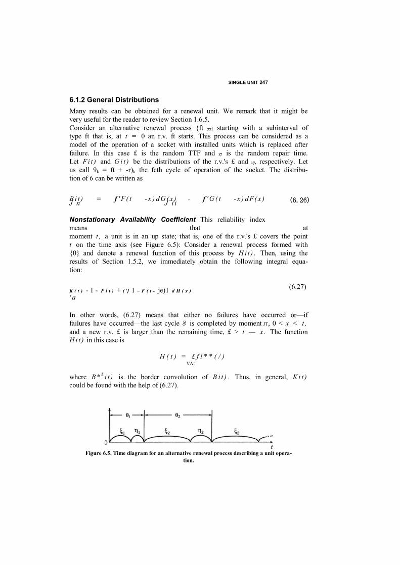
SINGLE UNIT 247
6.1.2 General Distributions Many results can be obtained for a renewal unit. We remark that it might be very useful for the reader to review Section 1.6.5. Consider an alternative renewal process {ft 77} starting with a subinterval of type ft that is, at t = 0 an r.v. ft starts. This process can be considered as a model of the operation of a socket with installed units which is replaced after failure. In this case £ is the random TTF and 17 is the random repair time. Let F i t ) and G i t ) be the distributions of the r.v.'s £ and 17, respectively. Let us call 9k = ft + -r)k the fcth cycle of operation of the socket. The distribu- tion of 6 can be written as
B i t ) = f ' F ( t - x ) d G (x ) = f ' G ( t - x ) d F( x ) J n J i i
Nonstationary Availability Coefficient This reliability index means that at moment t , a unit is in an up state; that is, one of the r.v.'s £ covers the point t on the time axis (see Figure 6.5): Consider a renewal process formed with {0} and denote a renewal function of this process by H i t ) . Then, using the results of Section 1.5.2, we immediately obtain the following integral equa- tion:
K ( t ) - 1 - F i t ) + ( ' [ 1 ~ F ( t - je)1 d H ( x ) ' a
In other words, (6.27) means that either no failures have occurred or—if failures have occurred—the last cycle 8 is completed by moment JT, 0 < x < t , and a new r.v. £ is larger than the remaining time, £ > t — x . The function H i t ) in this case is
H ( t ) = £ f l * * ( / ) VA:
where B * k i t ) is the border convolution of B i t ) . Thus, in general, K i t ) could be found with the help of (6.27).
(6.26)
(6.27)
Figure 6.5. Time diagram for an alternative renewal proccss describing a unit opera- tion.
248 REPAIRABLE SYSTEMS
Stationary Availability Coefficient Intuitively, it becomes clear that (6.27) has a limit when time is increasing: K ( t ) - * ■ K . (Strictly speaking, the in- volved distributions must be continuous.) Indeed, applying the Smith theo- rem (Section 1.5.2), we obtain
1 E{£}
* " fr.™ " iw /»[1 " A " iifiTlM (6'28)
On a heuristic level, this result can be explained by the following arguments. Consider some interval of time L such that the number of cycles on it n is sufficiently large. Then
The index K is the probability that an arbitrary moment will be covered by an interval of type It is clear that this probability is proportional to the total portion of time occupied by all intervals of type f:
E ii ^ E 6 j^ _ 1 <,i£n _ lsifi
E h + E V i r V T T i r „ ! s i s n 1 <Li<.n - ^ .. ^
n I£/£« n 1< i z n
and, if n is large, one may replace each sum with the coefficient 1 / n for the mean of the respective r.v.
E{£} K - m r m (6'29>
Nonstationary Interval Availability Coefficient Again, we can write the integral equation
f i (Mo) = 1 ~ F ( t + t Q ) + / ' [ 1 - F( t + t 0 ~ x ) ] d H ( x ) (6.30) o
The explanation of (6.30) is similar to the explanation of (6.27).
Stationary Interval Availability Coefficient Again, we use the Smith theorem and write
R { t 0 ) m lim = />(*)<& (6.31) ''fy
SINGLE UNIT 249
where £ is the residual time of the renewal process formed with the r.v.'s {£}. From (6.32) it becomes clear that R U 0 ) differs from ffwrong(f0) = KP{t0\ In engineering practice, nevertheless, i?wroi,g(f0) is often erroneously used. We should emphasize that £ and its residual time £ are statistically equiva- lent only for an exponentially distributed r.v. Consequently, in this case (and only in this case!),
R ( t a ) ~ K P( t 0 ) = R ( t 0 ) = K e
For a highly reliable unit, (6.32) can be written in the convenient form of two-sided bounds if F i t ) is "aging." For this purpose we use a result from Chapter 5. Recall that
where F ( t ) is an "aging" distribution with mean T and D T U ) is a degenerate distribution, that is, a constant T , Then it follows that
where f is the residual value of the renewal process formed with {£}. For a highly reliable unit, we can write a very simple and very convenient approximation
P( * o ) = 1 ~
Thus, for the index of interest, we write
(6.33)
and for a highly reliable unit
It is convenient to rewrite (6.31) in the form
T
250 REPAIRABLE SYSTEMS
(6.34)

REPAIRABLE SERIES SYSTEM 251
6.2 REPAIRABLE SERIES SYSTEM
6.2.1 Markov Systems Consider a series system of n independent units. Assume that distributions of the TTF, Fj(t), and distributions of the repair time, G(0), are exponential:
F ( t ) - 1 - e~x' G ( t ) « 1 -
Here A, and n, are the parameters of the distributions, or the intensities of failure and repair, respectively.
Reliability indexes depend on the usage of the system's units during the system's idle time. We consider two main regimes of system units in this situation:
1. After a system failure, a failed unit is shipped to a repair shop and all of the remaining system units are switched off. In other words, the system failure rate equals 0 during repair. In this case only one repair facility is required and there is no queue for repair.
2. After a system failure, a failed unit is shipped to a repair shop but all the remaining system units are kept in an operational state. Each of them can fail during the current repair of the previously failed unit (or units). In this case several repair facilities might be required. If the number of repair facilities is smaller than the number of system units, a queue might form at the repair shop.
System with a Switch-Off During Repair The transition diagram for this system is presented in Figure 6.6. We will not write the equations for this case. As much as possible, we will try to use simple verbal explanations.
Figure 6.6. Transition graph for a series system which is switching oif during idle time.
252 REPAIRABLE SYSTEMS
1. Probability of Failure-Free Operation
Any exit from state 0 leads to failure. Hence,
/>(/) = exp(- £ A,7)=«rA' (6.35) ^ 1 si sn '
where
A = I 1 sisn
Thus, by this reliability characteristic, the system is equivalent to a single unit with a failure rate A.
2. MTTF
If P i t ) = e ~ A l , the MTTF of the system equals Tsyst = 1/A. No comments are needed.
3. Mean Repair Time
Let us consider a general case where all units differ by their repair time 1 /n(. The current repair time of the system depends on which unit has failed. The distribution of the system's repair time can be represented in the form
Pr{77 ^ / } = £ p k e (6.36)
where p k is the probability that the /cth unit is under repair. The probability p k can be easily found as
A* Pk = ^ A (6.37)
J SLS/L
Notice that the distribution of the system's repair time has a decreasing intensity function; that is, with the growth of the current repair time, the residual repair time becomes larger and larger.

REPAIRABLE SERIES SYSTEM 253
We consider this phenomenon in more detail. Write (6.36) in the form
(0 - E />*^' = exp(- f ' p ( x ) d x ) r
1 Sk < . n
From here we find
d r ( t ) Z HtPke-*" M } r { t ) d t Z Pke~»"
1 s . k < , n
Now we note that f i ( t ) is a monotone function. For t = 0, a simple qualita- tive analysis gives us
Z v-kPk = - - - - - - - - - - - „ £ p . k p k ~ E ( p }
i — P k l ^ k &n J S I S N
Now, as t oo,
, . P-k*Pk> im MO = „
where /c * corresponds to the subscript of a minimal fik. Obviously, the average value is larger than the minimum. This function is never below the minimal Hence, n . ( t ) decreases from the average value of p at f = 0 to the minimal value among all ji's. It can be shown that this decrease is monotone. Of course, from (6.36) and (6,37), it follows immediately that
Tsyst ~ syst} ~ E T i y , A 1 ' I
1 iiin
where T(- = l/PT; is the MTTF of the ith units.
4. Nonstationary Availability and Interval Availability Coefficients
We are able to find these reliability indexes only with the help of general methods of renewal process theory, in spite of the exponentiality of a TTF distribution. One can also use standard Markov methods applied to the

254 REPAIRABLE SYSTEMS
transition graph presented in Figure 6.6. The corresponding system of equa-
REPAIRABLE SERIES SYSTEM 255
tions for the availability coefficient is
no - - n M * ) + *k Po ( t ) 1
= 1 taken for 0 £ k n
and the initial condition P0(0) = 1. We will not solve these equations here. But if K ( t ) is found, then—because of the exponentiality of the TTF distribution—R ( t , t 0 ) = K ( t ) e ~ A ' .
5. Stationary Availability Coefficient
With known 2"syst and rsyst, this index can be found in a standard way as K = (Tsys,)/(7LSI + rsyst). Note that in this particular case it is convenient to write
K = 1 (6.38) 1 + L A ,r,
1 sirsn
6. Stationary Interval Availability Coefficient
Because of the exponential distribution of the system TTF, we can use the expression R ( t 0 ) = K P( t 0 ) where P ( t 0 ) is defined in (6.35). Notice that if all arc constant (equal to fi), the above-described system is transformed into a single repairable unit with an intensity of failure equal to
A - E A, 1 rsiin
and an intensity of repair n. In most practical cases it is enough for the first stages of design to put /J. - E{/x} in this model and to use this approximation instead of using the exact model. We remark that in most practical cases, when the equipment has a modular construction, the mean time of repair might be considered almost equal for different system units. But an even more important argument for such a suggestion is that a mathematical model must not be too accurate at the design stage when one does not have accurate input data.
System Without Switch-Off During Repair First, consider a series system of n different repairable units when there are n repair facilities in a workshop; that is, each unit might be repaired independently. The units' failures are assumed independent. In this case the system can be considered
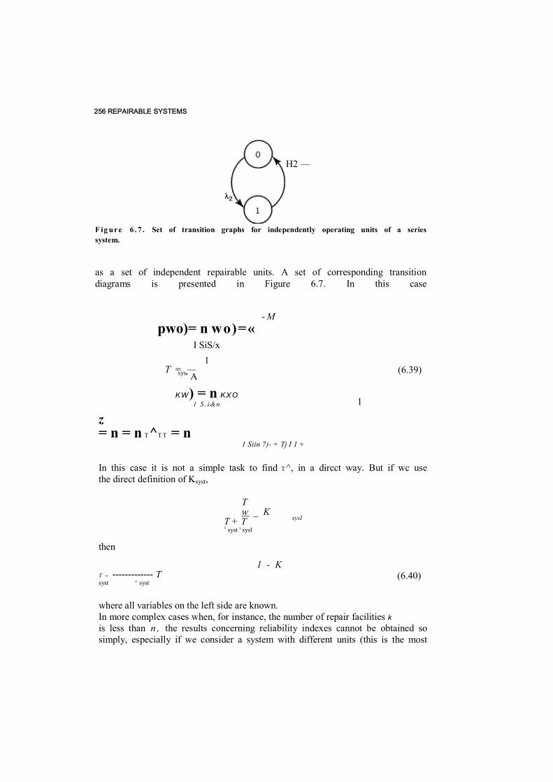
256 REPAIRABLE SYSTEMS
F ig ur e 6 .7 . Set of transition graphs for independently operating units of a series system.
as a set of independent repairable units. A set of corresponding transition diagrams is presented in Figure 6.7. In this case
pwo)= n wo)=« I SiS/x
1 T = — sys' A
KW) = n KXO 1 S . i &n
z = n = n T^T T = n
1 Siin 7)- + Tj I 1 +
In this case it is not a simple task to find T^, in a dircct way. But if wc use the direct definition of Ksyst,
T w _ K
T + T sysI 1 syst ' sysl
then
1 - K T - ------------- T syst ^ syst
where all variables on the left side are known. In more complex cases when, for instance, the number of repair facilities k is less than n , the results concerning reliability indexes cannot be obtained so simply, especially if we consider a system with different units (this is the most
H2 —
- M
(6.39)
(6.40)
1

REPAIRABLE SERIES SYSTEM 257realistic practical case, by the way). In this case there is no way other than to construct a transition graph, to write a system of linear differential equations, and then to solve them.
258 REPAIRABLE SYSTEMS
6.2.2 General Distribution of Repair Time If the TTFs of all the units remain exponentially distributed, the main simple results can be obtained practically in the same form as for the Markovian model.
System With Switch-Off During Repair First of all, fsyst(/0) and Tsys, remain the same as in the previous case. The mean repair time is defined with the help (6.36). Consequently, the stationary availability and interval availability coefficients can be expressed in standard form. At the same time, nonstationary indexes can be found with the help of the general methods of renewal process theory. The model of the investigated operation process forms an alternative process {£*, T J *}. Each is an exponential r.v. with parameter A and 17* is an r.v. with a complex "weighted" d.f.
G * ( / ) - P r { , T < £ / } - - E A , G , ( 0 A 1Z i Z n
For analytical purposes it is more reasonable to use Monte Carlo simula- tion. We would like to emphasize again that a detailed exploration of a nonstationary regime is usually a task far removed from practical needs becausc of the insufficiency of the input data.
Sysfem Without Switch-Off During Repair In this case Psyst(f0) and Tsysl remain the same as in the previous cases. Even such a stationary index as K can be found only for the case when the number of repair facilities equals the number of system units, that is, when all system units are totally independent. In this case K is defined as
1 ^ _ ___________
1 ^sysl^syst
If the system units are dependent through the lack of repair facilities, we recommend the use of Monte Carlo simulation for the computation of nonstationary indexes.
But if K or K i t ) is known, to find R ( t 0 ) or R ( t , t 0 ) is a simple task because of the exponentiality of the system TTF: R ( t 0 ) = K P( t 0 ) and R ( t , t 0 ) = K ( t ) P( t { } ) .
6.2.3 General Distributions of TTF and Repair TimeThis case is especially difficult if one considers nonstationary indexes. They can only be found with the help of Monte Carlo simulation. Let each unit of the system be described with the help of an alternative renewal process. The

REPAIRABLE REDUNDANT SYSTEMS OF IDENTICAL UNITS 259 superposition of these processes is not an alternative renewal stochastic process. The new process has more sophisticated structure: it does not have the regeneration moments that appeared when one considered a system of units with exponential TTF.
But to find the stationary coefficient K , we can use the idea that stationary probabilities do not depend on the distribution of the repair time. Therefore, one can use a Markov model with the following parameters for each unit:
11 11 A . = ----------------------------------- and f [ 1 - F , ( t ) ] d t T > / [l-Gf(f)I
'ii i'n
If the number of repair facilities equals the number of system units (all units are totally independent), the system stationary availability coefficient can be found as
T> 1 s i s t li * ~i
The stationary interval availability coefficient can also be found with the help of the following arguments. For each unit we can easily find the conditional stationary probability of a failure-free operation under the condition that a unit is in an operational state at the starting moment:
1 ,» = Pr{£ * f0} =-/ P ( x ) d x
* i %
Then for the system
i S/Sn 1i ^ ~i
Now it is possible to write J?(r0) as
I I S i S n ' i + Ti 'u
Also, we can again use the two-sided bounds (6.33) if the unit TTF distribu-
tions are "aging":
n — n — ^ - e x p ( - r 0 Z ^ f I
Isi'sn 1 4. — \ * i f I SIS" 1 + — \ l s i s n l i )
(6.41)
Z dt
^ C oJ - ^ ^ C o) - n ytt fp'(x)dx
260 REPAIRABLE SYSTEMS
Naturally, using (6.34) for a highly reliable system, we can write
*syst('o) = l- £ (6-42) l^i^rt i
Of course, analogous approximations could be written for all of the above- considered cases in this section.
6.3 REPAIRABLE REDUNDANT SYSTEMS OF IDENTICAL UNITS
6.3.1 General Markov Model Let us consider a redundant system consisting of k main operating units and n = n } + n 2 + redundant units. Here we use the following notation:
• «[ is the number of active redundant units in the same regime as the main operating units; each unit has a failure rate A;
• n2 is the number of units in an underloaded on-duty regime; each unit has a failure rate A', A' = v \ , where v is the so-called loading coeffi- cient, 0 < v < 1;
- n3 is the number of standby units; each unit has A" = 0.
A failed unit is shipped to the repair shop. A failed operating unit is replaced with an active redundant unit. Instantly, this unit is replaced by a unit which is in an underloaded regime, and, in turn, the latter is replaced by a standby unit. An analogous chainlike procedure is performed with a failed unit of other levels of redundancy. There are I repair facilities, 1 < , I <: n + k . All units have an exponential repair time distribution with the same parame- ter /i.
Let Hj denote a system state with j failed units. Obviously, the system can change its state Hj only for one of two neighboring states: HJ_l after the repair of a failed unit or H J + 1 after a new failure. Hence, this process is described with the help of a linear transition graph (see Figure 6.8) and belongs to the birth and death process (sec Section 1.6).
The transition from state H } to state H j + l within a time interval [t , t + A ] occurs with probability A j A t + o ( A t ) . The transition to state H j _ { in the same time interval occurs with probability M j A t + o ( A t ) . With probability 1 - A, A t - M j A t — o ( A t ) , no change occurs. For underloaded units, the coefficient of loading is v , 0 < v < 1.
A system with n redundant units has n + k + 1 states H 0 , H \ , H 2 , . .., H n + k . States H n + j with n + j failed units, 1 < j < k , are states corresponding to a system failure. After an exit into the first system failure state, H n + l , the process develops further: it may move to the next

REPAIRABLE REDUNDANT SYSTEMS OF IDENTICAL UNITS 261 (a) (b)
Figure 6.8. Two linear transition graphs for a redundant system: (a) without an absorbing state; (ft) with an absorbing state.
system failure state, H n + 2 , and so on, or it may return to the up state, H n . If the state Hn + ] is absorbing, the system of equations must be changed: all absorbing states must have no transition to the set of
operational states. This new system of equations can be
used for calculating the probabilities of successful operation, the interval availability coefficient, the MTTF, and the MTBF.
If we consider the nonstationary and
stationary availability coefficients, the stale Hn+k is reflecting. The corresponding system of equations can be used
for calculating the nonstationary availability and/or interval availability co- efficients.
N- 1-1 N~ 1 - 1
States of > the system's
failure
State of the system's failure

262 REPAIRABLE SYSTEMS
Considering the transition graph without an absorbing state, for a state H j r
0 <;'<«= n, + «2 + n i + k , one may write Ay and M f .
A0 = k X + «,A + n 2 v X A, = /cA + n, A + n 2 v X = A0
= Ao
A„i+, = k X + n, A + («2 — 1)PA
A„i+2 = &A + rtj A + («2 — 2 ) u X
An.,+„2 = *A + «,A
A „ 3 + „ 2 + , = k \ + ( n , - 1 ) A
Anj+fl2+2 = + ("i - 2)A
AMj + n2 + n, = ^A
A n , + n 2 + n ,+ l = ( k ~ 1 ) A
AH,+«a+n,+ 2 = (* ~ 2)A
A/i|+n2 + n3 + A
and for all M j , 0 < j < n + k = n x + n 2 + n3 + k ,
Mj = n, M2 = 2 / J L , . . . , M, = In, M,+ ] = l n , . . . , M n + k = l p The system with the absorbing H n + X state is the system which operates until a first failure. This system can be analyzed with the following system of differential equations:
d p j ( t ) - A , _ , / > , _ , ( * ) - ( A y + M j ) p j ( t ) + M j + i P j + i ( t ) 0 < j z n + 1
(6.43) A_, - A„ + 1 = A/0 = A/fl = ••• =A/n+, = 0 (6.44)
where P j ( t ) is the probability that the system is in state H t at moment t . The normalization condition is
E PA O = i 0s/sn+1
GENERAL MARKOV MODEL OF REPAIRABLE SYSTEMS 263The system with the reflecting Hn+k state can be described by the
following system of differential equations:
d p i t )
~~di~ = V i * / - i ( 0 ~ ( A j + M j ) p j ( 0 + M j + i P f + t ( 0 0 < j < n + k
A^, = An+Jt = M0 - Mn+k+l « 0
with normalization equation
E MO = 1
Because our goal is not to write down formulas for very general models but to show the methodology and methods, we hope that the reader can use the corresponding equations from Section 1.6 dedicated to the death and birth process.
Precise formulas for such a general case are almost always long and complicated. If one deals with highly reliable systems, we recommend the reader refer to Chapter 12. (If one deals with an unreliable system, we recommend a redesign of the system, not a useless calculation!)
The next section is devoted to general methods of analysis of repairable systems.
6.4 GENERAL MARKOV MODEL OF REPAIRABLE SYSTEMS
6.4.1 Description of the Transition Graph From the very beginning, we would like to emphasize that a Markov model is an idealization of a real process. Our main problem is not to solve the system of mathematical equations but rather to identify the real problem, to deter- mine if the real problem and the model are an appropriate fit to each other. If, in fact, they are a good fit, then a Markov model is very convenient.
Now let us assume that we can construct the transition graph which describes a system's operation. This graph must represent a set of mutually exclusive and totally exhaustive system states with all of their possible one-step transitions. Using some criterion of system failure, all of these states can be divided into two complementary disjoint subsets, up states and down states. A transition from the subset of up states to the subset of down states may occur only when an operating unit fails. An inverse transition may occur only if a failed unit is renewed by either a direct repair or by a replacement. Let us consider a system with n units. Any system state may be denoted by a binary vector
s - (*!,..., sn)

264 REPAIRABLE SYSTEMS
where s i is the state of the z'th unit. We set s( = 1 if the unit is operational and s■ = 0 otherwise. The transition from ( .s l , . . . ,s i = 1,...,s n ) to (5,,,.., 5, = 0,..., s n ) means that the /th unit changes its state from up to down. The transition rate (or the transition intensity) for this case equals the /th unit's failure rate.
A transition from system state (s,,,.., = 0,.,., .?„) to state (5,,..., Sj = 1,..., s„) means that the /'th unit was in a failed state and was renewed . The transition rate for this case equals the 1 th unit's repair rate. These kinds of transitions are most common. For Markovian models we assume that only one unit may fail (or be renewed) at a time. (If several units may change states simultaneously, for example, under a group repair, we will consider this separately.) Of course, there are other possible interpretations of states and transitions. For instance, s, = 1 may be a state before monitoring or switching, and s, = 0 is the same state after the procedure. We denote these transitions from state to state on transition graphs with arrows. The rates (intensities) are denoted as weights on the arrows. The graph structure is determined by the operational and maintenance regime of the system's units and the system itself. After the transition graph has been constructed, it can be used as a visual aid to determine different reliability indexes. An example of such a transition graph for a system consisting of three different units is presented in Figure 6.9.
6.4.2 Nonstationary Coefficient of Availability Let E ( k ) denote the subset of the entire set of system states which includes states from which a direct transition to state k is possible, and let e ( k ) denote the subset to which a direct transition from state k is possible. The union E ( k ) U e ( k ) is the subset of system states that have a direct connec- tion to or from state k (see Figure 6.10). For each state k of the transition graph, we can write the following differential equation:
d 0 = "M O £ Alk + £ A i k P i ( t ) (6.45)
a l i ^e(k) / e£(A )
where Aik is the intensity of the transition from i to k, and p,(f) is the probability that the system is in state //, at moment t.
The transition graph and the system of differential equations can be interpreted as those which describe a dynamic equilibrium. Indeed, imagine that each node i is a "basin" with "liquid" which flows to each other node j (if there is an arrow in the corresponding direction). The intensity of the flow is proportional to Au (specified in each direction) and to a current amount of "liquid" in the source P J( t ) .
If there are n states, we can construct n differential equations. To find the nonstationary coefficient of availability, we take any n — 1 equations, add the

GENERAL MARKOV MODEL OF REPAIRABLE SYSTEMS 265
normalization condition
L PiO) = 1 (6-46) I
and add initial conditions of the type p f ( 0) = p t where p,-(0) is the probability that the system is in state i at t = 0. In turn, the p/s are probabilities that conform to a normalization condition similar to (6.46). If Pi =■ I for some i, then p j = 0 for all j , j + i . In most problems the initial system state is the state when all units are up. To find the nonstationary availability coefficient, we can use the Laplace-Stieltjes transform (LST). Then the system of n linear differential
Figure 6.9. Transition graph for a system consisting of three different renewable units.
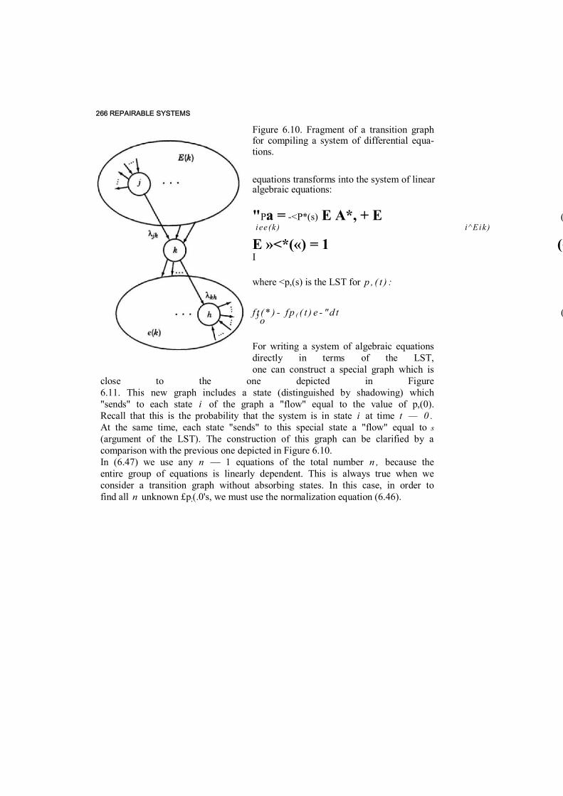
266 REPAIRABLE SYSTEMS
Figure 6.10. Fragment of a transition graph for compiling a system of differential equa- tions.
equations transforms into the system of linear algebraic equations:
"Pa = -<P*(s) E A*, + E (6.47)i ee(k) i ^Eik)
E »<*(«) = 1 (6I
where <p,(s) is the LST for p , ( t ) :
f t ( * ) - f p ( ( t ) e - "d t (6.49)J o
For writing a system of algebraic equations directly in terms of the LST, one can construct a special graph which is
close to the one depicted in Figure 6.11. This new graph includes a state (distinguished by shadowing) which "sends" to each state i of the graph a "flow" equal to the value of p,(0). Recall that this is the probability that the system is in state i at time t — 0 . At the same time, each state "sends" to this special state a "flow" equal to s (argument of the LST). The construction of this graph can be clarified by a comparison with the previous one depicted in Figure 6.10. In (6.47) we use any n — 1 equations of the total number n , because the entire group of equations is linearly dependent. This is always true when we consider a transition graph without absorbing states. In this case, in order to find all n unknown £p;(.0's, we must use the normalization equation (6.46).
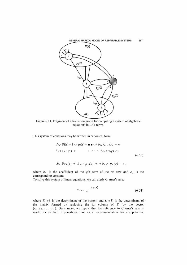
GENERAL MARKOV MODEL OF REPAIRABLE SYSTEMS 267
This system of equations may be written in canonical form:
f>n<Pi(s) + f>„<p2(s) + ■ ■ • + b l n ( p „ ( s ) = ct
b 2 l < Pl ( s ) + + ' ' ' +b2n<Pn(s) = C2 (6.50)
& n l ¥ » i ( j ) + b n 2 < p 2 ( s ) + + b n n < p n ( s ) - c „
where b u is the coefficient of the yth term of the rth row and c { is the corresponding constant. To solve this system of linear equations, we can apply Cramer's rule:
Z)j(s) *<•> - m (6-51)
where D ( s ) is the determinant of the system and £>,(5) is the determinant of the matrix formed by replacing the ith column of D by the vector (c(, c 2 , . . . , c „ ). Once more, we repeat that the reference to Cramer's rule is made for explicit explanations, not as a recommendation for computation.
Figure 6.11. Fragment of a transition graph for compiling a system of algebraic equations in LST terms.
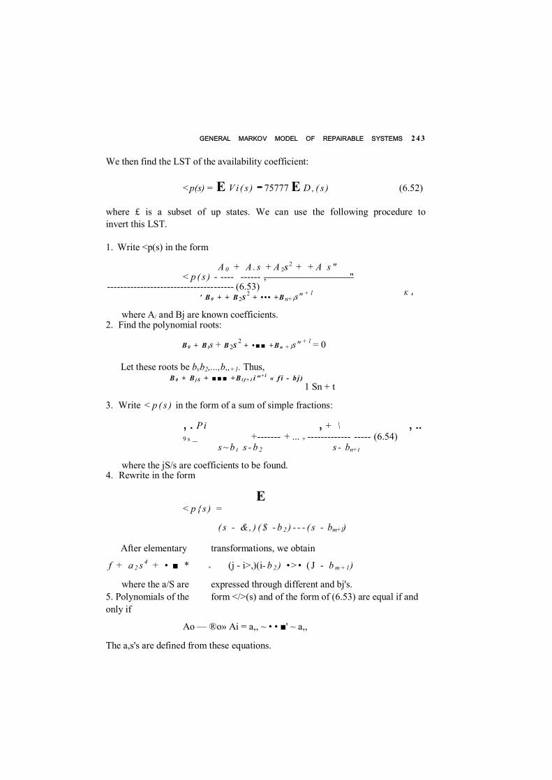
GENERAL MARKOV MODEL OF REPAIRABLE SYSTEMS 2 4 3
We then find the LST of the availability coefficient:
<p(s) = E V i ( s ) - 75777 E D , ( s ) (6.52)
where £ is a subset of up states. We can use the following procedure to invert this LST.
1. Write <p(s) in the form
A 0 + A . s + A 2S 2 + + A s " < p ( s ) - ---- ------ , "
-------------------------------------- (6.53) ' B 0 + + B 2S 2 + • • • + B n+is" + l K '
where A/ and Bj are known coefficients. 2. Find the polynomial roots:
B 0 + B ts + B 2S2 + • ■■ + B n + ls" + l = 0
Let these roots be bvb2,...,b„+1. Thus, B 0 + B j S + ■■■ + B l f + 1 i " + l « f i - b j )
1 Sn + t
3. Write < p ( s ) in the form of a sum of simple fractions:
, . P i , + \ , .. 9 s _ + ------- + ... + ------------- ----- (6.54)
s ~ b t s - b 2 s - bn+t
where the jS/s are coefficients to be found. 4. Rewrite in the form
E < p { s ) =
( s - &, ) ( $ - b 2 ) - - - ( s - bm+l)
After elementary transformations, we obtain
f + a 2 s 4 + • ■ * (j - i>,)(i- b 2 ) • > • ( J - b m + l )
where the a/S are expressed through different and bj's. 5. Polynomials of the form </>(s) and of the form of (6.53) are equal if and only if
Ao — ®o» Ai = a,, ~ • • ■' ~ a,,
The a,s's are defined from these equations.
=

GENERAL MARKOV MODEL OF REPAIRABLE SYSTEMS 2696. After we have found a/s, the inverse LST is applied to < p ( s ) in the form
of (6.54)
f(0- £ ~T ~ K(t) - £ /Hj eb'' \ S j £ n + l 5 + I
REMARK. If a(r) has multiple roots for the denominator, that is, if several b/ s are equal, then (6.54) may be rewritten as
*•>- £ T h V Isisn' ($ ~ b j )
where k is the number of roots equal to b, and n' is the number of different roots. To all terms of the form
Pi (s-fy)*
the corresponding inverse LST is applied:
p. r*~ (M - b f Y '(*-i)!
6.4.3 Probability of Failure-Free Operation To determine the probability of a failure-free operation, absorbing states are introduced into the transition graph. They are the system's failure states. Transitions from any absorbing state are impossible, which means that all transition intensities out of an absorbing state are 0. We can change the domain of summation in the previous equations in a way which is equivalent to eliminating the zero transition rates. Using the previous notation, we can write for an operational state k:
d -RTPK{*) - -P*(0 E AKL + E AIKPI(0 a l j e e ( f c ) i ^ E ( k )
If the transition graph has m operational states, we can construct m differential equations. (In this case the equations are not linearly dependent. Of course, we may use the normalization condition as one of the equations in this new system, excluding any one of the differential equations.) These equations and initial conditions are used to find the probability of a failure- free operation of the system.
,b,t

270 REPAIRABLE SYSTEMS
We again use the LST to find the following system of linear differential equations:
s < p k ( s ) - p k = - < p k ( s ) £ Aki + £ AikVi(s) (6.55) i e e ( k ) i e E ( k )
for all k e E . The solution of this system of equations can be found with the help of the same methodology as before.
6.4.4 Determination of the MTTF and MTBF Recall that
T - f "p ( t ) d t ' n
If <p i s ) is the LST for the probability of failure-free operation of the system, then
re~"Pit)dt J n
Thus, we can find the MTTF (or MTBF) by solving the following system:
-p* = <p*(0) L L Artft(0) ie«{ *) ieEflfc)
for all k e E . Note once more that this system was derived from (6.55) by the substitution of s — 0. To find the MTTF, one sets the initial conditions as PiiO) = I, where i is the subscript of a state in which the system is totally operable. Obviously, pjiO) = 0 for all the other states. To find the MTBF, we set the initial conditions in the form p*i0) - pf where the />*'s in this case are the conditional stationary probabilities of the states i that belong to E * . The latter is a subset of the up states which the process visits first after the system renewal. The conditional stationary probabilities p f ' s can be obtained from the unconditional ones as
P,( 0)
E />,(o)
T =
Pf =
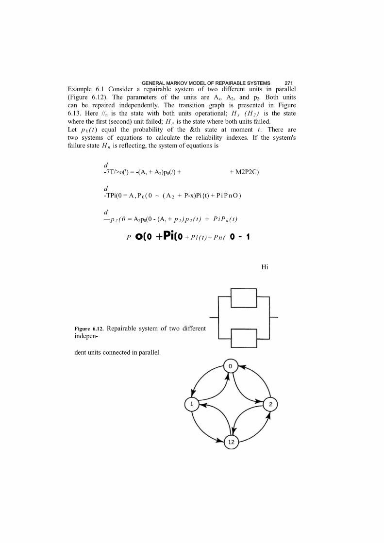
GENERAL MARKOV MODEL OF REPAIRABLE SYSTEMS 271Example 6.1 Consider a repairable system of two different units in parallel (Figure 6.12). The parameters of the units are A,, A2, and p2. Both units can be repaired independently. The transition graph is presented in Figure 6.13. Here //n is the state with both units operational; H x ( H 2 ) is the state where the first (second) unit failed; H n is the state where both units failed. Let p k ( t ) equal the probability of the &th state at moment t . There are two systems of equations to calculate the reliability indexes. If the system's failure state H n is reflecting, the system of equations is
d -7T/>o(') = -(A, + A2)p0(/) + + M2P2C)
d -TPi(0 = A , P 0 ( 0 ~ ( A 2 + P-x)Pi{t) + P i P nO )
d — p 2 ( 0 = A2p0(0 - (A, + p 2 ) p 2 ( t ) + P i P n ( t )
P o(0 +Pi(0 + P i ( t ) + Pn ( 0 - 1
Hi
Figure 6.12. Repairable system of two different indepen-
dent units connected in parallel.
H2

272 REPAIRABLE SYSTEMS
Figure 6.13. Transition graph for the system depicted in Figure 6.12.

GENERAL MARKOV MODEL OF REPAIRABLE SYSTEMS 273
= ~( AI + A 2 >/ 'o ( f ) + M , P ]( t ) + M 2 P 2 O )
= AI P O(0 - ( A2 + M 1) />, ( ')
™P 2(0 = A 2 P 0( R) - ( A , + ^ 2 )p 2 ( t )
~ p 1 2 ( 0 = A 2 p , ( f ) + A ,p 2 ( / )
The corresponding solutions in the form of the Cramer determinants are
1 0
M 2 M O(0)
0 p,(0)
-( A , + f i 2 ) p2(
0)
- ( A , + A 2 ) M i
A , ~ ( A 2 + M j )
A , 0
1 0
-(A, + fi2)
M2
0 - ( A , + m 2 )
If state Hn is absorbing,
T= - M 2
0 + f i 2 )
1 Mi
( A O + M I ) 0
1 ( A , + A 2 )
A ,
J t . 0 ) _ _ .(A,+A2)
A] A ,
Mi - ( A 2 + f L i )
0
1 ~ ( A o + M i )
0
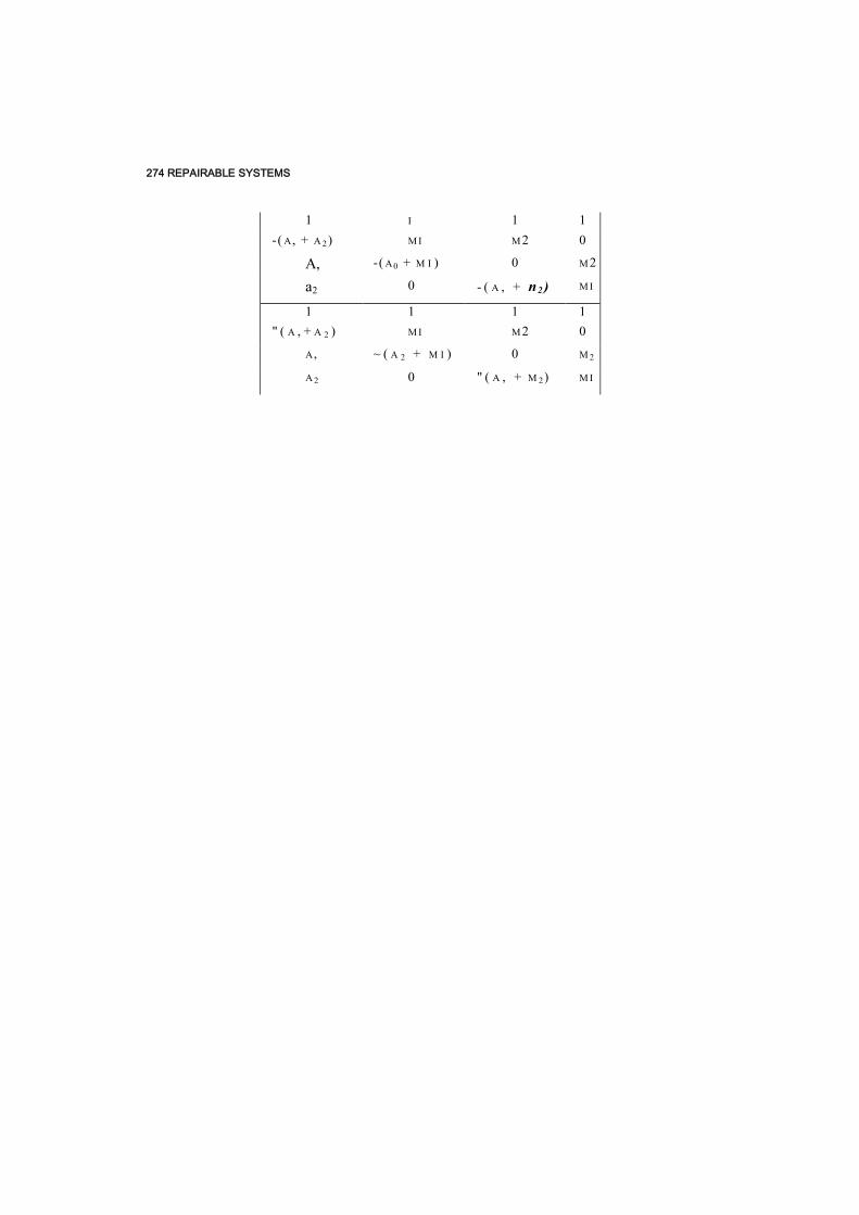
274 REPAIRABLE SYSTEMS
1 I 1 1 -( A , + A 2) M I M 2 0
A, -( A0 + M I ) 0 M 2
a2 0 - ( A , + n2 ) M I
1 1 1 1 " ( A , + A 2 ) M I M 2 0
A , ~ ( A 2 + M I ) 0 M 2
A 2 0 " ( A , + M 2) M I

TIME REDUNDANCY 275
The solutions are not presented in closed form because of their length and complexity.
6.5 TIME REDUNDANCY
Considering reliability indexes, we emphasize that so-called time redundancy might be a very effective measure of a system's reliability improvement. This type of redundancy can be used in two main cases:
• The required time of operation completion by an absolutely reliable system is less than the time admissible for operation performance. • System failures leading to short idle periods might be ignored in the sense of successful operation performance.
These problems are solved with special mathematical methods differing from the usual ones used in other reliability problems. Let us consider several main types of systems with time redundancy.
6.5.1 System with instant Failures Consider a system performing an operation of duration tQ. System failures are very short, practically instantaneous. The flow of these failures can be successfully described by a point renewal process. Each failure interrupts a system's successful operation, and the system is forced to restart its operation from the beginning. In other words, we assume that a failure destroys the result of an operation. For restarting the operation in an attempt to complete the required performance, the system must have a time resource.
Such situations are encountered in practice if one considers a computer operating with short errors which destroy a current result. A computer performs a task which requires t ( ) units of failure-free time for its successful performance. Thus, if there is a time resource, a computer can perform its operation even after the appearance of some error.
We assume that the total time for the system performance is 7 9. Let us also assume thai the system begins to operate at the moment t — 0 when it is "new." The distribution of the TTF is Fit). Let R Q i 6 \ T ) denote the probabil- ity that during interval [0, T] there will be at ieast one period between failures exceeding the required value 0, and let P(f) = 1 — F i t ) .
The system performs its operation successfully during time T if two events occur:
• There are no failures during time interval [0, 0], • A failure has occurred at x < 8 , but, after this moment, the system successfully performs its operation during the remaining time T — x .
The latter event is complex. First, a failure might occur at any moment of time between 0 and 0, and, second, at the moment of a failure the process
276 REPAIRABLE SYSTEMS
starts from the beginning but for a smaller time interval. This verbal explana- tion leads us to the recurrent expression
R 0 ( e \ T ) = P( 9 ) + [ B R 0 ( e \ T - x ) d F{ x ) (6.56) J o
If the remaining interval is smaller than 9, the operation cannot be per- formed successfully. This leads to the condition
R 0 ( 6 \ x < 0 ) = 0
Equations of such a recurrent type are usually solved numerically. We will not provide a mathematical technique for this solution. Above we considered a situation where a system begins to operate at moment t = 0. Now let us assume that a system is in an on-duty regime and a request for starting the operation arrives in a random time. More exactly, we assume that we consider a stationary process, and a random time from the request arrival to a system failure is a residual time. Such a situation is typical of many military systems which must be ready at all times to perform their duties: no enemy in modern times informs you about the beginning of hostile actions. Let the tilde denote a distribution of the residual time. In this case the expression of interest is not changed significantly. We give it without explana- tion because of its obviousness:
/?O(0|T) = P( 0 ) + ( 8 R o ( 0 \ T - x ) d F( x ) (6.57) J o
where the function R 0 under the integral must be taken from (6.56) with the corresponding condition. Of course, in this case we must again write the condition
K(0U < f „ ) = 0
which means that a system cannot successfully perform its operation if the time resource is smaller than the required time of operation.
6.5.2 System with Noninstant Failures
If failures are noninstant, one must take into account the lengths of idle periods between up periods. Let G ( t ) denote a distribution of idle time. If a failure has occurred within the first interval [0, f0], a random period of idle time is needed to restore the system. In general, there are no restrictions on the length of the idle time y . Thus, we must consider the possibility that this value changes within the entire interval [*, T - *]. At the same time, if the system spent x units of time for unsuccessful operation and then y units of

TIME REDUNDANCY 277
time for restoration, only T ~ x — y units of time remain to perform the operation. This verbal description permits us to write a recurrent expression
R ( d \ T ) = P( d ) + C X R ( t 0 \ T - x - y ) d G (y ) J n J q
where Jt(0U < t 0 ) = 0. Now we consider the above-analyzed system which is operating in an on-duty regime. In principle, the explanation of the equation remains similar to the previous case. We must additionally take into account the fact that the system at an arbitrary stationary moment of time can be found in one of two possible states: up or down. We only explain the situation where a system at the beginning of operation is in a down state. In this case one first observes a residual restoration time and after this a system is considered as "new." Again, we use a tilde to denote the distribution of a residual value. The expression for this case can be written in the form
R ( t 0 \ T ) = K P( 0 ) + f [ ~ x R { t 0 \ T - x ~ y ) d G {y ) J o L-'o
+ k ( ' R (e \ T - x ) d G (x ) ' n
where K is the availability coefficient and k = 1 - K . Recall that K = t / ( T + r) where T is the MTTF and r is the MTR.
6.5.3 System with a Time Accumulation Some systems must accumulate time of successful operation during a total period of performance. Of course, in this case we consider an alternating process of up and down periods. Denote the probability that a system will accumulate more than 6 units of successful operation during period T as S(0|r). For this probability one can consider two events that lead to success:
• A system works without failures during time from the beginning. * A system failed at moment x < 6 , was repaired during time y , and during the remaining interval of T — x — y tries to accumulate 6 — x units of time of successful operation. This description leads us to the recurrent expression
S ( d \ T ) = P( 0 ) + f 0 f r X S ( t 0 - x l T - x - y ) d G ( y ) J o l/o
d F( x ) (6.58)
d F( x )
d F( x )
278 REPAIRABLE SYSTEMS
This expression is correct for the case where a system starts to perform at t = 0.
If a system is in an on-duty regime and begins to accumulate time of successful operation at a stationary arbitrary moment, one must take into account that a system may occur at an up or down state. Each of the corresponding periods is represented by a residual time. The expression for the probability that a system will accumulate more than 6 units of successful operation during period T as S(0|7") starts to perform at an arbitrary moment is
S ( 0 \ T ) = K P( 6 ) + f T * S { 0 - x \ T - x - y ) d G ( y )
Jo l/o
+ k [ ' R { 0 \ T~ y ) d G( y ) J n
where F ( x ) = 1 — P( x ) is the distribution of a time of failure-free operation, G(x) is the distribution of a repair time, and S(0|7 - Jt) is taken from (6.58). Expression (6.59) is correct with the additional condition S(jc|y < *) = 0.
6.5.4 System with Admissible Down Time A system is considered to be successfully operating if during period T there will be no down time larger than T J . This case in some sense is a "mirror" for that considered on page 249. We will omit the details and write the recurrent expression immediately:
Q { v \ T ) = P( T ) + f 7 \ ( V Q ( V \ T - x - y ) d G ( y ) J o l/o
This expression is correct under an additional condition:
Q ( v \ x ^ v ) = 1
The same system may be considered in an on-duty regime. We again will omit the details and write the recurrent expression
P( T) + [ f Q ( V \ T - x ~ y ) d G (y ) A) l/o
+ k f V Q ( V \ T - y ) d G ( y ) Q ( v \ T ) - K
d F( x )
(6.59)
d F( x )
d F( x)
TIME REDUNDANCY 279 This expression is correct under an additional condition:
Q ( v \ x < r , ) = 1
This subject as a whole requires a much more detailed discussion. There are many interesting detailed models concerning, for instance, computer systems. The reader who is interested in the subject can refer to Kredentser (1978), Cherkesov (1974), and Ushakov (1985, 1994). Some applications of these methods to oil and gas transportation systems can be found in Rudenko and Ushakov (1989).
CONCLUSION
The models of repairable systems discussed in this chapter concern some ideal schemes: switches are supposed to be absolutely reliable; monitoring of the operation of the system's units is continuous; after repair, units are considered to be as good as new; and so forth. Besides, when using Markov models, one must assume that all distributions of failure-free intervals and repair times are exponentially distributed.
All of these assumptions seem to make such kinds of models practically useless. But the same can be said about any mathematical model: a mathe- matical model is only a reflection of a real object or real process. Each mathematical model may only be used if the researcher understands all of the model's limitations.
First of all, Markov models are very simple though simplicity is not a good excuse for their use. But using Markov models for highly reliable systems very often gives the desired practical results in reliability prediction.
Next, the lack of some realistic assumptions concerning switching and monitoring may be taken into account. (We try to show this in the next chapter.) This point is really very serious and must be taken into considera- tion. To demonstrate the importance of continuous monitoring of redundant units, let us consider a simple example.
A repairable system consists of n units in parallel (i.e., this is a group of one main and n — 1 loaded redundant units). A system unit has an exponen- tially distributed TTF. Redundant units are checked only at the moment of failure of the main operating unit. At this moment all failed units are repaired instantaneously! If there is at least one nonfailed redundant unit, this unit replaces a failed main unit and the system continues to operate under its initial conditions. It seems that such a system with instant repair should be very reliable. But this system has no control over the system's unit states.
Find the MTTF of this system on the basis of simple explanations. A main unit has failed, on average, in T units of time, and with probability \ / n up to this moment all of the remaining n - 1 units have failed. It is clear that such

280 REPAIRABLE SYSTEMS a system will work, on average, nT units of time until a failure. But as the reader will recall, a standby redundant group of n units without repair has the same MTTF!
It is difficult to find out who wrote the pioneering works in this area. The reader can find a review in the next chapter dedicated to renewal duplicated systems—a particular case of redundancy with repair. The reader can find general information on this question in a number of books on reliability, some of which are listed at the end of this book. For a brief review, we refer the reader to the Handbook of Reliability Engineering by Ushakov (1994).
Time redundancy represents a separate branch of renewal systems, closely related to the theory of inventory systems with continuous time. The reader can find many interesting models for reliability analysis of such systems in Cherkesov (1974) and Kredentser (1978). The reader can find applications of these methods to gas and oil pipelines with intermediate storage in Rudenko and Ushakov (1989). General methods of time redundancy are briefly pre- sented in Ushakov (1985, 1994). An interesting discussion on repairable systems can be found in Ascher and Feingold (1984).
REFERENCES
Ascher, H., and H. Feingold (1984). Repairable System's Reliability: Modelling, Infer- ence, Misconceptions and Their Causes. New York: Marcel Dekker.
Cherkesov, G. N. (1974). Reliability of Technical Systems with Time Redundancy. Sovietskoe Radio: Moscow.
Gertsbakh, I. B. (1984). Asymptotic methods in reliability theory: a review. Adv. in Appl. Probab., vol 16.
Gnedenko, B. V., Yu. K. Belyaev, and A. D. Solovyev (1969). Mathematical Methods of Reliability Theory. New York: Academic.
Gnedenko, D. B., and A. D. Solovyev (1974). A general model for standby with renewal. Engrg. Cybernet. (USA), vol. 12, no. 6.
Gnedenko, D. B., and A. D. Solovyev (1975). Estimation of the reliability of complex renewable systems. Engrg. Cybernet. (USA), vol. 13, no. 3.
Kredentser, B. P. (1978). Prediction of Reliability of Systems with Time Redundancy (in Russian). Kiev: Naukova Dumka.
Rudenko, Yu. N., and I. A. Ushakov (1989). Reliability of Energy Systems (in Russian). Novosibirsk: Nauka.
Solovyev, A. D. (1972). Asymptotic distribution of the moment of first crossing of a high level by birth and death process. Proc. Sixth Berkeley Symp. Math. Statist. Probab., Issue 3.
Ushakov, 1. A., ed. (1985). Reliability of Technical Systems: Handbook (in Russian). Moscow: Radio i Sviaz.
Ushakov, I. A., ed. (1994). Handbook of Reliability Engineering. New York: Wiley.

EXERCISES
6 .1 A system has an exponentially distributed TTF with a mean t - 100 hours and a repair time having a general distribution G ( t ) with a mean r = 0.5 hour. Find the system's stationary interval availability coefficient for the operation during 0.5 hour.
6 .2 Construct a transition graph for a repairable system consisting of two main units, one loaded redundant unit which can replace instanta- neously each of them, and three spare units. After a main unit has failed, a loaded redundant unit replaces it. In turn, one of the spare units replaces the redundant unit. Failed units are subjected to repair after which they become as good as new. All units are identical, each with a failure rate equal to A. There are two repair facilities, each of which can repair only one failed unit at a time. The intensity of repair by a repair facility is equal to fi. After a total exhaustion of all redundant units, repair is performed over the entire system with inten- sity M .
6 .3 Construct a transition graph for the system depicted in Figure E6.2.
Figure E6.2. Structure diagram for the sys- tem described in Exercise 6.3.
SOLUTIONS
6 .1 The stationary availability coefficient depends only on the mean and not on the type of distribution of the TTF and repair time. Thus, K = (100)/(100 + 0.5) = 0.995. If the system is found within a failure-free interval, which is exponentially distributed, then the probability of successful operation of length f0 beginning at an arbitrary moment of time can be written as
lim P ( t , t + t 0 ) =e~">/T l — oo
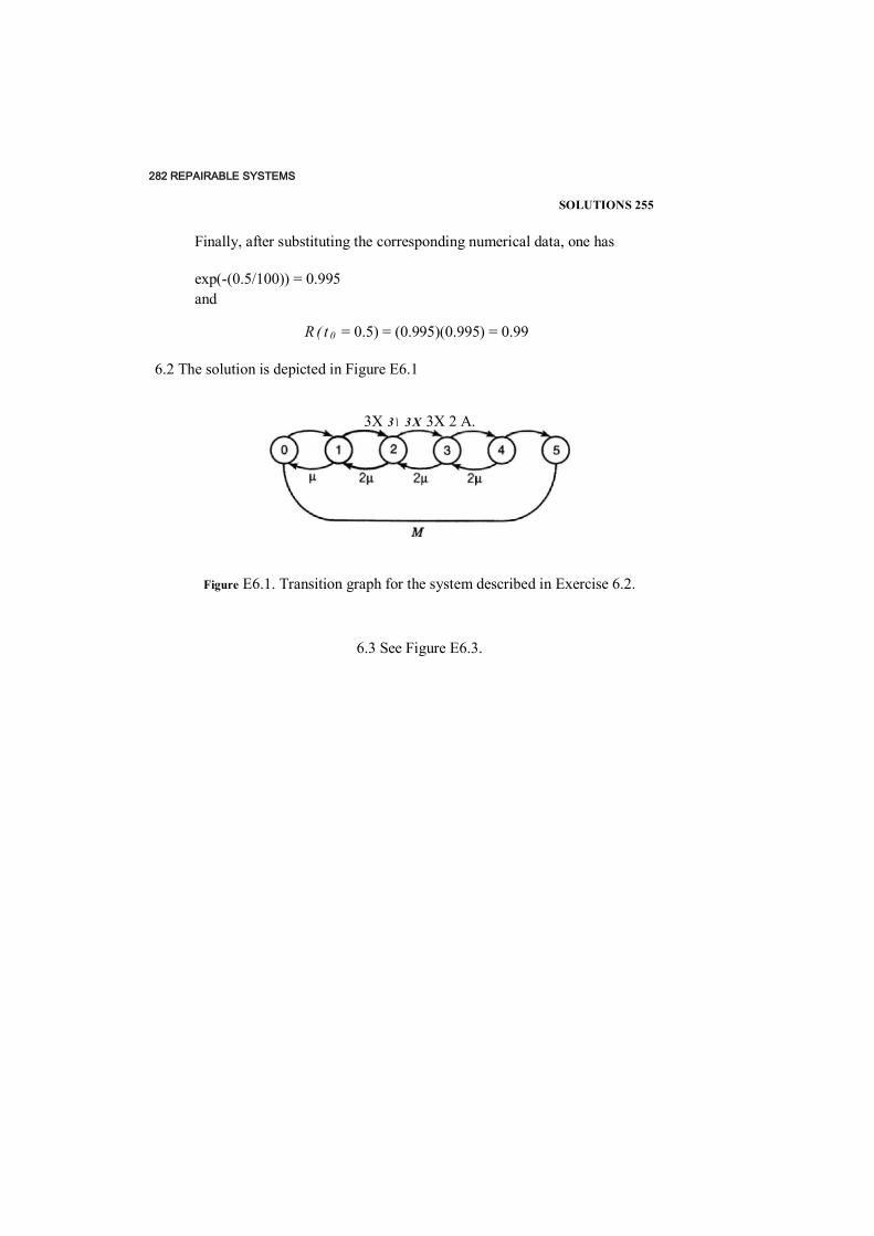
282 REPAIRABLE SYSTEMS
SOLUTIONS 255
Finally, after substituting the corresponding numerical data, one has
exp(-(0.5/100)) = 0.995 and
R ( t 0 = 0.5) = (0.995)(0.995) = 0.99
6.2 The solution is depicted in Figure E6.1
3X 3 \ 3 X 3X 2 A.
Figure E6.1. Transition graph for the system described in Exercise 6.2.
6.3 See Figure E6.3.

Figure E6.3. Transition graph for the system described in Exercise 6.3.
CHAPTER 7
REPAIRABLE DUPLICATED SYSTEM
Duplication refers to the particular case of redundancy where there is a single redundant unit to support a single working (main) unit. We distinguish this particular case for both practical and methodological reasons. First of all, when a designer feels that the reliability of some unit is low (sometimes this understanding may occur on a purely intuitive level), duplication is a simple way to improve it. Indeed, if a failure may occur with a relatively small probability, it is generally not necessary to have more than one redundant unit. In general, the number of redundant units depends on the desired value of the system's reliability index and/or on permissible economical expendi- tures.
From a methodological viewpoint, duplication presents the clearest way to explain certain special mathematical tools, their idiosyncrasies, and their ability to treat a real technical problem. It allows for the possibility of following mathematical transformations in detail. (Unfortunately, nobody has either the capacity or the desire to present similar detailed explanations for more complicated cases.)
7.1 MARKOV MODEL
As we have pointed out, a duplicated renewal system is one of the most frequently encountered structures in engineering practice. In the reliability analysis of electronic equipment (at least, in the first stages of design), the distributions of the time to failure and of the repair time arc usually assumed exponential. In this case Markov models are adequate mathematical models 256
Probabilistic Reliability Engineering. Boris Gnedenko and Igor Ushakov

MARKOV MODEL 285 to describe such systems. We note that the final results obtained with Markov models are usually acceptable in a wide variety of practical cases (especially when applied to highly reliable systems).
7.1.1 Description of the Model Consider a duplicated system consisting of two identical units. Usually, the following assumptions are made:
• The system units are mutually independent. • After a failure of the operating unit, its functions are immediately
assumed to be performed by the redundant unit. • Repair (renewal) of a failed unit begins immediately. • A repaired unit is considered to be a new unit. • The switching device is considered absolutely reliable.
Two important aspects of a renewal system should also be taken into account: the regime of the redundant unit and the attributes of the repair workshop.
The following regimes of a redundant unit characterized by failure rate A' might be considered:
1. The redundant unit operates under the same conditions as an opera- tional unit; that is, their failure rates are equal, A = A'.
2. The redundant unit is in a completely idle state, that is Ar = 0. 3. The redundant unit is in an intermediate state between completely idle
and operational, that is, 0 < A' < A.
The first case is often referred to as internal redundancy, the second as standby redundancy, and the third as waiting redundancy.
The renewal regime might be distinguished by the number of repair facilities (places for repair, the number of technicians special equipment), that is, by the number of failed units which can be repaired simultaneously. We consider two cases:
1. An unrestricted renewal when the number of repair facilities equals the number of possible failed units (in this particular case, two facilities are enough).
2. An extremely restricted renewal with a single repair facility.
The transition graphs describing these models are presented in Figure 7.1 (there are two of them: with and without an absorbing state). Corresponding particular cases for different regimes of redundant units and different at- tributes of the repair shop are reflected in Figure 7.2.

286 REPAIRABLE DUPLICATED SYSTEM
Figure 7.1. Transition graph for a renewable dupli- cated system: («) state 2 is reflecting; ( b ) state 2 is absorbing.
© © n>j 1 n f1!
L0 0 ir v
© o O p
© © (a)
Figure 7.2, Transition graphs for four main models of a renewable duplicated system: (a) a loaded redundant unit, two repair facilities; (fc) a loaded redundant unit, one repair facility; (c) an unloaded redundant unit (spare unit), two repair facilities; (d) an unloaded redundant unit, one repair facility.
Using the above-described technique, corresponding systems of equations for obtaining the various reliability indexes can be easily written. In this particular simple case, the solutions can be obtained in a general form. The final results for particular cases can be derived easily.
7.1.2 Nonstationary Availability Coefficient The system of differential equations (in canonical form) with the initial conditions Pa(0) = 0 is
d ■ p 0 ( O = ~ x 0 P Q ( t ) dt
-/>,(() - A0i>0(f) - (A, + p l ) P i ( t ) + ( * 2 P 2 ( t )
i = / > 0 ( 0 + ^ . ( 0 + ^ ( 0 P0( 0) = 1
(b)
© X"
a i k
VL ©
© 0 ©
Q r i t t
2T'
Q, \ v
© ©
Xw
© ©
(7.1)
MARKOV MODEL 287
The LST of (7,1) is
(A0 + j)<p0(j) -Mi<Pi(s) - 1 - A0<p„(s) + (5 + A, + Mi)<Pi(-0 + H 2<P2(s) = 0
s<Po(s) + 5<p,(s) + s<PzO) = 1
Notice that the availability coefficient equals
*<o = n c ) + ^ ( 0 = 1 - ^ ( 0
Thus, to find the LST of K i t ) , we can find [see the last line in (7.2)]
I <P(i(s) + <Pi(s) = j ~
From (7.2) it is easy to write
+ f t i + s 0
+ S(A0 + Ai + Mi + f t 2 ) + AoAi + a
OM2 + M1M2]
Thus,
+ fit-1) = 7 ~ ( f 2 ( s ) - g 2 + + A ' + + ^ + A q M z + s[i2 + s(A0 + A, + /a, + fi2) + A0A[ + A + /i,/i2]
Now we should refer to the technique described in Chapter 6 in the section on Markov processes:
1. Represent the LST as the sum of simple fractions
j2 + i(A„ + A( + /it + n2) + A oM 2 + M1A2 s[53 + s( A0 + A( + ju,, + + A0At + \0n2 +
A B C 5 — 5 - 1
where A , B , and C are unknown.
(7.2)
A0 + s — A„
0
~ti 2 S A()A,
A0 + 5 "An
-Ml A] + + s
s
s — s ,

288 REPAIRABLE DUPLICATED SYSTEM
2. Find the roots of the denominator. The first two roots of the denomina- tor are conjugate, that is
where, in turn,
a = A0 + A, + fjLx +
P = A 0 A l + A 0 M 2 + M l / ^ 2
and s 3 = 0. 3. Find the unknown values A , B , and C by equalizing the polynomial
coefficients of the numerators. 4. Apply the inverse LST to obtain simple fractions with the numerators
A , B , and C found above to obtain the final result.
After these transformations the result is obtained
A0A,
K ( 0 = 1 - s i s->
Obviously, if s, = s 2 , I'Hospital's rule must be used.
Now any result of interest can be obtained by substituting the appropriate values of A and /i. In general, the solution for a duplicate renewal system can be obtained in a closed form, but this solution is not very compact, even for the simplest case.
Of course, we should notice that, for active redundancy and unrestricted repair, the final result can be written immediately with the use of the appropriate result for a single unit:
^ ( 0 = ! - ( ! - K *( f ) ) = 1 -
where K * ( t ) is the nonstationary availability coefficient of a single unit. This result is obvious because both units are supposed to be mutually indepen- dent.
7.1.3 Stationary Availability Coefficient The solution can be derived from (7.1) by putting the derivatives equal to 0. The same result can be directly obtained from the corresponding transition
(7.3)
J iJ'-
.-(A+pOM( I"
A + JLA
MARKOV MODEL 289
graph by writing the equilibrium equations:
~\0PQ + - 0
Aq/q - (A, -Jtt,)?! + /*2P2 = 0
+ + P 1 = 9
The solution is
9 +
(7.4)

290 REPAIRABLE DUPLICATED SYSTEM
« Mi
A0 -(A 0
1 1 1 -A, A 0 - ( A t + M i ) M 2
1 1 1
1 aoM2 + M1M2
To obtain values of this reliability index for different cases, the specific A's and /A 'S should be substituted. The results for the four most important cases depicted in Figure 7.2 arc presented in Table 7.1. In this table we used the notation y = For highly reliable systems with A « I, all of the expres- sions in Table 7.1 can be easily transformed to obtain the approximations given in Table 7.2. The expressions in Table 7.2 allow one to give an understandable explanation of all of the effects. Naturally, the worst value of K gives the case of active redundancy and restricted repair (the failure rate
TABLE 7.1 Availability Coefficient for Four Main Models of a Renewable Duplicated System
(a) (b) 1 1
, v 1 + ----------------------- ---- T— 1 +
1 + 2y 1 + 4y
1 1 y1 y2
1 + — --------------r 1 + 2(1 + y ) 1 + y
(A) Loaded redundant unit; (B) unloaded redundant unit; (a) two repair facilities; (b) one repair facility.
0-A
A n AK = 1 - P 2
i = 1 ~ = 1 - 0 A0A, + A0^2 + M1M2Mi
(7.5)A 0 A t
A0M2 + M1M2
(A)
(B)

MARKOV MODEL 291
A0 is the largest and the repair rate p2 is the smallest). The case of unrestricted repair yields a mean repair time of less than one-half of the restricted repair time (1/2/a and \/fi, respectively). Below in this section we will show that the MTTF of highly reliable systems of active redundancy is one-half of the MTBF for standby redundancy. Of course, for two independent units, that is, when the redundancy is active and the repair is unrestricted, we can write
K = i - ( i - K * y = i -
using the availability coefficient for the single unit
K * . Then
2A + n2 1 1
A2 + 2A + \j}
The intermediate case with either the "underloaded" redundant unit (when A < A() < 2A) or with the "dependent" repair when (/a < p2 < can be easily obtained numerically from the general expression (7.5). Of course, this index can be realized as
lim K ( t ) t
but this is not effective when K i t ) is not available.
7.1.4 Probability of Failure-Free Operation
TABLE 7.2 Approximation lor Availability Coefficient for Highly Reliable Duplicated System
(a) (b) (A) 1 + 2 y 1 + 4-y
v 2 y 2 (B) 1 Y
2(1 + y ) 1 7
1
(A) Loaded redundant unit; (B) unloaded redundant unit; (a) two repair facilities; (b) one repair facility.
A + p
1 + 1 +
1 + 2 y2A + M2

292 REPAIRABLE DUPLICATED SYSTEM
To find this probability, it is necessary to construct a system of differential equations using the graph of Figure 7.1b with absorbing state 2. In this case the equations are not linearly dependent. For the initial conditions P0iO) = 1,

MARKOV MODEL 293
the system of linear differential equations is
- p 0 ( O = - \ 0 P 0 ( t )
/> , ( ' ) =A 0 /> 0 (0 - ( A, + f i l ) P 1 ( t )
PO (0 ) = 1
The LST of (7.6) is
(A 0 + s ) ( p 0 ( s ) - = 1
- A 0 < p 0 ( s ) + (A, + M i + s ) ( p , ( s ) =» 0
and the solution has the form
— A 0 A, + M i + s
s + A 0 4 - A, + M i
s 2 + s (A 0 + A, + M i) + A 0 A,
Applying the procedure that we used to obtain (7.3), we find
1
(s?ef*' — s2es1') r* - t* J , S 2
where the superscript (0) stands for the initial conditions Po(0) = 1 and also
<«*r -P
a * = A 0 + A[ + M i
(3* = A 0 A,
If we are interested in the system's PFFO immediately after its repair, it is necessary to set P,(0) — 1. The corresponding system of linear algebraic equations in the LST is
(7 .6 )d t
(7 .7 )
1 "M i A 0 1
0 A, + M i + s -A 0 0
A 0 + s "M i
<Po(s) + =
(7.8)
p«»(0 = (7-9)
a

294 REPAIRABLE DUPLICATED SYSTEM
(A 0 + s )< p 0 ( s ) - M i<P i( s ) = 0
- Ao <P o (^) + ( A i + M i + s ) ( p i ( s ) = 1
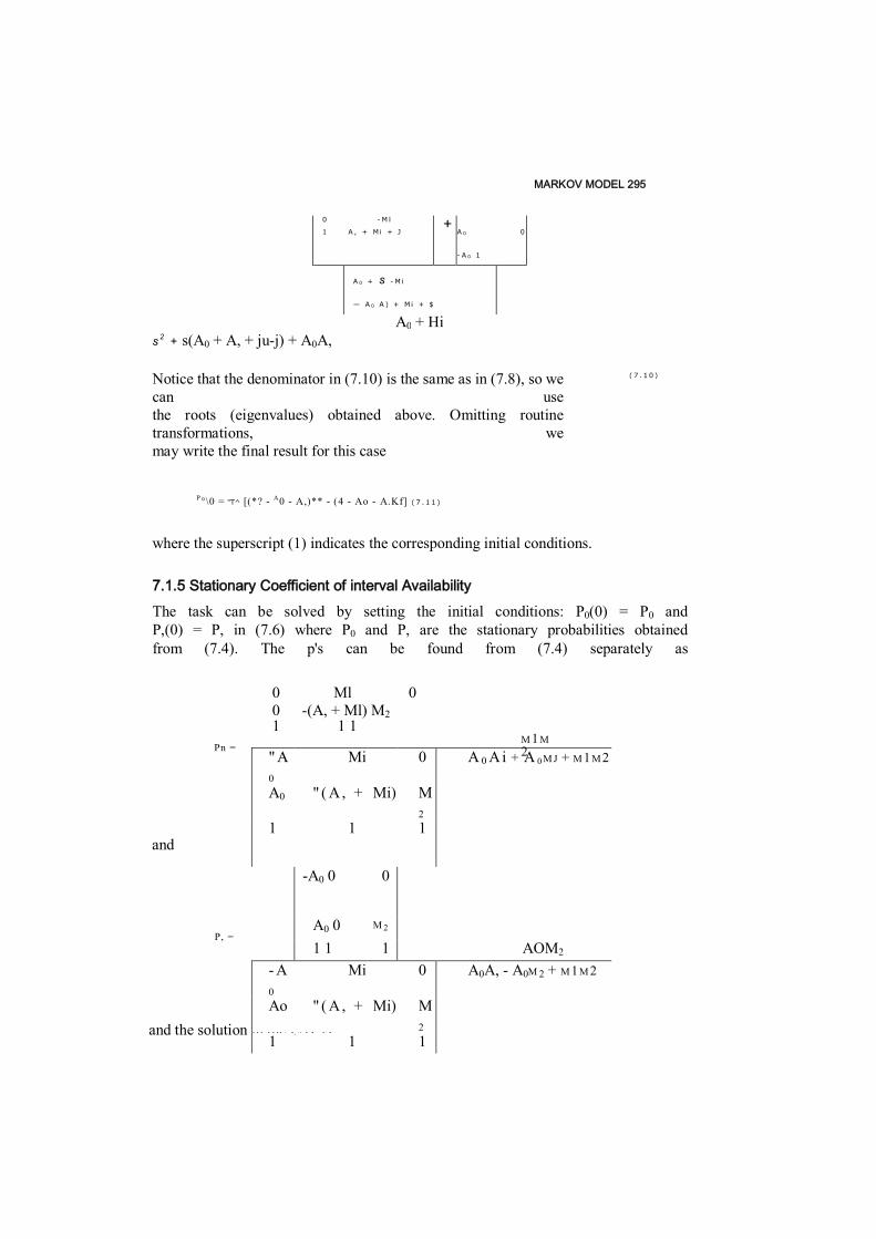
MARKOV MODEL 295
s 2 + s(A0 + A, + ju-j) + A0A,
Notice that the denominator in (7.10) is the same as in (7.8), so we can use the roots (eigenvalues) obtained above. Omitting routine transformations, we may write the final result for this case
P°\0 = "T^ [(*? - A0 - A,)** - (4 - Ao - A.Kf] ( 7 . 1 1 )
where the superscript (1) indicates the corresponding initial conditions.
7.1.5 Stationary Coefficient of interval Availability The task can be solved by setting the initial conditions: P0(0) = P0 and P,(0) = P, in (7.6) where P0 and P, are the stationary probabilities obtained from (7.4). The p's can be found from (7.4) separately as
0 - M l
1 A , + M i + J +
A 0 0
- A 0 1
A 0 + s - M i
— A 0 A ) + M i + $
A0 + Hi
( 7 . 1 0 )
and the solution in the LST is
" A0
Mi 0 A 0 Ai + A 0 M J + M 1M 2
A0 " ( A, + Mi) M2
1 1 1
-A0 0 0
A0 0 M 2
1 1 1 AOM2 - A0
Mi 0 A0A, - A0M 2 + M 1M 2
Ao " ( A, + Mi) M2
1 1 1
0 Ml 0 0 -(A, + Ml) M2 1 1 1
M 1M2 Pn =
and
P, =
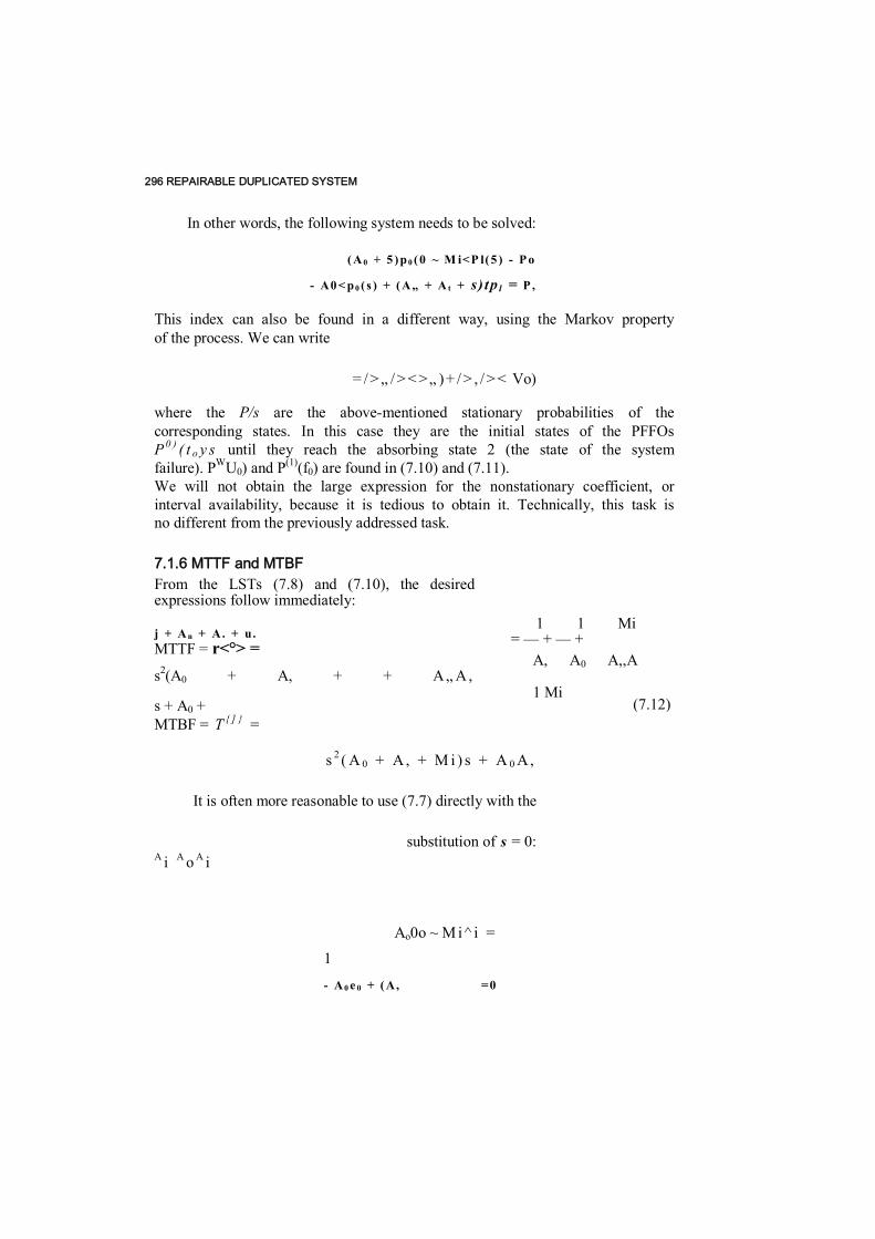
296 REPAIRABLE DUPLICATED SYSTEM
In other words, the following system needs to be solved:
(A 0 + 5 )p 0 (0 ~ M i<P l(5 ) - P o
- A0 < p 0 ( s ) + (A„ + A t + s) tp l = P ,
This index can also be found in a different way, using the Markov property of the process. We can write
= / > „ / > < >„ )+ / > , / > < Vo)
where the P/s are the above-mentioned stationary probabilities of the corresponding states. In this case they are the initial states of the PFFOs P 0 ) ( t o y s until they reach the absorbing state 2 (the state of the system failure). PWU0) and P(1)(f0) are found in (7.10) and (7.11). We will not obtain the large expression for the nonstationary coefficient, or interval availability, because it is tedious to obtain it. Technically, this task is no different from the previously addressed task.
7.1.6 MTTF and MTBF From the LSTs (7.8) and (7.10), the desired expressions follow immediately:
j + A n + A. + u. MTTF = r<°> = s2(A0 + A, + + A„ A,
s + A0 + MTBF = T { ] } =
s 2 ( A 0 + A , + M i ) s + A 0 A,
It is often more reasonable to use (7.7) directly with the
substitution of s = 0: A i A o A i
Ao0o ~ M i ^ i =
1
- A 0 e 0 + (A, =0
1 1 Mi = — + — +
A, A0 A,,A
1 Mi (7.12)
MARKOV MODEL 297
where 0, and d2 are values such that the MTTF = 0, + 02. The solution of this equation system yields
1 A , + M i 1 M i
0 n = — and 0 , = — - - - - - - - - - - - - - — + A[ 1 A 0 A, A 0 A 0 A j
Of course, this result coincides with (7.12). The MTBF may be computed in the same manner, and we leave this as an exercise.

298 REPAIRABLE DUPLICATED SYSTEM
To find the system's MTTF, it is sometimes more convenient to use the following arguments. Consider the transition graph in Figure 7.1. Let us find the system's MTTF (this means that at / = 0 the system is in state 0). Denote the mean time needed to reach the absorbing state 2 from the initial state 0 as T()2 and from state 1 as T(Apropos, T02 = MTTF and T„ « MTBF.) Obviously,
T02 - ~ + Tu (7.13) Aft
because the process inevitably moves from state 0 to state 1, After this, based on the Markov property, the process can be considered to be starting from state 1. The process stays in state 1 for an average time 1/(A2 + ft,) and then moves either to state 2 or to state 0, It moves to state 0 with probability /i)(A2 + ^j) and then starts traveling again from state 0. Hence, we can write
T\Z = V ( A Z + + O I 7 O 2 > / ( A 2 + P I )
Substituting (7.14) into (7.13) yields
MTTF - T02 =
A, + M - i
= — + 1 + /i| A 0 A ! Ag A,
From (7.13) it also immediately follows that
1 P i MTBF = ri2 = — +
Now, on a very understandable and almost verbal level, we can explain the difference between the MTBF (or the MTTF) for repaired duplicated sys- tems of identical units which have a different regime for the redundant unit. For active redundancy Au = 2A and for standby redundancy A0 = A. In other words, in the first case, the system stays in state 0, on average, one-half the time that it stays in the second case. This fact can be seen more clearly from
(7.14)
1 1 +
A 0 + A , + ft tMi A 0 A,+ / i , A 0 A,

DUPLICATION WITH AN ARBITRARY REPAIR TIME 299
the approximate expressions for a highly reliable system when y = A//x <K 1:
MTTFactive = 7 + ™ + ^ (7-15)
and
MTTF—.' I+ X + 7 - £ (7J6)
Incidentally, (7.15) and (7.16) could be explained on the basis of the Renyi theorem. Consider an alternative renewal process describing the operation of a repaired duplicated system. For a highly reliable system, this process can be approximately represented as a simple renewal process if one neglects small intervals of being at state 1. The system's successful operation period consists of the sum of a random number of intervals of the length 1/A0 until the process has jumped to state 2. This random number has a geometrical distribution with parameter p = Mi/(At + Mi) ~ 1 ~ T- Thus, the sum also has an exponential distribution with parameter A()y. This means that approximately
/,0('«)=/,°(^)-EXP(-A0Y/0) (7.17)
We should now remember that for active redundancy Ay = 2A and for standby redundancy A0 = A. We wrote all of these solutions in such a detailed form because the LST technique is very important in engineering applications. A certain amount of practice is needed to apply this to practical problem solutions. We believe that the best way to master these approaches is to work out simple exercises.
7.2 DUPLICATION WITH AN ARBITRARY REPAIR TIME
For repairable duplicated systems, models more complicated than the Markovian type can be analyzed. We first consider a model described in the following way:
10 Both units are independent and identical. * The operating unit has an exponential distribution of time to failure F(r)
with parameter A, and the redundant unit has a similar distribution F,(r), also exponential with parameter A,, 0 < A( < A. (This condition means that the redundant unit might be, in general, in an underloaded regime.)
I 1 i x 1 A + 2A 4 10" 2yA
300 REPAIRABLE DUPLICATED SYSTEM
* The repair time of a failed unit has an arbitrary distribution G i t ) . ' The repair of a failed unit begins immediately after a failure has
occurred. * After repair, the unit becomes completely new. * The repaired unit is immediately installed into the system.
It is clear that after an operational unit has failed, the redundant unit replaces it and becomes operational. A system failure occurs if and only if the operating unit fails during the repair of the other unit, that is, when both of the system's units have failed.
Let us find the distribution of the system's time to failure Rsit). A failure-free operation of the duplicated system during a time period t can be represented as the union of the following mutually disjoint events:
1. The first failure in the system occurs after moment what happens with the redundant unit does not play any role. The probability of this event is exp[( —A -I- A,)/].
2. The first failure of either of the two units occurs at some moment z < t , the failed unit is not repaired during the interval (t - z ) , but the unit in the operating position has not failed up to t . The pro- bability of this event is
T(A + A,)e-(A+A')z[l - G ( t - z ) ] e ~ * ' ~ z ) d z Jn
3. The last event is the most complicated. In this case, as some moment x < t , the duplicated system comes to the initial state, that is, state 0, where both system's units are operational. This occurs if one of the units has failed during the interval [ z , z + d z ], the repair has taken time x - z, and the operating unit has not failed during repair. After the completion of the repair, the system operates successfully during the remaining period of time (t - x) with probability Rit — x) => 1 — Fsit - x ) . The probability of this event is
f ° ° R ( t - x ) dx [ \ \ + - z ) d z J n J n
where g i t ) is the density function of the distribution G i t ) .
DUPLICATION WITH AN ARBITRARY REPAIR TIME 301
Now it is easy to write the final equation for the probability of a system's failure-free operation:
R(t) = «-<*+*■>' + e ~ A ' ( \ + A,) f'e~x»x[ 1 - G( t - * ) ] d x
+ f'R(t - x)e~*'(\ + Aj) dx f X e ~ x < * g ( x - z ) d z (7.18) J o J o
Thus, we have an integral equation with a kernel of the type
R ( t ) — A ( t ) + f ' R ( t - x ) B (x ) d x (7.19) A)
where, in the above case,
A ( t ) = + + A,) jVA'*[ 1 - G { t - * ) ] d x
° (7.20) B ( t ) = <rA'(A + A,) ['e-Azg(t - z) dz
The recurrent equation (7.18) can be solved by the method of sequential iterations. Hut we prefer to obtain the solution in the form of the LST as it allows us to investigate the asymptotical behavior of R ( t ) . If we denote
a { s ) = r e ~ s ' A ( t ) d t J o
b ( s) = f% - "B ( t ) d t J o
<P(j) = re~*'dG(t) J o
< p ( s ) = f e - "R ( t ) d t o
then the solution can be represented in the form
= + <p(s)fc(5) (7.21)
and, finally, the LST of interest is
a ( s )
302 REPAIRABLE DUPLICATED SYSTEM
The functions a(s) and b ( s ) can easily be found from (7.20)
5 + A + (A + A,)[l - i p ( s + A)] (s + A + A.){i + A)
(7.23)
b ( s ) = - - - - - - - - - - - - - - - - - - v ' A + A[ + s
Thus, after substituting (7.23) into (7.22), we obtain
5 + A + (A + A,)[l - ^(J + A)] = ( i + A ) [ i + ( A + A , ) ( l - ^ ( A + f ) ) ] ( 7 ' 2 4 )
Therefore, the general case has been investigated. It is clear that for active redundancy, when A, = A,
5 + A + 2A[I - ¥(A + J)] = (A + s ) [ s + 2A(1 - ¥(A +j))]
For standby redundancy, when At = 0,
s + A + A[l — ^(A +5)]
^ = (A + s ) [ s + A(1-¥(A +j))]
Since (7.24) is the LST of R ( t ) = 1 - F s ( t ) , the MTTF can be derived from this expression directly with the substitution 5 = 0:
r -/ M A + (A +A,)[1 -^(A)] 1 1 T s = ¥>(5)1,,o = -7T , rrr;—„„ = - +
A(A +A,)[1 -*(A)] A (A+ ^[1 "*(*)] (7.25)
In deriving the latter expression, we use the memoryless property of the exponential distribution: if an object with an exponentially distributed ran- dom TTF has not failed until some moment t , then the conditional probabil- ity of the random residual TTF of the object is the same exponential distribution as the original one. Thus, the process of an operation of a duplicated system has the so-called renewal moments, that is, such Markov moments at which all of the prehistory of the process has no influence on the future development of the process starting from this moment.

DUPLICATION WITH AN ARBITRARY REPAIR TIME 303
The MTTF of the duplicated system without repair, as it was obtained above, equals
1 1 T - - - - - - - + -
A + A, A
From (7.25) it follows that the effectiveness of redundancy with renewal increases very quickly as i/r(A) -> 1. Notice that 0(A) is not more than the probability that the random TTF of a unit exceeds the duration of its repair. It means that
a = 1 - < K \ ) = Pr U < V ) - f [ l ~ e ~ k , ] d G { t ) J f \
is the probability of an unsuccessful repair, denoted by a. Here £ is a random TTF and 77 is a random repair time. Notice that for the exponential distribution this probability equals A/(A + p.) = y/(l + y) where y = A/^t. Let us make a final remark concerning the system MTTF. It is possible to write a clear and understandable recurrent equation to express T . The period of a system's successful operation can be represented by a sequence of cycles of the type "time to failure of any of the system's units + time of successful repair" which terminates with a system's failure (the cycle with an unsuccess- ful repair). Arguing similarly as in Section 7.1, the recurrent relationship can be written as
+ a ~ + ( l - a ) T s
Finally, for T t , one obtains
1 1 T - . . . . . . . . . . . . + - J (A + A,)a A
It is clear that the MTTF of the duplicated repairable system depends on the distribution G i t ) . Let us investigate this relationship in more detail. From (7.26) we can derive
1 - L
= A / t d G ( t ) ~ — I t 2 d G ( t ) + — [ t 3 d G ( t )
J o 2 J o 6 •'o
(7.26)
1 T = ----------- 1 A + A,
( " AO
d G ( t )J f t

304 REPAIRABLE DUPLICATED SYSTEM
= A E{T?} - |E{T,?) + ™E{TJ3} + ■ • ■
DUPLICATION WITH AN ARBITRARY REPAIR TIME 305
Such a representation is very useful if the system is highly reliable, that is, when AT ■« 1. Then the following approximation is true:
A2 A2 A « A E{TJ} - YE{772} = AT - — [R2 + Var{r,}]
where r = Ef?)}. Thus, between several distributions G ( t ) with the same mean, the probability a is smaller if the variance of the repair time is larger. From this statement it follows that the best repair is characterized by a (practically) constant duration. Let us give several simple examples.
Example 7.1 Find a when the repair time is constant, 77 = T. By direct calculations
a = Pr{£ £ T} - 1 - e-Ar
and, for the highly reliable system when AT = y •« 1, a = AT - £(AT)2
Example 7.2 Find a when the repair time distribution is exponential. By direct calculations
A M 1 a = Pr{£ < r} = ------------ « 1 ------------- = 1 - ---- ------- 1 ' A + FT A + M 1 + AT
approximately,
A « AT - (AT)2
Example 7.3 Find a when the repair time distribution is normal with mean equal to r and variance equal to cr2 . Find the LST for this distribution, using essentially the same technique that we applied in Section 1.3.3 for obtaining the m.g.f.
£ ( 5 )
We remind the reader that the LST and the m.g.f. differ only by the sign of the argument s . Thus,
a = 1 -<p( A) = 1
An approximation has the form
A ~ AT + ±\2A2
DUPLICATION WITH AN ARBITRARY REPAIR TIME 306
From these examples we see that with AT -» 0 the repair (renewal) effectiveness becomes higher and tends to be invariable with respect to the type of G i t ) . This is true for most reasonable practical applications. For example, to replace a failed bulb may take some 10 seconds, but its lifetime may equal hundreds of hours; to change or even to repair a car's tire takes a dozen minutes which is incomparably less than its average lifetime. This fact leads to new methods of investigation, namely, to asymptotic methods.
Assume that the parameters A and A ( of the model are fixed and then consider a sequence of repair time distributions G1,G2,...,Gr,,.., which changes in such a way that
(7 .27)
This means that the probability that the operational unit fails during repair goes to 0,
Under this condition the appearance of some limit distribution of a system's failure-free operation is expected. Of course, if aM 0 the system's MTTF goes to <». To avoid this, we must consider a normalized random TTF, namely, a£. It is clear that this new r.v. has a constant mean equal to 1 independent of the value of a. The distribution of this r.v. is
The LST of this function is from (7.24)
a s + A + ( A + A t ) [ l - ^(a s + A) ]
( « i + A) [a s + ( A + Aj ) ( l - ^(a s + A) ) ]
Now under the assumption that a„ -» 0, we can write
* (A) - ^(a s + A) = /V A ' ( I o
a s
Pr { « £ > t } = R
(7.28) = a
e ~ A f ( l - e ~ a s ' ) d G ( t )
a s

STANDBY REDUNDANCY
WITH ARBITRARY
DISTRIBUTIONS
307
< I t e
308
REPAIRABLE DUPLICATED SYSTEM
that is,
2
a £ s Y (A) - + A) = — 0
A
where 0 < 9 < 1. Therefore, if «„ 0 uniformly on any finite interval of the domain of s ,
2 a s
as + A + (A + A,) | a + — 0
a2s
a s + (A + A, ) | a + — 0
Because the LST (7,29) corresponds to an exponential d.f., we get the following asymptotic result:
lim Pr{a£ > t } = e-****'* or—
For practical problems, this means that for a small value of a the following approximate expression can be used:
R ( t ) W e-<***d* (7.30)
R ( t ) = » e~'/T (7.31)
where T has been defined in (7.25). Incidentally, (7.31) is more accurate than (7.30): it has an error of order a in comparison with a 2 associated with the latter.
This can be explained in the following "half-verbal" terms. The random time to failure of a duplicated system consists of a random number of cycles of the type "totally operational system — successful repair" and a final cycle of the type "totally operational system - unsuccessful repair." Stochastically, all cycles of the first type are identical and, by the assumption of the exponentiality of the distribution, are mutually independent (the latter as- sumption is based on the memoryless property). The only cycle differing from these is the last one. But if to suggest that the number of cycles of the first
a$ (as ) = a- (7.29)
S + A + A . (a s + A)

STANDBY REDUNDANCY WITH ARBITRARY DISTRIBUTIONS 309
type is large, on average, the distribution of the system time to failure can be approximated by the exponential distribution.
The use of the approximations (7.30) and (7.31) requires the value of a . This value can be obtained easily in this case. Moreover, if we know that
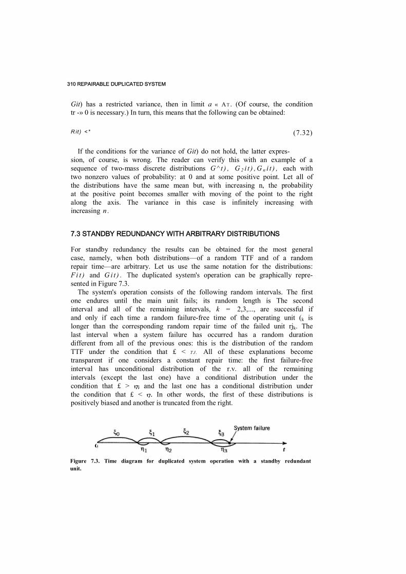
310 REPAIRABLE DUPLICATED SYSTEM
Git) has a restricted variance, then in limit a « AT . (Of course, the condition tr -» 0 is necessary.) In turn, this means that the following can be obtained:
R it ) <*
If the conditions for the variance of Git) do not hold, the latter expres- sion, of course, is wrong. The reader can verify this with an example of a sequence of two-mass discrete distributions G ^ t ) , G 2 i t ) , G n i t ) , each with two nonzero values of probability: at 0 and at some positive point. Let all of the distributions have the same mean but, with increasing n, the probability at the positive point becomes smaller with moving of the point to the right along the axis. The variance in this case is infinitely increasing with increasing n .
7.3 STANDBY REDUNDANCY WITH ARBITRARY DISTRIBUTIONS
For standby redundancy the results can be obtained for the most general case, namely, when both distributions—of a random TTF and of a random repair time—are arbitrary. Let us use the same notation for the distributions: Fi t ) and G i t ) . The duplicated system's operation can be graphically repre- sented in Figure 7.3.
The system's operation consists of the following random intervals. The first one endures until the main unit fails; its random length is The second interval and all of the remaining intervals, k = 2,3,..., are successful if and only if each time a random failure-free time of the operating unit (k is longer than the corresponding random repair time of the failed unit rjk. The last interval when a system failure has occurred has a random duration different from all of the previous ones: this is the distribution of the random TTF under the condition that £ < T J . All of these explanations become transparent if one considers a constant repair time: the first failure-free interval has unconditional distribution of the r.v. all of the remaining intervals (except the last one) have a conditional distribution under the condition that £ > 17; and the last one has a conditional distribution under the condition that £ < 17. In other words, the first of these distributions is positively biased and another is truncated from the right.
(7.32)
Figure 7.3. Time diagram for duplicated system operation with a standby redundantunit.
C
STANDBY REDUNDANCY WITH ARBITRARY DISTRIBUTIONS 311
Let £* denote a random value representing the system's time to failure starting from the moment + + • • • + g k . Here k is the num- ber of the last cycle when a system failure has occurred. For the distribution of the r.v. the following recurrent equation can be easily written:
1 - F* ( t ) = 1 - F( t ) - /"'[I - F* ( t - x)]G(*) d F( x ) (7.33)
The first term of the sum reflects the fact that during time ( no failure occurs. The expression under the integral means that the first failure occurs in the interval x + dx], but the repair of the failed unit has been completed up to this moment, and from this moment on the system is in the same state as in the previous moment at moment £0. Thus, this is the regeneration moment for the renewal process under consideration. The final goal is to find the distribution of the random value £0 + g* and to express the probability of the system's successful operation P ( t ) :
(7.34)
The numerical solution of (7.33) and (7.34) can be obtained by sequential iteration. But again we will use the LST which is useful for future asymptotic analysis. Introduce the following notation:
< p ( s ) = f d F* ( t ) J o
< p ( s ) = C e - d Q i t ) J n
Then the LST of (7.33) can be written as
< p ( s ) = <D( i) + « A(s ) [ l -< p( s ) ]
and, finally,
1 - 0 ( 5 )
o
o
(7.35)< p ( s ) =
STANDBY REDUNDANCY WITH ARBITRARY DISTRIBUTIONS 312
Combining (7.35) with (7.34), we get
< p ( s ) = &( s ) $ ( s ) - ® ( J)
From this LST, the system's MTTF can be found by setting 5 = 0. But in this case we prefer a more direct way:
= E { I 0) + E ( £ ^ \ - R + —
where v is the random number of cycles which has a geometric distribution with parameter a:
a - Al - G < r ) l < < F< 0 J o
which is small in practical cases. Let us investigate the asymptotic behavior of p i t ) . Suppose that F i t ) is fixed and the distribution of the repair time changes by some sequence in such a way that
«„= A l - 3 , ( 0 1 d F( t ) ^ 0 J n
Let us introduce the corresponding distributions and LSTs: Q„(t), <pn(s), il>„(s\ and, additionally, x„(s):
Xn(s) = <J»n(*) - </<„(*) - /V'[ 1 - G„(0j d F( t ) J o
Now we evaluate the difference
- x „( a n s ) = jf( 1 - - G„(t)} d F( t )
< a n s f t [ \ ~ G n ( t ) ] d Fi t ) o
C n f [ l - G n ( t ) } d F( t ) + f t d F( t ) Jo Jc„ £ a„s
If in this inequality we let
$ ( 0 - H f ) i -*(.)
(7.36)
C„ =

METHOD OF INTRODUCING FICTITIOUS STATES 313
then both terms in the last set of square brackets go to 0. This leads to the statement:
hm ----------- = 1 (i— a„
and the limit is uniformly exceeded on any finite area of domain of s . Now the normalized random variable anr is considered. The d.f. of this r.v, i s
Pr{A„T < r} = Q n
The LST of this d.f. is
For an -* 0, from (7.36) it follows that
< p n { a n s ) = 4>(anO 1 - <!>(«„$)
X „(<x„s) a
1 - <j>(a„Q + i + sT
and the limit is uniformly exceeded on any finite area of domain of s. Consequently,
lim Pr{dnr </} = !- e~"T (7.37) n —>oo
From (7.37) it follows that for a small value of a the approximation
nO = Pr{£syst > r}
is true.
7.4 METHOD OF INTRODUCING FICTITIOUS STATES
As we considered in Chapter 1, some combinations of exponential distribu- tions can produce distributions with both increasing and decreasing intensity

314 REPAIRABLE DUPLICATED SYSTEM
functions, or failure rates. This fact leads to the idea of an approximation of some arbitrary distributions. We will show that such an approximation can allow us to reduce semi-Markov processes to Markov processes.
A mixture of exponential distributions with different parameters leads to a distribution which has the decreasing intensity function
F ( t ) = Z = 1 " E P t e ~ » lS i S n 1Siin
A, # A y V( U) (7 -3 8 )
Pi > 0 v / , £ p f = l
A convolution of n identical exponential distributions e ( t ) = exp(-Ar) leads to an Erlang distribution of the «th order which can be expressed in the following recurrent way:
( A f ) " " ' NNR?(0 (7.39)
If there are exponential functions with different parameters e k { t ) = exp(-Ak t ) , then the generalized Erlang d.f. holds
^ ( 0 = e { * e 2 * ■ ■ ■ * e n { t ) = f ' e l * e 2 * ■ ■ ■ * e n _ t ( t - x ) d e „ ( x ) J o
(7.40)
Both the Erlang and the generalized Erlang distributions belong to the IFR class. Notice that the generalized Erlang d.f. can naturally approximate a wider subclass of distributions belonging to the IFR class.
It is reasonable to remember that the Erlang distribution represents an appropriate mathematical model for standby redundancy. Indeed, the pro- cess of a standby redundant group's operation can be described as a se- quence of a constant number of periods of a unit's successful operation.
Thus, (7.38) can be used as a possible approximation of the IFR distribu- tions, and (7.39) with (7.40) can be used for the DFR distributions. Of course, such an approximation leads to an increase in the number of states in the stochastic process under consideration. (Nothing can be obtained free, even

METHOD OF INTRODUCING FICTITIOUS STATES 315
in mathematics!) But we should mention that the process itself becomes much simpler: it becomes purely Markov. At the same time, such an approxi- mation is good only for systems of a very restricted size.
For simplicity of further illustrations, we will consider only cases where the initial distributions are approximated with the help of combinations of two exponential distributions. We should mention that the problem of determin- ing an appropriate approximation of a distribution with monotone failure rates by the means of (7.38) to (7.40) is a special problem lying outside of the scope of this book.
Now we illustrate the main idea by means of simple examples.
IFR Repair Time and Exponential Time to Failure For some applied problems it is natural to use the exponential distribution for a random TTF. At the same time, to assume an exponential distribution for the repair time might seem strange: why should the residual time of repair not depend on the time already spent? If a repair involves a routine procedure, a more realistic assumption involves the IFR distribution of this r.v. To make this statement clearer, we consider a repair process as a sequence of several steps: if one step is over, the residual time of repair is smaller because now it consists of a smaller number of remaining steps.
In this case two failure states might be introduced for a unit: state 1 and state 1*, both with an exponentiatly distributed time remaining in each of them. These sequential states represent the series sequence of two stages of repair (see Figure 7.4a). The total random time of staying in a failed state subset is the sum of two exponentially distributed random variables and, consequently, will have an IFR distribution. Incidentally, in this case (7.40) has the following expression:
— - ( 7 ,4 1 )
A, — A2
Figure 7.4. Transition graphs for a multistate model of renewable units: («) with an IFR distributed repair time and an exponentially distributed failure-free time;

316 REPAIRABLE DUPLICATED SYSTEM
(ft) with an IFR distributed failure-free time and an exponentially distributed repair time.
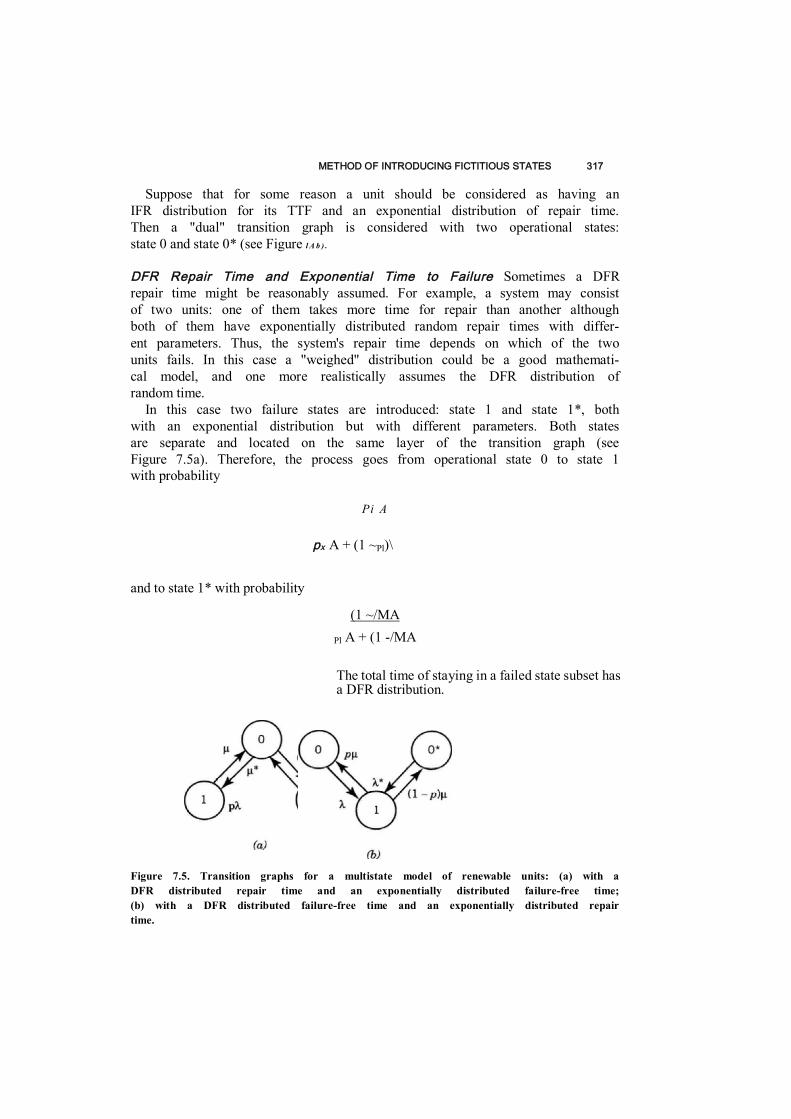
METHOD OF INTRODUCING FICTITIOUS STATES 317
Suppose that for some reason a unit should be considered as having an IFR distribution for its TTF and an exponential distribution of repair time. Then a "dual" transition graph is considered with two operational states: state 0 and state 0* (see Figure l A b ) .
DFR Repair Time and Exponential Time to Failure Sometimes a DFR repair time might be reasonably assumed. For example, a system may consist of two units: one of them takes more time for repair than another although both of them have exponentially distributed random repair times with differ- ent parameters. Thus, the system's repair time depends on which of the two units fails. In this case a "weighed" distribution could be a good mathemati- cal model, and one more realistically assumes the DFR distribution of random time.
In this case two failure states are introduced: state 1 and state 1*, both with an exponential distribution but with different parameters. Both states are separate and located on the same layer of the transition graph (see Figure 7.5a). Therefore, the process goes from operational state 0 to state 1 with probability
Pi A
px A + (1 ~Pl)\
and to state 1* with probability
(1 ~/MA
Pl A + (1 -/MA
The total time of staying in a failed state subset has a DFR distribution.
Figure 7.5. Transition graphs for a multistate model of renewable units: (a) with a DFR distributed repair time and an exponentially distributed failure-free time; (b) with a DFR distributed failure-free time and an exponentially distributed repair time.
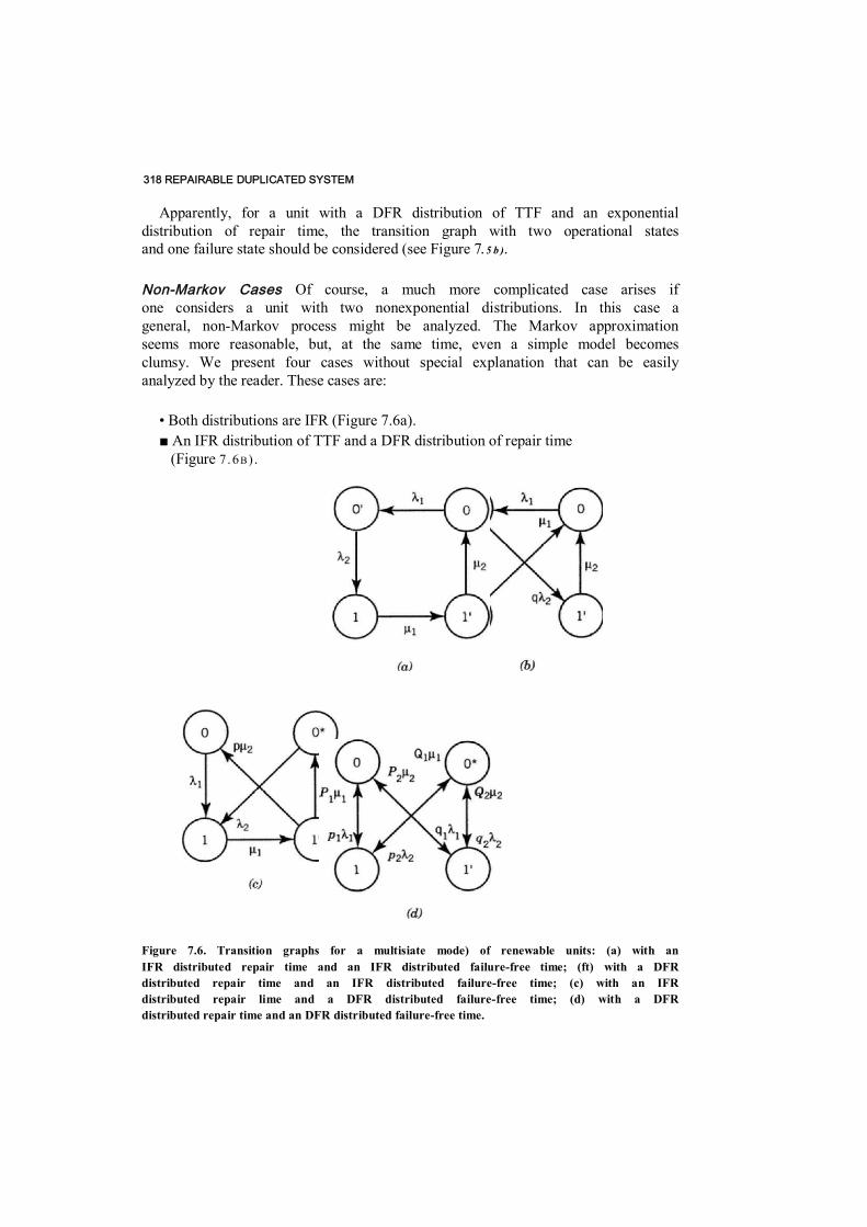
318 REPAIRABLE DUPLICATED SYSTEM
Apparently, for a unit with a DFR distribution of TTF and an exponential distribution of repair time, the transition graph with two operational states and one failure state should be considered (see Figure 7. 5 b ) .
Non-Markov Cases Of course, a much more complicated case arises if one considers a unit with two nonexponential distributions. In this case a general, non-Markov process might be analyzed. The Markov approximation seems more reasonable, but, at the same time, even a simple model becomes clumsy. We present four cases without special explanation that can be easily analyzed by the reader. These cases are:
• Both distributions are IFR (Figure 7.6a). ■ An IFR distribution of TTF and a DFR distribution of repair time
(Figure 7.6B) .
Figure 7.6. Transition graphs for a multisiate mode) of renewable units: (a) with an IFR distributed repair time and an IFR distributed failure-free time; (ft) with a DFR distributed repair time and an IFR distributed failure-free time; (c) with an IFR distributed repair lime and a DFR distributed failure-free time; (d) with a DFR distributed repair time and an DFR distributed failure-free time.
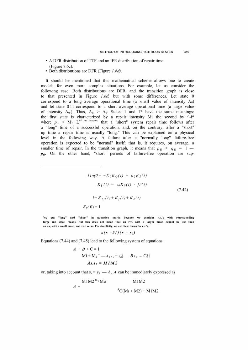
METHOD OF INTRODUCING FICTITIOUS STATES 319
• A DFR distribution of TTF and an IFR distribution of repair time (Figure 7.6c).
• Both distributions are DFR (Figure 1.6d).
It should be mentioned that this mathematical scheme allows one to create models for even more complex situations. For example, let us consider the following case. Both distributions are DFR, and the transition graph is close to that presented in Figure 1.6d, but with some differences. Let state 0 correspond to a long average operational time (a small value of intensity A0) and let state 0 11 correspond to a short average operational time (a large value of intensity A0.). Thus, Aa, > A0. States 1 and 1* have the same meanings: the first state is characterized by a repair intensity Mi the second by ^-i* where p.r > Mv L61 us assumc that a "short" system repair time follows after a "long" time of a successful operation, and, on the contrary, after a "short" up time a repair time is usually "long." This can be explained on a physical level in the following way. A failure after a "normally long" failure-free operation is expected to be "normal" itself; that is, it requires, on average, a smaller time of repair. In the transition graph, it means that p Q > q Q = 1 — pQ. On the other hand, "short" periods of failure-free operation are sup-
11o(0 = ~ X 0 K Q ( t ) + p 2 K 2 ( t )
K [ ( t ) = \ 0 K 0 ( t ) - f i ^ t ) (7.42)
l = K { } ( t ) + K ] ( t ) + K 2 ( t )
K0( 0) = 1
'we put "long" and "short" in quotation marks because we consider r.v.'s with corresponding large and small means, but this does not mean that an r.v. with a larger mean cannot be less than an r.v, with a small mean, and vice versa. For simplicity, we use these terms for r.v.'s.
s ( s - 5 i ) ( s - s2 )
Equations (7.44) and (7.45) lead to the following system of equations:
A + B + C = 1 Mi + M2 = —A ( s , + s2) — BS 2 — C$j
As i s2 = M 1 M 2
or, taking into account that s, = s2 — b, A can be immediately expressed as
M1M2 m \ M a M1M2 A =
AO(MI + M2) + M1M2

320 REPAIRABLE DUPLICATED SYSTEM
posed to be connected with some kind of "serious" failure, which leads to a "long" repair time. In the transition graph, this means that pQ. > q(). = 1 - /v-1
Of course, the inverse situation might be considered. Explanations also seem very reasonable: a "long" repair might follow a "long" period of successful operation. Indeed, we expect more failures of redundant units may appear during the longer period of time. As usual, a narrative of the system, which is taken to be a basis for the mathematical model, depends on the concrete actual nature of the system under investigation. For systems consist- ing of several units such an approximation may lead to difficulties in the construction of the corresponding transition graph.
Let us consider the simple case represented in Figure 7.4a in more detail. Incidentally, this case shows the special behavior of the availability coeffi- cient. The system of differential equations is constructed in the usual way:
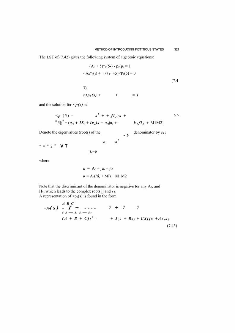
METHOD OF INTRODUCING FICTITIOUS STATES 321
The LST of (7.42) gives the following system of algebraic equations:
(A0 + 5)^0(5-) - p2(p2 = 1
- A0*0(i) + ( f l y +5)<Pi(5) = 0
(7.4
3)
s<p 0 (s) + + = 1
and the solution for <p(s) is
< p ( 5 ) = s 2 + + f i 2 ) s + ^ ^ 0 5[j2 + (A0 + IX , + ix2 )s + A0ju, + k 0 f i 2 + M1M2]
Denote the eigenvalues (roots) of the denominator by sk :
a a 2 ^ = " 2 ± V T
53 = 0
where
a = A0 + ju, + jt2
b = A0(/ti, + Mi) + M1M2
Note that the discriminant of the denominator is negative for any A0, and H2, which leads to the complex roots jj and s2 . A representation of <p0(s) is found in the form
A B C <Po( s ) - T + - - - - 7 + 7 7
s s — s, s — s2 ( A + B + C ) s 2 - + 5 2 ) + Bs2 + C S ] ] s + A s t s 2
- b
(7.45)
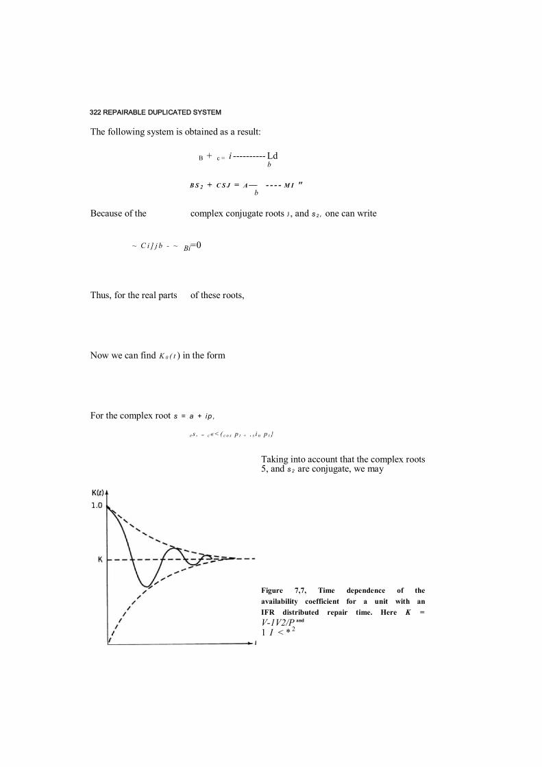
322 REPAIRABLE DUPLICATED SYSTEM
The following system is obtained as a result:
B + c = i ---------- Ld b
B S 2 + C S J = A — - - - - M I " b
Because of the complex conjugate roots J , and s 2 , one can write
~ C i ] j b - ~ =0
Thus, for the real parts of these roots,
Now we can find K 0 ( t ) in the form
For the complex root s = a + ip ,
e s , = c « < ( c o s p t + , s i n p t }
Taking into account that the complex roots 5, and s 2 are conjugate, we may
Figure 7,7, Time dependence of the availability coefficient for a unit with an IFR distributed repair time. Here K = V-1V2/P and 1 I < * 2
Bi

METHOD OF INTRODUCING FICTITIOUS STATES 323
t

324
REPAIRABLE DUPLICA
TED SYSTEM
write
The final result is
*o(') «
In this particular case the nonstationary availability coefficient is periodically oscillating with a decreasing amplitude (see Figure 7.7).
7.5 DUPLICATION WITH SWITCH AND MONITORING
Because of their relative simplicity, the mathematical models of a duplicated system with renewal allow one to consider some sophisticated cases close to real situations. Indeed, most "classical" mathematical models of redundant systems with repair are based on the assumption that the redundant group of units has an ideal switch which performs its functions reliably, without errors and delays. Moreover, the units are supposed to be totally and continuously monitored; that is, the occurrence of an operating or redundant unit failure becomes known immediately. It is clear that such assumptions are far from real. Sometimes, of course, these factors may be neglected. (But only some- times!)
When a duplicated system is described by a Markov model, it is possible to provide an analysis of reliability by accounting for some additional factors. Obviously, it does not lead to especially clear and understandable models. At any rate, the solution can be derived.
Below we consider several examples which illustrate how one may con- struct appropriate mathematical models. We will not present the final results because they are inevitably bulky. A computer must be used for the numeri- cal calculations. But, as is well known, no computer can substitute for the human mind, at least during the first stage of any research: one needs to be able to construct an appropriate mathematical model and only after this may one resort to computer calculation.
7.5.1 Periodic Partial Control of the Main Unit
e~*i' + e-*2< = 2 cos
M1M2 b
+

DUPLICATION WITH SWITCH AND MONITORING 325
We start with a simple example. A duplicated system consists of two indepen- dent identical units. One of them is in an operating position (the main unit) and the other is in a redundant position. The unit's failure rate depends on the current occupied position: operating or waiting. Let us assume that only

326 REPAIRABLE DUPLICATED SYSTEM
part of the main unit can be monitored continuously. The state of the remaining nonmonitored part of the main unit can be checked only periodi- cally. In other words, if a failure has occurred in the nonmonitored part of the main unit, no switching to replace this failed unit is performed. A periodic test discovers that the main unit has failed and only then the switching might be performed. Thus, before this test, the duplicated system remains in a state of "hidden failure." The switching is assumed to be instantaneous. The redundant unit is continuously monitored, so a repair of the failed redundant unit begins instantly after a failure has occurred. Of course, the same thing happens if a failure occurs in the monitored part of the main unit.
During a repair of the main unit, all of its failures—both in the monitored and nonmonitored parts—are deleted. In other words, the repaired unit becomes as good as new. As soon as the failure of the main unit is detected (by any means—continuous or periodical monitoring), the redundant unit is switched into the main position. After repair, the unit becomes the redun- dant one. If one finds both units have failed, the total system repair is performed. After repair, the system, as a whole, becomes as good as new.
For the use of a Markov model, let us assume that monitoring is provided at randomly chosen moments of time. Moreover, assume that the distribution of the length of the periods between the tests is exponential. We mention that such an assumption is sometimes close to reality: in a computer, tests can be applied between runs of the main programs, and not by a previously set strict schedule.
The transition graph for this case is presented in Figure 7.8. The following notation is used in this example:
• M is the operational state of the main unit. • M * is the "hidden failure" of the main unit. • M is the failure state of the main unit. • R is the operational state of the redundant unit. • R is the failure state of the redundant unit. • A, is the failure rate of the nonmonitored part of the main unit. • A, is the failure rate of the monitored part of the main unit. • A is the failure rate of the redundant unit. • /x is the intensity of repair of a single unit. • M* is the intensity of repair of the duplicated system as a whole. • v is the intensity of periodical tests.
The transition graph presented in Figure 7.8a is almost self-explanatory. Notice that for this case there arc two states of system failure: [M* /i] and [ M R] , These failure states are denoted by bold frames in the figure.

DUPLICATION WITH SWITCH AND MONITORING 327
We will not describe the routine procedure of finding the reliability indexes. Our main goal is to build a mathematical model from the verbal description and to clarify all of the needed assumptions.
7.5.2 Periodic Partial Monitoring of Both Units The duplicated system consists of two identical independent units. One of them is in an operating position (the main unit) and the other is in a
Figure 7.8. Transition graphs for a duplicated system with a partially monitored main unit: (a) graph including instantaneous "jumps" (intensity equal to (b) equivalent
graph excluding the state in which the system spends no time.

328 REPAIRABLE DUPLICATED SYSTEM
redundant position. The unit's failure rate depends on the occupied position: operating or waiting. Let us assume that only a part of each unit can be monitored continuously. (The monitored parts are identical in both units.) The state of the remaining nonmonitored parts of each of these units can be checked only periodically. Tests of the main and redundant units have different periods (intensity). The switching system is analogous to that described in the previous example. If one knows that both units have failed, the repair is performed until complete renewal of the system. Let us consider two possible means of repair: (a) there are independent repair facilities for each unit, and (b) there is only one repair facility. After repair, the unit becomes as good as new. The transition graph for this case is presented in Figure 7.9. The following notation is used in this example:
* M is the operational state of the main unit. * M * is the "hidden failure" of the main unit. - M is the failure state of the main unit. * R is the operational state of the redundant unit, * R * is the "hidden failure" of the redundant unit. - R is the failure state of the redundant unit, * A, is the failure rate of the nonmonitored part of the main unit. * Aj is the failure rate of the monitored part of the main unit. * A is the failure rate of the nonmonitored part of the redundant unit. * A is the failure rate of the monitored part of the redundant unit. * fi is the intensity of repair of a single unit. - n* is the intensity of repair of the duplicated system when there are two
failed units, * y, is the intensity of periodic tests of the main unit, * v is the intensity of periodic tests of the redundant unit.
The transition graph presented in Figure 7.9 is almost self-explanatory. We only discuss the following two transitions:
1. [M R*] to [M R ] : This transition occurs if (a) an extra failure appears in the continuously monitoring part of the redundant unit or (b) the periodic test has found a "hidden failure."
2. [Af /?*] to [ M * J?]: This transition occurs if a failure appears in the continuously monitoring part of the main unit. Then the main unit is directed to repair and is substituted by the redundant one with a "hidden failure."
These failure states are again denoted by bold frames in the figure.
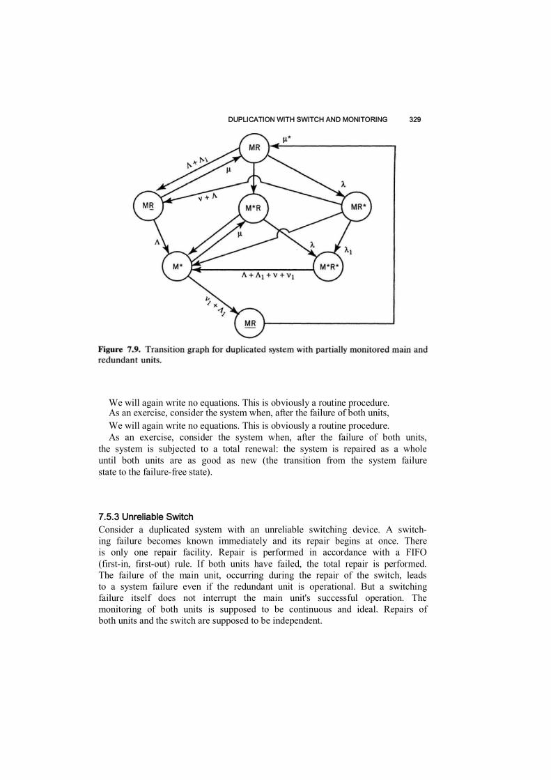
DUPLICATION WITH SWITCH AND MONITORING 329
We will again write no equations. This is obviously a routine procedure. As an exercise, consider the system when, after the failure of both units, We will again write no equations. This is obviously a routine procedure. As an exercise, consider the system when, after the failure of both units,
the system is subjected to a total renewal: the system is repaired as a whole until both units are as good as new (the transition from the system failure state to the failure-free state).
7.5.3 Unreliable Switch Consider a duplicated system with an unreliable switching device. A switch- ing failure becomes known immediately and its repair begins at once. There is only one repair facility. Repair is performed in accordance with a FIFO (first-in, first-out) rule. If both units have failed, the total repair is performed. The failure of the main unit, occurring during the repair of the switch, leads to a system failure even if the redundant unit is operational. But a switching failure itself does not interrupt the main unit's successful operation. The monitoring of both units is supposed to be continuous and ideal. Repairs of both units and the switch are supposed to be independent.

330 REPAIRABLE DUPLICATED SYSTEM
The transition graph for this case is presented in Figure 7.10. The follow- ing notation is used in this example:

DUPLICATION WITH SWITCH AND MONITORING 331
As in the previous examples, the transition graph presented in Figure 7.10 is almost self-explanatory. We only discuss the following transitions:
1. [ M R 5] to [ M R 5]: This transition occurs if the switch has been repaired: at the moment of the termination of repair, the redundant unit is instantly directed to the position of the failed main unit, and the latter begins to be considered as a redundant unit directed to repair.
2. [ M R 5] to [ M R 5] and [ M R 5] to [ M R 5]: These two transitions depend on which unit is repaired first: if the switching device is in repair, it is impossible to put the repaired redundant unit into the position of the main unit.
These failure states are again denoted by bold frames in the figure.
7.5.4 Unreliable Switch and Monitoring of Main Unit A duplicated system consists of two identical independent units: main and redundant. The unit failure rate depends on the occupied position. Let us assume that only a part of the main unit can be monitored continuously. The state of the remaining nonmonitored part of the unit can be checked only periodically. The switching device works as described above. Repairs of both the units and the switch are independent. After repair, a unit (or a switch) becomes as good as new.
The transition graph for this case is presented in Figure 7.10. The follow- ing notation is used in this example:
CONCLUSION 332
Note that the switching device may be one of the two following main types: (a) as we considered before, a switching failure does not interrupt the system's operation, or (b) a switching failure interrupts the system operation. In the latter case, the switch is a necessary part of the system. This may occur, for example, if the switch plays the role of an interface between the duplicated system's output and the input of another system or subsystem.
Of course, there are many other concrete examples of this type. We can only repeat that our main goal is to explain the methodology of modeling and not to give a list of the results or to make the reader exhausted with boring solutions of bulky equations.
The mathematical techniques used in this section are simple enough. But the results obtained are not always very clear or "transparent" for further analysis: What will happen if one changes some parameters? What will happen if the switching or monitoring methods are changed? Of course, in practical situations an engineer would like to have correct and simple formulas to perform a quick and understandable analysis of the designed system. Fortunately, for highly reliable systems (we emphasize again that this is the most important practical case!), it is possible to develop such simple and sufficiently accurate methods. The reader can find such methods in Chapter 13 dedicated to heuristic methods in reliability.
CONCLUSION
It seems that the first paper on the analysis of a duplicated system with repair (renewal) was published by Epstein and Hosford (1960). They solved the problem foT a purely Markov model when the distributions—both TTF and repair time—were exponential. They solved the problem with the help of birth and death processes. Their model is also described in Gnedenko and Kovalenko (1987). Here the solution of the same problem for the duplicated system was found for both active and underloaded redundancy.
A systematic investigation of renewal systems, in particular, the duplicated system, may be found in Ushakov (1985, 1994). Belyaev (1962) developed an elegant method of so-called "striping Markov processes" which has allowed one to solve the problem with no assumption of exponentiality on the repair time. Independently, Gaver (1963) obtained practically the same results with the help of traditional methods.
Gnedenko (1964a, 1964b) obtained solutions for the general case when both distributions are arbitrary. Theorems concerning the asymptotic behav- ior of renewal duplicated systems have been obtained by D. Gnedenko and Solovyev (1974, 1975). and, practically simultaneously, by Gnedenko, Belyaev, and Solovyev (1969). The method of fictitious states (stages) for "Markoviza- tion" of non-Markov models as applied to queuing systems takes its origin from Erlang's work. A comprehensive exposition of existent mathematical results related to the problem can be found in Ushakov (1985, 1994), where
EXERCISES 333
results conccrmng the various models of duplicated renewal systems are presented. A detailed review of asymptotic methods is given by Gertsbakh (1984).
REFERENCES
Belyaev, Yu. K. (1962). Striping Markov processes and their applications to reliability problems (in Russian). Proc, Fourth All-Union Meeting on Probab. Theory Math. Statist., Vilnius (Lithuania), pp. 309-323. Epstein, B.. and T. Hosford (1960). Reliability of some two unit redundant systems. Proc. Sixth Nat. Symp. on RQC, pp. 466-476. Gavcr, D. P, (1963). Time to failure and availability of parallel systems with repair.
IEEE Trans. RQC, vol. R-12, pp. 30-38. Gertsbakh, I. B. (1984). Asymptotic methods in reliability theory: a review. Ada. in Appl. Probab. vol. 16. Gnedcnko, B. V. (1964a). On duplication with renewal, Engrg. Cybernet., no. 5, pp. 111-118. Gnedcnko, B. V. (1964b). On spare duplication. Engrg. Cybernet., no. 4, pp. 3-12. Gnedcnko, B. V., and 1. N. Kovalenko (1987). Introduction to Queuing Theory, 2nd ed. (in Russian). Moscow: Nauka. Gnedcnko, B. V„ Yu. K. Belyaev, and A, D. Solovyev (1969). Mathematical Methods
of Reliability Theory. New York: Academic. Gnedenko, D. B., and A. D. Solovyev (1974). A general model for standby with renewal. Engrg. Cybernet., vol. 12, no. 6. Gnedenko, D. B., and A, D. Solovyev (1975). Estimation of the reliability of complex renewable systems. Engrg. Cybernet., vol, 13, no. 3. Solovyev, A. D. (1970). Standby with rapid repair. Engrg. Cybernet., vol. 4, no. I. Solovyev, A. D. (1971). Asymptotic behavior of the time of first occurrence of a rare event. Engrg. Cybernet., vol. 9, no. 3. Solovyev, A. D. (1972). Asymptotic distribution of the moment of first crossing of a high level by birth and death process. Proc. Sixth Berkeley Symp. Math. Statist. Probab., Issue 3. Ushakov, I. A„ ed. (1985). Reliability of Technical Systems: Handbook (in Russian). Moscow: Radio i Sviaz, Ushakov, I. A., ed, (1994). Handbook of Reliability Engineering. New York: Wiley,
EXERCISES
7.1 There are two transition graphs (see Figures E7.1« and b). State 2 is a failed state in both cases. (a) Give a verbal description of the two systems to which these graphs
correspond. (b) Which system has a larger MTTF?

334 REPAIRABLE DUPLICATED SYSTEM
(c) Which system has a larger MTBF? (d) What is the difference between the MTTF and MTBF of the first
system? (e) Which system has a larger mean repair time?
/ -X 0.5\i
0h
2 X
Q
X 1 f
Figure E7.1.
7.2 Depict a transition graph for a unit with an exponentially distributed time to failure and a repair time having an Erlang distribution of the third order.
7.3 Depict a transition graph for a renewable unit with an exponentially distributed time to failure. P ( t ) = e ~ X l , and with a repair time dis- tributed as
G ( / ) = Pi <?"Ml' + p 2 + p 3
7.4 Given an interpretation of the transition graph depicted in Figure E7.4.
0 2X
2 H
3
© 2 \
© 2ft
0
Mv)

EXERCISES 335
Failure Figure E7.4.
0 Failure
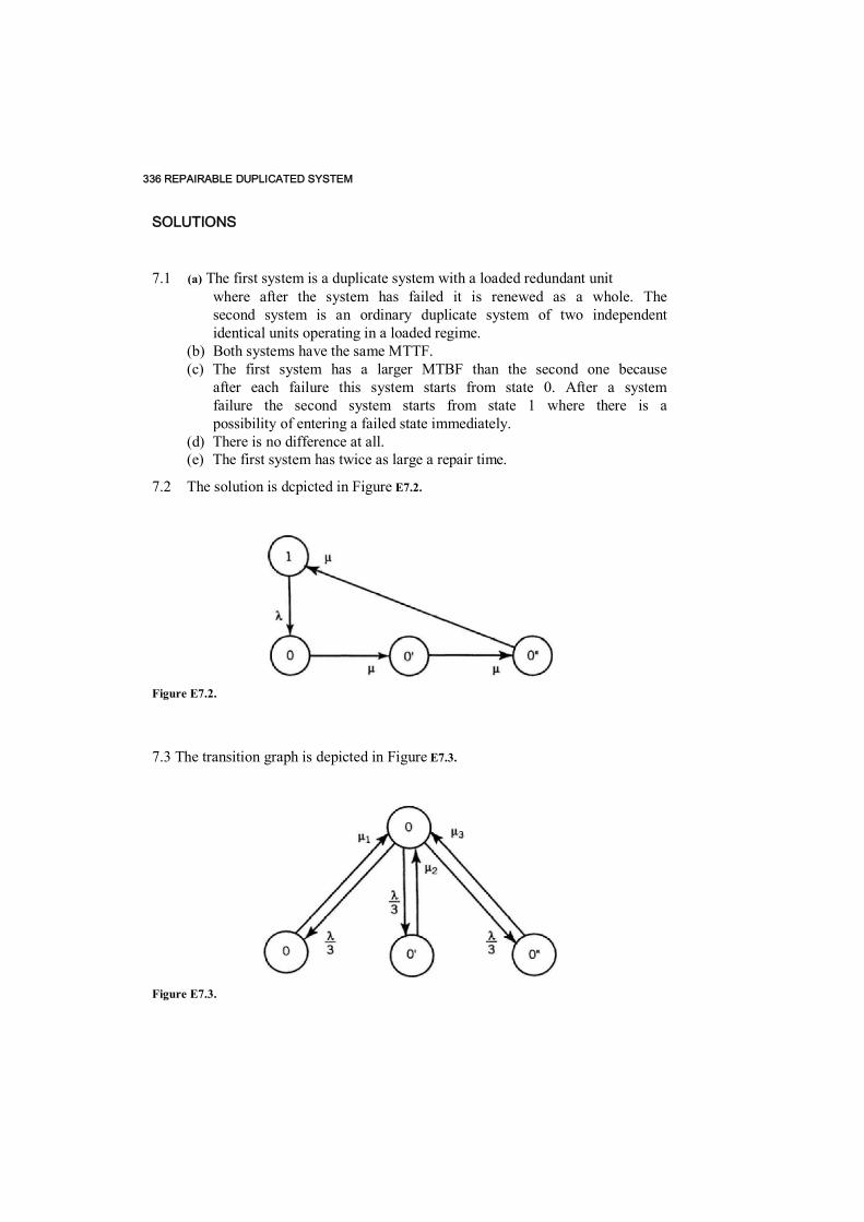
336 REPAIRABLE DUPLICATED SYSTEM
SOLUTIONS
7.1 (a) The first system is a duplicate system with a loaded redundant unit where after the system has failed it is renewed as a whole. The second system is an ordinary duplicate system of two independent identical units operating in a loaded regime.
(b) Both systems have the same MTTF. (c) The first system has a larger MTBF than the second one because
after each failure this system starts from state 0. After a system failure the second system starts from state 1 where there is a possibility of entering a failed state immediately.
(d) There is no difference at all. (e) The first system has twice as large a repair time.
7.2 The solution is dcpicted in Figure E7.2.
Figure E7.2.
7.3 The transition graph is depicted in Figure E7.3.
Figure E7.3.
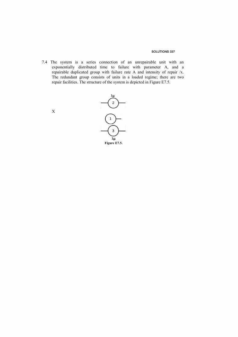
SOLUTIONS 337
7.4 The system is a series connection of an unrepairable unit with an exponentially distributed time to failure with parameter A, and a repairable duplicated group with failure rate A and intensity of repair /x. The redundant group consists of units in a loaded regime; there are two repair facilities. The structure of the system is depicted in Figure E7.5.
X
Figure E7.5.
CHAPTER 8
ANALYSIS OF PERFORMANCE EFFECTIVENESS
8.1 CLASSIFICATION OF SYSTEMS
8.1.1 General Explanation of Effectiveness Concepts Modern large-scale systems are distinguished by their structural complexity and their requirements for sophisticated algorithms to facilitate the function- ing and interacting of their subsystems. On the one hand, this allows them to fulfill many different operations and functions, while, on the other hand, it leads to stable operations with a sufficient level of effectiveness even with some failed units and subsystems and/or under extreme influences of the external environment.
The adaptation of a complex system to external influences and to internal perturbations is possible only because of the redundancy of the system's structure and its ability to readjust its functions under various circumstances. In other words, the feature of modern technical systems is not only an extreme increase in the number of interacting units but also the appearance of entirely new qualitative properties. One of these properties is the stability of operation mentioned above.
It is also very important that modern large systems, such as information systems (computer and communications networks, control systems, etc.), energy systems (electric power networks, oil and gas pipelines, etc.), and transportation systems (railroads, highways, airlines, etc.) are multifunctional. Such systems, as a result of external and internal influences, can perform some functions perfectly and, at the same time, completely interrupt the performance of other functions. This means that, according to one criterion, a system as a whole could be considered successful and, by another criterion, 298

CLASSIFICATION OF SYSTEMS 339 Probabilistic Reliability Engineering. Boris Gnedenko and Igor Ushakov
340 ANALYSIS OF PERFORMANCE EFFECTIVENESS
it could be considered failed. A researcher encounters the usual difficulties associated with multicriteria analysis.
But even for a complex system predestinated for one type of operation, there is generally no strict definition of failure. Often in such systems even a significant set of failed units could lead only to a decrease in performance and not to a complete system failure. This happens because of a partial "overlapping" of different subsystem (unit) functions, the presence of differ- ent feedbacks, the means of error correction, and so forth.
We consider several simple examples. In a regional power system, a failure of some subsystem (e.g., the failure of the fuel transportation system of an electric power plant) can be compensated for by using fuel from storage. In another case a deficiency of energy can be compensated for by a partial increase in the power of neighboring plants. Sometimes clients might use another type of energy supply. Under conditions of a severe energy deficit, clients with lower levels of priority might be temporarily "turned off" from an energy system in order to decrease the total damage.
Sometimes a completely operational system might be unable to perform some of its functions because of a harmful coincidence of external circum- stances. For example, consider a communications network. All equipment in the system could be in a perfect operating state, but weather may spoil the opportunity to use certain radio channels. The same effect may be observed if there is some neighboring influence of other radio transmission systems. Even network users may create excessively heavy communication traffic which can lead to system performance failures.
Of course, from a client's viewpoint, he or she is quite indifferent to the reason for a breakdown in communication: either it happens because of a system failure or because of an overloading of the communications network.
For all such systems it is natural to speak about performance effectiveness. In each concrete case the index (or indexes) of performance effectiveness should be chosen with respect to the type of system under consideration, its destination, conditions of operation, and so forth. The physical characteris- tics of the performance effectiveness index (PEI) are usually completely defined by the nature of the system's outcome and can be evaluated by the same measures. In most practical cases we can measure a system's effective- ness in relative units. We might take into account the nominal (specified) value of a system's outcome as the normalizing factor. In other words, the PEI is a measure of the quality and/or volume of the system's performed functions or operations; that is, it is a measure of the system's expediency.
Of course, a system's efficiency is not an absolute measure. It depends on the type of functions and tasks being performed and the operating environ- ment. A system which is very efficient under some circumstances and for some operations might be quite useless and ineffective under another set of circumstances and/or operations.
In general, a PEI is dimensional. The dimension of the PEI depends on the system's outcomes, as we mentioned above. When it is possible in the

INSTANT SYSTEMS 341 following discussion, we shall consider the PEI as a ratio of the expected system outcome to its maximal outcome. In this case the PEI is nondimen- sional. Of course, we always assume a larger outcome is a better outcome. The use of a nondimensional PEI is very convenient in many practical evaluations.
Sometimes we encounter "pessimistic" measures which characterize a system's performance. For example, consider the acceptable error of a technological process or the permissible volume of pollution of a plant. Such indexes measure "ineffectiveness" rather than effectiveness. Usually, in such cases one can reformulate the desired outcome in "positive" terms.
If a system's outcome has an upper bound, the PEI can be expressed in a normalized form; that is, it may be considered as having a positive value lying between 0 and 1. Then we have PEI = 0 if the system has completely failed and PEI = I when it is completely operational. For intermediate states, 0 < PEI < 1.
When considering a system's effectiveness, one should remember the property of monotonicity introduced earlier. In this context, an increase in the reliability of any unit leads to a simultaneous increase in the system's effectiveness. Also, a failure of any unit can only decrease (not increase) a system's effectiveness.
It is convenient for system design to determine a PEI in relative units, because in this case one docs not need to measure an absolute value of a system's outcomc for different states. The absolute values of a PEI are very convenient if we must compare several different competitive variants of a system. They allow us to compare variants of a system with different reliabil- ity and different efficiencies of performance. It is clear that reliability alone does not completely solve the problem of engineering design.
8.1.2 Classes of Systems Consider a system consisting of n units. As before, we suppose that any system unit has two states: an operating state and a failed state. Let xt be the indicator of the ith unit's state: xt = 1 when the unit is up and Xj = 0 when the unit is down. The system then has 2" different states as determined by the states of its units. Denote a system state by X = (xlt x 2 , . . . , x n ) .
If we consider the process of a system's evolution in state space, then for each unit we should consider the process *,-(*), and for the system as a whole, the process X ( t ) . The transformation of system states X(r) character- izes the system's behavior. On the basis of knowledge about this process, we can analyze a system's effectiveness.
Taking into account the length of a system's performance, it is reasonable, for effectiveness analysis, to distinguish two main classes of systems: instant and enduring.
Some systems are characterized by their instant outcomc at a moment of time. The current effectiveness of an instant system is completely determined
342 ANALYSIS OF PERFORMANCE EFFECTIVENESS
by its state at the moment of performance. It is clear that no instant system exists in reality because any task has some duration. Strictly speaking, we consider a system whose duration of performance is negligibly short in comparison with time intervals between changing system states X(f). This means that
P{ X ( t ) = X ( t + t 0 ) } = 1 - e ( 8 . 1 )
where f0 is the system's task duration and e is a practically negligible value. (The size of e depends on the required accuracy of analysis.)
From (8.1) it follows that the current effectiveness of a system is completely determined by the current system state X = X(r). For this state the effec- tiveness coefficient equals Wx, and the system's PEI can be determined as the expected value of Ifx.
Examples of practical instant systems are missiles, production lines (during production of a single item), and a communications network during an individual call.
For an enduring system condition (8.1) is not valid. The effectiveness of an enduring system depends on a trajectory of the system's transition from one state to another. In this case the fact that some particular units have failed is very important, but the moments and the order of their failures are also equally important. In other words, for these systems the effectiveness is determined by a trajectory of states changing during the system's perfor- mance of a task.
Examples of enduring systems are different technological and chemical processes, information and computer systems, aircraft, and so on.
8.2 INSTANT SYSTEMS
Let h X / ( t ) denote the probability that an instant system at moment t is in state Xfc(/). We assume that the current effectiveness of the system being in any state can be evaluated. Let us denote this value for state X as lfx. It is natural to determine W as the expected value of W x , that is,
= E h X k ( t ) W X k
(8.2)
1 S t s N
where N = 2" is the total number of different system states. It is clear that an absolutely accurate calculation of a system's effectiveness
when n 1 is a difficult, if not unsolvable, computational problem. First of all, it is connected with the necessity of determining a large number of coefficients Wk. Fortunately, it is sometimes not too difficult to split all of the system's states into a relatively small number of classes with close values Wk.

INSTANT SYSTEMS 343 If so, we need only to group appropriate states and calculate the correspond- ing probabilities. W^, can then be calculated as
KysM = E W, E M < ) (8-3>
where M is the number of different levels of the values of W x and G j is the set of system states for which IVX belongs to the j'th level. Later we shall consider special methods for the evaluation of the effec- tiveness of higher-dimensional systems. Let us evaluate a system's effectiveness for a general case. For notational simplicity, we omit the time t in the expressions below. Let h 0 denote the probability that all units of the system are successfully operating at moment
K - n P i (8-4) 1 sisn
Let h , denote the probability that only the ;'th unit of the system is in a down state at moment / (repairable systems can be considered as well as unre- pairable). Then
hi - qt II Pi = ~ho = SiK (8.5) 1 <,)<,n Pi j+i
where, for brevity, we introduce gt = ql/p< and h t j denotes the probability that only the ith and jth units of the system are in down states at moment t :
h i j ^ l . l i El Pk = ^Lh0 = 8 , S j h 0 (8.6) 1 <.!<.n P,Pj k * U J )
and so on. We can write the general form of this probability as
- n P i n * - n * (8-7> / ^ C j i e C , i e C ,
where G x is the set of subscripts of the units which are considered opera- tional in state X and Gx is the complementary set. Sometimes it is reason- able to write (8.7) for any X as
*x= n p M1
~x
» (8-8) 1 sisn
It is clear that (8.7) and (8.8) arc equivalent. Using (8.4) to (8.8), we can
344 ANALYSIS OF PERFORMANCE EFFECTIVENESS
rewrite (8.3)
1+ E wigi + E wlj8igj +
l i i ^ n lsic/sn
where W0 is the system effectiveness for state X0 and Wt, W t j , . .. are normalized effectiveness coefficients for states X,, \tj ................... In other words, W, = W(/W0, Wu = WSJ/1V0,... .
For a system consisting of highly reliable units, that is,
1 max q* « — I s i s n r t
expression (8.9) can be approximated as
Wsys. - - E E W i q \ ~ W Q ( \ - E <?>,) (8.11) V 1 zi<,n l s i s n ' V li/'i/i '
Here w, = 1 - W i has the meaning of a "unit's significance." REMARK. It is necessary to note that, strictly speaking, it is wrong to speak of a "unit's significance." The significance of a unit depends on the specific system state. For example, in a simple redundant system of two units, the significance of any unit equals 0 if both units are successfully operating, but if a single unit is operating at the time, then its significance equals 1. Other examples are considered below.
Consider some particular cases of (8.11). If p,(/) = exp(-A;/) is close to 1 and, consequently, <7,(r) = A,f, then (8.11) can be approximated by
" W o f l " E 9,(<k) exp
We can see that "the significance of unit" is reflected, in this case, in the factual failure rate. (See the previous remark.)
If pt is a stationary availability coefficient, that is, p, = 7]/(7] + r,) where Ti is the MTBF of the z'th unit and r, is its idle time and » r,, then it is possible to write the approximation
^syst ~ W0
(8.9)^sysl _
(8.10)
■ t E A , . ( l - ^ )
1 <.i<.n WK (8.12)sysi
i- E
(8.13)T1S i S n ' i

INSTANT SYSTEMS 345
Again, we can consider "the significance of a unit" in a new form keeping in mind the same precautions as above.
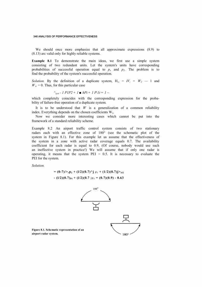
346 ANALYSIS OF PERFORMANCE EFFECTIVENESS
We should once more emphasize that all approximate expressions (8.9) to (8.13) arc valid only for highly reliable systems.
Example 8.1 To demonstrate the main ideas, we first use a simple system consisting of two redundant units. Let the system's units have corresponding probabilities of successful operation equal to px and p2. The problem is to find the probability of the system's successful operation.
Solution. By the definition of a duplicate system, H,, = IV, = W2 — 1 and W n = 0. Thus, for this particular case
^syst - 1 P1P2 + 1 ■ hPi + 1 P\1t = 1 ~ which completely coincides with the corresponding expression for the proba- bility of failure-free operation of a duplicate system.
It is to be understood that W is a generalization of a common reliability index. Everything depends on the chosen coefficients Wx.
Now we consider more interesting cases which cannot be put into the framework of a standard reliability scheme.
Example 8.2 An airport traffic control system consists of two stationary radars each with an effective zone of 180° (see the schematic plot of the system in Figure 8.1). For this example let us assume that the effectiveness of the system in a zone with active radar coverage equals 0.7. The availability coefficient for each radar is equal to 0.9, (Of course, nobody would use such an ineffective system in practice!) We will assume that if only one radar is operating, it means that the system PEI = 0.5. It is necessary to evaluate the PEI for the system.
Solution.
= (0-7)/>rp2 + (l/2)(0.7)^j p 2 + (1/2)(0.7)j> i42
- (l/2)(0.7)Pl + (l/2)(0.7 )p 2 = (0.7)(0.9) - 0.63
Figure 8.1. Schcmatic representation of an airport radar system.
180°
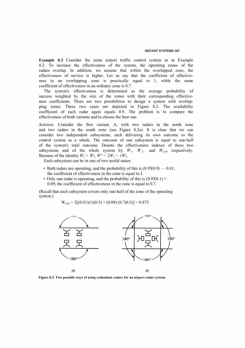
INSTANT SYSTEMS 347
Example 8.3 Consider the same airport traffic control system as in Example 8.2. To increase the effectiveness of the system, the operating zones of the radars overlap. In addition, we assume that within the overlapped zone, the effectiveness of service is higher. Let us say that the coefficient of effective- ness in an overlapping zone is practically equal to 1, while the same coefficient of effectiveness in an ordinary zone is 0.7.
The system's effectiveness is determined as the average probability of success weighted by the size of the zones with their corresponding effective- ness coefficients. There are two possibilities to design a system with overlap- ping zones. These two cases are depicted in Figure 8.2. The availability coefficient of each radar again equals 0.9. The problem is to compare the effectiveness of both variants and to choose the best one.
Solution. Consider the first variant, A, with two radars in the north zone and two radars in the south zone (see Figure 8.2a). It is clear that we can consider two independent subsystems, each delivering its own outcomc to the control system as a whole. The outcome of one subsystem is equal to one-half of the system's total outcome. Denote the effectiveness indexes of these two subsystems and of the whole system by W u W 2 , and Wiystt respectively. Because of the identity Wx = W2, W^ = 2Wx = 1W2.
Each subsystem can be in one of two useful states:
• Both radars are operating, and the probability of this is (0.9X0.9) — 0.81; the coefficient of effectiveness in the zone is equal to J.
• Only one radar is operating, and the probability of this is (0.9X0.1) = 0.09; the coefficient of effectiveness in the zone is equal to 0.7.
(Recall that each subsystem covers only one-half of the zone of the operating system.)
Wsyst = 2[(0.81)(1)(0.5) + (0.09) (0.7)0.5)] = 0.873
180s- 180°
(a) (b)
Figure 8.2. Two possible ways of using redundant radars for an airport radar system.
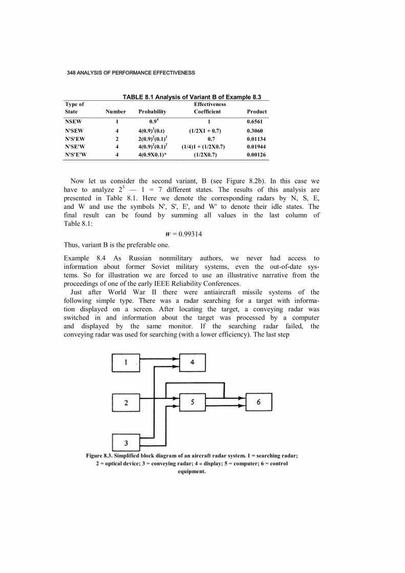
348 ANALYSIS OF PERFORMANCE EFFECTIVENESS
Now let us consider the second variant, B (see Figure 8.2b). In this case we have to analyze 23 — 1 = 7 different states. The results of this analysis are presented in Table 8.1. Here we denote the corresponding radars by N, S, E, and W and use the symbols N', S', E', and W' to denote their idle states. The final result can be found by summing all values in the last column of Table 8.1:
W = 0.99314 Thus, variant B is the preferable one.
Example 8.4 As Russian nonmilitary authors, we never had access to information about former Soviet military systems, even the out-of-date sys- tems. So for illustration we are forced to use an illustrative narrative from the proceedings of one of the early IEEE Reliability Conferences.
Just after World War II there were antiaircraft missile systems of the following simple type. There was a radar searching for a target with informa- tion displayed on a screen. After locating the target, a conveying radar was switched in and information about the target was processed by a computer and displayed by the same monitor. If the searching radar failed, the conveying radar was used for searching (with a lower efficiency). The last step
TABLE 8.1 Analysis of Variant B of Example 8.3 Type of Effectiveness
State Number Probability Coefficient Product
NSEW 1 0.94 1 0.6561 N'SEW 4 4(0.9)3(0.t) (1/2X1 + 0.7) 0.3060 N'S'EW 2 2(0.9)2(0.1)2 0.7 0.01134 N'SE'W 4 4(0.9)2(0.1)2 (1/4)1 + (1/2X0.7) 0.01944 N'S'E'W 4 4(0.9X0.1)* (1/2X0.7) 0.00126
Figure 8.3. Simplified block diagram of an aircraft radar system. 1 = searching radar; 2 = optical device; 3 = conveying radar; 4 « display; 5 = computer; 6 = control
equipment.
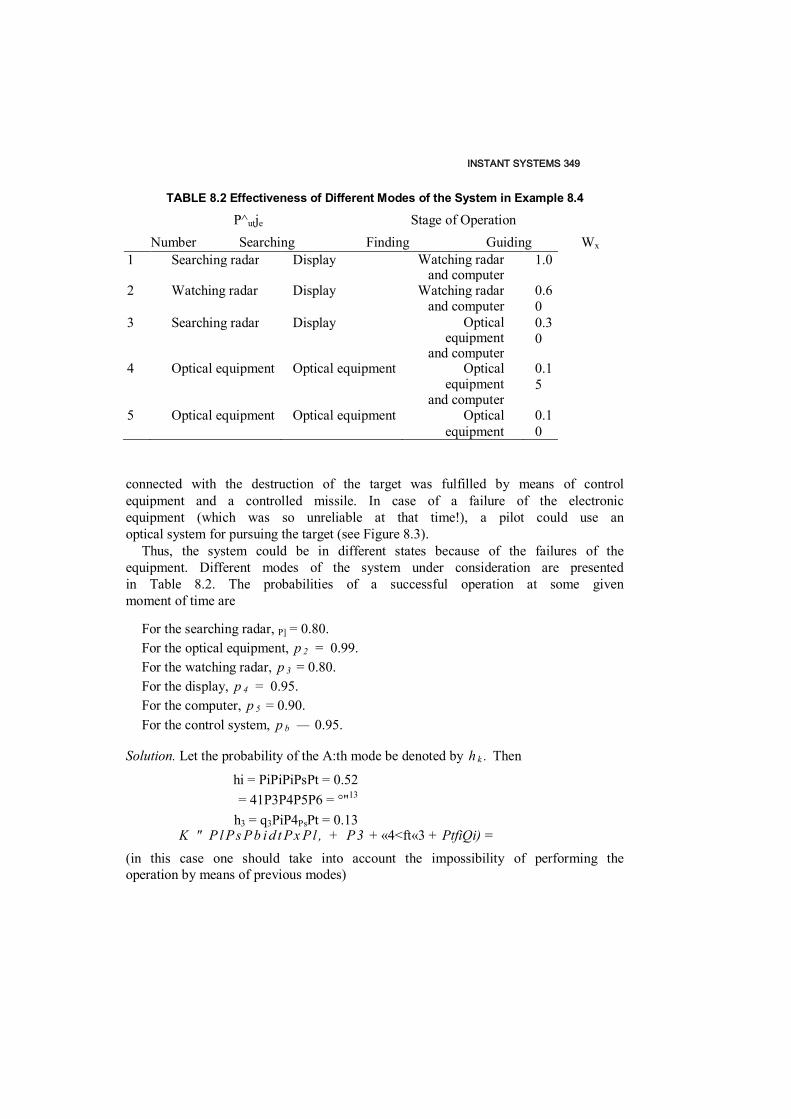
INSTANT SYSTEMS 349
connected with the destruction of the target was fulfilled by means of control equipment and a controlled missile. In case of a failure of the electronic equipment (which was so unreliable at that time!), a pilot could use an optical system for pursuing the target (see Figure 8.3).
Thus, the system could be in different states because of the failures of the equipment. Different modes of the system under consideration are presented in Table 8.2. The probabilities of a successful operation at some given moment of time are
For the searching radar, P] = 0.80. For the optical equipment, p 2 = 0.99. For the watching radar, p 3 = 0.80. For the display, p 4 = 0.95. For the computer, p 5 = 0.90. For the control system, p b — 0.95.
Solution. Let the probability of the A:th mode be denoted by h k . Then
hi = PiPiPiPsPt = 0.52 = 41P3P4P5P6 = °"13
h3 = q3PiP4PsPt = 0.13 K " P l Ps Pb i d t Px Pl , + P3 + «4<ft«3 + PtfiQi) =
(in this case one should take into account the impossibility of performing the operation by means of previous modes)
TABLE 8.2 Effectiveness of Different Modes of the System in Example 8.4
P^utje Stage of Operation
Number Searching Finding Guiding Wx 1 Searching radar Display Watching radar
and computer 1.0
2 Watching radar Display Watching radar and computer
0.60
3 Searching radar Display Optical equipment
and computer
0.30
4 Optical equipment Optical equipment Optical equipment
and computer
0.15
5 Optical equipment Optical equipment Optical equipment
0.10
350 ANALYSIS OF PERFORMANCE EFFECTIVENESS
a5 = p2QsPi(i4 + p*Q 1^3)11 °-12The final result is
that the probability of success is equal to
Wsyst = (0.51) ■ 1 + (0.13)(0.6) 4- (0.13)(0.3)
+ (0.08)(0.15) + (0.01)(0.1) - 0.66
12
max <7,(r,r + f0) « - (8.15) l s i i n n
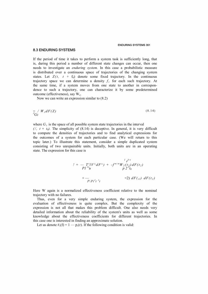
ENDURING SYSTEMS 351 8.3 ENDURING SYSTEMS
If the period of time it takes to perform a system task is sufficiently long, that is, during this period a number of different state changes can occur, then one needs to investigate an enduring system. In this case a probabilistic measure is distributed over a continuous space of trajectories of the changing system states. Let Z ( t , t + f0) denote some fixed trajectory. In the continuous trajectory space we can determine a density f z for each such trajectory. At the same time, if a system moves from one state to another in correspon- dence to such a trajectory, one can characterize it by some predetermined outcome (effectiveness), say Wz.
Now we can write an expression similar to (8.2)
= / W z d F( Z ) JGz
where G z is the space of all possible system state trajectories in the interval ( / , t + t0). The simplicity of (8.14) is deceptive. In general, it is very difficult to compute the densities of trajectories and to find analytical expressions for the outcomes of a system for each particular case. (We will return to this topic later.) To illustrate this statement, consider a simple duplicated system consisting of two unrepairable units. Initially, both units are in an operating state. The expression for this case is
1 rl+t ! + — T ' l V ^ d F^ ) + - f " ' "W 2 ( t 2 ) d F( t 2 )
P1 J'u p 2 Jt0
+ — <2) d F( t l ) d F( t 2 ) P\ Pi J t J t
Here W again is a normalized effectiveness coefficient relative to the nominal trajectory with no failures.
Thus, even for a very simple enduring system, the expression for the evaluation of effectiveness is quite complex. But the complexity of the expression is not all that makes this problem difficult. One also needs very detailed information about the reliability of the system's units as well as some knowledge about the effectiveness coefficients for different trajectories. In this case one is interested in finding an approximate solution.
Let us denote #,(f) = 1 — p,(r). If the following condition is valid:
(8 .14)
352 ANALYSIS OF PERFORMANCE EFFECTIVENESS
it is possible to write an
approximate formula for
unrepairable systems:
1 _ ^syst ~ "0 1
For repairable systems such an analysis becomes extremely difficult and boring. For numerical calculations one can introduce a discrete lattice to describe the system's trajectory in the space of system states. But in this case one encounters a complex factorial problem. Of course, the largest practical difficulties arise in the determination of the effectiveness coefficients for different state trajectories in both cases: continuous and discrete.
For enduring systems B^, is also a generalized index in comparison with the standard reliability indexes. As usual, a generalized (or more or less universal) method permits one to obtain any different particular solutions but with more effort. So, for simple reliability problems, one need not use this general approach. At the same time we should mention (hat, in general, a system performance effectiveness analysis cannot be done via common relia- bility methods.
We first consider two simple examples which can be solved by the use of standard reliability methods.
Example 8.5 Consider a unit operating in the time interval [0, Z ] . An outcome of the unit is proportional to the operating time; that is, if a random TTF is more than Z, then the outcome of the unit is proportional to Z, Let p i t ) be the probability of a failure-free operation during time t and let q i t ) — 1 — pit). Find an effectiveness index H<,yst.
Solution. Simply reformulating the verbal description gives the result
W ^ = Z p i Z ) + j Z t d q i t )
and, after integrating by parts,
- Z p ( Z ) + Z q i Z ) - f Z q ( t ) d t - Z - ( Z q ( t ) d t = f Z p ( t ) d t
As one can see (and as would be expected), the result coincides with the conditional MTTF inside the interval [0, Z].
E L ( t , t + t Q ) ~ r " ' W l ( x t ) d F i ( x , ) <i<n V ' J
ENDURING SYSTEMS 353
Example 8.6 Consider a system consisting of n identical and independent units. The system's behavior can be described with the help of the birth and death process (BDP). The effectiveness of the system during the time interval [(,/ + fD] is completely determined by the lowest state which the system attains. If the system's lowest state is k, denote the effectiveness coefficient by W k (see Figure 8.4), The problem is to determine B'
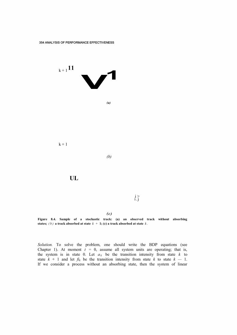
354 ANALYSIS OF PERFORMANCE EFFECTIVENESS
V1 (a)
k + 1
(b)
UL
i > i . j
(c) Figure 8.4. Sample of a stochastic track: (a) an observed track without absorbing states; ( b ) a track absorbed at state k + 1; (c) a track absorbed at state k .
Solution. To solve the problem, one should write the BDP equations (see Chapter 1). At moment t = 0, assume all system units are operating; that is, the system is in state 0. Let a k be the transition intensity from state k to state k + 1 and let fik be the transition intensity from state k to state k — 1. If we consider a process without an absorbing state, then the system of linear
k + 111
ENDURING SYSTEMS 355
differential equations is
( a k + P k ) R k ( t ) + 0 + J8 k + i R k + l ( t )
for 0 < k < n , a n + ] = = 0 (8.16)
and the initial condition is /?0(0) = 1. To solve the problem, we should solve (8.16) n times for different absorb- ing states. Namely, we should solve n subproblems of type (8.16) for absorb- ing states n , n - 1,..., 1. Let /?*(f) denote the probability that the process is in the absorbing state when the process is "cut" up to the absorbing state k (see Figure 8.4). From (8.16) it is clear that R*U) differs from R k ( t ) . Moreover, the sum of the /?*(0's over all k does not equal 1. We can use the methods described in Chapter 1. But our purpose is not to actually find the above-mentioned probabilities. For further consideration of this particular example, let us assume that we know the probabilities R % ( t ) which are the probabilities of reaching an absorbing state k in the corre- sponding subproblem (8.16). It is clear that if state k is absorbing, R * ( t ) is the probability that in the original state space the process would also reach states with larger subscripts. This means that
R W) = L s k ( t ) k z j z n
where S k ( t ) is the probability that the worst state that the initial process reached in [0, t ] is k . Hence, S k ( t ) = /?£(/) - /?*+,('). The final result is the following:
£ w k s k { t ) 0 sksn
Example 8.7 Consider a system that involves the collection and transmission of information. The system consists of two identical and independent com- munication channels. If a channel fails, the system capacity decreases to 0.3 times a nominal value. For simplicity, assume that each channel is character- ized by an exponentially distributed TTF with parameter A. Let the duration of a given information collection equal (0.1)/A. The volume of the collected
d t
356 ANALYSIS OF PERFORMANCE EFFECTIVENESS
information is proportional to the operating time, that is,
W 0 = t
W } ( x ) = W 2 { x ) = * + (0.3)(f ~ x ) = (0.3)f + (0.7)or
W ] 2 ( x l t x 2 ) = min(x l t J C 2) + 0.3[max( J C , , x 2 ) - min( x i , J C 2 ) ]
= 0.3 max(jci? jc2) + (0.7) min( , x 2 ) The task is to calculate expressed via the absolute amount of collected information.
Solution. In this case (8.14) can be written in the form
W m t C O - P2* + 2 p f ' ( 0 . 3 ) t + (Q.7)x\e-*X dx o
where we have denoted p = p i t ) = e A', After substituting the input data p = 0.905 and t = 1/A, one obtains the final result
Wsyst = (0.819 + 0.109 + 0.002)(1/A) m 0.94(1/A)
This value is the amount of information collected by the system as a whole during a time equal to the MTTF of a single channel.
8.4 PARTICULAR CASES
Below we consider several particular cases for which one can obtain simple results. Such kinds of structures are often encountered in practice.
8.4.1 Additive Type of a System Unit's Outcome We first consider an instantaneous system containing n independent units. Each of them performs its own task, which implements a determined portion Wi of the total system outcome. Therefore, the system's outcome H-'syst can be represented as the sum of the W - s. Each unit i can be in one of two states: successfully operating or failure, with probabilities Pi and q,, respectively. For such a system W , ' can be written as
= E WIPI t <.i<,n
Expression (8.17) can also be written for dependent units. This follows from
(8.17)
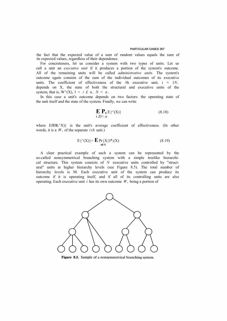
PARTICULAR CASES 357 the fact that the expected value of a sum of random values equals the sum of its expected values, regardless of their dependence.
For concreteness, let us consider a system with two types of units. Let us call a unit an executive unit if it produces a portion of the system's outcome. All of the remaining units will be called administrative units. The system's outcome again consists of the sum of the individual outcomes of its executive units. The coefficient of effectiveness of the /th executive unit, i = 1N , depends on X, the state of both the structural and executive units of the system, that is, W^(X), 1 < i £ n , N < n .
In this case a unit's outcome depends on two factors: the operating state of the unit itself and the state of the system. Finally, we can write
E P, E{^(X)} (8.18) i Zi<.n
where EfHK^X)} is the unit's average coefficient of effectiveness. (In other words, it is a W t of the separate i t h unit.)
E{^(X)}= E Pr{X}f*;(X) (8.19) all X
A clear practical example of such a system can be represented by the so-called nonsymmetrical branching system with a simple treelike hierarchi- cal structure. This system consists of N executive units controlled by "struct- ural" units at higher hierarchy levels (see Figure 8.5). The total number of hierarchy levels is M. Each executive unit of the system can produce its outcome if it is operating itself, and if all of its controlling units are also operating. Each executive unit i has its own outcome W t being a portion of
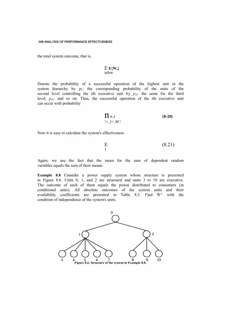
358 ANALYSIS OF PERFORMANCE EFFECTIVENESS
the total system outcome, that is,
E E{W,} isfsw
Denote the probability of a successful operation of the highest unit in the system hierarchy by p}; the corresponding probability of the units of the second level controlling the ith executive unit by p2i; the same for the third level, p3i; and so on. Thus, the successful operation of the ith executive unit can occur with probability
n P , J (8-20) \<.}<.M-\
Now it is easy to calculate the system's effectiveness
E (8.21) 1
Again, we use the fact that the mean for the sum of dependent random variables equals the sum of their means.
Example 8.8 Consider a power supply system whose structure is presented in Figure 8.6. Units 0, 1, and 2 are structural and units 3 to 10 are executive. The outcome of each of them equals the power distributed to consumers (in conditional units). All absolute outcomes of the system units and their availability coefficients are presented in Table 8.3. Find W^ with the condition of independence of the system's units.
0
Figure 8.6. Structure of the system in Example 8.8.
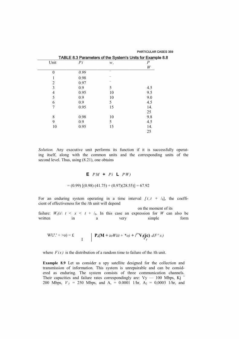
PARTICULAR CASES 359
Solution. Any executive unit performs its function if it is successfully operat- ing itself, along with the common units and the corresponding units of the second level. Thus, using (8.21), one obtains
E PM + P i L PW )
= (0.99) [(0.98) (41.75) + (0.97)(28.55)] = 67.92
For an enduring system operating in a time interval [ t , t + /0], the coeffi- cient of effectiveness for the /th unit will depend
on the moment of its failure: W((x\ t < x < t + /0. In this case an expression for W can also be written in a very simple form
WU'.' + >o) = £
I P,(M + toWiit + *o) + //+Vf(jc) d F^ x )
* t
where F i x ) is the distribution of a random time to failure of the /th unit.
Example 8.9 Let us consider a spy satellite designed for the collection and transmission of information. This system is unrepairable and can be consid- ered as enduring. The system consists of three communication channels. Their capacities and failure rates correspondingly are: Vy — 100 Mbps, Kj =
200 Mbps, V 3 = 250 Mbps, and A, = 0.0001 1/hr, A2 = 0,0003 1/hr, and
TABLE 8.3 Parameters of the System's Units for Example 8.8 Unit Pi w , P
W 0 0.99 —
1 0.98 —
2 0.97 —
3 0.9 5 4.5 4 0.95 10 9.5 5 0.9 10 9.0 6 0.9 5 4.5 7 0.95 15 14.
25 8 0.98 10 9.8 9 0.9 5 4.5 10 0.95 15 14.
25

360 ANALYSIS OF PERFORMANCE EFFECTIVENESS
A3 = 0.0004 1/hr. Find Wsyst (in absolute value) in two forms: (a) the mean capacity of the system as a whole at moment t - 1000, and (b) the mean volume of transmitted information during 5000 hours.
PARTICULAR CASES 361
Solution, (a) For an arbitrary moment t one can write
= E I S I S 3
After the substitution of numerical input data
1000) - 100e~°'! + 200e"03 + 250e"°-4 = 405.5 Mbps
(b) If, during the period [0, f„] in this example, there was no failure, a channel has collected H b i t s of information. If a failure has occurred at the moment t < t a , then a channel has collected Wtt bits of information. Taking this into account, one can write
W
- ™ [ l - e~x>'o} A;
Note that, since the amount of transmitted information is proportional to t 0 , the total operating time is
Substituting the input data (in the same time dimension), one obtains
Iflj, (0,5000)
100 200
250 -0.39 + _______ 0.78 +_________0.86 0.00003
8.4.2 Systems with a Symmetrical Branching Structure Now we consider a system whose structure presents a particular case of the system structure discussed in Example 8.8. The branching structure has a symmetry, which means that each controlling unit controls the same number of units in the lower level. Also, all units of the same hierarchical level have the same reliability characteristics; that is, the system is homogeneous.
»U(0,/o)- E ' n
3600 = 5.2 • I0y Mbits0.00001 0.00004

362 ANALYSIS OF PERFORMANCE EFFECTIVENESS
Now we will consider a more complex measure of system effectiveness: one that depends in a nonlinear way on the number of executive units performing their functions successfully.
The successful performance of a unit of any hierarchy level means that the unit is in an operating state and all of its controlling units are also in
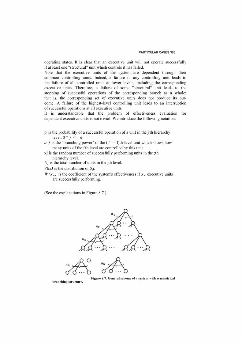
PARTICULAR CASES 363
operating states. It is clear that an executive unit will not operate successfully if at least one "structural" unit which controls it has failed. Note that the executive units of the system are dependent through their common controlling units. Indeed, a failure of any controlling unit leads to the failure of all controlled units at lower levels, including the corresponding executive units. Therefore, a failure of some "structural" unit leads to the stopping of successful operations of the corresponding branch as a whole; that is, the corresponding set of executive units does not produce its out- come. A failure of the highest-level controlling unit leads to an interruption of successful operations at all executive units. It is understandable that the problem of effectiveness evaluation for dependent executive units is not trivial. We introduce the following notation:
p; is the probability of a successful operation of a unit in the j'th hierarchy level, 0 ^ j < , n .
a j is the "branching power" of the (;" — l)th-level unit which shows how many units of the ;'th level are controlled by this unit.
xj is the random number of successfully performing units in the ;th hierarchy level.
Nj is the total number of units in the jth level. PfixJ is the distribution of Xj. W ( x n ) is the coefficient of the system's effectiveness if x n executive units
are successfully performing.
(See the explanations in Figure 8.7.)
Figure 8.7. General scheme of a system with symmetrical branching structure.
364 ANALYSIS OF PERFORMANCE EFFECTIVENESS
REMARK. Here we use the two expressions: "successfully operating" and "successfully per- forming." Really these expressions have a very slight difference. In this text we will understand that "operating" means that a unit is in an up state itself, independent of the states of any other unit in the system, and "performing" means that the unit is operating itself and, at the same time, ail of its controlling units are successfully operating. (See the explanations in Figure 8.7.)
For the system under consideration,
W W = Z Pn { x n ) W { x n ) = E { W (x n ) } (8.22)
where J V„ is the total number of the executive units:
K = 11 (8-23) t i i S r t
In general, the function W ( x n ) can be arbitrary. For simplicity, let us suppose that W { x ) is a continuous differentiate function of x . It is known that any such function can be represented in the form of a Taylor series. In the case under consideration,
„ , d k W ( x n ) n * n ) = Z < d t x (8.24)
t i l
For practical purposes, one can use an approximation taking (8.24) with relatively smalt k . Using (8.24), we can easily write
KY, - E{ Z - Z Bk E{xk„} = Z BkMk (8.25) Ui l ' Aa l A kl
where M k is the moment of the distribution of the number of successfully performing executive units. To find M k , we write the moment generating function. First, consider a group of executive units depending on a single unit in the (n — l)th level. We have Nn _, such groups. A random number of successfully operating execu- tive units in a group, x , has a binomial distribution B(an,pn). The moment generating function for the distribution of successfully operating executive units of the above-mentioned group is denoted by
g(e*~) - [ p n e x » + qn}"" (8-26)
Now consider all executive units which depend on Nn„x controlling units at the (n - l)th level. (At this stage of consideration we are not interested in all
PARTICULAR CASES 365
of the remaining units in the system.) The random number of successfully operating units at this level, x n , also has a binomial distribution
pM_,X Note that if no units at the (n - l)th level are successfully operating, no units at the nth level are successfully performing, even though all executive units are operating. This event occurs with probability:
^n-i(O) = In-V
If only one unit at the (n - l)th level is operating successfully, then not more than a n executive units can perform successfully. The random number of successfully performing executive units will have a binomial distribution with moment generating function (8.26). This event occurs with probability
^ - . ( ^ - ( ^ - ' j p - i f l ^ T ' - 1
If two units at the (n - l)th level are operating successfully then not more than 2"n executive units can perform successfully. The probability of this event equals P „ _ ,(2) where
Arguing in the same manner, we obtain the moment generating function of the distribution of the random number of all successfully performing execu- tive units, x,„ taking into account the random number of successfully operat- ing units at the (n - l)th level as a whole:
G n ( e x " ) = £ Pn - ^ . ^ g i e ^ " (8.27)
If we let
e ( Y) - G ( t ' " ) - [ p „e ' ' + q„]a"
(8-28
)
then (8.27) can be rewritten as
<*(«'•)- E Pn-\(xn-\)\eY\ " 1 ~ G „_ l ( e Y ) (8.29)
From (8.28) it follows that
(8.30)

366 ANALYSIS OF PERFORMANCE EFFECTIVENESS
Y^ a n ln( p„ex" + q n )
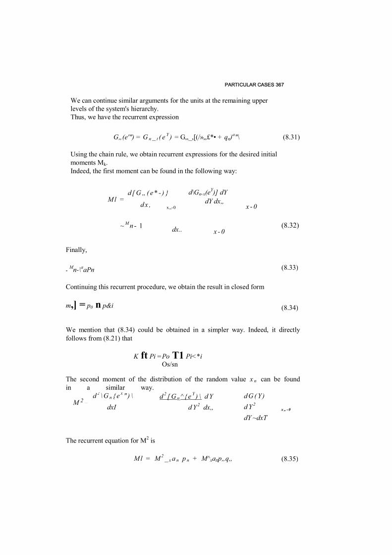
PARTICULAR CASES 367
We can continue similar arguments for the units at the remaining upper levels of the system's hierarchy. Thus, we have the recurrent expression
G„(e'") = G n _ t ( e Y ) = G„_,[(/»„£*• + qn)a"\ (8.31)
Using the chain rule, we obtain recurrent expressions for the desired initial moments Mk. Indeed, the first moment can be found in the following way:
d\Gn.x(eY)] dY
dY dx„
~ M n - 1
Finally,
= Mn-\aaPn
Continuing this recurrent procedure, we obtain the result in closed form
m,] = p0 n p&i
We mention that (8.34) could be obtained in a simpler way. Indeed, it directly follows from (8.21) that
K ft Pi =Po T1 Pi<*i Os/sn
The second moment of the distribution of the random value x n can be found in a similar way.
The recurrent equation for M2 is
M l = M 2 _ x a n p n + M^xattp„q„
d [ G „( e * - ) }
M l = d x , x„-0 x - 0
(8.32)dx.. x - 0
(8.33)
(8.34)
d 2 [ G n ^{ e Y ) \ d Y d Y 2 dx„
d G ( Y) d Y 2
dY ~dxT
d 2 \ G n { e x " ) \ 2 _ M dxI x „ - 0
(8.35)
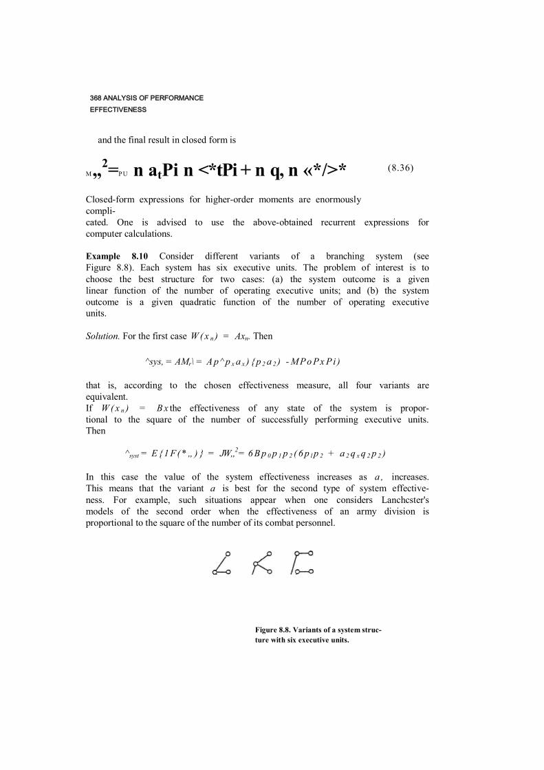
368 ANALYSIS OF PERFORMANCE EFFECTIVENESS
and the final result in closed form is
M„2=P U n atPi n <*tPi + n q, n «*/>* Closed-form expressions for higher-order moments are enormously compli- cated. One is advised to use the above-obtained recurrent expressions for computer calculations.
Example 8.10 Consider different variants of a branching system (see Figure 8.8). Each system has six executive units. The problem of interest is to choose the best structure for two cases: (a) the system outcome is a given linear function of the number of operating executive units; and (b) the system outcome is a given quadratic function of the number of operating executive units.
Solution. For the first case W ( x n ) = Axn. Then
^sys, = AMr\ = A p ^ p x a x ) { p 2 a 2 ) - M Po Px Pi )
that is, according to the chosen effectiveness measure, all four variants are equivalent. If W ( x n ) = B x the effectiveness of any state of the system is propor- tional to the square of the number of successfully performing executive units. Then
^syst = E { 1 F( * „) } = JW„2 = 6 B p 0 p 1 p 2 ( 6 p l p 2 + a 2 q x q 2 p 2 )
In this case the value of the system effectiveness increases as a , increases. This means that the variant a is best for the second type of system effective- ness. For example, such situations appear when one considers Lanchcster's models of the second order when the effectiveness of an army division is proportional to the square of the number of its combat personnel.
Figure 8.8. Variants of a system struc- ture with six executive units.
(8.36)
SYSTEMS WITH INTERSECTING ZONES OF ACTION 369
The system with the largest a z is the most effective. Thus, the higher the level of centralized control from the center, the better is the result.
8.4.3 Systems with Redundant Executive Units Many instant systems are used for fulfilling a given task. For example, an antiaircraft or antimissile defense system is designed to destruct a target. To improve the system's effectiveness, N redundant executive units can be used. If the system is in state X , each executive unit fulfills its task with probability Wt(X). For example, the efficiency of an antiaircraft missile system depends on the state of its subsystems which are used for searching, controlling, and so on. There are two main cases: (1) when all executive units perform their common task simultaneously (2) when units perform the same task sequen- tially.
Case 1 All units are dependent through the system state X. Then
»w- Enxjfi - n ( i - ^(x)) all X I l s i ^ N
In particular, for the branching system considered in the previous section, the problem can be solved in the following elegant way. Let D be the probability of success of a single executive unit (e.g., the kill probability of an enemy's aircraft). Then, if x n executive units are acting simultaneously, the total probability of success is
W ( x „) = 1 - ( 1 - D) x " (8.38)
An interesting particular case arises if we consider a symmetrical branching system. As discussed above, the effectiveness of the branching system is completely determined by the number of successfully performing executive units, xn. Thus, using (8.2), we can write
0^x„<N
= 1- L P( x n ) ( l - D) x "= 1-G„(i - D) (8.39) 0<.x„<.N
The second term in (8.39) is a moment generating function with the substitu- tion of 1 — D as a variable. Thus, (8.39) can be rewritten as
WW = 1 - G„(I - D ) - 1 - G„ _ , ( [ p„ ( l — £ > ) + q n ] " " ) (8.40)
(8.37)
370 ANALYSIS OF PERFORMANCE EFFECTIVENESS
+ ■•• + <?,)"' +<7o) (8.41)
Case 2 Assume that the system's executive units are operating sequentially. The system states are supposed to change between the use of two consequent executive units. If the time interval between the two system performances is large enough, the result of their operations might be independent. The same result will also be valid if one considers the simultaneous operation of several executive units controlled by identical and independent controlling systems. For example, one can consider the destruction of an enemy aircraft in the overlapping zone of action of several antiaircraft systems. In this case
= 1 - n 1 - E P(X)^(X) all x
8.5 SYSTEMS WITH INTERSECTING ZONES OF ACTION
8.5.1 General Description Suppose that a system consists of n executive units. Unit i has its own zone Z, of action. Each unit is characterized by its own effectiveness of action Wt in the zone Z(. These zones can be overlapping (see Figure 8.9).
The joint effectiveness of several executive units in such an overlapping zone depends on the types of systems and their tasks. Such systems appear in satellite intelligence systems, radio communication networks, power systems, and antiaircraft and antimissile systems (overlapping zones of destruction).
In general, in the entire zone in which a system as a whole is operating, 2" different overlapping subzones may be created. Then the problem of comput- ing the system's effectiveness cannot be reduced and we need to use a general expression:
^sys, = E HW
where H i is the probability that the system is in state i , W t is the conditional effectiveness performance index for this system state, and n is the total number of system units. Of course, the number 2" is huge if n > 10. Moreover, in a computational sense, for some hundreds of units the problem cannot be solved in general: there is not sufficient memory to store the data and there is not sufficient time to perform the computations!
+ •
(8.42)
Using a recurrent procedure, we finally obtain
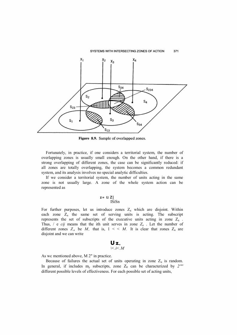
SYSTEMS WITH INTERSECTING ZONES OF ACTION 371
Fortunately, in practice, if one considers a territorial system, the number of overlapping zones is usually small enough. On the other hand, if there is a strong overlapping of different zones, the case can be significantly reduced: if all zones are totally overlapping, the system becomes a common redundant system, and its analysis involves no special analytic difficulties.
If we consider a territorial system, the number of units acting in the same zone is not usually large. A zone of the whole system action can be represented as
z= u Z| ISiSn
For further purposes, let us introduce zones Za which are disjoint. Within each zone Za the same set of serving units is acting. The subscript represents the set of subscripts of the executive units acting in zone Za . Thus, / e cij means that the ith unit serves in zone Za . Let the number of different zones Z a be M , that is, 1 < < M . It is clear that zones Za are disjoint and we can write
U z., \<.i<.M
As wc mentioned above, M 2" in practice. Because of failures the actual set of units operating in zone Zu is random.
In general, if includes my subscripts, zone Z0 can be characterized by 2'"' different possible levels of effectiveness. For each possible set of acting units,
372 ANALYSIS OF PERFORMANCE EFFECTIVENESS
say a]k , where kj ^ 2, we observe some specified coefficient of effectiveness Wa . As a result, for such a system we can write >ki
SYST= E 2fl) Z PkWa i k . (8.43)
Another, more compact representation of (8.43) is
SYST = E Z a E { W a j ) (8.44) \<.i<.M
Such a simple and obvious modification of the general expression (8.2) sometimes allows us to obtain constructive results for some important and interesting practical cases.
8.5.2 Additive Coefficient of Effectiveness In this case for any set of acting units in the zone we have
- E (8.45) I Gay
As an example, we can consider pollution in some region when each of several polluting companies makes its own "investment" in the total level of pollution. Pollution is assumed to be additive. (Of course, in this case it would be more reasonable to speak of loss rather than effectiveness.) It is clear that in this case for the system as a whole
E Wa j= Z P.ZW (8.46)
Let us illustrate this by a simple example.
Example 8.11 Consider a system consisting of two units and three acting zones (see Figure 8.10). Let us denote
Z \ = Z, 4- Z3 = the acting zone of the first unit. Z'2 = Z2 + Z3 = the acting zone of the second unit. Z3 = the acting zone of both units.
The effectiveness coefficient of the first unit is W{, and the effectiveness coefficient of the second unit is W2. By assumption of the additive character of the joint effect of the units, W3 = Wx + W2 for zone Z3.

SYSTEMS WITH INTERSECTING ZONES OF ACTION 373
Figure 8.10. Two overlapped zones.
Because all zones Z,, Z2, and Z3 are independent, we can write for the whole system
^ P \ Z \ W i + p 2 z 2 w 2 + z 3 [ p l p 2 ( i v 1 + w2) +a1p2w2+pig2w1]
= + Z 3 ) + p 2 W 2 ( Z 2 + Z 3 )
= P}W]Z\ +P2W2Z'2
8.5.3 Multiplicative Coefficient of Effectiveness In this case for any set of acting units in the zone we have
Wsysl WJ
It is more natural to consider a loss rather than a "positive" outcome. For example, 1 — Wj is the kill probability of a target in the acting zone of the ith unit of the system. Thus, if the ith unit does not act, this probability is 0. In other words, the probability of the enemy's survival (or, more accurately, the loss of the attacker) is IF, = 1. If a unit acts successfully, the enemy's damage is larger: the probability of the enemy's survival equals some Wi < 1. If in zone Z a units i„ i 2 , . . . , i k . act together successfully, then the probability of the enemy's survival is
W „ = W , W : « * * W , " i <! ' 2 ' t j
Taking into account the probability of success of the units, we can write
Wsyst= E !!(»">, + <?,) (8.47) 1

374 ANALYSIS OF PERFORMANCE EFFECTIVENESS
If we take into account that piWi + q, - 1 - p,w„ (8.47) can be rewritten as
E Za /nd -PVi) (8-48)
The final results (8.47) and (8.48) are illustrated by a simple example.
Example 8.12 The system under consideration is the same as in Example 8. 1 1 (see Figure 8.10 for an explanation). We use the same notation. To facilitate understanding, keep in mind the case of a target's destruction in the zone of defense. Thus, is the probability of failure of the ith executive unit, Pi = 1 — q,, and Wt is the probability of a target's destruction by the ith executive unit. Assume that the probability of a target's appearance in a zone is proportional to its size. Then the probability of the target passing through the defense zone equals
W ^ = Z x ( W x p x q x ) + Z 2 ( W 2 p 2 + q 2 ) + Z3(plp2WlW2 + P xq2wx + p 2 q x W 2 + q x q 2 )
= Z x ( W x P x + q x ) + Z 2 ( W 2 p 2 + q 2 ) + Z i ( p x W x + q x ) ( p2W2 + q 2 )
or, equivalently
^vm " 2,(1 - w ] P l ) + Z2( 1 ~ w 2 p 2 ) + Z 3 ( l ~ p , w, ) ( l ~ p 2 w 2 )
8.5.4 Redundant Coefficient of Effectiveness Now we consider a "positive" outcome in a zone. This type of effectiveness cocfiicient is, in cffect, complementary to the one considered in the previous section. For any set of acting units in the zone,
ww -1 - n "v where H>; = 1 — WT and WT has the previous meaning, that is, the probability of success. For this system we obtain
^Kyst E Zfl, 1
If we again take into account that piwi + qi = I - ptWh (8.50) can be rewritten as
i - no -PM )
I Z j s M
Again, let us illustrate the final result by a simple example.
(8.49)
i - n (piwi+<?,)
(8.50)
'syst E (8,51)
ASPECTS OF COMPLEX SYSTEMS DECOMPOSITION 375
Example 8.13 Consider again the system represented in Figure 8,10. Using the previous arguments, we have
w^zxpxwi+z2p2w2
+ Z3[p!p2( 1 - K> t w z ) + plq2Wl + p2qxw2\
- Z^ - O - p . wO ] + z 2 [ l - ( l - p 2 w 2 ) ]
+ Z3[l - (/?,iv, + q x ) { p 2 w 2 + q 2 ) ]
8.5.5 Boolean Coefficient of Effectiveness
This case is very close to ordinary redundancy applied to each zone. In other words, at least one executive unit must act in a zone to fulfill the operation within that zone. Thus, if a} is a set of units acting in the /th zone and unit i delivers the outcome W } in this zone, then any subset—a *, a * c a s and a* ¥= 0—delivers the same effectiveness Wr For example, if we consider a communication with a zone, it is sufficient to have at least one path of connection with this zone. For the system as a whole, we have
i- ru
i s a j
We assume that (8.52) does not demand any additional comments.
8.5.6 Preferable Maximal Coefficient of Effectiveness
If a set of units a* might act in the j"th zone, then for the actual operation the unit with the maximal possible effectiveness coefficient is chosen
W * = max W i (8.53)
Enumerate all of the system units in decreasing order of their effectiveness indexes IV,: W{ > W2 > • • • > Wn. Then in the /th zone the kth one uses the unit which is characterized by the effectiveness coefficient W k (of course, k e a f ) if and only if the ith unit itself is operational and there are no other operational units with i < k. This means that all units belonging to the set and having smaller numbers have failed at the moment of use. After this argument, it is simple to write the following expression:
- E Z0/ E Wk Pk ] I c h (8.54) \<.j<M Area. \<k
(8.52)
l& jsM

376 ANALYSIS OF PERFORMANCE EFFECTIVENESS
* i ^ a
ASPECTS OF COMPLEX SYSTEMS DECOMPOSITION 377
This follows directly from the formulation of the problem. We again think that there is no special need to explain it in more detail.
8.5.7 Preferable Minimal Coefficient of Effectiveness In this case, if a set of units a* might act in the jth zone, then for the actual operation the unit with the minimal possible effectiveness coefficient is chosen
W a = min W t
(8.55) ' i e a f
This kind of effectiveness coefficient can be chosen if one investigates damage rather than a "positive" outcome. Actually, this case is not distinguished from the previous one. One can even keep formula (8.54) with only one very essential difference: the enumer- ation of the system's executive units must be done in an increasing order of effectiveness indexes Wt: < IV2 < • • • < Wn.
8.6 ASPECTS OF COMPLEX SYSTEMS DECOMPOSITION
As mentioned above, the problem of effectiveness analysis arises in connec- tion with the analysis of complex systems. Thus, the more complex a system is, the more important and, at the same time, the more difficult is the evaluation of its effectiveness. Thus, the problem of simplifying the evalua- tion of effectiveness, in particular, the methods of decomposition, seems very important. Above we considered systems consisting of units with two states: an operating state and an idle state. But one sometimes deals with complex systems consisting of many such subsystems which themselves can be consid- ered as complex systems. This is equivalent to the consideration of a system consisting of units with more than two states. Let n be the total number of system units. Suppose the system is divided into M subsystems by some rule (it can be a functional principle or a constructive one). Each jth subsystem includes units and, consequently, has
nij = 2"' different states. Now the system consists of M new units, each with t r i j > 2 states. Of course, such a system representation does not lead to a decrease in the total number of system states m\ that is, it does not follow that

378 ANALYSIS OF PERFORMANCE EFFECTIVENESS
m = Yi 2"' £ 2" 1 sis M
But such a new system representation may still help to generate new ideas.
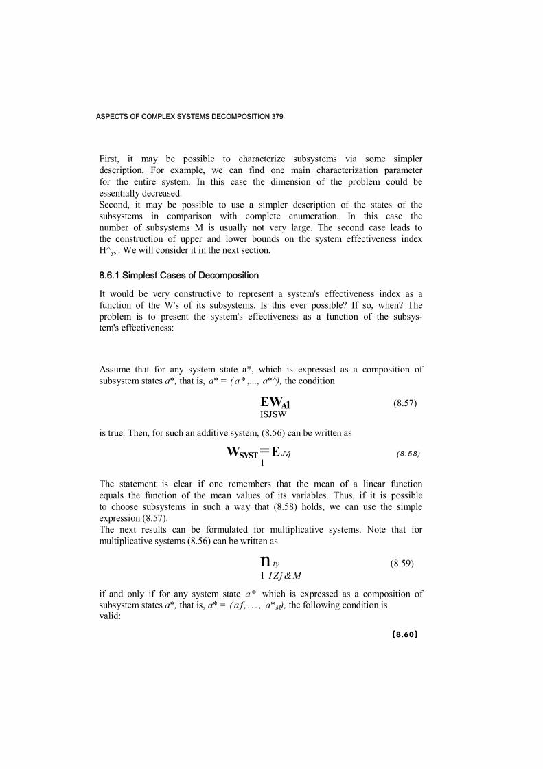
ASPECTS OF COMPLEX SYSTEMS DECOMPOSITION 379
First, it may be possible to characterize subsystems via some simpler description. For example, we can find one main characterization parameter for the entire system. In this case the dimension of the problem could be essentially decreased. Second, it may be possible to use a simpler description of the states of the subsystems in comparison with complete enumeration. In this case the number of subsystems M is usually not very large. The second case leads to the construction of upper and lower bounds on the system effectiveness index H^ysl. We will consider it in the next section.
8.6.1 Simplest Cases of Decomposition
It would be very constructive to represent a system's effectiveness index as a function of the W's of its subsystems. Is this ever possible? If so, when? The problem is to present the system's effectiveness as a function of the subsys- tem's effectiveness:
Assume that for any system state a*, which is expressed as a composition of subsystem states a*, that is, a* = ( a * ,..., a*^), the condition
E WA1 (8.57) ISJSW
is true. Then, for such an additive system, (8.56) can be written as
WSYST = E JVj (8 . 5 8) 1
The statement is clear if one remembers that the mean of a linear function equals the function of the mean values of its variables. Thus, if it is possible to choose subsystems in such a way that (8.58) holds, we can use the simple expression (8.57). The next results can be formulated for multiplicative systems. Note that for multiplicative systems (8.56) can be written as
n ty (8.59) 1 I Z j &M
if and only if for any system state a * which is expressed as a composition of subsystem states a*, that is, a* = ( a f , . . . , a*M), the following condition is valid:
(8.60)

380 ANALYSIS OF PERFORMANCE EFFECTIVENESS
n K* 1 ZJ ZM
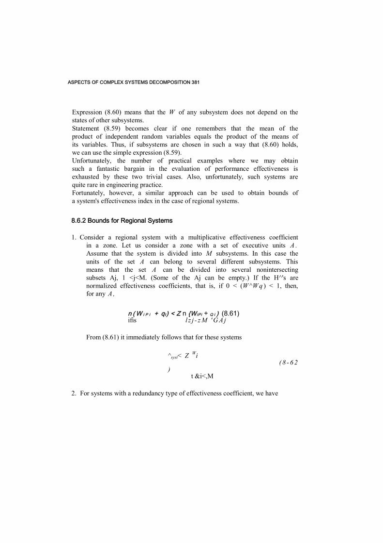
ASPECTS OF COMPLEX SYSTEMS DECOMPOSITION 381
Expression (8.60) means that the W of any subsystem does not depend on the states of other subsystems. Statement (8.59) becomes clear if one remembers that the mean of the product of independent random variables equals the product of the means of its variables. Thus, if subsystems are chosen in such a way that (8.60) holds, we can use the simple expression (8.59). Unfortunately, the number of practical examples where we may obtain such a fantastic bargain in the evaluation of performance effectiveness is exhausted by these two trivial cases. Also, unfortunately, such systems are quite rare in engineering practice. Fortunately, however, a similar approach can be used to obtain bounds of a system's effectiveness index in the case of regional systems.
8.6.2 Bounds for Regional Systems
1. Consider a regional system with a multiplicative effectiveness coefficient in a zone. Let us consider a zone with a set of executive units A . Assume that the system is divided into M subsystems. In this case the units of the set A can belong to several different subsystems. This means that the set A can be divided into several nonintersecting subsets Aj, 1 <j<M. (Some of the Aj can be empty.) If the H^'s are normalized effectiveness coefficients, that is, if 0 < (W ^W q ) < 1, then, for any A ,
n ( W i P i + qt) < Z n {W iPi + Q i ) (8.61) ifis l z j - z M ' G A j
From (8.61) it immediately follows that for these systems
^syst< Z Wi ( 8 - 6 2)
t &i<,M
2. For systems with a redundancy type of effectiveness coefficient, we have
382 ANALYSIS OF PERFORMANCE EFFECTIVENESS
^ s y s t < Z W , (8.63)
To confirm (8.63), we show that this is correct for a zone with two acting units belonging to different subsystems. Keeping in mind that 0 < Wi; < 1, i = 1,2, we can easily write
1 - ( p x w x + q l ) ( p 2 w 2 + q 2 ) < p x W y + p 2 W 2 (8.64)
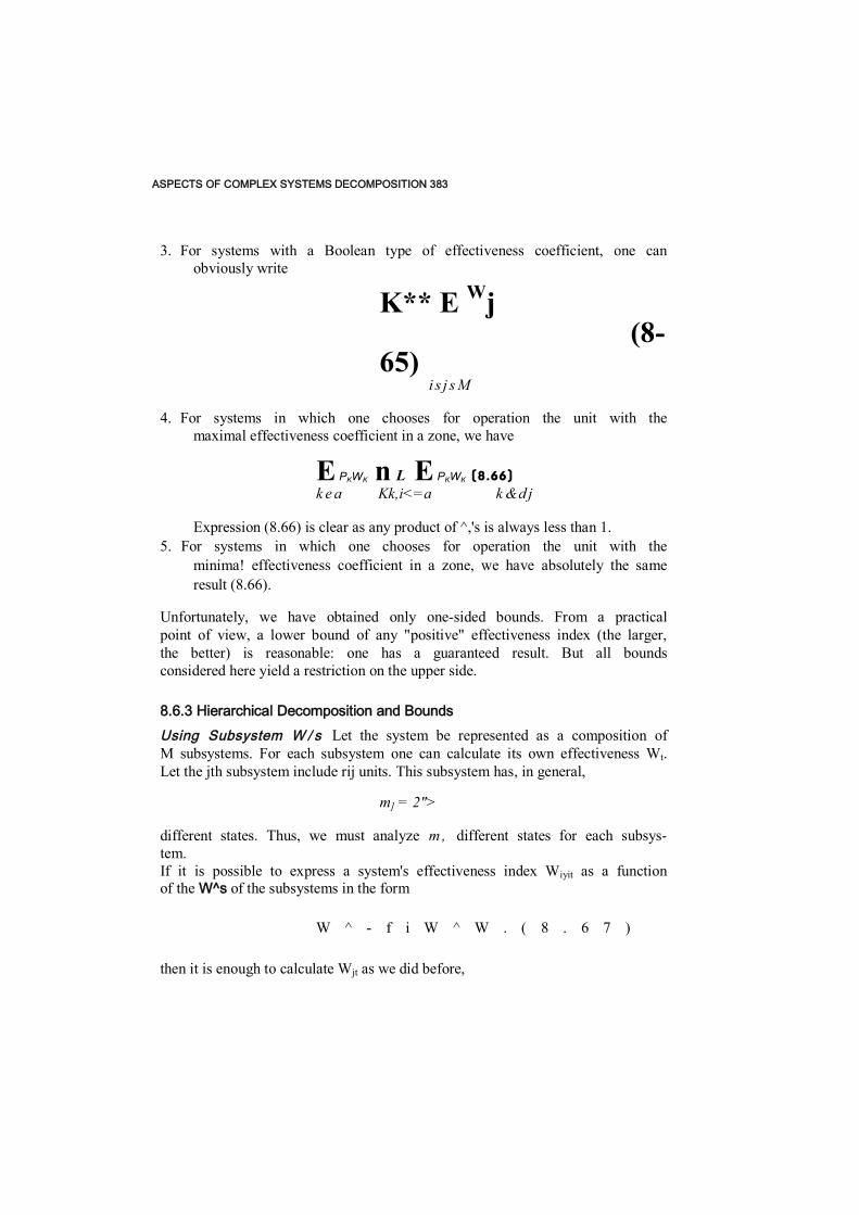
ASPECTS OF COMPLEX SYSTEMS DECOMPOSITION 383
3. For systems with a Boolean type of effectiveness coefficient, one can obviously write
K** E Wj (8-65)
i s j s M
4. For systems in which one chooses for operation the unit with the maximal effectiveness coefficient in a zone, we have
E PKWK n L E PKWK (8.66) k e a Kk,i<=a k &d j
Expression (8.66) is clear as any product of ^,'s is always less than 1. 5. For systems in which one chooses for operation the unit with the
minima! effectiveness coefficient in a zone, we have absolutely the same result (8.66).
Unfortunately, we have obtained only one-sided bounds. From a practical point of view, a lower bound of any "positive" effectiveness index (the larger, the better) is reasonable: one has a guaranteed result. But all bounds considered here yield a restriction on the upper side.
8.6.3 Hierarchical Decomposition and Bounds Using Subsystem W / s Let the system be represented as a composition of M subsystems. For each subsystem one can calculate its own effectiveness Wt. Let the jth subsystem include rij units. This subsystem has, in general,
m] = 2">
different states. Thus, we must analyze m , different states for each subsys- tem. If it is possible to express a system's effectiveness index Wiyit as a function of the W^s of the subsystems in the form
W ^ - f i W ^ W . ( 8 . 6 7 )
then it is enough to calculate Wjt as we did before,
384 ANALYSIS OF PERFORMANCE EFFECTIVENESS
V = E r{Xji}Wit
(8.68)
1 ^ i ^ m j
and, after this, use (8.67).

ASPECTS OF COMPLEX SYSTEMS DECOMPOSITION 385
The total number of computations to obtain the desired result is propor- tional to
£ 2m> « 2" (8.69) l -&j<,M
Unfortunately, such a procedure cannot be used too frequently as functions such as (8.67) are seldom known. The two simplest examples were shown above. At any rate, this method allows one to obtain at least some rough estimates of the unknown value of W^,.
Let us give several examples of the effectiveness of such a decomposition. For a system consisting of n — 400 units, a strict evaluation of the system's effectiveness is practically impossible because the number of all possible system states exceeds the so-called googol (lO100). As the reader may know, the googol is sometimes jokingly called "the greatest number in the universe." Indeed, everything in the universe—its maximal diameter, its time of exis- tence since the Big Bang, its total number of smallest elementary particles—measured by the smallest physical units (length or time, respec- tively) is smaller than this definitely restricted number. Thus, any attempt just to enumerate all the states of the above-mentioned system is unrealistic.
But if the system is divided into 20 subsystems, each consisting of 20 units, the number of calculations will still be large—20 ■ 2030 = 2 • 107—but at least it is a realistic number. If it is possible to divide the system into 40 subsystems, the corresponding number equals 40 * 2"' ~ 4 * 104, which is unconditionally acceptable.
REMARK. We mention that very complex systems are usually considered in engineering practice in a hierarchical way with more than two levels. This permits one to independently analyze first the system as a whole; then each subsystem as a part of the system, but performing its own functions; then some more-or-less autonomous parts of these subsystems; and so on. Such a mode is very effective in the evaluation of a system's effectiveness.
Let us again consider a system consisting of n = 400 units. Suppose the system is divided into 5 subsystems, each subsystem is divided into 5 au- tonomous parts, where each part consists of 16 units. Thus, the total number of calculations can be evaluated as the total number of parts in the system, multiplied by the number of calculations for one such part: 5 ■ 5 ■ (216) = 200,000. It is significantly less than in the initial case.
It is interesting to note that, for a system consisting of n = 1000 units, one can obtain an even smaller number of calculations if the system is repre-

386 ANALYSIS OF PERFORMANCE EFFECTIVENESS
sented by a three-level hierarchy: 5 subsystems, each of 5 parts, each of 5 complex units, each of 8 units of the lowest level. The number of calculations required is equal to 5 • 5 • 5 • (2a) = 32,000.

PRACTICAL RECOMMENDATION 387
Distributions of Subsystem Levels of W A more accurate method than the previous one is described next. From the viewpoint of a system's user, all subsystem states can be divided into a very restricted number of groups. The states of each such group are characterized by a value close to the value of the subsystem's effectiveness coefficient Wj. It is clear that the number of such groups could be very small, say 10. This number does not depend on the initial number of subsystem states. (One has also to take into account that there is no necessity to consider groups with levels of effectiveness which appear with an infinitesimally small probability and/or with levels of one essentially negligible effectiveness.)
At any rate, the first step in the analysis of a system's effectiveness consists in a detailed analysis of each subsystem. For each subsystem j, we need to analyze all possible states X1 < i < 2m'. Also, for each such subsystem we need to choose a reasonable lattice of the effectiveness coefficient values. Assume this lattice has Kj different cells:
• The first cell includes those states whose effectiveness coefficients Wt) satisfy the condition 1 = W^ < Wj < Bt, where B{ is the first threshold of the lattice; for all states belonging to this cell of the lattice, one computes the total probability R } as the sum of the probabilities of all states whose effectiveness values are included in this ccll.
• The second cell includes those states whose effectiveness coefficients Wtj satisfy the condition B x < W j < B 2 , where B 2 is the second threshold of the lattice; the corresponding probability computed is R2.
• The Kjth cell includes those states whose effectiveness coefficients W{J satisfy the condition B { K } — 1) < W j < 0, where B K is the last thresh- old of the lattice; the corresponding probability computed is R K f ,
We may now analyze the system as a whole. In each cell of the lattice, we choose a "middle" state which corresponds to the average value of Wj. For future analysis, this state now becomes a "representative" of all of the remaining states related to this cell. Thus, we choose K ; representatives for each subsystem. We should choose an appropriate number of representa- tives, say X * . Each of them appears with probability R j r The number of representatives is determined with respect to the required accuracy of the analysis and the available computer capacity.
After these preliminary steps we consider
K- N (8 .70)
different system states and, for each of them, evaluate the effectiveness coefficient. We then consider all K system states

388 ANALYSIS OF PERFORMANCE EFFECTIVENESS
X = (Jf*; 1 < j < M ) = ( X * r X * r . . . , X * J

PRACTICAL RECOMMENDATION 389
and write the expression for Wsyst with the use of (8.62)
PK1= E W(Xth ............ Xt,J n il^l-**)0" (8.71) alt X
This expression is not too pleasant in visual form because of the notation used. Neither is it easy to compute. But its nature is simple and completely coincides with (8.61).
Of course, if we decide to distinguish several levels of a system's hierarchy, the methodology would be the same but the corresponding description, in a general form, would be even longer than (8.71). We would like to emphasize that a hierarchical model needs less computation.
This method of representative selection can be successfully used for obtaining lower and upper bounds,
1. Let us choose from among the states of the latticc cell a state with a minimal effectiveness coefficient and consider this state as a representa- tive of this cell. Denote this aggregate state by Xp™. If we substitute Ay1"" instead of X * in (8.71), we will obtain a lower bound for the system index,
2. If a state XJ"ax with a maximal effectiveness coefficient is chosen as the representative of the cells, then the same procedure gives us an upper bound for W^,3*.
Thus, we obtain two-sided bounds for W^,:
W™ < £ W™ (8.72)
In genera], for practical purposes, it is enough to have an approximate expression (8.71). We should emphasize that reliability (and also effectiveness performance) computations are usually provided not for a precise evaluation of different indexes, but usually for a comparison of competitive variants at some design stage. For such purposes, we may use an approximate solution as a direction for design.
8.7 PRACTICAL RECOMMENDATION
An analysis of the performance effectiveness of a system must be carried out by a researcher who deeply comprehends the system as a whole, knows its operation, and understands all demands on the system. It is a necessary condition of successful analysis. Of course, the systems analyst should also be acquainted with operations research methods. As with any operations re-

390 ANALYSIS OF PERFORMANCE EFFECTIVENESS
search problem, the task is concrete and its solution is more of an art than a science.

PRACTICAL RECOMMENDATION 391
For simplicity of discussion, we demonstrate the effectiveness analysis methodology referring to an instant system. The procedure of a system's effectiveness evaluation, roughly speaking, consists of the following tasks:
• A formulation of an understandable and clear goal of the system. • A determination of all possible system's tasks (operations, functions). • A choice of the most appropriate measure of system effectiveness. • A division of a complex system into subsystems. * A compilation of a structural-functional scheme of the system which reflects the interaction of the system's subsystems. ■ A collection of reliability data. * A computation of the probabilities of the different states in the system and its subsystems. * An estimation of the effectiveness coefficients of different states. * A performance of the final computations of the system's effectiveness.
Of course, the effectiveness analysis methodology of enduring systems is quite similar, with the exception of some terms.
We need to remark that the most difficult part of an effectiveness analysis is the evaluation of the coefficients of effectiveness for different system states, in only extremely rare cases is it possible to find these coefficients by means of analytical approaches. At any rate, in the initial stages of a system's design there is no other way. The most common method is to simulate the system with the help of a computerized model or a physical analogue of the system. In the latter case, the analyst introduces different failures at appropriate moments into the system and analyzes the consequences. The last and the most reliable method is to perform experiments with the real system or, at least, with a prototype of the system.
Of course, one has to realize that usually all of these experiments set up to evaluate effectiveness coefficients are very difficult and they demand much time, money, and other resources. Consequently, one has to consider how to perform only really necessary experiments. This means that a prior evalua- tion of different state probabilities is essential: there is no need to analyze extremely rare events.
One can see that the analysis of a system's effectiveness performance is not routine. Designing a mathematical model of a complex system is, in some sense, a problem similar to the problem of designing a system itself. Of

392 ANALYSIS OF PERFORMANCE EFFECTIVENESS
course, there are no technological difficulties—no time or expense for engineering design and production.
REFERENCES 393CONCLUSION
It seems that the first paper devoted to the problem discussed in this chapter was the paper by Kolmogorov (1945). This work focused on an effectiveness measure of antiaircraft fire. The total kill probability of an enemy's aircraft was investigated. The random nature of the destruction of different parts of an aircraft and the importance of these parts was assumed. It is clear that from a methodological viewpoint the problem of system effectiveness analysis is quite similar: one has only to change slightly the terminology.
The first papers concerning a system's effectiveness evaluation appeared in the early 1960s [see, e.g., Ushakov (1960, 1966, 1967)]. Some special cases of system effectiveness evaluation were considered in Ushakov (1985, 1994) and Netes (1980, 1984).
One can find an analysis of the effectiveness of symmetrical branching systems in Ushakov (1985, 1994) and Ushakov and'Konyonkov (1964). Terri- torial (regional) systems with intersecting zones of action were studied in Ushakov (1985, 1994). Here one can also find an analysis of decomposition methods. The general methodology and methods of system effectiveness analysis are described in Ushakov (1985, 1994).
REFERENCES
Kolmogorov, A. N. (1945). A number of target hits by several shots and general principles of effectiveness of gun-fire (in Russian). Proc. Moscow Inst. Math., Issue 12.
Netes, V. A. (1980). Expected value of effectiveness of discrete system (in Russian). Automat. Comput. Sci., no. 11.
Netes, V. A. (1984). Decomposition of complex systems for effectiveness evaluation. Engrg. Cybernet. (USA), vol. 22, no. 4.
Ushakov, I. A. (1960). An estimate of effectiveness of complex systems. In Reliability of Radioelectronic Equipment (in Russian). Moscow: Sovietskoye Radio.
Ushakov, I. A. (1966). Performance effectiveness of complex systems. In On Reliability of Complex Technical Systems (in Russian). Moscow: Sovietskoe Radio. Ushakov, I. A. (1967). On reliability of performance of hierarchical branching systems
with different executive units, Engrg. Cybernet. (USA), vol. 5, no. 5. Ushakov, I. A., ed. (1985). Reliability of Technical Systems: Handbook (in Russian).
Moscow: Radio i Sviaz. Ushakov, I. A., ed. (1994). Handbook of Reliability Engineering. New York: Wiley.
Ushakov, I. A., and Yu. K. Konyonkov (1964). Evaluation of effectiveness of complex branching systems with respect to their reliability. In Cybernetics in Service for
Communism (in Russian), A. Berg, N. Bruevich, and B, Gnedcnko, eds. Moscow: Nauka.
394 ANALYSIS OF PERFORMANCE EFFECTIVENESS
EXERCISES
8.1 A conveyor system consists of two lines, each producing N items per hour. Each of the lines has an availability coefficient K = 0.8. When one of the lines has failed, the other decreases its productivity to Q.7N because of some technological demands. There is a suggestion to replace this system with a new one consisting of one line with a productivity of I . I N items per hour and an availability coefficient Kt = 0,9. Is this replacement reasonable from an effective productivity viewpoint or not?
8.2 A branching system has one main unit and three executive ones. There are two possibilities: (1) to use a main unit with PFFO p 0 = 0.9 and an executive unit with PFFO = 0.8 or (2) to use a main unit with PFFO p 0 = 0.8 and an executive unit with PFFO p, = 0.9. Is there is a difference between these two variants if the system's effectiveness depends on (a) the average number of successfully operating executive units, (b) a successful operation at least one executive unit, and (c) a successful operation of all executive units?
SOLUTIONS
8.1 The old system of two lines has the following states:
- Both lines operate successfully. In this case the effective productivity of the system is 2 N. This state occurs with probability P = (0.8X0.8) - 0.64. • One line has failed and the other is operating. This state occurs with probability P = 2(0.8X0.2) = 0.32. During these periods the system productivity equals 0.7N. * Both lines have failed. This state occurs with probability P = (0.2X0.2) = 0.04. The system productivity obviously equals O.Thus, the total average productivity of the old system can be evaluated as
WM = (0.64)(2.0) + (0.32)(0.7) = 1.5
The new system has an average effective productivity equal to
H^w - (1.7) (0.9) - 1.53

SOLUTIONS 395
Thus, the average productivity of both systems is very close. The increase in productivity is about 1.5%. One has to solve this problem

396 ANALYSIS OF PERFORMANCE EFFECTIVENESS
taking into account expenses for installation of the new system, on the one hand, and the potential decrease in the cost of repair, on the other hand (the new system will fail less often). (a) The average number of successfully operating executive units de-
pends only on the product pnp,, so both systems are equivalent. (b) For (1) one has Wsyst = (0.9X1 - 0.8)3 « 0.898 and for (2) ^sys, =
(0.8X1 - 0.9)3 = 0.799. Thus, the first variant is more effective. (c) For (1) one has = (0.9X0.8)3 * 0.460 and for (2) Wsyst =
(O.SXO^)3 » 0.584. In this case the second variant is more effective.

CHAPTER 9
TWO-POLE NETWORKS
Above we considered systems with a so-called "reducible structure." These are series, parallel, and various kinds of mixtures of series and parallel connections. As mentioned, they are two-pole structures which can be reduced, with the help of a simple routine, into a single equivalent unit. However, not all systems can be described in such a simple way. We would like to emphasize that most existing networks, for example, communication and computer networks, transportation systems, gas and oil pipelines, electric power systems, and others, have a structure which cannot be described in terms of reducible structures, even if they are considered as two-pole networks.
340
Probabilistic Reliability Engineering. Boris Gnedenko and Igor Ushakov
Figure 9.1. Bridge structure.

398 TWO-POLE NETWORKS The simplest example of a system with a nonreducible structure is the so-called bridge structure (see Figure 9.1). This particular structure is proba- bly not of great practical importance, but it is reasonable to consider it in order to demonstrate the main methods of analysis of such kinds of struc- tures.
9.1 RIGID COMPUTATIONAL METHODS
9.1.1 Method of Direct Enumeration The bridge structure cannot be represented as a connection of parallel-series or series-parallel subsystems of independent units (links). For this system the structure function t p ( X ) , where X = ( * , , x 2 , x3, x 4 , J C 5), can be written in tabular form (see Table 9.1) where all possible system states and correspond- ing structure function values are presented.
Because each Boolean variable has two possible different values, 0 or 1, the system can be characterized by 2s = 32 different states. In Table 9.1 we enumerate all possible values of the variables x v x 2 , . . . , x 5 and denote them as X v X 2 , . . . , X32. Some A^'s are states of successful operation of the bridge system (the set G) and some of them are not (the set G). In this notation the structure function of the bridge system can be written as
< p ( x i , . . . , x 5 ) =< p ( X l ) U < p ( X 2 ) U< - - U < p( X 3 2 ) = U <P(**) (9.1)
The probability of a system's successful operation is
PT {< P ( X I , . . . , X 3 ) -1}-E{ U ?(**)}- L EM**)} (9.2) ^ X K E G ' X K M G
Each vector X k can be expressed through its component x's and x's. For example (see Table 9.1),
~ ( * 1 » X 2 > x s ) From Table 9.1 it follows that the vector X s belongs to G, and so it will be taken into account in (9.2). Then
< P( * S) = x x x 2 x 3 x A x 5 and
E{<K*s)} = E { X i X 2 x 3 x 4 x 5 ) = E{*,} E { X 2 ) E{X3} E{jc5} = Q T P 2 q 3 p A p s
We do not write the detailed expression for < p ( X ) here. This can be easily obtained from Table 9.1 by taking into account that the corresponding term
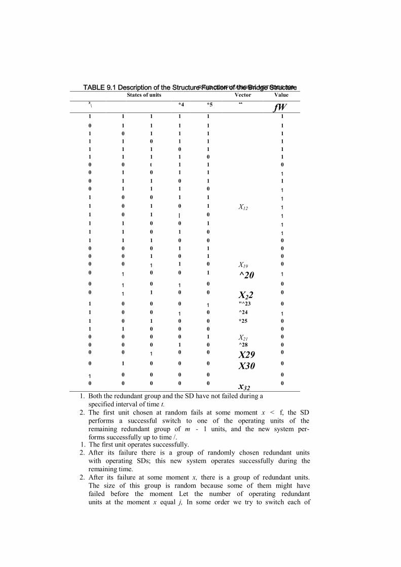
RIGID COMPUTATIONAL METHODS 399
1. Both the redundant group and the SD have not failed during a specified interval of time t.
2. The first unit chosen at random fails at some moment x < f, the SD performs a successful switch to one of the operating units of the remaining redundant group of m - 1 units, and the new system per- forms successfully up to time /.
1. The first unit operates successfully. 2. After its failure there is a group of randomly chosen redundant units
with operating SDs; this new system operates successfully during the remaining time.
2. After its failure at some moment x, there is a group of redundant units. The size of this group is random because some of them might have failed before the moment Let the number of operating redundant units at the moment x equal j, In some order we try to switch each of
TABLE 9.1 Description of the Structure Function of the Bridge Structure States of units Vector Value
x\ *4 *5 ** fW
1 1 1 1 1 1
0 1 1 1 1 1 1 0 1 1 1 1 1 1 0 1 1 1 1 1 1 0 1 1 1 1 1 1 0 1 0 0 t 1 1 0 0 1 0 1 1 1 0 1 1 0 1 1 0 1 1 1 0 1 1 0 0 1 1 1 1 0 1 0 1 X12 1 1 0 1 I 0 1 1 1 0 0 1 1 1 1 0 1 0 1 1 1 1 0 0 0 0 0 0 1 1 0 0 0 1 0 1 0 0 0 1 1 0 X19 0 0 1 0 0 1 ^20 1 0 1 0 1 0 0 0 1 1 0 0 X22 0
1 0 0 0 1 "^23 0 1 0 0 1 0 ^24 1 1 0 1 0 0 *25 0 1 1 0 0 0 0 0 0 0 0 1 X21 0 0 0 0 1 0 ^28 0 0 0 1 0 0 X29 0
0 1 0 0 0 X30 0
1 0 0 0 0 0 0 0 0 0 0 x32 0

400 TWO-POLE NETWORKS these j operating units to the main position until a first successful switching occurs. The number of attempts before a success is dis- tributed geometrically with parameter R. After k SDs have failed during switching, a successful attempt occurs ik is random). This means
I --- I A0M2 + M1M2 + A o A i
• M is the operational state of the main unit. • M is the failure state of the main unit. • R is the operational state of the redundant unit. - R is the failure state of the redundant unit. ■ S is the operational state of the switch. • S is the failure state of the switch. • A, is the failure rate of the main unit. • At is the failure rate of the switch. ■ A is the failure rate of the redundant unit. • fi is the intensity of repair of a single unit. • fis is the intensity of repair of the switch. • ft* is the intensity of repair of the system as a whole. • M is the operational state of the main unit. • M* is the "hidden failure" state of the main unit. • M is the failure state of the main unit. • R is the operational state of the redundant unit. • R is the failure state of the redundant unit, • A, is the failure rate of the nonmonitored part of the main unit. • A, is the failure rate of the monitored part of the main unit. • A is the failure rate of the redundant unit. • \s is the failure rate of the switch. • /u, is the intensity of repair of a single unit. • ns is the intensity of repair of the switch. • /x* >s the intensity of repair of the system as a whole. • v is the intensity of periodical tests of the main unit.
of type E{<p(J^A)} has Pi for x t = 1 and <?, for i, = 1. Based on Table 9.1, the following equation can be written:
£{?>(*)} = E{V>(*1)} + E{<p(*2)} + ... +E{?(*32)}
Omitting intermediate results, we give the final formula for the connectivity probability (in the case of identical units) in two equivalent forms
E{<p(*)} = p 5 - 5p4 + 2 p 3 + 2p 2 (9.3) E{<p(A')} = 1 - 2q 2 - 2 q 3 + 5 q 4 - 2 q 5 (9.4)