Theoretical fundamentals of gravity field modelling using airborne, satellite and surface data

Rene Forsberg, DTU-Space, Denmark

Geodesy – corrections for levelling, geoid, deflections of the vertical .. Typical geoid applications: RTK-GPS, lidar, hydrography, marine vertical datum ..

Heights from GPS: H = hellipsoidal – N The 1 cm-geoid is within reach in countries with good gravity coverage or for special projects like large bridges ..

Gravity field - an old science with new applications -

Geophysics – gravity integrated part of geophysical studies with seismic and magnetics Regional geology .. oil & gas exploration, mining .. UNCLOS .. bathymetry in ice-covered regions, ocean ridges, continental shelf limits

GREENLAND

NORTH POLE

Greenland examples (Nunaoil / UNCLOS): Top: seismic + gravity .. saltdomes detected! Right: integrated modelling of East Greenland ridge

Gravity field

Basic physical geodesy

Anomalous potential (non-ellipsoidal potential): Full-fill Lapace equation ∇2T = 0 => classical potential field theory can be used .. - spherical harmonic expansions, boundary value problems Gravity field quantities become functionals of T: Geoid: Quasi-geoid: Gravity anomaly: Deflections:

),,(),,(),,( rUrWrT λϕλϕλϕ −=

γ)0()( =

==hTTLN N

γς ς

)()( terrainhhTTL ===

rT

rTTLg g 2)( −∂∂

−==∆ ∆ λϕγη

ϕγξ

η

ξ

∂∂

−==

∂∂

−==

Tr

TL

Tr

TL

)cos(1)(

1)(

Geoid and heights

Geoid = Actual Equipotential Surface

Unmodeled Mass

gQ

• GRAVITY ANOMALY: ∆ g = | g Q| - | γ P|

γp

Q

P

Ellipsoid = Reference Model Equipotential Surface

H = Orthometric Height

N = Geoid Height

• H (Orthometric Height) = h (Ellipsoid Height) – N (Geoid Height)

Spatial gravity field

Challenge in gravity field modelling: handling spatial data in full 3D (r,ϕ,λ) Satellite data: Easy … comes as spherical harmonics (e.g. EGM2008 nmax = 2190, GOCE R5 ”direct” nmax = 300):

( ) [ ] ( )∑∑= =

+

=

max

2 0sinsincos,,

n

nnm

n

mnm

n

ref PmSmCrR

rGMrT φλλλφ

Level 1: 0 km

Level 1: 3 km

Linear interpolation in height

• Function in space, and reference gravity at a point P should be evaluated at the correct elevation r = R + hP • 3-dimensional interpolation between reference grids (“sandwich grid” interpolation).

Free-air anomaly – removes field due to reference earth ellipsoid interior mass (note quadratic term – important for airborne gravity: H above is orthometric height above geoid – not GPS ellipsoid height Gravity disturbance is obtained if GPS ellipsoidal heights are used Important – large difference: (e.g. case for IceBridge data)

Gravity anomaly definition

N 0.3086 2g - g =−=∆RTδ

φφ

φγφγϕγ

2222

22

0sincos

sincos)(ba

ba ba

+

+=

Normal gravity – the gravity from the “normal” field with constant potential on the WGS84 ellipsoid - “GRS80 formula”:

]/[10*2.73086.0)(g 280 mmgalHHgHg −−+−≈−=∆ γγ

]/[10*2.73086.0)(g 280 mmgalhhghg −−+−≈−= γγδ

For airborne gravity Bouguer anomalies must be computed by 3D mass integration (and filtered appropriately)

Bouguer anomalies

cHGg +−∆=∆ ρπ2gBA

Bouguer anomalies – removing the terrain density effect above the geoid

]/[1967.02g 0BA mmgalHgHGg +−≈−∆=∆ γρπ

Simple Bouguer: Complete Bouguer: (c terrain correction)

( )( ) ( ) ( )[ ]

( )

∫ ∫ ∫∞

∞−

=

= −+−+−

−=

yxHz

HzQQQ

PQPQPQ

P

P

dzdydxHzyyxx

HzGPc,

2/3222ρ

Classical terrain correction integral – can be computed by prisms or FFT

Correlation of free-air anomalies, terrain corrections (c) and Bouguer anomalies with height in a 100 x 100 km local area

Correlation with height: South Greenland fjord region

Anomalies and terrain

Airborne gravity principle

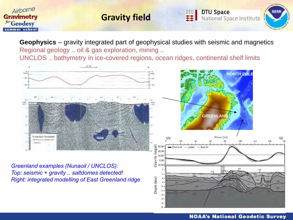
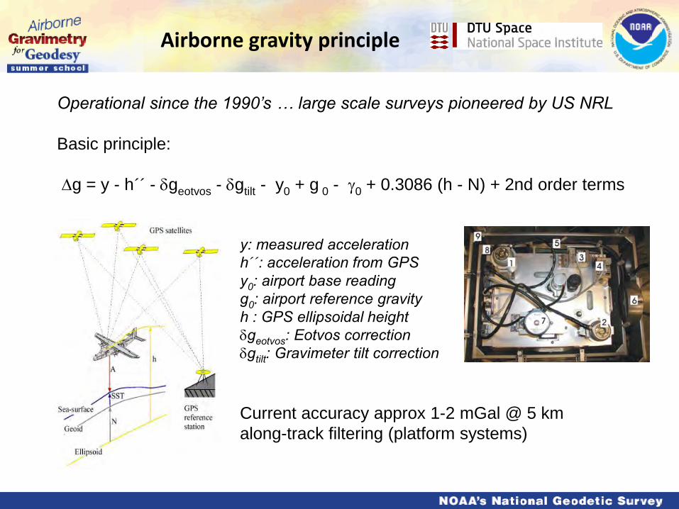
Operational since the 1990’s … large scale surveys pioneered by US NRL Basic principle: ∆g = y - h´´ - δgeotvos - δgtilt - y0 + g 0 - γ0 + 0.3086 (h - N) + 2nd order terms y: measured acceleration h´´: acceleration from GPS y0: airport base reading g0: airport reference gravity h : GPS ellipsoidal height δgeotvos: Eotvos correction δgtilt: Gravimeter tilt correction Current accuracy approx 1-2 mGal @ 5 km along-track filtering (platform systems)

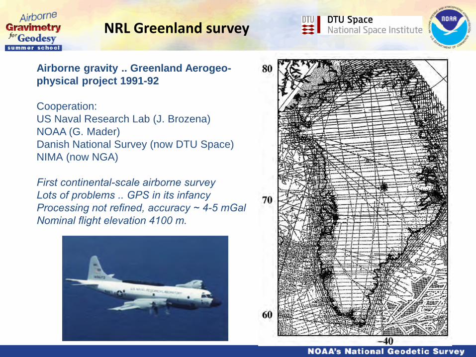
NRL Greenland survey

Airborne gravity .. Greenland Aerogeo- physical project 1991-92 Cooperation: US Naval Research Lab (J. Brozena) NOAA (G. Mader) Danish National Survey (now DTU Space) NIMA (now NGA) First continental-scale airborne survey Lots of problems .. GPS in its infancy Processing not refined, accuracy ~ 4-5 mGal Nominal flight elevation 4100 m.

Gravity – Arctic Ocean example

• Prime example of gravity signatures – submarine, surface, airborne data • Used for bathymetry inversion and sediment structures in UNCLOS projects (Denmark, Canada, US, Russia (VNIIOkeangeologia)

Arctic gravity project gravity compilation (DTU, SK, NGA, VNIIO, Tsniigaik, NRCan, ICESat, ...)

Airborne gravity surveys: 1992-2003 US NRL, DNSC-Norway, Canada, AWI Germany, Russia ..

US Naval Research Lab (Brozena)

ArcGP core data

Lomonosov Ridge airborne gravity and magnetic survey

DC3 used for airborne survey 2009 Russian icebreaker 50 Let Pobedy (LOMROG07 Denmark-Sweden-Russia)

• Airborne gravity and magnetics (LOMGRAV09 – DTU+NRCan) ~ 1.5 mGal r.m.s. error • Russian airborne surveys from Tiksi and Murmansk 2003-2006 • Icebreaker cruises with marine and helicopter gravimetry Grav + Mag -> structure and sediment thickness Fills GOCE polar gap Geoid useful for sea-ice altimetry

Arctic Ocean 2009 survey

Example: Malaysia 2002-3

Fig. 2a. Flight lines in East Malaysia. Colour coding represents flight elevation.

East Malaysia 2002 flight tracks First national large-scale survey dedicated for national geoid (GPS-RTK support) Carried out for JUPEM

West Malaysia flight tracks + existing data

Fig. 2b. Flight lines in East Malaysia. High elevation mainly due to airspace restrictions.

Fig. 3. Surface gravity coverage in East Malaysia (colours indicate anomalies)

Example: Malaysia 2002-3

Example: Malaysia 2002-3

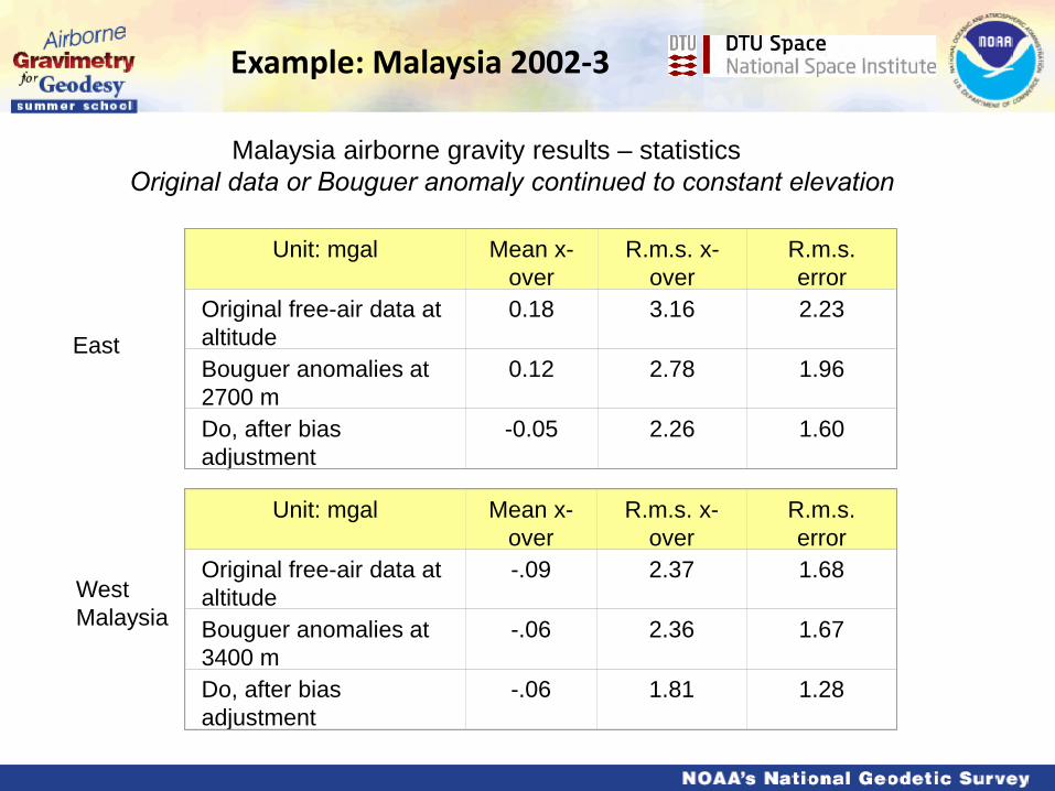
Malaysia airborne gravity results – statistics Original data or Bouguer anomaly continued to constant elevation

Unit: mgal

Mean x-over

R.m.s. x-over

R.m.s. error

Original free-air data at altitude

0.18

3.16

2.23

Bouguer anomalies at 2700 m

0.12

2.78

1.96

Do, after bias adjustment

-0.05

2.26

1.60

Unit: mgal

Mean x-over

R.m.s. x-over

R.m.s. error

Original free-air data at altitude

-.09

2.37

1.68

Bouguer anomalies at 3400 m

-.06

2.36

1.67

Do, after bias adjustment

-.06

1.81

1.28

East

West Malaysia

Malaysia airborne gravity results – Bouguer gravity maps

Example: Malaysia 2002-3

Final geoid models – revised 2008 due to Sumatra earthquake (fit in KL area after new re-levelling ~ 2 cm)

Example: Malaysia 2002-3

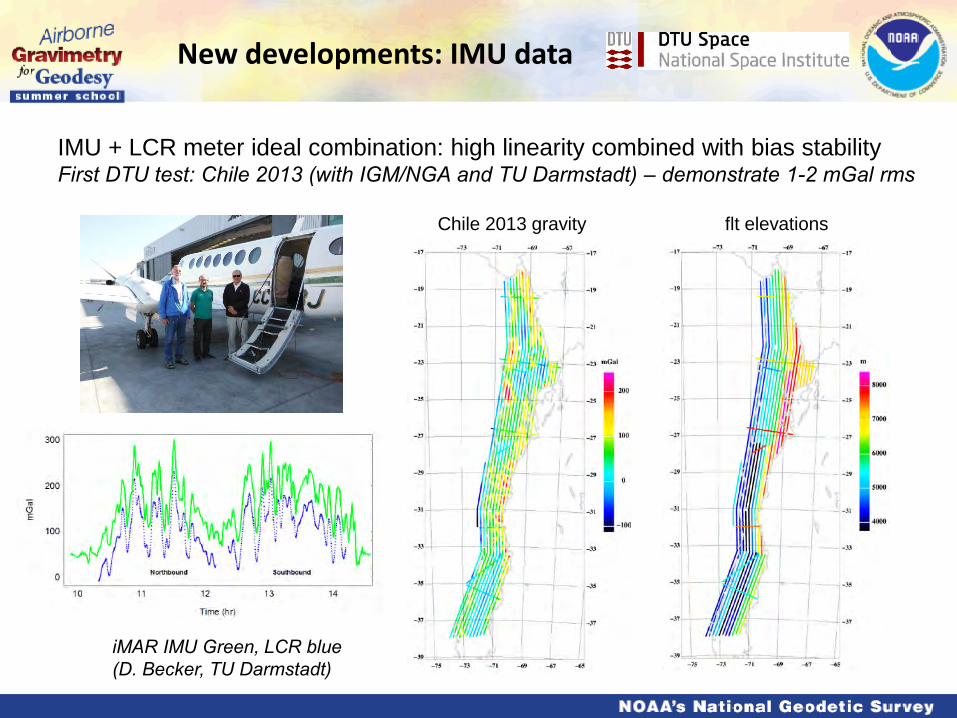
New developments: IMU data

IMU + LCR meter ideal combination: high linearity combined with bias stability First DTU test: Chile 2013 (with IGM/NGA and TU Darmstadt) – demonstrate 1-2 mGal rms

Chile 2013 gravity flt elevations

iMAR IMU Green, LCR blue (D. Becker, TU Darmstadt)

Satellite gravity: GOCE

Global gravity field from CHAMP, GRACE and GOCE … long-wavelength help aerogravity

Satellite gravity: GOCE

GOCE gradiometer GPS Tracking Drag-free satellite measurements Orbit inclination 83° => Polar gap!

Global geoid models available as spherical harmonics data to degree 260 from European GOCE Consortium Latest model R5 Complete GOCE Mission data GOCE dived into low

Earth orbit in final months (240 -> 230 -> 225 km)

Satellite gravity: GOCE

2160

Airborne gravity

GOCE observations: Gravity gradients … (SGG: Tzz, Txx etc) GOCE Level-2 data in spherical harmonics:

[ ] )(sinPsincos)(),,( ϕλλλφ nmnmnm

n

=0m2=n

m D + m Cn

Rr

rGM = rT −∑∑

∞

GRACE limitation ~ degree 90 GOCE to degree ~ 220-240 Airborne ~ degree 2160 (5’) Surface data ~ degree 10000 (1’)

Gravity validation: GOCE

SE-Asia Comparison to GOCE

as a function of max degree N (R5 direct)

Unit: mGal

N Mean Stddev

Data 45.3 31.2

180 1.1 39.7

200 0.6 36.9

220 0.2 34.3

240 0.0 32.6

260 -0.1 30.7

280 -0.0 30.7 DTU Surveys - r.m.s. error 1.8-2.5 mGal

Philippines 2012-13

Malaysia 2002-3

Indonesia 2008-11

Gravity validation: GOCE

-21

-19

-17

-15

0 300 600 900 1200 1500 1800 2100

Degree

Log

[deg

ree

varia

nce]

Surface data

GOCE data

Surface – GOCE data GOCE

Zoom-In

Spectral analysis for GOCE validation Malaysia/Indonesia/Phillipines DTU surveys Method: - Fill-in by EGM08 (mainly marine) - 2D PSD estimation with FFT - Isotropic averaging of PSD - Conversion to degree variance σ

Surface – GOCE

Back to theory ..

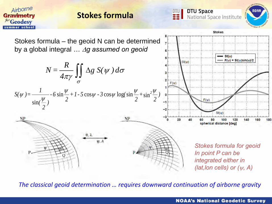
Stokes formula

σψπγ

σ

d ) S(g 4

R = N ∫∫ ∆

)2

+2

( 3 - 5 - 1 + 2

6 - )

2(

1 = )S( 2ψψψψψψ

ψ sinsinlogcoscossinsin

Stokes formula – the geoid N can be determined by a global integral … ∆g assumed on geoid

Stokes formula for geoid In point P can be integrated either in (lat,lon cells) or (ψ, A)

The classical geoid determination … requires downward continuation of airborne gravity

σψπγ

ζσ

d ) S()g+g( 4

R = 1∆∫∫

Non-level surface => Molodenskys formula: ζ is quasi-geoid

Definition of gravity anomaly: Refers to surface of topography!

H h

+ -g -g = g oobservedPP

observedPP ∂

∂≈∆ ′

γγγ

Geoid and quasigeoid

Remove-restore methods

General remove-restore terrain reductions

“Remove” “Restore” Case of geoid computation from gravity Gravity and geoid functionals Case of downward/upward continuation Make RTM- or Bouguer anomalies -> downward continue -> restore terrain

( ) ( ) ( )mobsobscobs TLTLTL −=

( ) ( ) ( )mpredc

predpred TLTLTL +=

predobs LL →

( ) ( ) Trr

TTLTL gobs2

−∂∂

−−= ∆

( ) ( )γζTTLTLpred ==

Remove long wavelengths: EGM2008/GOCE combination Remove shorter wavelengths: terrain effects (e.g. from SRTM)

Terrain effect types

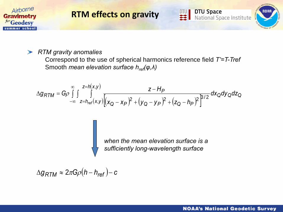
RTM gravity anomalies Correspond to the use of spherical harmonics reference field T’=T-Tref Smooth mean elevation surface href(φ,λ)

( ) ( ) ( )[ ]( )

( )∫ ∫ ∫∞

∞−

=

= −+−+−

−=∆

yxhz

yxhzQQQ

PQPQPQ

PRTM

ref

dzdydxhzyyxx

HzGg,

,2/3222

ρ

( ) chhGg refRTM −−≈∆ ρπ2

when the mean elevation surface is a sufficiently long-wavelength surface

RTM effects on gravity

Terrain effects: prisms

• The rectangular prism of constant density is a useful "building block" for numerical integrations of the basic effects – gravity and geoid formulas:

z+y+x =r

,|||zrxyz -r)+(xy + r)+(y x|||G = g

222

zz

yy

xxm

12

12

12

arctanloglogρδ

||| zrxy

2z -

yrxz

2y -

xryz

2x -

r)+(xyz +r)+(yxz + r)+(zxy |||G = T

zz

yy

xx

222

m

12

12

12

arctanarctanarctan

logloglogρ

• Bouguer anomalies .. require DEM and terrain corrections .. 3’ SRTM data perfect data source.

Prism approximations

Approximation in spherical harmonics (larger distances)

Efficient implementations (GRAVSOFT TC):

• Coarse/detailed grid

• Splines in inner zone

• Use of station heights (inner zone modification)

( ) ( )[

( ) ] [ ]

+++∆+∆−∆−+

∆−∆+∆−+∆−∆−∆+∆∆∆=

449

2222

222222225

28812

2224

11

yxr

zzyx

yzyxxzyxrr

zyxGTm

βα

ρ

121212 ,, zzzyyyxxx −=∆−=∆−=∆

• Basic definition of 2-D Fourier transform

• kx and ky are called wavenumbers (like frequency in 1-D time domain) … defined on infinite x-y plane

yxykxki

yx

ykxkiyx

dkdkekkGyxgGF

dxdyeyxgkkFgF

yx

yx

∫∫∫∫

+−

+−

==

==

)(2

1

)(

),(4

1),()(

),(),()(

π

Advantage of Fourier transforms: convolution theorem

• Convolutions must faster in frequency domain than space domain …many geodetic integrals can be expressed as convolutions

)()()*(

'')','()','(),(*

gFfFgfF

dydxyxgyyxxfyxgf

⋅=⇒

−−= ∫∫

g F(g)

2-D Fourier transforms

• Derivates of Fourier transform:

• Vertical derivates from upward continuation formula:

• Anomalous potential relationships follows from these (allow the direct determination of geoid: transform + filter + inverse transform!)

)()(

)()()()/2()(

TFkF

TFkFTFrkgF

x

y

γη

γξ

−=

−=+=∆

)()( gFikxgF x δ=∂∂

22

))0,,(()),,((

yx

kz

kkk

eyxgFzyxgF

+=

= −δδ

FFT and gravity field quantities

Basic equations for geoid determination, deflections, upw.continuation – in planar approximation (on sphere: spherical FFT ….)

The terrain correction as convolutions

[ ]dxdy

syxhyxhGyxc

E

PPPP ∫∫

−= 3

0

2),(),(21),( ρ ),(),(),,(),(,

21 3

02 yxsyxryxhyxnGK −=== ρ

( ) ( ) ( )[ ]PpPpPpPP yxtyxtyxtKyxc ,,,),( 321 ++=

( ) ∫∫ −−=E

PPPP dxdyyyxxryxnyxt ),(),(,1

( ) ( )∫∫ −−−=E

PPPPPP dxdyyyxxryxhyxhyxt ),(),(,2,2

( ) ∫∫ −−=E

PPPPPP dxdyyyxxryxnyxt ),(),(,3

( ) ( )[ ])0,0(2 22 RhrhhrhKc PPP +∗−∗=Final formula – c as convolutions in h and h2: Convolutions very fast evalutated by FFT: Much more in IAG geoid schools …

Terrain corrections by FFT

Airborne terrain effects by FFT

( ) ( ) ( ) ( )[ ]yxkyxhyxkyxhGzGzyxc avPP ,,,,2),,( 22110 ∗+∗+−= ρρπ

• Integration with respect to z

• Applying some analytical evaluations

• Introducing into the derivations Zav (mean height of elevations)

avzyxhyxh −= ),(),(1

[ ]22 ),(),( avzyxhyxh −=

( ) ( )( )[ ] 2/32

022

01 ,

av

av

zzyx

zzyxk

−++

−−= ( )

( )[ ]( )

( )[ ] 2/320

22

02/32

022

22

3

2

1,av

av

av zzyx

zz

zzyxyxk

−++

−−

−++=

Analytical derivation in Tziavos et al. (1988)

Downward continuation

Downward continuation of airborne gravity important application of spatial least-squares collocation (planar or spherical self-consistent models)

s is ”signal” (prediction quantity), x ”observation”, Csx = cov(Ls(T), Lx(T)) from model

- The covariance model must be harmonic: ∆ {cov( · ,T)} = 0

- Use of remove-restore terrain reductions stabilizes solution

- May be done blockwise .. e.g. 1º x 1 º blocks with overlap … makes solution fast, avoiding very large sets of linear equations

Alternative for constant-elevation surveys: Fourier transformation

F [∆g(x,y,h)] = e-kh F [∆g(x,y,0)]

k = √(kx2+ky

2)

1][ −+= DCCs xxsx

Downward continuation (2)

Self-consistent covariance model for aerogravity

iTDD

hhDsDCggC

i

iiii

hh

−=

++++−=∆∆ ∑=

4

1

221

20 )(log(),( 21 α

• Planar domain ok for downward continuation of airborne data • Requirement: spatial analytical covariance function model - e.g. Tscherning-Rapp model on sphere - globall - e.g. planar logaritmic model - planar

Model fitted to empirical data by three parameters: C0, D, T - D corresponding to Bjerhammar sphere depth - T is a long-wavelength attenuation ”compensation depth” - Complete formulas for gravity, geoid, 2nd order gradients in Forsberg (1987) … useful for downward continuation, deflections and gradiometry

Spherical Tscherning-Rapp model

Deflections of the vertical

Vector gravimetry – PEI, Canada (S. Ferguson/SGL & Forsberg, AGU 2012)

Data: SRTM DEM (Quite benign region) NRCan /GSDgravimetry (M. Veronneau)

Vector gravimetry data – SGL survey

SGL AIRGRAV survey tied to g-value at airport; converted to gravity anomaly using EGM08 geoid. Deflections of the vertical fitted by survey-wide bias and slope to EGM08. Comparison SGL ∆g minus GSD ∆g: mean = 0.3 mgal, r.m.s. 1.5 mgal (points within 500 m; no downward continuation) => excellent quality!

Flight elevation ~ 1000 ft

PEI geoid comparison

Geoid predictions by FFT compared to GSD GPS-levelling on PEI (18 1st order points) Blue rows: What would happen if only GOCE and SGL data available?

GPS levelling – geoid from NRCan gravity Comparison of geoid solutions

Geoid model

Mean (m)

Std.dev. (m)

Geoid from NRCan data only + RTM

-0.056 0.031

Geoid from SGL gravity + RTM -0.069 0.032

CGG10 NRCan geoid model -0.013 0.039

Geoid from GOCE only -0.122 0.262

Geoid from GOCE and SGL gravity -0.124 0.216

DoV comparison

Line 25 – E-W line through center of island (deflections fitted by bias and slope). Black: observed data; green: ”Best” FFT solution; pink: CGG10 deflections Results show horizontal gravity accurate @ 1-2 mgal accuracy (1” ~ 4.8 mGal)

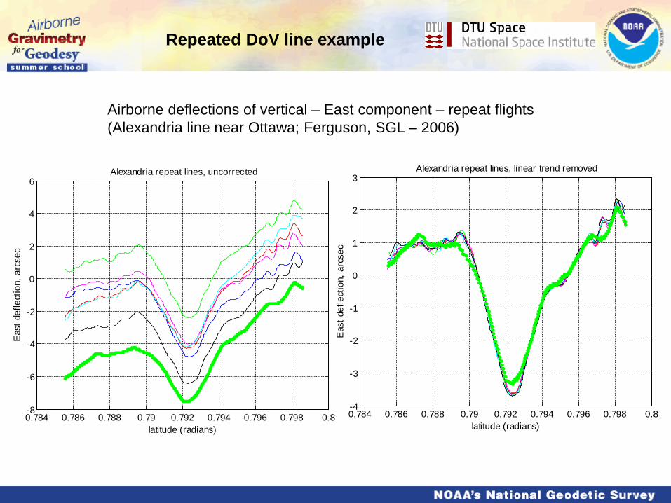
Repeated DoV line example

Airborne deflections of vertical – East component – repeat flights (Alexandria line near Ottawa; Ferguson, SGL – 2006)

0.784 0.786 0.788 0.79 0.792 0.794 0.796 0.798 0.8-8

-6

-4

-2

0

2

4

6Alexandria repeat lines, uncorrected

latitude (radians)

Eas

t def

lect

ion,

arc

sec

0.784 0.786 0.788 0.79 0.792 0.794 0.796 0.798 0.8-4

-3

-2

-1

0

1

2

3Alexandria repeat lines, linear trend removed

latitude (radians)

Eas

t def

lect

ion,

arc

sec

Summary

• Airborne gravity complements surface and satellite gravity … GOCE R5 models agree with airborne data to degree 200-220 (except polar gaps >83°)

• Important to understand processing parameters for merging data from separate surveys (e.g., disturbance or free-air anomalies, atmospheric corrections applied, filtering parameters etc.)

• Gravity field modelling in 3D allows optimal combination of all available data - least-squares collocation combined by Fourier methods efficient

• Terrain effects important – Bouguer anomaly computations for geophysics, stabilization of downward continuation for merged free-air anomaly grid for geoid determination or prediction of deflections of the vertical

• Deflections of the vertical can be handled analogous to (vertical) gravity – full vector gravimetry systems operational ..

More on geoid determination and GRAVSOFT in Wednesday talk/demo