The Value of Energy Storage and Demand Response for ... describing energy storage and demand...
241
Energy Research and Development Division FINAL PROJECT REPORT THE VALUE OF ENERGY STORAGE AND DEMAND RESPONSE FOR RENEWABLE INTEGRATION IN CALIFORNIA FEBRUARY 2017 CEC-500-2017-014 Prepared for: California Energy Commission Prepared by: Lawrence Livermore National Laboratory
Transcript of The Value of Energy Storage and Demand Response for ... describing energy storage and demand...

E n e r g y R e s e a r c h a n d D e v e l o p m e n t D i v i s i o n F I N A L P R O J E C T R E P O R T
THE VALUE OF ENERGY STORAGE AND DEMAND RESPONSE FOR RENEWABLE INTEGRATION IN CALIFORNIA
FEBRUARY 2017 CE C-500-2017-014
Prepared for: California Energy Commission Prepared by: Lawrence Livermore National Laboratory

PREPARED BY: Primary Author(s): Thomas Edmunds Alan Lamont Vera Bulaevskaya Carol Meyers Jeffrey Mirocha Andrea Schmidt Matthew Simpson Steven Smith Pedro Sotorrio Philip Top Yiming Yao Lawrence Livermore National Laboratory 7000 East Avenue Livermore CA 94550 925-422-1100 www.llnl.gov Contract Number: 500-10-051 Prepared for: California Energy Commission Avtar Bining, Ph.D. Contract Manager Fernando Piña Office Manager Energy Systems Research Office Laurie ten Hope Deputy Director ENERGY RESEARCH AND DEVELOPMENT DIVISION Robert P. Oglesby Executive Director
DISCLAIMER This report was prepared as the result of work sponsored by the California Energy Commission. It does not necessarily represent the views of the Energy Commission, its employees or the State of California. The Energy Commission, the State of California, its employees, contractors and subcontractors make no warranty, express or implied, and assume no legal liability for the information in this report; nor does any party represent that the uses of this information will not infringe upon privately owned rights. This report has not been approved or disapproved by the California Energy Commission nor has the California Energy Commission passed upon the accuracy or adequacy of the information in this report.

i
ACKNOWLEDGEMENTS
The authors would like to thank Michael Gravely, Avtar Bining, Steve Ghadiri, and Ivin Rhyne at the California Energy Commission for their support and guidance. The authors would also like to thank the following persons for their advice, data resources, references to other works, and software support:
Mark Rothleder, Clyde Loutan, Shucheng Liu, Edward Lo, James Price, and John Goodman, California Independent System Operator
Glenn Drayton, Julian Hamilton, and David Llewellyn, Energy Exemplar, LLC
Wenxiong Huang, Plexos Solutions, LLC
Warren Katzenstein and Ralph Masiello, DNV GL Group
Guojing Cong, IBM Corp.
Sila Kiliccote, Mary Anne Piette, and Nance Matson, Demand Response Research Center
Benjamin Kaun, Haresh Kamath, and Robert Schainker, Electric Power Research Institute
Giovanni Damato, Strategen Corp. representing California Energy Storage Alliance
Chi-Fan Shih and Karen Gibson, National Center for Atmospheric Research
Alexandra von Meier, California Institute for Energy and Environment
Ronald Hofmann, Consultant
Antonio Alvarez, Alva Svoboda, and Daidipya Patwa, Pacific Gas and Electric Company
Udi Helman, consultant
Other technical peer reviewers

ii
PREFACE
The California Energy Commission Energy Research and Development Division supports public interest energy research and development that will help improve the quality of life in California by bringing environmentally safe, affordable, and reliable energy services and products to the marketplace.
The Energy Research and Development Division conducts public interest research, development, and demonstration (RD&D) projects to benefit California.
The Energy Research and Development Division strives to conduct the most promising public interest energy research by partnering with RD&D entities, including individuals, businesses, utilities, and public or private research institutions.
Energy Research and Development Division funding efforts are focused on the following RD&D program areas:
• Buildings End-Use Energy Efficiency
• Energy Innovations Small Grants
• Energy-Related Environmental Research
• Energy Systems Integration
• Environmentally Preferred Advanced Generation
• Industrial/Agricultural/Water End-Use Energy Efficiency
• Renewable Energy Technologies
• Transportation
The Value of Energy Storage and Demand Response for Renewable Integration in California is the final report for the Planning for Generation, Storage, and Demand Response to Accommodate Intermittent Generation project (Contract Number 500-10-051 conducted by Lawrence Livermore National Laboratory. The information from this project contributes to Energy Research and Development Division’s Energy Systems Integration Program.
When the source of a table, figure or photo is not otherwise credited, it is the work of the author of the report.
For more information about the Energy Research and Development Division, please visit the Energy Commission’s website at www.energy.ca.gov/research/ or contact the Energy Commission at 916-327-1551.

iii
ABSTRACT
Increased contributions from wind and solar power resources are necessary to meet California’s goal to use 33 percent renewable energy by 2020. Using these renewable resources, however, will substantially increase the variability and uncertainty in electricity generation resources available to California’s electricity grid operators. Automated demand response and energy storage systems can help reduce this variability and uncertainty through energy buying and selling (arbitrage) in day-ahead markets that would levelize loads and prices throughout the day. They could also provide load-following capability through bids in the real-time market and system management (or regulation) services to the system operator. The project identified policies, technologies (energy storage), and control methods (demand response) that could reduce the cost and improve the reliability of electric power for California ratepayers. Data and assumptions describing energy storage and demand response resources were provided by the Electric Power Research Institute, the California Energy Storage Alliance, and the Demand Response Research Center. The California Independent System Operator provided the production simulation model and supporting data.
Keywords: Demand response, storage, load following, regulation, renewable generation, weather forecast, production simulation, unit commitment
Please use the following citation for this report:
Edmunds, Thomas, Alan Lamont, Vera Bulaevskaya, Carol Meyers, Jeffrey Mirocha, Andrea Schmidt, Matthew Simpson, Steven Smith, Pedro Sotorrio, Philip Top, and Yiming Yao Lawrence Livermore National Laboratory. 2017. The Value of Energy Storage and Demand Response for Renewable Integration in California. California Energy Commission. Publication number: CEC-500-2017-014.

iv
TABLE OF CONTENTS
Acknowledgements .................................................................................................................................. 1
PREFACE .................................................................................................................................................... 2
ABSTRACT ................................................................................................................................................ 3
TABLE OF CONTENTS ........................................................................................................................... 4
LIST OF FIGURES .................................................................................................................................... 8
LIST OF TABLES .................................................................................................................................... 13
EXECUTIVE SUMMARY ........................................................................................................................ 1
Introduction ........................................................................................................................................ 1
Project Purpose ................................................................................................................................... 1
Project Process .................................................................................................................................... 1
Project Results ..................................................................................................................................... 2
Project Benefits ................................................................................................................................... 4
CHAPTER 1: Introduction ....................................................................................................................... 5
1.1 Strategies for Meeting California’s Renewable Portfolio Standard .................................... 5
1.2 Overall Analysis Approach ...................................................................................................... 6
1.3 Previous Work ............................................................................................................................ 7
1.4 Scope of This Report .................................................................................................................. 9
CHAPTER 2: Atmospheric Modeling Method .................................................................................. 10
2.1 Weather Model Description.................................................................................................... 11
2.2 Model Domain Configuration ................................................................................................ 11
2.3 Ensemble Atmospheric Forecasts .......................................................................................... 13
2.3.1 Ensemble Configuration ................................................................................................. 15
2.3.2 Input Data ......................................................................................................................... 16
2.3.3 Four-Dimensional Data Assimilation............................................................................ 17
2.4 Synthetic Weather Observations ............................................................................................ 18
2.5 Computation Time and Storage Demands ........................................................................... 19
2.6 Weather Model Validation ..................................................................................................... 19

v
2.7 Example Ensemble Forecasts and LIDAR Measurements ................................................. 30
CHAPTER 3: Wind and Solar Power From WRF Output ................................................................ 32
3.1 Determination of Sites to Be Used for Wind and Solar ...................................................... 33
3.2 Technology and Geometry Assumptions for Solar PV ....................................................... 33
3.3 WRF Domains ........................................................................................................................... 34
3.4 Calculation of Solar Power From Downward Radiative Flux ........................................... 36
3.5 Placement of Wind Farms Within Grid Cells ....................................................................... 41
3.6 Calculation of Wind Power From Wind Speed ................................................................... 45
3.7 Aggregation of Wind and Solar Sites Into PLEXOS Model Regions ................................ 46
4.1 Load Adjustments for Temperature ...................................................................................... 49
4.1.1 Generation of Load Adjustment Equations .................................................................. 50
4.1.2 Calculation of ΔL/ΔT ....................................................................................................... 50
4.1.3 Calculation of a Load-Weighted Temperature for Each California Region............. 54
4.1.4 Calculation of Load Changes for Each Trajectory ....................................................... 55
4.1.5 PLEXOS Load Profiles by Region .................................................................................. 55
4.2 Example Net Load Data .......................................................................................................... 56
CHAPTER 5: Clustering and Selection of Trajectories .................................................................... 58
5.1 Key Features of Net Load Trajectories .................................................................................. 59
5.2 Trajectory Reduction Results .................................................................................................. 60
5.3 Approaches Used by Other Researchers .............................................................................. 63
CHAPTER 6: Production Simulation Modeling ............................................................................... 64
6.1 Analysis Process ....................................................................................................................... 64
6.1.1 Storage and Demand Response Capacities .................................................................. 65
6.2 Production Simulation Modeling With PLEXOS Software ................................................ 66
6.2.1 Stochastic Unit Commitment.......................................................................................... 67
6.2.2 Interleaved Timescales .................................................................................................... 67
6.3 Regulation and System Stability Modeling .......................................................................... 68
6.3.1 Regulation Analysis ......................................................................................................... 69

vi
6.3.2 Stability Analysis .............................................................................................................. 69
CHAPTER 7: Extensions to California ISO High Load Model ...................................................... 71
7.1 Description of the WECC Regional Model ........................................................................... 71
7.2 Modeling Demand Response ................................................................................................. 73
7.2.1 Characterization of Demand Response Resources ...................................................... 73
7.2.2 Modeling Demand Response in PLEXOS ..................................................................... 75
7.3 Modeling Storage ..................................................................................................................... 76
7.4 Cases for Analysis .................................................................................................................... 77
CHAPTER 8: Results From Production Simulation Model ............................................................ 79
8.1 Commitment and Economic Dispatch Patterns ................................................................... 79
8.1.1 Original Case Dispatch .................................................................................................... 79
8.1.2 Baseline Case Dispatch .................................................................................................... 82
8.2 Prices .......................................................................................................................................... 83
8.2.1 Original Case Prices and Revenues ............................................................................... 83
8.2.2 Baseline Case Prices and Revenues ............................................................................. 106
8.3 Clustering Days ...................................................................................................................... 111
CHAPTER 9: Value of DR and Storage for Regulation ................................................................. 115
9.1 Cost Reductions From DR for Regulation .......................................................................... 115
9.1.1 Total Cost Reductions With DR ................................................................................... 115
9.1.2 Sources of Costs Savings With DR .............................................................................. 116
9.2 Cost Reductions of Storage for Regulation ......................................................................... 118
CHAPTER 10: Demand Response and Storage for Load Following and Energy Arbitrage ... 121
10.1 Load Following Requirements ............................................................................................. 121
10.2 Scenarios for Analysis of DR ................................................................................................ 121
10.3 Scenarios for Analysis of Storage ......................................................................................... 123
10.3.1 Operation of Energy Storage ........................................................................................ 123
10.3.2 Total Net Revenue and Marginal Value of Storage................................................... 124
10.4 Results for Energy Storage for Load Following and Energy Arbitrage ......................... 125

vii
10.4.1 Cases Analyzed .............................................................................................................. 125
10.4.2 Economic Dispatch of Storage Operations ................................................................. 126
10.4.3 Value of Storage ............................................................................................................. 130
10.5 Revenues From Ancillary Services ...................................................................................... 137
10.6 Investment Analysis of Storage Capacity ........................................................................... 140
CHAPTER 11: Regulation and Stability Assessment ..................................................................... 142
11.1 Regulation Assessment ......................................................................................................... 142
11.1.1 Model Development ...................................................................................................... 142
11.1.2 Metrics ............................................................................................................................. 144
11.1.3 Analysis Procedure ........................................................................................................ 144
11.1.4 Regulation Errors ........................................................................................................... 146
11.1.5 Regulation Analysis Results ......................................................................................... 147
11.1.6 Energy Limitations of Batteries Providing Regulation ............................................. 152
11.2 Stability Assessment .............................................................................................................. 154
11.2.1 Factors Affecting Stability ............................................................................................. 154
11.2.2 Stability Analysis Procedure ........................................................................................ 155
11.2.3 Stability Analysis Results .............................................................................................. 158
11.2.4 Contingency Event Magnitude Tests .......................................................................... 165
11.2.5 Stability Assessment ...................................................................................................... 166
CHAPTER 12: Summary and Conclusions ....................................................................................... 167
12.1 Modeling and Data ................................................................................................................ 167
12.2 Value of Demand Response and Storage ............................................................................ 168
12.3 Regulation and Stability ........................................................................................................ 169
GLOSSARY ............................................................................................................................................ 171
REFERENCES ........................................................................................................................................ 173
APPENDIX A: Solar and Wind Sites Used in Weather Model .................................................... A-1
APPENDIX B: Example Net Load Trajectories ................................................................................ B-1
APPENDIX C: Demand Response Programs and Data ................................................................. C-1

viii
APPENDIX D: Storage Data ............................................................................................................... D-1
APPENDIX E: Case Descriptions ....................................................................................................... E-1
APPENDIX F: Stakeholder Relevance .............................................................................................. F-1
APPENDIX G: Peer Review Summary............................................................................................. G-1
LIST OF FIGURES Figure ES-1: Annual Net Revenues for Energy Storage (4-Hour Discharge) .................................... 2
Figure ES-2: Annual Net Revenues for 50 Megawatts of Storage for Each Technology .................. 3
Figure 1-1: Renewable Generation, Production Simulation, and Resource Evaluation Process .... 6
Figure 2-1: Atmospheric Model Domain Configuration .................................................................... 12
Figure 2-2: Location of Wind and Solar Resources Within Model Domains ................................... 13
Figure 2-3: Illustration of WRF Multiphysics Ensemble Wind Speed Forecast .............................. 15
Figure 2-4: Temperature Forecasts and Measurements – Bakersfield, April 1................................ 21
Figure 2-5: Temperature Forecasts and Measurements – Bakersfield, April 15.............................. 21
Figure 2-6: Temperature Forecasts and Measurements – Bakersfield, August 1 ............................ 22
Figure 2-7: Temperature Forecasts and Measurements – Bakersfield, August 15 .......................... 22
Figure 2-8: Temperature Forecasts and Measurements – Bakersfield, Nov. 1 ................................ 23
Figure 2-9: Temperature Forecasts and Measurements – Bakersfield, Nov. 15 .............................. 23
Figure 2-10: Temperature Forecasts and Measurements – Ontario, April 15 .................................. 24
Figure 2-11: Temperature Forecasts and Measurements – Ontario, August 15 .............................. 24
Figure 2-12: Temperature Forecasts and Measurements – Ontario, Nov. 15 .................................. 25
Figure 2-13: Wind Speed Forecasts and Measurements – Bakersfield, April 1 ............................... 25
Figure 2-14: Wind Speed Forecasts and Measurements – Bakersfield, April 15 ............................. 26
Figure 2-15: Wind Speed Forecasts and Measurements – Bakersfield, August 1 ........................... 26
Figure 2-16: Wind Speed Forecasts and Measurements – Bakersfield, August 15 ......................... 27
Figure 2-17: Wind Speed Forecasts and Measurements – Bakersfield, Nov. 1 ............................... 27
Figure 2-18: Wind Speed Forecasts and Measurements – Bakersfield, Nov. 15 ............................. 28
Figure 2-19: Wind Speed Forecasts and Measurements – Ontario, April 15 ................................... 28
Figure 2-20: Wind Speed Forecasts and Measurements – Ontario, August 15 ............................... 29
ix
Figure 2-21: Wind Speed Forecasts and Measurements – Ontario, Nov. 15 .................................... 29
Figure 2-22: WRF Multiphysics Ensemble Wind Speed Forecast and LIDAR Measurements ..... 30
Figure 2-23: WRF Multianalysis and Multiphysics Forecasts With LIDAR Measurements ......... 31
Figure 3-1: WRF Atmospheric Model Domains and Renewable Energy Production Plants ........ 35
Figure 3-2: Path of Sun in Celestial Sphere ........................................................................................... 37
Figure 3-3: Schematic of Unit Vector Describing Sun Location ......................................................... 38
Figure 3-4: Schematic of Unit Vector Describing Solar Panel Orientation ....................................... 39
Figure 3-5: Ensemble Solar Flux and Power Prediction at One Solar Power Plant ........................ 41
Figure 3-6: Modeled Wind Power Plants Near Tehachapi, California ............................................. 42
Figure 3-7: Power Curve for Vestas V90 Wind Turbine ..................................................................... 45
Figure 3-8: Ensemble Wind Speed and Power Prediction at One Wind Power Plant ................... 46
Figure 3-9: Map of All Wind and Solar Projects .................................................................................. 47
Figure 4-1: Load Versus Temperature for California ISO .................................................................. 51
Figure 4-2: Second Order Polynomial Fit for Single Hour and Weekday ........................................ 52
Figure 4-3: Standard Deviation of Prediction Error ............................................................................ 52
Figure 4-4: Fit of ΔLoad/ΔTemp Data ................................................................................................... 53
Figure 4-5: ΔL/ΔT Versus Temperature and Hour of the Day .......................................................... 54
Figure 4-6: Ensemble of Net Loads in California for the Week of April 5-11, 2020 ........................ 56
Figure 4-7: Ensemble of Net Loads in California for April 9, 2020 ................................................... 57
Figure 5-1: Computation Time Versus Number of Net Load Trajectories ...................................... 58
Figure 5-2: Clustering of April 9, 2020, Trajectories ............................................................................ 60
Figure 5-3: Trajectories Selected to Represent the 30-Member Ensemble for April 9, 2020 .......... 62
Figure 6-1: Analysis Process ................................................................................................................... 64
Figure 6-2: Marginal Value of Storage .................................................................................................. 66
Figure 6-3: Time Horizons of the PLEXOS Model ............................................................................... 68
Figure 6-4: System Stability Analysis .................................................................................................... 70
Figure 7-1: Demand Response Availability by Source and Total in SCE on August 2, 2020 ........ 75
Figure 8-1: Generation Pattern for January 15 (Original Case) ......................................................... 79

x
Figure 8-2: Generation Pattern for April 28 (Original Case) .............................................................. 80
Figure 8-3: Generation Pattern for June 24 (Original Case) ............................................................... 80
Figure 8-4: Generation Pattern for August 13 (Original Case) .......................................................... 81
Figure 8-5: Generation Pattern for November 12 (Original Case) .................................................... 81
Figure 8-6: Generation Pattern for January 15 (Baseline Case) .......................................................... 83
Figure 8-7: Generation Pattern for August 13 (Baseline Case) .......................................................... 83
Figure 8-8: Energy Prices for January 15 (Original Case) ................................................................... 84
Figure 8-9: Ancillary Services Prices January 15 (Original Case) ...................................................... 85
Figure 8-10: Load Following Capacities Required on January 15 (Original Case) ......................... 86
Figure 8-11: Load Following Prices January 15 (Original Case) ........................................................ 87
Figure 8-12: California Total Hourly Costs on January 15 (Original Case) ..................................... 87
Figure 8-13: WECC Hourly Total Cost on January 15 (Original Case) ............................................. 88
Figure 8-14: Energy Prices for April 28 (Original Case) ..................................................................... 89
Figure 8-15: Ancillary Services Prices April 28 (Original Case) ........................................................ 89
Figure 8-16: Load Following Capacities Required on April 28 (Original Case) .............................. 90
Figure 8-17: Load Following Prices April 28 (Original Case) ............................................................ 90
Figure 8-18: California Total Hourly Costs on April 28 (Original Case) .......................................... 91
Figure 8-19: WECC Hourly Total Cost on April 28 (Original Case) ................................................. 92
Figure 8-20: Energy Prices for June 24 (Original Case) ....................................................................... 92
Figure 8-21: Ancillary Services Prices June 24 (Original Case) .......................................................... 93
Figure 8-22: Load Following Requirements on June 24 (Original Case) .......................................... 94
Figure 8-23: Load Following Prices June 24 (Original Case) ............................................................. 94
Figure 8-24: California Total Hourly Costs on June 24 (Original Case) ........................................... 95
Figure 8-25: WECC Hourly Total Cost on June 24 (Original Case) .................................................. 95
Figure 8-26: Energy Prices for August 13 (Original Case).................................................................. 96
Figure 8-27: Ancillary Services Prices August 13 (Original Case) .................................................... 96
Figure 8-28: Load Following Requirements for August 13 (Original Case) .................................... 97
Figure 8-29: Load Following Prices August 13 (Original Case) ........................................................ 97

xi
Figure 8-30: California Total Hourly Costs on August 13 (Original Case) ...................................... 98
Figure 8-31: WECC Hourly Total Costs on August 13 (Original Case) ............................................ 98
Figure 8-32: Energy Prices for November 12 (Original Case) ............................................................ 99
Figure 8-33: Ancillary Services Prices November 12 (Original Case) ............................................... 99
Figure 8-34: Load Following Requirements on November 12 (Original Case) ............................. 100
Figure 8-35: Load Following Prices November 12 (Original Case) ................................................. 100
Figure 8-36: California Total Hourly Costs on November 12 (Original Case) .............................. 101
Figure 8-37: WECC Hourly Total Costs on November 12 (Original Case) .................................... 102
Figure 8-38: Energy Prices by Day and Hour of the Year (Original Case) ..................................... 102
Figure 8-39: Load Following Up Prices by Day and Hour of the Year (Original Case) ............... 103
Figure 8-40: Load Following Down Prices by Day and Hour of the Year (Original Case) ......... 103
Figure 8-41: Regulation Up Prices by Day and Hour of the Year (Original Case) ....................... 104
Figure 8-42: Regulation Down Prices by Day and Hour of the Year (Original Case) .................. 104
Figure 8-43: Spinning Reserve Prices by Day and Hour of the Year (Original Case) .................. 105
Figure 8-44: Nonspinning Reserve Prices by Day and Hour of the Year (Original Case) ........... 105
Figure 8-45: Annual Revenues from Energy and Ancillary Services (Original Case) .................. 106
Figure 8-46: Energy Prices for January 15 (Baseline Case) ............................................................... 106
Figure 8-47: Ancillary Services Prices January 15 (Baseline Case) .................................................. 107
Figure 8-48: Load Following Prices January 15 (Baseline Case) ...................................................... 107
Figure 8-49: California Total Hourly Costs on January 15 (Baseline Case) ................................... 108
Figure 8-50: WECC Hourly Total Costs on January 15 (Baseline Case) ......................................... 108
Figure 8-51: Energy Prices for June 24 (Baseline Case) ..................................................................... 109
Figure 8-52: Ancillary Services Prices June 24 (Baseline Case) ........................................................ 109
Figure 8-53: Load Following Prices June 24 (Baseline Case) ............................................................ 110
Figure 8-54: California Total Hourly Costs on June 24 (Baseline Case) ......................................... 110
Figure 8-55: WECC Hourly Total Costs on June 24 (Baseline Case) ............................................... 111
Figure 8-56: One Day Representing a Cluster .................................................................................... 112
Figure 8-57: Comparison of Prices on Cluster Days With Prices for Full Year ............................. 114

xii
Figure 10-1: Generation and Charging for 50 MW of 4 Hour Li-Ion Battery ................................ 123
Figure 10-2: Charge State for 50 MW of 4 Hour Li-Ion Battery in SCE Service Territory ............ 124
Figure 10-3: Usage of 7,200 MW of Storage on January 15, 2020..................................................... 127
Figure 10-4: CAES Operation and Energy Prices on January 15, 2020 ........................................... 128
Figure 10-5: Li-Ion Operation and Energy Prices on January 15, 2020 ........................................... 128
Figure 10-6: Usage of 7,200 MW of Storage on June 24, 2020 .......................................................... 129
Figure 10-7: CAES Operation and Energy Prices on June 24, 2020 ................................................. 129
Figure 10-8: Li-Ion Operation and Energy Prices on June 24, 2020 ................................................. 130
Figure 10-9: Annual Net Revenue of Storage Power in PG&E (4-Hour Discharge Time) ........... 131
Figure 10-10: Marginal Value of Storage Power in PG&E (4-Hour Discharge Time) .................. 132
Figure 10-11: Annual Net Revenue of Storage Power in SCE (4-Hour Discharge Time) ............ 132
Figure 10-12: Marginal Value of Storage Power in SCE (4-Hour Discharge Time) ...................... 133
Figure 10-13: Annual Net Revenues of 50 MW Storage Units in PG&E ........................................ 133
Figure 10-14: Marginal Annual Net Revenues of 50 MW Storage Units in PG&E ....................... 134
Figure 10-15: Annual Net Revenues of 50 MW Storage Units in SCE ............................................ 134
Figure 10-16: Marginal Annual Net Revenues of 50 MW Storage Units in SCE ........................... 135
Figure 10-17: Marginal Annual Net Revenues of CAES in SCE ...................................................... 136
Figure 10-18: Marginal Annual Net Revenues of Li-Ion Batteries in SCE ..................................... 136
Figure 10-19: Potential Ancillary Service Revenues .......................................................................... 140
Figure 11-1: Example Frequency in a Typical Day (Real Observations) ........................................ 143
Figure 11-2: Example Simulated Frequency ....................................................................................... 143
Figure 11-3: Renewable Generation Error .......................................................................................... 146
Figure 11-4: Typical Load Error ........................................................................................................... 146
Figure 11-5: Complementary Cumulative Probability Distribution of One-Minute Errors ........ 147
Figure 11-6: Frequency Deviation Comparison ................................................................................. 148
Figure 11-7: Average M1 Comparison ................................................................................................ 148
Figure 11-8: Maximum M2 Comparison ............................................................................................. 149
Figure 11-9: Value of M1 Metric as a Function of Storage Power ................................................... 150

xiii
Figure 11-10: Regulation Battery Use .................................................................................................. 150
Figure 11-11: MW-Miles for Nonstorage Units on Regulation ........................................................ 151
Figure 11-12: MW-Miles per Unit Capacity for Storage Regulation ............................................... 152
Figure 11-13: System Frequency Requiring Regulation Services .................................................... 153
Figure 11-14: Fraction of Time Battery Becomes Fully Charged or Discharged ........................... 153
Figure 11-15: Generator Mix for March 22 ......................................................................................... 156
Figure 11-16: Power Generation Fraction for March 22 .................................................................... 156
Figure 11-17: Generator Mix for September 7 .................................................................................... 157
Figure 11-18: Generator Mix for September 7 .................................................................................... 157
Figure 11-19: Typical Frequency Deviations From Contingency Event Response ....................... 158
Figure 11-20: Probability of Frequency Deviations as Measured in California............................. 159
Figure 11-21: Comparison of Response to Contingency With and Without Storage ................... 159
Figure 11-22: Comparing Different Days With Different Levels of Renewable Generation ....... 160
Figure 11-23: Low Frequency for Contingencies at Different Times of the Day on March 22 .... 161
Figure 11-24: Minimum Frequencies for Different Days .................................................................. 161
Figure 11-25: Minimum Frequency Comparison .............................................................................. 162
Figure 11-26: Steady-State Frequency Response for March 22 ........................................................ 163
Figure 11-27: September 7, Minimum Frequency Results ................................................................ 163
Figure 11-28: September 7, Steady-State Frequency ......................................................................... 164
Figure 11-29: System Inertial Response .............................................................................................. 165
Figure 11-30: Minimum Frequency Versus Event Size ..................................................................... 166
LIST OF TABLES Table 1-1: DNV GL Recommendations ................................................................................................... 8
Table 2-1: Physics Configuration of WRF Ensemble Members ......................................................... 16
Table 7-1: Changes to the California ISO High-Load Model to Enable Five-Minute Dispatch .... 71
Table 7-2: Performance and Cost Characteristics of Storage Technologies ..................................... 76
Table 8-1: Resources Added for the Baseline Case .............................................................................. 82
Table 8-2: Clusters With Representative Days and Number of Members ..................................... 113

xiv
Table 9-1: Annual System Costs for California at Different DR Capacities for Regulation ........ 116
Table 9-2: Costs Due to Change in Regulation Capacity From Conventional Generation .......... 117
Table 9-3: Approximate Change in System Costs Due to the Change in DR Prices ..................... 117
Table 9-4: Systems Costs at Different Levels of Energy Storage Capacity for Regulation .......... 119
Table 10-1: System Cost Savings With Demand Response for Load Following ........................... 122
Table 10-2: Sequence of Runs That Varied Charge/Discharge Power ............................................ 125
Table 10-3: Storage Technology Regions and Capacities ................................................................. 126
Table 10-4: Ancillary Service Bid Patterns for Summer (May 1-September 30) ............................ 138
Table 10-5: Ancillary Service Bid Patterns for Winter, Spring, and Fall (October 1-April 30) .... 139
Table 10-6: Storage Investment Analysis ............................................................................................ 141

xv

1
EXECUTIVE SUMMARY
Introduction Implementing California’s goal to procure, or obtain, 33 percent of total electricity from renewable energy sources by 2020 will increase the variability and uncertainty in electricity generation. Managing electricity supply and demand with energy storage and demand response programs could help reduce this variability and uncertainty.
Project Purpose The project sought to identify policies, technologies, and control methods to reduce the cost and improve the reliability of electric power for California ratepayers. The technical project objectives were to:
• Develop scenarios that characterize the requirements for electricity system control with high amounts of intermittent (fluctuating) renewable generation.
• Develop simulation models for weather and renewable generation forecasting, power plant control, and system stability, taking into account the scenarios.
• Characterize performance of a range of potential demand response, energy storage, and generation technologies using the simulation model.
California Assembly Bill 2514 (Skinner, Chapter 469, Statutes of 2010, Public Utilities Code Sections 2835-2839) enacted in 2010, directed the California Public Utilities Commission to open a proceeding to determine, if appropriate, procurement targets for energy storage by load-serving entities, which provide electric service to end users and wholesale customers. This project shows the value that different levels of energy storage capacity can provide, and provides a basis for that decision.
Project Process The process includes three basic components: models for weather and renewable generation forecasting, a model that optimizes power plant operations, and a model that checks the stability of the system. This process was used to simulate the electricity system with various amounts and types of energy storage and demand response resources. (Demand response provides wholesale and retail electricity customers with the ability to choose to respond to time-based prices and other incentives by reducing or shifting electricity use, particularly during peak demand periods, so that changes in customer demand become a viable option for addressing pricing, system operations and reliability, and other issues.) The research team computed cost savings that could be realized by the use of these technologies. The Electric Power Research Institute, the California Energy Storage Alliance, and the Demand Response Research Center provided the data and assumptions describing energy storage and demand response resources used in the models. The California Independent System Operator (California ISO), which manages the flow of electricity across the high-voltage, long-distance power lines that make up 80 percent of California’s and a small part of Nevada’s power grid, provided the production simulation model and other supporting data.

2
The research team simulated more than 3,000 days under various sets of assumptions using high-performance computing systems with thousands of cores, the equivalent of thousands of personal computers. The entire analysis would have required 3 million core hours of computer time, or the equivalent of 342 years of continuous operation of a single personal computer.
This project did not address how much or what types of renewable energy that California should set as goals. Renewable energy generators, other generators, and transmission line capacities are fixed at values assumed in previous studies conducted by the California ISO. Also, this project did not capture some of the benefits that storage and demand response could provide, such as deferring transmission or distribution system upgrades.
Project Results The research team conducted a sensitivity analysis of net revenue from energy arbitrage (buying energy at low prices and selling at high prices) by increasing the amount of energy storage capacity for three technologies with discharge time held constant at four hours. Net revenues (revenue from energy discharge minus costs of energy for charging the battery) from three technologies in the Pacific Gas and Electric Company’s service territory are shown in Figure ES-1.
Figure ES-1: Annual Net Revenues for Energy Storage (4-Hour Discharge)
Some key results of the energy arbitrage analysis are the following:
• Compressed air energy storage provides the highest net revenue from energy arbitrage, and flow batteries provide the lowest. (A flow battery is a type of rechargeable battery where rechargeability is provided by two chemical components dissolved in liquids within the system and most commonly separated by a membrane.)
• At about 300 megawatts capacity per storage technology (900 megawatts total), the net annual revenue starts to level off. Storage capital costs aside, the diminishing arbitrage benefits suggest that 900 megawatts of energy storage may be a reasonable policy goal

3
for Pacific Gas and Electric Company, with an additional 900 megawatts for Southern California Edison.
• Net revenue from energy arbitrage alone is not enough to cover the capital costs of energy storage. Revenues from providing other services are needed.
The research team conducted a second sensitivity analysis for energy arbitrage by varying the discharge time while holding the energy storage capacity constant at 50 megawatts per technology for each of the two service territories (300 megawatts total) (Figure ES-2). The curves level off at approximatley three hours. Hence, energy storage systems with discharge times more than three hours are significantly less valuable for energy arbitrage applications.
Figure ES-2: Annual Net Revenues for 50 Megawatts of Storage for Each Technology
Key results from analyses of other benefits of storage and demand response include the following:
• Load following, frequency regulation, and spinning reserve services could each provide about $100 of annual revenue per kilowatt of storage capacity.
• Using 100 megawatts of energy storage for regulation could reduce cycling of gas turbine power plants by 80 percent, thereby reducing maintenance costs in the system.
• Flywheel energy storage would be cost-effective for regulation service because it can be charged and discharged many times without degrading performance. (A flywheel energy storage system uses electric energy input that is stored in the form of kinetic energy.)
• Demand response could reduce California electricity system operating costs by $84 million per year (0.7 percent) when used for load following and by $31 million per year (0.3 percent) when used for frequency regulation. (To synchronize generation assets for electrical grid operation, the alternating current frequency must be held within tight tolerance bounds, a process known as frequency regulation.) Cost reductions are

4
achieved by operating power plants at lower output and by reducing the number of times they are started and stopped.
Project Benefits This project developed new forecasting techniques that better characterize the uncertainty and variability of intermittent renewable generators, and new optimization techniques that can be used to manage the electricity system with high amounts of renewable generation. These results will benefit California ratepayers by informing policy makers of cost impacts associated with renewable generation, energy storage, demand response, and other goals for developing and operating the state electricity system. Goals could be set to achieve environmental and other benefits without imposing an undue burden on California ratepayers. The analysis results produced by the project will benefit storage and demand response project developers by showing them which designs can provide more benefits to the state electricity system and earn developers more profits. Given the billions of dollars in capital investments and operating costs associated with the electricity system, even a small improvement in decision making could provide substantial savings.

5
CHAPTER 1: Introduction 1.1 Strategies for Meeting California’s Renewable Portfolio Standard California has established a goal of 33 percent renewable energy generation by 2020 (Senate Bill X1-2, Simitian, Chapter 1, Statutes of 2011). Increased contributions from wind and solar resources needed to meet this goal will increase the variability and uncertainty in generation resources available to the state’s grid operators. Accordingly, the California Independent System Operator (California ISO) and others have undertaken several studies to estimate the impacts of this increase in variability and uncertainty (California ISO 2010, Rothleder 2011). In addition, the California Energy Commission is sponsoring 10 research efforts to develop better renewable generation forecasting tools (Cibulka 2012).
Automated demand response and energy storage systems could be used to accommodate the uncertainty and variability0F
1 introduced by high renewable capacity. Automated demand response resources could include expanding direct load control programs that utilities have in place for residential air conditioners, direct control of hot water heaters, and control of other residential appliances. In addition, direct control of charging rates for plug-in electric vehicles (EVs) could provide a substantial resource to help grid operators or utilities manage variability and uncertainty1F
2. Commercial and industrial load control programs could also be expanded and configured to respond rapidly to control signals from the utility, grid operator, or demand response aggregator. The definition in this report of automated demand response does not include current California ISO and utility manual procedures for requesting load reductions because these processes do not provide the speed and certainty needed to manage system variability at the subhourly timescale.
In contrast to conventional generation, it costs very little to keep demand response or storage available to accommodate fluctuations in renewable generation. There is a cost of setting up the infrastructure for demand response, but that is a one-time cost. Demand response does incur an expense when it is used. Although this cost may be high on a per kilowatt-hour (kWh) basis, if it is used rarely, it may be less than the continuing cost of keeping conventional generation on-line, ready to respond.
1 In this report “uncertainty” indicates lack of knowledge about a forecast quantity while “variability” refers to the natural fluctuation of the system.
2 For example, the Nissan Leaf EV charges at a rate of nearly 3 kW on a 240 volt (V) outlet. If one-third of a fleet of 1 million EVs are plugged in and charging at a given time, the grid operator would have access to 1 gigawatts (GW) of interruptible load to provide load following up or regulation up during periods of undergeneration. EVs that are plugged in but not charging could provide load following down or regulation down during periods of overgeneration. The interrupted energy would be provided later to meet consumer requirements for transportation.

6
Storage can also help. Previous studies have examined the ability of storage to provide flexibility to the grid (Energy Commission 2011). California Assembly Bill 2514 (Skinner, Chapter 469, Statutes of 2010, Public Utilities Code Sections 2835-2839) directs the California Public Utilities Commission to open a proceeding to determine, if appropriate, procurement targets for energy storage. This study of the value that different levels of storage capacity can provide is intended to inform that decision.
1.2 Overall Analysis Approach As indicated in Figure 1-1, the analysis process includes three basic components: weather and renewable generator models (blue boxes), a production simulation model that identifies the minimum-cost way to operate the power plants (yellow boxes), and a model that checks the stability of the system (green box). The Electric Power Research Institute, the California Energy Storage Alliance, and the Demand Response Research Center provided the data and assumptions describing energy storage and demand response resources that are used in the models. California ISO provided the production simulation model and other supporting data.
Figure 1-1: Renewable Generation, Production Simulation, and Resource Evaluation Process
As indicated in the upper left portion of the figure, physics models of the atmosphere are used to develop forecasts of wind speeds and solar insolation throughout the western United States. Weather forecasting is inherently uncertain. This weather uncertainty is represented by a collection of possible wind speeds and solar insolation trajectories (an ensemble). These trajectories are passed to models of wind and solar generators at various locations to calculate power production over time. As indicated in the figure, the atmospheric models also influence the load (for example, higher temperatures lead to higher loads in the summer). This adjustment is indicated by the dLoad/dTemp notation in the figure. Wind and solar renewable generation is subtracted from gross electrical load to get net load that must be met with other

7
power plants, energy storage, and demand response. The trajectory aggregation shown in the figure selects representative trajectories for further analysis. The yellow boxes in the figure describe how the grid would be operated to meet the net load at minimum cost. This is achieved by applying a multistage optimization. In the first stage, units that take a long time to start or stop are scheduled to be turned off or on at various times of the day. The process that determines the least-cost schedule given the uncertain (stochastic) nature of the net load is called stochastic day-ahead unit commitment (UC). In the next stage, units that can be started or stopped quickly are committed (5 min. UC), and power levels of all units are determined in a process called economic dispatch (ED). This optimization problem was formulated with the PLEXOS modeling software (PLEXOS 2012) and data sets developed by California ISO for previous renewable integration studies (California ISO 2010, Rothleder 2011).
Finally, system stability studies are conducted as indicated in the figure. The Kermit code and other analysis software are used to evaluate selected hours of the year in which system stability may be an issue. Data from Kermit models of the WECC previously developed by DNV GL Group are used for this analysis (KEMA 2010).
The research team simulated more than 3,000 days using this process under various sets of assumptions. It ran models using high-performance computing systems with thousands of cores, the equivalent of thousands of personal computers. The entire analysis campaign required 3 million core hours of computer time, or the equivalent of 342 years of continuous operation of a single personal computer.
A technical peer review of the study is included as Appendix G. The reviewers state that the study demonstrates several innovations, including using weather uncertainties to drive the production simulation model, using day-ahead temperature forecasts to derive uncertainty in load, and using high performance computing to enable simulation down to five-minute intervals. Recommendations for refinements to the model and future work are provided. Most requests for clarification have been addressed in this final version of the report.
1.3 Previous Work This study builds on a previous study of the ability of storage to help stabilize the grid (KEMA 2010). In the earlier report, the authors recommended additional research that could provide further insights. This study responds to some of the DNV GL Group recommendations (Table 1-1).

8
Table 1-1: DNV GL Recommendations and LLNL Study
DNV GL Recommendation LLNL Study Feature 1 Better geographic and temporal
diversity of renewables High-resolution weather (>4 million grid cells) and renewable generation (5,494 grid cells)
2 Subhourly dispatch (< 15 minutes) Five-minute economic dispatch 3 Analyze more than 3 days 3,000 days analyzed 4 Conduct a cost analysis Used PLEXOS production simulation
software with cost parameters for generators 5 Analyze demand response Demand response was one of the resources
in the PLEXOS model
Three other studies of storage were recently completed (EPRI 2013, KEMA 2013, National Renewable Energy Laboratory [NREL] 2013). These studies generally conclude that storage is cost-effective when simultaneously providing energy arbitrage, load following, frequency regulation, spinning reserve, and other grid benefits. Some key differences in assumptions between these studies and the LLNL study are the following:
• The other studies focus on the value of the first unit and do not address the decrease in value provided as more storage capacity is added to the system. The LLNL study estimates this decrease in value for energy arbitrage.
• The EPRI and KEMA studies are based upon California AISO’s 2020 Trajectory scenario, while the LLNL study uses California ISO’s High Load scenario. The High Load scenario includes combustion turbine capacity that could be displaced by energy storage. The NREL study analyzes the grid only in Colorado.
• The other studies use deterministic optimization methods, while the LLNL study employs optimization methods that take into account uncertainty in net load.
• The EPRI study assumes owners of storage systems will be given a capacity credit for displacement of combustion turbines, while the LLNL study does not make this assumption.
• California ISO’s High Load scenario model used in the LLNL study includes the costs of carbon dioxide (CO2) allowances, while the other studies do not. CO2 allowance costs increase the marginal cost of energy in California by about $18 per MWh.
• The other studies use discount rates ranging from 7.5 percent to 13.9 percent, while the LLNL study uses a discount rate of 15 percent to compute the present value of revenue streams from energy storage. The lower discount rates used in the other studies increase the net present value of a 20-year stream of energy storage revenues by 23 percent to 57 percent.
• The KEMA study assumes the capital cost of a lithium-ion battery is $750/kW, while the LLNL study assumes the cost is $1,250/kW.

9
• The NREL study assumed an 8-hour battery providing energy, while the LLNL study assumed a 4-hour battery for the base case and conducts a sensitivity analysis for a range of discharge times.
1.4 Scope of This Report A broad range of stakeholders including government decision makers, policy analysts, technology developers, system operators, utilities, and project developers may be interested in sections of this report. A table showing sections of this report that may be of interest to particular stakeholders is included in Appendix F.
The atmospheric physics models are described in the next chapter. Chapter 3 describes the renewable generation technology models and locations of the generators. Appendix A shows the solar and wind sites that were used in the analysis. Chapter 4 describes processes for making the weather adjustments to the historical loads and forming the resulting net load trajectories are. Chapter 5 explains the trajectory aggregation. Appendix B shows some results from this aggregation.
Chapter 6 depicts California ISO’s production simulation model that was used as the starting point for the model developed for this study. Chapter 7 illustrates modifications made to California ISO’s model and how demand response and storage were represented. Appendix C outlines demand response programs and demand response capacities used in the model. Appendix D shows the storage technology performance and cost data that were used. Appendix E shows the cases that were run with the production simulation model.
Chapter 8 describes results of the simulations before additional storage and demand response resources were added. Chapter 9 shows results regarding the value of demand response (DR) and storage used for regulation, while Chapter 10 shows the value of these resources when they are used for energy arbitrage and load following. Chapter 11 reports results of the stability analysis. Finally, the last chapter summarizes this report.

10
CHAPTER 2: Atmospheric Modeling Method This study uses an ensemble-based forecasting approach that has been shown to improve day-ahead wind power forecast accuracy by as much as 22 percent compared to deterministic approaches with a single trajectory (Parks 2011). This improvement in forecast accuracy can enable significant operational cost savings. For example, Xcel Energy, which incorporates power from numerous wind parks over the central United States, was able to save $6 million per year in operational costs by implementing an advanced weather and power forecasting system (Colorado 2011). Furthermore, NREL has investigated possible cost savings within the WECC from improved forecast skill and found that a 10 percent to 20 percent increase in wind generation forecast skill would translate to operational savings of roughly $28 million to $52 million per year assuming a 14 percent wind energy penetration (Lew 2011). As wind energy penetration increases, the operational cost savings from improved forecasts go up dramatically. At a level of 24 percent wind penetration, cost savings are projected to be $100 million and $195 million for 10 percent and 20 percent improvements in forecast, respectively.
The renewable generation and the loads used for this study are derived from the atmospheric conditions observed in 2005. These conditions are modeled over the Western Electricity Coordinating Council (WECC) using the Weather Research and Forecasting model (WRF) (Skamarock et al. 2008). The model is applied over the WECC using a medium-resolution grid spacing over much of the WECC and finer grid spacing over California and renewable resource areas within. Using variable grid spacing balances the necessity to simulate the entire WECC with the need for higher-resolution near the primary focus regions in California, at a tractable computational cost.
The model is used in two modes. The first mode computes an ensemble of equally likely trajectories at the start of each day that extend over the full day. The ensemble roughly reproduces the uncertainty that the system operator would have had over the conditions for the following day. These are used in the stochastic unit commitment analysis. In the second mode, the model is used to reconstruct atmospheric conditions that existed during 2005. These are referred to as the “synthetic observations.” These synthetic observations reproduce the actual atmospheric conditions (primarily wind velocity and solar insolation) that were realized during 2005.
These synthetic observations are derived from the recorded state of the atmosphere during 2005. They use the atmospheric variables such as barometric pressures, temperatures, winds, and water content across the region at various altitudes. They also use atmospheric conditions of wind speed and direction, specific humidity, temperature, and other parameters recorded at meteorological stations. These models produce the conditions at the locations of the renewable resources assumed in this study. In many cases, there are no direct measurements in those locations for 2005. The atmospheric model was benchmarked against data recorded at meteorological stations near the renewable locations (for example, at airports) to verify the computed atmospheric behaviors.

11
2.1 Weather Model Description The advanced research dynamical core version of the WRF model is used for this project to generate atmospheric data needed to calculate renewable energy generation from wind and solar resources. Developing the WRF modeling system has been a collaboration among numerous research and government organizations designed to simplify the conversion of atmospheric technological advances into operational modeling. WRF is a publically available community-supported model that is maintained by the National Center for Atmospheric Research (NCAR). WRF is a nonhydrostatic, fully compressible atmospheric model that uses a terrain following vertical coordinate system. The three-dimensional governing equations in WRF are the conservation of momentum from Newton’s laws, the conservation of mass given by the continuity equation, and the conservation of energy described by the first law of thermodynamics. The model also incorporates the ideal gas law, which describes the relationship among density, volume, and temperature. Numerous physics schemes are available in WRF to parameterize subgrid scale meteorological phenomena such as turbulent mixing in the planetary boundary layer and surface moisture and heat exchange with the atmosphere. The large suite of available physics options and robust numerical core algorithms makes WRF suitable for atmospheric simulations on scales from meters to thousands of kilometers.
WRF is a popular model among atmospheric science researchers and the private sector, which use the model for both basic research as well as operational weather forecasting. One reason for the wide usage of WRF is the efficient parallelization of model code, which makes it possible to execute computationally expensive high-resolution simulations in a reasonable amount of time by taking advantage of high-performance computing. Several data assimilation programs are available within the WRF modeling system that allow users to ingest weather observations from a variety of observing platforms to internally generate optimized model initial conditions based on research objectives.
2.2 Model Domain Configuration As indicated Figure 2-1, a nested model domain configuration is used for WRF atmospheric simulations. The outer domain (labeled D1) has a horizontal grid spacing of 27 kilometers (km) and is large enough to cover all of the WECC. This mesh resolution is typical of that used for operational regional weather forecasting. Model Domain 2 (labeled D2) has a horizontal grid spacing of 9 km to further refine relevant features of the atmosphere and underlying surface within and surrounding California. The innermost WRF model domains (D3 and D4) both use horizontal grid spacing of 3 km to further refine small-scale features of relevance in the immediate vicinities of the highest density renewable resource regions. All the model domains are run with 50 terrain following vertical levels and a vertical resolution of roughly 20 meters (m) in the lowest 200 m of the atmosphere. The grid spacing is gradually stretched above 200 m up to the model top, which resides at a height of about 20 km. The high vertical resolution grid spacing near the surface is necessary to sufficiently resolve complicated near-surface wind profiles observed at wind parks in complex terrain. Running WRF with high horizontal and vertical resolution can result in Courant-Friedrichs-Lewy (CFL) violations when strong winds

12
are present. To avoid CFL errors, a fixed WRF numerical time step (in seconds) of 3.33 times the domain horizontal grid spacing (km) is used. (For example, the time step for the 3 km WRF domains is 10 seconds.) To minimize interpolation-induced errors, the vertical grid levels are designed to have a model grid point near 100 meters above ground level, which is the wind turbine hub height used for this study.
Figure 2-1: Atmospheric Model Domain Configuration
Map showing the WRF domain configuration used for the atmospheric modeling. Model Domain 1 (D1) and Domain 2 (D2) have a horizontal grid spacing of 27 and 9 km respectively. Both model domains 3 and 4 (D3, D4) have a horizontal grid spacing of 3 km.
The 3 km high-resolution WRF model domains are designed to better resolve the terrain-influenced atmospheric flow found in the wind parks included in this study. The geographic extent of WRF Domains 3 and 4 (labeled D3 and D4) and the locations of the wind parks (indicated by yellow stars) included in this study are shown in Figure 2-2. All but one of the wind park sites are within the high-resolution WRF model domains. The geographic extent of the 3 km WRF model domains is also designed to include the majority of the solar resources used in this study. Locations of small solar (small), distributed solar (dist), solar thermal (therm), and large-scale photovoltaic (lspv) resources relative to the high-resolution WRF model domains are shown in the figure.

13
Figure 2-2: Location of Wind and Solar Resources Within Model Domains
2.3 Ensemble Atmospheric Forecasts At 16:00 hours the day before each operating day, the model is used to develop an ensemble of possible trajectories of atmospheric conditions over the operating day2F
3. These conditions determine the wind power, solar generation, and temperatures over the day.
The atmospheric ensemble forecast system quantifies model uncertainty and quantifies the evolution of the atmospheric probability distribution function (PDF) (Mullen 1994). The two major sources of uncertainty in the day-ahead forecasts are uncertainty about the model physics parameterization and uncertainty about the true initial state of the atmosphere. Both approaches were evaluated for this analysis. (They are not mutually exclusive.) For the reasons discussed below, it was determined that for a day-ahead forecast, the uncertainty due to physics parameters was greater and of higher relevance to the objectives of the present study than the uncertainty due to initial conditions.
The uncertainty over model physics parameterization is converted into an ensemble of weather trajectories using a “multiphysics” analysis. The multiphysics ensemble approach is commonly used to account for model uncertainty and to provide a probabilistic forecast of the dynamically 3 Researchers recognize this is an approximation of California ISO operations and the day-ahead market.

14
evolving atmosphere (Hou 2001, Murphy 2004, Eckel 2005, Berner 2010, Hacker 2011). Multiphysics ensemble modeling is based on the realization that no single configuration of model physics is a perfect representation of the atmosphere and that multiple methods to resolve atmospheric processes are needed to adequately describe a forecast PDF. The availability of a large suite of physics options within the WRF model make it ideal for estimating forecasting uncertainty by running multiple forecasts for the same period but with different physics configurations.
The forecast uncertainty due to uncertainty about initial conditions can be analyzed using a multi-initial condition ensemble that executes multiple independent forecast simulations from a suite of plausible atmospheric initial conditions that are based on uncertainty over the background state and meteorological observation error.
The primary reason for using a multiphysics ensemble is based on the observation that the variance in a multiphysics ensemble frequently grows at a rate two to six times faster during the first 12 hours of a forecast than the variance simulated by an initial-condition ensemble (Strensrud 2000). Because the focus of this project is day-ahead forecasting, it is likely that the model output from a multi-initial condition ensemble would underrepresent the uncertainty in the ensemble during the forecast horizon because initial condition perturbations take time to grow and affect the numerical solution. Incorporating the multi-initial conditions analysis would substantially increase computation time and analysis while making little contribution to the analysis of the uncertainties in the day-ahead time frame.
A time series of 15-minute wind speed output from a sample WRF ensemble run for a typical August 36-hour period at the San Gorgonio wind park is shown in Figure 2-3 to illustrate the multiphysics ensemble approach. Each grey line in the figure represents wind speed output from a WRF ensemble member with a unique model physics configuration. The distribution of ensemble model outputs at any given time describes the confidence in the forecast. For example, when there is a tight grouping in the ensemble output (such as during the first few hours of the forecast), it indicates a high degree of confidence in the forecast. However, during periods when there is a large spread in the ensemble output, there is much greater forecast uncertainty. The red line shows the median of the ensemble output. Model output in the figure shows how a multiphysics approach is effective at estimating the model uncertainty associated with complex meteorological phenomenon such as the wind ramp occurring around forecast hour 9-12 by providing a distribution of the possible timing in wind speed increases and the variation in eventual peak wind-speed magnitudes.

15
Figure 2-3: Illustration of WRF Multiphysics Ensemble Wind Speed Forecast
2.3.1 Ensemble Configuration The research team used 30 ensemble members to represent model uncertainty associated with the weather forecasts generated for this project. Each of the 30 ensemble members uses a unique WRF model physics configuration, and all ensemble members are run for the same period to estimate the effect of model parameterization uncertainty on daily atmospheric forecasts. The research team constructed the multiphysics ensemble to vary model physics that will have the greatest effect on forecast uncertainty associated with near-surface winds, temperature, and surface short-wave radiation flux, which are the key atmospheric variables that influence renewable energy production. The model physics configurations for the WRF ensemble members are shown in Table 2-1. The multiphysics ensemble uses varying parameterizations of the planetary boundary layer (PBL), land-surface model (LSM), cumulus convection (Cumulus), cloud microphysics (Microphysics), and long and shortwave radiation (Longwave and Shortwave). A discussion of the atmospheric processes each WRF physics group (PBL, LSM, and so forth) parameterizes as well as a detailed description of the individual physics options used by the WRF forecast ensemble are provided in Skamarock 2008, Chapter 8.

16
Table 2-1: Physics Configuration of WRF Ensemble Members
Member PBL LSM Cumulus Microphysics Longwave Shortwave
1 YSU Thermal KF Lin RRTM CAM 2 YSU Thermal BMJ Ferrier RRTM Dudhia 3 YSU Noah KF WSM5 CAM RRTMG 4 YSU Noah Grell WSM6 RRTM Dudhia 5 YSU RUC KF Thompson RRTM Goddard 6 YSU PX KF WSM5 CAM Dudhia 7 MYJ Thermal KF WSM5 RRTM Goddard 8 MYJ Thermal Grell WSM6 RRTM Dudhia 9 MYJ Noah KF Ferrier CAM RRTMG 10 MYJ Noah BMJ Ferrier RRTM Dudhia 11 MYJ Noah KF WSM6 RRTM CAM 12 MYJ RUC KF Lin CAM CAM 13 MYJ PX KF WSM5 RRTM Dudhia 14 QNSE Noah KF WSM6 RRTM RRTMG 15 QNSE PX Grell Ferrier CAM Dudhia 16 QNSE Thermal BMJ WSM6 RRTM RRTMG 17 QNSE RUC GD Ferrier CAM Dudhia 18 MYNN Thermal KF Lin RRTM Goddard 19 MYNN Noah Grell Lin CAM CAM 20 MYNN RUC Grell WSM6 RRTM Dudhia 21 MYNN Noah BMJ Ferrier RRTM RRTMG 22 ACM2 PX BMJ WSM5 RRTM CAM 23 BouLac RUC Grell Lin RRTM Dudhia 24 BouLac Noah KF WSM5 RRTM CAM 25 BouLac Noah BMJ Thompson CAM RRTMG 26 BouLac PX GD Thompson CAM RRTMG 27 UW PX Grell Ferrier CAM Goddard 28 UW Noah Grell Ferrier CAM Goddard 29 UW Thermal BMJ Lin RRTM RRTMG 30 UW RUC KF Lin RRTM Dudhia
Each of these ensemble members is assumed equally representative of the true set of conditions. Consequently, they are given equal weights in postprocessing.
2.3.2 Input Data Gridded analysis fields available at 6-hour intervals at 12 km horizontal resolution from the North American Model (NAM) model3F
4 are used for the model initialization phase of the ensemble forecasts and for generating the synthetic observations described later in Section 2.4.
4 http://nomads.ncdc.noaa.gov/data/namanl/.

17
Atmospheric data needed to provide lateral boundary conditions to generate daily WRF atmospheric forecasts are provided by the operational NCEP Eta 212 model. Data were obtained by request4F
5 from the Research Data Archive managed by the Data Support Section of the Computational and Information Systems Laboratory at the NCAR. These data are available at 6-hour intervals over the continental United States at a horizontal resolution of 40 km and with 29 vertical levels. Variables used by the weather forecast model from NCEP Eta 212 data include geopotential height, atmospheric pressure, horizontal wind components, sea level pressure, specific humidity, soil temperature, and soil moisture.
Weather observations from the Meteorological Assimilation Data Ingest System (MADIS) (Miller 2005, Miller 2009), which is maintained by NOAA’s Forecast Systems Laboratory (FSL), are used during the weather forecast initialization phase and for generating synthetic observations. Hourly surface weather observations from the MADIS meteorological terminal air report (METAR), maritime, and mesonet data sources are used. Data from MADIS wind profilers are used when available to provide wind speed and direction observations throughout the lowest 1,500-2,000 meters of the atmosphere. Radiosonde balloon soundings released twice daily at 04:00 and 16:00 Pacific local time are used as a source of upper air temperature, pressure, and wind observations.
2.3.3 Four-Dimensional Data Assimilation WRF’s four-dimensional data assimilation (FDDA) capability is used for a dynamical initialization of the ensemble weather forecasts. The WRF FDDA module consists of both a three-dimensional analysis (gridded) nudging feature and an observational nudging capability. Analysis nudging involves constraining model-simulated trajectories based on large-scale gridded analysis fields that were generated by combining a background state from an atmospheric model with weather observations. Observational nudging involves constraining localized model results based on irregularly spaced weather observations. WRF FDDA analysis nudging is applied typically to coarse grid-spacing domains, while the FDDA observational nudging option is applied to fine-scale grid spacing domains.
Using FDDA nudging has been shown to be an effective method of reducing model error by constraining large-scale atmospheric flow toward an observed state while allowing finer-scale atmospheric features to develop in high-resolution model domains (Stauffer 1990, Lo 2008, Otte 2008, Salathe 2008, Bowden 2012). FDDA analysis nudging (Stauffer 1994) and observation nudging (Liu 2005) introduce extra nudging terms in the prognostic equations that continuously relax simulated fields at every grid point toward an observed state so that the nudging term is proportional to the error between simulated and observed values. The amount the relaxation term influences the numerical solution at each grid point depends on the distance to the observation, the observation radius of influence, an observation time window, and a relaxation time scale.
5 http://rda.ucar.edu/datasets/ds609.2/.

18
The analysis uses an FDDA-based dynamical initialization approach where the model is started and integrated for several hours before the beginning of the pure forecast phase of the simulation. Allowing this initialization period provides two main benefits. First, it allows the WRF model to achieve a four-dimensional physically consistent atmospheric state by incorporating all available weather observations during the preforecast FDDA integration. This means that the model is beginning the forecast phase of the simulation with the best possible estimate of the true atmospheric state at midnight, which will result in the best possible forecast skill. Second, it allows a spin-up period to remove numerical noise that can exist in the first hours of an atmospheric simulation as a result of small dynamical imbalances in the wind and mass fields present during the model cold start. These initial imbalances can result in the generation of nonphysical transients that can negatively affect numerical modeling results during the first few hours of model integration. By allowing a model spin-up period, any inadvertent transients produced during the model initialization phase are given time to dissipate.
The FDDA initialization used for this project involves beginning the daily WRF ensemble forecasts at 16:00 PST via a cold start. An 8-hour period is then used to assimilate all available weather observations before the WRF model generates a pure forecast starting at midnight. During the 8-hour spin-up period, the FDDA analysis nudging option is used on model Domains 1 and 2 at vertical grid points roughly 2,000 meters above ground level. WRF FDDA observational nudging is used on model Domains 2, 3, and 4 during the dynamical initialization phase. Daily 24-hour atmospheric forecasts starting at midnight PST are generated for all of 2005 using the described ensemble forecast system. Nudging is used only during the initial spin-up period before midnight because the observations needed for nudging up to midnight would be available when making a forecast starting at midnight. Output from each of the ensemble forecast members is saved at 15-minute intervals.
2.4 Synthetic Weather Observations The discussion above describes the methods used to estimate the day-ahead uncertainty over the weather conditions over an operating day. The ensemble forecast is used to support the day-ahead unit commitment optimization procedure. The analysis then proceeds to model the actual conditions that were realized over the day and the corresponding system economic dispatch. This section describes the methods used to assess the conditions that were realized over 2005 to support the economic dispatch process.
The analysis of the realized conditions is based on the actual observation of atmospheric conditions during 2005. However, atmospheric conditions were generally not measured at the renewable resource locations shown in Figure 2-2. The WRF model is used to generate “synthetic” atmospheric observations for these locations. The results provide the hub height winds, surface air temperature, and cloud-corrected surface insolation at 15-minute intervals for all of 2005 at the specified locations. These “synthetic” weather observations provide the best possible estimate of the true state of the atmospheric derived using available observations, numerical modeling, and data assimilation tools. The same WRF model domain configuration used for the ensemble forecasting is used to generate the synthetic weather observations.

19
To generate synthetic observations, WRF FDDA analysis nudging is used only for the coarse resolution model Domains 1 and 2 because they have horizontal grid spacing comparable to the atmospheric length scales in the analysis input fields. Applying analysis nudging to the high-resolution inner domains could prevent fine-scale atmospheric features from developing. The analysis nudging is also applied only to atmospheric fields at height levels above the planetary boundary layer to allow the high vertical resolution WRF simulations to resolve the complex vertical structure of the near-surface atmosphere.
WRF FDDA observational nudging is used in the WRF 9 and 3 km grid spacing domains. Observational nudging is not used on the outermost domain because it would add a considerable amount of computation time due to the vast number of weather observations within the outer domain without significantly benefiting the results in the inner domains. All the meteorological observing platforms within the MADIS dataset mentioned in Section 2.3.2 are used for the FDDA observational nudging. Output from the synthetic observation simulations will be validated against available meteorological observations to ensure the accuracy of the FDDA modeling results.
2.5 Computation Time and Storage Demands The atmospheric model requires computation of 200 variables in each of 9 million grid cells for each period. Large amounts of computing resources are required for the atmospheric modeling because the research team is running each daily forecast period with 30 independent ensemble members over an entire year. The entire analysis campaign requires more than 1 million CPU hours to complete the daily ensemble forecasts run for all of 2005. In addition to the computational demand, a significant amount of computer storage is required to save all of the WRF ensemble forecast model output. Saving output for each ensemble member and from all model domains at 15 minute intervals requires 500 terabytes (TB) of storage. Computing requirements for generating the synthetic observations are much less than the ensemble because only one atmospheric state is modeled. Roughly 35,000 CPU hours are required to generate synthetic observations over the research domains for all of 2005. In addition, another 15 TB to store the model output and associated input files are required.
2.6 Weather Model Validation Each day, the weather model generates an ensemble of 30 possible weather trajectories that could have been realized on that day in 2005. However, only one weather trajectory occurred in 2005 each day. As indicated previously, synthetic observations are generated by nudging the model to better fit the measured data. Hence, the synthetic observations provide the best estimate of the actual weather realized in 2005. Comparison of the synthetic observations with the 2005 measurements provides one approach for validating the model.
The ensemble of forecasts can be validated by comparing the ensemble to measurements of the realized weather. If the measurements are contained within the envelope of the ensemble, there is an increased level of confidence that the ensemble accurately represents the 2005 historical weather patterns and the uncertainty in these patterns.

20
Some 2005 temperature and wind speed measurements are available to validate the model. However, none of the measurement locations correspond to the exact center of a grid cell where the weather conditions are predicted by the model. In addition, few wind measurements at rotor hub height in the right locations are available to validate the wind speed forecasts5F
6. For a given set of measurements, the nearest grid cell in the model at the nearest height is used for comparison with the measurements. Hence, some error is introduced into the validation process due to the lack of data in required locations. Some additional challenges to model validation with measurement include the following:
• The model provides average values over a 3x3 km grid cell, while the measurements apply to a point.
• Local terrain features too small for the model resolution to capture can dramatically affect measurements (for example, measurements at an airport next to a body of water).
• The model provides instantaneous values every 15 minutes, while the measurements are reported hourly and averaged over some periods about that hour.
• Many of the wind speed measurements are rounded to the nearest mile per hour.
• Airflow in the complex terrain where wind parks are located is turbulent, and computational limits prevent use of sufficient mesh resolution to capture the turbulent motions.
Several figures comparing ensemble forecasts and synthetic observations with measurements at nearby locations are shown below. Synthetic observations are denoted as blue circles, and historical measurements are shown as red squares. As indicated by the data in the figures, the measured data are generally close to the synthetic observations and usually fall within the envelope of the ensemble of forecasts.
6 Wind speeds measured by wind farm operators are proprietary, so they are not used as a reference in this report.

21
Figure 2-4: Temperature Forecasts and Measurements – Bakersfield, April 1
Figure 2-4 compares the forecast temperatures on April 1, 2005, with the measured temperatures (red squares) at Meadows Field airport in Bakersfield, California. As indicated by the data in the figure, the measurements generally fall within the envelope of the forecast temperature. In addition, the synthetic observations of temperature (blue circles) are generally close to the measurements.
Figure 2-5: Temperature Forecasts and Measurements – Bakersfield, April 15
Figure 2-5 compares the forecast temperatures on April 15, 2005, with the measured temperatures (red squares) at Meadows Field airport in Bakersfield. As indicated by the data in the figure, the measurements generally fall within the envelope of the forecast temperature. In addition, the synthetic observations of temperature (blue circles) are generally close to the measurements.

22
Figure 2-6: Temperature Forecasts and Measurements – Bakersfield, August 1
Figure 2-6 compares the forecast temperatures on August 1, 2005, with the measured temperatures (red squares) at Meadows Field airport. As indicated by the data in the figure, the measurements generally fall within the envelope of the forecast temperature. In addition, the synthetic observations of temperature (blue circles) are generally close to the measurements.
Figure 2-7: Temperature Forecasts and Measurements – Bakersfield, August 15
Figure 2-7 compares the forecast temperatures on August 15, 2005, with the measured temperatures (red squares) at Meadows Field airport. As indicated by the data in the figure, the measurements generally fall within the envelope of the forecast temperature. In addition, the synthetic observations of temperature (blue circles) are generally close to the measurements

23
Figure 2-8: Temperature Forecasts and Measurements – Bakersfield, Nov. 1
Figure 2-8 compares the forecast temperatures on November 1, 2005, with the measured temperatures (red squares) at Meadows Field airport. As indicated by the data in the figure, the measurements generally fall within the envelope of the forecast temperature. In addition, the synthetic observations of temperature (blue circles) are generally close to the measurements.
Figure 2-9: Temperature Forecasts and Measurements – Bakersfield, Nov. 15
Figure 2-9 compares the forecast temperatures on November 15, 2005, with the measured temperatures (red squares) at Meadows Field airport. As indicated by the data in the figure, the measurements generally fall within the envelope of the forecast temperature. In addition, the synthetic observations of temperature (blue circles) are generally close to the measurements.

24
Figure 2-10: Temperature Forecasts and Measurements – Ontario, April 15
Figure 2-10 compares the forecast temperatures on April 15, 2005, with the measured temperatures (red squares) at Ontario International Airport in California. As indicated by the data in the figure, the measurements generally fall within the envelope of the forecast temperature. In addition, the synthetic observations of temperature (blue circles) are generally close to the measurements.
Figure 2-11: Temperature Forecasts and Measurements – Ontario, August 15
Figure 2-11 compares the forecast temperatures on August 15, 2005, with the measured temperatures (red squares) at Ontario airport. As indicated by the data in the figure, the temperature measurements are below all of the ensemble members between 8:00 and 15:00. This may be due to sea breezes or fog from the nearby ocean that was not forecast by the model. These measurements were used to adjust the synthetic observations of temperature (blue circles) to more closely match the actual temperature time series.

25
Figure 2-12: Temperature Forecasts and Measurements – Ontario, Nov. 15
Figure 2-12 compares the forecast temperatures on November 15, 2005, with the measured temperatures (red squares) at Ontario airport. As indicated by the data in the figure, the measurements generally fall within the envelope of the forecast temperature. In addition, the synthetic observations of temperature (blue circles) are generally close to the measurements.
Figure 2-13: Wind Speed Forecasts and Measurements – Bakersfield, April 1
Wind speed forecasts and synthetic observations on April 1, 2005, at Meadows Field airport are shown in Figure 2-13. As indicated by the data in the figure, the measurements generally fall within the envelope of the forecast wind speed. The spike in wind speed at 3:00 hours at the measurement point is not reflected in the area averages reflected in the ensemble members in the figure. In addition, the synthetic observations of wind speed (blue circles) are generally close to the measurements.

26
Figure 2-14: Wind Speed Forecasts and Measurements – Bakersfield, April 15
Wind speed forecasts and synthetic observations on April 15 at Meadows Field airport are shown in Figure 2-14. As indicated by the data in the figure, the measurements generally fall within the envelope of the forecast wind speed. In addition, the synthetic observations of wind speed (blue circles) are generally close to the measurements.
Figure 2-15: Wind Speed Forecasts and Measurements – Bakersfield, August 1
Wind speed forecasts and synthetic observations on August 1 at Meadows Field airport are shown in Figure 2-15. As indicated by the data in the figure, the measurements generally fall within the envelope of the forecast wind speed. In addition, the synthetic observations of wind speed (blue circles) are generally close to the measurements.

27
Figure 2-16: Wind Speed Forecasts and Measurements – Bakersfield, August 15
Wind speed forecasts and synthetic observations on August 15 at Meadows Field airport are shown in Figure 2-16. As indicated by the data in the figure, the measurements are significantly above the forecast ensemble from 11:00 to 20:00 hours. The synthetic observations of wind speed (blue circles) have been adjusted to more closely match the wind speed measurements.
Figure 2-17: Wind Speed Forecasts and Measurements – Bakersfield, Nov. 1
Wind speed forecasts and synthetic observations on November 1 at Meadows Field airport are shown in Figure 2-17. As indicated by the data in the figure, the measurements generally fall within the envelope of the forecast wind speed. In addition, the synthetic observations of wind speed (blue circles) are generally close to the measurements.

28
Figure 2-18: Wind Speed Forecasts and Measurements – Bakersfield, Nov. 15
Wind speed forecasts and synthetic observations on November 15 at Meadows Field airport are shown in Figure 2-18. As indicated by the data in the figure, the measurements generally fall within the envelope of the forecast wind speed. In addition, the synthetic observations of wind speed (blue circles) are generally close to the measurements.
Figure 2-19: Wind Speed Forecasts and Measurements – Ontario, April 15
Wind speed forecasts and synthetic observations on April 15 at Ontario airport are shown in Figure 2-19. As indicated by the data in the figure, the measurements generally fall within the envelope of the forecast wind speed. The spike in wind speed at hour 19:00 causes the synthetic observations to increase at this point. In addition, the synthetic observations of wind speed (blue circles) are generally close to the measurements.

29
Figure 2-20: Wind Speed Forecasts and Measurements – Ontario, August 15
Wind speed forecasts and synthetic observations on August 15 at Ontario airport are shown in Figure 2-20. As indicated by the data in the figure, the measurements generally fall within the envelope of the forecast wind speed. The spike in wind speed at hour 19:00 causes the synthetic observations to increase at this point. In addition, the synthetic observations of wind speed (blue circles) are generally close to the measurements.
Figure 2-21: Wind Speed Forecasts and Measurements – Ontario, Nov. 15
Wind speed forecasts and synthetic observations on November 15 at Ontario airport are shown in Figure 2-21. As indicated by the data in the figure, the measurements generally fall within the envelope of the forecast wind speed. The zero wind speeds in hours 8:00 through 12:00 are not reflected in the forecast ensemble. These zero measurements may be due to equipment outages or rounding of the measurements. In addition, the synthetic observations of wind speed (blue circles) are generally close to the measurements.

30
Wind speed measurements are compared to forecasts at 34 locations in the WECC for three days in each month of the year. Wind speed measurements are compared to forecasts at 20 airports in the WECC. As indicated previously, wind speed measurements are not publicly available at major wind farms.
2.7 Example Ensemble Forecasts and LIDAR Measurements Studies have been initiated to compare ensemble forecasts with LIDAR measurements to confirm that the measurements generally fall within the envelope of the ensemble. Although this does not provide rigorous validation of the forecast method, failure of the measurement points to fall within the envelope would be a clear indication that the forecasting methods are faulty.
A comparison of an ensemble forecast with LIDAR measurements is provided in Figure 2-22 (Simpson 2012). The figure shows an ensemble of 51 forecasts of wind speed at the Buena Vista Wind Park in Altamont Pass on July 16, 2012, that was generated using both a multianalysis (variation in initial conditions of the atmosphere) and multiphysics (varying the model physics) approach. The multiphysics ensemble configuration used for this case study is the same as the configuration used for generating the daily WRF renewable forecasts valid for 2005. LIDAR measurements are denoted as black dots in the figure. As indicated by the data in the figure, the LIDAR measurements generally fall within the envelope of the forecasts. The wind ramp down event at hour 12 and ramp up event in hour 13 are captured by the ensemble forecast and measured by the LIDAR system.
Figure 2-22: WRF Multiphysics Ensemble Wind Speed Forecast and LIDAR Measurements
The study Simpson 2012 also provided some preliminary results comparing the multianalysis and multiphysics ensemble forecast spread. Both types of ensemble forecasts are compared with LIDAR measurements to check for gross inconsistencies.
Results are shown in Figure 2-23. The data in the figure indicate that the envelope of the multiphysics ensemble (lower graph) encloses more of the LIDAR measurements than the

31
envelope of the multianalysis ensemble (upper graph). In addition, in the first nine hours of the multianalysis ensemble, the envelope appears to be smaller than the variation in the LIDAR measurements associated with the realized wind speed. Based upon this limited experiment, the multianalysis ensemble appears to under represent the possible variations in the wind speed.
Figure 2-23: WRF Multianalysis and Multiphysics Forecasts With LIDAR Measurements

32
CHAPTER 3: Wind and Solar Power From WRF Output Renewable power generation depends on the wind and the solar insolation at the specific resource locations. This section describes the approach used to locate each renewable resource within the grid used for the atmospheric model, and the methods used to compute the power output from each resource as a function of the wind and insolation. The analysis is performed in four steps:
1) Identify wind and solar sites to include in the study. The locations and capacities of most of the new sites were taken from Appendix 2 of the California ISO 33 percent renewable integration study (Rothleder 2011). This information was supplemented with references describing existing wind and solar sites.
2) Assign a location (latitude/longitude) and a rating (MW rating) to each site. The solar sites were assigned to be either tracking or fixed tilt, with a fixed tilt of either 15 or 25 degrees. Most of these parameters were also taken from Appendix 2 of Rothleder 2011. This appendix did not specify the latitude/longitude location of the (future) Solano wind farms or the locations of the existing wind and solar sites, so assumptions based on descriptions of the existing sites and the Solano location were made. The tilt angle of the distributed solar and the tracking technology (horizontal/vertical single-axis, dual-axis, and so forth) to be used for tracking solar panels were not specified in the appendix. The team made assumptions about these projects based on the capacity factors cited in the appendix for each project and information about available technologies.
3) For each weather trajectory in the ensemble, the wind speed and shortwave downward radiative flux produced by WRF is used to compute a time series of power output for each of the 5,494 wind and solar sites in the model. For wind sites, the wind speed is converted to MW using a Vestas V90 power curve (Vestas 2012). For solar sites, the shortwave downward radiative flux is multiplied by a geometric factor that takes into account the relative angle between the sun and the solar panels at 15-minute intervals. It is also multiplied by a temperature-dependent efficiency factor, using the local temperature.
4) Finally, sites are gathered by the regions specified in the PLEXOS (PLEXOS 2012) model previously used by California ISO for the 33 percent renewable integration study (Rothleder 2011), keeping existing and 33 percent RPS buildout generation separate. This step produced several files that replaced wind and solar time series files in the California ISO PLEXOS model of the WECC.

33
3.1 Determination of Sites to Be Used for Wind and Solar The California ISO 33 percent renewable integration study High Load scenario (Rothleder 2011, Appendix 2) describes the wind and solar sites to be used for this study. There are five categories of sites: wind, large-scale photovoltaic (PV), solar thermal, small-scale PV, and distributed solar PV. The sites used for the High Load scenario are shown in Appendix A of this report.
The reference does not include the capacities of existing wind and solar sites. However, California ISO’s PLEXOS (PLEXOS 2012) model of the High Load scenario does include existing wind and solar output associated with specific WECC regions for the year. Within California, existing wind generation is associated either with the PGE_VLY or SCE region, and the existing solar is associated with either the Southern California Edison (SCE) or Imperial Irrigation District (IID) region.
Using the maximum number of MW generated in a yearly generation profile as a proxy for capacity, the existing generation within California in the High Load model includes 882 MW of wind in PGE_VLY, 1166 MW of wind in SCE, 355 MW of solar in SCE, and 98.8 MW of solar in IID. The 882 MW of wind in PGE_VLY is roughly the capacity of the wind farms at Altamont and Solano as of the study base year, 2005 (though the capacity numbers in 2005 are difficult to determine precisely). The 1,166 MW of SCE wind was roughly capacity of Tehachapi and San Gorgonio in 2005. Thus, the team sited existing capacity at these four sites to reproduce the same magnitude of existing wind capacity at PGE_VLY and SCE.
It was assumed that much of the existing capacity in 2005 was small solar and distributed generation sites. Thus for the SCE solar, the bounding rectangles designated in Rothleder 2011, Appendix 2, was used to site the existing solar. Specifically, the 355 MW of capacity was distributed uniformly over this rectangle. Because none of the buildouts were assigned to the IID region, the team picked a project whose coordinates were overlapping with the IID region (Large_Roof_3) and scaled the capacity to 98.8 MW.
There are many existing out-of-state wind and solar generators included in the PLEXOS High Load model, but the researchers did not have information on their locations. Thus, weather forecasts were not used to drive the existing renewable generation at these sites, but instead the power trajectories were included in the California ISO PLEXOS model. However, new out-of-state wind and solar generators are driven by the output of the WRF model.
3.2 Technology and Geometry Assumptions for Solar PV California ISO assigns technologies to the various solar projects (Rothleder, 2011). Each project is labeled as “crystalline tracking,” “thin-film,” or “fixed tilt.” Some of the fixed tilt projects are labeled as either 15 or 25 degrees (the distributed generation PV is not labeled with a tilt angle). To calculate the angle between the sun and the solar panels for any given project, it was necessary to decide which tracking technology to use and what tilt angle to use for the distributed generation.

34
For the projects labeled “crystalline tracking,” researchers assumed that horizontal, single-axis tracking was used. This is the least expensive type of tracking because it requires only a single rail for many panels. As the price of the PV panels has decreased over time, there has been less incentive to invest in tracking equipment. The current trend is moving away from expensive tracking systems to more fixed tilt panels and some single-axis horizontal tracking, so it seemed reasonable to assume this type of tracking for buildouts.
Thin-film PV is a (relatively) inexpensive but less efficient technology, and it is not generally cost-effective to pay for tracking systems for this type of panel. Furthermore, the thin-film projects in the appendix were listed has having a capacity factor noticeably lower than the crystalline tracking projects. Thus, the thin-film projects were assumed to be fixed tilt.
For the projects labeled “fixed tilt,” it was assumed that the panels were pointing south, though the researchers recognize that not all roof projects are installed this way. The distributed solar projects and the thin-film, large-scale PV projects were not assigned a tilt angle in (Rothleder 2011, Appendix 2). A 25 degree tilt was assumed for the thin-film, large-scale PV because these are presumably commercial projects and would likely be positioned at an optimal angle. Furthermore, the capacity factors were closely in line with the small-scale ground projects, which were at 25 degree tilt.
The distributed solar is likely to be on rooftops, and the stated capacity factor (21 percent) was in line with the small-scale solar roof projects, which are at 15 degree tilt. Thus, a 15 degree tilt was used for the distributed solar as well.
3.3 WRF Domains The first step in the computation of power is to collect the relevant WRF model output at the geographic locations of each renewable power plant included in the 33 percent High Load scenario. These locations are shown for the WECC in Figure 3-1a. Figure 3-1b provides a closer view of those sites within California. The background colors in the figures indicate terrain height, with black and white depicting lowest and highest values, respectively. The blue borders in the figures indicate the locations of the higher-resolution WRF model nested domains. The renewable energy plants are depicted as red and orange rectangles, indicating small and distributed (dist) solar power, respectively. The red, orange, and yellow asterisks denote solar thermal (therm), large-scale PV (lspv), and wind power production locations, as indicated by the key in the figure.

35
Figure 3-1: WRF Atmospheric Model Domains and Renewable Energy Production Plants
a) b)
The WRF model uses 3 km grid cell spacing for the regions in California with high concentrations of renewable resources. Because the wind and solar insolation varies from grid cell to grid cell, it is necessary to assign resources to specific grid cells to calculate power output.
The solar thermal and large-scale PV plants were each assigned to a single grid cell because the power outputs of each of the solar thermal and large-scale PV plants (the largest of which is 400 MW) can be easily generated within the footprint of a single WRF model grid cell. (The WRF grid cells are 9 km2 in the d03 and d04 domains.) A single grid cell contains sufficient area to generate nearly 900 MW at peak production, assuming solar flux of about 1,000 W per square meter and 10 percent panel efficiency. Power production from each of these plants is computed using a set of WRF results (to be described below) predicted at the grid cell containing the plant.
The rectangles that locate the small and distributed solar resources cover many grid cells. For these resources, it was assumed that the resources are uniformly distributed over the grid cells contained in the rectangle6F
7. Power is then computed for each grid cell within each rectangle using the WRF output results for that particular grid cell, and its effective grid cell power production capacity. The power produced at each grid cell within each rectangle is then summed to compute the total power output from each rectangle.
As indicated previously, MW capacities and the locations of the proposed solar power plants are provided in Rothleder 2011, but the locations of existing solar power production are not
7 It would be possible to weight the contribution of each model gridcell within each rectangle differently depending upon additional information such as population density.

36
specified in this reference. Therefore, information from the two PLEXOS model files was used for existing solar power production, which includes inputs for the SCE and IID domains, along with maximum expected MW values. While the PLEXOS model input files specify the amounts of power, information regarding plant locations within these domains is not provided. To specify a location, researchers assumed that, as of 2005, existing solar power was primarily produced from large rooftop PV panels distributed throughout each of these regions. For the SCE region, the Large_Roof_8 proposed plant rectangle was used as the location for the existing plant, with production scaled to that specified in the PLEXOS existing SCE solar power input file. Because the existing solar capacity is a fraction of the total installed capacity forecast for 2020, the assumed location of existing capacity does not significantly affect 2020 solar generation patterns.
Within the 33 percent scenario, there is no proposed new PV generation for the IID region. However, the “33% Envir” scenario, also described in Rothleder 2011, does include proposed rooftop solar production in the IID region. Adopting the same assumptions for solar power production in the IID as for the SCE region, researchers used the proposed Large_Roof_3 plant rectangle from the “33% Envir” scenario to locate existing solar power production within the IID region, with output adjusted to the value specified in the PLEXOS model existing IID solar power input file.
The names, locations, and other relevant information from each of the modeled solar power plants are provided in Appendix A.
3.4 Calculation of Solar Power From Downward Radiative Flux After the WRF model grid cells corresponding to each of the plants have been identified, the atmospheric and geometric results relevant to computing solar power are collected from the WRF simulations. These results include the short-wave solar radiative flux at the surface, cosine of the solar zenith angle, latitude of the grid cell center, solar declination angle, solar hour angle, and air temperature at two meters above the surface (the lowest height for which it is predicted). The Sun-Earth geometry parameters are used to compute the solar flux arriving at panels either tilted South at angle t from the su rface or tr -axis tracking apparatus that tilts in the northerly and southerly directions. The north-south tilt angle would only need to be changed once per month or season. Capital, operating, and maintenance costs of such a system would be lower that the costs of an east-west tilting system that would cycle every day.
The WRF code computes the shortwave downward radiative flux in units of W/m2, which is the incident solar power on a surface normal to the zenith. This would be the incident power for a panel lying flat on the ground. This downward flux is adjusted by a geometric factor to account for panels that are tilted to more directly face the sun.
As indicated in Figure 3-2, the sun travels along circular paths in the celestial sphere that are tilted according to the latitude of the observer. These circular paths are along planes that are displaced from the east-west axis according to the Earth’s declination. During the equinoxes, the sun’s path is on a plane that contains the east-west axis, so that the sun rises due east and sets

37
due west. In the summer in California, the sun rises and sets slightly to the north, making its way south before noon. In the winter, the sun rises and sets slightly to the south and stays to the south all day.
Figure 3-2: Path of Sun in Celestial Sphere
The sun’s position in the sky is designated in WRF by two output variables denoted as HRANG and COSZEN. The variable HRANG (hour angle) describes the angle of the sun along the circular path that it is tracing out over the course of the day, with an angle of zero corresponding to the sun’s southernmost point during the day. COSZEN is the cosine of the zenith angle, which is the angle between the zenith vector (directly up) and the vector pointing to the sun’s location. Furthermore, the WRF variables DECLIN and XLAT are required to define the sun’s circular path in the sky. DECLIN is the Earth’s declination, with varies with time of year (±23.44° during the solstices and 0° during the equinoxes), and XLAT is the latitude of the grid cell where the solar panel is located.
To calculate the solar intensity incident on a solar panel tilted at arbitrary angle, researchers took the dot product of a unit vector describing the position of the sun with the normal vector of the solar panel (Figure 3-3).
The unit vector describing the position of the sun can be described as a three-component vector on the unit sphere:
=<xs, ys, zs>, where

38
Figure 3-3: Schematic of Unit Vector Describing Sun Location
The coordinates xs, ys, and zs are a function of the WRF variables HRANG, COSZEN, DECLIN, and XLAT. The coordinates xs, ys, and zs are described by the following equations:
xs = cos (DECLIN) sin (HRANG)
ys = cos (DECLIN) sin (XLAT) cos (HRANG) – sin (DECLIN) cos (XLAT)
zs = COSZEN
As indicated in Figure 3-4, the orientation of a solar panel can be specified by a unit vector normal to the surface of the panel, rp = <xp, yp, zp>. All the fixed tilt panels are assumed to be tilted toward the south, and all the tracking panels are assumed capable of rotating north-south (but not east-west), so they can all be described by a single tilt angle, θt. For the fixed tilt panels, θt = 15° or θt = 25°. For the tracking panels, θt varies over the course of the day so that the panel is pointed toward the sun. The coordinates for rp are:
xp = 0
yp = sin (θt)
zp = cos (θt)

39
Figure 3-4: Schematic of Unit Vector Describing Solar Panel Orientation
Because and are both unit vectors, the angle between them, θsp, is found by taking the dot product of the two vectors:
· = cos (θsp)
The solar power incident on a panel is:
I cos (θsp) = I · ,
where I represents the solar irradiance in units of W/m2 on a surface that is directly facing the sun (without clouds, this quantity is expected to be roughly 1000 W/m2).
Because SWDOWN is the solar flux incident on a flat surface facing the zenith, the solar flux incident on a surface directly facing the sun is:
I = SWDOWN/COSZEN
Thus, the solar power incident on a fixed tilt panel is:
For tracking panels, θt is adjusted so that <yp, zp> is always parallel to <ys, zs>. Thus · is simply the magnitude of <ys, zs>:
And the solar power incident on a tracking panel is:

40
Finally, the output of the solar panel is adjusted to account for the local temperature effects on efficiency. The coefficient -0.0041/°C was chosen as an average over the efficiency of several solar technologies as a function of temperature7F
8.
After the solar flux incident on a panel at a particular solar site is known, the power rating and local temperature of the site are incorporated to produce an actual power output in MW:
P= (Ipanel/1000 W/m2)*MW Rating*(1-0.0041(Tlocal-25 °C))
An example of the predicted short-wave solar flux at the surface and corresponding power generated at one large-scale solar photovoltaic plant (Pisgah_PV_1) is shown in Figure 3-5. Time trajectories of both solar flux (top) and power (bottom) are shown from an ensemble of 30 WRF simulations. The colored lines in each panel depict trajectories from each of the 30 ensemble members. The rated power of the plant is depicted by the dashed horizontal line in the lower panel of the figure.
8 The temperature adjustment factor was obtained by averaging the factors for the following five solar panel manufacturers:
• ATRIOT Solar Group – Monocyrstalline 180 Watt PV Solar Panels Temperature Coefficient (Pmax) = -0.37 %/C http://www.patriotsolargroup.com/dataSheets/DATACS-S-180-DJ.pdf
• Sunny Power 260 Watt Ply-crystalline panel Temperature Coefficient (Pmax) = -0.48 %/C http://www.sunnypowersolar.com/AspxPath/UploadFiles/Files/260W.pdf
• TIANWEI Solar 245 Watt Panel: Silicon wafer cell module Temperature Coefficient (Pmax) = -0.44 %/C http://www.twnesolar.com/products_modules_list2.php
• Suntech 260 Watt Panel: Poly-crystalline Temperature Coefficient (Pmax) = -0.47 %/C http://kilowattdepot.com/index.php/kw-depot-miami-energy-wholesale-solar/solar-panels/kwd-stp260-24-vb-1.html
• Sanyo 215 W Solar Panel - Thin mono crystalline silicon wafer Temperature Coefficient (Pmax) = -0.29 %/C http://www.solarenergyalliance.com/shop/solarpanels/Sanyo_solar_panels.html
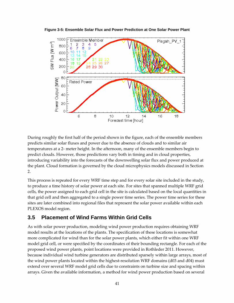
41
Figure 3-5: Ensemble Solar Flux and Power Prediction at One Solar Power Plant
During roughly the first half of the period shown in the figure, each of the ensemble members predicts similar solar fluxes and power due to the absence of clouds and to similar air temperatures at a 2- meter height. In the afternoon, many of the ensemble members begin to predict clouds. However, those predictions vary both in timing and in cloud properties, introducing variability into the forecasts of the downwelling solar flux and power produced at the plant. Cloud formation is governed by the cloud microphysics models discussed in Section 2.
This process is repeated for every WRF time step and for every solar site included in the study, to produce a time history of solar power at each site. For sites that spanned multiple WRF grid cells, the power assigned to each grid cell in the site is calculated based on the local quantities in that grid cell and then aggregated to a single power time series. The power time series for these sites are later combined into regional files that represent the solar power available within each PLEXOS model region.
3.5 Placement of Wind Farms Within Grid Cells As with solar power production, modeling wind power production requires obtaining WRF model results at the locations of the plants. The specification of these locations is somewhat more complicated for wind than for the solar power plants, which either fit within one WRF model grid cell, or were specified by the coordinates of their bounding rectangle. For each of the proposed wind power plants, point locations were provided in Rothleder 2011. However, because individual wind turbine generators are distributed sparsely within large arrays, most of the wind power plants located within the highest-resolution WRF domains (d03 and d04) must extend over several WRF model grid cells due to constraints on turbine size and spacing within arrays. Given the available information, a method for wind power production based on several

42
heuristics was developed. These heuristics are described for the Tehachapi, California, region, which provides examples of the types of decisions that must be made in assigning WRF model grid cells to wind power plants.
Figure 3-6 depicts the set of modeled wind power production plants located near Tehachapi. The green shading depicts terrain height, the colored squares show the locations of the WRF model grid cells assigned to various wind power plants, and the colored dots indicate an estimate of wind power production potential from a resource characterization study conducted by 3TIER Corporation (3TIER, 2010).
Figure 3-6: Modeled Wind Power Plants Near Tehachapi, California
The figure shows one existing and four proposed wind power plants near Tehachapi. T_2005, shown by the purple squares, denotes the existing Tehachapi wind power plant as of 2005. The grid cells comprising T_2005 were obtained by visual inspection of Google Earth images. The white polygon denoted T_2012 describes the approximate perimeter of the wind power plant area as of 2012. Most of the area within T_2012 contains predominantly older, smaller turbine vintages, characteristic of technology developed before 2005. However, the southeastern portion (lower right in the figure), contains newer, larger turbines. This analysis enables demarcation of the T_2005 perimeter within T_2012.
The blue asterisks in the figure denote the point locations of the proposed wind power plants specified in Rothleder 2011. The location for proposed plant Tehachapi_W2 (T_W2) coincides with grid cells already allocated to T_2005. Given the observed development using newer, larger turbines within T_2012, adjacent to T_2005, T_W2 was allocated the grid cells within T_2012 not allocated to T_2005, as shown by the blue squares.

43
The blue squares representing T_W2 extend beyond the perimeter of T_2012. This is due to the manner in which the number of WRF grid cells to allocate to T_W2 was determined. Following the method outlined in the 3TIER report, it was assumed that all proposed development will use the Vestas V90 3.0 MW turbine. These turbines will be placed in arrays with an average spacing of 10D and 4D in the streamwise and spanwise directions, respectively, where D refers to the 90 meter rotor diameter. With this spacing, each 9 km2 WRF model grid cell will contain, on average, about 27.8 turbines, generating roughly 83.3 MW of power.
For each proposed wind plant, the total MW capacity given in Rothleder 2011 is divided by 83.3 to determine the number of grid cells the farm would occupy. If a fractional grid cell remains after this calculation, sufficient capacity is allocated to an additional grid cell so that the total capacity of the wind plant matches the capacity given in the reference.
For T_2005, as well as each of the other existing (as of 2005) wind power plants, the number of MW per grid cell is obtained by tiling (approximately) the observed extent of the plant area, as obtained from Google Earth imagery, and dividing the total number of MW for each plant by the number of grid cells used for the tiling. Because all these plants use smaller, less powerful turbines than the V90, placing 27.8 turbines in each grid cell would exceed the total plant output. Instead, the total power output is divided by the total number of grid cells required to tile it, and the number of V90 turbines required to satisfy that amount is assigned to each grid cell8F
9.
The MW for each of the existing wind plants was estimated using a combination of PLEXOS existing wind power production files and information obtained from an Energy Commission study (CEC 2005), which identified all of the existing wind power generation facilities as of 2003. The PLEXOS existing wind production files specified values of 882 MW and 1166 MW for the PGE and SCE regions, respectively. The major existing wind production plants operating within each of these regions in 2005 were assumed the same as those identified within the 2003 Energy Commission study. As of 2003, these included Altamont (562 MW) and Solano (165 MW), within the PGE region, and Tehachapi (710 MW) and San Gorgonio (359 MW), within the SCE region. The other smaller plants (Pacheco, Orange, and San Diego, with production capacities of 16 MW, 36 MW and 4 MW, respectively, as of 2003) were omitted, as those contributed only a few percentage points of the combined production of the larger plants in each region.
The relative amounts of power assigned to each of the two plants within each utility region were obtained by scaling up the 2003 production amounts to the values of the PLEXOS existing wind production files, such that the proportion of power produced by each plant in 2005 relative to the total within each region matched the 2003 values. MW values assigned are shown in Appendix A.
9 Because much of the existing wind power uses turbines that are smaller and closer to the ground, use of the V90, which uses the wind speed at 90 m above the surface, could result in overestimation of power from these plants.

44
An additional consideration in allocating WRF model grid cells to a particular plant is the estimate of capacity factors, which are identified by the colored circles in Figure 3-6. The capacity factors were determined using a combination of high-resolution mesoscale model simulations and statistical techniques, as discussed in the 3TIER report. Red, orange, yellow, and green circles denote capacity factors of greater than 40 percent, 40-35 percent, 35-30 percent, and 30-25 percent, respectively.
While the projected capacity factors provide some useful guidance for potential development areas, careful analysis reveals limitations of the dataset and difficulties in interpretation. For example, much of T_2005 is characterized as favorable for development, while little of T_W2 is favorable. However, T_W2 was recently developed. Because T_2005 consists of many older turbines, this may imply that much of the area is a candidate for redevelopment using modern turbines, while T_W2 is not because it was recently developed using newer, larger turbines. It was also noted that the area immediately northeast of T_2012 shown to be favorable for development includes the city of Mojave, California, which would preclude significant development.
The locations of all of the proposed wind power plants are associated with data from the 3TIER report representing the 30-35 percent category for projected capacity factors. The research team interpreted such a choice as an attempt to be conservative and adopted that guideline as well. While the allocation of WRF model grid cells to T_W2 required unique treatment (as described above), allocations of grid cells to T_W1, T_W3 and T_W4 were determined using the following guidelines:
i) Grid cells comprising each plant use the coordinates given in Rothleder 2011.
ii) Grid cells comprising each plant must be adjacent to one another.
iii) Grid cells comprising each plant are guided by conservative values of the capacity factor (30-35 percent) given in the 3TIER report, unless siting conflicts are identified.
The associations of WRF model grid cells with the other wind projects within the 3 km WRF domains (d03 and d04) were undertaken in a similar fashion to those used for the Tehachapi region. In some regions that include water, an additional requirement that wind projects be located on land was imposed. Like the Tehachapi region, the Solano region also contains a combination of existing and proposed development. The Altamont and San Gorgonio wind power plants include only existing development. The remaining plants consist entirely of proposed development.
Each of the wind power plants located outside the 3 km WRF domains (d03 and d04) is able to produce the capacities from within the footprint of the single WRF model grid cell containing the plant due to the larger grid cell footprints on the coarser-resolution domains. The names, locations, and other relevant information from each of the wind power plants are provided in Appendix A.

45
3.6 Calculation of Wind Power From Wind Speed After the WRF model grid cells associated with each wind power plant are identified, the wind speed is computed from the horizontal velocity components at each of those grid cells. The wind speeds are interpolated to 80 m, the hub height of the V90 turbine, for which the manufacturer’s power curve is calibrated.
The power is obtained using a piecewise polynomial function approximation to the manufacturer’s power curve9F
10. The power model returns nonzero power for wind speeds above the “cut in” wind speed of 3.0 m/sec and below the “cut out” wind speed of 25 m/sec. For wind speeds between 3.0 m/sec and 15.0 m/sec, the power function consists of a sixth-degree polynomial curve fit to the manufacturer’s power curve, which increases from 0 to 3 MW over this range. For wind speeds between 15.0 m/sec and 25 m/sec, the power output is 3 MW. Power falls to zero for wind speeds in excess of 25 m/sec. The power curve is shown in Figure 3.7.
Figure 3-7: Power Curve for Vestas V90 Wind Turbine
Source: Vestas Wind Systems A/S
This value of power returned is then multiplied by the total number of turbines specified within the given model grid cell. Finally, all grid cells comprising the plant are summed to compute the total wind power produced at each plant.
Figure 3-8 shows an example of the predicted wind speed and corresponding power generated at one of the proposed wind power plants (Tehachapi_W2; T_W2 in Figure 3-6). Time trajectories of wind speed (top) and power (bottom) are shown from an ensemble of 30 WRF
10 No models for the effects of atmospheric stability, temperature, or wake effects were implemented for this study. Researchers applied a simple reduction of 5 percent of the power obtained from the power curve to account for these unknowns, and to be conservative. Models for these effects could be incorporated to the existing analysis framework.

46
simulations, with colored lines in each panel depicting trajectories from each of the 30 ensemble members. The rated power of the plant is depicted by the dashed horizontal line in the lower panel of the figure.
Figure 3-8: Ensemble Wind Speed and Power Prediction at One Wind Power Plant
The figure shows that each of the ensemble members predicts a similar series of increases and decreases in wind speed and power throughout the period. However, the magnitude, slope, and timing of the ramps vary among the ensemble members and increasingly so for later times within the forecast window. Toward the end of the forecast period, the timing of the wind ramp varies by over three hours among the trajectories in the ensemble. Hence, the ensemble estimates the uncertainty in timing of wind ramp events – information that would be useful to system operators.
3.7 Aggregation of Wind and Solar Sites Into PLEXOS Model Regions Although researchers attempted to mirror California ISO’s accumulation of sites as closely as possible, Rothleder 2011 does not specify which wind and solar sites are assigned to which WECC region in the PLEXOS model. For many of the sites, the assignment was clear. For others, particularly those in California, it was not always clear to which region a particular site should be assigned. In some cases, it appears that a site was split between multiple regions in the PLEXOS model. These assignments of capacities to the different regions in California will have little effect on the overall California ISO net load, so approximations were used.
The team used a combination of geographic locations and capacities to determine which sites to assign to which regions. They also used the total capacity assigned to each region based on the dispatch files that were included with the California ISO High Load model. The longitude and latitudes of each project were mapped using Google Maps, as shown by the elliptical markers in

47
Figure 3-9. This allowed the team to easily see the locations of various projects. They then made a list of the various wind and solar buildout files that were associated with each region and found the maximum MW of generation during the entire year for each file, which was used as a proxy for capacity. These files are broken down by region and separated into wind, large-scale PV, solar thermal, small scale PV, and distributed solar. Distributed solar resources were assumed to be uniformly spread over the rectangles shown in the figures.
Figure 3-9: Map of All Wind and Solar Projects
For each category of wind and solar resource, projects were assigned to regions based on geographical proximity and project rating in such a way that the total capacity of the included projects roughly matched the maximum power production in the corresponding file. Some sites needed to be split among multiple regions to create regional aggregations that summed to the correct regional capacity. The simplest example of this is the “distributed solar” category, which was represented by five rectangles in California, each containing 349.9 MW (a total of 1749.5 MW), according to Rothleder 2011, Appendix 2. However, these sites were gathered into six distributed solar files associated with the regions designated LDWP, PGE_BAY, PGE_VLY, SCE, SDGE, and SMUD, whose maximum generation levels were 178.4, 349.9, 552.2, 480, 160, and 27.3 MW, respectively (a total of 1747.8 MW). Thus, it was necessary to use geographical information to assign fractions of each distributed solar rectangle to the appropriate regional combined files.

48
The mapping of sites in Appendix A to PLEXOS files of fixed dispatch generation levels is given in Table A-6 through Table A-10. The columns in each table represent a PLEXOS input file, and the rows represent wind or solar sites. The numbers in the tables represent the fraction of a given site (row) that is assigned to a given file (column).

49
CHAPTER 4: Load Data Load forecasts developed to support California ISO’s 33 percent renewable integration study (Rothleder 2011) were acquired for use in this study. Because the California ISO study did not include the use of weather ensembles and related effects on renewable generation and load, some adjustments to load were necessary. In addition, several consistency checks were conducted to confirm the applicability of in- and out-of-state load data as described in the later sections of this chapter.
4.1 Load Adjustments for Temperature The PLEXOS model used in the analysis requires load data for every WECC region at two time scales. A set of day-ahead hourly load forecasts are required for the stochastic unit commitment algorithm in PLEXOS, and five-minute average loads are required for the economic dispatch and short-term unit commitment algorithm.
The temperatures in each of the 30 hypothetical weather trajectories generated by WFR with multiphysics modeling can influence the loads. To produce consistent pairs of renewable generation and load trajectories, the team adjusted the base case load in California ISO’s PLEXOS model to reflect the deviations from the realized temperatures associated with that base case load. This temperature adjustment was performed only for the loads in California. Out-of-state loads were taken directly from the California ISO PLEXOS model.
This general approach used for these load adjustments is as follows:
1) Use historical load data to calibrate a set of equations that capture how loads in each of the regions in each hour of the day change with temperature.
2) Calculate an average temperature for each period, each region, and each of the 30 trajectories in the weather ensemble
3) For each weather trajectory and region, calculate the temperature difference between the average temperature for that trajectory and the realized temperatures corresponding to 2020 loads (delta T for trajectory and period).10F
11
4) Use the delta T term and the equations from Step 1 to calculate an adjustment to load for each period, trajectory, and region.
11 The energy in each of the ensemble members may be different from the energy assumed in the base case scenario because the temperatures differ from ensemble member to ensemble member. However, the dispatch over the operating day is done using the synthetic observations, which attempt to reflect base case loads.

50
4.1.1 Generation of Load Adjustment Equations The weather trajectories generated by the multiphysics model vary in the prediction of local temperature around California. Because day-ahead load forecasting is a strong function of day-ahead temperature predictions, the temperatures from the weather trajectories was used to create day-ahead load forecasts that corresponded to each trajectory. In this way, researchers were able to use stochastic optimization to make day-ahead unit commitment decisions based on not only the predicted availability of nondispatchable resources, but based on the predicted load.
When California ISO makes day-ahead load forecasts, it uses a load-weighted temperature, which is a weighted average of the temperature forecasts at various locations. This process was mimicked to obtain the load forecasts for each weather trajectory. In this analysis researchers used historical load and temperature data to find the ratio of the change in load, ΔL, to the change in load-weighted temperature, ΔT. This ratio, ΔL/ΔT was found to be a function of temperature and hour of the day. Researchers did not find that it varied much by day of the week or season, though the absolute load levels do, of course, vary by day of week and season.
The team then found the difference between the weighted temperature in a single trajectory and a baseline temperature. This difference, ΔT, was then used in conjunction with the previously calculated ΔL/ΔT to find the change in load, ΔL, from the baseline load. For this study, the pseudo-observation weather simulation was used, which is “nudged” to agree with local weather measurements, to calculate the baseline temperature. The baseline load was taken from California ISO’s PLEXOS model. These hourly loads, generated by California ISO, were obtained by applying a scaling factor to the 2005 California historical load and then partitioning the scaled load for the entire state among the eight Californian regions defined in the PLEXOS model (PGE_BAY, PGE_VALLEY, SCE, SDGE, SMUD, LADWP, IID, and TIDC).
4.1.2 Calculation of ΔL/ΔT To determine ΔL/ΔT, the research team used historical hourly load data from the California ISO Oasis database and weather station data from a set of stations corresponding to load centers in California. Hourly load data were segregated by day of the week, hour of the day, and time of year. Each subset of data was plotted as a function of weighted temperature, and a second order polynomial was fit to the data. The derivative of this polynomial was used to determine ΔL/ΔT. Finally, the estimates of ΔL/ΔT at various temperatures for all data sets corresponding to a single hour of the day were plotted as a function of temperature and another second order polynomial fit was established through these data to determine ΔL/ΔT as a function of temperature and hour of the day. In this section, each step is explained with examples.
Figure 4-1 shows load as a function of weighted temperature for every hour of 2005 for all of California. While a distinction is made between weekend and weekday loads, the spread in load for a given temperature is clearly quite large.

51
Figure 4-1: Load Versus Temperature for California ISO
40 50 60 70 80 90 100 11020
25
30
35
40
45
50
Temperature (F)
Load
(GW
)
oad s e pe atu e o C
WeekdayWeekend
To develop a more precise estimate, the load and temperature data were divided into groups by year, time of year (into six 2-month groupings), day of the week, and hour of the day. Holidays were excluded from the data. This aggregation results in between 6 and 10 data points per second order fit. For example, one data set was the hourly load and temperature from every Thursday at 10 a.m. in January and February. This method allowed the research team to reduce the data, establish trends, and determine which parameters (time of day, time of year, and so forth) have the most effect on the ΔL/ΔT ratio. The quantity ΔL/ΔT can be extracted from these polynomial fits simply by taking the derivative of load with respect to temperature: ΔL/ΔT ≈ dL/dT.
An example set of fits is shown Figure 4-2. The six data sets and polynomial fits in the figure correspond to the six bimonthly periods for a single hour and weekday. Based on the fits to these data sets and similar fits for other days of the week and times of day, it was determined that ΔL/ΔT did not have a strong dependence on time of year, besides for the obvious dependence on temperature (which, in turn, depends on time of year). The differences in ΔL/ΔT as a function of time of year were not large enough relative to the errors in the fit to justify a separate analysis for different times of year. Thus, all values of ΔL/ΔT obtained from fits at a given temperature were considered when calculating the final value of ΔL/ΔT to be used in the load adjustment analysis. The actual load levels did vary with the season, so separate fits to the seasonal data sets were warranted. In total, 1,008 such curves were developed and used for this analysis (24 hours x 7 days x 6 bimonthly periods). The years 2001 through 2011 were used for

52
the analysis. The difference between years was not deemed significant, so all years were combined into a single data set.
Figure 4-2: Second Order Polynomial Fit for Single Hour and Weekday
50 55 60 65 70 75 80 85 90 95 10025
30
35
40
45
50y
Temperature(F)
Pow
er (
GW
)
ActualFit
A typical standard deviation on the polynomial fits of the load versus temperature shown in the figure is nearly 500 MW. However, the standard deviation varies over a day. A plot of the approximate fitting errors is shown in Figure 4-3. As might be expected, the standard deviation of the error increases with higher loads. The standard deviation is about 1.5 to 2 percent of the load.
Figure 4-3: Standard Deviation of Prediction Error
0 5 10 15 20 25300
350
400
450
500
550
600
650
700
750
800Stdev of fit
Hour
Erro
r(MW
)

53
Several additional weather factors can play a role on the load, such as cloud cover, precipitation, and humidity. However, these additional factors were not incorporated in the analysis.
The ratio ΔL/ΔT was calculated independently for each hour of the day, day of the week, season, and year. Based on these calculations, it was determined that ΔL/ΔT did not have a strong dependence on day of the week, season, or year, even though the load levels depend on these parameters. Thus, when making the final determination of ΔL/ΔT, all the ΔL/ΔT data points for each hour of the day were aggregated. Figure 4-4 shows a clear relationship between ΔL/ΔT and temperature. As the temperature increases, the sensitivity of the load to temperature increases, with the minimum sensitivity of around 62 °F. Below this temperature the load decreases as temperature increases. Above 62 °F, the load increases as temperature increases. At 100 °F, a 1 °F increase in temperature could cause an estimated 1 GW increase in load. Thus, temperature forecast errors can play a significant role in the accuracy of the load forecast.
Figure 4-4: Fit of ΔLoad/ΔTemp Data
50 60 70 80 90 100-0.5
0
0.5
1
1.5
Temperature (°F)
∆L
/ ∆T
(GW
/ °F
SunMonTueWedThurFriSat
The value of interest for this study is the ΔL/ΔT term or the change in load for a degree change in temperature. This quantity can be approximated by fitting another second order polynomial to the combined values of ΔL/ΔT for all times of year and all days of the week. A curve of ΔL/ΔT as a function of temperature was fit for each hour of the day. The comparison of the fit when separated by days of the week indicated no significant change either by season or day of the week. The loads themselves change significantly when accounting for those factors;

54
however, the sensitivity of load to temperature only marginally depends on day of the week. To simplify calculations, the only factor considered was the hour of the day.
A contour plot of the resulting ΔL/ΔT estimates is shown in Figure 4-5. The figure shows increasing sensitivity to temperature for the morning hours and evenings when the temperature is high and relatively constant sensitivity during the work day. The units of the color bar are in GW per degree Fahrenheit.
Figure 4-5: ΔL/ΔT Versus Temperature and Hour of the Day
Time of Day(HR)
Tem
pera
ture
(F)
y
5 10 15 2030
40
50
60
70
80
90
100
110
-0.2
0
0.2
0.4
0.6
0.8
1
1.2
1.4
This analysis provides a set of equations used to calculate the sensitivity of changes in load to changes in temperature for a given time of day and temperature. The load sensitivity parameters were estimated for each region based on the regional load-weighted temperatures.
The load sensitivity parameters are used to estimate how the load would have behaved for each member of the ensemble of weather forecasts by applying them to the load data from the California ISO PLEXOS model. The weather data from the pseudo observations were used to establish the base temperature. The temperature difference of the individual trajectories from the pseudo observations is used as the ΔT in the computation.
4.1.3 Calculation of a Load-Weighted Temperature for Each California Region The calculation of the load-weighted temperature is derived from regional load ratios established by California ISO for use in its load forecasting system. The weights are associated

55
with weather stations located around the state in key load areas. Given the variability of the load between days, only an approximate regional temperature is needed; so the simple approximation reduces computation time without significantly increasing error.
In the WRF output, each station is associated with a position. For each trajectory, the temperature of the grid cell associated with a stations position is multiplied by the respective regional weight and summed to create a regional load-weighted temperature. Several regions such as TID, SMUD, and LADWP contain only a single station; thus, the temperature at that station is taken as the average temperature.
4.1.4 Calculation of Load Changes for Each Trajectory The ΔL/ΔT analysis produces a set of equations for each region based on time of day. As discussed, the regional ΔL/ΔT is estimated using the derivative dL/dT, which is computed as follows:
Where A, B, and C are the parameters obtained from the data regression, such as the one shown in Figure 4.4. These parameters are computed for each region and for each hour of the day. The variable T is the load-weighted temperature for a specific region measured in degrees Fahrenheit. The computation of the ΔL involves integrating the ΔL/ΔT equation over the temperature difference. This can be evaluated in closed form resulting in the following equation:
In this equation, T_i is the load-weighted regional average temperature for trajectory I, and T_b is the base case temperature corresponding to the load that is being adjusted. This adjustment is performed on an hourly interval to adjust the load to match the weather in the trajectories that are used for day-ahead unit commitment.
4.1.5 PLEXOS Load Profiles by Region The California ISO PLEXOS model includes hourly load data for each of the eight California regions. These regions were given the same load shape, with a simple scalar multiplier differentiating the loads in each region.
In addition to the hourly regional load data, the model requires five-minute regional load data for economic dispatch in PLEXOS. For this, California ISO’s dataset of one-minute load for the entire state for 2020 was used. This one-minute dataset, which uses a 2005 date time base, is shifted in time to match the 2020 time base. It is then averaged over five-minute periods to obtain a five-minute dataset. Filtering is performed on the dataset to remove occasional large spikes in load, which are likely artifacts of failures and other events that may have actually occurred in 2005. This filtered dataset is then divided into the eight California regions using the same scalar multipliers that California ISO used to produce the hourly data.

56
In obtaining the five-minute data, it was discovered that some inconsistencies exist between the five-minute data set and the hourly dataset, particularly at night where the two load profiles may differ by up to 300 MW. To keep the two datasets consistent, the hourly data were regenerated using the five-minute data. Thus, the hourly loads in the model are slightly different from those used in the model built by California ISO11F
12. However, it is not expected that these differences in load will affect the results significantly, given that they occur at night.
The final step in generating the hourly loads is to adjust the load based on the temperature in each trajectory. This is done by regional temperature so that the final regional load shapes are slightly different from one another.
4.2 Example Net Load Data The methods described in this chapter were used to compute 30 member ensembles of net loads (gross load – renewable generation) in California for California ISO’s Trajectory and High Load cases. Example results for the week of April 5-11, 2020, are shown in Figure 4-6.
Figure 4-6: Ensemble of Net Loads in California for the Week of April 5-11, 2020
The noon load for many days is as low as the minimum load that is usually realized at about 3 a.m. Also, there are morning and evening peaks with high ramp rates preceding them. This increased variability in load can be attributed to the large deployment of solar generation resources that have maximum output at noon. Unfortunately, during the winter and spring months, solar generation typically comes on-line too late in the morning to reduce the morning net load ramp and goes off line too early in the evening to reduce the evening peak. April 9 appears to be a day with a large dispersion in the forecast ensemble. The trajectories for this day are shown in Figure 4-7. 12 Designated as Hi Load+LCR+WECCAS by California ISO in the model.

57
Figure 4-7: Ensemble of Net Loads in California for April 9, 2020
As indicated by the data in the figure, there is significant uncertainty in the net load in the early afternoon. The timing and magnitude of a weather front driving wind and solar generation may be contributing to the uncertainty on this day. Additional examples of net load trajectories are shown in Appendix B.

58
CHAPTER 5: Clustering and Selection of Trajectories The previous chapters described how the WRF and multiphysics models generate an ensemble of 30 weather trajectories that are converted to net load using models of renewable resources and perturbations of load caused by the weather. Conceptually, these 30 net load trajectories could be passed to a production simulation code to perform stochastic unit commitment optimization for the day-ahead market. As discussed previously, the production simulation model used for this study is California ISO’s 42 node, 104 line, and 2,400 generator PLEXOS model of the WECC (Rothleder 2011). Experiments with this PLEXOS model indicate that run time and memory usage become excessive when more than six net load trajectories are included in the problem. The computation times for problems with various numbers of net load trajectories are shown in Figure 5-1.
Figure 5-1: Computation Time Versus Number of Net Load Trajectories
As indicated in the figure, solution of the day-ahead stochastic unit commitment problem with six trajectories requires roughly 2 hours of computation time. Increasing the number of trajectories to 12 increases the solution time to 7 hours. The CPLEX solver failed to find a feasible solution with 20 trajectories after 33 hours of computation time. Therefore, it was necessary to reduce the ensemble of 30 trajectories to a computationally feasible set of five or six that represent the uncertainty and variability in renewable generation and load.
The general concept used for reduction of the ensemble is to include a few trajectories that stress the system (for example, high net load ramp rate), each with an appropriate probability weight (such as, 1/30 for a single selected trajectory). Statistical clustering methods are then used to gather the remaining trajectories into like groups and to select a representative trajectory from each group. This process reduces the 30 trajectories to 5 or 6. Because 30

59
trajectories are sampled and the outlier of this sample is selected (top 3.3 percent of the sample), the range of uncertainty captured by this process is conceptually similar to the 95 percent confidence limits used in previous California ISO renewable integration studies (California ISO 2010, Rothleder 2011).
Statistical clustering methods group observations (scalar- or vector-valued) into clusters, with each cluster consisting of observations that are more similar to one another than to observations in other clusters with regard to some specified characteristics. These characteristics are relevant summary features of each observation. In this case, the observations are the 30 individual 24-hour net load trajectories, and the features are quantities that the research team deems important for capturing the amount of stress any particular trajectory may have on the system. The goal is to use a clustering method to obtain six or fewer clusters and then select one representative trajectory from each of the clusters. By design, each trajectory selected in such a way represents the respective cluster in terms of the specified features. A weight proportional to the size of the cluster is then assigned to each chosen trajectory, and these trajectories, along with associated weights, can then be used as inputs to the stochastic unit commitment optimization algorithm in the PLEXOS model.
K-means clustering (Hartigan 1979) is one of the most commonly used clustering algorithms due to simplicity and effectiveness. It assigns each observation to the cluster whose mean is closest to the observation. (This is a particular way to measure similarity within a cluster.) K-means is an iterative method because once an observation is assigned to a cluster (there are several schemes to initialize the clusters), the mean of that cluster is recomputed, and cluster assignment is updated. This is repeated until cluster assignment no longer changes from one iteration of the algorithm to the next.
5.1 Key Features of Net Load Trajectories A previous California ISO renewable integration study (California ISO 2011, pg. 84) identified features of interesting periods that were selected for more detailed analysis. In that study, days with large net load ramps were considered for additional stochastic analysis. Accordingly, in this study two features of net load trajectories were used to characterize and cluster the data:
• Maximum four-hour net load ramp rate (max change in MW for a four hour period for the day)
• Maximum daily net load (MW)
The four-hour period specified for the first feature was based upon examination of the data – many of the large-scale net load ramp events occurred over roughly a 4-hour period. The second feature reflects the total amount of fossil and hydro unit dispatch required to cover the peak load during the day. Only positive net loads ramps are considered because they generally involve higher ramp rates and stress the system more than the negative net load ramps.

60
5.2 Trajectory Reduction Results The features described in the previous section were computed for each of the 30 trajectories in a given day’s ensemble. To ensure that the trajectories that are expected to stress the system the most in that 24-hour period are included in the final set of five or six, the trajectories with the extreme value of each feature were automatically selected in the final set. This selection provided one or two trajectories to be included in the set. (One trajectory will result from this step if the same trajectory is extreme in both features in that 24-hour period.) The other four or five trajectories were identified by clustering the remaining 28-30 trajectories using the K-means clustering method described above.
The trajectory selection method is illustrated in Figure 5-2, which shows the results for April 9, 2020, for selection of six trajectories. The 30 net load trajectories in the ensemble are characterized in terms of the two features mentioned earlier: the maximum net load (x axis) and the maximum 4-hour net load ramp rate (y axis).
Figure 5-2: Clustering of April 9, 2020, Trajectories
The trajectory with the largest maximum 4-hour ramp is denoted in the figure by the orange star at the top of the figure. This trajectory is selected as one of the six trajectories (as indicated by the star icon). Similarly, at the lower right-hand side of the figure, the magenta star

61
corresponds to the trajectory with the largest maximum net load and is identified as a singleton cluster and a selected trajectory. Each of these was assigned a probability weight of one divided by the total number of trajectories, or 1/30. The remaining 28 trajectories in the figure were clustered into four groups with a K-means clustering algorithm. These are color-coded in the figure to indicate the membership in one of the four clusters. The computed centroid of each cluster is indicated by “x” icons. As a final step, the trajectory belonging to the cluster that is the closest to the centroid of the cluster is selected for inclusion in the final set of six trajectories. Each of the four trajectories selected via clustering was assigned a probability weight equal to the number of points in the cluster it was chosen from divided by the number of trajectories. Thus, the trajectories indicated by the red, turquoise, green, and blue circle and star received weights of 9/30, 7/30, 9/30 and 3/30, respectively.
The result of the above process for April 9, 2020, is shown in Figure 5-3. The figure shows the original 30 trajectories in the ensemble (in gray) and the 6 trajectories that were selected (each in color corresponding to the color of the cluster in Figure 5-2). As indicated in the figure, the trajectory with the largest net load ramp rate is selected. It appears as the orange trajectory line on the bottom boundary of the envelope at 15:00 hours. The trajectory with the largest maximum 4-hour ramp rate is also shown in the figure (magenta). The remaining 28 trajectories were then grouped using the K-means clustering algorithm, and 4 trajectories were selected from these, as indicated in the figure. The width of each trajectory line corresponds to the probability weight assigned to the trajectory (which is equal to the number of trajectories in the cluster divided by 30), as described above. This trajectory aggregation approach was applied to the data for the months of February, April, August, and November, and the results for one selected week from each of these months are shown in Appendix B.

62
Figure 5-3: Trajectories Selected to Represent the 30-Member Ensemble for April 9, 2020
In addition to the maximum 4-hour ramp and maximum net load, the team also investigated two other variables as possible features in trajectory reduction. One was the start time of the maximum 4-hour ramp because including this feature would help ensure that trajectories with early large ramps would be included in the final set of six trajectories. However, it was found that on almost all days in April and August (the first two months were considered), the original 30 trajectories exhibited little variability in this feature: on 67 percent of days in April and 62 percent of days in August, the range in the start times was at most 3 hours. (The start times were identical for all the trajectories on 33 percent and 24 percent of days in April and August, respectively.) Therefore, the team concluded that instead of using the start time of the max 4- hour ramp as a feature in clustering, it would be more practical to verify that it is well represented among the selected trajectories (obtained via the procedure described above) relative to the original 30 trajectories.
Hence, Kolmogorov-Smirnov test statistics (Corder 2009) were computed to compare the distributions of the start times of the maximum 4- hour ramps among the selected and original trajectories for all days in all four months and found no statistically significant differences

63
among these for any of those days. It was concluded that the range of possible ramp start times is well represented by the selected trajectories.
The team also considered clustering on the net load at the hour of maximum variability in net load among the trajectories throughout the day. Its motivation was to capture significant differences among the trajectories. However, this quantity did not correlate highly with any of the features that would be considered stressors to the system, such as long or large ramps or high net loads. In addition, the relative ranking of a particular trajectory in terms of net load is not consistent throughout the day: Trajectories that tend to have higher net loads at a given hour are not more likely to have higher net loads at other hours (that is, net load trajectories cross each other frequently during the day). This further convinced researchers that the net load at the hour of maximum intertrajectory variability in net loads is not a useful clustering feature.
5.3 Approaches Used by Other Researchers Other approaches to reducing the number of trajectories to a feasible number have been proposed. For example, previous research (Papavasiliou 2012) on high-performance computing (HPC) systems at LLNL demonstrated that importance sampling techniques were effective for reducing 1,000 trajectories to 10 that captured the uncertainty and variability in renewable generation. In that work, the importance density and weights are determined using the cost of each trajectory, so it is necessary to first use duality-based optimization to reduce the number of trajectories.
Researchers at Risoe National Laboratory in Denmark have also developed methods for gathering renewable generation trajectories (Meibom 2006). Their methods are based on trajectory reduction algorithms proposed in Dupacova 2003, which, in turn, cluster trajectories using the Kantorovich distance metric for measuring the dissimilarity between probability distributions. They demonstrated the method on a small-scale, 23-generator model of the grid in Northern Europe.
These two approaches share some common characteristics with the K-means clustering method presented earlier in this chapter. However, the latter has the advantages of being simpler and explicitly using trajectory features that are expected to stress the system.

64
CHAPTER 6: Production Simulation Modeling This chapter depicts the production simulation model that takes the net load scenarios as input and schedules the fossil fuel, hydroelectric, storage, and demand response resources to meet demand at minimum cost. An iterative application of the production simulation model with different resource capacities is also described. This process shows how the marginal value of a resource declines as more of it is added. Finally, the real-time electromechanical simulation model that is used to evaluate regulation performance and system stability is described.
6.1 Analysis Process The analysis is structured to assess the value and feasibility of using demand response and storage to provide regulation, load following, and energy arbitrage in a California ISO market with 33 percent renewable generation. The overall flow of the analysis is shown in Figure 6.1. The blue processes in the figure refer to the weather and load modeling procedures, which are described in Chapters 2 through 5. This chapter describes the processes in the yellow boxes, including the production simulation model with unit commitment (UC) and economic dispatch (ED) procedures, and the process in the green box that refers to checks of system stability to confirm that the results of the simulation model meet system stability requirements.
Figure 6-1: Analysis Process

65
California ISO system loads must be met by some combination of intermittent nondispatchable generators such as wind and solar, hydroelectric generators, fossil fuel generators, energy storage resources, demand response, and imports from other states in the Western Interconnect. The production simulation generation from nondispatchable renewable generators is assumed to be fixed. (They are not curtailed.) The renewable generation and gross loads are passed the PLEXOS production simulation model, which co-optimizes energy and ancillary services.
As indicated in the figure, the production simulation model uses a two-stage optimization procedure to find the least-cost way to operate the system. The first stage finds an optimal unit commitment (on or off state of the resource) schedule for fast- and slow-start units using hourly forecasts of net load. The second stage assumes the unit commitment states of slow start units are fixed and finds an optimal unit commitment schedule for fast-start units and economic dispatch (power level) schedule for all units that minimizes overall cost of meeting system load and reliability constraints. All resources and the corresponding variable costs, including demand response and storage, are taken into consideration by the optimization code. The role and value of demand response and storage depend strongly on the set of conventional units that have been committed and dispatched at any given time.
As shown in the figure, the output of the production simulation model is the system state (generator output, hydro reservoir and other storage levels) at each time interval in the year. In addition, the production simulation model provides the value and usage of demand response and storage resources at each period. The value estimate provided by the model is based upon the resources that demand response and storage displace. The output of the production simulation model is also provided to a system stability analysis code that computes response of the system to potential transients, such as loss of a generator or transmission line. This response must meet stability conditions imposed by system regulators.
6.1.1 Storage and Demand Response Capacities The process in the figure shows an analysis loop in which the capacities of demand response and storage can be changed and the production simulation model rerun. A key objective of this analysis is to provide insight to policy makers regarding goals for developing storage and demand response capacity in the California ISO system. An assessment of the economic motivations to developers can inform policy makers.
Consider the economic incentives for deployment of the first MW of storage capacity. This unit could charge during periods when prices are at a daily minimum and discharge when prices are at the daily peak. This would result in net revenues12F
13 for that first unit of capacity. The second unit of capacity added would have to pay a higher price for energy to charge and would receive a lower price for the energy discharged. The net revenue would be lower than the net revenue of the first unit of capacity. Net revenues from subsequent additions of capacity would be lower still. This decrease in net revenues, or marginal values, of additional capacity is illustrated in Figure 6-2.
13 Revenues from sale of electricity less costs of electricity purchases and variable O&M costs. Capital and fixed O&M costs are not taken into account in the production simulation model.

66
Figure 6-2: Marginal Value of Storage
The figure shows that the marginal value of each MW of storage capacity decreases as more MW capacity is built. On the left part of the curve, the high marginal net revenues are sufficient to justify the capital investment in storage capacity. As MW quantity increases and marginal net revenue decreases, it eventually becomes uneconomical to make the next marginal investment in capacity—the marginal revenue from an additional unit of capacity will not justify the capital cost of the capacity. This occurs at the “break even” point in the figure. This point might be a reasonable policy goal that is consistent with investor and ratepayer needs. Thus, this curve can guide policy makers and resource developers when making goals and investment plans. In Chapters 8 and 9, curves for various storage and demand response technologies were constructed using results of the production simulation model. In a fully optimized system, storage capacity is added up to the point where the marginal value is equal to the marginal cost13F
14.
6.2 Production Simulation Modeling With PLEXOS Software The PLEXOS software is used to conduct production simulation analysis (Plexos 2012). A model developed by California ISO to analyze its High Load scenario was the starting point for the model (Rothleder 2011). Two new features of the PLEXOS software were used for the analysis – stochastic unit commitment and interleaved timescales.
14 Lamont, A. D., “Assessing the Economic Value and Optimal Structure of Large-Scale Electricity Storage,” IEEE Transactions on Power Systems, Vol. 28, No. 2 (May 2013).
Quantity (MW storage)
Marginal value of storage (net revenue)
MW
Break- even revenu

67
6.2.1 Stochastic Unit Commitment As indicated, the costs of starting units and operating them at the minimum stable levels must be accounted for in the simulation. The decision to start or stop a unit may be made at each hour of the day. Furthermore, this decision may be constrained by the previous operating history of the unit because many units have minimum up and down times. For some of the units—particularly the larger ones—the time required for starting them is long enough that the schedule to start them must be specified a day ahead of time. The California ISO unit commitment model includes a suite of additional constraints relevant to operating the California grid, including import limitations, hydro pumped storage limits, ramping limits, and load-following limits.
The solution of the unit commitment optimization problem involves specification of the state of each generator at each hour of the day. This state is a binary condition; the unit is either on or off. In general, optimization problems with such integer variables pose daunting computational challenges. Solution procedures usually require an extensive search through a large space of possible solutions and can require implicit enumeration of all possible states of the system14F
15.
When multiple possible net load scenarios must be taken into consideration, the problem is further complicated by the need to solve a “stochastic” unit commitment problem. The solution involves finding a single unit commitment schedule that minimizes the expected system cost over the set of net load scenarios that may be realized. For the selected unit commitment schedule, the cost of operating under each of the scenarios is multiplied by the corresponding probability to obtain the expected system cost.
6.2.2 Interleaved Timescales For each period, the power level of each unit that is on must also be specified. Specification of power levels at the one-hour intervals used for the unit commitment decisions does not provide sufficient resolution to evaluate load-following resources. Hence, there is a need for multiple timescales in the model. The most recent version of the PLEXOS software15F
16 provides this capability. The logical relationships among the model timescales are illustrated in Figure 6-3.
15 The unit commitment problem for 10 generators over 24 hourly periods requires search over 210x24 or 1072 possible states.
16 This feature was added in the release of PLEXOS 6.206 in April 2012.

68
Figure 6-3: Time Horizons of the PLEXOS Model
In this configuration, a medium-term (MT) model is first run on a monthly horizon to determine hydro resource targets for each day. Next, a daily short-term (ST) model is run to compute an hourly stochastic unit commitment schedule for long-start units, using the set of possible net load scenarios. Interleaved with each of these models is the real-time (RT) model with 5-minute time steps for economic dispatch. This dispatch employs the net load scenario computed using the “synthetic observations” of weather described in Chapter 2. The three models are co-optimized mathematically, and relevant parameters are passed back and forth between different time horizons to ensure integrity of the resulting solution.
Finally, the production simulation model calculates revenues and variable operating and maintenance costs of operating the facilities. It also includes CO2 emissions costs of $36/ton CO2. This information, combined with capital and fixed operating and maintenance costs, will help investors and ratepayers decide what types of resources should be developed. Some simple financial models were used to estimate return on investment and net present value of the storage technologies modeled. The storage capital cost data shown in Appendix D are used. Capital structure, cost of capital, and other financial parameters are drawn from previous studies. For demand response, researchers calculated the maximum capital costs that would be justified by the revenue streams that would be realized. Sensitivity studies on discount rates and other key parameters are conducted.
6.3 Regulation and System Stability Modeling The results of the PLEXOS simulation is a sequence of generator commands that determine which generators are on and off, which generators are providing reserves, and how much power each is generating for each 5- minute time step. This dispatch is determined by minimizing cost. However, there is the potential for the set of generators dispatched by PLEXOS to not function well when operated at a second-by-second basis. The power grid is required to balance power and maintain frequency on a second-by-second basis under normal operating conditions and in unusual events that will inevitably occur. This balancing process
ST model: 1 day horizon,
1 hour time steps
RT model: 1 day horizon,
5 minute time steps
MT model: 1 month horizon, 1 day time steps

69
under normal conditions is referred to as regulation, and the system response after an unusual event is referred to as stability.
6.3.1 Regulation Analysis LLNL, in coordination with DNV GL Group, has a pair of simulation environments that can simulate the operation of the regulation resources on the system and gauge the effectiveness at performing this function. The KERMIT16F
17 software from DNV GL was developed for this purpose. A KERMIT model has been calibrated and tuned for the Western Interconnect that can provide detailed information on system regulation when new technologies such as demand response and storage are widely deployed. However, due to the development in the Simulink17F
18 software environment and the detailed nature of its operation, performing a large number of tests with that software is impractical given the setup time, manual execution steps, and length of run time. These limitations made it unsuitable for the large number of tests required in this project. Therefore, a faster and simpler version in the C++ computer language was developed. This version lacks many of the sophisticated dispatch and simulation capabilities in KERMIT but maintains the same core simulation capability. The new C++ version can also be executed in an automated fashion at much higher execution speeds.
KERMIT is used to calibrate the faster simulation model. After calibration of the C++ simulator, the full year of PLEXOS results is analyzed to gauge the performance of regulation resources over the entire year. The system is evaluated according to a number of operating criteria developed in conjunction with DNV GL. These criteria include statistics on the area control error (ACE), grid frequency, CPS1, and CPS2. Also, a set of metrics is used to evaluate the ability of storage and demand response technologies to provide regulation capability.
On a subset of days, a range of regulation portfolios is tested. These portfolios include all storage, demand response, and conventional regulation resources, as well as various combinations of the resources. These tests provide a basis for determining the effectiveness of the various technologies at providing regulation in a realistic grid scenario for 2020 and a basis for comparing one technology to others. Several selected scenarios are also run using KERMIT to verify the results and provide a finer grain of detail for the results.
6.3.2 Stability Analysis The grid must also be stable in the event of a sudden shock to the system. In conditions of high renewable penetration, it is possible to foresee situations in which the amount of conventional spinning resources shrinks to a potentially unstable level. Such events include large generators going offline suddenly or transmission lines faulting suddenly. To evaluate system stability, the team selected scenarios that exhibit extreme operating conditions on the grid from the result of the PLEXOS output. These scenarios are run with the regulation model and a shock applied to the grid such as a major generator going offline, or a transmission line fault. The response of the system is evaluated for any system blackouts, maximum frequency deviation, and recovery
17 www.dnvgl.com.
18 www.mathworks.com/products/simulink/.
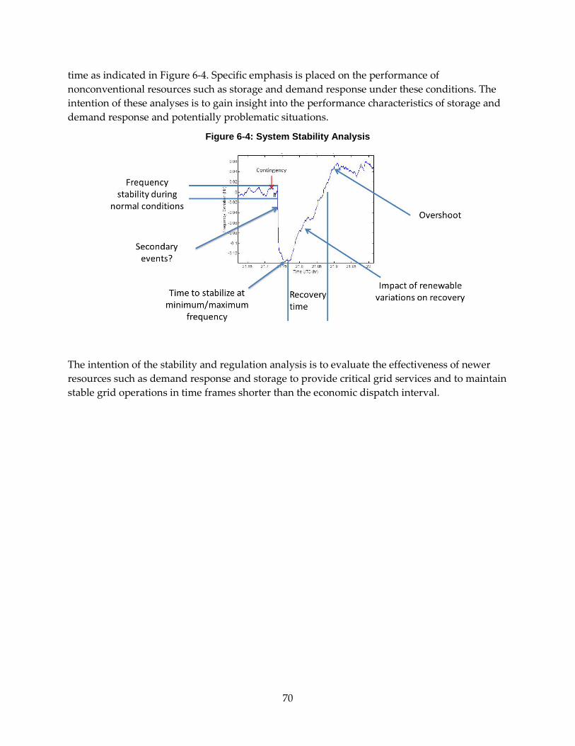
70
time as indicated in Figure 6-4. Specific emphasis is placed on the performance of nonconventional resources such as storage and demand response under these conditions. The intention of these analyses is to gain insight into the performance characteristics of storage and demand response and potentially problematic situations.
Figure 6-4: System Stability Analysis
The intention of the stability and regulation analysis is to evaluate the effectiveness of newer resources such as demand response and storage to provide critical grid services and to maintain stable grid operations in time frames shorter than the economic dispatch interval.

71
CHAPTER 7: Extensions to California ISO High Load Model This chapter explains the data in the production simulation model provided by California ISO and the LLNL modifications that were necessary to support stochastic unit commitment, 5-minute economic dispatch, demand response, energy storage, and other new features. The chapter also describes the cases that were analyzed with the model.
7.1 Description of the WECC Regional Model A model built by California ISO and its contractors to conduct renewable integration studies was modified to perform the analysis in this study. The version of the model developed to analyze the High Load Case was used (Rothleder 2011).
Several major modifications were required. First, the California ISO model performed both day-ahead unit commitment and real-time economic dispatch calculations at hourly intervals. As indicated previously, this study uses the new interleaved mode of PLEXOS to model day-ahead unit commitment at hourly time steps and economic dispatch at 5- minute time steps. This shorter interval for economic dispatch required several modifications to the original California SIO model. Second, this study performs stochastic unit commitment calculations. This added analysis complexity required additional modifications to the model. A summary of the major changes to the model is provided in Table 7-1.
Table 7-1: Changes to the CAISO High Load Model to Enable Five-Minute Dispatch
Change Purpose 1 Switch the Upscaling Method from Step to
Interpolate in the three files passed (in-memory) from day-head (DA) model to real time (RT) model:
Units generating from Day Ahead (DA) UC DA Generation DA Pump Load
Due to the way PLEXOS implements interpolate, changing from step to interpolate delays the RT results one hour with respect to the DA solution. This delay required modifying most of the RT input files to account for the hour shift of the DA files to ensure consistency between the two models.
2 Modify the Commit property for some generators in the RT simulation.
A number of generators were being committed in the DA model, then not being committed in RT model resulting in an undergeneration of the system. The generators were changed to obtain the commitment state from the DA results, and others were removed from the slow start DA designation so the RT could dispatch them if required.
3 New load following (LF) requirements files. The existing LF files did not provide sufficient reserve for meeting the RT changes during certain times of the day and provided too much during other times. The new files are based on the forecast data and projected variations.

72
Change Purpose 4 New formatting for the file “Fixed Outages –
Units Out.csv” The old files were based on an interval that has a different time meaning in the RT and DA models, so the outages were shifted to be actual times. Furthermore, allowing this to happen in RT forced very sudden changes on the system resulting in large price spikes, so the files were modified to mitigate this spike.
5 Create generic generators for every region within California and the out of state (OOS) WECC regions. They are able to provide energy and spinning & non-spinning reserves.
These new generator are very expensive, but the OOS regions were deficient in some ancillary service generation in the 5-minute solutions. These generators provide the system with additional reserve capacity and generation capacity to meet the requirements.
6 Lock down the RT generation to DA generation for units with daily, weekly, or monthly energy limits.
Failure to perform this lockdown created infeasibilities in the RT model.
7 Modify pumped storage units to associate “Fixed Pump Load” to “DA Pump Load” and “Fixed Load” to “DA Generation,” add fixed load penalties, and relax end volume constraints in RT model because the values are fixed.
Failure to perform this lockdown created infeasibilities in the RT model.
8 Remove the Fixed Load property from some generators.
Some generators were fixed in the DA model for unknown reasons.
9 Remove the ability of providing load following from some generators.
A number of generators were providing load following even though they were not physically capable of performing that duty in the RT simulation at five minute intervals.
10 Modify a small number of units so they were available in the RT simulation as well as the DA model.
See Item 2 (Commit property).
11 Add Max Ramp Up and Max Ramp Down properties to transmission lines.
The transmission lines were fluctuating unrealistically in many simulations. Putting ramp limits on them dramatically smoothed the results and the prices.
12 Use an additional Look-ahead of 1 hour. Resulted in improved price stability
13 Switch from Do Not Allow Non-convex Curves to Optimize with Non-convex Curves under the Production Tab.
Eliminated some warnings in PLEXOS, no observed difference in price
14 Use 0.05% Optimality Tolerance in the DA simulation and 0.01% in the RT.
Allowed more precise solutions in RT model. Computational performance was not greatly impacted, as the DA model takes much longer to run than the RT.
15 Use polishing of the Integer programming solution
These heuristics in the CPLEX code improve solution quality and speed.

73
Change Purpose 16 Allow Unserved Energy and Dump Energy
under Nodes Settings. Provides the system with a way to always be feasible.
17 Modify the “Enforced from (kV):” under the Transmission Tab so the transmission constraints are applied.
This change fixed a problem with PLEXOS ignoring transmission limits.
18 Remove MUNI Regional Constraints. These constraints were frequently being violated and seemed redundant given other constraints in the system, so they were removed. All AS requirements were assumed to be met at the California ISO level.
19 Fix Commit = 1 in some Renewable Generation OOS.
Some renewable generators were being dispatched even though they did not have this capability. This change fixed that issue.
20 Add new report properties under the Report fields
Line: Available Transfer Capability Region: Undispatched Capacity Node: Generation
7.2 Modeling Demand Response Demand response is available from a range of residential, commercial, and industrial providers. Each class of providers has different capacities to provide demand response for different grid applications (for example, load following at the 5- minute timescale or regulation at the 4- second timescale) at different times of the day and at different seasons of the year.
Several infrastructure challenges would need to be met before DR could replace conventional regulation capacity on a MW-for-MW basis. First, DR must match the latency of the response that can be achieved with conventional generation. For this study, the team assumed that DR that would be used for regulation would be under direct control by the California ISO with minimal latency. Second, DR must be as reliable as conventional generation. However, to use DR, the system must ensure that the device being controlled is actually on at the time it is to be regulated. This might be ensured through a mechanism to verify availability of the resource, or through a contractual obligation on the part of the DR provider. Finally, DR resources may be subject to demand rebound. For example, if an air-conditioning unit being used for DR receives too many regulation up signals over a short period, the space being cooled would heat up to unacceptable levels. In subsequent periods, the device may not be able to provide additional capacity for regulation up. In practical terms, 1 MW of DR capacity will probably displace less than 1 MW of conventional capacity because the equipment has power supply as a secondary function. This analysis finds an upper bound on the value of DR by assuming that it can replace conventional capacity on a MW-for-MW basis.
7.2.1 Characterization of Demand Response Resources DR is characterized by the power and energy levels available, the speed of response, and, therefore, the applications it can serve, and the rules under which it is dispatched. The Demand

74
Response Research Center (DRRC) provided LLNL with an estimate of the level of power that might be available for each type of service provided. Power levels are provided by type of provider, hour of the day, season, and IOU service area. Data are provided for each of the major utilities in the state:
• Southern California Edison
• Los Angeles Department of Water and Power
• San Diego Gas & Electric Company
• Pacific Gas and Electric – Bay Area
• Pacific Gas and Electric – Valley Area
• Turlock Irrigation District
• Sacramento Municipal Utility District
• Imperial Irrigation District
The data are also characterized in terms of the following classes of providers:
• Residential water heating
• Residential cooling
• Outdoor lighting
• Commercial cooling
• Commercial ventilation
• Commercial lighting
Figure 7-1 shows an example of some of the data provided by the DRRC, partitioned by class of provider. The data in the figure show maximum available capacity of DR for each hour of the day. The capacity associated with each of the six classes of providers and the total capacity available are shown in the figure. Examples and additional descriptions of the data sets provided are included in Appendix C.

75
Figure 7-1: Demand Response Availability by Source and Total in SCE on August 2, 2020
7.2.2 Modeling Demand Response in PLEXOS Each type of provider is energy-limited and can provide the capacity shown in the figure for only one hour. Hence, if all the DR capacity is requested in Hour 16 shown in the figure, 2,000 MW and 2,000 MWh could be provided. If all DR were requested in Hour 4, only 1,000 MW and 1,000 MWh would be available. In PLEXOS, DR was modeled as an energy limited generator with a different capacity in each hour. Two modeling approaches could be used to constrain the available energy: the energy at the peak capacity (2,000 MWh in the example shown) and the energy at the average capacity (1,500 MWh in the example shown). The latter approach was used for the analysis.
In the analysis, three applications for DR were modeled: regulation, load following, and economic. Regulation DR capacity reduces the regulation requirements specified in the PLEXOS model. The PLEXOS input files with these regulation requirements are modified accordingly for DR resources that are dedicated to providing this service. The load following DR capacities are specified as resources available in the PLEXOS short-term model for hourly dispatch in day-ahead markets. The economic DR resources are made available in the PLEXOS real-time model for economic dispatch in 5- minute time steps. Three price tiers of $80/MWh, $105/MWh, and $130/MWh are used to model economic DR. The lowest cost resource is dispatched on 75 PERCENT of the days, the medium cost resource is dispatched about 15 days, and the high price resource is dispatched on a few peak days.

76
7.3 Modeling Storage Several types of storage have been included in the analysis. Some have high capital costs per unit of energy storage and are better suited for small-scale storage (for example, flywheels and batteries) and are best suited for regulation and possibly some load following or peak shaving. Large-scale storage (for example, pumped hydro) is suitable for energy shifting, regulation, and load following.
The characteristics of each of the storage technologies considered are shown in Appendix D. In the production simulation model the team implemented:
• Lithium ion batteries
• Flow batteries
• Compressed air energy storage
• Pumped hydro
These technologies have the following characteristics in the production simulation model:
Table 7-2: Performance and Cost Characteristics of Storage Technologies
Technology Round-Trip
Efficiency
Variable O&M Cost ($/MWh)
Capital Cost per Unit Power
($/kW)
Capital Cost per Unit Energy
($/kWh) Lithium Ion battery (4 hr.)
85% 0.25** 3,600 900
Flow battery 65% 0.25** 1,860 372 Compressed air (5 hr.) 70%* 6 2,000 400 Pumped hydro 60-80% Small Sunk cost Sunk cost
*** Energy ratio (kWh-In/kWh-Out) Compressed air storage system modeled as compressor and generator with heat rate of 3810 BTU/kwh. See Appendix D. ** From PUC data sheet
In the production simulation model used for this analysis, the capacities are given, so the capital costs do not affect operation of the storage. Only the efficiency and operating costs affect the charging and discharging of storage.
Battery and compressed air storage resources are included in the service areas of each of the investor-owned utilities. Pumped hydro storage units are present only in the PG&E valley and SCE service territories.
As noted, the patterns of charging and discharging of storage and related marginal values are determined by the capacities. To explore the space of storage devices, several sets of capacities for discharge power and energy storage capacities are tested.

77
7.4 Cases for Analysis Cases are specified, simulated, and compared to estimate the benefits of adding storage and demand response resources. The common case for comparison is termed the Original model. This corresponds to the California ISO model with modifications as described above. This model includes the economic demand response resources that were provided by California ISO and the file of regulation reserve requirements for each hour of the year. This model is run for all the days in the year.
A second case, which uses the Baseline model, is also executed for all the days in the year. This model includes several small storage devices, regulation capacity equal to original California ISO values minus the demand response capacity specified by the DRRC for regulation, and both the economic (bid and dispatched in the real-time markets) and load following (bid and committed in the day-ahead market) demand response. This baseline model incorporates small amounts of each of the types of resources of interest. Finally, this model is used to identify 24 representative days for more detailed analysis. Clustering methods similar to those described in Chapter 5 are used to select the representative days and weights to apply to them.
Results from these two cases are analyzed to confirm that the production simulation model is producing realistic results. For example, results are examined to confirm that they contain no unrealistic price spikes that indicate model infeasibilities and that the charging and dispatch of storage occur in reasonable patterns in the day-ahead and real-time phases of the production simulation model. Finally, the team confirmed that using demand response, especially the load following demand response, occurs during the most stressful (highest price) periods.
Additional cases are configured to explore other issues, including:
1. Reducing regulation requirements.
Based on Original model, reduce regulation requirements to assess the total system cost reduction resulting from replacing conventional regulation capacity with demand response or storage. To represent demand response, use the regulation demand response capacity specified by DRRC to reduce the conventional regulation capacity requirements that were specified in the original California ISO model.
2. Adding storage power.
Increase the power levels of Li-ion batteries, flow batteries, and CAES to observe the change in operation costs and patterns of operation. Keep the discharge time constant so energy storage capacity increases in proportion to the power level (that is, add MWs of Li-ion battery capacity while maintaining a 4-hour discharge time). Assess the marginal value of adding discharge power and look for market saturation effects.
3. Adding storage energy.
Fix the power levels of Li-ion batteries, flow batteries, and CAES and increase discharge times to observe the change in operation costs and patterns of operation. Assess the

78
marginal value of adding energy storage capacity and identify effective storage system designs.
4. Modifying demand response capacity.
Model a set of demand response capacities added to the Original model to observe the change in operation costs and patterns of operation. Assess the marginal value of both the power and energy capacity offered by demand response program participants. Make several runs with different combinations of power and energy availability. Run the variations on a subset of days that seem to have the largest impact on economic value.
5. Removing economic demand response.
Remove the economic demand response from Original model to observe the change in operations costs and patterns of operations. This is the demand response originally used by California ISO. It simulates demand response that is bid into the market. It specifies a price, power, and energy.
6. Adding load-following demand response.
This demand response is specified as power and energy in Original model. It should be dispatched optimally to use the energy. This identifies the value (price) of energy from demand response.
7. Changing the prices of economic demand response.
Change prices of demand response in Original model to a set of prices that are expected to cause the demand response to be dispatched over the seasons somewhat closely to the specifications for the California ISO demand response product. California ISO allows bid in demand response to be dispatched 15 times for a total of 48 hours each season (winter and summer).

79
CHAPTER 8: Results From Production Simulation Model This chapter chronicles results from the production simulation model before demand response and energy storage resources are added to the system (the Original case). The chapter describes patterns of resource use and prices throughout the year. In effect, the market into which storage and demand response can sell services is characterized here. Results from a second case where small amounts of storage and demand response have been added are also discussed (the Baseline case).
8.1 Commitment and Economic Dispatch Patterns 8.1.1 Original Case Dispatch PLEXOS production simulation models were run for all days of the year for the Original case. Typical generation patterns for five days during the year are shown in Figure 8-1 through Figure 8-5.
Figure 8-1: Generation Pattern for January 15 (Original Case)
Figure 8-1 depicts a winter day. As shown in the blue region on the left side of the figure, wind generators provide power throughout the night but stop generating at 11 a.m. on this winter day. Solar generators provide output during the day but are off by the time the system peak of 45 GW is reached at 7 p.m. This causes the steep ramp up to system peak load. The grey area in the upper right portion of the figure representing storage is mostly hydroelectric pumped storage. This pumped storage helps meet the system peak. Imports, the red area, provide most of the energy to meet the system peak. The day-ahead load forecast (DA curve) and real-time loads (RT curve) are fairly close to one another.

80
Figure 8-2: Generation Pattern for April 28 (Original Case)
On this spring day shown in the figure above, wind generators provide energy throughout the day, although the wind power output during the evening and early morning is significantly greater than during the middle of the day. Hydroelectric power output is steady throughout the 24-hour period due to snowmelt, and power is imported to the State to help meet system peak and at night when prices are low. The 42 GW system peak at 7 p.m. is not significantly higher than the load at noon.
Figure 8-3: Generation Pattern for June 24 (Original Case)
On this day in early summer shown in the figure above, wind generators provide power throughout the day. Peak load of about 52 GW occurs earlier in the day, about 3 p.m., and the 7 p.m. peak is less pronounced than during the spring. There is a significant increase in natural

81
gas generation to meet the system peak. The real-time load (RT) is slightly higher than the day-ahead forecast (DA) used for unit commitment during the system peak.
Figure 8-4: Generation Pattern for August 13 (Original Case)
On this midsummer day shown in the figure above, wind generators provided significant power throughput the day. Hydroelectric and gas generators ramp up to meet the daily peak of 62 GW at about 5 p.m. Solar output is significantly diminished by the time peak load is experienced.
Figure 8-5: Generation Pattern for November 12 (Original Case)
On this fall day shown in the figure above, wind generation is low in the early morning but picks up in the evening. Hydroelectric generation and imports are used to meet the peak at about 7 p.m.

82
8.1.2 Baseline Case Dispatch PLEXOS production simulation models were also run for all days of the year for the Baseline case. This case added the demand response and storage resources to the Original case that are shown in Table 8-1.
Table 8-1: Resources Added for the Baseline Case
Resource Quantity (MW)
Flow battery 100
Li-ion battery (4 hr.) 100
Li-ion battery (15 min) 200
Compressed air (CAES) 100
Battery for regulation 200
Load-following DR File1
Economic DR File2
DR for regulation File3 1 MW capacity of DR available for day-ahead bids for each hour of the year provided by DRRC 2 MW capacity of DR available for economic dispatch provided by DRRC 3 MW capacity of DR available for regulation provided by DRRC
The capacities for each of the four storage technologies were split between the PG&E Bay Area and SCE. The “battery for regulation” was simply a reduction in the regulation requirements for each of the two areas. The three DR resources were specified as described in Appendix C. The capacity was split among the eight areas in the model in proportion to peak loads.
Typical generation patterns for baseline case in the winter and summer are shown in Figure 8-6, and Figure 8-7, respectively. A comparison of these figures with the figures for the original case indicates that dispatch results do not differ significantly between the two cases. This is because the baseline case added only 800 MW of storage to meet a 45 GW load, and the price for demand response was so high that it was not dispatched in significant amounts.

83
Figure 8-6: Generation Pattern for January 15 (Baseline Case)
Figure 8-7: Generation Pattern for August 13 (Baseline Case)
8.2 Prices 8.2.1 Original Case Prices and Revenues California ISO prices for energy, ancillary services, load following, average energy costs, and marginal energy costs were computed for each day of the year. Example results are shown below for five typical days in the year.
Energy prices for California are shown in Figure 8-8, and the range of the load-weighted, day-ahead (DA) market price forecasts is shown as the green band. The range of prices is driven by

84
the range of net load scenarios that were produced by the weather and renewable generator models. The mean of these load-weighted, day-ahead forecasts is shown by the blue line in the graph. The actual prices produced by the 5- minute economic dispatch in the real-time (RT) market for the optimized unit commitment schedule are shown by the red line.
Figure 8-8: Energy Prices for January 15 (Original Case)
The data indicate there are three peak price periods at 7:00 a.m., 7:00 p.m., and 10:00 p.m. Energy storage devices would have the opportunity to cycle three times on this day to exploit these energy price differences. The price differentials would have to be sufficient to compensate for the energy losses incurred when cycling the device. For example, the round trip efficiency of a Li-ion battery is 85 percent. Charging the battery with 1 MWh at $45/MWh at 4:00 a.m. and discharging 0.85 MWh for $120/MWh at 7:00 a.m. would yield an operating profit of 0.85*150 – 45 = $83 per MWh charged. For the second cycle, the operating profit from energy arbitrage would be about 0.85*100 – 55 = $30 per MWh charged. The third cycle would yield roughly $60 per MWh charged. The device would earn $173 per MWh of energy storage capacity for the day. The optimization algorithm used by the PLEXOS software would determine when it is optimal to charge and discharge the device. Other operating profits could be earned by the storage device by providing ancillary services.
The price spike in California at 10 p.m. is uncharacteristic of most power systems. The researchers believe it is related to WECC operations outside California. It appears that on some days the price in the rest of the WECC was low enough to cause several major units to turn off around 10 p.m. This made the energy prices in the rest of the WECC very low but caused prices in California to spike briefly. The algorithm in PLEXOS determined it was less expensive to have most of the WECC operate at a lower cost while increasing prices in California for a short period.

85
Figure 8-9 shows ancillary service prices for January 15. As shown by the data in the figure, significant price spikes for regulation up and spinning reserve occur at several points during the day. Regulation down prices are nonzero late at night, in the early morning, and at noon. Nonspinning reserve prices are zero. An energy storage device that was physically capable of responding to 4- second AGC signals and be cycled some fraction of the 22,000 4-second time intervals per day could earn revenues by providing regulation services. Chemical batteries, which have a limited number of discharge cycles, may not be appropriate for this application18F
19.
Figure 8-9: Ancillary Services Prices January 15 (Original Case)
Figure 8-10 shows load-following requirements. These capacity requirements were provided by California ISO and are described in Rothleder 2011. As indicated in the figure, there is a large requirement for capacity at 4 a.m. and 4 p.m. These requirements are driven primarily by uncertainty in renewable generation during those periods.
19 For example, as indicated in Appendix D, Li-ion batteries may be able to support 100,000 cycles at a 5 percent depth of discharge. If the AGC signal changed sign each 4-second interval, there would be 11,000 cycles per day, and the battery would last less than 10 days. If the AGC signal changed sign every 100 intervals, the battery would last approximately 1,000 days or less than three years.

86
Figure 8-10: Load Following Capacities Required on January 15 (Original Case)
Figure 8-11 shows prices for load following. These prices are the shadow prices19F
20 associated with the load-following constraints in the production simulation model. They estimate the market value of flexible ramping products that California ISO may introduce in the future. Load-following prices on that day follow patterns similar to those of regulation and spinning reserve prices. However, signals for load following occur at 5- minute intervals corresponding to economic dispatch. Energy storage devices could earn roughly $8/MW for charging in the late evening and early morning (load following down). During high load periods, storage devices could earn more than $70 per MW for discharging during peak hours (following load up).
20 Shadow prices, or dual variables, are estimates of the value of relaxing a constraint by one unit. For example, the model requires 500 MW of load following up capacity at 7 a.m. on January 15. The cost of operating the system in that hour could be reduced by $20 if the load following up requirement were reduced to 499 MW in that hour.

87
Figure 8-11: Load Following Prices January 15 (Original Case)
Total hourly costs of operating the grid in California are shown in Figure 8-12. As indicated in the figure, small amounts of ancillary service costs are incurred at several times during the day, while load following costs are only incurred in the early morning and before the evening peak. The costs of carbon emissions contribute significantly to the total. Finally, the “cost to load” is the product of the total load and the marginal price.
Figure 8-12: California Total Hourly Costs on January 15 (Original Case)

88
Costs in the WECC are shown in Figure 8-13. As indicated in the figure, ancillary service costs are incurred throughout the day. Significant transmission congestion charges are incurred.
Figure 8-13: WECC Hourly Total Cost on January 15 (Original Case)
Figure 8-14 shows the energy prices for April 28. The price profile for this spring day has only one peak, which limits the profitability of energy storage. The operating profit for energy arbitrage with a storage device vice that has an 85 percent round trip efficiency would be 0.85*120-40 = $80/MWh of energy storage capacity.

89
Figure 8-14: Energy Prices for April 28 (Original Case)
Figure 8-15 shows ancillary service prices for April 28. Price spikes for regulation up and spinning reserve occur at several points during the day. Unlike the pattern on January 15, regulation up and spinning reserve prices are nonzero during the middle of the day. Regulation down prices are nonzero late at night, in the early morning, and at noon. Nonspinning reserve prices are zero.
Figure 8-15: Ancillary Services Prices April 28 (Original Case)

90
Figure 8-16 shows load following requirements. As indicated in the figure, there is a large spike in the load following down requirement at 9 p.m. This is probably due to a wind ramp up event in conjunction with falling load during that period.
Figure 8-16: Load Following Capacities Required on April 28 (Original Case)
Figure 8-17 show prices for load following. There are only two peak prices for load following up during the day, rather than the three peaks projected for January 15. The price for load following down late at night is significantly higher than the price projected for January 15. Also note the increase in the load following down price at 9 p.m.
Figure 8-17: Load Following Prices April 28 (Original Case)

91
Figure 8-18 displays total hourly costs of operating the grid in California. Note the high ancillary services and load following costs incurred at 3 a.m., and the spike in generation costs at 8 p.m.
Figure 8-18: California Total Hourly Costs on April 28 (Original Case)
Figure 8-19 shows costs in the WECC are shown in. Ancillary service costs are incurred throughout the day, and significant transmission congestion charges are incurred in the early morning and evening.

92
Figure 8-19: WECC Hourly Total Cost on April 28 (Original Case)
Figure 8-20 illustrates energy prices for June 24. As indicated by the green band in the figure, there is a large variation in maximum energy price due to the variation in possible net load scenarios.
Figure 8-20: Energy Prices for June 24 (Original Case)

93
Figure 8-21 shows ancillary service prices for June 24. A price spike for regulation up and spinning reserve occurs 3 p.m. Regulation down prices reach $40/MW late at night, in the early morning. Nonspinning reserve prices are zero.
Figure 8-21: Ancillary Services Prices June 24 (Original Case)

94
Figure 8-22 displays load following quantities. The load following down requirements remain high throughout the day and peak at 9 p.m.
Figure 8-22: Load Following Requirements on June 24 (Original Case)
Prices for load following, which are shown in Figure 8-23, closely follow ancillary service prices.
Figure 8-23: Load Following Prices June 24 (Original Case)
Figure 8-24 shows total hourly costs of operating the grid in California. Ancillary service and load following costs are a small fraction of total costs.

95
Figure 8-24: California Total Hourly Costs on June 24 (Original Case)
Figure 8-25 shows costs in the WECC. Significant ancillary service and load following costs are incurred at 3 p.m.
Figure 8-25: WECC Hourly Total Cost on June 24 (Original Case)

96
Figure 8-26 shows energy prices for August 13. The day-ahead ensemble forecast led to a prediction of high energy prices around 4 p.m. The actual price peak occurred during a short interval about 8 p.m.
Figure 8-26: Energy Prices for August 13 (Original Case)
Figure 8-27 illustrates ancillary service prices for August 13. A price spike for regulation up and spinning reserve occurs around 3 p.m. Nonspinning reserve prices are non-zero at this time.
Figure 8-27: Ancillary Services Prices August 13 (Original Case)
Figure 8-28 shows load following requirements. Load following up requirements peak at noon, while load following down requirements increase steadily throughout the day.

97
Figure 8-28: Load Following Requirements for August 13 (Original Case)
Prices for load following, which are shown in Figure 8-29, closely follow ancillary service prices.
Figure 8-29: Load Following Prices August 13 (Original Case)
Figure 8-30 displays total hourly costs of operating the grid in California. Hourly costs on August 13 are nearly double the costs incurred in April and June.

98
Figure 8-30: California Total Hourly Costs on August 13 (Original Case)
Figure 8-31 shows costs in the WECC. Significant ancillary services and load following costs are incurred at 3 p.m. Emissions costs are significant throughout the day.
Figure 8-31: WECC Hourly Total Costs on August 13 (Original Case)
Figure 8-32 shows energy prices for November 12. As indicated in the figure, one or more net load scenarios in the day-ahead ensemble forecast lead to a wide range of possible prices at 7 p.m. The real-time price pattern indicates that renewable generation was higher than forecast, and the spike in prices was avoided.

99
Figure 8-32: Energy Prices for November 12 (Original Case)
Figure 8-33 shows ancillary service prices for November 12. Regulation up and spinning reserve prices rise from zero at 4 a.m., and a price spike occurs at 3 p.m. Nonspinning reserve prices zero throughout the day.
Figure 8-33: Ancillary Services Prices November 12 (Original Case)
Figure 8-34 illustrates load following requirements. The patterns on this fall day are similar to those observed in the spring.

100
Figure 8-34: Load Following Requirements on November 12 (Original Case)
Prices for load following, which are shown in Figure 8-35, closely follow ancillary service prices.
Figure 8-35: Load Following Prices November 12 (Original Case)
Figure 8-36 shows total hourly costs of operating the grid in California. A large spike in generation costs occurs at 10 a.m.

101
Figure 8-36: California Total Hourly Costs on November 12 (Original Case)

102
Figure 8-37 shows costs in the WECC. A similar spike in generation costs occurs at 10 a.m.
Figure 8-37: WECC Hourly Total Costs on November 12 (Original Case)
Energy prices for the entire year are shown in Figure 8-38, where red spots correspond to high prices per MWh as indicated by the scale on the right. As indicated in the figure, in January there are two periods of high prices at 8:00 a.m. and 8:00 p.m.. The rest of the year, there is only one period of high prices. This occurs at 4:00 p.m. during the summer and at 7:00 p.m. or 8:00 p.m. during the rest of the year. The period of high prices lasts three or four hours during the summer and one or two hours during the rest of the year.
Figure 8-38: Energy Prices by Day and Hour of the Year (Original Case)
$/MWh
Hour
5 10 15 20
Feb
May
Aug
Nov
0
20
40
60
80
100
120

103
Figure 8-39 shows prices for following load up. Two periods of high prices, in the morning and late afternoon, are present throughout the year. Prices are high for several hours per day during July.
Figure 8-39: Load Following Up Prices by Day and Hour of the Year (Original Case)
$/MW g p p
Hour
5 10 15 20
Feb
May
Aug
Nov
0
20
40
60
80
100
120
Figure 8-40 displays prices for following load down. One period of high prices, from about 10:00 p.m. to 5:00 a.m., are present throughout the year. Prices are highest during the spring and early summer, when wind generation levels are highest and most volatile. Note the change in scale to a maximum price of $50/MW. Load following down resources are less valuable than load following up.
Figure 8-40: Load Following Down Prices by Day and Hour of the Year (Original Case)
$/MW g p
Hour
5 10 15 20
Feb
May
Aug
Nov
0
5
10
15
20
25
30
35
40
45
50

104
Figure 8-41 shows regulation up prices are shown in. Price patterns are very similar to the prices observed for load following up.
Figure 8-41: Regulation Up Prices by Day and Hour of the Year (Original Case)
$/MW g p
Hour
5 10 15 20
Feb
May
Aug
Nov
0
20
40
60
80
100
120
Figure 8-42 shows regulation down prices. Price patterns are very similar to the prices observed for load following down.
Figure 8-42: Regulation Down Prices by Day and Hour of the Year (Original Case)
$/MW
Hour
5 10 15 20
Feb
May
Aug
Nov
0
5
10
15
20
25
30
35
40
45
50
Figure 8-43 displays spinning reserve prices. The same general pattern of high prices during the morning and evening peaks can be observed. However, there are random times during the year when high prices are present.

105
Figure 8-43: Spinning Reserve Prices by Day and Hour of the Year (Original Case)
$/MW p
Hour
5 10 15 20
Feb
May
Aug
Nov
0
20
40
60
80
100
120
Figure 8-44 shows nonspinning reserve prices. Prices are non-zero only during peak hours in July when the system experiences maximum loads for the year.
Figure 8-44: Nonspinning Reserve Prices by Day and Hour of the Year (Original Case)
$/MW p
Hour
5 10 15 20
Feb
May
Aug
Nov
0
20
40
60
80
100
120
Figure 8-45 shows total revenues for energy and each ancillary service. As indicated by the data in the figure, load following up (LFU), regulation up (RegU), and spinning reserve (Spin) provide potential revenue streams that are about 20 percent of the revenues from energy sales. Load following down (LFD) and regulation down (RegD) revenue streams are significantly smaller than the other sources. Current California ISO regulations require the ability for full power output for 30 minutes to qualify as spinning reserve. Battery systems that can provide full power for only 15 minutes must be de-rated by a factor of two.

106
Figure 8-45: Annual Revenues from Energy and Ancillary Services (Original Case)
8.2.2 Baseline Case Prices and Revenues California ISO prices for energy, ancillary services, load following, average energy costs, and marginal energy costs were computed for the baseline case for each day of the year. Example results are shown below for January 15 and June 24.
Figure 8-46 shows energy prices for January 15. Price patterns do not vary significantly from the Original case.
Figure 8-46: Energy Prices for January 15 (Baseline Case)
Figure 8-47 shows ancillary service prices for January 15. Prices do not vary significantly from those estimated for the Original case.

107
Figure 8-47: Ancillary Services Prices January 15 (Baseline Case)
Prices for load following, which are shown in Figure 8-48, closely follow ancillary service prices.
Figure 8-48: Load Following Prices January 15 (Baseline Case)
Figure 8-49 shows total hourly costs of operating the grid in California. A comparison with the costs in the Original case shows that this addition of a small amount of storage and demand response has eliminated most of the load following costs that were incurred at 5 a.m. In addition, a large spike in imports at 10 p.m. has been eliminated.

108
Figure 8-49: California Total Hourly Costs on January 15 (Baseline Case)
Figure 8-50 illustrates costs in the WECC. Load following costs at 5 a.m. have been reduced due to the addition of the storage and demand response resources specified for the Baseline case. Other cost patterns are similar to those realized in the Original case.
Figure 8-50: WECC Hourly Total Costs on January 15 (Baseline Case)
Figure 8-51 shows energy prices for June 24. Price patterns do not vary significantly from the Original case.

109
Figure 8-51: Energy Prices for June 24 (Baseline Case)
Figure 8-52 shows ancillary service prices for June 24. Prices are similar to those estimated for the Original case.
Figure 8-52: Ancillary Services Prices June 24 (Baseline Case)
Prices for load following, which are shown in Figure 8-53, closely follow ancillary service prices.

110
Figure 8-53: Load Following Prices June 24 (Baseline Case)
Figure 8-54 shows the total hourly costs of operating the grid in California. The generation cost spike present in the Original case is not present in the Baseline case. The 600 MW of storage and the demand response resources may have been sufficient to eliminate the cost spike.
Figure 8-54: California Total Hourly Costs on June 24 (Baseline Case)
Figure 8-55 shows costs in the WECC. The cost spike present in the Original case is not present in the Baseline case.

111
Figure 8-55: WECC Hourly Total Costs on June 24 (Baseline Case)
8.3 Clustering Days Although all the days in the year were analyzed for these two cases, the example results shown above reflect results from a randomly selected day for each season. These four days may not be very representative of the year. It would be advantageous to identify a small number of days that best represent the behavior of the system for the year. Analysis of this representative set of days would allow more cases to be run for a given amount of computational resources.
As discussed and illustrated in Chapter 5, statistical clustering methods can be used to select a subset of objects that best represent the entire population. In that analysis, the K-means clustering method was used to select representative members from an ensemble of 30 net load trajectories. The daily peak load and maximum ramp rate were used as key features to cluster the net load trajectories.
Here a similar technique was used to select representative days for the year. Hourly system marginal prices, hourly loads, and the daily ratio of peak to average price were used as the features in the clustering algorithm. Figure 8-56 shows one example cluster, which plots system marginal prices verses hour of the day.

112
Figure 8-56: One Day Representing a Cluster
As indicated in the figure, the clustering algorithm has identified 54 days with marginal prices similar to those realized on November 12, 2020 (the thick red line in the figure). Hence, November 12 is selected as one of the representative days with weight 54/365. The other representative days selected are shown in Table 8-2.
0 5 10 15 20 2530
40
50
60
70
80
90
100
110cluster 15, 2020-11-12
Normalized Power
Hour in day

113
Table 8-2: Clusters With Representative Days and Number of Members
Representative date
Days in cluster
Description
1/15/2020 49 winter 2/9/2020 36 winter weekend 4/11/2020 11 spring weekend 4/28/2020 55 spring 5/21/2020 26 Late spring 5/31/2020 1 high renewable day 6/13/2020 11 early summer weekend 6/24/2020 15 early summer 7/5/2020 17 Summer Weekend 1 7/15/2020 1 High Load day 7/16/2020 1 High Load day 7/19/2020 6 Summer Weekend 2 7/21/2020 2 Summer Cluster 1 7/22/2020 2 Summer Cluster 2 7/23/2020 2 Summer Cluster 3 7/24/2020 3 Summer Cluster 4 7/31/2020 1 high load day 8/2/2020 6 Summer Weekend 3 8/13/2020 19 summer 9/8/2020 12 Late Summer 1 9/24/2020 7 Late Summer 2 9/30/2020 4 early fall 11/12/2020 54 fall 11/21/2020 21 fall weekend
This careful selection of representative days and associated weighting closely approximates the behavior of the system over the full year. Figure 8-57 shows a comparison of prices for all hours of the year. As indicated by the two price duration curves, the range of prices for the selected days closely approximates the range of prices for the entire year.

114
Figure 8-57: Comparison of Prices on Cluster Days With Prices for Full Year

115
CHAPTER 9: Value of DR and Storage for Regulation This study evaluates the effectiveness of DR and storage in providing regulation from both an economic and an engineering point of view. The economic evaluation is addressed in this chapter. It assesses the operating cost savings that could result from substituting DR and storage for the regulation capacity provided through conventional generation. Chapter 11 describes analysis with a system regulation and stability model to evaluate the ability of DR and storage to operate under circumstances and maintain stable behavior when the system is perturbed.
When demand response and storage replace part of the conventional generation reserved for regulation services, this conventional generation capacity can be used to provide energy, or it can be shut down if it is not needed for energy. This has the effect of both reducing the operating cost of the system and of reducing the market price for regulation services. This section assesses the reduction in costs that could result from using DR or storage in place of conventional generation for regulation.
9.1 Cost Reductions From DR for Regulation The primary regulation expense to the system operator is the cost of procuring the regulation capacity either in the day-ahead market or, occasionally, in the real-time market. The model includes a California ISO-specified level of regulation resources each hour. The model solution ensures that the specified level of capacity is available and running each hour.
However, the model does not explicitly model the operation of the regulation resources. It dispatches the system on 5-minute time steps, while regulation refers to adjustments of power on the sub 5-minute time steps. In actual operation, the regulation capacity is dispatched above and below the capacity level that is specified each hour. The average operation cost is generally about equal to the average cost of operating the level of capacity that is procured. The model provides a close estimate of the cost of procuring and operating the conventional regulation resources.
9.1.1 Total Cost Reductions With DR The team assessed an upper bound on the value of DR by assuming that DR can replace conventional capacity for regulation on a MW-for-MW basis. The model was run twice to make the assessment. The first run included the same hourly requirements for regulation capacity as were assumed in the Original case, which is described in Chapter 7. The second run assumed that DR can reduce this requirement. Accordingly, the regulation capacity requirement was reduced by the full amount of regulation capacity specified by the DRRC. The difference between these runs provides an upper bound on the benefit that would be provided by substituting DR for conventional regulation.
The effect of reducing the requirement for conventional regulation capacity can be measured either by the change in the total annual operating cost of the system or by the change in the cost

116
of procuring conventional regulation resources. The first measure assesses the actual overall savings that will result from the reliance on DR. These benefits will accrue to both ratepayers and generators. The second measure assesses the change in the cost of procuring conventional regulation resources by the system operator. The model solution estimates the price that would prevail in the ancillary services market for regulation up and regulation down services. The cost of procuring services is estimated as the total capacity required times the market price for the service. The analysis is based on clusters of days that represent the days of the year, as described in Chapter 8.
In either case, the analysis estimates only the reduction in cost due to reliance on DR. It does not include the cost of procuring DR (for example, the cost of communication and control infrastructure and the cost of contracts to provide DR). This provides an estimate of the maximum value of DR and the maximum amount that the system operator should be willing to pay for the DR services. The analysis was based on clusters of days that represent the days of the year, which is described in Chapter 8. Results are shown in Table 9-1.
Table 9-1: Annual System Costs for California at Different DR Capacities for Regulation
Case
Operating cost
($M/yr.)
Conventional reg up procurement
cost ($M/yr.)
Conventional reg down procurement
cost ($M/yr.) System with no demand response resources
11,409 84 26
Demand response resources provide part of regulation requirements
11,378 55
16
Difference 31 29 10
As indicated by the table data, introduction of DR resources to provide regulation reduces operating costs by $31 million per year. This difference is only 0.3 percent of the total annual operating costs. The costs of procuring regulation up and down services are reduced by $39 million per year.
9.1.2 Sources of Costs Savings With DR The reduction in cost of procuring regulation up and regulation down services is partly due to the reduction in the total amount that must be procured using conventional generation, and the “quantity effect,” and partly due to the fact that the price (equivalent to the marginal cost) of providing regulation services is decreased when DR provides part of the capacity, the “price effect.” By examining the changes in quantities and prices, the magnitude of both effects can be estimated.
The quantity effect is roughly equal to the change in total quantity of regulation services demanded from the conventional generators, multiplied by the price. Here the price is the set of prices that prevail when all of the regulation is provided from conventional generators.
Table 9-2 shows the average price of regulation services for the Original case (without DR) and the change in the average capacity of regulation services required each hour. In general, this

117
approach will somewhat overestimate the impact of the change because it is based on the effect of the first increments of change, and later increments will have smaller effects.
Table 9-2: Costs Due to Change in Regulation Capacity From Conventional Generation
Regulation
service
Average price of regulation
($/MW per hr.)
Change in average regulation required from conventional generators
(MW per hour)
Total annual savings due to
reduction in quantity ($M/yr.)
Regulation Up 13.8 130 15.7 Regulation Down 4.6 91 3.7
The first column of data in the table shows the average price of regulation service (up or down) for the Original case. The second column shows the change in the average MW of regulation required from conventional generation each hour – the change in quantity. The last column is the total annual savings, which is the product of the first two columns and the number of hours in a year (8,760).
The price effect is caused by the reduction in regulation prices resulting from the reduction in capacity required from conventional generators. This is computed as shown in Table 9-3.
Table 9-3: Approximate Change in System Costs Due to the Change in DR Prices
Regulation
service
Change in the average price of
regulation ($/MW per hour)
Average regulation capacity
(MW per hr.)
Total annual savings due
to reduction in price ($M/yr.)
Regulation up 13.72 – 10.50 = 3.22 687 19.4 Regulation down 4.61 – 3.31 = 1.30 693 7.89
The first column shows the computation of the change in the average price of regulation from conventional generators in each hour. The second column shows the average capacity of regulation service (up or down) in the Original case. The third column shows the total annual savings due to the reduction in price (change in average price x average hourly capacity x 8,760 hours per year). This is the change in the cost of regulation capacity if the quantity did not change, but the prices changed.
The estimates of the price effect and quantity effect resulting from the reduction in regulation up capacity shown in the last two tables sum to $35 million per year. This sum is comparable to the change in the cost of procuring regulation up of $29 million per year shown in the first table. These results indicate that the price effect and the quantity effect have similar magnitude, although the price effect is somewhat larger. As noted above, the methods used tend to overestimate the effects, so it is expected that the estimate will be larger than the measured effect.

118
9.2 Cost Reductions of Storage for Regulation Storage could also provide regulation services. This section evaluates the economic impact of using storage to displace conventional generation. Chapter 11 evaluates the effectiveness of storage in providing regulation to maintain system stability.
There are two considerations on the use of storage for regulation. First, because storage is energy-limited, it can provide regulation up only if it has sufficient energy in storage and it can only provide regulation down if the storage device is only partly charged. A generator is only allowed to offer regulation services if it can guarantee that it will provide the service for a specific length of time. Because regulation requirements are specified in the model on an hourly basis, researchers assumed that a supplier in the market would have to guarantee the ability to provide regulation for at least a full hour. This would require some initial level of energy in storage at the start of the hour and, therefore, a minimum energy capacity of the storage device. The storage can be expected to charge and discharge while it is providing regulation up and regulation down, so the initial energy does not have to be equal to the total energy discharged over the hour. This pattern of charging and discharging occurs on a sub-5- minute basis. However, the production simulation model models dispatch only on a 5- minute basis, so it is not able to determine the charging and discharging of the storage used for regulation and cannot determine the initial stored energy required.
The second consideration concerns the life of the storage device. The device must be capable of charging or discharging in response to signals every 4 seconds. Rapid charge–discharge cycles may limit the life of chemical batteries20F
21 but would have no effect on flywheels.
In the analysis both issues were addressed using optimistic assumptions about the capability of storage. These provide an upper bound on the economic values of storage for regulation. The analysis assumes that the energy capacity of the storage has been sized appropriately to provide regulation services for the required period. It is also assumed that 1 MW of storage discharge capacity can displace 1 MW of up regulation from conventional sources21F
22.
The team focused on the economic value of the power of the storage device. The economic value of storage for regulation is evaluated using the same general approach as was used to evaluate DR: The regulation requirement is reduced from the base case level to assess the reduction in
21 For example, there are nearly 22,000 4- second intervals in a day. If each successive regulation signal changed sign, there would be 11,000 small cycles in a day. As described in Appendix D, a Li-ion battery could provide up to 100,000 cycles at a 5 percent depth of discharge. Such a battery would last only nine days if it were cycled by 5 percent 11,000 times per day. Because of autocorrelation in regulation signals, the number of charge-discharge cycles is likely to be far fewer than 11,000 per day. In addition, extremely shallow discharge cycles may have minimal impact on battery life.
22 A recent study (Kema 2010) indicates that 1 MW of storage could substitute for 2 MW of combustion turbine capacity. This is due primarily to the faster response time of storage (10 MW/sec verses 0.44 MW for a 100 MW storage device or combustion turbine). This substitutability is discussed further in Chapter 11.

119
overall operation cost of the system. Because storage can be available at a constant power level during the full day, it is modeled as a constant reduction in regulation requirement over the day rather than a reduction that varies over the day as was done with DR. This was evaluated using the clusters of days defined previously.
Results are shown in Table 9-4. Similar to the demand response analysis discussed above, the data in the first row assume that all regulation requirements are met with conventional resources. The data in the second row assume that 200 MW of storage capacity will be used to meet regulation capacity requirements.
Table 9-4: Systems Costs at Different Levels of Energy Storage Capacity for Regulation
Operating
cost ($M/yr.)
Cost of procuring conventional regulation up
($M/yr.)
Cost of procuring conventional
regulation down ($M/yr.)
System with no storage resources for regulation
11,409 84 26
System with 200 MW storage resources for reg Up and 200 MW for reg down
11,339 53 13
Difference 70 31 13
The first column of data in the table shows the annual system operating cost for California. The second column of data shows the annual cost of procuring conventional regulation up resources. The last column shows the annual cost of procuring regulation down resources.
As indicated in the last row of the table, the overall system operating cost is reduced by around $76 million per year. The costs are reduced by freeing some generation to provide energy, which allows the system to operate a little more efficiently. The costs of procuring regulation up and regulation down capacity are reduced by about $31 million per year and $13 million per year, respectively. These values are the change in the cost of procuring the regulation services not the cost of providing the service – the procurement costs are determined by the price of the service each hour, multiplied by the capacity required. Similar to the cost benefits of DR, these reflect both a reduction in the quantity of regulation services that must be acquired from conventional generators, and the reduction in the price of regulation services.
Flywheel energy storage devices would be capable of withstanding the constant cycling that regulation services would require. Unlike chemical batteries, flywheels performance does not significantly degrade with charge-discharge cycles.
As indicated in Appendix D, capital costs of flywheels with a 15-minute discharge time are $1.9 million per MW of capacity, and the plant life is 25 years. At a discount rate of 15 percent22F
23, the 23 A recent report (APPA 2012) cites aftertax returns on equity for merchant generators in the PJM Interconnection ranging from 15 percent to 23 percent. Assuming a 20 percent aftertax return on equity, a 10 percent tax rate, an 8 percent corporate bond yield, and 50 percent financing, the pretax weighted average cost of capital is 0.5*20/(1-0.1) + 0.5*8 = 15%

120
levelized cost of operating a flywheel is $294,000 per year per MW of capacity. The 200 MW of flywheel energy storage would cost $60 million per year. Because operating cost savings are $70 million per year, flywheels for regulation may be a viable investment.

121
CHAPTER 10: Demand Response and Storage for Load Following and Energy Arbitrage As discussed in the earlier chapters, a system with 33 percent renewable generation is subject to strong ramps at certain times of the year, most notably in the winter and spring months. The conventional generation must ramp up quickly to compensate for the loss of solar generation in the late afternoon, while load is rising to the daily peak. At other times, there can be sharp net load ramps, both up and down, due to sudden changes in wind power. It is expected that DR and storage could be used to assist the system with load following to meet these ramps.
In addition, demand response and storage can be used to effectively shift load from the peak to off-peak hours. Such leveling of the load would reduce overall system costs. For example, air-conditioning units providing DR could pre-chill buildings before peak demand periods and then shut down during peak demand. Similarly, storage devices could buy energy to charge the device during off-peak hours when energy prices are low, then discharge energy during peak demand when energy prices are high. This process is known as energy arbitrage.
This chapter describes the value that demand response and energy storage provide for load following and energy arbitrage functions.
10.1 Load Following Requirements In a previous study (Rothleder 2011), load following requirements were based upon a statistical (ARMA) model of weather patterns during each season. The variance in the statistical model determined how much load following capacity (MW per minute ramp rate) should be available each hour of the year to accommodate unanticipated changes in net load. The requirements were set to meet the 95th percentile in the distribution of possible ramp rates that the system would need, given the uncertainty in the weather and renewable generation. These hourly requirements for load following were reflected as constraints in the production simulation model.
In this study, load following requirements were established using the statistical properties of the daily net load ensembles described previously in this report. For each hour of each day, a normal distribution was fit to the 30 samples of possible net loads for that hour. The 95th percentile of the distribution of possible ramp rates was computed and used as a constraint in the production simulation model.
10.2 Scenarios for Analysis of DR In the production simulation model, DR is modeled as a generator with a specified maximum power level and a total of available energy over the day. The maximum power level varies from hour to hour in accordance with the power levels described in Appendix B. As discussed in the appendix, economic DR is committed and dispatched according to a fixed schedule in the day-ahead market, while load following DR is dispatched in the real-time market.

122
The total energy that would be available from DR depends on the market rules in place in 2020 and the willingness of DR providers to be curtailed. This analysis established a baseline energy level and then ran a series of cases above and below that level of energy to test the sensitivity of the results. The baseline energy level was obtained by first summing the hourly power levels over each day. This sum would equal numerically the maximum possible energy that could be available if the DR providers were fully dispatched every hour. This quantity was divided by 24 on the assumption that, in fact, each provider would supply energy for only one hour per day. In the analysis, cases were run at this energy level and at 2.0 and 0.5 times this level.
Because the model is an optimizing model, it commits and dispatches economic DR in the day-ahead market according to a fixed schedule and dispatches flexible DR in the real-time market over the day at the hours with the highest system prices. This achieves the greatest reduction in total system costs.
The research team made several runs to assess the value of DR for load following. A full-year run was made using the levels of load following DR power specified by the DRRC. In addition, several runs were made on the clustered days to evaluate the value of the DR at smaller levels than those specified by the DRRC.
The reduction in annual system operating costs for DR used for load following are shown in Table 10-1. The data show the change in operating costs for plants in California, including the costs of importing energy from the rest of WECC.
Table 10-1: System Cost Savings With Demand Response for Load Following
DR configuration Cost ($M/yr.)
Reduction with DR ($M/yr.)
% reduction
No demand response 11,409 DR - vary energy 2 x Baseline energy 11,317 92 0.8% Baseline energy from DRRC 11,325 84 0.7% 0.5 X Baseline energy 11,368 41 0.4% DR Vary power 0.5 X Baseline power 11,365 44 0.4%
As indicated in the table, DR providing load following services can reduce system costs by up to 0.8 percent. These savings are due in part to price spikes in that occur on days with high renewables that could be addressed by a small capacity of DR. As discussed, these estimates assume that the communication and control infrastructure is in place to use the DR on these short timescales and that consumer behaviors will be compatible with such high-frequency variations in demand. Other rows in the table show savings that can be achieved when the power and energy are varied relative to the baseline DR profiles provided by the DRRC. As indicated by the data in the table, if the energy available is reduced by half, the savings are decreased by about half. If the energy available is doubled, the savings increase by only about 10 percent. Hence, there is a market saturation effect at the baseline energy specified by DRRC. If the power is reduced by half, the savings are reduced by about half. These small savings

123
estimates are difficult to measure due to the resolution of the models and tolerances in the solution process.
10.3 Scenarios for Analysis of Storage Load following requirements can raise prices on the system by requiring the dispatch of fast-ramping generators with high operating costs. Storage technologies are generally able to ramp quickly and could meet the need for load following. If they are able to charge when energy costs are low, they may be able to provide load following at a lower operating cost. This analysis assesses the economic value of using storage to meet load following requirements and assesses whether the economic value of load following and energy arbitrage can exceed the capital costs.
10.3.1 Operation of Energy Storage Figure 10-1 shows annual and hourly usage patterns for 50 MW of 4-hour Li-ion battery in the SCE service territory. The figure shows the generation from the battery, where negative generation corresponds to charging. As indicated by the patterns in the figure, usually there are two charge-discharge cycles in the winter, spring, and fall. Charging (dark blue areas) tends to occur between midnight and 5:00 a.m. In the winter, spring, and fall, the system discharges during the morning peak from 6:00 a.m. to 10:00 a.m. The system charges again in the afternoon, then discharges during the evening peak.
Figure 10-1: Generation and Charging for 50 MW of 4 Hour Li-Ion Battery
During the summer, the system cycles only once per day. The charge is maintained through the morning and early afternoon, and the system discharges during the system peak from 5:00 p.m. to 9:00 p.m.

124
Figure 10-2 is a similar diagram depicting the charge state of the 200 MWh of storage capacity. As indicated by the red areas on the right-hand side of the figure, the system is usually fully discharged until about midnight. Charging occurs in the early morning. The horizontal orange lines in the morning indicate that on some days the system will not fully charge by the morning peak.
Figure 10-2: Charge State for 50 MW of 4 Hour Li-Ion Battery in SCE Service Territory MWh
10.3.2 Total Net Revenue and Marginal Value of Storage A storage system can be analyzed from two points of view. First, one can determine whether a given installation will earn a net positive return on investments. However, even if an installation does earn a positive return, it may not be optimally designed for the patterns of load and prices. To evaluate the design of a system, a second approach is used to evaluate the “marginal” values of each component of the system—the charge capacity, discharge capacity, and energy capacity. The marginal value of a system component is the additional value that would accrue to the system if a small increment of capacity were added. For example, the team can assess the additional value of adding one more MWh of energy storage capacity to the system. Because the cost of adding each type of capacity is known, the cost to the value can be compared. If the value is greater than the cost, then it will be best to add more capacity of that type. Analyzing the marginal values of different components allows the authors to better understand how energy storage systems should best be configured for a given set of conditions.
The researchers can assess the net economic value of a given storage installation, specifying the charging and discharging power and energy storage. The net annual revenue can be assessed over a year’s operation as the total value of discharges minus the total cost of charging (accounting for efficiencies and operating costs). To assess the economic viability of the installation, the net annual revenue must be compared to the fixed annual costs and the annualized capital costs of the installation. If the net annual revenue cannot cover the annual costs, then the installation is not economically viable.

125
The total net annual revenue approach assumes that the operation will be the same over the entire life of the installation. A more complete assessment based on net present values of cash flows assesses the stream of capital costs, revenues, and expenditures over the life of the project. This form of analysis can take into account assumptions about changing costs of charging or values of discharging over the life of the project.
10.4 Results for Energy Storage for Load Following and Energy Arbitrage
10.4.1 Cases Analyzed A series of cases were run with the production simulation model to investigate the reduction in value of storage for load following and energy arbitrage as more capacity is added. Power was varied, while energy storage capacity per MW was maintained at a constant level (for example, 4 hours of storage at rated MW power). Large Li-ion, flow battery, and CAES units with 4 hours of run time and small Li-ion units with 15 minutes of run time were analyzed. Descriptions of the cases are shown in Table 10-2.
Table 10-2: Sequence of Runs That Varied Charge/Discharge Power
Power per large storage
unit (MW)
Energy per large
storage unit (MWh)
Power per small
storage unit (MW)
Energy per small
storage unit (MWh)
Full year or
clustered days
Storage5MW 5 20 100 25 clusters Storage10MW 10 40 100 25 clusters Storage30MW 30 120 100 25 clusters Storage100MW 100 400 100 25 clusters Storage300MW 300 1200 100 25 clusters Storage600MW 600 2400 100 25 clusters Storage1200MW 1200 4800 100 25 clusters
Storage technologies were in the PG&E Bay and the SCE regions. This gives a good understanding of the value of storage because storage operation and value is primarily dependent on system prices, and the prices are uniform over these regions. Table 10-3 shows the regional distribution of capacity.

126
Table 10-3: Storage Technology Regions and Capacities
Region Technology Charge/
Discharge Capacity (MW)
Energy Capacity
(MWh) PG&E BAY CAES 5 20 PG&E BAY Flow 5 20 PG&E BAY Li-ion 5 20 PG&E BAY Li-Ion 100 25 SCE CAES 5 20 SCE Flow 5 20 SCE Li-Ion 5 20 SCE Li-Ion 100 25
The model represents dispatching decisions both day-ahead (DA) and during the operating day (real time, or RT). In the model, large storage is scheduled in the DA analysis. This schedule considers the uncertainties in renewable generation and loads in the DA analysis. When modeling the RT, the model charges and discharges the large storage according to this schedule. Small storage is modeled in the RT analysis. The small storage is charged and discharged according to the conditions that were actually realized during the operating day. Within the model, the small storage operation is optimized using perfect foresight over the day. As such, it represents an upper bound on the economic benefits from the small storage.
10.4.2 Economic Dispatch of Storage Operations The figures below illustrate the operation of storage in the model. Storage capacity for three technologies (4-hour Li-ion, flow battery, and CAES) was added the PG&E Valley and SCE service territories. Several runs were made with increasing levels of storage capacity. In the final run, each of the three technologies had 1,200 MW of capacity in each of the two service territories, for a total of 7,200 MW. Figure 10-3 shows conventional generation and storage usage for January 15.

127
Figure 10-3: Usage of 7,200 MW of Storage on January 15, 2020
As indicated by the data in the figure, storage is charged in the early morning when wind energy is available. The storage is discharged during the ramp up to meet the midday peak. Storage is used more heavily to meet the daily peak at 7:00 p.m. A comparison with the generation patterns without storage for this date shown in Figure 8-1 indicates that some imports are being used to charge storage in the middle of the day so that the batteries can replace some imports during the evening peak. The reduction of coal generation at 5:00 a.m. and 7:00 p.m. reflects reductions in coal imports into California from the rest of WECC, not necessarily to cycling of coal plants during these hours.
Figure 10-4 shows energy prices and CAES operation for this same day. As indicated in the figure, there is a rather rapid ramp in the morning, which causes a peak in prices in the morning. Prices also peak in the evening when load peaks. The CAES storage is used to serve both peaks. It recharges somewhat during the midday when prices moderate. The fact CAES discharges to help generate during the morning ramp and then recharges in midday suggests that the high efficiency on discharging makes it worthwhile to discharge in the morning, even though the price differential is not large.

128
Figure 10-4: CAES Operation and Energy Prices on January 15, 2020
Figure 10-5 shows energy prices and Li-ion battery operation for this same day. As indicated in the figure, the Li-Ion battery is used principally to serve the evening peak. This new storage capacity significantly augments the pumped storage that was used in the Original case.
Figure 10-5: Li-Ion Operation and Energy Prices on January 15, 2020
Figure 10-6 illustrates storage usage for June 24. On this summer day, load is about 7 GW larger than the load on January 15. In addition, there is a single peak at 3:00 p.m., rather than the two peaks observed on January 15. Storage resources help level generation from gas between 9:00 a.m. and 7:00 p.m. A comparison with the generation patterns without storage for this date shown in Figure 8-3 indicates that some imports are being used to charge storage in the early morning so that the batteries can replace some imports during the midday peak.

129
Figure 10-6: Usage of 7,200 MW of Storage on June 24, 2020
Energy prices and energy storage operation for this same day are shown in Figure 10-7 and 10-8. Both storage technologies behave similarly on this day, charging early in the morning when there is more wind and imported energy available and discharging during the peak price hours in the afternoon.
Figure 10-7: CAES Operation and Energy Prices on June 24, 2020

130
Figure 10-8: Li-Ion Operation and Energy Prices on June 24, 2020
10.4.3 Value of Storage For each case analyzed, the net revenues (revenues from discharge less costs of charging) to storage have been computed. Net revenues measure the operating profit that a storage owner would receive. These can be compared to the capital costs of the installation to estimate the economic viability of storage investments. Net revenues also measure the net economic benefits that the storage provides to the system. They measure the cost to the system of taking energy out when storage charges and measure the value that the storage provides when it discharges energy back to the system.
The analysis determines the net operating profit for each technology at each capacity modeled. Researchers can then estimate the change in profit as either the power or the energy storage capacity is varied. This is the marginal value of adding either power or energy storage capacity. The marginal value of capacity can be used to determine the incremental value from adding more units of capacity. For an optimized system, capacity should be economically added as long as the marginal value of capacity is greater than the marginal cost. The marginal values of capacity can be estimated from the slopes of the curves of net revenue.
Two parametric studies were conducted. In the first study, the power of the storage devices was increased while holding the discharge time constant. (The energy capacity increases in direct proportion to the power.) In the second study, the power was held constant at 50 MW, while the discharge time was increased. For these runs, three storage technologies were present in two service territories, so the total storage power was 300 MW.
Figure 10-9 shows results of the first study varying power in the PG&E Bay region. The figure shows the annual net revenue for each of the three storage technologies as capacity of each is increased. The curve for the flow battery terminates at a power of 300 MW because it is not dispatched when more storage capacity is available. At the 600 MW point, the 1,200 MW of

131
capacity from CAES and Li-ion batteries is dispatched instead of the 600 MW of flow battery capacity. This is due primarily to the lower efficiency of the flow battery.
The net revenue curves also show a market saturation effect, where each additional increment of capacity is worth less. The knee in the curve at 300 MW and the reduced benefits of additional capacity suggest a goal of 1,800 MW of storage capacity for the State (300 MW x 3 technologies x 2 service territories).
Figure 10-9: Annual Net Revenue of Storage Power in PG&E (4-Hour Discharge Time)
The slopes of the net revenue curves above are plotted in Figure 10-10. This is the marginal value of adding additional storage power. As indicated in the figure, if 1 MW of each storage technology is added to the system, the value of this first MW of CAES is almost $70,000 per year. The values of the first MWs of Li-ion and flow batteries are $45,000/year and $20,000/year, respectively. If the annualized capital costs, annual fixed O&M costs, and variable operating costs are less than these net revenue estimates, the project is economical to build based upon profits from energy arbitrage alone. If costs are higher, other sources of revenues such as ancillary services will be needed to justify the investment.

132
Figure 10-10: Marginal Value of Storage Power in PG&E (4-Hour Discharge Time)
Figure 10-11 shows net revenue curves for SCE. They are roughly 10 percent higher than the PG&E values. The knee in the curves at 300 MW per technology is also present in the SCE data.
Figure 10-11: Annual Net Revenue of Storage Power in SCE (4-Hour Discharge Time)
Figure 10-12 shows marginal value curves for SCE. They are similar to the curves for storage facilities in PG&E’s service territory.

133
Figure 10-12: Marginal Value of Storage Power in SCE (4-Hour Discharge Time)
As indicated, the second study varied the energy storage capacity while keeping power constant at 50 MW per technology per service territory (300 MW total). Figure 10-13 shows results for storage in the PG&E service territory. As indicated in the figure, there is a saturation effect at a discharge time of 3 hours. Storage technologies with discharge times greater than 3 hours are significantly less valuable.
Figure 10-13: Annual Net Revenues of 50 MW Storage Units in PG&E
The marginal values of additional discharge time (or stored energy per unit of power) were computed by taking the slopes of the lines in the curves above. Figure 10-14 shows the results. As indicated in the figure, first MWh of energy storage capacity is worth $1.35 million/year, $800,000/year, and $500,000/year for CAES, Li-ion, and flow batteries, respectively. These

134
revenues are from energy arbitrage alone. As discussed in the next section, ancillary service sales would augment these revenue streams.
Figure 10-14: Marginal Annual Net Revenues of 50 MW Storage Units in PG&E
Figure 10-15 shows annual net revenues for storage devices in the SCE service territory. Net revenues are slightly higher than those estimated for the PG&E service territory.
Figure 10-15: Annual Net Revenues of 50 MW Storage Units in SCE
Figure 10-16 shows marginal revenues for the SCE service territory. They are similar to those estimated for the PG&E service territory.

135
Figure 10-16: Marginal Annual Net Revenues of 50 MW Storage Units in SCE
In these studies, the team observed the effect of increasing the storage energy capacity while keeping the charge and discharge capacity constant. The net value tends to increase with increasing capacity, but the rate of increase diminishes as more capacity is added. This illustrates the diminishing returns to storage capacity as more capacity is added. These results are consistent with findings other studies (Sioshansi, et al, 2009, and Tuohy and O’Mally 2011).
The cases described above include three battery storage technologies. To isolate the contributions that a single technology could make, two additional series of cases were analyzed. First, cases with only CAES at three power capacities were run (100 MW, 500 MW, and 1000 MW). The battery duration was two hours. Figure 10-17 reveals the results. As indicated in the figure, the marginal net revenues from energy arbitrage decrease from $48,000 per year per MW of capacity to $35,000 per year per MW as the amount of storage power on the system increases from 100 to 1,000 MW. The marginal net revenues from this storage system are lower than the values shown in Figure 10-12 due to the shorter duration of this storage system (2 hours here versus the 4- hour system referenced in Figure 10-12).

136
Figure 10-17: Marginal Annual Net Revenues of CAES in SCE
Cases with only Li-ion batteries at three power capacities were also run. Figure 10-18 shows the results. The marginal net revenues drop faster for this storage technology.
Figure 10-18: Marginal Annual Net Revenues of Li-Ion Batteries in SCE

137
10.5 Revenues From Ancillary Services Prices for ancillary services were shown in Chapter 8. It was noted that the annual revenue streams from load following up, regulation up, or spinning reserve were about one-third of the revenue from sale of energy from 1 MW of capacity. If storage capacity provided energy and one of these ancillary services, revenues for the project could be increased by one-third.
To provide a rough estimate on the upper bound of these additional revenue streams, it was assumed that a storage facility could provide one of these ancillary services each hour of the year in addition to an energy arbitrage function. Ancillary service bid patterns that were compatible with the battery charge states were derived to determine when different ancillary service revenues would be realized. The research team determined the bid patterns by examining load patterns, ancillary service prices, and the battery charge patterns described previously.
The assumed bid pattern for the late spring and summer (May 1-Sept 30) is shown in Table 10-4. As noted in this chapter, a 4- hour battery is typically discharging from 3:00 p.m. to 6:00 p.m. for energy arbitrage. The battery output could be modulated during this period to provide load following up services. Accordingly, bids for load following up services are shown in the table for these hours.

138
Table 10-4: Ancillary Service Bid Patterns for Summer (May 1-September 30)
Hour LF Up LF
Down Regulation
Up Regulation
Down Spinning reserve
1
1 2
1
3
1 4
1
5
1 6
1
7
1 8
1
9
1 10
1
11
1 12
1
13
1 14
1
15 1 16 1 17 1 18 1 19
20
21
22 23
1 24
1

139
Energy prices are lowest late at night and early in the morning, so the battery should be charging for four hours during these periods. During these periods, prices for load following down are nonzero, so the battery could potentially modulate charging during these hours to earn these revenues. Bids for load following down for these hours are also shown in the table. Finally, the battery would be fully charged for most of the hours between completion of charging in the early morning and the beginning of peak period loads at 3:00 p.m. During this time, the battery could provide spinning reserve services, as shown in the table. Table 10-5 shows bid patterns for all other months in the year. As noted in this chapter, a 4- hour battery charges and discharges twice on these days. Bids for load following up and down that are compatible with two charging cycles are shown in the table. Spinning reserve bids are also shown during periods when the battery is fully charged.
Table 10-5: Ancillary Service Bid Patterns for Winter, Spring, and Fall (October 1-April 30)
Hour LF Up LF
Down Regulation
Up Regulation
Down Spinning reserve
1
1 2
1
3
1 4
1
5
1 6 1
7 1 8 1 9 1 10
1
11
1 12
1
13
1 14
1
15 1 16 1 17 1 18 1 19
20 21 22 23
1 24
1

140
A 1 MW storage device bidding these patterns could earn roughly $100k per MW per year in AS revenues. These revenues would more than double the $70k net revenues earned by energy arbitrage by CAES. Figure 10-19 depicts the total potential ancillary service revenues (the sums of prices for each hour of the year) .
Figure 10-19: Potential Ancillary Service Revenues
10.6 Investment Analysis of Storage Capacity The operating profits for energy arbitrage and ancillary services described above may justify the capital costs of storage devices. To investigate this issue, the storage capital cost and plant life in Appendix D were used to estimate the annual revenue requirements that would justify investment in each of the types of storage technologies. Table 10-6 shows the results, where the levelized costs are the annuity corresponding to the capital cost (present value), discount rate, and plant life. Profits from energy arbitrage for the first kilowatt of installed capacity are also shown in the table. The levelized capital cost of combustion turbines is also shown as a point of reference23F
24.
24 The authors of EIA 2012 estimate overnight costs of conventional combustion turbine at $974/kW and $666/kW for an advanced combustion turbine. The authors of NREL 2012 estimate $651/kW in 2009 for construction in Midwestern United States. Escalated to $750/kW for West Coast in 2013.

141
Table 10-6: Storage Investment Analysis
Technology Capital Cost ($/kW)
Plant Life (yr.)
Levelized Cost ($/yr.-kW)
Profits From Energy Arbitrage ($/yr.-kW)
Compressed Air 2,000 35 302 70 Flow 1,860 15 318 20 Li-ion – 4-hour 3,600 15 616 45 Flywheel – 15-minute 1,900 25 294 Combustion Turbine 750 15 113
As indicated in the table, an investment in CAES would require $302 of profit per kW per year. The $70 per kW per year profit from energy arbitrage alone would be insufficient to justify the capital investment in CAES. If the $100 in revenues for ancillary service were earned per kW, the combined income stream of $170 per kW per year would still be insufficient to justify the investment in CAES. Investments in flow or Li-ion batteries would be even more difficult to justify due to the higher levelized cost of these batteries.
Other factors may improve the economics of storage. For example, the table shows a levelized capital cost of $113 per kW per year for combustion turbines. If a CAES unit received compensation for avoided combustion turbine capacity and provided ancillary services, total revenues would be 70+113+100 = $283 per kW per year. This is almost equal to the levelized capital cost of $302 per kW per year. In addition, there are projections of dramatic decreases in the unit costs of lithium ion batteries as plants are built to support the electric vehicle market. If the costs of four hour lithium ion batteries decreased to $358 per kW per year (a 42 percent drop in costs), the capacity credit and operating profits would cover levelized capital costs.

142
CHAPTER 11: Regulation and Stability Assessment This chapter expounds on the requirements and metrics for system regulation, and the benefits that demand response and storage can provide. Some limitations on the ability of storage to provide regulation services are also discussed. Finally, some challenges to system stability that high penetration of renewables present are described, and the roles that storage and demand response can play to address these challenges are discussed.
11.1 Regulation Assessment 11.1.1 Model Development An economic assessment of the ability of DR and storage to impact the cost of providing regulation was provided in Chapter 9. The researchers assessed the ability of storage and demand response to provide regulation from an engineering perspective in the context of a power system operating in California in 2020. The analysis was conducted in coordination with DNV GL Group, leveraging its experience in developing and using its Kermit software package for assessing the regulation performance of a system. However, given the current implementation in Matlab and Simulink, Kermit was not capable of conducting the number of analyses needed in the time frame required for this project. Accordingly, LLNL collaborated with DNV GL researchers to build a simplified model in the C++ language that could produce qualitatively similar results at a much faster rate. Moreover, the code could be run in parallel in LLNL’s high-performance computing environment.
The simplified model separated WECC into five areas: Canada, Northwest, Mountains, Desert South West, and California. In each region, the generators were collected by type, which included wind, solar, hydro, coal, nuclear, gas, demand response, batteries, and other. (The “other” category included geothermal, wood, and other biofuels.) The parameters for each of these aggregated generators were derived from the calibrated Kermit model, and schedules and capacities were calculated from the PLEXOS output. The time step was not fixed and can be dynamically determined depending on the state of the simulation, but was generally around 0.05 seconds. Shorter time steps were tried but did not have any significant effect on the results.
Several test days were analyzed with Kermit and compared to runs conducted on LLNL’s simplified code to verify that the two codes were getting qualitatively similar results. This provided confidence that the simplified model would give reasonable results for the thousands of runs that were needed. Figure 11-1 shows the frequency for an actual day of observations compared with a simulated day in Figure 11-2. The differences in characteristics are attributable to the fact that in the simulation only errors in California as opposed to the entire WECC were considered. In addition, the simulation was further restricted to consider only the deviations associated with renewable resources and load in California. Nonetheless, the results show similar ranges of frequency deviations.

143
Figure 11-1: Example Frequency in a Typical Day (Real Observations)
0 5 10 15 20 2559.94
59.96
59.98
60
60.02
60.04
60.06
Freq
uenc
y (H
z)
time(Hr)
Figure 11-2: Example Simulated Frequency
0 5 10 15 20 2559.96
59.97
59.98
59.99
60
60.01
60.02
60.03
60.04
Time(HR)
Freq
uenc
y(H
z)

144
11.1.2 Metrics The North American Electric Reliability Corporation (NERC) defines several metrics to characterize the regulation performance of a balancing authority. They are primarily focused on the area control error (ACE), which is a function of the deviation in the scheduled power transfer of a region to other regions and the frequency at which the grid is operating. The ACE is defined as follows:
The bias term β determines how much the automatic generation control responds to frequency deviations, f is the actual frequency, and f_0 is the desired frequency. The last two terms refer to the actual and scheduled interchange between balancing areas, respectively. The bias term is usually set somewhat higher than the actual frequency response to provide support for neighboring regions when the system is under stress. Due to potential noise and fast variations in the frequency signal, the ACE is usually filtered somewhat before passing it to the generation control system. The filtered ACE, orfACE, is then used in two metrics defined by NERC, denoted as M1 and M2. M1 and M2 are defined as follows:
Typically, T1 in this top equation is set to 1 minute, and T2 in the bottom equation is set to 10 minutes. This integration suppresses the short-term noise that is sometimes present in the ACE. These metrics are used to compare various scenarios with different regulation resources or configurations. For these metrics, the NERC has established criteria on the average of M1 and the peaks of M2. Additional metrics are used for characterizing the use of the regulation resources as shown below.
In these expressions, automated generation control (AGC) is the regulation power that is dispatched to the units; t1 and t2 are time intervals that define each period.
11.1.3 Analysis Procedure Several scenarios were tested for the full year using production simulation dispatch states at 5-minute intervals. Four scenarios shown in Appendix E are of particular interest for examining the operation of regulation. The Original case describes the system before storage and demand
145
response capacity are added. The DrRegOnly case used an estimate of the theoretical capacity of demand response technologies to provide regulation in 2020, and dispatched amounts of regulation in the form of DR based on those estimates. A StorageOnly case dispatched an amount of storage for regulation. In this case, a perfectly efficient storage device was assumed, and equal amounts of regulation up and regulation down were used. Finally, a baseline case in which both storage and demand response technologies were used for regulation was analyzed. The storage unit used for regulation was assumed to have a 15-minute capacity and a very fast ramp rate. For the simulations presented here, a value of 10,000 MW per second was used. The demand response units used for regulation were assumed to operate on a 4-second delay between the time of the signal and the start of ramping. The ramp rates based on available estimates was set to be 1 MW per second, which is sufficient to allow the demand response unit to ramp from zero to full capacity in less than 3 minutes. The AGC system had an update rate of 4 seconds and a deadband in the ACE of 20 MW. Hence, deviations below 20 MW were not corrected.
Minute-to-minute variations in load and generation were based on 1- minute data for renewable energy and load provided by California ISO. The production simulation 5-minute dispatch was made using an assumption that the 5- minute forecast was unbiased and had a correlation window of about 15 minutes. In other words, 5-minute windows farther apart than 15 minutes were assumed to have uncorrelated errors. This is roughly equivalent to dispatching according to a 15-minute rolling average of the actual 5- minute power requirements. The difference between the 5-minute dispatch and the actual is the error to which the AGC was dispatched.
The sub-five-minute error modeled in this study is a measure of the error introduced by nondispatchable renewable resources and load only. It is, therefore, an incomplete measure of the resources required to regulate a power system. Additional errors that are not being considered include ramping errors, dispatch errors, schedule transitions, and other errors that have to do with the mismatch between a scheduled dispatch of a generator and an actual dispatch of a generator. It was assumed here that all generators ramp smoothly at the appropriate times and dispatch precisely on schedule. Additional studies would be required to incorporate those sources of errors adequately into the model. This is also why the frequency in the simulated data in Figure 11-2 does not show as much variation as actual frequency data.
A simulation was run for each day of the year. For these tests, the AGC system treated each regulation resource identically and dispatched them all proportionally. This was done for each of the four scenarios. Separately, for the StorageOnly scenario, a subset of the days was run with varying amounts of storage ranging from 0.5 to 400 MW of up and down regulation. The AGC in these models prioritized the use of storage over the other technologies. If the storage had energy available, it was used first. When the desired regulation exceeded capacity or it was nearing the energy limit, other sources of regulation were used. The results for these studies are compared with the other runs to examine changes in performance, and evaluate the improvements in performance of various levels of storage for regulation. The results from the AGC control that gave priority to storage are labeled as StorageOnlyPriority.

146
11.1.4 Regulation Errors The deviations of the 1-minute renewable generation from the 5-minute forecast are one source of the errors that regulation must correct. A typical day is shown in Figure 11-3. The renewable error has a mean absolute error of 25 MW, a standard deviation of 35 MW, and a range between -450 MW and +450 MW from the forecast throughout the year. Errors generally get higher during system peak hours, between 3 p.m. and 7 p.m.
Figure 11-3: Renewable Generation Error
0 5 10 15 20 25-200
-150
-100
-50
0
50
100
150
200
250
300
Time (Hr)
Ren
ewab
le E
rror(M
W)
Figure 11-4 shows an example load error. The load error has a mean absolute error of 33 MW, a standard deviation of 47 MW and it generally ranges from -740 MW to +670 MW throughout the year. The renewable error and load error are not correlated. Combined, they have a mean absolute error of 43 MW, a standard deviation of 58 MW, and a range from -784 to 665 MW.
Figure 11-4: Typical Load Error
0 5 10 15 20 25-400
-300
-200
-100
0
100
200
300
400
500
Time (Hr)
Load
Erro
r(MW
)

147
A plot showing the complementary cumulative probability distribution of the error is shown in Figure 11-524F
25. As indicated by the data in the figure, the 1-minute error has a 10 percent chance of exceeding 100 MW and a 1 percent chance of exceeding 200 MW.
Figure 11-5: Complementary Cumulative Probability Distribution of One-Minute Errors
0 100 200 300 400 500 600 700 80010
-6
10-5
10-4
10-3
10-2
10-1
100
Absolute Error(MW)
Pro
babi
lity
Erro
r Gre
ater
than
Val
ue
The errors examined here are random and are not likely to be improved, though the estimate of the properties of the errors will be refined as further understanding is developed about the processes that create the variations. However, the errors examined here are only part of the deviations that a regulation system must control. Other errors arising from deviations between generator actual outputs versus scheduled output are not examined here but could comprise a significant portion of the regulation responsibilities. Those errors are not entirely random and can be engineered and improved.
11.1.5 Regulation Analysis Results Several metrics were computed to compare results among scenarios. In the context of this simulation where only random load and renewable variations are considered in California and all generators behave perfectly as scheduled, the most informative metric is the mean frequency deviation from 60 Hertz (Hz). Figure 11-6 shows a comparison of this metric for all cases. Figure 11-7 shows a comparison of the average M1 metric. The DrRegOnly case has higher values for both of these metrics.
25 The plot shows the probability that the error will exceed the value shown in the horizontal axis.

148
Figure 11-6: Frequency Deviation Comparison
StorageOnlyPriority Original StorageOnly Baseline DrRegOnly0
1
2
3
4
5
6
7
8
mea
n ab
solu
te F
requ
ency
Dev
iatio
n(m
Hz)
Figure 11-7: Average M1 Comparison
StorageOnlyPriority Original StorageOnly Baseline DrRegOnly0
0.5
1
1.5x 10
-4
M1

149
Figure 11-8 shows results for the M2 metric calculations. The comparison is based upon the maximum and 95th percentiles of the metric rather than the mean. The Baseline and DrRegOnly cases have higher values for this metric than the other three cases.
Figure 11-8: Maximum M2 Comparison
Original StorageOnlyPriorityStorageOnly DrRegOnly Baseline0
50
100
150
200
250
300
M2
Maximum95% percentile
For the all the simulations, the regulation capacity dispatched by PLEXOS was easily capable of dealing with the errors given. However, a direct comparison of the results indicates a slight improvement from using a scheme that prioritized storage over the other technologies. This result makes sense given the faster ramp rates of storage. Demand response appears to perform somewhat worse than the other technologies for regulation. This is principally due to the assumed delay in response and the fact that the regulation from gas plants collectively is faster than the DR unit. PLEXOS would commonly dispatch 10 to 20 plants on regulation at the same time, and the combination of those plants allows fast ramp rates in total than the single composite DR unit. The combination of storage and DR seems to perform similarly to the original case in terms of the average frequency deviation and M1 metric. When looking at extreme values, there are a few cases where the storage ran out of energy. Also, the slower response of DR resulted in lower performance in certain grid states, which is reflected in the higher value for the M2 metric. In all cases, the procured regulation was sufficient to handle the renewable and load variations.
To explore how much storage would be useful to the system, the team altered the regulation mix with varying levels of storage and examined using that storage. Results, which are shown in Figure 11-9, indicate a slight improvement in the M1 metric as storage size is increased. All values are well within NERC limits.

150
Figure 11-9: Value of M1 Metric as a Function of Storage Power
0 50 100 150 200 250 300 350 4003.672
3.673
3.674
3.675
3.676
3.677
3.678
3.679
3.68x 10
-5
Regulation Battery Size (MW)
M1
met
ric
Figure 11-10 shows battery use as a function of battery size. As indicated in the figure, 200 MW of battery power would be used roughly 10 percent%.
Figure 11-10: Regulation Battery Use
0 50 100 150 200 250 300 350 4000
10
20
30
40
50
60
70
80
Regulation Battery Size(MW)
Bat
tery
Util
izat
ion
(%)
When used first in the regulation dispatch order, storage can absorb much of the variation that would normally be dispatched to other units. As the amount of storage increases, the system would call the other units less and less. Figure 11-11 shows the decrease in usage of the other

151
units providing regulation, which is expressed in terms MW-miles25F
26. As indicated in the figure, battery power levels greater than 200 MW do not significantly decrease usage of the other regulation resources.
Figure 11-11: MW-Miles for Nonstorage Units on Regulation
0 50 100 150 200 250 300 350 4000
0.5
1
1.5
2
2.5
3x 10
4
Regulation Battery Size(MW)
MW
Mile
s
Figure 11-12 normalizes the battery regulation usage data to a MW of storage capacity basis.
26 MW-miles is the total of all instructed regulation movements within a 5-minute economic dispatch interval. For example, if a unit providing regulation services increased output by 1e MW then decreased output by 2 MW within a given economic dispatch interval, it would have provided 3 MW-miles of regulation service in that time interval.

152
Figure 11-12: MW-Miles per Unit Capacity for Storage Regulation
0 50 100 150 200 250 300 350 4000
100
200
300
400
500
600
Regulation Battery Size(MW)
MW
mile
s/M
W
The tests conducted in this study show that all the various technologies for regulation can perform that function adequately for the short-term variations present from renewable energy. Demand response for regulation shows a slight reduction in performance, and storage technologies show a slight improvement if operated by a control system that takes advantage of the capabilities. Examining the varying levels of storage for regulation indicated that the benefits are primarily due to the first 200 MW of storage capacity for regulation.
11.1.6 Energy Limitations of Batteries Providing Regulation Batteries have limitations on providing regulation. If too many regulation up signals are received in a limited period, the battery will eventually become fully discharged and no longer be capable of providing regulation up. If too many regulation down signals are received, the battery will be fully charged and no longer be able to provide regulation down. The probability of one of these events occurring depends upon the statistical properties of the regulation signals.
Figure 11-13 shows a typical daily frequency profile that requires regulation. The frequency deviations exhibit some degree of autocorrelation – a positive deviation tends to be followed by another positive deviation and a negative deviation tends to be followed by another negative deviation. Hence, there is a risk that a battery would become fully charged or discharged.

153
Figure 11-13: System Frequency Requiring Regulation Services
0 5 10 15 20 2559.94
59.96
59.98
60
60.02
60.04
60.06
Freq
uenc
y (H
z)
time(Hr)
A statistical analysis of the positive and negative frequency deviations and the regulation services that would be required was conducted. Figure 11-14 revealed the fraction of the time that a battery would become fully charged or discharged. The analysis was conducted for a range of battery sizes.
Figure 11-14: Fraction of Time Battery Becomes Fully Charged or Discharged
0 50 100 150 200 250 300 350 4000
2
4
6
8
10
12
14
Regulation Battery Size(MW)
Frac
tion
of T
ime
(%)
charge<5%charge>95%

154
As indicated by the data in the figure, larger battery sizes result in lower probabilities of the battery becoming nearly fully charged (>95%) or nearly fully discharged (<5%) during the day. For a 400 MW battery storage system, the probability of being charged to greater than 95 percent (red line) is negligible, and the probability of a being charged at less than 5 percent (blue line) is 2 percent. The issue of regulation batteries becoming fully charged or discharged would likely be exaggerated by the inclusion of the errors in dispatch, which often tend to have a higher temporal correlation and tend to be associated with larger generation changes and ramp events in the system. Accounting for this could be done by using a more sophisticated regulation dispatch system but would likely require multiple tiers of regulation procurement.
11.2 Stability Assessment Stability in the context of power systems implies the ability of a system to maintain steady-state operation and to be able to recover from a shock to the system. Several kinds of stability are important to power systems. Voltage stability is the ability of a system to maintain a steady voltage within the specifications of the system and restore that voltage in the case of a disturbance. Oscillatory stability is the ability of a system to damp out fluctuations in power flows between regions that might arise from normal operations. Dynamic stability is the ability of the system to withstand and recover from system shocks, and frequency stability is the ability of the system to maintain a stable frequency within specified bounds during normal operations.
In the context of the PLEXOS results, regulation and frequency stability previously were examined. In this chapter, the team will take a closer look at some aspects of dynamic stability in the context of operating the power system in accordance with the PLEXOS results. The primary indicator for this is the system frequency.
11.2.1 Factors Affecting Stability Generators provide inertia to the system. This inertia acts as a brake for any changes in frequency -- a system with high inertia will respond more slowly to changes in generation or load. Therefore, one of the key measures in how fast a system responds to changes is how much inertia is on the system, which is determined primarily by the mix of generation on the system. Conventional generation resources like gas, coal and hydroelectric add to system inertia, while renewable technologies like solar and most wind do not. As renewable generation increases, the inertia of the system goes down, and the potential for instability increases.
The amount of on-line fast-responding reserves on the system also plays a key role. Spinning reserves are unused capacity available from on-line generators. This spare capacity serves two functions. The first is to provide some room for the governors of online generators to respond to larger frequency changes. Many generators are equipped with governors that can raise or lower the generators power output in response to changes in frequency. If a generator is operating at maximum capacity, it has no room to raise its generation if called upon to do so. The second purpose is to provide reserve dispatched generation in case of a power plant failure or other contingency. In this situation, a contingency dispatch would be undertaken, and the system reserves would be dispatched according to the new economic calculation. These dispatches could use the spinning and nonspinning reserves of the system to make up for the lost

155
generation and to rebuild the spinning reserve capacity. So as a general statement, the more reserves that a system has, the more resilient it will be to shocks.
One type of reserve called regulation also plays a role in system stability. It is the principal control mechanism for ensuring the grid frequency is stable around the nominal value. It responds to signals on a rapid interval and acts as the first trigger when a contingency occurs. The speed at which the generators on regulation respond to those signals has an impact on the dynamic stability. Large generators like coal-fired steam plants can respond only slowly, while combustion turbines can responds faster, and hydro plants can ramp up or down at very high speeds. Batteries with no mechanical limit can respond nearly instantaneously. The faster units can respond, the more quickly they can act to counter any disturbance or other mismatch between generation and load. The types of generation that make up the reserves have a big role in the performance of power system operation under stress.
When a region experiences a loss in power, the frequency decreases, which has the initial effect of pulling more power into the region from connecting ties. The rate at which the power from the lines increases depends on how big and how heavily loaded the lines coming into the region are. A region with large transmission lines that are lightly loaded will be able to draw on them more heavily in time of disturbance and reduce the impact of that disturbance. Whereas, if a line is heavily loaded already, the impact of a disturbance could be more severe. The transmission of the disturbance through transmission lines forces all connected areas to take part in the stabilization, and the frequency of all areas will be very similar. The generators in an unaffected area then contribute to the recovery of the affected region.
Finally, the load is also important. Load responds weakly to frequency, typically on the order of 2 percent per Hertz of frequency change. While small, the response has a stabilizing effect on frequency variations. This comes from motors and other loads that function on the oscillations in the AC power; slowing the frequency tends to lower the consumption. In light of frequency response of load, the more load a system has, the bigger the response of the load and the more stable a system tends to be.
11.2.2 Stability Analysis Procedure This stability analysis focuses on a couple days that would present challenges to system stability. From the above discussion, it is clear that at times when there is high renewable generation, and low load problems could arise. Accordingly, two days with these characteristics were chosen for analysis, March 22 and September 7. March 22 had a very high fraction of system power from renewable sources, primarily due to a high wind generation throughout the day and a clear sunny day over the solar regions. This combined with the out-of-state resources delivered to California meant 50 percent of the energy consumed was produced by renewable sources on this day, one of the highest fractions of renewables observed in the test year. September 7 was chosen as it was unremarkable in many ways and a typical late summer day. The research team chose it primarily to act as a comparison point for March 22. The generator mix and load profiles for these days are shown in Figures 11-15 through 11-18.

156
Figure 11-15: Generator Mix for March 22
Figure 11-16: Power Generation Fraction for March 22

157
Figure 11-17: Generator Mix for September 7
Figure 11-18: Generator Mix for September 7
To conduct the tests, the research team set up a load to turn on at a specific time. Turning on a load suddenly would mimic a system shortfall without disturbing the active generator mix. The magnitude of the load was chosen to be 2,000 MW, which could represent a large generation facility going off-line. Repeated scenarios were run varying the time of the event in 5-minute increments throughout the day. The purpose was to compare system responses throughout the day to determine when the system might be more susceptible to problems.

158
This same test was conducted for both days under the Original run scenarios, the StorageOnly scenario that incorporates storage for generation, and regulation. Finally, the Baseline scenarios that contain storage and demand response and the demand response only scenarios were run for additional comparisons.
System performance parameters of interest are how far and how fast the frequency dips after the event. This will be indicative of the total inertia on the system. The minimum frequency and the steady-state frequency that occurs shortly after the immediate dip are also examined for indications of the spare system capacity and response characteristics of the modeled system.
11.2.3 Stability Analysis Results Figure 11-19 shows typical results for frequency deviations due to a contingency event. The typical response pattern is observed: a fast sharp drop in frequency immediately following the event, followed by a slower rise in frequency to a stable level. The variations occurring before time zero are part of the normal system variations. While not modeled, in a real system response, back-up generators would be dispatched to restore the lost power and to bring the system back into the range of nominal operating frequencies.
Figure 11-19: Typical Frequency Deviations From Contingency Event Response
-100 -50 0 50 100 150 200-0.1
-0.08
-0.06
-0.04
-0.02
0
Time since Event (s)
Freq
uenc
y D
evia
tion(
Hz)
For perspective, the approximate probability of a deviation occurring in a given day is shown in Figure 11-20. These results were derived from frequency measurements within the last year. Due to limited data, the probabilities of more extreme frequency deviations may be overestimated, but the event modeled shows an event that would be rare but still within experienced bounds.

159
Figure 11-20: Probability of Frequency Deviations as Measured in California
Figure 11-21 compares results from analyzing the Original case with no storage to results from the StorageOnly case that has 200 MW of storage acting as a regulation resource. The frequency in the StorageOnly case does not drop as low as in the Original case without the storage.
Figure 11-21: Comparison of Response to Contingency With and Without Storage
-100 -50 0 50 100 150 200-0.1
-0.08
-0.06
-0.04
-0.02
0
Time since Event (s)
Freq
uenc
y D
evia
tion(
Hz)
OriginalStorageOnly
When the automatic generation control commands it, the storage responds nearly instantly with full capacity. In such situations, the regulation signal may be received during the initial fall in frequency and is fast enough to arrest the drop in frequency, which is well beyond the capability of other types of regulation. Even hydroelectric power, though able to change very fast, still takes several seconds to a minute to reach full capacity once the command is received

160
to ramp to full regulation capacity. The storage only case has a higher steady-state frequency, indicating a higher primary frequency response in the generators.
Figure 11-22 compares responses on two days, March 22 and September 7, at the same time of day. These days were selected for comparison because March 22 has much higher levels of renewable generation than September 7. From the data in the figure, it is clear that there is a higher degradation in frequency response on March 22. However, the magnitude of the frequency deviation is, even in this case, not at levels where it is of immediate concern and does not approach levels where load would trip automatically.
Figure 11-22: Comparing Different Days With Different Levels of Renewable Generation
-100 -50 0 50 100 150 200-0.1
-0.08
-0.06
-0.04
-0.02
0
Time since Event (s)
Freq
uenc
y D
evia
tion(
Hz)
Sept 7March 22
The postcontingency minimum frequencies for different times of the day are shown in Figure 11-23 for March 22. As indicated in the figure, there is correlation between the size of the frequency drop and the time of the day that the contingency occurs. The frequency drop would be smaller if the contingency occurred during the peak load hours between 3:00 p.m. and 8:00 p.m. As more load is added, more generation is dispatched, which increases the inertia of the system and, most likely, the available capacity for primary frequency response. This control mechanism is in addition to the frequency response contribution of the load.

161
Figure 11-23: Low Frequency for Contingencies at Different Times of the Day on March 22
0 5 10 15 20 25-0.11
-0.105
-0.1
-0.095
-0.09
-0.085
-0.08
-0.075
-0.07
time of Day (HR)
Freq
uenc
y (H
z)
The data in Figure 11-24 compare the results from March 22 with those from September 7. It is clear that the inertial response of the system is higher on September 7, when loads are higher and renewable generation is lower than those on March 22.
Figure 11-24: Minimum Frequencies for Different Days
0 5 10 15 20 25-0.11
-0.1
-0.09
-0.08
-0.07
-0.06
-0.05
time of Day (HR)
Freq
uenc
y (H
z)
March 22Sept 7
The comparison of the March 22 results from the Original case to the StorageOnly case shows a significant improvement in the magnitude of the deviations that can be attributed to the use of storage-based regulation devices. Figure 11-25 shows the results for these two cases. The improvement is due to several factors; first is that the storage unit itself responds so fast to

162
regulation signals that it can arrest the frequency fall while it is occurring. Second, the presence of storage units on the system has a tendency to increase the amount of power available for primary frequency control. More generators creates more inertia and a higher frequency response, so storage units on the grid has a leveraged impact on grid frequency response and stability, particularly if the storage units themselves participate in the primary frequency response of the system.
Figure 11-25: Minimum Frequency Comparison
0 5 10 15 20 25-0.11
-0.105
-0.1
-0.095
-0.09
-0.085
-0.08
-0.075
-0.07
-0.065
-0.06
time of Day (HR)
Freq
uenc
y (H
z)
OriginalStorageOnly
Comparing the steady-state responses in the two cases in Figure 11-26, the large changes occur during the early morning hours, corresponding to time when the larger storage units present in this scenario would be charging. This likely has the effect of forcing additional units to be on-line to assist in the charging, which raises the overall response of the system. During the afternoon and evening, the effect is much less apparent.

163
Figure 11-26: Steady-State Frequency Response for March 22
0 5 10 15 20 25-0.085
-0.08
-0.075
-0.07
-0.065
-0.06
-0.055
-0.05
-0.045
-0.04
time of Day (HR)
Freq
uenc
y (H
z)
OriginalStorageOnly
Figure 11-27 and Figure 11-28 show similar plots for September 7. The improvement from storage is much less significant on this date. There is some improvement in the minimum frequency during most of the day, but there is no significant difference in steady-state frequency. In fact, the StorageOnly case appears to be lower than the Original case during the period when the storage units are discharging, likely due to fewer spinning units being on-line.
Figure 11-27: September 7, Minimum Frequency Results
0 5 10 15 20 25-0.068
-0.066
-0.064
-0.062
-0.06
-0.058
-0.056
-0.054
-0.052
time of Day (HR)
Freq
uenc
y (H
z)
OriginalStorageOnly

164
Figure 11-28: September 7, Steady-State Frequency
0 5 10 15 20 25-0.056
-0.054
-0.052
-0.05
-0.048
-0.046
-0.044
-0.042
-0.04
-0.038
-0.036
time of Day (HR)
Freq
uenc
y (H
z)
OriginalStorageOnly
The initial drop in frequency is linked with the amount of inertia on the system. Generally, the more spinning generators in a region, the slower the frequency will drop. The exact rate depends on the mix and size of the generators, the amount of load, and the imports into a region. By looking at the initial ramp rate after the event, it is possible to estimate aggregate system inertia for the various scenarios. The inertia of a generator is typically specified in terms of per unit inertial constant, which defines the rate of change of frequency relative to a change in power. It is a key component in the swing equations. The value is normalized by the base power of a generator and the nominal frequency value. Typical generators have a value between 3 and 5. Because the system operates with a combination of renewable generators, many of which have no inertia, the team expected the overall system inertial constant to be somewhat lower. Knowing the system load and the size of the event, a similar value for the system from the event simulation can be calculated. Figure 11-29 displays the results for various scenarios.
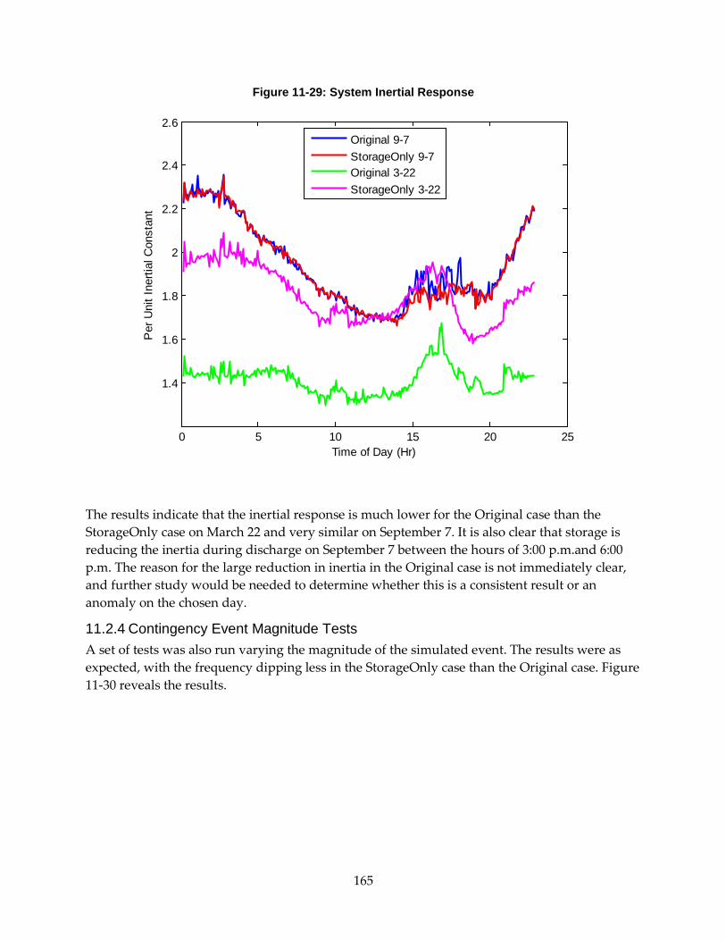
165
Figure 11-29: System Inertial Response
0 5 10 15 20 25
1.4
1.6
1.8
2
2.2
2.4
2.6
Time of Day (Hr)
Per
Uni
t Ine
rtial
Con
stan
t
Original 9-7StorageOnly 9-7Original 3-22StorageOnly 3-22
The results indicate that the inertial response is much lower for the Original case than the StorageOnly case on March 22 and very similar on September 7. It is also clear that storage is reducing the inertia during discharge on September 7 between the hours of 3:00 p.m.and 6:00 p.m. The reason for the large reduction in inertia in the Original case is not immediately clear, and further study would be needed to determine whether this is a consistent result or an anomaly on the chosen day.
11.2.4 Contingency Event Magnitude Tests A set of tests was also run varying the magnitude of the simulated event. The results were as expected, with the frequency dipping less in the StorageOnly case than the Original case. Figure 11-30 reveals the results.

166
Figure 11-30: Minimum Frequency Versus Event Size
0 2000 4000 6000 8000 10000 12000-0.8
-0.7
-0.6
-0.5
-0.4
-0.3
-0.2
-0.1
0
Event Size (MW)
Freq
uenc
y (H
z)
OriginalStorageOnly
11.2.5 Stability Assessment The results shown here demonstrate degradation in frequency response performance during high renewable days. Although, even at the highest renewable levels observed in this study, it does not appear that there would be an immediate threat to stability, there may be a gradual degradation in system performance. A more detailed and accurate system model and simulation could further characterize the threat.
Storage units appear to have a leveraged impact on the frequency stability of the system. The system reacts faster to sudden shocks. Storage units on regulation restore the system to a new stable frequency faster than would otherwise be the case, and the frequency doesn’t dip as low as it otherwise would have. Moreover, with larger storage units present on the system and charging during otherwise low load times, more generation is on-line, which can help stabilize the system in case of a contingency. If the storage units were controlled in a fashion to contribute to primary frequency response, the effect would be further amplified.
The impact of demand response on the system stability appears to be negligible, with the exception of frequency responsive loads that could potential contribute to system reserves and primary frequency response. Demand response on regulation duty appears to perform similarly to gas generators.
With increasing renewable generation will come a gradual degradation of the system frequency response. Though far from a complete assessment of all stability risks, the simulations do not indicate any exceptional issues with regard to frequency stability, other than that more concern will be warranted on days with very high renewable generation. Storage units for various functions have the ability to partially reduce this degradation and have a leveraged positive effect on system frequency stability.

167
CHAPTER 12: Summary and Conclusions Demand response (DR) and storage systems can help address an expected increase in uncertainty and variability due to high penetration of intermittent renewable generation. In day-ahead markets, they could levelize loads and prices throughout the day. They could also provide load following capability in the real-time market and regulation services to the system operator. This report assesses the value that DR and storage could provide by displacing conventional resources that would be used to provide these services in the absence of these resources. The study year is 2020. A renewable penetration goal of 33 percent was established for 2020, which was assumed to have been met.
12.1 Modeling and Data One of the key contributions of this study was the development of a high-resolution, end-to-end modeling system that includes the uncertainty in the system and how the operator could manage it. Key features include:
• Weather - A multiresolution weather model of the Western Interconnect region was used to generate the wind and solar insolation patterns that drive renewable generators. The model was run each day to generate the uncertainties over the atmospheric conditions for the following day. It includes inherent uncertainties in atmospheric physics, which result in an ensemble of possible weather trajectories rather than a point estimate and a standard deviation about that estimate. Grid scales are as small as 3 km, and results are reported at 15-minute intervals.
• Renewable generators - Wind and solar generators were placed throughout the Western Interconnect, and functions that convert wind and solar insolation into electric power were implemented. Details such as the dependence of solar photovoltaic efficiency on ambient temperature were included. Details such as wake effects in wind turbine arrays were not included.
• Net loads - Renewable generation was subtracted from gross load to obtain the net load that must be met by other resources. The daily load profiles were adjusted for the forecast temperatures so that the forecasts of load were consistent with the atmospheric forecasts. The ensemble of 30 possible weather trajectories results in an ensemble of 30 possible net load profiles. Statistical clustering techniques were used to put together this ensemble of 30 net loads to a set of five scenarios that best represent the ensemble. This collection was necessary to make the optimization problem computationally tractable.
• DR and storage data - Estimates of available DR capacity for each hour of the year were used to represent this resource. DR was categorized according to the lead time required to use the resource (day-ahead commitment, 5- minute economic dispatch, 4- second intervals for regulation). Performance parameters for Li-ion and flow batteries as well as

168
compressed air energy storage (CAES) were specified. These storage technologies could also participate in the day-ahead, 5- minute economic dispatch, and regulation markets.
• Production simulation - Production simulation logic that minimized the expected cost of operating the system given the selected weather and renewable generation trajectories was used for the analysis26F
27. The production simulation model optimally dispatches storage and demand response in concert with other system resources to meet loads. The value of storage and demand response was estimated by identifying the avoided costs of the conventional hydro and fossil resources that they displace for providing load following, frequency regulation, and peak shaving services. The PLEXOS software was used to implement and run the model.
Six simulation runs of the entire year were conducted with the model. Results were analyzed, and statistical clustering methods were used to identify 24 days that best represent the behavior of the system during the year. Thirty-four additional simulations with different combinations of DR and storage resources were run for these 24 days. Results were weighted to extrapolate the results to the full year.
The results from the weather simulation model were archived and are available for use by the renewable generation technology development community. Two hundred state variables were produced at each grid cell for each 15- minute period. It is anticipated that the data would be useful for guiding the design and siting of new wind and solar generators.
The production simulation model was run for all 5- minute periods in the year without addition of DR and storage resources. The output of this model describes the economic environment into which various DR and storage technologies could be inserted. Prices for energy and ancillary services were computed and archived for each period of the year.
12.2 Value of Demand Response and Storage The economic value of DR and storage resources that provide regulation and load following functions was assessed. Some key results of the analysis are as follows:
• DR for regulation - System operating costs were reduced by $31 million per year when DR was substituted for conventional regulation resources. These cost savings are small – about 0.3 percent of the total annual operating costs.
• DR for load following - Annual operating costs were reduced by $84 million per year, or 0.7 percent when DR was used for following load in the real-time market. Savings increased by only an additional 0.1 percent when the amount of DR capacity available was doubled but decreased by 0.3 percent when DR capacity was reduced by half. This indicates that the DR markets were becoming saturated at the assumed capacities and prices.
27 The technique is referred to as stochastic unit commitment.

169
• DR for day-ahead markets - Annual operating costs did not measurably change when the capacity is increased from 20 percent to 100 percent of the base case.
• Storage for regulation - Battery storage with 200 MW of power reduced annual operating costs by $76 million per year. These savings exceed the $60 million per year levelized capital costs for 200 MW of flywheel batteries. Flywheels would be capable of supporting the large number of charge-discharge cycles needed for regulation; it is not clear that chemical batteries could.
• Storage for energy arbitrage - Annual net revenues from the first kW of compressed air energy storage (CAES), Li-ion battery, and flow battery capacity do not cover the levelized capital costs of the batteries. Ancillary service or other revenue streams are needed to justify the investment.
• Storage power parametric study - The total storage power capacity available was varied while keeping the discharge time fixed at four hours. Net revenue showed diminishing returns to scale or market saturation effects at a total of 1,200-1,800 MW, where benefits from additional storage capacity provide little additional net revenue.
• Storage discharge time parametric study - The storage discharge capacity was held constant at 300 MW, while the discharge time was varied. Net revenue showed market saturation effects at 3 hours, where longer discharge times provide little additional net revenue.
• Storage revenues from multiple ancillary services - Hourly storage charge and discharge patterns were configured to provide energy arbitrage and ancillary services each hour of the year. Using these patterns, storage devices earned nearly $100 per kW per year from ancillary services.
12.3 Regulation and Stability High penetration of renewable generators can adversely impact stability of the system. Simulation models were used to assess how storage and demand response providing frequency regulation can reduce these impacts. Some key results are as follows:
• Frequency drop after loss of a generator - The addition of 200 MW of 15-minute storage providing regulation made the system frequency drop after a less severe generator outage (from a drop of 0.1 Hz to a drop of 0.07 Hz).
• High renewable impacts - The frequency drop after loss of a generator is worse on days when more renewable generation is on-line.
• Time-of-day effects - The frequency drop after loss of a generator is worse during early morning hours when less conventional generation is on-line and wind generation is likely to be high.
• Storage in early morning - Storage providing regulation during the early morning hours while it is charging can significantly improve performance.

170
• Sufficient energy for regulation - There is a risk that storage-providing regulation could become fully discharged or charged and be incapable of providing regulation up or down, respectively. Storage capacity of 200 MW (15 minutes) would have a 4 percent chance of reaching a charge state below 5 percent sometime during the day. The chance of being charged by more than 95 percent is less than 1 percent.
In summary, the economic values of alternative DR and storage technologies are provided in this study. The research team believes these results will be informative to policy makers seeking to establish state goals for DR and storage deployment. They also believe the models and data sets will be useful for technology developers. A technical peer review of the study is included as Appendix G. Recommendations for refinements to the model and future work are provided.

171
GLOSSARY
ACARS Aircraft Communications Addressing and Reporting System
ACE Area control error
AGC Automated generation control
Energy Commission California Energy Commission
CIEE California Institute for Energy and Environment, University of California at Berkeley
DA California Independent System Operator day-ahead market
DART Data Assimilation Research Test bed, National Center for Atmospheric Research
DFI Digital filter initialization (WRF function)
DRRC Demand Response Research Center, Lawrence Berkeley Laboratory
EV Plug in electric vehicle
FDDA Four Dimensional Data Assimilation (WRF function)
FSL Forecast Systems Laboratory (NOAA)
HPC High-performance computing systems
IOU Investor-owned utility
LBL Lawrence Berkeley Laboratory
LIDAR Light Detection and Ranging, an instrument to measure wind speed
LLNL Lawrence Livermore National Laboratory
MADIS Meteorological Assimilation Data Ingest System, maintained by NOAA
NAM North American Model, maintained by NCDC
NCDC National Climatic Data Center
NERC North American Electric Reliability Corporation
NMC National Meteorological Center
NOAA National Oceanographic and Atmospheric Administration
PG&E Pacific Gas and Electric Company

172
PIER Public Interest Energy Research Program sponsored by the California Energy Commission
PLEXOS Production simulation/optimization software developed by Energy Exemplar, LLC
PV Solar photovoltaic generator
RT California Independent System Operator real-time market
SCE Southern California Edison Company
SDG&E San Diego Gas & Electric Company
WECC Western Electricity Coordinating Council
WRF Weather Research and Forecasting Model, National Center for Atmospheric Research

173
REFERENCES
3TIER Corp., Development of Regional Wind Resource and Wind Plant Output Datasets, Subcontract Report, NREL/SR-550-47676, pg. 23, 2010.
American Public Power Association, Financial Performance of Owners of Unregulated Generation in PJM (July 2012).
Berner, J., S. Y. Ha, J. P. Hacker, A. Fournier, C. Snyder, “Model Uncertainty in a Mesoscale Ensemble Prediction System: Stochastic Versus Multiphysics Representations,” Monthly Weather Review 139, pp. 1972–1995, 2011.
Bowden, Jared H., Tanya L. Otte, Christopher G. Nolte, Martin J. Otte, “Examining Interior Grid Nudging Techniques Using Two-Way Nesting in the WRF Model for Regional Climate Modeling,” Journal of Climate, 25, pp. 2805–2823, 2012.
California Independent System Operator Corporation, Integration of Renewable Resources: Technical Appendices for California ISO Renewable Integration Studies, Version 1, October 2010.
California Wind Resources - Draft Staff Paper by Dora Yen-Nakafuji, CEC-500-2005-071-D, April 2005, http://www.energy.ca.gov/wind/windfacts.html
2020 Strategic Analysis of Energy Storage in California, CEC-500-2011-047, November 2011.
Cibulka, Lloyd, Merwin Brown, Larry Miller, Alexandra Von Meier, User Requirements and Research Needs for Renewable Generation Forecasting Tools That Will Meet the Needs of the CAISO and Utilities for 2020, California Institute for Energy and Environment, September 2012.
“NCAR Wind Forecasting System Saves Millions for Xcel Energy,” Colorado Energy News, November 14, 2011, http://coloradoenergynews.com/2011/11/ncar-wind-forecasting-system-saves-millions-for-xcel-energy/
Corder, G.W and D. I. Foreman, Nonparametric Statistics for Non-Statisticians: A Step-by-Step Approach, Wiley, 2009.
Dupacova, J., N. Growe-Kuska and W. Romisch, “Scenario Reduction in Stochastic Programming: An Approach Using Probability Metrics.” Math Programming 95, pp. 493-511, 2003.
Eckel, F. A. and C. F. Mass, “Aspects of Effective Mesoscale, Short-Range, Ensemble Forecasting,” Weather Forecasting 20, pp. 328–350, 2005.
U.S. Energy Information Administration, Assumptions to the Annual Energy Outlook 2012, August 2012.
Electric Power Research Institute, Cost-Effectiveness of Energy Storage in California, EPRI-3002001162, June 2013.

174
Hacker, J. P., S. Y. Ha, C. Snyder, J. Berner, F. A. Eckel, E. Kuchera, M. Pocernich, S. Rugg, J. Schramm, and X. Wang, “The U.S. Air Force Weather Agency's Mesoscale Ensemble: Scientific Description and Performance Results.” Tellus 63A, pp. 625-641, 2011.
Hartigan, J.A. and M. A. Wong, “A K-Means Clustering Algorithm,” Applied Statistics 28, pp. 100–108, 1979.
Hou, D., E. Kalnay, and K. Drogemeier, “Objective Verification of the SAMEX ’98 Ensemble Experiments,” Monthly Weather Review 129, 73–91, 2001.
[KEMA 2010] DNV KEMA, Inc., Research Evaluation of Wind Generation, Solar Generation, and Storage Impact on the California Grid, PIER Project CEC-500-2010-010, June 2010.
DNV KEMA Corporation, Energy Storage Cost-Effectiveness Methodology and Preliminary Results (DRAFT), June 2013.
Lamont 2013, A. Lamont, “Assessing the Economic Value and Optimal Structure of Large-Scale Electricity Storage,” IEEE Transactions on Power Systems, Vol. 28, No. 2, pp. 911-921, May 2013.
Lew, D., M. Milligan, D. Piwko, and G. Jordon, “The Value of Wind Power Forecasting, Second Conference on Weather, Climate, and the New Energy Economy, Seattle, WA,” American Meteorological Society, 2.1. D.12-12-031, pg. 82, 2011.
Liu, Y., A. Bourgeois, T. Warner, S. Swerdlin and J. Hacker, An Implementation of Obs-Nudging-Based FDDA Into WRF for Supporting ATEC Test Operations, 2005 WRF User Workshop, Paper 10.7, 2005.
Lo, J. C. F., Z. L. Yang, and R. A. Pielke Sr., “Assessment of Three Dynamical Climate Downscaling Methods Using the Weather Research and Forecasting (WRF) Model,” Journal of Geophysical Research 113, D09112, doi:10.1029/2007JD009216, 2008.
Meibom, Peter, Rudiger Barth, Ian Norheim, Hans Ravn, and Poul Sorensen, Wind Integration in a Liberalized Electricity Market, Risoe National Laboratory, 2006.
Miller, P.A., M. Barth, L. Benjamin, D. Helms, M. Campbell, J. Facundo, and J. O'Sullivan, “The Meteorological Assimilation and Data Ingest System (MADIS): Providing Value-added Observations to the Meteorological Community,” 21st Conference on Weather Analysis and Forecasting, Washington, D.C., American Meteorological Society, 2005.
Miller, P.A., M.F. Barth, L.A. Benjamin, A 2009 “Update on the NOAA Meteorological Assimilation Data Ingest System (MADIS),” 25th Conference on International Interactive Information and Processing Systems (IIPS) for Meteorology,Oceanography, and Hydrology, Phoenix, AZ, American Meteorological Society, 2009.
Mullen, S. L., and D. P. Baumhefner, “Monte Carlo Simulations of Explosive Cyclogenesis,” Monthly Weather Review 122, pp. 1548–1567, 1994.

175
Murphy, J., D. Sexton, D. Barnett, G. Jones, M. Webb, M. Collins, and D. Stainforth, “Quantification of Modeling Uncertainties in a Large Ensemble of Climate Change Simulations,” Nature 430, pp. 768–772, 2004.
National Renewable Energy Laboratory, Cost and Performance Data for Power Generation Technologies, prepared for National Renewable Energy Laboratory by Black and Veatch, February 2012.
National Renewable Energy Laboratory, The Value of Storage for Grid Applications, NREL/TP-6A20-58465, May 2013.
Otte, Tanya L., “The Impact of Nudging in the Meteorological Model for Retrospective Air Quality Simulations, Part I: Evaluation Against National Observation Networks,” Journal of Applied Meteorology and Climatology 47, pp. 1853–1867, 2008.
K. Parks, Y-H. Wan, G. Wiener, and Y. Liu, Wind Energy Forecasting: A Collaboration of the National Center for Atmospheric Research (NCAR) and Xcel Energy, NREL NREL/SR-5500-52233, Golden, CO: National Renewable Energy Laboratory, 2011.
A. Papavasiliou, S. S. Oren, “Multi-Area Stochastic Unit Commitment for High Wind Penetration in a Transmission Constrained Network,” submitted to Journal of Operations Research, July 2012.
PLEXOS software is a product of Energy Exemplar, LLC, http://www.energyexemplar.com/
Rothleder, Mark, Track I Direct Testimony of Mark Rothleder on Behalf of the California Independent System Operator Corporation, California Public Utilities Commission Rulemaking 10-05-006, July 2011.
Salathé, E. P., R. Steed, C. F. Mass, and P. H. Zahn, A High-Resolution Climate Model for the U.S. Pacific Northwest: Mesoscale Feedbacks and Local Responses to Climate Change,” Journal of Climate 21, pp. 5708–5726, 2008.
California Senate Bill No. 2, April 12, 2011.
Simpson, Matthew, Sonia Wharton, and Wayne Miller, Validation of a Short-Range Ensemble Forecast of a Wind Ramp Event With LIDAR Measurements, LLNL-PRES-575574, August 2012.
Sioshansi, et al, 2009, R. Sioshansi, P. Denholm, T. Jenkin, J. Weiss, “Estimating the Value of Electricity Storage in PJM: Arbitrage and Some Welfare Effects,” Energy Economics 31, 2009, pp. 269–277, 2009.
Skamarock, W. C., J. B. Klemp, J. Dudhia, D. O. Gill, D. M. Barker, M. Duda, X.-Y. Huang, W. Wang and J. G. Powers, A Description of the Advanced Research WRF Version 3, National Center for Atmospheric Research, 2008, http://www.mmm.ucar.edu/wrf/users/docs/arw_v3.pdf

176
Stauffer, D. R., and N. L. Seaman, “Use of Four-Dimensional Data Assimilation in a Limited-Area Mesoscale Model, Part I: Experiments With Synoptic-Scale Data,” Monthly Weather Review 118, pp. 1250-1277, 1990.
Stauffer, D. R., and N.L. Seaman, “On Multi-Scale Four-Dimensional Data Assimilation,” Journal of Applied Meteorology 33, pp. 416-434, 1994.
Stensrud, D., J. W. Bao, and T. T. Warner, “Using Initial Condition and Model Physics Perturbations in Short-Range Ensemble Simulations of Mesoscale Convective Systems,” Monthly Weather Review 128, pp. 2077–2107, 2000.
Tuohy and O’Mally 2011, A. Tuohy, M. O’Mally, “Pumped Storage in Systems With Very High Wind Penetration,” Energy Policy 39, pp.1965 – 1974, 2011.
V90-3.0 MW, “An Efficient Way to More Power,” Vestas Wind Systems A/S, www.vestas.com

A-1
APPENDIX A: Solar and Wind Sites Used in Weather Model
Table A-1: Proposed Large-Scale Solar Photovoltaic Power Plants
Name WRF Domain MW
Carrizo_South_PV_1 d02 150
Carrizo_South_PV_2 d02 400
Carrizo_South_PV_3 d02 350
Fairmont_PV_1 39
Imperial_PV_1 d04 174
Mountain_Pass_PV_1 d04 300
Non_CREZ_PV_1 d02 50
Non_CREZ_PV_2 d02 232
Pisgah _PV_1 d04 75
Riverside_East_PV_1 d04 300
Riverside_East_PV_2 d04 250
Tehachapi_PV_1 d04 341
Tehachapi_PV_2 d04 341
Tehachapi_PV_3 d04 341
Tehachapi_PV_4 d04 341
Arizona_PV_1 d04 290
Arizona_PV_2 d04 50
Total 4,024

A-2
Table A-2: Proposed Solar Thermal Power Plants
Name WRF Domain MW
Imperial_ST_1 d04 300
Kramer_ST_1 d04 62
Mountain_Pass_ST_1 d04 110
Mountain_Pass_ST_2 d04 300
Non_CREZ_ST_1 d04 150
Non_CREZ_ST_2 d04 370
Pisgah_ST_1 d04 250
Pisgah_ST_2 d04 250
Pisgah_ST_4 d04 400
Pisgah_ST_5 d04 400
Pisgah_ST_6 d04 400
Riverside_East _ST_1 d04 250
Riverside_East _ST_2 d04 242
Tehachapi_ST_1 d04 105
Arizona_ST_1 d04 200
Arizona_ST_2 d04 200
Total 3,989
Table A-3: Proposed Small Solar Power Plant Data
Plant Name WRF
Domain
# WRF Gridcells MW
Distributed_Solar_1 d03 648 350
Distributed_Solar_2 d02 182 350
Distributed_Solar_3 d03 1021 350
Distributed_Solar_4 d04 1077 350
Distributed_Solar_5 d04 374 350
Total 1,750

A-3
Table A-4: Existing and Proposed Distributed Solar Power Plant Data
Plant Name Status WRF
Domain
# of WRF Gridcells MW
Large_Roof_3 Existing d04 395 99
Large_Roof_8 Existing d04 567 335
Large_Ground_1 Proposed 407
Large_Ground_8 Proposed d04 180 120
Large_Ground_12 Proposed d03 323 89
Large_Roof_8 Proposed d04 567 430
Total Existing
434
Total Proposed 1,046

A-4
Table A-5: Existing and Proposed Wind Power Plant Data
Plant Name Existing or Proposed
In or Out Of State
WRF
Domain
# of WRF Gridcells MW
Altamont Existing In State d03 16 682
Solano Existing In State d03 6 200
San Gorgonio Existing In State d04 9 391
Tehachapi Existing In State d04 16 774
Imperial_W1 Proposed In State d04 8 595
Mountain_Pass_W Proposed In State d04 3 178
Palm_Springs_W2 Proposed In State d04 1 77
San_Bernardino_Lucerne_W1 Proposed In State d04 2 120
San_Diego_South_W1 Proposed In State d04 5 379
Solano_W1 Proposed In State d03 8 657
Solano_W2 Proposed In State d03 6 469
Tehachapi_W1 Proposed In State d04 9 710
Tehachapi_W2 Proposed In State d04 9 750
Tehachapi_W3 Proposed In State d04 9 750
Tehachapi_W4 Proposed In State d04 10 764
Alberta_W1 Proposed Out Of State d01 1 436
Alberta_W2 Proposed Out Of State d01 1 450
Colorado_W1 Proposed Out Of State d01 1 420
Montana_W Proposed Out Of State d01 1 300
Northwest_W1 Proposed Out Of State d02 1 420
Northwest_W2 Proposed Out Of State d01 1 750
Northwest_W3 Proposed Out Of State d01 1 539
Northwest_W4 Proposed Out Of State d02 1 204
Northwest_W5 Proposed Out Of State d02 1 442
Utah_W2 Proposed Out Of State d02 1 104
Wyoming_W1 Proposed Out Of State d01 1 96
Total Existing 2,047
Total Proposed 9,610
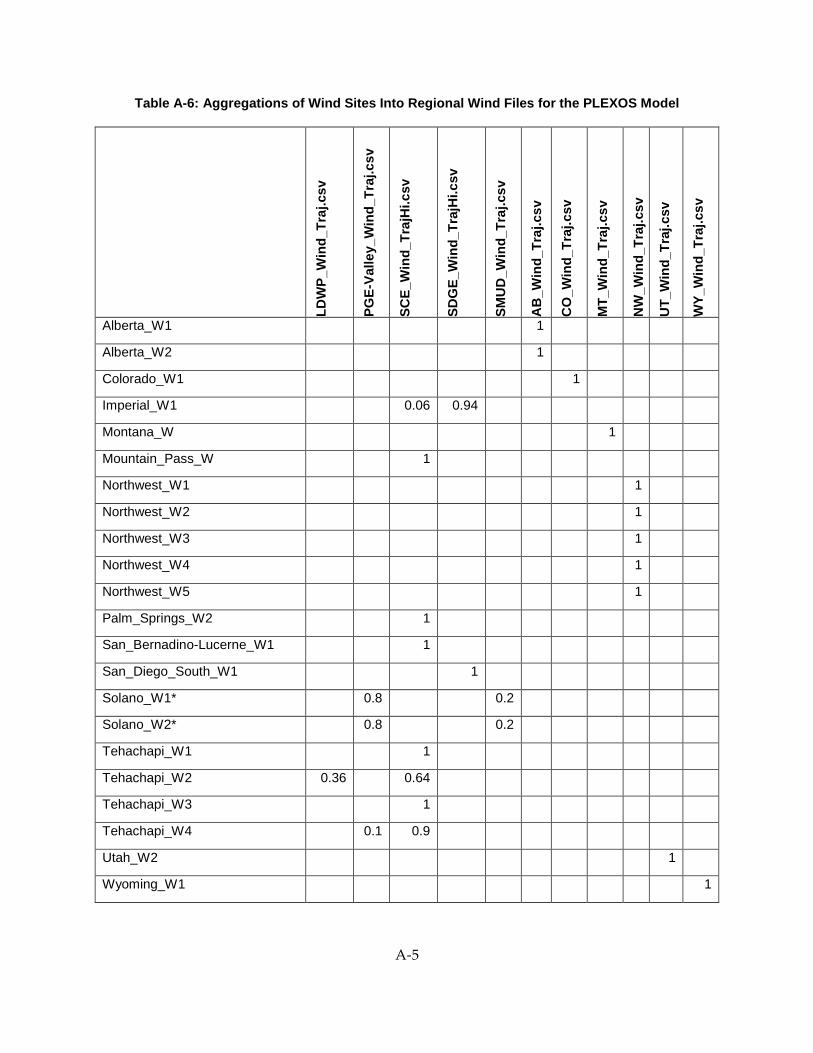
A-5
Table A-6: Aggregations of Wind Sites Into Regional Wind Files for the PLEXOS Model
LDW
P_W
ind_
Traj
.csv
PGE-
Valle
y_W
ind_
Traj
.csv
SCE_
Win
d_Tr
ajH
i.csv
SDG
E_W
ind_
Traj
Hi.c
sv
SMU
D_W
ind_
Traj
.csv
AB
_Win
d_Tr
aj.c
sv
CO
_Win
d_Tr
aj.c
sv
MT_
Win
d_Tr
aj.c
sv
NW
_Win
d_Tr
aj.c
sv
UT_
Win
d_Tr
aj.c
sv
WY_
Win
d_Tr
aj.c
sv
Alberta_W1 1
Alberta_W2 1
Colorado_W1 1
Imperial_W1 0.06 0.94
Montana_W 1
Mountain_Pass_W 1
Northwest_W1 1
Northwest_W2 1
Northwest_W3 1
Northwest_W4 1
Northwest_W5 1
Palm_Springs_W2 1
San_Bernadino-Lucerne_W1 1
San_Diego_South_W1 1
Solano_W1* 0.8 0.2
Solano_W2* 0.8 0.2
Tehachapi_W1 1
Tehachapi_W2 0.36 0.64
Tehachapi_W3 1
Tehachapi_W4 0.1 0.9
Utah_W2 1
Wyoming_W1 1

A-6
Table A-7: Aggregations of Large PV Sites Into Regional Files for the PLEXOS Model
AZ_
LgPV
_Tra
j.csv
NV_
LgPV
_Tra
j.csv
PGE-
Valle
y_Lg
PV_T
raj.c
sv
SCE_
LgPV
_Tra
jHi.c
sv
SDG
E_Lg
PV_T
rajH
i.csv
Arizona_PV_1 1
Arizona_PV_2 1
Carrizo_South_PV_1 1
Carrizo_South_PV_2 1
Carrizo_South_PV_3 1
Fairmont_PV_1 1
Imperial_PV_1 1
Mountain_Pass_PV_1 1
NonCREZ_PV_1 1
NonCREZ_PV_2 1
Pisgah_PV_1 1
Riverside_East_PV_1 1
Riverside_East_PV_2 1
Tehachapi_PV_1 1
Tehachapi_PV_2 1
Tehachapi_PV_3 1
Tehachapi_PV_4 1

A-7
Table A-8: Aggregations of Solar Thermal Sites Into Regional Files for the PLEXOS Model
LDW
P_ST
_Tra
j.csv
NEV
P_ST
_Tra
j.csv
SCE_
ST_T
raj.c
sv
SDG
E_ST
_Tra
j.csv
Arizona_ST_1 1
Arizona_ST_2 1
Imperial_ST_1 1
Kramer_ST_1 1
Mountain_Pass_ST_1 1
Mountain_Pass_ST_2 1
NonCREZ_ST_1 1
NonCREZ_ST_2 1
Pisgah_ST_1 1
Pisgah_ST_2 1
Pisgah_ST_4 1
Pisgah_ST_5 1
Pisgah_ST_6 1
Riverside_East_ST_1 1
Riverside_East_ST_2 1
Tehachapi_ST_1 1

A-8
Table A-9: Aggregations of Small PV Sites into Regional Files for the PLEXOS Model
PGE-
Bay
_Sm
PV_T
raj.c
sv
PGE-
Valle
y_Sm
PV_T
raj.c
sv
SCE_
SmPV
_Tra
j.csv
SDG
E_Sm
PV_T
raj.c
sv
Large_Ground_1 1
Large_Ground_8 1
Large_Ground_12 1
Large_Roof_8 0.88 0.12
Table A-10: Aggregations of Distributed Solar Sites into Regional PLEXOS Files
LDW
P_D
GPV
_Tra
j.csv
PGE-
Bay
_DG
PV_T
raj.c
sv
PGE-
Valle
y_D
GPV
_Tra
j.csv
SCE_
DG
PV_T
raj.c
sv
SDG
E_D
GPV
_Tra
j.csv
SMU
D_D
GPV
_Tra
j.csv
Distributed_Solar_1 0.92 0.08
Distributed_Solar_2 0.66 0.34
Distributed_Solar_3 1
Distributed_Solar_4 0.51 0.49
Distributed_Solar_5 0.54 0.46

B-1
APPENDIX B: Example Net Load Trajectories California ISO net load trajectories for Monday, April 6, through Sunday, April 12, 2020. Selected trajectories are shown in color. Line width is proportional to the probability assigned to the trajectory.

B-2

B-3
California ISO net load trajectories for Monday, August 3, through Sunday, August 9, 2020. Six selected trajectories are shown in color. Line width is proportional to the probability assigned to the trajectory.

B-4

B-5
California ISO net load trajectories for Monday, November 9, through Sunday, November 15, 2020. Six selected trajectories are shown in color. Line width is proportional to the probability assigned to the trajectory.
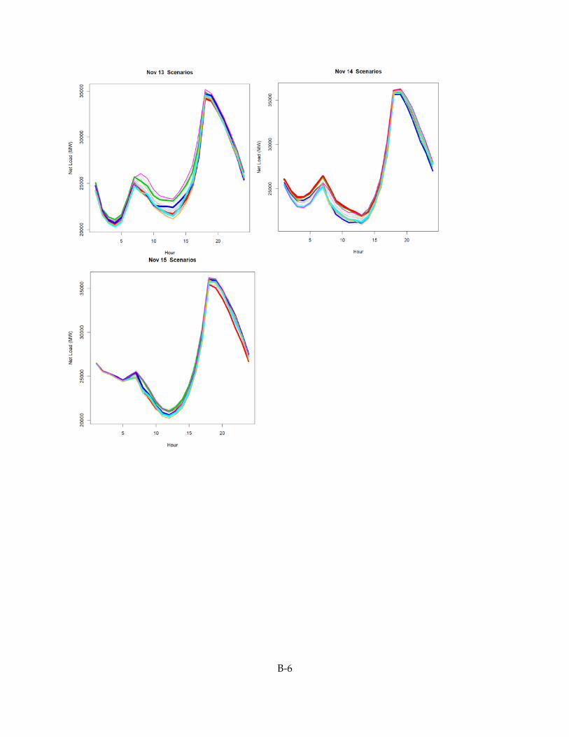
B-6

B-7
California ISO net load trajectories for Monday, February 10, through Sunday, February 16, 2020. Six selected trajectories are shown in color. Line width is proportional to the probability assigned to the trajectory.

B-8

C-1
APPENDIX C: Demand Response Programs and Data Overview of Current Demand Response Programs at Pacific Gas and Electric Company The Pacific Gas and Electric Company has a range of demand response programs in place. Programs offered may evolve by 2020 and may differ by utility. A brief summary of the programs is provided in Table C-1.
Table C-1: PG&E Current Demand Response Programs
Program Name How It Works Incentives
Base Interruptible Program (BIP)27F
28
The BIP pays an incentive to reduce load to or below a level that is pre-selected by the customer. This pre-selected level is called the Firm Service Level (FSL).
BIP gives 30 minutes advance notice to curtail in exchange for a monthly incentive payment even if no events are called. However, failure to reduce load down to or below FSL during an event will result in a charge of $6.00/kWh for any energy use above the FSL. There is a maximum of one event per day and four hours per event. The program will not exceed 10 events per month, or 120 hours per year.
Monthly bill credit is based on potential load reduction (PLR). During summer months, the PLR is the difference between that month's average on-peak demand (on-peak kWh divided by the number of on-peak hours) and FSL. During winter months, the PLR is based upon partial-peak demand. Monthly incentives are: PLR Incentive <500 kW $8 per kW 501 kW - 1 MW $8.50 per kW >1MW $9 per kW Customers may also elect to participate in PG&E's Under Frequency Relay (UFR) program with an additional monthly incentive of $0.67/kW.
Demand Bidding Program (DBP)28F
29
DBP pays an incentive to reduce load when notified of a DR event day by PG&E. This is a
For day-ahead events, customer will receive an event notice by noon on the business day before the planned event. Customer will have until 3 p.m. that day to submit bids via
The incentive rate is $0.50/kW per hour for day-ahead events and $0.60/kW per hour for day-of events. Hour-by-hour load reduction will be determined as the difference
28 http://www.pge.com/mybusiness/energysavingsrebates/demandresponse/baseinterruptible/
29 http://www.pge.com/mybusiness/energysavingsrebates/demandresponse/dbp/

C-2
Program Name How It Works Incentives
relatively low-risk DR program that allows customers to submit load reduction bids for a DBP event, which can be called on a day-ahead or day-of basis. For any event, customer may elect to submit or not submit a bid. If a bid is submitted, customer can still choose to forgo reducing load without penalty.
InterAct, PG&E's Internet-based customer interface.
For day-of events, customer will have one hour after receiving the event notice to submit bids via InterAct. PG&E will notify participants of bid acceptance within 15 minutes of the bid acceptance window closing.
The bid must be for a minimum of two consecutive hours within the planned event window and must meet a minimum reduction of 50 kilowatts (kW) each hour.
between a baseline and actual electric usage during the event. The baseline is determined by calculating the energy usage of the prior 10 days to the curtailment event day.
Optional Binding Mandatory Curtailment (OBMC) Plan29F
30
This program avoids rotating outages in high demand periods by reducing the entire electric circuit load of the facility.
PG&E will notify customer of required load reduction (5 to 15 percent) and give customer start and end times of the event, which will: • Occur on any day
(holidays and weekends included) without limitations to frequency and duration.
• Exempt customer from “block progression” rotating outages.
• Require customer to submit a load-reduction plan each year.
There are no financial incentives for participating in OBMC. The benefit is exemption from rotating outages. However, if customer is not able to reduce load to the level specified in each notice, there are penalties: • $6 penalty for each kWh
above power reduction commitment.
• Plan termination for failure to reduce load a second time during a 1-year period.
• OBMC participation denied for a period of five years after termination.
Scheduled Load Reduction Program (SLRP)30F
31
Program pays to reduce load by pre-selected amounts during pre-selected time periods
Customer selects one to three four-hour periods (between 8 a.m. to 8 p.m.) on one or more weekdays. Customer is required to reduce load each and every time Load reduction cannot be shifted to an on-peak period (noon to 6 p.m.) on another day. • The committed load
The program will pay $0.10/kWh per month (June through September) for actual energy reductions.
Actual energy reductions are the difference between a baseline calculated using non-SLRP days and actual energy usage during SLRP hours on
30 http://www.pge.com/mybusiness/energysavingsrebates/demandresponse/obmcp/
31 http://www.pge.com/mybusiness/energysavingsrebates/demandresponse/slrp/

C-3
Program Name How It Works Incentives
reduction must be at least 15 percent of average monthly demand or 100 kW, whichever is greater.
• Load reductions are measured relative to a baseline that is specific to customer’s facility.
SLRP days.
Smart AC for homeowners31F
32
The SmartAC program offers the opportunity to help prevent summer energy supply emergencies from disrupting day to day activities.
PG&E will install a free SmartAC device. If there is an energy supply emergency, between May 1 and October 31, the SmartAC device will receive a signal to use slightly less power to help avoid power interruptions.
Customer will receive $50 from PG&E after installation of a SmartAC device.
Demand Response Capacity Forecast for 2020 Representatives of the Demand Response Research Center provided estimates of demand response availability for each hour of the year. A typical data set is shown in the figure below, which identifies the sources of DR capacity.
32 http://www.pge.com/en/myhome/saveenergymoney/energysavingprograms/smartac/index.page, http://www.pge.com/en/myhome/saveenergymoney/energysavingprograms/smartac/faq/index.page

C-4
Figure C-1: SCE Demand Response Availability by Source on August 2, 2020
0 5 10 15 20 250
100
200
300
400
500
600
700
Hour
DR
Max
imum
Ava
ilabi
lity
(MW
)
comm_coolingcomm_lightingcomm_ventout_lightres_coolingres_water
The data in the figure below show forecasts of the types of demand response that would be offered during each hour of the day on August 2, 2020. The data in the figure indicate that firm demand response, which is committed and dispatched in the day-ahead market, is the largest resource. This type of DR is referred to as economic DR in the production simulation model. Flexible demand response is offered at 5-minute economic dispatch intervals and can be used for load following. This type of DR is referred to as load following DR in the PLEXOS model. Regulation demand response reacts to 4- second automated generator control signals. This type of demand response is not modeled in the production simulation model. Regulation DR capacity is subtracted from the regulation requirements file that is used as input to the production simulation model.

C-5
Figure C-2: SCE Demand Response Availability by Application on August 2, 2020
0 5 10 15 20 25200
400
600
800
1000
1200
1400
1600
1800
2000
Hour
DR
Max
imum
Ava
ilabi
lity
(MW
)
y y pp g
firmflexreg
The data in the figure below show forecasts of the types of demand response as a percentage of Southern California Edison’s load in each hour of the day on August 2, 2020. The data in the figure indicate that economic demand response committed and dispatched in the day-ahead market is the largest resource. Load following demand response dispatched in the real-time market is the second largest resource.
Figure C-3: SCE Demand Response Availability by Application as a Percentage of Total Load
0 5 10 15 20 252
4
6
8
10
12
14
16
18
Hour
DR
Max
imum
Ava
ilabi
lity
(%)
y y pp g ,
firmflexreg

C-6
The data in the figure below illustrate the seasonality of demand response availability. The data indicate about 50 percent more demand response is available during the summer days in Southern California Edison’s service territory.
Figure C-4: Demand Response Available per Day in California
0 50 100 150 200 250 300 350 4001600
1800
2000
2200
2400
2600
2800
3000
3200
3400
3600
Day
Ene
rgy
Ava
ilabl
e (M
Wh)
gy p y
Some fraction of the DR is available and capable of providing regulation up and down services. The availability of DR to provide regulation up is shown in the figure below. As indicated by the data in the figure, small amounts of DR are available to provide regulation up in the middle of the day when other loads are being serviced. There is a big increase in DR availability during and after the evening peak throughout the year. The patterns for regulation down availability are similar – large amounts of capacity are available during and after the evening peak. During these periods, apparently DR participants have some freedom to modulate load in response to regulation signals.

C-7
Figure C-5: Demand Response Available for Regulation Up
MW
Finally, the DR capacity available for commitment in the day-ahead market is shown in the figure below. The horizontal lines in the figure correspond to weekends when less DR is available. Large amounts of DR are available during summer peak loads.

C-8
Figure C-6: Demand Response Available for Five-Minute Economic Dispatch
MW
Finally, the DR capacity available for commitment in the day-ahead market is shown in the figure below. The horizontal lines in the figure correspond to weekends when less DR is available. Large amounts of DR are available during summer peak loads.

C-9
Figure C-7: Demand Response Available for Commitment in the Day-Ahead Market
MW
The DRRC was unable to provide prices associated with these projected capacities. The prices in the California ISO model of the High Load scenario were set to values in three tiers of $1,000/MWh, $600/MWh, and $136/MWh, respectively. It was noted that DR at these prices was seldom dispatched, so prices were changed to $130/MWh, $105/MWh, and $80/MWh. These changes in prices caused DR to be dispatched over the seasons in a manner closely aligned to the specifications for the California ISO demand response product. California ISO allows bid-in demand response to be dispatched 15 times for a total of 48 hours each season (winter and summer). As follow-up work to this study, it would be interesting for the DRRC to determine if these prices that would make DR competitive with other system resources are consistent with the DR capacities they provided (that is, would these prices support infrastructure development and provide sufficient incentives for program participation).

D-1
APPENDIX D: Storage Data Representatives of the Electric Power Research Institute and the California Energy Storage Alliance provided estimates of storage technology cost and performance characteristics via private communication. A summary of the data provided is shown in the table. Data sheets for each of the storage technologies are also provided.
Table D-1: Summary of Storage Technology Cost and Performance Parameters
Technology
MW
MWh
Capital Cost ($M)
Specific Capital Cost ($M/ MW)
Specific Energy
Cost ($M/ MWh)
Var. O&M
($/ MWh)
Plant Life
(yrs.)
Cycles @ 80% DOD
Cycles @ 5% DOD
Round
Trip Eff. (%)
Li-Ion battery (15 min)
2 0.5 2.5 1.25 5 0.25* 15 10,000 100,000
83
Li-Ion Battery (4hr)
1 4 3.6 3.6 0.9 0.25* 15 5,000 85
Flow Battery (5 hr.)
50 250 93 1.86 0.372 0.25* 15 65
Flywheel (15 min)
20 5 38 1.9 7.6 0 25 Infinite Infinite 87
Compressed Air Above Ground (5 hr.)
50 250 100 2 0.4 6 35 Infinite Infinite 70
Compressed Air Below Ground (10 hr.)
200 2,000 300 1.5 0.15 6 35 Infinite Infinite 70
Source: CPUC data sheet provided by Aloke Gupta on Feb. 8, 2013. O&M costs for flow battery assumed to apply to Li-ion batteries.

D-2
Technology: Medium duration Li-ion energy storage systems (1MW/ 2-4hr class) Person providing information: Ben Kaun Email:[email protected] Phone: 650-855-2208 Organization: EPRI Configurations of Capacity: EPRI Input CESA Comments Can the charging and discharging capacity be sized separately from the amount of energy stored? What are the considerations in developing installations with different ratios of discharge capacity to energy capacity?
Yes, flexibly in the 1:1 to 1:4 Power to energy ratio range
Agreed
Power/Energy Ratio: What is a typical ratio for this technology (may include a set of several ratios)?
1:2 to 1:4 Agreed
Efficiency: What is the round-trip efficiency? 80-85% would be typical 85% Life: What is the operating life in years, or numbers of cycles?
10-15 years, 5000 cycles to 80% DOD typical
Agreed
What is the relationship between depth of discharge and life?
Strong relationship, depending on specific chemistry. CESA to provide sample DOD relationship?
Agreed
Operating Parameters: What is the response time to start generating or charging?
Milliseconds to seconds Agreed
How much time after start does it take to reach full output?
Milliseconds to seconds Agreed
Are there any restrictions on partial output (is there a minimum power level)?
No Agreed
Are there any restrictions on call frequency (per 4 sec, 5 minutes, hour, day, or month)?
No Agreed

D-3
Costs32F
33: Li-ion 1MW/2hour = $2.5M; Li-ion 1MW/4hour = $3.6M
Li-ion 1MW/2hour = $2.2M; Li-ion 1MW/4hour = $3.6M
What are the capital costs of charging and discharging capacity ($/MW)?
TBD CESA Replacements of cell stacks in $/kWh only. See below.
What are the capital costs of energy storage capacity ($/MWh)?
TBD CESA About $500-750/kWh cell stack replacement costs33F34
What are the costs of small units versus cost of large units (e.g., are there returns to scale in building large units)?
Yes, but not huge differences in the 1MW to 50MW range. Perhaps 10-20% savings going from 1MW to 50 MW?
Agreed
Are there any variable operating costs ($/MWh discharged or charged)?
Insufficient track record. Placeholder of $0.001 - $0.005/kWh?
$2/kW-yr. fixed O&M (Assumes $2,800/yr. of planned maintenance for a 1,400kWh ESS (40h/yr. at $70/h for technician)) $0.01/kWh discharged (Assumes approximately 0.4% of cells will be replaced each year due to unplanned failures)
Technology: Short duration Li-ion energy storage systems (2MW/ 15-min class) Person providing information: Ben Kaun Email:[email protected] Phone: 650-855-2208 Organization: EPRI
Configurations of Capacity: EPRI Input CESA Comments Can the charging and discharging capacity be sized separately from the amount of energy stored? What are the considerations in developing
Yes, within the range of 4:1 to 2:1
Agreed
33 Costs for a demonstration plant in 2012 with cost reductions extrapolated to 2020 based upon technology maturation due to demand from electric vehicle market.
34 EPRI indicated that this replacement cost looks high. Would expect costs to range $300-500/kWh, and should be lower cost per unit energy than 15-min battery.

D-4
installations with different ratios of discharge capacity to energy capacity? Power/Energy Ratio: What is a typical ratio for this technology (may include a set of several ratios)?
4:1 to 2:1 Agreed
Efficiency: What is the round-trip efficiency? 80-85% would be a
typical range 85%
Life: What is the operating life in years, or numbers of cycles?
10-15 years dependent on usage, 5000-10,000 cycles to 80% DOD typical
Agreed
What is the relationship between depth of discharge and life?
Strong relationship, depending on specific chemistry. At shallow DOD, maybe get over 100k cycles (5-10% DOD)
Agreed
Operating Parameters: What is the response time to start generating or charging?
Milliseconds to seconds
Agreed
How much time after start does it take to reach full output?
Milliseconds to seconds
Agreed
Are there any restrictions on partial output (is there a minimum power level)?
No Agreed
Are there any restrictions on call frequency (per 4 sec, 5 minutes, hour, day, or month)?
No No, assuming this means how often the device can be called upon to adjust its output
Costs34F
35: $2.5M for 2MW, 0.25h What are the capital costs of charging and discharging capacity ($/MW)?
Replacements of cell stacks in $/kWh only. See below.
What are the capital costs of energy storage capacity ($/MWh)?
About $500-750/kWh cell stack replacement costs
35 Costs for a demonstration plant in 2013. LLNL assumes an annual cost reduction rate of 5 percent per year, which implies costs in 2020 would be lower by a factor of (1-0.05)7 = 0.70.

D-5
What are the costs of small units versus cost of large units (e.g., are there returns to scale in building large units)?
Unknown For small community energy storage units of ~50kW, the $/kW system cost is substantially higher than ~1MW scale systems
Are there any variable operating costs ($/MWh discharged or charged)?
Insufficient track record. Placeholder of $0.001 - $0.005/kWh
$2/kW-yr. fixed O&M (Assumes $2,800/yr. of planned maintenance for a 1,400kWh ESS (40h/yr. at $70/h for technician))
$0.01/kWh discharged (Assumes approximately 0.4% of cells will be replaced each year due to unplanned failures)
Technology: Long-duration bulk flow battery (50MW/ 5hr class)
Person providing information: Ben Kaun Email:[email protected] Phone: 650-855-2208 Organization: EPRI Description of technology: Based on zinc-bromide
Configurations of Capacity: Can the charging and discharging capacity be sized separately from the amount of energy stored? What are the considerations in developing installations with different ratios of discharge capacity to energy capacity?
Yes, as long as the ratio is lower than 1:4 or 1:5
Power/Energy Ratio: What is a typical ratio for this technology (may include a set of several ratios)?
1:5 to 1:8
Efficiency: What is the round-trip efficiency? 65%
Life: What is the operating life in years, or numbers of cycles?
15 years?
What is the relationship between depth of discharge and life?
Unknown, but expected to be minimal. Failure may be better predicted by total hours of operation.
Operating Parameters:
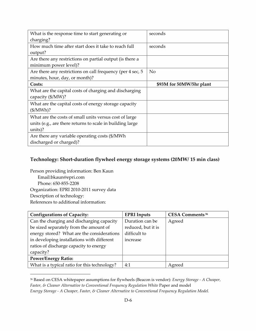
D-6
What is the response time to start generating or charging?
seconds
How much time after start does it take to reach full output?
seconds
Are there any restrictions on partial output (is there a minimum power level)?
Are there any restrictions on call frequency (per 4 sec, 5 minutes, hour, day, or month)?
No
Costs: $93M for 50MW/5hr plant What are the capital costs of charging and discharging capacity ($/MW)?
What are the capital costs of energy storage capacity ($/MWh)?
What are the costs of small units versus cost of large units (e.g., are there returns to scale in building large units)?
Are there any variable operating costs ($/MWh discharged or charged)?
Technology: Short-duration flywheel energy storage systems (20MW/ 15 min class)
Person providing information: Ben Kaun Email:[email protected] Phone: 650-855-2208 Organization: EPRI 2010-2011 survey data Description of technology: References to additional information: Configurations of Capacity: EPRI Inputs CESA Comments35F
36 Can the charging and discharging capacity be sized separately from the amount of energy stored? What are the considerations in developing installations with different ratios of discharge capacity to energy capacity?
Duration can be reduced, but it is difficult to increase
Agreed
Power/Energy Ratio: What is a typical ratio for this technology? 4:1 Agreed
36 Based on CESA whitepaper assumptions for flywheels (Beacon is vendor): Energy Storage - A Cheaper, Faster, & Cleaner Alternative to Conventional Frequency Regulation White Paper and model Energy Storage - A Cheaper, Faster, & Cleaner Alternative to Conventional Frequency Regulation Model.
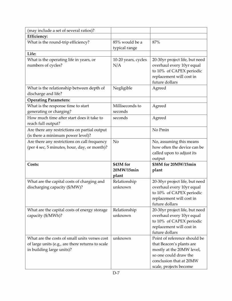
D-7
(may include a set of several ratios)? Efficiency: What is the round-trip efficiency? 85% would be a
typical range 87%
Life: What is the operating life in years, or numbers of cycles?
10-20 years, cycles N/A
20-30yr project life, but need overhaul every 10yr equal to 10% of CAPEX periodic replacement will cost in future dollars
What is the relationship between depth of discharge and life?
Negligible Agreed
Operating Parameters: What is the response time to start generating or charging?
Milliseconds to seconds
Agreed
How much time after start does it take to reach full output?
seconds Agreed
Are there any restrictions on partial output (is there a minimum power level)?
No Pmin
Are there any restrictions on call frequency (per 4 sec, 5 minutes, hour, day, or month)?
No No, assuming this means how often the device can be called upon to adjust its output
Costs: $43M for 20MW/15min plant
$38M for 20MW/15min plant
What are the capital costs of charging and discharging capacity ($/MW)?
Relationship unknown
20-30yr project life, but need overhaul every 10yr equal to 10% of CAPEX periodic replacement will cost in future dollars
What are the capital costs of energy storage capacity ($/MWh)?
Relationship unknown
20-30yr project life, but need overhaul every 10yr equal to 10% of CAPEX periodic replacement will cost in future dollars
What are the costs of small units verses cost of large units (e.g., are there returns to scale in building large units)?
unknown Point of reference should be that Beacon’s plants are mostly at the 20MW level, so one could draw the conclusion that at 20MW scale, projects become

D-8
financial attractive for implementation
Are there any variable operating costs ($/MWh discharged or charged)?
Insufficient track record. Placeholder of $0.001 - $0.005/kWh
See white paper for specifics, but here are the assumptions in our model:
OPEXAnnual Fixed O&M Cost 1,160 Annual O&M Cost Escalation Rate 0.50%Staff Cost 100,000 Staff Cost Escalation Rate 2.00%Variable O&M Cost - Variable O&M Cost Escalation Rate 0.50%Periodic O&M Replacement 10.00%First Periodic O&M Replacement Year 10 Second Periodic O&M Replacement Year 20
Technology: Above-Ground CAES (50MW/5hr)
That type of CAES plant can generate at 50MW for a full five hours before the pressure in the above-ground air storage system gets below a design point were the plants MW output drops exponentially from 50 MW to zero, which takes about an additional 10 hours after the first five hours of discharge occurs.
Person providing information: Robert Schainker Email: [email protected] Phone: 650-855-2104 Organization: EPRI
Description of technology: Compressed air energy storage using an above ground air storage system based on a 3 ft. diameter air piping system.
References to additional information: Go to epri.com and search for one or more of the 50+ reports on CAES.
Configurations of Capacity: Can the charging and discharging capacity be sized separately from the amount of energy stored? What are the considerations in developing installations with different ratios of discharge capacity to energy capacity?
Yes, the charge time interval and discharge time interval are independent from each other, and thus can be sized independently of each other. For example, when one designs a CAES plant to have a discharge time interval of 5 hours, the charge time interval can be 2.5, 5 hours, 10 hours, or whatever value the owner wants. All that is done is to size the compressor system to have a higher or lower MW value. For example, if one is designing a 50MW-5Hr CAES plant, the discharge turbo machinery will be sized at 50MW’s and the compressor system can be sized at 100MW’s, which will

D-9
recharge the air store in 2.5 hours when the air store is ‘empty’; or, for example, a 50MW-5hr CAES plant can have the discharge turbo machinery sized at 50MW’s and can have a 25MW compressor system, which will run 10 hours to recharge a fully ‘empty’ air store. The implication of these different compressor sizes is that the capital cost of the compressor system portion of the overall CAES plant will be about twice a large if the air store is designed to be recharged in half the time, or the compressor system portion of the overall CAES plant will be about half its cost when the overall plant is designed to recharge in twice the time interval of a 1:1 ratio charge to discharge CAES plant. Note: The air store is really never truly empty; rather, when the air store is full, it may have a pressure of 2000 psia and when the air store is “empty” it can have a pressure of 1000 psia. Thus, a 50MW-5 hour air store system, when empty still can produce power, but it will exponentially decay from 50MW’s to zero, over an additional time period of about 10 hours.
Power/Energy Ratio: What is a typical ratio for this technology (may include a set of several ratios)?
No typical ratio. The ratio can be set to virtually any number the utility wants, because the charge cycle MW’s and its hours of charge are independent of the discharge cycle MW’s and its hours of discharge. Note: The plants kWh’s –In / kWh’s-Out, which is equal to the CAES plants “Energy Ratio” will not change if the compressor size changes.
Efficiency: What is the round trip efficiency?
The efficiency of a CAES plant is often misunderstood and often incorrectly used. If you really need to know it, the efficiency number is in the 80% to 90% range, with an average, typical value of 85%. However, this number is not to be used to perform any calculations (in particular, operating cost calculations) because this number has ‘in it’ the efficiency of the turbo-expanders which burn fuel and the efficiency of the compressors which use electricity. And, it is important not to make the major error of equating kWh – electric with kWh thermal. Thus, the correct way to calculate a CAES plants operating cost is to use the following equation: $/kWh-Out = Incremental, Off-Peak Cost for Charging Electricity ($/kWh-In) x Energy Ratio ($/kWh-In/$/kWh-Out) + Generation Heat Rate (Btu-In/Kwh-Out) x Fuel Cost ($/Million Btu-In)/10^6 + Variable Operational & Maintenance Costs

D-10
($/kWh-Out). For Example, If : CAES Heat Rate = 3810 Btu-In/kWh-Out Energy Ratio = 0.700 (kWh-In/kWh-Out) Off-peak electricity cost = $0.020/kWh-In (which is $20/MWh) Fuel Cost = $2/MMBtu-In (which is a good number for natural gas in 2013). Note: “MM” stands for Millions, which comes from the oil and gas industry using the ‘Roman’ number system when selling/buying fuel, where “M” stands for “thousands”. Variable O&M = $0.003/kWh (which is $3/MWH) Then, when using the above equation and numbers, the CAES Plant Operating Cost = $0.02462/kWh-Out (which is $24.62/MWh-Out)
Life: What is the operating life in years, or numbers of cycles?
35 years. All the turbo machinery in a CAES plant is designed for an operating life of 35s at full load, 24x7. In fact, the plant will have a real-world life of about 45 years because it will never run at full power all the time for 35 years). Thus, at the 45-year point, the owner can expect to change out some of the major equipment in the plant.
What is the relationship between depth of discharge and life?
No relationship. Typically, the life of a CAES plant (using an above-ground air store or a below-ground air store) is 35 years or more, and does not depend on the depth of discharge, which is very different than battery plants.
Operating Parameters: What is the response time to start generating or charging?
Discharge-Generation Start Time from “cold condition” is about 5 minutes and depends on the MW capacity of the generation turbo machinery. Charge- Compression Start Time from “cold condition” is about 2 minutes and depends on the MW capacity of the compression turbo machinery.
How much time after start does it take to reach full output?
5 minutes to full plant output from a cold condition: The Discharge-Generation Start Time Above is to Full Load of the plants MW capacity for the generation equipment, namely,

D-11
about 5 minutes. 2 minutes to full plant charge level from a cold condition. The charge-compression start time above is to full load of the plants MW capacity for the compression equipment, namely, about 2 minutes.
Are there any restrictions on partial output (is there a minimum power level)?
During Generation, the minimum load is about 15% of the full load capacity of the generation equipment. During Compression, the minimum load is about 15% of the full load capacity of the compression equipment.
Are there any restrictions on call frequency (per 4 sec, 5 minutes, hour, day, or month)?
No restrictions exist on the frequency regulation control signal changes. Thus, this equipment (during the generation cycle and during the compression cycle can take frequency regulation signals every 1, 2, 3, 4, 5, 6 seconds, or any level. Thus, the equipment can take any second to second changes, but the response time of the generator is usually about 40% per minute when in the generation mode (e.g., if the plant has a 50MW capacity during the discharge- generation mode, it can cycle up or down 20MW’s per minute. In the charge-compression mode, the response time is about 100% per minute (e.g., if the compressors are 50MW, the compressor can go up or down 50MW per minute. Note: When in frequency regulation duty, the plant is usually set at the 50% plant output level and controlled to go up or down to match the frequency regulation control signals.
Costs: What are the capital costs of charging and discharging capacity ($/MW)?
The installed “all in” capital cost of a 50MW-5hr CAES plant that can recharge fully in 5hrs from the full discharge state using an above ground air storage system, is in the range: $1800/kW to $2200/kW. These costs vary depending on the site’s characteristics and final utility specification for the plant. Note: If one wishes to increase the hours of storage beyond 5 hrs. for above ground air stores, the added capital cost for each additional hour of storage is in the range of $150/kW to $250/kW. Note: As expected, per the below information, smaller plants will cost a more and larger plants will cost less.

D-12
What are the capital costs of energy storage capacity ($/MWh)?
The installed “all in” capital cost of a 50MW-5hr CAES plant that uses an above ground air store and can be recharged fully in 5hrs from the full discharge state, is in the range: $360/kWh to $440/kWh, which is $ 0.360/MWh to $ 0.440/MWh. These costs vary depending on the site’s characteristics and final utility specification for the plant. Note: As expected, per the below information, smaller plants will cost more and larger plants will cost less.
What are the capital costs of small units versus the capital cost of large units (e.g., are there returns to scale in building large units)?
A 25MW-5 CAES plant using an above ground air store will cost about 25% more; and a 100MW-5hr CAES plant using an above ground air store will cost about 35% less.
Are there any variable operating costs During discharge, the Maintenance costs are shown in column to right
Variable Maintenance Cost: $ 0.006/kWh-Out, which is $ 6/MWh-Out
% of Full Load
During Discharge/Generation Heat Rate (BTU-In/kWh-Out)
During Charge/Compression Energy Ratio (kWh-In/kWh-Out)
25% 6519 0.7374 50% 6202 0.6487 75% 6049 0.5940 100% 5960 0.5600

E-1
APPENDIX E: Case Descriptions Production simulation cases were configured with different combinations of storage and demand response capacities to analyze a range of issues. Some cases were run for all days in the year. These cases are shown in the table below and described in the text that follows.
Table E-1: Cases Run for All Days in the Year
Flow
Li-Ion smLiIon LFDR EconDR CAES
Bat Reg
DR Reg
Baseline 100 100 200 File New 100 200 File Original 0 0 0 0 Orig 0 0 0 Baseline2* 100 100 200 File New 100 200 File DRRegOnly 0 0 0 0 0 0 0 File DR_only 0 0 0 File New 0 0 File Storage_Only 100 100 200 0 0 100 200 0
*Baseline 2 includes the CA Spinning reserve requirement
Baseline, Baseline2. The Baseline cases analyze the system with all DR and storage technologies present in small amounts. As indicated in the table, the case includes a 4-hour Li-ion battery (Li-Ion), a 15-minute Li-ion battery (smLiIon), load following DR bid into the day-ahead market (LFDR), economic DR bid into the real-time market (EconDR), and technologies providing regulation services. As indicated in the table, hourly DR capacities are specified in data files provided by the DRRC. They provide an assessment of the value of a portfolio of technologies when they are first added in small increments.
Original. The Original case only the resources that were in the California ISO model. The only storage is pumped hydro, and California ISO’s estimate of DR capacity at high prices is included.
DRRegOnly. This case adds the DR that is qualified for regulation that was identified by the DRRC to the Original case. A comparison with the total system costs in the Original case provides an estimate of the value of DR for regulation.
DROnly. This case adds all of the DR resources (for regulation, day-ahead market, and real-time market) to the Original case. A comparison of total system costs for the two cases provides an estimate of the value of a portfolio of DR resources.
StorageOnly. The case adds storage resources for energy arbitrage and regulation to the Original case. This provides an estimate of the value of a portfolio of storage technologies.

E-2
To allow for a larger number of cases to be run with the same computational resources, a number of other cases are run on 24 typical days identified by the statistical clustering analysis described previously. Results for the 24 days are weighted and summed to provide estimates of performance for the entire year. These cases are shown in the table below. Storage cases are configured to analyze the day-ahead market (DA) and real-time market (RT).
Table E-2: Cases Run for Selected Days in the Year
Case Scenario DA Storage Power
(per unit)
DA storage duration
RT Storage Econ DR LFDR
1 Storage 1HR 50 MW 1 hr. Baseline None None 2 Storage2HR 50 MW 2 hr. Baseline None None 3 Storage3HR 50 MW 3 hr. Baseline None None 4 Storage4HR 50 MW 4 hr. Baseline None None 5 Storage5HR 50 MW 5 hr. Baseline None None 6 Storage6HR 50MW 6 hr. Baseline None None 7 Storage7HR 50MW 7hr Baseline None None 8 Storage8HR 50MW 8hr Baseline None None 9 Storage5MW 5MW 4hr Baseline None None
10 Storage10MW 10MW 4hr Baseline None None 11 Storage30MW 30MW 4hr Baseline None None 12 Storage100MW 100MW 4hr Baseline None None 13 Storage150MW 150MW 4hr Baseline None None 14 Storage300MW 300MW 4hr Baseline None None 15 Storage600MW 600MW 4hr Baseline None None 16 Storage1200MW 1200MW 4hr Baseline None None 17 RTStorage30min 50MW 4hr 100 MW
50 MWh None None
18 RTstorage50MW 50 MW 4hr 50 MW 12.5 MWh
None None
19 RTstorage200MW 50 MW 4hr 200 MW 50 MWh
None None
20 RTStorage400MW 50 MW 4hr 400 MW 100 MWh
None None
21 RTStorage1Hr 50 MW 4hr 100 MW 100 MWh
None None
22 LFDR2x None None None Baseline 2x energy limit
23 LFDRhalf_Power None None None Baseline 0.5x power
24 LFDR_qPower None None None Baseline 0.25x power
25 LFDR50 None None None Baseline 0.5x energy limit
26 LFDR25 None None None Baseline 0.25x energy limit
27 Gas_Add10 None None None None None 28 Gas_Add20 None None None None None 29 CAES_Only_100 100 MW None None None None 30 CAES_Only_500 500 MW None None None None 31 CAES_Only_1000 1000 MW None None None None

E-3
32 LiIon_Only_100 100 MW None None None None 33 LiIon_Only_500 500 MW None None None None 34 LiIon_Only_1000 1000 MW None None None None
Storage Technologies (Cases 1-16) Cases 1 through 8 directly provide a value curve for energy storage capacity by keeping the power constant and changing the amount of energy that can be stored. The 50 MW of power is for each of three storage technologies in the PG&E Bay and SCE regions. The total power is 300 MW.
Cases 9-16 vary the power of storage and keep the ratio of power to energy constant. This will generate a curve for the value of energy storage power. The power is for each of three storage technologies in the PG&E Bay and SCE regions. The total power in the system for the 1,200 MW case is 7,200 MW.
Real-Time Storage (Cases 17-21) These cases replicate the analysis performed in Cases 1-16 for the smaller Li-ion batteries providing energy in the real-time markets. Power and energy storage capacity are varied.
LFDR (Cases 22-26) These cases vary the power and energy capability of the load following DR to compute a value curve. Available energy ranges from 25 percent to 200 percent of the DRRC-estimated daily energy capacity. One case cuts the power in half to gauge the value of DR power.
Gas_Add (Cases 27-28) These cases add combustion turbines to try to isolate the benefit of adding a gas generator instead of storage.
CAES_Only and LiIon_Only (Cases 33-34) These cases add only CAES capacity or only Li-ion capacity to assess the performance of these battery technologies without other battery technologies present. The energy capacity is twice the power capacity (for example, 200 MWh energy for the 100 MW power case).

F-1
APPENDIX F: Stakeholder Relevance This table is presented as a key for users in government agencies, other energy agencies and utilities in California (and elsewhere) to identify sections that may be of particular interest to certain divisions or programs. These include sections on methods as well as results. Each program is listed under the lead agency. However, certain proceedings and model applications – for example, the system operational modeling under the California Public Utilities Commission (CPUC) Long-term Procurement Planning (LTPP) proceeding – are interagency efforts.
Institution/Division/Program Report Section Contents California Public Utility Commission Storage program
Full report but particularly Ch. 7-3, 8-12
-Sensitivities on LTPP modeling -Market price forecasting -Effect of storage attributes and penetration on production costs -Storage providing ancillary services -Storage supporting stability -Cost-benefit analysis of storage at different penetrations
Resource Adequacy program
Ch. 2 Ch. 3
-Wind and solar forecasting (for use in equivalent load-carrying capability [ELCC] model) - flexible capacity analysis
Long-term Procurement Planning
Ch. 2 Ch. 3,7 Ch. 6 Ch. 7 Ch. 10,12
-Value of forecast improvements in reducing integration costs -Extensions of LTPP modeling to include stochastic components -Replication of LTPP scenarios -Sensitivities on LTPP public scenarios -Stochastic production simulation modeling -Assumptions about DR and Storage -Results relevant to LTPP

F-2
joint assumptions and scenarios
Renewables Portfolio Standard
Ch. 8 Ch. 10, 12
-Market price forecasting, potential application to least cost, best fit valuation -Indirect applications to development of least-cost, best-fit valuation of wind and solar jointly with storage procurement
Demand Response
Ch. 7-2 Ch. 9
-Modeling DR in production simulation/LTPP scenarios -Value of DR
Electric Vehicle Program Ch. 8 -Price patterns to coordinate EV charging
California ISO Transmission Planning
Ch. 6 Ch.11
-Stochastic production simulation modeling -System stability modeling -System stability modeling
Renewable Integration and Market Quality
Ch. 3 Ch. 8 Ch. 9-10
-Identification of days of interest with high net load ramps/Forecasting net load ramps (flexible capacity) -Market price forecasting -DR and storage providing regulation and energy
Operations – Renewable Forecasting
Ch. 2 Ch. 3
-Forecasting methods -High net load ramp forecasting; clustering methods
Market Development
Ch. 3 Ch. 8 Ch. 9-10
-Identification of days of interest with high net load ramps/Forecasting net load ramps (flexible capacity) -Market price forecasting -DR and storage providing Regulation and Energy
California Energy Commission Electricity Supply Analysis Division Ch. 3
Ch. 8-11 -Renewable resources -Simulation results
Renewable Energy Division – Electric Program Investment Charge (EPIC)
Ch. 1-7 -Analysis platform for future studies
Renewable Energy Division – Emerging Ch. 3 -Renewable resources

F-3
Renewables Program Ch. 8-11 -Simulation results California Investor-Owned Utilities* Resource Planning
Full report but particularly Ch. 7-2, 7-3, 8-12
-Stochastic production simulation -Sensitivities on LTPP scenarios -Market price forecasting -Effect of storage attributes and penetration on production costs -DR and storage providing ancillary services -Storage supporting stability -Cost-benefit analysis of storage at different penetrations
Storage Procurement
Ch. 8 Ch. 10
(Results or methods directly relevant to valuation of storage request for offers, bilateral contracts or utility-owned projects) -Market price forecasting -Valuation of storage attributes and penetration
Demand Response Programs
Ch. 7-2 Ch. 9
-Modeling DR in production simulation/LTPP scenarios -DR providing ancillary services; value of DR

G-1
APPENDIX G: Peer Review Summary Summary At the request of the California Energy Commission, DNV GL (KEMA) assembled a peer review group to review Lawrence Livermore National Lab report The Value of Energy Storage and Demand Response for Renewable Integration in California. The peer review group consists of experts in stochastic unit commitment modeling, demand response, storage, and super computers.
The report demonstrates several innovations:
• The incorporation of uncertainties of weather forecasts for predicting solar and wind generation into the stochastic unit commitment model
• The use of day-ahead load forecast based on the day-ahead temperature forecast from weather models
• The use of high-performance computing to enable multiple time series simulation of power system optimal dispatch at intervals down to 5 minutes.
While there were many suggestions for improvements and refinements, there was general consensus that the underlying study was sound. Some reviewers recommended revisions and clarifications to the presentation of the conclusions the report derived from the study results, but all agreed that components of the report, particularly the ensemble weather forecasting and stochastic unit commitment, broke new ground and should be incorporated in further research.
Introduction The peer review group for the Lawrence Livermore National Lab paper The Value of Energy Storage and Demand Response for Renewable Integration in California was asked to review the paper and to respond to the following three questions:
• Are the process, modeling procedure, and assumptions sound or reasonable enough to follow – as a methodology to ascertain the state-mandated energy integration levels of the renewables and storage from?
• Does high-performance computing provide any added value to this methodology, or can it also be performed with relative accuracy with parallel processing?
• Is this “The Methodology” to use in the future, should the State decide to integrate high levels of renewables? What should be altered, if anything?
DNV GL was asked to collate and summarize the feedback from the reviewers and received written comments from Lawrence Berkeley National Lab (LBNL), Energy and Environmental Economics (E3), Argonne National Lab (ANL), the National Renewable Energy Laboratory (NREL), Pacific Northwest National Lab (PNNL). Commentary from the Public Staff Workshop on June 16, 2014, from Udi Helman, Richard Tabors (MIT) and Shucheng Liu (California ISO)

G-2
was also incorporated. The commentary and assessments provided in the summary below reflect the views provided by this peer group.
“Are the Modeling Procedures Sound?” The report represents a significant contribution to the understanding of unit commitment and dispatch under uncertainty, and the results can be used as support to determine the direction for future studies. Despite the large scope of the analysis presented in the paper, the reviewers found that it satisfies only part of the analysis necessary to address the full value of demand response and storage for integrating renewables.
Production Cost Modeling The report breaks new ground compared to previous production costing studies with respect to the scale of the modeling. It is not feasible to study problems of this high resolution in time and geographical coverage using conventional computational methods. Due to the difference between the problems studied in the report and previous studies, many reviewers requested a comparison of results in order to connect this report to the existing literature.
The creation of a “current day” production cost case, allowing comparison to real data, was proposed as another way to validate the behavior of the new, more complex production cost model. There were concerns regarding the modeling of demand response relative to energy storage, and one reviewer offered that “the model does not co-optimize demand response and storage providing ancillary services and load-following… [and as a] result, the storage earns too much revenue from providing ancillary services and load-following, compared to that from energy.”
It was also noted that it appears that perfect foresight was used when dispatching all resources in real time, including storage and demand response. Considering the uncertainty inherent in real-time dispatch and market, taking this uncertainty into account could potentially improve the estimated value of energy-limited resources.
Finally, it was noted that the PLEXOS software does not, as implemented, attempt to maximize revenue to the owners of storage devices. Rather, it selects the dispatch that will minimize total system production cost. Since the economic decision is different depending on whether storage is viewed from an owner’s or system perspective, it is likely that the economic outcome would also be different. Exploring this difference and its potential policy implications should be the subject of further inquiry.
Renewables Modeling The ensemble weather forecasting methods present a novel application of physics-based weather modeling for scenario generation in stochastic unit commitment. While it is acknowledged that the report has created innovative techniques, multiple reviewers asked for a comparison with the existing body of research to properly assess the benefits of this study method. A comparison to existing literature and current best practices is recommended to

G-3
determine whether a physics-based weather model for scenario generation in a stochastic unit commitment model adds value.
Curtailments are understated in the model. Renewable curtailment could lead to lower or even negative locational marginal prices at times, as has been the case on a few occasions in 2014 in the California ISO market. Preventing renewable curtailment could therefore lead to an undervaluation of storage resources. Modeling the renewable resources as a reduction of the net load rather than independent generators makes them less able to respond to system conditions than they are able to in actual practice. This is especially important when using a modeling approach that is not based on perfect foresight – for example, stochastic unit commitment, accounting for load forecast errors between day-ahead and real-time markets.
Lastly, if the purpose of the stochastic optimization is to account for potential extreme event in the commitment of generation, the report should verify that the physics-based weather model generates scenarios that reflect the true probability of such extreme events.
Ancillary Service Modeling While the total cost of ancillary services provided in the report is small compared to the total production cost, it represents a significant component of the value attributed to storage. There were concerns among the reviewers about the method used in the report to assign ancillary service provision to the storage resources. While PLEXOS has the capability of dynamically co-optimizing reserves and generation, the report used a precalculated fixed reserve schedule based on expected usage. It was not made clear in the report why this method was chosen over the more conventionally accepted co-optimization. It was also noted that the chosen provision of ancillary services by storage resources could affect the state of charge of the storage resources, possibly preventing the devices from providing energy as expected by the model. A higher level of detail regarding the provision of ancillary services by the storage units would be appropriate, as the value attributed to this was a significant portion of the storage benefits.
“Does the High-Performance Computing Provide Any Added Value?” The more complex the design of the production cost modeling problem is made, for example, by adding a higher level of temporal and spatial complexity, the higher the value of faster computing resources becomes more evident. The reviewers agree that the level of complexity modeled in the report is not achievable using conventional resources, but most requested that additional comparison be made between the results obtained from the more complex modeling and those achievable using conventional resources. It was clear to all that the problems studied using the high-performance computing would be impossible to investigate with normal computers, and that the capabilities of the modeling platform opens new possibilities to study a wider range of system conditions. However, the value of these detailed results was not necessarily demonstrated.

G-4
Stochastic Unit Commitment The report used newly developed PLEXOS features to model the optimal day-ahead unit commitment based on a series of probability-weighted net load forecasts. As there are increasingly high costs for redispatches caused by forecasting errors, this type of stochastic unit commitment will tend to be more conservative than a traditional deterministic unit commitment. As the stochastic commitment places a higher value on flexibility, it should more accurately present the value of storage. Furthermore, since this type of modeling cannot be achieved at scale by conventional computing resources, it would appear that much of the value of high-performance computing would be demonstrated by demonstrating that stochastic commitment provides a significant improvement compared to a deterministic commitment modeling approach.
Subhourly Modeling While there have been previous reports studying production cost modeling at subhourly timescales, none have studied a system the size of the WECC. As the penetration of renewable resources increases, the system behavior responding to subhourly volatility becomes an increasingly large part of any modeling effort. This subhourly behavior is particularly important with respect to the system flexibility contributions of storage and demand response. Many reviewers requested that a comparison of results using the real-time dispatch and conventional hourly production cost modeling be included in the future.
“Is This the ‘Methodology’ to Use in the Future? How or What Should Be Changed, If Any?” There are many different methods available to researchers, and the appropriate method to use depends on the question that is being asked. The method presented in the report can be used to inform decisions regarding the integration of higher levels of renewables, but it is not sufficient to answer those questions by itself. While the report brings interesting new ways of assessing storage benefits and demand response in the context of a subhourly, stochastic committed model, it is lacking with respect to the cost of these options. Besides storage, the report does not consider alternative sources of system flexibility. By including other options for achieving system flexibility, the evaluation framework could be improved and would provide a more holistic view of the value of flexibility in the California ISO system.
Valuation Metrics Several reviewers noted that the report does not adequately distinguish between the various perspectives for valuation. The PLEXOS software optimizes the unit commitment and dispatch to minimize the cost of production while obeying constraints relating to ancillary service provision, among other things. As such, the model optimizes for what could be considered the societal benefit, as opposed to the producer or consumer perspective. As the results in different sections skip from the societal to the producer to the consumer perspective, it

G-5
is difficult to combine the total benefits at the end of the study. The societal perspective is suggested to draw general conclusions about the desirability of using storage and demand response for renewable integration, while the producer perspective could be used to discuss market design issues. It is recommended that the report clarify which perspective is being used in each instance, as well as why that perspective was chosen.
Level of Complexity The report studied production costs in the WECC at a significantly higher level of complexity than previous research. However, concerns were raised over whether this additional temporal and spatial complexity was implemented consistently in the model or whether it was limited to sections with reduced granularity. Future work should focus, in part, on demonstrating the value of the level of detail used in different aspects of this research. LLNL demonstrated that a high level of technical power could be applied to simulations of this nature, but the report does not show the degree to which the additional detail and complexity are warranted.
Conclusion The appropriate use of storage and demand response for renewable integration is an important question for California’s energy plan. This report has made valuable strides forward in successfully modeling the WECC system at a high level of complexity and should be the foundation for future research. Despite the large scope of this project, the modeling and the analysis performed is not sufficient by itself to determine the value of storage or conclude on whether the chosen modeling platform and level of complexity is necessary going forward, but it presents the framework for further studies and should be complemented in key areas with additional analysis to demonstrate the usefulness of the approach.