The Validity and Precision of the Comparative Interrupted ... · PDF fileThe Validity and...
152
MDRC Working Paper on Research Methodology The Validity and Precision of the Comparative Interrupted Time Series Design and the Difference-in-Difference Design in Educational Evaluation Marie-Andrée Somers Pei Zhu Robin Jacob Howard Bloom September 2013
Transcript of The Validity and Precision of the Comparative Interrupted ... · PDF fileThe Validity and...

MDRC Working Paper on Research Methodology
The Validity and Precision of the Comparative Interrupted Time Series Design
and the Difference-in-Difference Design in Educational Evaluation
Marie-Andrée Somers Pei Zhu
Robin Jacob Howard Bloom
September 2013

ii
Acknowledgments
The authors thank Kristin Porter and Alexander Mayer for comments on an earlier draft of this paper and Rebecca Unterman for her contributions to discussions about the analytical framework. We are also indebted to Larry Hedges for suggesting that we use bootstrapping as an additional tool in our analysis. Finally, we thank Edmond Wong, Nicholas Cummins, and Ezra Fishman for providing outstanding research assistance. The working paper was supported by Grant R305D090008 to MDRC from the Institute of Education Sciences, U.S. Department of Education. Dissemination of MDRC publications is supported by the following funders that help finance MDRC’s public policy outreach and expanding efforts to communicate the results and implications of our work to policymakers, practitioners, and others: The Annie E. Casey Foundation, The George Gund Foundation, Sandler Foundation, and The Starr Foundation.
In addition, earnings from the MDRC Endowment help sustain our dissemination efforts. Contrib-utors to the MDRC Endowment include Alcoa Foundation, The Ambrose Monell Foundation, Anheuser-Busch Foundation, Bristol-Myers Squibb Foundation, Charles Stewart Mott Foundation, Ford Foundation, The George Gund Foundation, The Grable Foundation, The Lizabeth and Frank Newman Charitable Foundation, The New York Times Company Foundation, Jan Nicholson, Paul H. O’Neill Charitable Foundation, John S. Reed, Sandler Foundation, and The Stupski Family Fund, as well as other individual contributors.
The findings and conclusions in this report do not necessarily represent the official positions or policies of the funders. For information about MDRC and copies of our publications, see our Web site: www.mdrc.org. Copyright © 2013 by MDRC®. All rights reserved.

iii
Abstract
In this paper, we examine the validity and precision of two nonexperimental study designs (NXDs) that can be used in educational evaluation: the comparative interrupted time series (CITS) design and the difference-in-difference (DD) design. In a CITS design, program impacts are evaluated by looking at whether the treatment group deviates from its baseline trend by a greater amount than the comparison group. The DD design is a simplification of the CITS design — it evaluates the impact of a program by looking at whether the treatment group deviates from its baseline mean by a greater amount than the comparison group. The CITS design is a more rigorous design in theory, because it implicitly controls for differences in the baseline mean and trends between the treatment and comparison group. However, the CITS design has more stringent data requirements than the DD design: Scores must be available for at least four time points before the intervention begins in order to estimate the baseline trend, which may not always be feasible.
This paper examines the properties of these two designs using the example of the federal Reading First program, as implemented in a midwestern state. The true impact of Reading First in this state is known, because program effects can be evaluated using a regression discontinuity (RD) design, which is as rigorous as a randomized experiment under certain conditions. The application of the RD design to evaluate Reading First is a special case of the design, because not only are all conditions for internal validity met, but also impact estimates appear to be generalizable to all schools. Therefore, the RD design can be used to obtain a “causal benchmark” against which to compare the impact findings obtained from the CITS or DD design and to gauge the causal validity of these two designs.
We explore several specific questions related to the CITS and DD designs. First, we examine whether a well-executed CITS design and/or DD design can produce valid inferences about the effectiveness of a school-level intervention such as Reading First, in situations where it is not feasible to choose comparison schools in the same districts as the treatment schools (which is recommended in the matching literature). Second, we explore the trade-off between bias reduction and precision loss across different methods of selecting comparison groups for the CITS/DD designs (for example, one-to-one versus one-to-many matching, and matching with replacement versus without replacement). Third, we examine whether matching the comparison schools on pre-intervention test scores only is sufficient for producing causally valid impact estimates, or whether bias can be further reduced by also matching on baseline demographic characteristics (in addition to baseline test scores). And fourth, we examine how the CITS design performs relative to the DD design, with respect to bias and precision. Estimated bias in this paper is defined as the difference between the RD impact estimate and the CITS/DD impact estimates.
iv
Overall, we find no evidence that the CITS and DD designs produce biased estimates of Reading First impacts, even though choosing comparison schools from the same districts as the treatment schools was not possible. We conclude that all comparison group selection methods provide causally valid estimates but that estimates from the radius matching method (described in the paper) are substantially more precise due to the larger sample size it can produce. We find that matching on demographic characteristics (in addition to pretest scores) does not further reduce bias. And finally, we find that both the CITS and DD designs appear to produce causally valid inferences about program impacts. However, because our analyses are based on an especially strong (and possibly atypical) application of the CITS and DD designs, these findings may not be generalizable to other contexts.
v
Contents
Acknowledgments ii Abstract iii List of Exhibits vii Section 1 Introduction 1 2 Data Sources and Measures 9 3 The Regression Discontinuity Design as a Causal Benchmark 11 Impact Estimates from the RD Design 11 Specification Tests on the Causal Benchmark 17 4 The Difference-in-Difference Design and the Comparative Interrupted Time Series Design: Analytical Framework 27
Overview of the DD and CITS Designs 27 Selection of Comparison Groups 33 Characteristics of the Comparison Groups 45
5 Estimated Impacts from the DD and CITS Designs 53
Statistical Models Used to Estimate Impacts 53 Criteria for Comparing Impact Estimates: Bias and Precision 56 Impacts on Reading Scores 58 Impacts on Math Scores 67
6 Discussion 75 Appendix A Specification Tests for the Regression Discontinuity Design 83 B Minimum Detectable Effect Size for Nonexperimental Designs 89 C Characteristics of Comparison Groups 95 D CITS and DD Impact Estimates 103 E Statistical Tests of Differences Between Impact Estimates 111 F Propensity-Score Matching Versus Direct Matching 127 References 137


vii
List of Exhibits
Table
3.1 Estimated Impact on Test Scores, RD Design 16
4.1 Comparison School Sets 43
4.2 Characteristics of Reading First Schools and Prescreened Comparison Groups (for Impacts on Reading Scores) 47
4.3 Characteristics of Reading First Schools and CITS Matched Comparison Groups (for Impacts on Reading Scores) 49
4.4 Characteristics of Reading First Schools and DD Matched Comparison Groups (for Impacts on Reading Scores) 51
5.1 Estimated Bias (in Effect Size) for Impact on Reading Scores, by Design and Comparison Group) 60
5.2 Estimated Bias (in Effect Size) for Impact on Math Scores, by Design and Comparison Group 72
A.1 “Impact” on School Characteristics in Last Baseline Year, RD Design 86
A.2 Estimated Impact on Test Scores (in Effect Size), by RD Design Model Specification 87
A.3 Relationship Between Test Scores (in NCEs) and Ratings, for Reading First and Non-Reading First Schools 88
C.1 Characteristics of Reading First Schools and Prescreened Comparison Groups (for Impacts on Math Scores) 98
C.2 Characteristics of Reading First Schools and CITS Matched Comparison Groups (for Impacts on Math Scores) 99
C.3 Characteristics of Reading First Schools and DD Matched Comparison Groups (for Impacts on Math Scores) 100
C.4 Overlap Between Comparison Groups (for Impacts on Reading) 101
C.5 Overlap Between Comparison Groups (for Impacts on Math) 102
D.1 Model Estimates for Impact on Reading Scores by Comparison Group, CITS Design 106
D.2 Model Estimates for Impact on Reading Scores by Comparison Group, DD Design 107
viii
D.3 Model Estimates for Impact on Math Scores by Comparison Group, CITS Design 108
D.4 Model Estimates for Impact on Math Scores by Comparison Group, DD Design 109
E.1 Difference Between CITS and DD Impact Estimates for Reading, Year 1 115
E.2 Difference Between CITS and DD Impact Estimates for Reading, Year 2 117
E.3 Difference Between CITS and DD Impact Estimates for Math, Year 1 119
E.4 Difference Between CITS and DD Impact Estimates for Math, Year 2 121
E.5 Correlations Between Impact Estimates for Reading (Year 1 and Year 2) 123
E.6 Correlations Between Impact Estimates for Math (Year 1 and Year 2) 125
F.1 Characteristics of Reading First Schools and Comparison Groups Created Using Propensity-Based vs. Direct Radius Matching 131
F.2 Overlap Between Comparison Groups Created Using Propensity-Based Radius Matching vs. Direct Radius Matching, for Impacts on Reading 132
Figure
3.1 Relationship Between Reading Scores and Ratings 13
3.2 Relationship Between Math Scores and Ratings 14
3.3 RD Impact Estimate on Reading Scores (and 95% CI), by Bandwidth Around Cut-Off 20
3.4 RD Impact Estimate on Math Scores (and 95% CI), by Bandwidth Around Cut-Off 21
3.5 Relationship Between Reading Scores and Ratings, Baseline vs. Year 1 23
4.1 Estimating the Impact of Reading First Using a Difference-in-Difference Design (Hypothetical Data) 28
4.2 Estimating the Impact of Reading First Using a Comparative Interrupted Time Series Design (Hypothetical Data) 30
5.1 Reading Test Score Trends for Reading First Schools and Prescreened Comparison Groups 62
5.2 Reading Test Score Trends for Reading First Schools and Matched Comparison Groups 63
ix
5.3 Estimated Impact on Reading Scores by Comparison Group, CITS Design 64
5.4 Estimated Impact on Reading Scores by Comparison Group, DD Design 65
5.5 Math Test Score Trends for Reading First Schools and Prescreened Comparison Groups 68
5.6 Math Test Score Trends for Reading First Schools and Matched Comparison Groups 69
5.7 Estimated Impact on Math Scores by Comparison Group, CITS Design 70
5.8 Estimated Impact on Math Scores by Comparison Group, DD Design 71
F.1 Reading Test Score Trends for Reading First Schools and Comparison Groups Created Using Propensity-Based Radius Matching vs. Direct Radius Matching 133
F.2 Estimated Impact on Reading Scores, CITS Design Based on Propensity-Based Radius Matching vs. Direct Radius Matching 134
F.3 Estimated Impact on Reading Scores, DD Design Based on Propensity-Based Radius Matching vs. Direct Radius Matching 135


1
Section 1
Introduction
In recent years, randomized experiments have become the “gold standard” for evaluating educational interventions. When implemented properly, randomization guarantees that the treatment and control groups produced are equivalent in expectation at baseline, so that any difference between the two groups after the start of the intervention can be attributed to the effect of the intervention. For this reason, randomized experiments provide unbiased estimates of program impacts that are easy to understand and interpret.
For a variety of reasons, however, it is not always practical or feasible to implement a randomized experiment, in which case a nonexperimental design (NXD) must be used instead.1 When using an NXD, researchers estimate the impact of a program by selecting a comparison group that looks similar to the treatment group on observed characteristics, typically through matching methods. An important threat to the causal validity of such designs is selection bias: Differences in outcomes between the treatment and comparison group may be due to pre-existing or unobserved differences between the two groups, rather than to the effect of the program being evaluated. An important challenge in the use of NXDs is to identify a comparison group that is equivalent to the treatment group in all ways except program participation.
The internal (causal) validity of NXDs has been systematically examined in a body of literature known as “validation studies,” also called “within-study comparisons” or “design replication” studies. In such studies, researchers attempt to replicate the findings of a randomized experiment by using a comparison group that has been chosen using nonexperimental methods. The bias of the NXD is defined as the difference between the experimental impact estimate (the best existing information about the “true” impact of the program) and the nonexperimental estimate. A nonexperimental design is deemed “successful” at replicating the experimental benchmark if the bias is “sufficiently small.”2
The results of these validation studies are mixed — in some cases NXDs are able to replicate the experimental result, while in other studies they produce findings that are substantially biased. Two recent surveys have tried to make sense of these findings by asking not only whether NXDs can provide the right answer, but also under what conditions they can
1In this paper, we use the term “nonexperimental design” to refer to any type of study that does not use
random assignment to determine treatment receipt. Among nonexperimental designs, some types of design are sometimes referred to as “quasi-experimental,” but the use of this term and what it includes differs across disciplines and researchers, so we simply use the term nonexperimental.
2Past studies have used different criteria for gauging what is “sufficiently small.” These criteria will be discussed in Section 4 of this paper.
2
do so. The first of these two syntheses by Glazerman, Levy and Meyers (2003) focuses on validation studies from the job training sector, while the second by Cook, Shadish, and Wong (2008) draws on recent studies from a variety of fields, including education.
Both syntheses conclude that NXDs can replicate experimental results but that several necessary conditions must be met in order for impact estimates to be causally valid. First, the comparison group must be chosen from a group of candidates who have been prescreened based on having motivation and incentives similar to those of the treatment group (such as individuals who applied for the program).3 Second, the comparison group must be in close geographical proximity to the treatment group, for example, in the same city or region (geographically local). Third, pretest scores must be available for the outcome of interest. This makes it possible to determine whether the comparison group had outcomes similar to those of the treatment group before the start of the intervention; if not, the pretest data can be used to make the comparison group more similar to the treatment group at baseline (for example, via matching methods).
Importantly, both reviews also find that the actual statistical methods or design used to make the treatment and comparison group more equivalent and to control for bias (for example, regression adjustment, propensity score matching, and difference-in-difference analysis) matter little with respect to internal validity and bias reduction. If the three necessary conditions listed above are not in place (that is, a comparison group that is prescreened and geographically local, and the availability of pretest scores for the analysis), even the most sophisticated statistical analysis cannot guarantee the right result. Conversely, if the three conditions are satisfied, all statistical methods will produce similar findings.
On the other hand, findings from a recent validation study indicate that, in fact, the statistical method or design can matter, even when the right conditions are in place. In their validation study, Fortson, Verbitsky-Savitz, Kopa, and Gleason (2012) try to replicate the experimental results from a national charter school evaluation using various nonexperimental analyses. In their analysis, all three conditions for causal validity are present — the comparison group is restricted to the same set of districts as the treatment group (prescreened and local), and pretest scores are used to either conduct matching or to control for differences in pretest scores. The authors find that even if these conditions are in place, using a simple ordinary least squares (OLS) regression analysis to control for baseline pretest scores does not replicate the experimental findings. However, propensity score matching and other statistical approaches, such as a difference-in-difference (DD) analysis, do produce impact estimates that are not statistically different from the causal benchmark. These findings suggest that a fourth condition
3What we refer to as “prescreened” groups Cook and colleagues call “intact” groups.

3
for causal validity may be in order: One must also use a rigorous analytical design to properly eliminate or control for baseline differences in the outcome measure.
While these recommendations are useful, there are still a few key gaps in the literature with respect to using NXDs for educational evaluation. The first is that previous validation studies have focused exclusively on nonexperimental designs that make use of only one or two years of pretest data, such as the DD design.4 The DD design evaluates the impact of a program by looking at whether the treatment group deviates from its baseline mean by a greater amount than the comparison group (that is, whether pre-post gains are larger for the treatment group). Previous studies have shown that the DD design can in some cases replicate the results of an experiment (Fortson, Verbitsky-Savitz, Kopa, and Gleason, 2012), but more generally the design’s validity is subject to an important threat: Larger pre-post gains for the treatment group may be due to a preexisting difference in baseline trends between the treatment and comparison group. If so, the impact findings from a DD design will be biased. Yet, with only two to three baseline time points, it is not possible to evaluate the plausibility of this threat or to control for it.
If data are available for four or more baseline time points, a comparative interrupted time series (CITS) design can be used to address these limitations.5 With a CITS design, program impacts are evaluated by looking at whether, in the follow-up period, the treatment group deviates from its baseline trend (baseline mean and slope) by a greater amount than the comparison group. The CITS design is a more rigorous design in theory, because it implicitly controls for differences between the treatment and comparison group with respect to their baseline outcome levels and growth. On the other hand, the CITS design has more stringent data requirements than the DD design: Scores must be available for at least four time points before the intervention begins in order to estimate the baseline trend. (The rationale for this requirement will be discussed later in this paper.)6 While in some sectors this requirement poses a problem, in educational evaluation it is often the case that multiple consecutive years of test scores are available, especially at the school level, due to the No Child Left Behind Act (NCLB). NCLB, which was initiated in 2001, mandates that school-level test scores in math and reading be reported yearly for students in third to ninth grade, overall and for key demographic subgroups. Thus, the CITS design is a feasible NXD for evaluating school-level impacts.7 Given its greater rigor, the CITS design has the potential to reduce bias by a greater amount than the DD design, and its estimated impacts are more likely to be causally valid. Yet
4Shadish, Cook, and Campbell (2002) call this design a “non-equivalent comparison group design with
pretest and posttest samples.” 5Shadish, Cook, and Campbell (2002) call this design an interrupted time series design with comparison
group. 6See Cook, Shadish, and Wong (2008); Shadish, Cook, and Campbell (2002); and Meyer (1995). 7NCLB mandates that school-level test scores in math and reading must be reported yearly for students in
third to ninth grade, overall, and for key demographic subgroups.

4
to our knowledge, there has not yet been a within-study comparison of the validity of the CITS design, whether in education research or in other settings.8
Another gap in the validation literature is that the DD design and matching methods have been examined as two separate types of analysis. Matching methods are typically implemented by using propensity score matching (or some other method) to create a “matched” comparison group that looks similar to the treatment group, and then estimating the impact of the program by comparing the outcomes of the treatment and comparison group at follow-up (postintervention). In contrast, the DD design is implemented by looking at whether gains over time for the treatment group are greater than gains for a comparison group that includes all available “untreated” schools. No matching is conducted to make the two groups more alike with respect to their baseline outcomes and characteristics, because the DD design implicitly controls for baseline differences in the outcome. Yet, in theory, we argue that there can also be benefits to using matching methods to select the comparison group for the DD (or CITS) design. As will be discussed later in this paper, an important threat to the validity of the DD (and CITS) design is that in the follow-up period, the treatment and comparison groups differ from each other in ways other than the receipt of the program — for example, if a policy shock affects one group but not the other. One way to mitigate such potential confounders is to make sure that the treatment and comparison groups used in the DD (or CITS) design have similar pre-intervention outcomes and characteristics. If the two groups are “matched” at baseline, this increases the likelihood that the two groups will be subject to the same policy shocks and respond to them in the same way during the follow-up period, thereby reducing the potential for bias. To our knowledge, no study has looked at the causal validity of a CITS or DD design where the comparison group has been matched on pre-intervention outcomes as a means of further strengthening the design.
On the topic of matching methods, we see three other gaps in the literature. The first relates to the relative precision of alternate matching estimators. Understandably, the discussion of NXDs has focused on the causal validity of estimated impacts (or conversely, their “bias” relative to experimental estimates). However, the precision of impact estimates from NXDs — defined as the inverse of the variance of the impact estimate (standard error squared) — is also important. True impacts, if they exist and can be estimated, can be detected only if the impact estimate is sufficiently precise. So, ideally, an impact estimate should be both unbiased and precise. As noted earlier, previous reviews have shown that the choice of statistical method for matching matters little when it comes to bias reduction — what matters most are the groups being compared and the data that are available for controlling for between-group differences.
8In their review, Cook, Shadish, and Wong. (2008) mention that having multiple years of pretest data (as in a CITS design) is desirable and better than having only one or two years of pretest data. However, their review does not include any validation studies of the CITS design, probably because none have been conducted.

5
However, not all statistical matching methods are equivalent when it comes to the precision of the resulting impact estimates. Some approaches may lead to greater precision than others, because they produce larger comparison groups. This may be especially important in the context of a school-level impact evaluation in which sample sizes are small relative to a student-level impact evaluation.
The second issue is whether nonexperimental comparison groups should be chosen based on characteristics other than pretests. Earlier applications of matching methods have used “off the shelf” demographic characteristics as matching variables (ethnicity or socioeconomic status, for example). However, the choice of these characteristics was largely driven by the fact that pretest scores were not available for matching purposes. If pretest scores are available, is it necessary to also match on demographics? In theory, matching on both pretests and demographic characteristics could further improve the comparability of the two groups. Indeed, a recent study by Steiner, Cook, Shadish, and Clark (2010) finds that matching on demographics and pretests leads to greater bias reduction than matching on pretests alone. However, we would argue that in some contexts, and most notably in school-level evaluations where samples are smaller, it may be difficult to find a comparison group that has both similar pretest scores and demographic characteristics. If so, matching on both pretests and demographics could undermine the similarity of the treatment and comparison group with respect to pretests, which is probably the most important criterion for causal validity.
The third issue — which is especially relevant for educational evaluation — is whether NXD estimates are still valid when the comparison group is not “geographically local.” To meet this condition in educational evaluation, one would have to restrict the comparison group to the same set of districts as the treatment group. However, this may be difficult to do in practice, especially if the intervention being evaluated is a school-level reform. Such reforms are often implemented districtwide, which means that there are no “untreated” comparison schools in the same district. Even if the reform is not districtwide, schools chosen for the reform are typically characterized by some marker of poor performance (like low test scores), which makes them unusual if not unique relative to the untreated schools in the district. In this case, it would be inappropriate to limit the comparison group to schools in the same set of districts as the treatment schools.
Accordingly, our goal in this paper is to extend the literature by addressing the following research questions:
• Can the CITS and DD designs provide internally valid estimates of the impact of a school-level intervention, even when it is not possible to use a geographically local comparison group?
6
• How do the CITS design and the DD design compare with respect to bias reduction and precision?
• Can the precision of impact estimates from the CITS and DD designs be improved without compromising causal validity, through the choice of matching method (and thus the resulting sample sizes)?
• Is bias reduction stronger or weaker when both pretests and baseline demographic characteristics are used for matching, as opposed to pretests only?
To answer these questions, we conducted a validation study of the CITS and DD designs based on the federal Reading First program as implemented in a midwestern state. The Reading First Program was established under the No Child Left Behind Act of 2001. The program is predicated on findings that high-quality reading instruction in the primary grades significantly reduces the number of students who experience difficulties in later years. Nationwide, the program distributed over $900 million to state and local education agencies for use in low-performing schools with well-conceived plans for improving the quality of reading instruction. The federal funding had to be used on reading curricula and teacher professional development activities that are consistent with scientifically based reading research (Gamse, Jacob, Horst, Boulay, and Unlu, 2008).
The midwestern state used in this paper is unique, in that Reading First funds were allocated statewide and based on a rating system that was in large part subjective. This means that the school-level impact of Reading First can be estimated using a regression discontinuity (RD) design. Although RD designs are NXDs, they are now considered a “gold standard” design in program evaluation.9 When the conditions for a valid RD design are met, this design can be used to obtain internally valid estimates of program impacts. As will be shown in this paper, these conditions are all met in the example of Reading First. It will also be argued that the characteristics of the Reading First rating system — and the resulting relationship between these ratings and test scores — are such that the RD design also produces impact estimates that are generalizable to all Reading First schools, which is typically not the case with an RD design. In the case of Reading First, then, the RD estimates can be used as a “benchmark” for assessing the causal validity of corresponding CITS and DD results. The latter two NXDs can also be used to evaluate the intervention, because school-level test scores on state assessments are available for multiple years, both before and after Reading First was implemented in the state.
9The U.S. Department of Education’s What Works Clearinghouse has broadened its definition of “gold
standard” research to include regression discontinuity designs (Sparks, 2010). The review by Cook, Shadish, and Wong (2008) also concludes that the RD design and experiments produce comparable impact estimates.

7
Since the state is relatively large, there is also a large pool of elementary schools from which to choose comparison groups.
Importantly, our paper meets several requirements for a strong validation study. As noted elsewhere, one of the potential weaknesses of a validation study is that the causal benchmark is known, so there may be an incentive for researchers to keep trying new NX analyses until they find one that replicates the causal benchmark (Bloom, Michalopolous, and Hill, 2005). To prevent this from happening, we prespecified our methods in a research proposal to the U.S. Department of Education. In addition, we were also able to replicate our analysis across multiple outcome measures, to see whether our conclusions hold across different follow-up years (first and second year of the intervention) and across different subject areas (reading scores and math scores).10
This paper proceeds as follows. Section 2 describes the dataset and measures that are used to estimate the impact of Reading First on test scores. Section 3 presents impact estimates based on an RD design, and demonstrates that these findings can be used as a causal benchmark for validating the CITS and DD designs. Section 4 describes the analytical framework of the DD and CITS analyses, including an overview of these two designs, the process for selecting comparison schools, and the characteristics of these schools. Section 5 presents the estimated impact of Reading First based on the CITS and DD designs, and compares these results with the “benchmark” estimates from the RD design. Section 6 concludes with a discussion of the results and our recommendations.
Throughout this paper, we will refer to the DD and CITS designs as “nonexperimental” designs (NXD). However, it is worth noting that these designs are sometimes referred to as “quasi-experimental” designs (QED). The distinction between nonexperimental designs and quasi-experimental designs was popularized by Shadish, Cook, and Campell (2002) as a way of emphasizing that some nonexperimental designs are more rigorous than others: QEDs are designs that make use of a comparison group and pretests, while NXDs are designs that do not include these design elements. In principle, this distinction is a useful one, but unfortunately, in recent years the label “quasi-experimental” has also been used to refer to weaker study designs. To avoid confusion, we will simply refer to the DD and CITS designs as nonexperimental, but we note that they would be considered quasi-experimental in the classification system of Shadish and colleagues.
In this paper, we will also refer to the mean “counterfactual outcome” for a given study design. The counterfactual outcome is defined as what would have happened to the treatment
10Even though reading achievement is the primary target of Reading First, validation studies can also
examine impacts on outcomes that might not be affected by the intervention (such as math), to see whether NXDs can replicate the “zero” impact.
8
group in the absence of the intervention. (In Reading First, for example, the counterfactual outcome is represented by the test scores that students in Reading First schools would have gotten had their school not received program funding.) The impact of a program is defined as the average outcome of program participants minus their mean counterfactual outcome. By extension, the rigor of a nonexperimental design depends on whether the comparison group accurately portrays the mean counterfactual outcome for the treatment group. As will be explained in this paper, how the mean counterfactual outcome is estimated depends on the type of study design that is used.
Finally, it should be emphasized that this paper represents an especially strong application of the CITS and DD designs. As noted earlier, the CITS design can be implemented with a minimum of four baseline time points, while the DD design can be implemented with only one time point. However, in our analysis, the number of baseline years used for each design exceeds these minima: We use six baseline time points for the CITS design and three time points for the DD design. This analytical decision was made because our goal is to examine the properties of each design under the most favorable conditions for that design. On the one hand, this may limit the generalizability of our findings, and especially the results for the DD design, which is often implemented with only one baseline time point. On the other hand, our analysis provides a useful first step in gauging whether these two designs can provide causally valid results when data availability is optimal. In future work, we will examine whether our findings hold when fewer years of baseline data are used for each design.
9
Section 2
Data Sources and Measures
In this paper, we use several data sources to estimate the impact of Reading First:
• State assessment scores: Data on third-grade reading scores (the outcome of interest11) are available at the school-level from the state’s department of education Web site. The third-grade reading assessment used by the state is the Comprehensive Test of Basic Skills (CTBS/5), a nationally norm-referenced test administered each spring. Scores are scaled as normal curve equivalents (NCEs) and are available from spring 1999 to spring 2006.12 We also use data on third-grade math test scores (in NCEs) as a secondary outcome. Even though reading achievement is the primary target of Reading First — and math is not supposed to be affected — we can examine whether the CITS and DD designs are also able to replicate the impact of Reading First on math scores.
• Common Core of Data (CCD) and U.S. Census: To describe the samples and identify matched comparison schools, we use information on the characteristics of schools and districts. Information on school characteristics (enrollment, demographic characteristics, and location) is obtained from the Common Core of Data (CCD) at the National Center for Education Statistics (NCES), for the 1998-1999 to 2005-2006 school years. We also use yearly child poverty rates by school district, for children 5 to 17 years of age, from the U.S. Census Bureau’s Small Area Income and Poverty Estimates (SAIPE). Poverty rates are available for 1999 to 2005.13
• Reading First rating: For the regression discontinuity (RD) analysis, we obtained data on the rating that was used to allocate Reading First funds in the state that we study. The rating assesses the “curricular” quality of schools’ application, and its values range from 33 to 185. Ratings were provided by the midwestern state.
11Although Reading First also targets reading instruction in Grades 1-2, reading achievement in these
earlier grades is not tested by the state. State test scores are the basis for the present analysis. 12The state’s use of the reading assessment was discontinued in 2007 and replaced by another. A different
assessment was also used before 1999. 13These data are measured by calendar year, not academic year. Calendar year 1999 is used for school year
1998-99, and so on.

10
These data were used to create a panel (longitudinal) dataset for all elementary schools in the state. This dataset includes test scores and demographic information for eight school years (1998-1999 to 2005-2006). The implementation of Reading First began in 2004-2005, so there are six years of pre-intervention data (1998-1999 to 2003-2004) and two years of postintervention data (2004-2005 and 2005-2006).
For the analysis, we restrict the dataset to elementary schools with complete test score data for all eight years of the study period (six baseline year and two follow-up years). In total, 680 schools meet this requirement and are used in the analysis. Of these schools, 69 received Reading First funds and have complete test score data; these 69 schools comprise the treatment group for the present analysis.14
14Although 74 schools received funding, five schools do not have test score data for all eight school years
in the study period (either because they opened more recently or were closed).

11
Section 3
The Regression Discontinuity Design as a Causal Benchmark
In a typical validation study (such as the studies reviewed earlier), the “causal benchmark” for true program impacts is provided by a randomized experiment. The reasons for this choice should be obvious. Because a “coin flip” is used to determine who gets into the program, the observed and unobserved characteristics of the treatment and control groups should be the same in expectation before the intervention begins. Therefore, the control group’s mean outcomes can be used to measure the mean counterfactual outcome for the treatment group. The difference between the treatment and comparison group’s mean future outcomes provides an internally valid estimate of the average program effect. For a given sample size, impact estimates from a randomized experiment are also more precise than most other study designs.
In our validation study, however, the causal benchmark for the true impact is provided by a regression discontinuity (RD) design, rather than a randomized experiment. When properly implemented, an RD design can provide estimates of program impacts as rigorous as those from a randomized experiment. On the other hand, readers familiar with the RD design will recall that, unlike an experiment, the internal validity of the RD design is not guaranteed — it must satisfy several conditions for its impact estimates to be internally valid. The generalizability of its impact estimates can also be limited in certain contexts, and these estimates are always less precise than those from a randomized experiment. Therefore, the RD design can provide a plausible causal benchmark for the true impact of a program, but it is also incumbent on us to demonstrate that it is a valid benchmark in the context of Reading First.
In this section, we review the RD design and we present findings for the effect of Reading First based on this design. We then demonstrate that these impact estimates satisfy all necessary conditions for using them as the causal benchmark in our validation exercise.
Impact Estimates from the RD Design RD designs — first introduced by Thistlethwaite and Campbell (1960) — can be a highly rigorous method for evaluating social programs.15 RD designs can be used in situations where candidates are selected for treatment (or not) based on whether their “score” on a numeric rating exceeds a designated threshold or cut-point. Candidates scoring above or below a certain
15For an introduction to RD designs, see Cook (2008), Lee and Lemieux (2010), and Bloom (2012). For a
discussion of these designs in the context of educational evaluation, see Jacob, Zhu, Somers, and Bloom (2012).

12
threshold are selected for inclusion in the treatment group, while candidates on the other side of the threshold constitute a comparison group. By properly controlling for the value of the rating variable in the regression analysis, one can account for any unobserved differences between the treatment and comparison group. This design is rigorous because — similar to an experiment — the process by which participants are assigned to the program is completely known. In a randomized experiment, assignment is based on a “coin flip”; in an RD design, assignment is based on whether individuals are above or below a known cut-off on a measurable criterion.
The Reading First program can be evaluated using an RD design, because in the midwestern state that is the focus of this paper, Reading First funds were allocated to eligible schools with the highest quality applications based on a quantitative rating. Initial eligibility for the program was based on need, as evidenced by low reading proficiency scores and high poverty rates. After applications were received from eligible schools, an expert review panel was appointed by the state’s Reading First team to review the applicants for funding and to give them a rating.16 The ratings were based on the quality of the applicant’s proposed instructional strategy for improving reading instruction, and used a standardized protocol.17 In total, 199 schools applied for Reading First funds and were rated (rating values range from 33 to 185). The 74 schools with the highest ratings were given Reading First funds, which is the number of schools that could be funded given the amount of money available to the state.
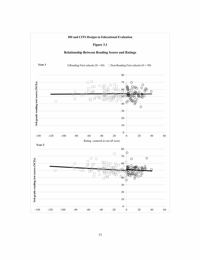
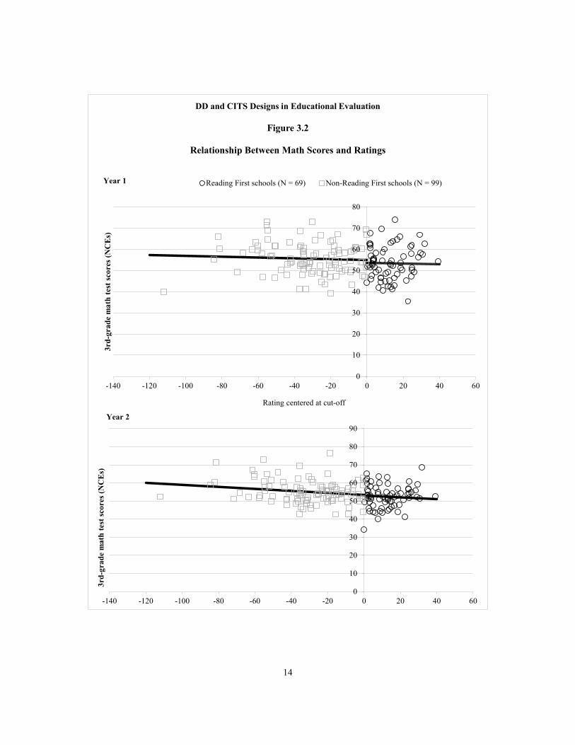
Figures 3.1 and 3.2 demonstrate how the RD design can be used to estimate the impact of Reading First on reading score and math scores, respectively. These figures plot the relationship between schools’ score on their application for Reading First funds (the rating variable) and the average third-grade test scores of their students during a given follow-up year (the outcome of interest). The ratings in these figures have been centered at the cut-off score, so the cut-off is located at zero. Schools above the cut-off received Reading First funds, while schools below the cut-off did not. The RD design assumes that, in the absence of the program, the relationship between the assignment variable and test scores would be continuous. Therefore, if the program is effective, it will create a discontinuity in the relationship between the assignment variable and the outcome at the cut-off point. The size of this discontinuity — or
16The members of this panel had advanced degrees and were knowledgeable in scientifically based reading research and the importance of explicit, systematic instructional strategies in phonemic awareness, phonics, fluency, vocabulary development, and comprehension. They also had collective expertise in professional development, leadership, assessment, curriculum, and teacher education. Reviewers worked in three-member teams that reviewed and scored each application.
17Ratings were based on the following nine criteria: (1) the program has been carefully reviewed; (2) the five components of reading instruction incorporate the five critical building blocks of effective reading instruction (phonemic awareness, decoding/word attack, reading fluency, vocabulary, and comprehension). (3) the program is based on sound principles of instructional design; (4) the program is valid and reliable; (5) the program employs a coherent instructional design; (6) content is organized around big ideas; (7) instructional materials contain explicit strategies; (8) instructional materials provide opportunities for teachers to scaffold instruction; (9) skills and concepts are intentionally and strategically integrated.
13
0
10
20
30
40
50
60
70
80
-140 -120 -100 -80 -60 -40 -20 0 20 40 60
3rd-
grad
e re
adin
g te
st sc
ores
(NC
Es)
Rating centered at cut-off score
DD and CITS Designs in Educational Evaluation
Figure 3.1
Relationship Between Reading Scores and Ratings
Reading First schools (N = 69) Non-Reading First schools (N = 99)Year 1
0
10
20
30
40
50
60
70
80
-140 -120 -100 -80 -60 -40 -20 0 20 40 60
3rd-
grad
e re
adin
g te
st sc
ores
(NC
Es)
Year 2
14
0
10
20
30
40
50
60
70
80
-140 -120 -100 -80 -60 -40 -20 0 20 40 60
3rd-
grad
e m
ath
test
scor
es (N
CEs
)
Rating centered at cut-off
DD and CITS Designs in Educational Evaluation
Figure 3.2
Relationship Between Math Scores and Ratings
Reading First schools (N = 69) Non-Reading First schools (N = 99)Year 1
0
10
20
30
40
50
60
70
80
90
-140 -120 -100 -80 -60 -40 -20 0 20 40 60
3rd-
grad
e m
ath
test
scor
es (N
CEs
)
Year 2

15
the difference between treatment and comparison group outcomes at the cut-off — is the estimated impact of the program.18
Based on these figures, it does not appear as though Reading First improved test scores, because there is no appreciable discontinuity in scores at the cut-off. We can formally estimate the size of the impact estimate — and test whether it is statistically different from zero — by fitting the following model:
𝑌𝑗 = 𝜋0 + 𝜓0𝑇𝑅𝐸𝐴𝑇𝑗 + 𝜌0𝑅𝐴𝑇𝐼𝑁𝐺𝐶𝑗 + 𝜀𝑗
where:
𝒀𝒋𝒕 = Average third-grade test score (reading or math) for school j in the spring of a follow-up year t.
𝑻𝑹𝑬𝑨𝑻𝒋 = Dichotomous indicator for whether school j is a treatment school (= 1 if school received Reading First funds; 0 if a non-Reading First school with a rating)
𝑹𝑨𝑻𝑰𝑵𝑮𝑪𝒋 = Continuous variable for the rating assigned to schools’ application centered at the cut-off (= 0)
In this model, 𝜓0 represents the estimated impact of the intervention in the follow-up year of interest.
Table 3.1 presents the impact estimates from this model, scaled as effect sizes. Effect sizes are based on a standard deviation of 21.06, which by definition is the student-level standard deviation for scores in normal curve equivalents (NCEs).19 The findings confirm that Reading First did not improve reading or math achievement. All impact estimates are small in
18This application of the RD design represents a “sharp” RD design, because all schools complied with their treatment assignment (that is, all schools above the cut-off received funding, and none of the schools below the cut-off received funding). With a sharp RD design, the discontinuity at the cut-off is an estimate of the treatment on the treated (TOT). In contrast, a “fuzzy” RD design is one where there is noncompliance (no-shows and crossovers). In this situation, the discontinuity at the cut-off is an estimate of the “intent to treat” (ITT).
19We use the student-level standard deviation because Reading First aims to improve student achievement. Normal curve equivalents are defined as 50 + 21.06z, where z is the z-score for a student’s score on the test. A standard deviation of 21.06 is used for scaling the test scores because this has the following result (assuming test scores are normally distributed): the NCE is 99 if the percentile rank of the raw score is 99; the NCE is 50 if the percentile rank of the raw score is 50; the NCE is 1 if the percentile rank of the raw score is 1.
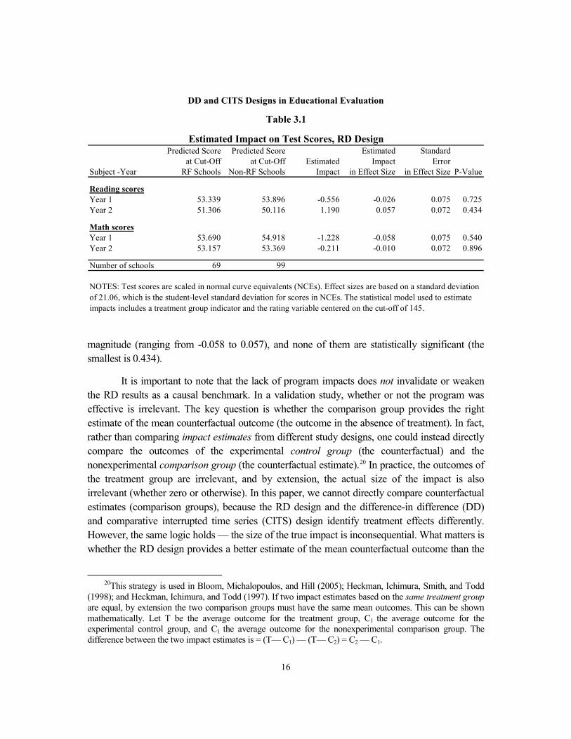
16
magnitude (ranging from -0.058 to 0.057), and none of them are statistically significant (the smallest is 0.434).
It is important to note that the lack of program impacts does not invalidate or weaken the RD results as a causal benchmark. In a validation study, whether or not the program was effective is irrelevant. The key question is whether the comparison group provides the right estimate of the mean counterfactual outcome (the outcome in the absence of treatment). In fact, rather than comparing impact estimates from different study designs, one could instead directly compare the outcomes of the experimental control group (the counterfactual) and the nonexperimental comparison group (the counterfactual estimate).20 In practice, the outcomes of the treatment group are irrelevant, and by extension, the actual size of the impact is also irrelevant (whether zero or otherwise). In this paper, we cannot directly compare counterfactual estimates (comparison groups), because the RD design and the difference-in difference (DD) and comparative interrupted time series (CITS) design identify treatment effects differently. However, the same logic holds — the size of the true impact is inconsequential. What matters is whether the RD design provides a better estimate of the mean counterfactual outcome than the
20This strategy is used in Bloom, Michalopoulos, and Hill (2005); Heckman, Ichimura, Smith, and Todd
(1998); and Heckman, Ichimura, and Todd (1997). If two impact estimates based on the same treatment group are equal, by extension the two comparison groups must have the same mean outcomes. This can be shown mathematically. Let T be the average outcome for the treatment group, C1 the average outcome for the experimental control group, and C1 the average outcome for the nonexperimental comparison group. The difference between the two impact estimates is = (T— C1) — (T— C2) = C2 — C1.
Predicted Score Predicted Score Estimated Standard at Cut-Off at Cut-Off Estimated Impact Error
Subject -Year RF Schools Non-RF Schools Impact in Effect Size in Effect Size P-Value
Reading scoresYear 1 53.339 53.896 -0.556 -0.026 0.075 0.725Year 2 51.306 50.116 1.190 0.057 0.072 0.434
Math scoresYear 1 53.690 54.918 -1.228 -0.058 0.075 0.540Year 2 53.157 53.369 -0.211 -0.010 0.072 0.896
Number of schools 69 99
Estimated Impact on Test Scores, RD Design
NOTES: Test scores are scaled in normal curve equivalents (NCEs). Effect sizes are based on a standard deviation of 21.06, which is the student-level standard deviation for scores in NCEs. The statistical model used to estimate impacts includes a treatment group indicator and the rating variable centered on the cut-off of 145.
Table 3.1
DD and CITS Designs in Educational Evaluation
17
other nonexperimental designs (NXD). Therefore, program effectiveness is not a necessary condition for a valid causal benchmark, but several other conditions do have to be satisfied, and we turn to them in the next section.
Specification Tests on the Causal Benchmark An RD impact estimate must meet three conditions to serve as a causal benchmark. It must be: (1) internally valid, (2) generalizable to all schools in the sample, and (3) sufficiently precise to provide an acceptable chance of detecting a nonzero impact if it exists.21 These three conditions — and the specification tests used to assess them in the context of Reading First — are discussed below. In summary, the results of these tests indicate that the RD impact estimates in Table 3.1 satisfy all three conditions and that estimated impacts from the RD design can be used as a benchmark to study the causal validity of the DD and CITS designs.
The RD Impact Estimates Must Be Internally Valid
The causal validity of an RD design hinges on four important conditions, which are discussed below.22 The test results are summarized below, with more detailed findings presented in Appendix A.
1) Nothing other than treatment status is discontinuous at the cut-point value of the RD rating (that is, there are no other relevant ways in which observations on one side of the cut-point are treated differently from those on the other side).
One way to test this condition is to estimate the “impact” of Reading First on variables that should not be affected by the program, such as the demographic characteristics of the student body and school-level test scores in the baseline period. The estimated impact of Reading First on these variables should be zero or not statistically significant. Accordingly, we examined the impact of Reading First on school characteristics that should be unaffected by the program, in the last baseline year, the first follow-up year, and the second follow-up year (See Appendix A). We find that Reading First did not have a statistically significant impact on these characteristics.
2) The rating variable cannot be caused by or influenced by the treatment. In other words, the rating variable is measured before the start of treatment or by a variable that can never change.
21Cook, Shadish, and Wong (2008) discuss the requirements for a strong within-study comparison of
experimental and nonexperimental estimates. We have adapted these requirements to using an RD design rather than an experimental design as the benchmark.
22See Bloom (2012) and Jacob, Zhu, Somers, and Bloom (2012) for a more detailed discussion.
18
As discussed earlier, ratings were assigned by an independent panel of experts based on a standard set of criteria, and therefore there was no opportunity to manipulate the ratings. Our qualitative review of the scoring materials and the rating process has convinced us that the ratings were indeed based on the scoring rubrics. Ratings were assigned before Reading First funds were awarded and could not have been influenced by the treatment or by political manipulation. Therefore, possible threats to validity leading to underestimates of program impacts — for example, that schools that received funds were somehow more disadvantaged, or that there was manipulation of ratings around the cut-off — are not plausible given the way in which the ratings were determined and funds were allocated.
McCrary (2008) also proposes a formal test of whether the ratings were “manipulated.” This test examines whether the distribution of the ratings is “disrupted” at the cut-off value, which would suggest that some schools’ rating scores were artificially raised so that they could just make the cut-off and get funding. The test is conducted by first creating a histogram of the density of the ratings, and then using a local linear regression on either side of the cut-off to estimate the discontinuity in the ratings density at the cut-off. Based on this test we do not find any evidence of manipulation.23
3) The cut-point is determined independently of the rating variable (that is, it is exogenous), and assignment to treatment is based entirely on the candidate ratings and the cut-point.
The cut-point is exogenous because it is based on the amount of available funding. After ratings were assigned, schools that applied for Reading First were ranked from highest to lowest based on their rating, along with the amount of funding requested (which was based on the size of the school). Funding was awarded to the highest-rated schools in rank order, until the available pool of funds was exhausted. Based on this funding algorithm, the 74 schools with the highest rating were awarded Reading First funding.24 The cut-off is equal to the rating at which funds were exhausted. (The cut-point between the lowest-scoring winning school and the highest-scoring losing school is 145.)
23The size of the discontinuity in the distribution of ratings at the cut-off is 0.736 (in logs), with a standard
error of 0.516. To run the test, one must choose a bin size for the histogram and a bandwidth for the local regression. McCrary proposes values based on a “rule of thumb,” but he stresses that these are only starting points, and that a more formal procedure should be used to determine the optimal bandwidth especially. Accordingly, we use the optimal bandwidth described in Imbens and Kalyanaraman (2009), which is 10 points on the rating scale; for the bin size, we use the default value proposed by McCrary (4.3 points).
24Although 74 schools received funding, 69 are used in the analysis because 5 schools do not have test score data for all baseline years. Using the RD design, estimated impacts for the 69 schools used in the analysis do not differ appreciably from impacts based on all 74 schools.

19
4) The functional form representing the relationship between the rating variable and the outcome is continuous throughout the analysis interval absent the treatment, and is specified correctly.
To estimate the impact of Reading First on student achievement, we use a simple linear RD model. We are confident that this is the correct functional form for several reasons. First, graphical inspection of the relationship between ratings and test scores clearly shows that it is linear and flat (Figures 3.1 and 3.2). Second, as a sensitivity test, we estimated impacts based on alternate function forms — allowing the relationship between the rating and test scores to be quadratic and cubic (see Appendix A). Impact estimates based on these alternate forms are not statistically significant and are similar in magnitude to the results based on a simple linear functional form.
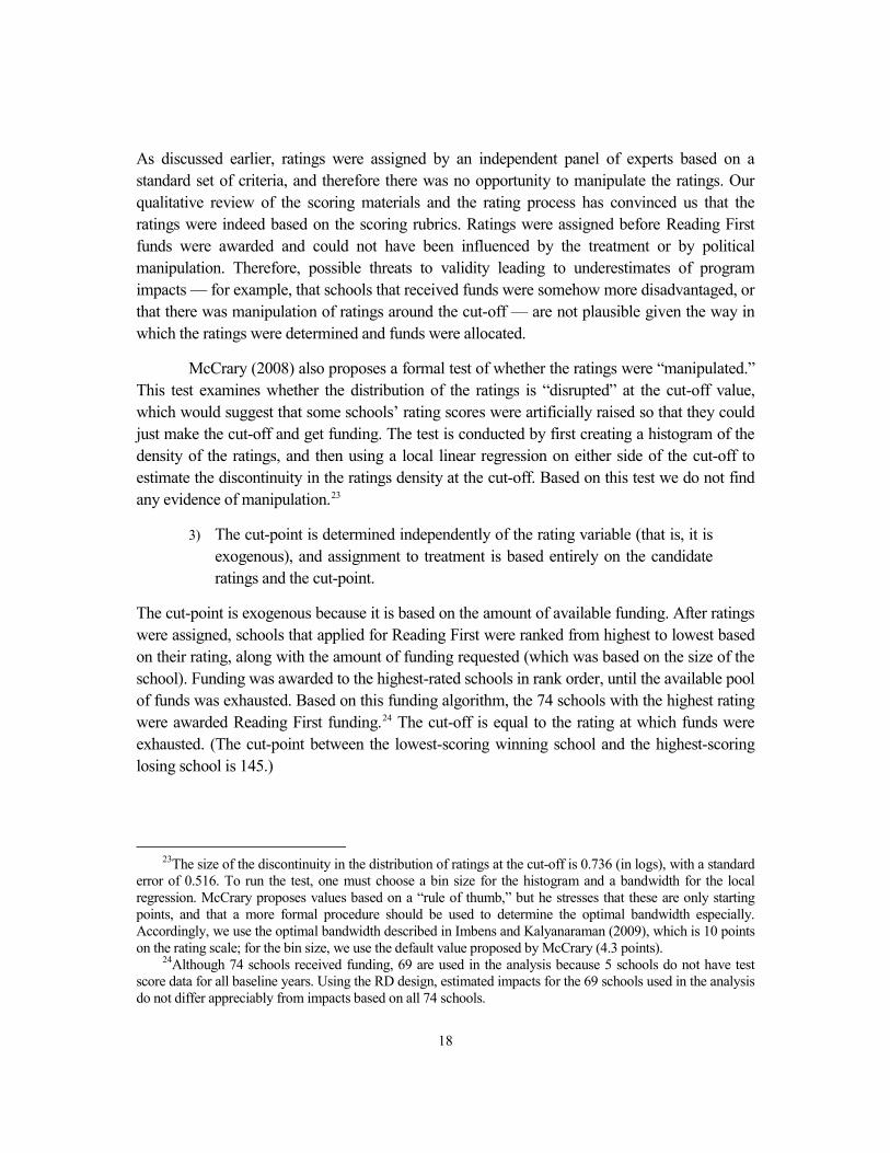
As a further specification test, the literature also recommends that impacts be estimated using only the subset of observations around the cut-off. The relationship between the rating variable and test scores is more likely to be linear around the cut-off, so impact estimates based on observations in this area are more likely to be correct. Accordingly, Figures 3.3 and 3.4 present RD impact estimates for different bandwidths h around the cut-off, for impacts on reading and math test scores, respectively. For all bandwidths — even those closest to the cut-off, where the functional form is most likely to be linear — we see that the estimated impact of Reading First hovers around zero and is not statistically significant.
In summary, these sensitivity analyses indicate that the RD estimate meets all four conditions for its internally validity and that the estimated impact of Reading First is not statistically significant and is zero for all practical purposes.
The RD Impact Estimates Must Be Generalizable to All Reading First Schools
In addition to being causally valid, the RD design must measure the same causal quantity as the DD and CITS designs to which it will be compared. In an RD, the mean counterfactual outcome for the treatment group is represented by the predicted outcomes of the comparison group at the cut-off point. Therefore, strictly speaking, RD impact estimates represent the effect of the program for participants around the cut-off only (the “local” average treatment effect). In contrast, the DD and CITS designs provide an estimate of the average impact for all Reading First schools (the average treatment effect).
Therefore, in order to use the RD as a benchmark, we must demonstrate that the RD estimates are generalizable to all schools. And specifically, we need to show that the Reading First had a “zero” impact not only for schools around the cut-off, but also for schools further

-0.5-0.4-0.3-0.2-0.1
00.10.20.30.40.5
10 15 20 25 30 35 40 45 50 55 60 65 70 75 80 85 90 95 100 105 110
Impa
ct e
stim
ate
(in e
ffec
t siz
e)
Bandwidth around cut-off (for rating variable)
DD and CITS Designs in Educational Evaluation
Figure 3.3
RD Impact Estimate on Reading Scores (and 95% CI) by Bandwidth Around Cut-Off
-0.5-0.4-0.3-0.2-0.1
00.10.20.30.40.5
10 15 20 25 30 35 40 45 50 55 60 65 70 75 80 85 90 95 100 105 110
Impa
ct e
stim
ate
(in e
ffec
t siz
e)
Year 1
Year 2
20
-0.5-0.4-0.3-0.2-0.1
00.10.20.30.40.5
10 15 20 25 30 35 40 45 50 55 60 65 70 75 80 85 90 95 100 105 110
Impa
ct e
stim
ate
(in e
ffec
t siz
e)
Bandwidth around cut-off (for rating variable)
DD and CITS Designs in Educational Evaluation
Figure 3.4
RD Impact Estimate on Math Scores (and 95% CI), by Bandwidth Around Cut-Off
-0.5-0.4-0.3-0.2-0.1
00.10.20.30.40.5
10 15 20 25 30 35 40 45 50 55 60 65 70 75 80 85 90 95 100 105 110
Impa
ct e
stim
ate
(in e
ffec
t siz
e)
Year 1
Year 2
21
22
away from the cut-off. We use three specification tests to assess whether impacts are heterogeneous across Reading First schools.
The first test compares the slopes of test scores against ratings on either side of the cut-off. If Reading First had somehow had an impact on Reading First schools further from the cut-off, an increase in these schools’ test scores would make the slope for Reading First schools different (steeper) than the slope for non-Reading First schools. As seen in Figures 3.1 and 3.2, however, the slope of the relationship between ratings and school-level test scores is the same on either side of the cut-off (and, in fact, it is flat). A statistical test confirms that the difference between slopes is not statistically significant (see Appendix A). This indicates that Reading First did not affect the test scores of schools further away from the cut-off any more than the test scores of schools closer to the cut-off.
The second way to examine whether effects are heterogeneous is to look at whether the estimated impact for all schools differs from the impact for schools around the cut-off. As shown in Figures 3.3 and 3.4, the estimated impact is the same (“zero”) for both groups of schools. The estimated impact of Reading First is stable across different subsamples of schools, which provides further evidence that the program did not improve the test scores of any particular subgroup of schools.
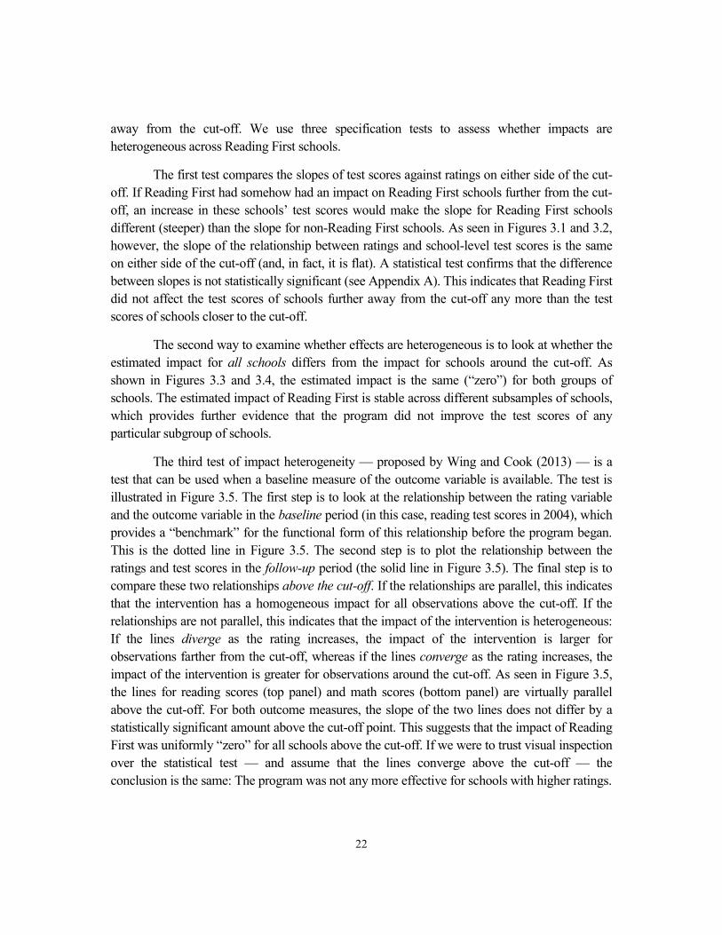
The third test of impact heterogeneity — proposed by Wing and Cook (2013) — is a test that can be used when a baseline measure of the outcome variable is available. The test is illustrated in Figure 3.5. The first step is to look at the relationship between the rating variable and the outcome variable in the baseline period (in this case, reading test scores in 2004), which provides a “benchmark” for the functional form of this relationship before the program began. This is the dotted line in Figure 3.5. The second step is to plot the relationship between the ratings and test scores in the follow-up period (the solid line in Figure 3.5). The final step is to compare these two relationships above the cut-off. If the relationships are parallel, this indicates that the intervention has a homogeneous impact for all observations above the cut-off. If the relationships are not parallel, this indicates that the impact of the intervention is heterogeneous: If the lines diverge as the rating increases, the impact of the intervention is larger for observations farther from the cut-off, whereas if the lines converge as the rating increases, the impact of the intervention is greater for observations around the cut-off. As seen in Figure 3.5, the lines for reading scores (top panel) and math scores (bottom panel) are virtually parallel above the cut-off. For both outcome measures, the slope of the two lines does not differ by a statistically significant amount above the cut-off point. This suggests that the impact of Reading First was uniformly “zero” for all schools above the cut-off. If we were to trust visual inspection over the statistical test — and assume that the lines converge above the cut-off — the conclusion is the same: The program was not any more effective for schools with higher ratings.
23
0
10
20
30
40
50
60
70
80
-140 -120 -100 -80 -60 -40 -20 0 20 40 60
3rd-
grad
e re
adin
g te
st sc
ores
(NC
Es)
Rating centered at cut-off score
DD and CITS Designs in Educational Evaluation
Figure 3.5
Relationship Between Reading Scores and Ratings, Baseline vs. Year 1
Year 1 test scores Baseline test scores (year 0)
Reading scores
0
10
20
30
40
50
60
70
80
-140 -120 -100 -80 -60 -40 -20 0 20 40 60
3rd-
grad
e m
ath
test
scor
es (N
CEs
)
Math scores
24
In conclusion, the findings from these specification tests strongly suggest that the “zero” impact of Reading First can be generalized to all schools in the sample. The most convincing piece of evidence in support of this claim is the fact that the relationship between ratings and test scores is almost perfectly horizontal. Because there is no relationship between the ratings and test scores, it seems highly implausible that there would be a relationship between the ratings and the magnitude of the impacts. Therefore, the estimated impact from the RD design represents the average treatment effect of Reading First, which is the same causal quantity that will be obtained from the DD and CITS designs.
The RD Impact Estimates Must Be Sufficiently Precise to Detect Policy-Relevant Impacts
As demonstrated elsewhere, estimates from the RD design have less statistical precision than other study designs (Bloom, 2012; Schochet, 2008).25 In practice, the standard error of impact estimates is two to four times greater for an RD design than for a randomized experiment with the same sample size. This is because there is a high correlation between the rating variable (RATING) and treatment status (TREAT) on the right-hand side of the RD model, which increases the standard error of the impact estimate.
By extension, a potential concern for this study is that Reading First may have improved test scores by a policy-relevant amount, but that these effects are not being detected because the precision of the estimated impact from the RD design is too low. We argue, however, that the statistical precision of the RD findings presented earlier is sufficient to make reliable conclusions, for two reasons.
First, the minimum detectable impact for the RD analysis in this paper is sufficiently small to be policy-relevant. Based on the standard errors reported in Table 3.1, the minimum detectable effect size (MDES) — or the smallest true impact that can be detected with 80 percent power and an alpha level of 5 percent — ranges from 0.20 to 0.21.26 We argue that this level of precision is acceptable, because smaller true impacts would not be policy-relevant; this is also the level of precision in many (if not most) school-level random assignment studies.
Second, we are confident that the true impact of Reading First is zero and that our conclusion that the program did not improve test scores is correct. To verify this proposition, we conducted a simple exercise. As shown in Figure 3.1, there is virtually no relationship between the ratings and reading test scores (the slope is horizontal). Therefore, in theory it is not
25See Appendix B for further details on the minimum detectable effect size for the RD design, as well as
the DD and CITS designs. 26The MDES is equal to 2.8 times the standard error in effect size.
25
necessary to control for the rating variable in the RD analysis, in which case the RD analysis model reduces to the model for a randomized experiment:
𝑌𝑗 = 𝜋0 + 𝜓0𝑇𝑅𝐸𝐴𝑇𝑗 + 𝜀𝑗
Based on this model, we find that the estimated impact on reading scores in the first year of Reading First (in effect size) is -0.015 and that this estimated impact is still not statistically significant at the 5 percent level, even though the precision of this analysis is much greater than the RD analysis. (The MDES for the “experimental” analysis is 0.14). This further supports our claim that conclusions from the RD design are not simply due to a lack of statistical power.


27
Section 4
The Difference-in-Difference Design and the Comparative Interrupted Time Series Design: Analytical Framework
Having established that the regression discontinuity (RD) design provides a reliable causal benchmark for the true impact of Reading First, we now turn to the two nonexperimental designs that are the focus of this paper: the comparative interrupted time series (CITS) design and the difference-in-difference (DD) design. As explained earlier, these two designs represent a trade-off between rigor and data requirements. The CITS design is more rigorous but requires more years of baseline data (four or more), while the DD design — which can be seen as a “simplification” of the CITS design — requires fewer years of baseline data, but its impact estimates are potentially more biased. The key question here is whether a DD design can produce internally valid estimates, in the event that sufficient data are not available for using a CITS design.
In this section, we begin by discussing how these two designs can be used to evaluate the impact of a school-level intervention such as Reading First. We then describe the comparison schools for these two designs — the process and methods used for selecting them and their characteristics relative to Reading First schools.
Overview of the DD and CITS Designs As noted earlier, the DD design evaluates the impact of a program by looking at whether — relative to the pre-intervention period — the treatment group makes greater subsequent gains than does the comparison group on the outcome of interest. This design has been used to evaluate a wide range of school-level education reforms, including the Talent Development program (Herlihy and Kemple, 2004; Kemple, Herlihy, and Smith, 2005), Project GRAD (Snipes, Holton, Doolittle, and Sztejnberg, 2006), and the First Things First program (Quint, Bloom, Black, and Stephens, 2005).
Figure 4.1 demonstrates the DD design using the example of Reading First, based on hypothetical data. Here we assume that third-grade reading scores are available for three baseline years and two follow-up years. To estimate program impacts, the first step is to determine the amount by which school’s average test scores change from baseline to follow-up (“change from baseline mean”). This change over time is estimated for both the treatment group (Reading First schools) and for comparison schools, for each follow-up year. The estimated impact of the program is then obtained as the change over time in the Reading First schools minus the change over time in the comparison schools. Mathematically, this is equivalent to

0
10
20
30
40
50
60
70
2002 2003 2004 2005 2006
Stat
e te
st sc
ores
(3rd
-gra
de r
eadi
ng)
Baseline period
DD and CITS Designs in Educational Evaluation
Figure 4.1
Estimating the Impact of Reading First Using a Difference-in-Difference Design(Hypothetical Data)
RF schools baseline mean
Comparison schools baseline mean
Follow-up period
Reading First begins Fall 2004
Change from baseline mean (RF schools)
Change from baseline mean (comparison schools)
ESTIMATED IMPACT = Change (RF) - Change (comparison)
28
29
estimating the difference in reading scores between Reading First schools and comparison schools at follow-up, and then subtracting the difference between the two groups of schools at baseline. Thus, the design implicitly adjusts for any difference in baseline means between treatment and comparison schools.
The rigor of the DD design (and any nonexperimental design) hinges on whether its comparison group provides a valid estimate of the mean counterfactual outcome for the treatment group. In a DD design, the estimated counterfactual outcome is the comparison group’s change over time from its baseline mean. In other words, we must assume that in the absence of the intervention, the treatment group would have made the same average gains (or losses) as the comparison group.
An important (and credible) threat to this assumption is that treatment and comparison schools may have different “maturation” rates. In Figure 4.1, for example, the larger gains made by Reading First schools could actually be due to a preexisting difference in the growth rates of treatment and comparison schools (as opposed to the impact of Reading First). Unfortunately, with less than four years of pretest data, it is almost impossible to determine the extent to which differential growth rates are a threat to causal validity.
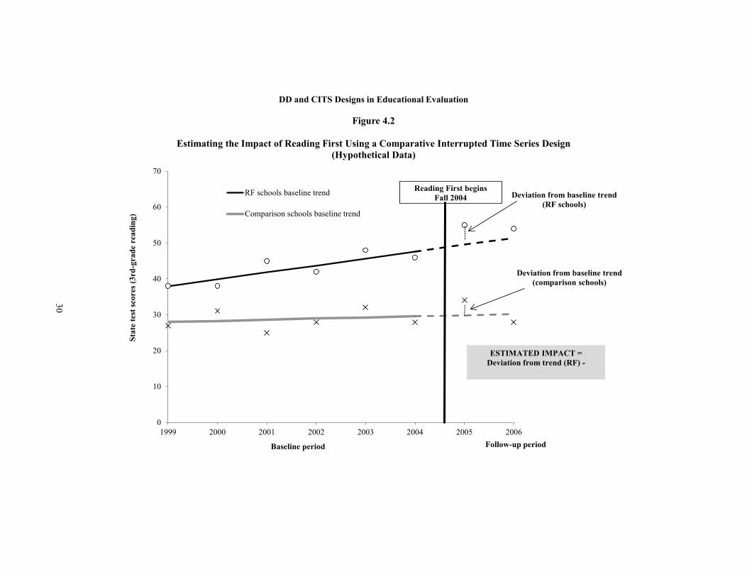
The CITS design addresses these concerns by making use of multiple years of pretest data. The impact of a program is evaluated by looking at whether — once the program begins — the treatment group deviates from its pre-intervention trend by a greater amount than does the comparison group. If so, the program is considered effective. The CITS design has more stringent data requirements than the DD design; in order to reliably estimate baseline trends, the CITS design requires pretest data for at least four time points before the intervention begins. For this reason, the CITS design has been less frequently used in program evaluation.27 However, due to the reporting requirements of No Child Left Behind, school-level test scores are now publicly available on a yearly basis, which makes the CITS design eminently feasible for evaluating school-level interventions. Bloom (2003) provides a general discussion of interrupted time series designs — with and without comparison groups — in the context of education research.
Figure 4.2 demonstrates, using hypothetical data, how the CITS design can be used to evaluate Reading First, assuming that six years of pretest data are available. (The reading scores for the last three baseline years are the same as in Figure 4.1.) The first step in a CITS design is to estimate the trend in third-grade test scores for each school during the baseline period. The second step is to estimate the amount by which schools’ test scores deviate from their baseline trend in the follow-up period (“deviations from baseline trend”). Average deviations from trend
27It has been used to evaluate the Jobs-Plus program (Bloom and Riccio, 2005), as well as No Child Left
Behind (Dee and Jacob, 2011; Wong, Cook, and Steiner, 2011).
0
10
20
30
40
50
60
70
1999 2000 2001 2002 2003 2004 2005 2006
Stat
e te
st sc
ores
(3rd
-gra
de r
eadi
ng)
Baseline period
DD and CITS Designs in Educational Evaluation
Figure 4.2
Estimating the Impact of Reading First Using a Comparative Interrupted Time Series Design (Hypothetical Data)
RF schools baseline trend
Comparison schools baseline trend
Reading First begins Fall 2004
Follow-up period
ESTIMATED IMPACT = Deviation from trend (RF) -
Deviation from baseline trend (RF schools)
Deviation from baseline trend (comparison schools)
30

31
are obtained for both Reading First schools and comparison schools. Finally, the impact of the intervention is estimated as the difference between the deviation from trend in treatment schools and the deviation from trend in comparison schools. If the program is effective, the deviation from trend for treatment schools will be greater than that for comparison schools.
The CITS design has greater potential than the DD design to provide valid inferences about program impacts, because it implicitly controls for differences between the “natural growth” rates of treatment and comparison schools. Figures 4.1 and 4.2 illustrate this point. In this hypothetical example, the DD design would incorrectly show that the program was effective. However, the CITS design would reveal that, in fact, the treatment and comparison schools are on different growth trajectories and that gains made by the treatment schools during the follow-up period are actually due to its higher pre-intervention growth rate and not to the effect of Reading First.
The CITS design is an especially rigorous study design for estimating longer-term impacts. By “longer term,” we mean impacts occurring in two to three years of follow-up, whereas “shorter-term” impacts are those in the first year of implementation. The ability to estimate longer-term impacts is important in educational evaluation, because it can take several years for an intervention to show visible effects on student achievement. Yet, longer-term impacts are harder to estimate because they are based on projections further into the future. Obtaining accurate projections is especially complicated when the slope of the baseline trend is not flat. The steeper the baseline slope, the less credible are projections further into the follow-up period, and by extension, the more questionable are estimates of longer-term impacts (since marked improvements for long periods of time are likely to be difficult to sustain).
Because the CITS design can account for baseline trends, it is better positioned than a DD design to estimate longer-term impacts, for two reasons. First, the CITS design can make more reasonable projections about longer-term outcomes and impacts because these projections are based on past trends. Second, the CITS design also provides a more realistic estimate of the precision of impact estimates: The standard error of the estimated impact increases for longer-term impacts, to account for the fact that projections into the follow-up period are less reliable as time goes by. In contrast, the DD design assumes that the reliability of projections is the same across follow-up periods, no matter how far into the future, and therefore the precision of DD estimates is the same regardless of the follow-up year. In education research, the assumption that longer-term projections are as reliable as short-term projections is unlikely to be correct, because the environment is unstable and constantly in flux. Therefore, the observed precision of DD impact estimates overestimates their true precision, especially for longer-term impacts. For

32
this reason, the CITS design provides a better reflection of the true precision of impact estimates than a DD design.28
All things considered, the rigor of a nonexperimental design can be viewed along a continuum defined by the number of years of available pretest data. With no pretest data at all, the validity of any NX impact estimate is not credible. With one to two years of baseline data, the causal validity of short-term impacts is questionable though credible. However, longer-term impacts should not be trusted because there is no known baseline trend from which to project outcomes far into the future. With three years of baseline data, the baseline mean is estimated with greater reliability and is less sensitive to policy shocks in any given year, which strengthens our ability to identify a credibly similar comparison group. Also, even though pre-intervention trends cannot be formally modeled, it becomes possible to gauge (at least descriptively) whether the treatment and comparison group have similar baseline slopes. In this context, the causal validity of short-term impacts is relatively sound, and longer-term impacts can be estimated, but only if baseline trends are quite flat (since projections into the future are more credible and reliable when outcomes are stable). With at least four years of baseline data, the validity of short-term impacts is strongest, because one can explicitly choose a comparison group with similar pre-intervention trends or statistically control for existing differences in baseline trends. Moreover, because baseline trends can be formally modeled, outcomes can be projected further into the future — and longer-term impacts can be estimated — even when the baseline slope is not flat. Having multiple years of pretest data also makes it possible to appropriately build additional uncertainty about future projections into the standard errors of long-term impact estimates (through estimates of the corresponding “standard errors of forecast”). Of course, there are limits to how far projections can be made. Even with many years of baseline data, impacts more than three years into the future should be viewed with extreme caution, because projections past this point become very unreliable
Though the CITS design is located at the favorable end of this continuum, it is not without limitations. In a CITS design, the comparison group’s deviation from its baseline trend provides an estimate of the mean counterfactual outcome for the treatment group. However, a potential threat to this assumption is that the treatment and comparison group are not subject to the same “policy events” occurring at the same time as the intervention being evaluated, such as another school reform initiative or massive staff turnover. If only one group of schools is subject to these additional events (whether treatment or comparison schools), the comparison group’s deviation from its trend will not provide the right counterfactual outcome for the treatment group, and the estimated impact of the program will be biased.29
28See Appendix B for technical details on the precision of CITS and DD designs. 29For example, one can imagine a situation in which Reading First schools simultaneously implemented
comprehensive school reform X in the follow-up period. This is a plausible scenario, because Reading First
33
That said, differential policy shocks are a threat to validity for both the DD and CITS designs. As argued by Cook and colleagues (2008), this threat can be mitigated by choosing comparison schools that are “local” and that have similar pretest scores. Strictly speaking, it is not necessary for the treatment and comparison groups to have similar pretest means, because the DD and CITS designs implicitly adjust for preexisting differences.30 Indeed, as mentioned earlier, previous validation studies have not taken the extra step of finding “matched” comparison schools for the DD design (for example, Fortson, Verbitsky-Savitz, Kopa, and Gleason, 2012). However, if schools have similar means and trends at baseline, this increases the likelihood that they will be subject to the same types of policy shocks (and have similar responses to them) in the follow-up period. In other words, the comparison group will have greater “credibility” or “face validity” as the source of counterfactual outcomes; hence the importance of strengthening the DD and CITS designs by carefully (and thoughtfully) selecting comparison schools. This process is discussed in the next section.
Selection of Comparison Groups One of the research questions of this paper is whether — in the context of the DD and CITS designs — some comparison group selections methods are superior to others with respect to bias reduction and/or precision gain. As noted elsewhere in this paper, there are many different strategies and methods for choosing comparison schools, some of which may provide a better representation of the mean counterfactual outcome than others (smaller bias). Similarly, some selection strategies yield larger comparison groups than others and, accordingly, will produce more precise impact estimates (greater precision). Therefore, in this paper we use several methods for selecting comparison groups, with the goal of comparing their bias reduction and precision gain.
Prescreened Groups
As argued by Cook, Shadish, and Wong (2008), comparison groups are more likely to provide the right counterfactual outcome when they are somehow “prescreened” for program participation. For example, members of a convincing comparison group should meet the geographical or needs-based conditions for participating in the intervention (prescreened for
schools might be more proactive about school improvement than other schools. In this situation, the comparison group’s deviation from trend or mean in the follow-up period will not accurately portray the deviation that Reading First schools would have experienced in the absence of the Reading First. Specifically, comparison schools did not implement either the comprehensive school reform or Reading First; therefore, a comparison of Reading First and comparison schools will provide an estimate of both Reading First and the other school reform, rather than just the effect of Reading First.
30The DD design implicitly controls for baseline differences in mean scores, while the CITS design also controls for any differences in baseline trends.

34
eligibility), or have taken the further step of submitting their name for consideration (prescreened for motivation). Narrowing the comparison pool based on ability, motivation, or some other known selection criterion is a way of simulating the selection process by which treatment schools came to be participants, which is important for producing a credible comparison group.
Accordingly, our first comparison group consists of schools that are located in districts eligible for Reading First funds. To be eligible, schools had to meet several criteria at both the district level and the school level. In terms of district-level requirements, a school had to be located in a Local Education Agency (LEA) that had at least one school with more than 50 percent of students reading below proficiency in fourth grade; a school’s LEA also had to fall within one of three prespecified categories for school improvement.31 In terms of the school-level eligibility requirements, schools themselves had to be among those in their district with the highest proportion of low-income students; have 50 percent or more students below “proficient” on the fourth-grade state reading assessment; and receive Title I funds.
Unfortunately, there are constraints on our ability to exactly identify eligible schools. We know which districts (LEAs) were eligible for Reading First, but we cannot identify exactly which schools within those districts were eligible. Therefore, our “eligible” group includes all schools in eligible districts — for a total 419 comparison schools spread across 79 eligible school districts — rather than eligible schools. The fact that we are unable to identify eligible schools may compromise this group’s credibility as a source of counterfactual outcomes, because the “eligible” group could include schools that were, in fact, not eligible to apply (or in other words, schools that are higher achieving than Reading First schools).
We use two strategies to create a more credible comparison group for Reading First schools. First, as an alternative comparison group, we use the 99 schools that applied for Reading First funds but did not receive them. By definition, these schools met all school-level and district-level eligibility criteria, but in addition, similar to the Reading First schools (the treatment group), they also had the motivation and resources to apply. These nonwinning applicants are the “non-RF group” in the RD design in Section 3.
As a second strategy for enhancing the credibility of the comparison groups, we use statistical matching methods to identify schools — among the “eligible” group — that are similar to the Reading First schools based on pretests and other school-level eligibility criteria
31The three categories are: (1) The LEA has jurisdiction over a geographic area that includes an area
designated as an empowerment zone (EZ) or an enterprise community (EC); (2) the LEA has jurisdiction over a significant number or percentage of schools that are identified for school improvement under section 1116(b) of Title I of the Elementary and Secondary Education Act (ESEA); or (3) the LEA has the highest number or percentage of children in the state who are counted by the U.S. Department of Education under section 1124(c) of Title I of the ESEA. In total, 103 districts in our midwestern state were eligible for Reading First funds.

35
(the percentage of low-income children and Title I status). In real-world applications, information on which schools applied for a program is not always known or relevant, so matching may be the only option for creating a credible comparison group. The creation of “matched” comparison sets is described in the next section.
Matched Groups
The creation of matched comparison groups entails three types of decisions. The first is the pool of candidates from which the comparison group is to be selected (comparison pool). The second is the set of characteristics on which to match schools (matching characteristics). The third is the statistical method used to select comparison schools (matching method). We created several comparison school sets based on different combinations of these factors, as described in greater detail below.
Comparison Pool
For the candidate pool for matching, we use the already defined group of 419 schools located in districts that are eligible to apply for Reading First funds. Matching is undertaken among the pool of schools in eligible districts (rather than among the 99 applicant schools), because some matching methods require a relatively large sample size; therefore, it is technically preferable to use the larger “eligible” pool as the group from which to select comparisons.
With respect to the matching exercise itself, Cook, Shadish, and Wong (2008) as well as others have emphasized the importance of using comparisons that are geographically local.32 In the case of Reading First, this would entail further restricting the comparison pool to schools in the same set of districts as the Reading First schools. In our study, taking this step would violate one of the conditions for a strong validation study. As discussed in Section 2, the RD design and the DD/CITS designs must provide impact estimates for the same target population, and therefore the comparability of the RD control group and the DD/CITS comparison groups is essential. If the candidate pool were restricted to schools in the same districts as the RF schools, all comparison schools (100 percent) used in the DD and CITS analysis would be located in districts that received Reading First funds, by definition. In contrast, only 59 percent of control schools in the RD design (those with a rating below the cut-off) are located in a district that received Reading First funds. As a result, if the comparison pool was strictly “local,” the RD and DD/CITS designs would be based on comparison groups with different compositions. However, by relaxing the requirement that comparison schools be “local,” the
32For example, see Heckman and Smith (1999); Heckman, Lalonde, and Smith (1999); and Heckman,
Ichimura, and Todd (1997).

36
comparison group for the DD/CITS designs will include schools in districts that did not receive Reading First funds, just like the RD control group.33
Although our inability to use a “local” comparison group is counter to conventional wisdom on “best practices,” it does afford an opportunity to examine whether using geographically local comparisons is a necessary condition for the causal validity of the DD and CITS designs. This is a relevant question in educational evaluation, because using comparisons in the same districts as the treatment schools may not always be feasible or appropriate. A pertinent example is when there is spillover of reform components to other schools within the district. In this situation, comparing treatment schools with other schools in their district would be biased downward, in which case it may be preferable to match the treatment schools to comparison schools located outside of the district. Although using comparison schools in the same districts is best where appropriate, it is also important to consider whether another option (that is, outside the district or a mix of within and outside as in the case of Reading First) might be more suitable, given the characteristics of the intervention.
Characteristics Used for Matching
The primary characteristic used for matching Reading First schools to comparison schools are the third-grade test scores of schools during the pre-intervention period. Pretests are strong predictors of outcomes in the follow-up period, so matching on school-level pretest scores (and where possible, their baseline trends) increases the credibility of comparison schools as a counterfactual for the treatment schools. For the analysis of impacts on reading achievement, we use reading test scores in the baseline period to identify “matched” comparison schools; similarly, for evaluating impacts on math achievement, we use math pretest scores to identify comparison schools.
In addition to pretests, we examine whether there is any benefit to also matching on other school characteristics like demographics. Specifically, we tried matching on test scores plus the following 12 school characteristics: the location of the school (rural or urban), total school enrollment, third-grade enrollment, the percentage of students who receive free or reduced price lunch, the racial/ethnic composition of the school (percentage of students who are white, black, Hispanic, Asian, or other), the percentage of third-grade students who are girls, the pupil-teacher ratio, and child poverty rates for the district. These characteristics were chosen because they have been used in the past to predict test scores. Matching on these characteristics may improve the comparability of the treatment and comparison schools and further reduce bias, because schools’ eligibility for Reading First funds was partly based on characteristics such as the percentage of low-income students.
33For example, among the comparison groups used in this analysis, the percentage of schools located in a district that did not receive Reading First funds ranges from 48 percent to 64 percent.
37
The number of years of baseline data used for matching depends on the design. For the CITS design, we use all six pre-intervention years of test scores and demographic data for matching (spring 1999 to 2004). For the DD design, we use the three most recent pre-intervention years (spring 2002 to 2004). Recall that the CITS design requires only four data points, and the DD design requires only one baseline point, so again we want to emphasize that our analysis represents a strong application of these two study designs. This is especially true for the DD design: As discussed earlier, using more baseline data points (and especially going from one data point to three data points) considerably strengthens the rigor of the analysis.
The next step in our analysis is to create a propensity score based on the matching characteristics. Because several characteristics and multiple years of data are used for matching, we need to collapse these variables into an overall index of “similarity” to make the process of matching more tractable. Several one-dimensional indices have been proposed — such as the Mahalanobis distance and the Euclidian distance — but in our analysis we use the propensity score method because it is the most common (Rosenbaum and Rubin, 1983).
The propensity score is calculated by fitting the following logistic regression model to a dataset that includes Reading First schools and schools in the “eligible” group (the candidate pool used for matching):34
𝑙𝑜𝑔𝑖𝑡�𝑇𝑅𝐸𝐴𝑇𝑗� = 𝛼 + � 𝛿𝑡𝑆𝐶𝑂𝑅𝐸𝑡2004
𝑡=𝑇0+ � � 𝛽𝑘𝑡𝑆𝑘𝑡
12
𝑘=1
2004
𝑡=𝑇0+ 𝜀𝑗
Where:
𝑻𝑹𝑬𝑨𝑻𝒋 = Dichotomous indicator for whether school j is a treatment school (= 1 if treatment school; 0 if a school in the comparison pool)
𝑺𝑪𝑶𝑹𝑬𝒕 = School-level test score in Year t (reading scores to create comparison groups for impacts on reading; math scores for impacts on math)
𝑺𝒌𝒕 = School characteristic S in Year t (12 characteristics) 𝜺𝒋 = Random error term for school j
34This regression is estimated on a “flattened” dataset — that is, with one observation per school. Time-
varying characteristics are expressed as multiple variables. For example, there is one test score variable per academic year (for example, READ1999, READ2000, etc.), and one value for each school characteristic per school year (for example, ENROLLMENT1999, ENROLLMENT2000, etc.).
38
The estimated coefficients from this logistic regression represent the relationship between school baseline test scores and characteristics and the log odds of being in the treatment group. They can be used to obtain the predicted probability that a school will be in the treatment group (that is, receive Reading First funds), given its characteristics. This predicted probability is defined as the propensity score. Viewed otherwise, the propensity score is simply a weighted composite of test scores and school characteristics, where the weight for a given characteristic is proportional to its ability to predict treatment status.35 Importantly, the difference between schools’ propensity scores provides a measure of their “dissimilarity.”
We estimate several sets of propensity scores for our analysis, based on different combinations of matching covariates and years of baseline data. For the CITS design, we use a propensity score based on all six years of pre-intervention data (t = 1999 to 2004). For the DD design, we use only three pre-intervention years of test scores and demographic data (t = 2002 to 2004). For each design, we estimate two sets of propensity scores: (a) one that includes test scores only and (b) one based on test scores and other baseline school characteristics.36 We also estimate separate propensity scores for math and reading. In total, we use eight sets of propensity scores, defined by number of year of baseline data (six or three), matching characteristic (test scores or test scores plus demographics), and subject matter (reading scores or math scores).
These propensity scores are then used as the metric for choosing comparison schools that are most “similar” to the Reading First schools. The algorithms (matching methods) used to select schools are described in the next section. In practice, we use the logit of the propensity score for matching, as recommended in the literature.37
35An alternative to matching on the propensity score is to match directly on schools’ baseline mean test
score and the slope of their baseline scores, using multidimensional matching. We conducted this analysis as a sensitivity check. The results from this analysis produce similar results (see Appendix F). However, the propensity score approach is easier to execute in practice, which is why it is the focus of our paper.
36Some schools do not have complete data on all of these school characteristics. We therefore impute these characteristics using a “dummy variable” approach (Allison, 2001). The missing value is imputed using a constant, and for each characteristic, we create a dichotomous indicator for whether a data point is imputed (= 1 if imputed, 0 otherwise). In the propensity score regression, we then include both the imputed characteristic and the missing data dichotomous indicator for that characteristic. In this way, “missingness” contributes to information determining probability of treatment assignment (Hansen, 2004).
37 The logit transformation is used for three reasons (Rubin, 2001). Because the logit transformation makes the propensity score linear, it is more relevant for assessing the results of linear modeling adjustments. Second, linear propensity scores tend to yield distributions with more similar variances and symmetry. Third, linear propensity scores are easier to relate to benchmarks in the literature on adjustments for covariates, which are based on linearity assumptions.

39
Matching Methods
As mentioned in the introduction, previous reviews have concluded that the statistical method used to select comparison schools matters little in terms of bias reduction. However, the choice of matching method does affect the number of comparison schools selected, and therefore the precision of impact estimates. In school-level impact evaluations — which typically have few units — maximizing the sample size may be an important consideration. Therefore, we create comparison school sets using matching methods that differ with respect to the number of comparison schools selected.38
The first selection method that we examine — and the one that is most popular in evaluation research — is nearest neighbor matching, also called “one-to-one” matching. This method chooses the most similar comparison school for each treatment school, based on the propensity score. Matching is conducted with replacement, which means that a given comparison school can be chosen as the “best” match for more than one treatment school. In this way, each treatment school is matched to the school that is most similar to it. The advantage of this type of matching is that it minimizes bias. Its disadvantage is that of all selection methods examined in this paper, it yields the smallest comparison group: Assuming that there are n treatment schools, there will be at most n unique comparison schools and perhaps far fewer than that, since a given comparison school can be matched to more than one treatment school.
For this reason, we also examine two selection approaches that yield larger comparison groups. These methods increase the sample size by “relaxing” some of the constraints imposed by using one-to-one matching with replacement. However, in doing so, these methods also introduce greater risk that impact estimates will be biased. Therefore, the question of interest is whether these alternative selection methods can increase the precision of impact estimates without compromising their causal validity.
The first alternative is to conduct one-to-one matching without replacement. In this variant of the nearest neighbor approach, a given comparison school can be matched to only one treatment school.39 Therefore, if there are n treatment schools, there will also be n unique comparison schools. When matching without replacement, two different approaches can be used. The first is to match each treatment school, one at a time, to its nearest neighbor among the remaining schools in the comparison pool at that point. There are several problems with this approach. The first is that a treatment school matched later in the process could end up with a poor match, which could reduce the overall balance between the treatment and comparison
38Methods not examined in this paper, for example, are kernel and local linear matching (Diaz and Handa, 2006) and full matching (Hansen, 2004).
39In contrast, one-to-one matching with replacement is sometimes called greedy nearest neighbor matching.

40
group. Second, the resulting comparison pool (and its quality) depends on the order in which treatment schools are matched. Therefore, when matching without replacement, a better approach is to use optimal nearest neighbor matching instead (Rosenbaum, 1989). When using an optimal algorithm, the goal is to find a comparison group of size n that minimizes the total distance between treatment and comparison schools, as opposed to the distance between each individual treatment-comparison pair. By this token, the optimal approach reduces the extent to which bias increases when comparison schools are selected without replacement. Moreover, with optimal matching, the order in which treatment schools are matched is irrelevant.40 This is the approach used in our analysis when matching without replacement.
The second alternative for increasing the size of the comparison group is to use radius matching, also known as “one-to-many” or “caliper” matching. In this approach, each treatment school is matched to all “suitable” comparison schools, defined as all schools within a given distance (or radius) of the treatment school as measured by the propensity score. Radius matching is conducted with replacement (a comparison school can be matched to more than one treatment school). The advantage of this method is that the size of the comparison group is larger than that for one-to-one matching; thus impact estimates are more precise. However, if the radius is too wide, greater precision will come at the cost of less “suitable” comparison schools, which could introduce bias into the impact estimate.
The challenge is finding the optimal radius — one that maximizes the sample size without compromising the validity of the comparison group as a source of estimates of the mean counterfactual outcome. Rough guidelines for the radius exist in the literature. Cochran and Rubin (1973) recommend a radius of 0.25 standard deviations (SD) on the propensity score as being sufficiently small to eliminate bias.
However, when pretest scores are available for two or more baseline years (as they are for the CITS design and in some cases the DD design), we propose that a more rigorous method can be used to determine the optimal radius.41 Specifically, we can choose the radius based on the program’s “impact” in the last baseline year. Because the intervention has not yet started at this point in time, we know that Reading First’s true impact in the last baseline year is zero, so we can use this as a benchmark for choosing the right radius. As the radius for matching expands, the estimate of this impact may deviate from zero because we are selecting “less similar” schools, but the precision of the impact estimate will increase as we include more schools in the comparison group. The goal is to choose the largest radius that still provides an estimated impact that does not differ statistically from zero.
40In contrast to the “optimal” algorithm, the first approach (where each treatment school is matched one at
a time) is sometimes referred to as a “greedy” matching algorithm. 41We are not aware of this method having been used in other studies.
41
We can use the mean squared error (MSE) as a metric for capturing the trade-off between bias and precision as the radius expands. The MSE for radius R is defined as follows:
𝑀𝑆𝐸�𝑅 = 𝜑𝑅�2 + 𝑣𝑎𝑟(𝜑𝑅� )
The first term, 𝜑𝑅�2 , is the square of the estimated impact in the last baseline year based
on a comparison group selected using radius R. Because the true impact in the last baseline year is zero, the first term 𝜑𝑅�
2 is also the squared bias of the estimated impact in the last baseline year.42 The second term measures the variance of the estimate. Assuming that there are multiple “good” matches for each comparison school, the MSE should initially decrease as the radius expands (since the variance will decrease without increasing bias). Then at some point, the MSE will start to increase as “bad” matches are chosen and bias is introduced into the estimates. Thus, the MSE is a useful measure for capturing the trade-off between bias and precision when selecting a radius.43
In practice, the optimal radius (and the final comparison group) can be determined by following these steps:
(1) The propensity score is calculated using pre-intervention data excluding the last baseline year (the latter being reserved for impact estimation in the next step);44
(2) Then for different values of radius R: a. Each Reading First school is matched to all comparison schools
within radius R, based on the propensity score from Step 1.45 b. The impact in the last baseline year (which should be zero) is then
estimated using the resulting comparison schools,46 and the MSE for radius R is calculated based on the estimated impact and its standard error.
(3) The “optimal” radius can then be determined — it is defined as the radius with the smallest MSE. In our analysis, the optimal radius ranges from 0.08
42The bias of 𝜑𝑅� is equal to 𝜑𝑅� minus the true impact of zero. 43In its most general form, the estimated MSE is defined as:
𝑀𝑆𝐸�𝜃�� = �𝜃� − 𝜃∗�2 + 𝑣𝑎𝑟(𝜃�) where 𝜃∗ is the true value of the parameter of interest and 𝜃�� is its estimate. 44This means that in this step, five baseline data points are used to estimate the propensity score for the
CITS design and two baseline data points are used for the DD design. 45For RF schools for which there is no match within radius R, we relax the criterion and simply select their
nearest neighbor, in order to ensure that all schools have a match. 46Impacts are estimated based on a variant of the CITS and DD models shown in Section 5.
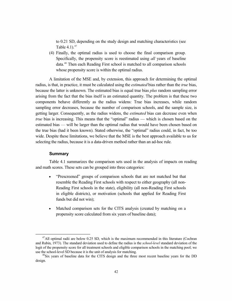
42
to 0.21 SD, depending on the study design and matching characteristics (see Table 4.1).47
(4) Finally, the optimal radius is used to choose the final comparison group. Specifically, the propensity score is reestimated using all years of baseline data.48 Then each Reading First school is matched to all comparison schools whose propensity score is within the optimal radius.
A limitation of the MSE and, by extension, this approach for determining the optimal radius, is that, in practice, it must be calculated using the estimated bias rather than the true bias, because the latter is unknown. The estimated bias is equal true bias plus random sampling error arising from the fact that the bias itself is an estimated quantity. The problem is that these two components behave differently as the radius widens: True bias increases, while random sampling error decreases, because the number of comparison schools, and the sample size, is getting larger. Consequently, as the radius widens, the estimated bias can decrease even when true bias is increasing. This means that the “optimal” radius — which is chosen based on the estimated bias — will be larger than the optimal radius that would have been chosen based on the true bias (had it been known). Stated otherwise, the “optimal” radius could, in fact, be too wide. Despite these limitations, we believe that the MSE is the best approach available to us for selecting the radius, because it is a data-driven method rather than an ad-hoc rule.
Summary
Table 4.1 summarizes the comparison sets used in the analysis of impacts on reading and math scores. These sets can be grouped into three categories:
• “Prescreened” groups of comparison schools that are not matched but that resemble the Reading First schools with respect to either geography (all non-Reading First schools in the state), eligibility (all non-Reading First schools in eligible districts), or motivation (schools that applied for Reading First funds but did not win);
• Matched comparison sets for the CITS analysis (created by matching on a propensity score calculated from six years of baseline data);
47All optimal radii are below 0.25 SD, which is the maximum recommended in this literature (Cochran
and Rubin, 1973). The standard deviation used to define the radius is the school-level standard deviation of the logit of the propensity score for all treatment schools and eligible comparison schools in the matching pool; we use the school-level SD because it is the unit of analysis for matching.
48Six years of baseline data for the CITS design and the three most recent baseline years for the DD design.

Definition of Group/ With MatchingComparison Set Name Selection Method Replacement? Characteristics Reading Math Reading Math Reading Math
Prescreened groupsState All non-RF schools in state -- -- -- -- 611 611 -- --
EligibleAll non-RF schools in eligible districts
-- -- -- -- 419 419 -- --
Applicants All non-RF schools that applied for funds
-- -- -- -- 99 99 -- --
Matched sets selected from "eligible" pool
For CITS design* Nearest neighbor Nearest neighbor Yes Baseline reading scores 1 1 62 59 -- -- NN w/out replacement Nearest neighbor (optimal) No Baseline reading scores 1 1 69 69 -- -- Radius Radius Yes Baseline reading scores 20 [1-41] 30 [1-50] 369 349 0.10 0.13 Radius w/ demographics Radius Yes Baseline scores +
demographics25 [1-66] 22 [1-68] 324 323 0.09 0.08
For DD design** Nearest neighbor Nearest neighbor Yes Baseline reading scores 1 1 58 65 -- -- NN w/out replacement Nearest neighbor (optimal) No Baseline reading scores 1 1 69 69 -- -- Radius Radius Yes Baseline reading scores 31 [1-54] 51 [2-86] 363 346 0.14 0.21 Radius w/ demographics Radius Yes Baseline scores +
demographics9 [1-23] 87 [1-164] 260 350 0.02 0.20
Number ofUniqueComparisonSchools
Number ofComparisonSchools perTreatment Schoola
OptimalRadius
Comparison School Sets
Table 4.1
DD and CITS Designs in Educational Evaluation
(continued)
43

* Matching is based on a propensity score calculated from 6 pre-intervention (baseline) years of data.** Matching is based on a propensity score calculated from 3 pre-intervention (baseline) years of data.
aMean (range).
Table 4.1 (continued)
NOTES: -- = Not applicable.
44

45
• Matched comparison sets for the DD analysis (created by matching on a propensity score calculated from three years of baseline data).
As explained earlier, matched comparison groups were chosen from the “eligible” pool based on different selection methods and matching characteristics to further improve the comparison schools as the source of mean counterfactual outcomes. The first matched group of schools is chosen based on the nearest neighbor method with replacement, the second using nearest neighbor matching without replacement (based on an optimizing algorithm), and the third using the radius method. All three sets are matched using a propensity score calculated from pretests only. The fourth comparison set uses radius matching, but matching is based on a propensity score calculated from pretests plus baseline demographics. Impact estimates based on the latter comparison group will be compared with those from the third group (radius matching based on pretests only) to examine whether also matching on demographic characteristics leads to greater bias reduction. We focus on radius matching for this comparison, because this method yields the largest sample and therefore the most reliable comparison of bias reduction.49
Two other issues are worth highlighting. First, among the “prescreened” groups, we include all non-Reading First schools in the state as a comparison group. This group is least likely to provide the correct counterfactual outcome, because some schools in the state were not even eligible for Reading First funds. However, we still include them as a comparison group in this paper, in order to examine the validity of the DD and CITS designs when no “prescreening” or matching is undertaken to improve the credibility of the comparison pool. Second, the CITS and DD comparison sets are matched using more years of baseline data than is typical for these designs (especially the DD design, which is often implemented with only one year of baseline data). Therefore, they represent especially strong applications of these designs.
Characteristics of the Comparison Groups Having chosen several viable comparison groups, the next step is to gauge their similarity to Reading First schools (the treatment group) before the start of the intervention, with respect to baseline test scores and demographic characteristics. As explained earlier, strictly speaking, the treatment and comparison group do not need to have similar baseline test scores before the intervention begins, because differences in test scores and slopes are controlled for by the analysis model. However, similar pretest scores — and if possible, similar demographic characteristics — do give greater credibility to the comparison group as the basis for estimating mean counterfactual outcomes in the follow-up period. For the purposes of this discussion, we will focus on the comparison groups used to estimate impacts on reading achievement, since the pattern of results for math is similar (see Appendix C).
49See Appendix C for tables showing the amount of overlap between schools in these sets.

46
Accordingly, Tables 4.2 to 4.4 present the characteristics of the comparison groups used in the reading analysis. In these tables, statistical tests of the difference between Reading First schools and other groups are not shown, for two reasons. First, the precision of the estimated difference varies across comparison groups. For a difference of given magnitude, comparison groups with more schools are more likely to be deemed statistically different from Reading First schools. Second, our goal is to assess the relative similarity of groups, so the statistical significance of differences is less relevant than the size of the observed differences and ultimately the size of the estimated bias. To this end, the tables present (in parentheses) the difference between Reading First schools and other groups as a standardized mean difference or effect size. These effect sizes are based on the school-level standard deviation for all schools in Reading First-eligible districts (69 Reading First schools plus the 419 non-Reading First schools in the eligible comparison pool) in the last baseline year.50 As a rule of thumb in propensity score matching, it has been suggested that treatment and comparison groups should differ by not more than 0.25 SD on key characteristics (Ho, Imai, King, and Stuart, 2007), so values greater than this threshold are flagged in the tables (“X”).
Table 4.2 presents the characteristics of the three prescreened comparison groups relative to the characteristics of Reading First schools (the treatment group). As expected, given the eligibility requirements, Reading First schools are much lower performing than other schools in the state (effect size difference = 0.70 for reading test scores in the last baseline year). Yet, Reading First schools are also lower performing than schools in districts that did meet the eligibility criteria (effect size difference = 0.53), which indicates that schools that were motivated to apply for Reading First funds had the lowest test scores among those eligible. For this reason, Reading First schools are most similar to the “applicant” group in terms of reading achievement — the effect size difference in pretest scores for this group is 0.05. On the other hand, Reading First schools and the “applicant” group are dissimilar with respect to demographic characteristics; effect size differences in racial/ethnic composition, enrollment, and poverty are larger than 0.25.
Tables 4.3 and 4.4 present the characteristics of the matched comparison groups chosen from the “eligible” group. We see that all matched comparison groups are reasonably similar to Reading First schools with respect to the baseline slope in test scores, as well as demographic characteristics. Importantly, effect size differences with respect to the propensity score are small
50See “Selection of Comparison Groups” earlier in this section for a discussion of the eligibility
requirements. We use the school-level standard deviation (rather than the student-level standard deviation), because in the matching literature, standardized mean differences are gauged based on the SD for the unit of observation (in this case schools). We use the standard deviation for all schools in eligible districts because it constitutes the largest relevant pool of schools. We use characteristics in the last baseline year because outcomes are not yet affected by the intervention at this point in time, and matching will be based on baseline characteristics.

47
RFSchool Characteristic Schools State Eligible Applicants
Baseline reading test scores
Predicted score in last baseline year 52.75 57.69 56.51 53.07(0.7) X (0.53) X (0.05)
Baseline trend (6 years) 1.24 1.26 1.28 1.23(0.01) (0.03) (-0.01)
Demographic characteristics (last baseline year)
Urban schools (%) 37.68 34.26 35.80 22.22(-0.07) (-0.04) (-0.32) X
Enrollment 382.61 409.56 400.13 362.55(0.17) (0.11) (-0.13)
Free/reduced-price lunch (%) 65.64 53.96 57.97 70.73(-0.56) X (-0.37) X (0.24)
Racial/ethnic composition (%) White 81.35 88.31 85.73 88.36
(0.37) X (0.23) (0.37) X Hispanic 2.50 1.60 1.68 1.35
(-0.24) (-0.22) (-0.31) X Black 15.17 9.16 11.54 9.70
(-0.37) X (-0.22) (-0.33) X Other 2.50 1.60 1.68 1.35
(-0.24) (-0.22) (-0.31) XNumber of 3rd-grade students 59.97 62.89 60.59 52.04
(0.1) (0.02) (-0.28) XFemale 3rd-graders (%) 47.91 47.48 47.56 46.69
(-0.09) (-0.08) (-0.26) XChildren in poverty in district (%) 22.00 20.66 22.45 25.75
(-0.19) (0.06) (0.54) XPupil-teacher ratio 14.47 15.57 15.40 14.32
(0.45) X (0.38) X (-0.06)
Number of schools 69 611 419 99
NOTES: Values shown in parentheses are the difference between RF and comparison schools in effect size. Effect sizes are calculated using the school-level standard deviation based on all schools in RF-eligible districts in the last baseline year (including both RF schools and non-RF schools). Differences greater than 0.25 SD are indicated with an "X." Statistical tests of the difference between Reading First schools and comparison schools are not shown, because the precision of the estimated difference varies across the comparison groups. (For a given effect size, larger comparison groups are more likely to be deemed statistically different from RF schools.)
Comparison Groups
Characteristics of Reading First Schools and Prescreened Comparison Groups (for Impacts on Reading Scores)
Table 4.2
DD and CITS Designs in Educational Evaluation

48
in magnitude, which indicates that the matching process has been properly executed. However, in terms of test score levels in the last baseline year, the comparability of the matched sets is more mixed. We note the following patterns across Tables 4.3 and 4.4:
• Selection methods (“nearest neighbor” versus “radius”). Among
matching methods, the nearest neighbor method produces the most similar comparison groups with respect to reading scores in the last baseline year. Effect size differences range from -0.004 to 0.11 when this method is used, which is on par with differences for the “applicant” group. In contrast, differences for the radius method range from 0.23 to 0.33. This pattern of results is to be expected, because the radius method selects several “suitable” matches for each Reading First school, as opposed to the nearest neighbor method which selects only the best match. Although pretest differences for the radius method are the largest among the matching methods, they are still much smaller in magnitude than test score differences for the “eligible” group from which they are drawn (effect size = 0.53, Table 4.2).
• Number of years of pre-intervention data (CITS sets versus DD sets.51) Matching on more years of pretest data (six years versus three years) decreases comparability with respect to test score levels in the last baseline year. This is especially apparent when the radius method is used: The difference in baseline test score levels is 0.33 SD when matching on six years of pretests, compared with 0.23 when matching on three years of pretests. This result suggests that matching on more information may actually put a constraint on one’s ability to match on pretest scores right before the intervention begins. However, one should remember that when using a CITS design, the most important consideration is that the treatment and comparison group should have similar baseline slopes, since this is the key element of the design for identifying impacts. As seen in Table 4.3, baseline slopes are indeed very similar when matching is conducted using six years of data (difference = -0.01 to -0.09), which confirms that matching for the CITS design was successful.
• Using demographic characteristics for matching (“radius” versus “radius with demographics”). Matching on demographics — in addition to pretest scores — does not appreciably improve the comparison group’s simi-
51CITS comparison sets are matched sets using six years of baseline data, while DD comparison sets are
matched using three years of data.
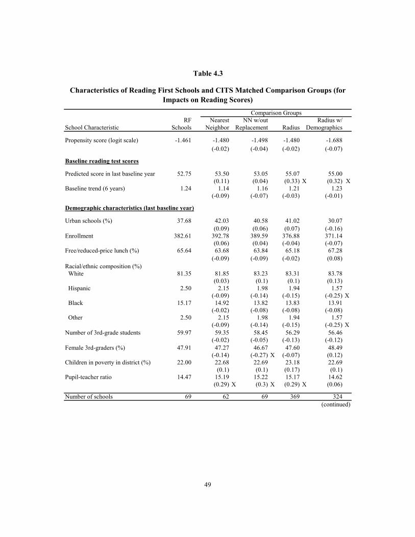
49
RF Nearest NN w/out Radius w/School Characteristic Schools Neighbor Replacement Radius Demographics
Propensity score (logit scale) -1.461 -1.480 -1.498 -1.480 -1.688(-0.02) (-0.04) (-0.02) (-0.07)
Baseline reading test scores
Predicted score in last baseline year 52.75 53.50 53.05 55.07 55.00(0.11) (0.04) (0.33) X (0.32) X
Baseline trend (6 years) 1.24 1.14 1.16 1.21 1.23(-0.09) (-0.07) (-0.03) (-0.01)
Demographic characteristics (last baseline year)
Urban schools (%) 37.68 42.03 40.58 41.02 30.07(0.09) (0.06) (0.07) (-0.16)
Enrollment 382.61 392.78 389.59 376.88 371.14(0.06) (0.04) (-0.04) (-0.07)
Free/reduced-price lunch (%) 65.64 63.68 63.84 65.18 67.28(-0.09) (-0.09) (-0.02) (0.08)
Racial/ethnic composition (%) White 81.35 81.85 83.23 83.31 83.78
(0.03) (0.1) (0.1) (0.13) Hispanic 2.50 2.15 1.98 1.94 1.57
(-0.09) (-0.14) (-0.15) (-0.25) X Black 15.17 14.92 13.82 13.83 13.91
(-0.02) (-0.08) (-0.08) (-0.08) Other 2.50 2.15 1.98 1.94 1.57
(-0.09) (-0.14) (-0.15) (-0.25) XNumber of 3rd-grade students 59.97 59.35 58.45 56.29 56.46
(-0.02) (-0.05) (-0.13) (-0.12)Female 3rd-graders (%) 47.91 47.27 46.67 47.60 48.49
(-0.14) (-0.27) X (-0.07) (0.12)Children in poverty in district (%) 22.00 22.68 22.69 23.18 22.69
(0.1) (0.1) (0.17) (0.1)Pupil-teacher ratio 14.47 15.19 15.22 15.17 14.62
(0.29) X (0.3) X (0.29) X (0.06)
Number of schools 69 62 69 369 324(continued)
Comparison Groups
Characteristics of Reading First Schools and CITS Matched Comparison Groups (for Impacts on Reading Scores)
Table 4.3

50
larity to Reading First schools, with respect to either demographics or pretest scores. In this case, matching only on pretest scores is sufficient for achieving comparability with respect to test scores and demographic characteristics, even though the latter are not included in the matching process. However, this might not always be true. Recall that in our analysis, a minimum of three years of baseline data are used for matching; the patterns we observe might not be generalizable to situations where only one or two years of pretest data are available.
In summary, the “applicant” and “nearest neighbor” groups have the greatest face validity, because they are most similar with respect to baseline test scores. Of the two, the “nearest neighbor” group is most credible, because it is also similar to the Reading First schools with respect to demographic characteristics.
NOTES: Values shown in parentheses are the difference between RF and comparison schools in effect size. Effect sizes are calculated using the school-level standard deviation based on all schools in RF-eligible districts in the last baseline year (including both RF schools and non-RF schools). Differences greater than 0.25 SD are indicated with an "X." Statistical tests of the difference between Reading First schools and comparison schools are not shown, because the precision of the estimated difference varies across the comparison groups. (For a given effect size, larger comparison groups are more likely to be deemed statistically different from RF schools.)
Table 4.3 (continued)
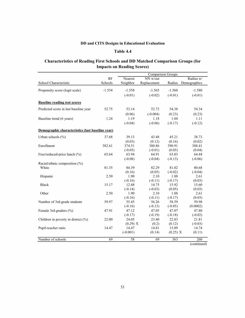
51
RF Nearest NN w/out Radius w/School Characteristic Schools Neighbor Replacement Radius Demographics
Propensity score (logit scale) -1.554 -1.558 -1.565 -1.560 -1.580(-0.01) (-0.02) (-0.01) (-0.01)
Baseline reading test scores
Predicted score in last baseline year 52.75 53.14 52.72 54.38 54.34(0.06) (-0.004) (0.23) (0.23)
Baseline trend (6 years) 1.24 1.19 1.18 1.04 1.11(-0.04) (-0.06) (-0.17) (-0.12)
Demographic characteristics (last baseline year)
Urban schools (%) 37.68 39.13 43.48 45.21 38.73(0.03) (0.12) (0.16) (0.02)
Enrollment 382.61 374.51 380.86 390.91 388.41(-0.05) (-0.01) (0.05) (0.04)
Free/reduced-price lunch (%) 65.64 63.94 64.91 63.03 64.44(-0.08) (-0.04) (-0.13) (-0.06)
Racial/ethnic composition (%) White 81.35 84.39 82.29 81.02 80.68
(0.16) (0.05) (-0.02) (-0.04) Hispanic 2.50 1.90 2.10 1.88 2.61
(-0.16) (-0.11) (-0.17) (0.03) Black 15.17 12.88 14.75 15.92 15.60
(-0.14) (-0.03) (0.05) (0.03) Other 2.50 1.90 2.10 1.88 2.61
(-0.16) (-0.11) (-0.17) (0.03)Number of 3rd-grade students 59.97 55.45 56.26 58.59 59.98
(-0.16) (-0.13) (-0.05) (0.0002)Female 3rd-graders (%) 47.91 47.12 47.05 47.07 47.80
(-0.17) (-0.19) (-0.18) (-0.02)Children in poverty in district (%) 22.00 24.05 23.40 22.83 21.81
(0.29) X (0.2) (0.12) (-0.03)Pupil-teacher ratio 14.47 14.47 14.81 15.09 14.74
(-0.001) (0.14) (0.25) X (0.11)
Number of schools 69 58 69 363 260(continued)
Comparison Groups
Characteristics of Reading First Schools and DD Matched Comparison Groups (for Impacts on Reading Scores)
Table 4.4
DD and CITS Designs in Educational Evaluation

52
NOTES: Values shown in parentheses are the difference between RF and comparison schools in effect size. Effect sizes are calculated using the school-level standard deviation based on all schools in RF-eligible districts in the last baseline year (including both RF schools and non-RF schools). Differences greater than 0.25 SD are indicated with an "X." Statistical tests of the difference between Reading First schools and comparison schools are not shown, because the precision of the estimated difference varies across the comparison groups. (For a given effect size, larger comparison groups are more likely to be deemed statistically different from RF schools.)
Table 4.4 (continued)
53
Section 5
Estimated Impacts from the DD and CITS Designs
In this section, we examine the estimated impact of Reading First based on the difference-in-difference (DD) and comparative interrupted time series (CITS) designs, for each of the comparison groups listed in Table 4.1. To examine the robustness of our conclusions, we replicate the analysis across two follow-up years (first and second year of the intervention) and two outcomes (reading scores and math scores). Before reviewing the findings, we first describe the statistical models used to estimate impacts as well as the criteria used to compare the impact estimates and to answer our research questions.
Statistical Models Used to Estimate Impacts The DD and CITS impacts are estimated using multilevel regression models to account for the fact that there are multiple test scores per school (one for each school year). As described elsewhere, it is important to account for such clustering; otherwise the standard errors of impact estimates will be too small (Bertrand, Duflo, and Mullainathan, 2002).
For the DD design, we fit a multilevel model to a panel (longitudinal) dataset that includes the test scores and school characteristics of the Reading First schools and the relevant comparison group, for three pre-intervention years and two follow-up years:
Level 1 (school years within schools):
𝑌𝑗𝑡 = 𝛼0𝑗 + 𝛽0𝑗𝑇𝑅𝐸𝐴𝑇𝑗 + 𝛼1𝑌𝑅1𝑡 + 𝛽1𝑇𝑅𝐸𝐴𝑇𝑗 ∗ 𝑌𝑅1𝑡 +𝛼2𝑌𝑅2𝑡 + 𝛽2𝑇𝑅𝐸𝐴𝑇𝑗 ∗ 𝑌𝑅2𝑡 + 𝜀𝑗𝑡
Level 2 (schools):
𝛼0𝑗 = 𝛼0 + 𝑢𝑗 where j denotes schools and time t spans three baseline years (2002-2004) and two follow-up years (2005 and 2006). The variables in the model are defined as follows:
𝒀𝒋𝒕 = Average third-grade test score (reading or math) for school j in spring of year t
𝑻𝑹𝑬𝑨𝑻𝒋 = Dichotomous indicator for whether school j is a treatment school (= 1

54
if school received Reading First funds; 0 if a comparison school)
𝒀𝑹𝟏𝒕 = Dichotomous indicator for test scores in the first intervention year (= 1 if 2005; 0 otherwise)
𝒀𝑹𝟐𝒕 = Dichotomous indicator for test scores in the second intervention year (= 1 if 2006; 0 otherwise)
𝒖𝒋 = Between-school random variation in the baseline mean
𝜺𝒋𝒕 = Random variation in test scores across time within schools (within-school variation) 52
From this model, we can obtain estimates of the following quantities of interest:
𝛼0 = Baseline mean for the comparison schools
𝛼0 + 𝛽0 = Baseline mean for the treatment schools
𝛼1 = Change over time from the baseline mean for the comparison schools in Year 1 of the intervention
𝛼1 + 𝛽1 = Change over time from the baseline mean for the treatment schools in Year 1 of the intervention
𝛼2 = Change over time from the baseline mean for the comparison schools in Year 2 of the intervention
𝛼2 + 𝛽2 = Change over time from the baseline mean for the treatment schools in Year 2 of the intervention
Therefore, the estimated impact of the intervention in Year 1 — the change over time for treatment schools minus the change over time for comparison schools — is 𝛽1. Similarly, the estimated impact in Year 2 is 𝛽2. The standard error of these coefficients (which accounts for clustering) can be used to test whether the estimated impact in each follow-up year is statistically different from zero. Impact analyses with comparison sets created with replacement and/or one-to-many matching are weighted.53
For the CITS design, we use the following multilevel model, which is fitted to data for all six baseline years and the two follow-up years:
52The covariance structure of this model — whereby time points are nested within schools — accounts for
the clustering of time points within schools. 53Analyses with the nearest neighbor comparison set (with replacement) use weights to account for the
number of times a comparison school is selected as a match. Analyses based on the radius method use weights to account for variation in the matching ratio across treatment schools as well as the number of times a comparison school is selected as a match.

55
Level 1 (school years within schools):
𝑌𝑗𝑡 = 𝛼0𝑗 + 𝛽0𝑗𝑇𝑅𝐸𝐴𝑇𝑗 + 𝜙0𝑗𝑅𝐸𝐿𝑌𝐸𝐴𝑅𝑡 + 𝜆0𝑅𝐸𝐿𝑌𝐸𝐴𝑅𝑡 ∗ 𝑇𝑅𝐸𝐴𝑇𝑗 +𝛼1𝑌𝑅1𝑡 + 𝛽1𝑇𝑅𝐸𝐴𝑇𝑗 ∗ 𝑌𝑅1𝑡 + 𝛼2𝑌𝑅2𝑡 + 𝛽2𝑇𝑅𝐸𝐴𝑇𝑗 ∗ 𝑌𝑅2𝑡 + 𝜀𝑗𝑡
Level 2 (schools):
𝛼0𝑗 = 𝛼0 + 𝑢𝑗
𝜙0𝑗 = 𝛽0 + 𝜏𝑗
where j denotes schools and time t spans all six baseline years (1999-2004) and two follow-up years (2005 and 2006). Variables are defined as before, with the addition of the following variables to measure the trend in test scores and the between-school variation in the baseline intercept and trend:
𝑅𝐸𝐿𝑌𝐸𝐴𝑅𝑡 = Continuous variable for time period (school year) centered at the last baseline year (= 0 in 2004).
𝑢𝑗 = Between-school random variation in the baseline intercept (centered at the last baseline year)
𝜏𝑗 = Between-school random variation in the baseline slope54
The model provides estimates of the following quantities:
𝛼0 = Baseline mean (intercept) for the comparison schools in the last
baseline year
𝛼0 + 𝛽0 = Baseline mean (intercept) for the treatment schools in the last baseline year
𝜙0 = Baseline slope for the comparison schools
𝜙0 + 𝜆0 = Baseline slope for the treatment schools
𝛼1 = Deviation from baseline trend for the comparison schools in Year 1 of the intervention
𝛼1 + 𝛽1 = Deviation from baseline trend for the treatment schools in Year 1 of the intervention
54Similar to the DD model, the covariance structure accounts for the nesting of time points (school years)
within schools, by allowing the baseline mean and slope to vary randomly across schools.
56
𝛼2 = Deviation from baseline trend for the comparison schools in Year 2 of the intervention
𝛼2 + 𝛽2 = Deviation from baseline trend for the treatment schools in Year 2 of the intervention
Thus, in this model, 𝛽1 represents the estimated impact in Year 1 — the deviation from trend for treatment schools minus the deviation from trend for comparison schools. Similarly, the estimated impact in Year 2 is 𝛽2. As in the DD design, one can then use the standard error of these coefficients to test whether the estimated impact is statistically different from zero. Impact analyses with comparison sets created with replacement and/or one-to-many matching are weighted.
Like the regression discontinuity (RD) findings presented in Section 3, all CITS and DD impact estimates and standard errors presented in this section are in effect sizes. Effect sizes for both reading and math are based on a standard deviation of 21.06, which is the student-level standard deviation for scores in normal curve equivalents (NCEs).55 More detailed results from the impact analysis — in their original scale — can be found in Appendix D.
Criteria for Comparing Impact Estimates: Bias and Precision One of the key questions in this paper is whether the CITS and DD designs can produce internally valid estimates of program impacts. To answer this question, we calculate the bias for each DD and CITS estimate, defined as the difference between the DD or CITS impact estimate and the RD impact estimate (the causal benchmark):
𝐵𝐼𝐴𝑆𝑁𝑋𝐷� = 𝐼𝑁𝑋𝐷�− 𝐼𝑅𝐷�
where 𝐼𝑅𝐷� is the estimated impact from the RD design and 𝐼𝑁𝑋𝐷� is the estimated impact from the DD or CITS design.
As seen here, the bias is assessed based on two impact estimates, each of which is estimated with error. Therefore, what we observe is in fact the estimated bias, which is also estimated with error. This error must be taken into account when interpreting the magnitude of the estimated bias, and, in particular, we must determine whether the confidence interval around each impact estimate includes zero. If it does, there is no evidence that the DD or CITS impact estimates are biased.
55We use the student-level standard deviation because Reading First aims to improve student achievement.
In contrast, the effect sizes in Tables 4.2 to 4.4 are based on the school-level standard deviation, because these tables examine the success of the matching exercise, which should be gauged based on school-level outcomes, since schools are the unit used for matching.
57
To conduct hypothesis testing on the estimated bias, we need to determine its standard error. Yet obtaining the correct standard error is tricky, because the impact estimates being compared (𝐼𝑅𝐷� and 𝐼𝑁𝑋𝐷�) are not independent: The treatment group is the same across impact estimates, and there is also overlap in the comparison groups used to estimate each impact.56 In order to make correct inferences about the size of the bias, the standard error of the estimated bias must account for this dependence. If we were to incorrectly assume that the impact estimates are independent, the standard error of the estimated bias would be too large, and we could mistakenly conclude that the estimated bias is not statistically significant, when in fact it is. We use nonparametric bootstrapping to obtain the right standard errors for the estimated bias. Bootstrapped standard errors account for the dependence between impact estimates and can be used to test whether the estimated bias for a given DD or CITS impact estimate is statistically different from zero.57 In addition, bootstrapping is also used to test whether bias estimates differ across different comparison group selection methods, as well as across the DD and CITS designs.58
Finally, we also compare the standard error of impact estimates, as a means of gauging their relative precision. Precision is especially relevant for the choice of the comparison group selection method. As noted earlier, some matching methods produce larger comparison groups, and therefore the resulting impact estimates are more precise. Assuming that two methods have similar bias, the method whose estimates are more precise is preferred because it increases the likelihood of detecting policy-relevant impacts.
Previous validation studies have opted for criteria other than bias and precision to compare impact estimates across designs, so it is incumbent on us to explain why we do not use them in our analysis. The first such criterion is the statistical significance of impact estimates — that is, whether inferences about program effectiveness (based on p-values) are the same across study designs.59 In our study, we do not use this criterion for two reasons. The first reason is conceptual. In a validation study, the key question is not whether the program is effective (as
56For example, some of the non-Reading First schools used in the RD analysis are also comparison
schools in the DD or CITS analyses. See Appendix C for tables showing the amount of overlap between comparison groups.
57Importantly, bootstrapping also accounts for uncertainty in the propensity score matching process. A bootstrapping approach is also used in Fortson, Verbitsky-Savitz, Kopa, and Gleason (2012). Appendix E provides further information on the bootstrapping process. Appendix E also presents estimates of the correlation between the RD and CITS/DD impact estimates, which confirms that they are indeed highly correlated to each other.
58Formally, we test whether the difference in bias estimates between two methods (for example, between nearest neighbor matching and radius matching or between DD and CITS) is statistically different from zero. If not, there is no evidence that the DD and CITS designs and/or different selection methods are differentially biased. Standard errors for these tests are also obtained using nonparametric bootstrapping. See Appendix E for details.
59This approach is used in Cook et al. (2008).

58
discussed in Section 3, the size of the impact is irrelevant), but whether impact estimates differ from each other. Accordingly, the relevant hypothesis test in a validation study is whether differences between impact estimates are statistically significant, not whether impact estimates themselves are statistically significant. The second reason for not using the statistical significance of individual impact estimates as a criterion is more technical. The impact estimates in our analysis differ in terms of their precision, due to differences in the study design and the size of the comparison group. When precision differs across two estimates, these estimates may exhibit different patterns of statistical significance, even when both of them are internally valid. In other words, bias and precision are confounded. As described earlier, we prefer to consider bias and precision separately, since bias is the most important consideration in a validation study.
Previous studies have also used the mean squared error (MSE) as a criterion for comparing impact estimates.60 This metric was discussed in Section 3, in the context of determining the optimal radius for the radius matching method.61 We do not use the MSE as a criterion for comparing impact estimates in this paper because it suffers from the same problem as statistical significance: By definition, it combines the bias and precision of an estimated impact into one measure, which makes it difficult to compare the MSE of different impacts estimates. We argue that it is more useful to consider bias and precision separately, as outlined in our approach.62
Impacts on Reading Scores As a visual guide for interpreting the CITS and DD impact estimates, Figures 5.1 and 5.2 plot the baseline and follow-up reading test scores (in NCEs) for Reading First schools and each of the comparison groups. As seen in these figures, the baseline slope in reading test scores for Reading First schools is relatively flat, meaning that test score growth was quite stable in the baseline period. We also see an abrupt drop in test scores in Year 2, perhaps due to a rescaling of reading test scores. These general patterns are also observed in the comparison groups, which gives credibility to these groups as valid reference points. The one exception — as already noted — are the “state” and “eligible” groups, whose reading test scores are substantially higher than those of Reading First schools and the other comparison groups (Figure 5.1). From these figures, we can also see that Reading First did not appreciably affect reading achievement —
60This approach is used in Orr, Bell, and Kornfeld (2004). 61The MSE for an impact estimate is equal to the square of the estimated bias, plus the variance of the
impact estimate. 62Bell and Orr (1995) also propose comparing impact estimates using a Bayesian “maximum risk
function.” However, we do not use it in our analysis, because it requires making a decision about a “policy-relevant” cut-off for the impact. This is difficult to determine in the case of impact on test scores.
59
test scores in Reading First schools did not improve by a greater amount in the follow-up period relative to the comparison schools.
Estimated Bias
Figures 5.3 and 5.4 present impact estimates and 95 percent confidence intervals for the CITS design and DD designs in the first and second year of the intervention, for each comparison group. These figures also include the “benchmark” RD impact estimate and its confidence interval, as a reference point.
In general, we see that all impact estimates (including the RD benchmark) hover around zero and that there is no discernible pattern of bias. There is also substantial overlap in the confidence intervals for the RD impact estimate and the intervals for other estimates, which suggests that the DD and CITS estimates are not statistically different from the causal benchmark. As noted earlier, however, the impact estimates are correlated, and so, strictly speaking, the confidence intervals cannot be directly compared.
Accordingly, Table 5.1 presents formal tests of whether estimated bias for each DD and CITS estimate is statistically significant. Recall that the estimated bias is defined as the difference between the DD or CITS estimate and the RD impact estimate, which here are scaled as an effect size. Bias estimates are small in magnitude, ranging from -0.11 to 0.04. Based on bootstrapped standard errors — which account for the correlation among impact estimates — none of these bias estimates come close to being statistically significant at the 5 percent level, for either study design (DD or CITS) or intervention year (Year 1 or Year 2). This confirms that all impact estimates are internally valid.
Differences in Bias and Precision Across Comparison Groups
Next, we can compare the size of the estimated bias and the precision of impact estimates across study designs, matching methods, and matching characteristics. Bias estimates for each group are presented in Table 5.1, while the standard error of each impact estimate is shown in Figures 5.3 and 5.4. Statistical tests for the difference in bias estimates across groups and designs (based on bootstrapping) can be found in Appendix E. The key findings are as follows:
• DD design versus CITS design: The two study designs are very similar with respect to their estimated bias and precision. For a given selection method, the estimated bias does not statistically differ across the two study designs. The two designs provide similar estimates because the baseline trend in test scores in similar for Reading First schools and comparison schools (as
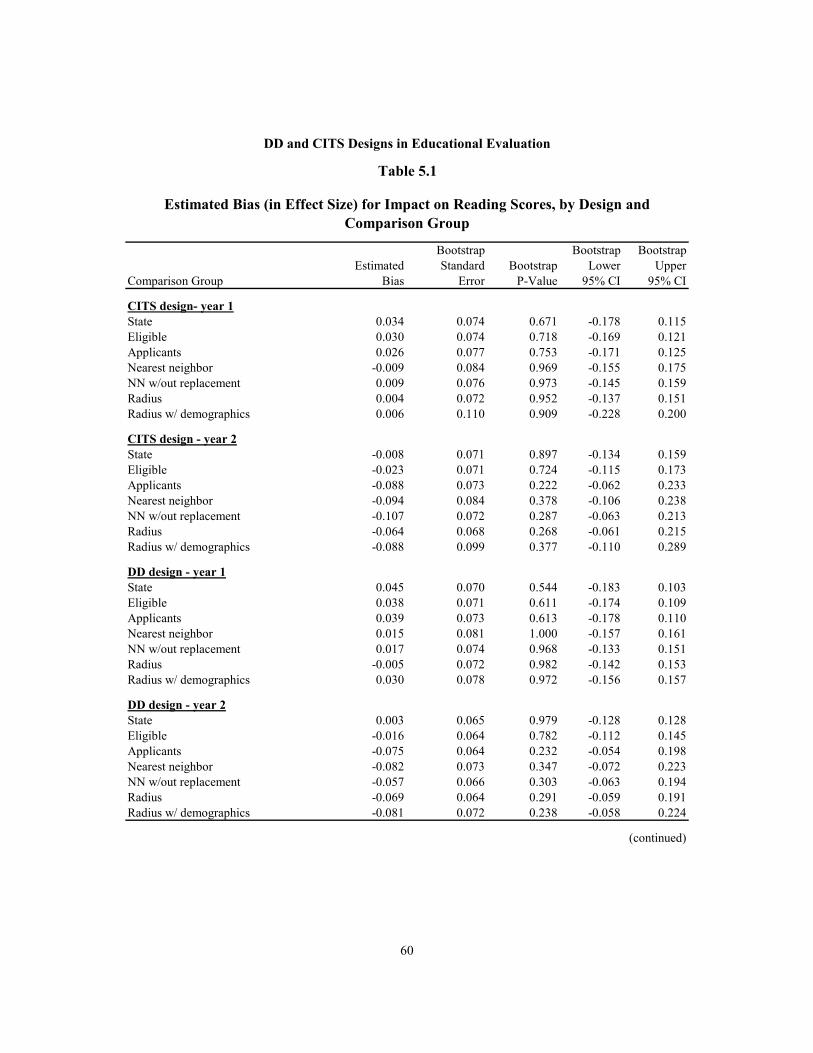
60
Bootstrap Bootstrap BootstrapEstimated Standard Bootstrap Lower Upper
Comparison Group Bias Error P-Value 95% CI 95% CI
CITS design- year 1State 0.034 0.074 0.671 -0.178 0.115Eligible 0.030 0.074 0.718 -0.169 0.121Applicants 0.026 0.077 0.753 -0.171 0.125Nearest neighbor -0.009 0.084 0.969 -0.155 0.175NN w/out replacement 0.009 0.076 0.973 -0.145 0.159Radius 0.004 0.072 0.952 -0.137 0.151Radius w/ demographics 0.006 0.110 0.909 -0.228 0.200
CITS design - year 2State -0.008 0.071 0.897 -0.134 0.159Eligible -0.023 0.071 0.724 -0.115 0.173Applicants -0.088 0.073 0.222 -0.062 0.233Nearest neighbor -0.094 0.084 0.378 -0.106 0.238NN w/out replacement -0.107 0.072 0.287 -0.063 0.213Radius -0.064 0.068 0.268 -0.061 0.215Radius w/ demographics -0.088 0.099 0.377 -0.110 0.289
DD design - year 1State 0.045 0.070 0.544 -0.183 0.103Eligible 0.038 0.071 0.611 -0.174 0.109Applicants 0.039 0.073 0.613 -0.178 0.110Nearest neighbor 0.015 0.081 1.000 -0.157 0.161NN w/out replacement 0.017 0.074 0.968 -0.133 0.151Radius -0.005 0.072 0.982 -0.142 0.153Radius w/ demographics 0.030 0.078 0.972 -0.156 0.157
DD design - year 2State 0.003 0.065 0.979 -0.128 0.128Eligible -0.016 0.064 0.782 -0.112 0.145Applicants -0.075 0.064 0.232 -0.054 0.198Nearest neighbor -0.082 0.073 0.347 -0.072 0.223NN w/out replacement -0.057 0.066 0.303 -0.063 0.194Radius -0.069 0.064 0.291 -0.059 0.191Radius w/ demographics -0.081 0.072 0.238 -0.058 0.224
(continued)
DD and CITS Designs in Educational Evaluation
Table 5.1
Estimated Bias (in Effect Size) for Impact on Reading Scores, by Design and Comparison Group

61
shown in Figures 5.1 and 5.2), in which case it is less crucial to use a CITS design to control for preexisting trend differences. Had the baseline slope in test scores differed across the two groups, the two designs could have produced different results (with the CITS results being more credible). It is also important to remember that the DD design implemented in this paper is an especially strong example of this design, because it uses three years of pretest data; the two designs might have produced more divergent estimates had only one year of pretest data been used for the DD design. With respect to precision, the standard error of CITS estimates is larger than for DD estimates as expected, because the CITS design (correctly) incorporates additional uncertainty about future projections into the standard error, and therefore it provides a better estimate of the true precision of the impact estimates. However, differences in precision are small — 0.03 to 0.05 for the CITS design and 0.02 to 0.05 for the DD design. Our findings also show that the impact estimates for the CITS design are slightly less precise in Year 2 than in Year 1, due to greater uncertainty in projections that are further out in time; conversely, standard errors for the DD design are the same in both years, because this design does not account for forecast uncertainty.63
• Nearest neighbor versus radius matching: Estimated bias for the radius matching (one-to-many) is not statistically greater than for the nearest neighbor method, yet the radius method does yield more precise impact estimates. In Year 1, for example, the standard error for the radius method is about 50 percent of the size of the standard error for the nearest neighbor method. This has important implications for the minimum detectable effect
63See Appendix B for details on the statistical power of the two designs.
NOTES: The estimated bias is equal to the estimated impact based on the relevant comparison group minus the estimated impact from the RD design, using the actual data. The standard error, p-value, and confidence intervals for the bias are obtained using bias estimates from bootstrapped samples (1,000 iterations). The standard error is the standard deviation of bias estimates across iterations. The p-value is obtained by assuming that the distribution for bias is normally distributed. The confidence intervals are the 2.5th and 97.5th percentiles of the bias estimates across iterations. All bias estimates, standard errors, and confidence intervals are shown in effect size based on a standard deviation of 21.06, which is the student-level standard deviation for scores in NCEs.
Table 5.1 (continued)
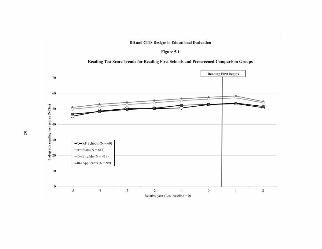
0
10
20
30
40
50
60
70
-5 -4 -3 -2 -1 0 1 2
3rd-
grad
e re
adin
g te
st sc
ores
(NC
Es)
Relative year (Last baseline = 0)
DD and CITS Designs in Educational Evaluation
Figure 5.1
Reading Test Score Trends for Reading First Schools and Prescreened Comparison Groups
RF Schools (N = 69)
State (N = 611)
Eligible (N = 419)
Applicants (N = 99)
Reading First begins
62
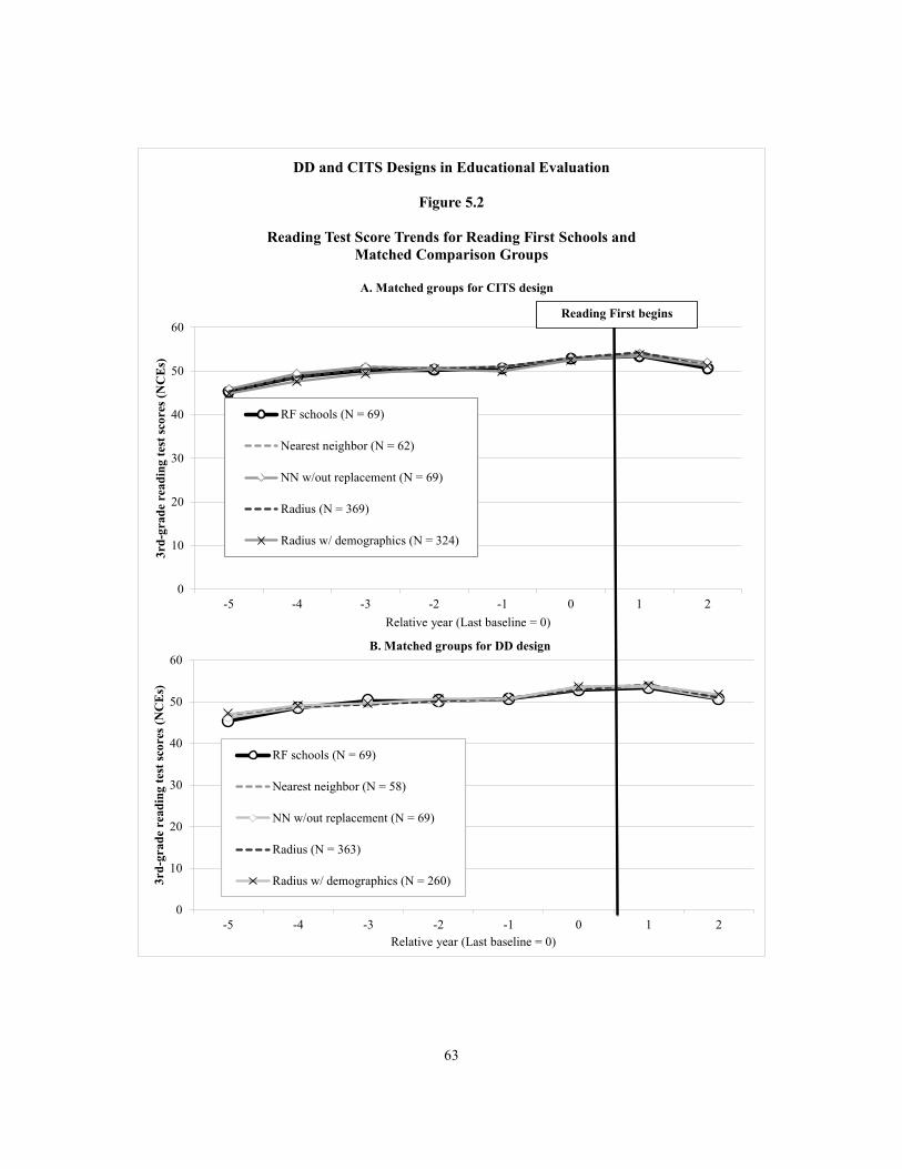
63
0
10
20
30
40
50
60
-5 -4 -3 -2 -1 0 1 2
3rd-
grad
e re
adin
g te
st sc
ores
(NC
Es)
Relative year (Last baseline = 0)
DD and CITS Designs in Educational Evaluation
Figure 5.2
Reading Test Score Trends for Reading First Schools and Matched Comparison Groups
RF schools (N = 69)
Nearest neighbor (N = 62)
NN w/out replacement (N = 69)
Radius (N = 369)
Radius w/ demographics (N = 324)
0
10
20
30
40
50
60
-5 -4 -3 -2 -1 0 1 2
3rd-
grad
e re
adin
g te
st sc
ores
(NC
Es)
Relative year (Last baseline = 0)
B. Matched groups for DD design
RF schools (N = 69)
Nearest neighbor (N = 58)
NN w/out replacement (N = 69)
Radius (N = 363)
Radius w/ demographics (N = 260)
Reading First begins
A. Matched groups for CITS design

64
-0.0260.008 0.003 0.000
-0.035-0.017 -0.023 -0.021
-0.20
-0.15
-0.10
-0.05
0.00
0.05
0.10
0.15
0.20
0.25
RD design (N= 99; SE =0.075; p =
0.725)
State (N =611; SE =0.032; p =
0.81)
Eligible (N =419; SE =0.034; p =
0.923)
Applicants (N= 99; SE =
0.045; p = 1)
Nearestneighbor (N =
62; SE =0.048; p =
0.461)
NN w/outreplacement
(N = 69; SE =0.046; p =
0.711)
Radius (N =369; SE =0.025; p =
0.358)
Radius w/demographics(N = 324; SE= 0.026; p =
0.419)
Effe
ct si
ze
Year 1
0.057 0.049 0.034
-0.032 -0.038 -0.051-0.008
-0.032
-0.35-0.30-0.25-0.20-0.15-0.10-0.050.000.050.100.150.200.25
RD design (N= 99; SE =0.072; p =
0.434)
State (N =611; SE =0.036; p =
0.175)
Eligible (N =419; SE =0.038; p =
0.38)
Applicants (N= 99; SE =0.05; p =
0.525)
Nearestneighbor (N =
62; SE =0.053; p =
0.48)
NN w/outreplacement
(N = 69; SE =0.051; p =
0.322)
Radius (N =369; SE =0.028; p =
0.781)
Radius w/demographics(N = 324; SE= 0.029; p =
0.272)
Effe
ct si
ze
Year 2
DD and CITS Designs in Educational Evaluation
Figure 5.3
Estimated Impact on Reading Scores by Comparison Group, CITS Design(N = number of comparison schools, SE = standard error, p = p-value)

65
-0.026
0.019 0.012 0.012-0.012 -0.009
-0.031
0.004
-0.20
-0.15
-0.10
-0.05
0.00
0.05
0.10
0.15
0.20
0.25
RD design (N= 99; SE =0.075; p =
0.725)
State (N =611; SE =0.029; p =
0.523)
Eligible (N =419; SE =0.031; p =
0.701)
Applicants (N= 99; SE =0.04; p =
0.76)
Nearestneighbor (N =
58; SE =0.046; p =
0.795)
NN w/outreplacement
(N = 69; SE =0.042; p =
0.824)
Radius (N =363; SE =0.023; p =
0.177)
Radius w/demographics(N = 260; SE= 0.027; p =
0.895)
Eff
ect s
ize
Year 1
0.057 0.059 0.040
-0.019 -0.0260.000 -0.012 -0.025
-0.35
-0.30
-0.25
-0.20
-0.15
-0.10
-0.05
0.00
0.05
0.10
0.15
0.20
0.25
RD design (N= 99; SE =0.072; p =
0.434)
State (N =611; SE =0.029; p =
0.043)
Eligible (N =419; SE =0.031; p =
0.197)
Applicants (N= 99; SE =0.04; p =
0.639)
Nearestneighbor (N =
58; SE =0.046; p =
0.575)
NN w/outreplacement
(N = 69; SE =0.042; p =
0.991)
Radius (N =363; SE =0.023; p =
0.588)
Radius w/demographics(N = 260; SE= 0.027; p =
0.352)
Eff
ect s
ize
Year 2
DD and CITS Designs in Educational EvaluationFigure 5.4
Estimated Impact on Reading Scores by Comparison Group, DD Design(N = number of comparison schools, SE = standard error, p = p-value)
66
size (MDES) and the ability to detect impacts if they exist; in Year 1, for example, the MDES is 0.13 for the nearest neighbor method and 0.06-0.07 for the radius method.64
• Matching with replacement (“nearest neighbor”) versus without replacement (“NN w/out replacement”): There does not appear to be any notable benefit to choosing schools without replacement. Matching without replacement does increase the sample size by a small amount, but this does not appreciably reduce the standard error.
• Matching on test scores (“radius”) versus matching on test scores and demographics (“radius w/ demographics”): There is no empirical benefit to matching on demographic characteristics in addition to test scores. Bias estimates for these two approaches are not statistically different from each other, and their standard errors are also similar (ranging from 0.02 to 0.03). This happens because adding demographics to the matching process produces almost the same comparison group as matching on pretests alone.65 These results may be specific to our study, however. Recall that we use at least three years of baseline data for matching in situations where only one or two years of pretest data are available; also matching on demographic characteristics might produce a different (and more credible) comparison group.
• Prescreened groups (“state” and “eligible”) versus matched groups: There is no evidence of bias for the two prescreened (unmatched) groups or for the matched groups. However, the matched groups have two distinct advantages over the prescreened groups. First, impact estimates from the matched groups have greater face validity, because they are more similar to the Reading First schools with respect to baseline test scores (whereas the two prescreened groups are higher achieving than the Reading First schools). Second, impact estimates from some matched groups are also more precise. In Year 1, for example, the standard error for the radius matching method is 73 percent of the size of the standard error for the CITS impact estimate based on “eligible” schools, even though the latter group is larger. This happens because the matching process decreases the variability in test scores among schools in the “radius” comparison group relative to the “eligible” group.
64The MDES is 2.8 times the standard error of the estimated impact (in effect size). 65Among comparison schools in the “radius” comparison group, 69 percent are also included in the
“radius w/ demographics” group. For the math analysis (next section), the overlap between groups is 90 percent. See Tables C.4 and C.5.

67
• “Applicants” versus matched groups: The estimated bias does not statistically differ for matched comparison groups compared with “applicants.” However, as noted earlier, radius matching (which yields a larger comparison group) is superior in terms of precision. In Year 1, for example, the standard error for the CITS impact estimate based on the radius method is about 56 percent of the size of the standard error for the impact based on applicants.
In summary, we conclude that radius matching confers greater precision while still providing impact estimates that are internally valid.
Impacts on Math Scores Our findings about bias — and differences in bias — also hold for math scores, so we discuss them only briefly in this section. The consistency of the results across reading and math lends strength to our conclusions.
Figures 5.5 and 5.6 plot the trend in math test scores (in NCEs) for Reading First schools and the comparison groups. Similar to reading test scores, test score growth for Reading First schools was minimal (flat) in the baseline period. With the exception of the “state” and “eligible” groups — which are higher achieving — baseline test scores for Reading First schools are very similar to those for comparison schools (Figure 5.5).
Figures 5.7 and 5.8 present the estimated impact on math scores for the CITS design and DD designs, while Table 5.2 presents statistical tests of the estimated bias for each impact estimate. The range of bias estimates for math (-0.12 to 0.05) is similar to the range of the estimated bias for reading impacts. None of the bias estimates for math are statistically significant.66
Our conclusions about differences in bias (and precision) across comparison groups are the same for impacts on math scores as for impacts on reading. That is, we conclude that radius matching provides impact estimates that are both internally valid and relatively more precise.
66As seen in Figures 5.7 and 5.8, some of the DD and CITS impact estimates are statistically different
from zero. However, as already discussed, we do not use the statistical significance of individual impact estimates as a criterion to evaluate bias, due to differences in sample size (and therefore precision) across the impact estimates. The more relevant hypothesis test is whether the estimated bias is statistically significant (based on bootstrapped standard errors) presented in Table 5.2.
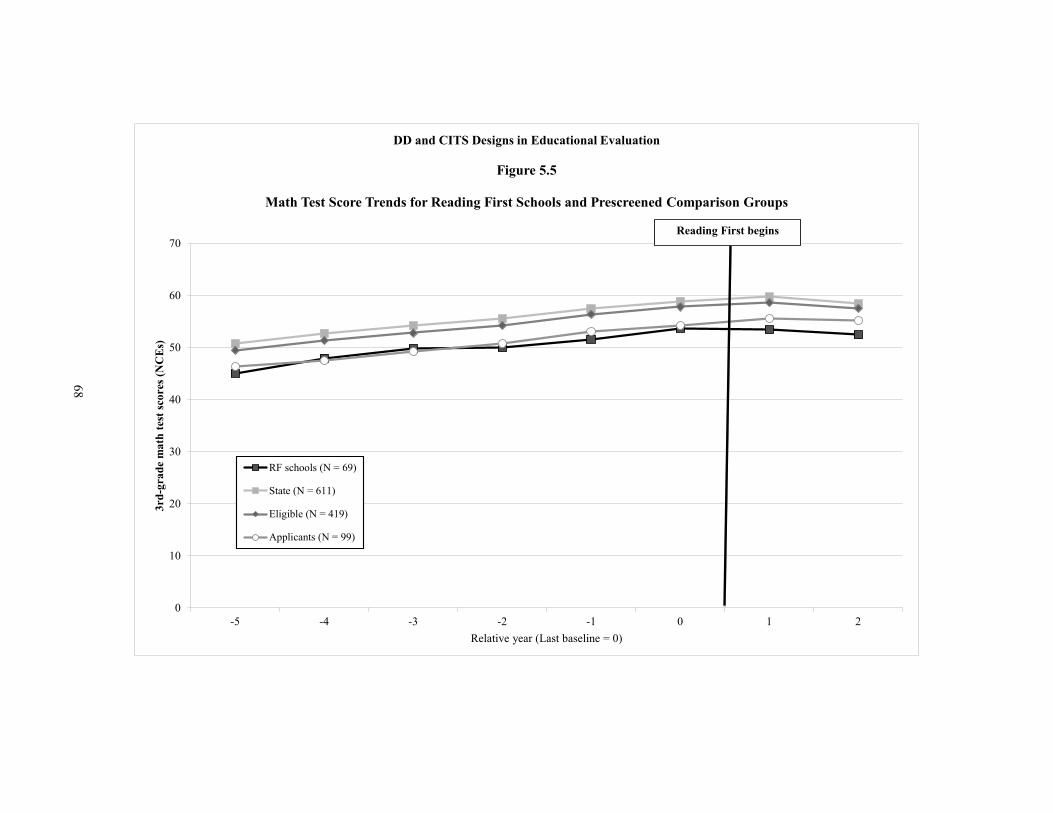
0
10
20
30
40
50
60
70
-5 -4 -3 -2 -1 0 1 2
3rd-
grad
e m
ath
test
scor
es (N
CEs
)
Relative year (Last baseline = 0)
DD and CITS Designs in Educational Evaluation
Figure 5.5
Math Test Score Trends for Reading First Schools and Prescreened Comparison Groups
RF schools (N = 69)
State (N = 611)
Eligible (N = 419)
Applicants (N = 99)
Reading First begins
68
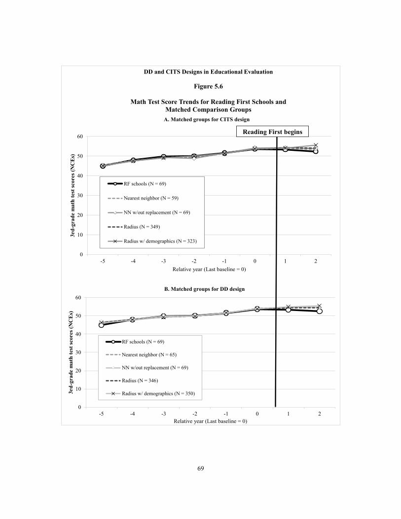
69
0
10
20
30
40
50
60
-5 -4 -3 -2 -1 0 1 2
3rd-
grad
e m
ath
test
scor
es (N
CE
s)
Relative year (Last baseline = 0)
DD and CITS Designs in Educational Evaluation
Figure 5.6
Math Test Score Trends for Reading First Schools and Matched Comparison Groups
RF schools (N = 69)
Nearest neighbor (N = 59)
NN w/out replacement (N = 69)
Radius (N = 349)
Radius w/ demographics (N = 323)
0
10
20
30
40
50
60
-5 -4 -3 -2 -1 0 1 2
3rd-
grad
e m
ath
test
scor
es (N
CE
s)
Relative year (Last baseline = 0)
B. Matched groups for DD design
RF schools (N = 69)
Nearest neighbor (N = 65)
NN w/out replacement (N = 69)
Radius (N = 346)
Radius w/ demographics (N = 350)
Reading First begins
A. Matched groups for CITS design
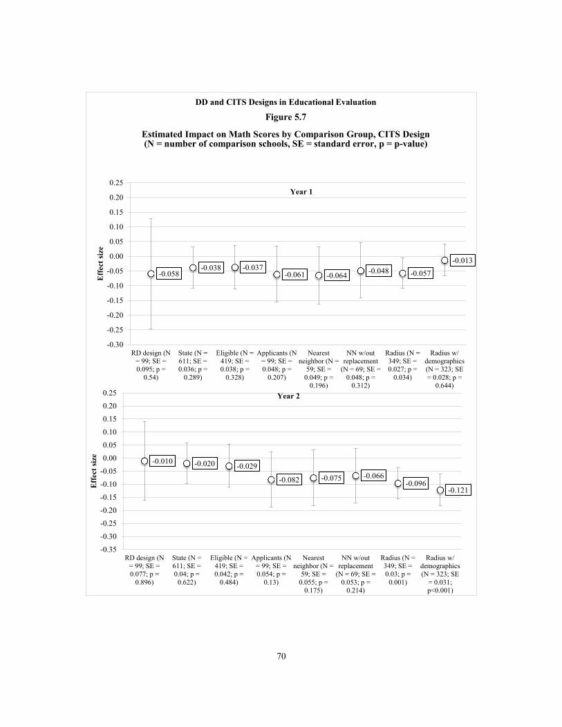
70
-0.058-0.038 -0.037
-0.061 -0.064 -0.048 -0.057
-0.013
-0.30
-0.25
-0.20
-0.15
-0.10
-0.05
0.00
0.05
0.10
0.15
0.20
0.25
RD design (N= 99; SE =0.095; p =
0.54)
State (N =611; SE =0.036; p =
0.289)
Eligible (N =419; SE =0.038; p =
0.328)
Applicants (N= 99; SE =0.048; p =
0.207)
Nearestneighbor (N =
59; SE =0.049; p =
0.196)
NN w/outreplacement
(N = 69; SE =0.048; p =
0.312)
Radius (N =349; SE =0.027; p =
0.034)
Radius w/demographics(N = 323; SE= 0.028; p =
0.644)
Eff
ect s
ize
Year 1
-0.010 -0.020 -0.029
-0.082 -0.075 -0.066-0.096
-0.121
-0.35
-0.30
-0.25
-0.20
-0.15
-0.10
-0.05
0.00
0.05
0.10
0.15
0.20
0.25
RD design (N= 99; SE =0.077; p =
0.896)
State (N =611; SE =0.04; p =
0.622)
Eligible (N =419; SE =0.042; p =
0.484)
Applicants (N= 99; SE =0.054; p =
0.13)
Nearestneighbor (N =
59; SE =0.055; p =
0.175)
NN w/outreplacement
(N = 69; SE =0.053; p =
0.214)
Radius (N =349; SE =0.03; p =
0.001)
Radius w/demographics(N = 323; SE
= 0.031;p<0.001)
Eff
ect s
ize
Year 2
DD and CITS Designs in Educational Evaluation
Figure 5.7
Estimated Impact on Math Scores by Comparison Group, CITS Design(N = number of comparison schools, SE = standard error, p = p-value)

71
-0.058-0.034 -0.037
-0.057 -0.059 -0.058 -0.056 -0.070
-0.30
-0.25
-0.20
-0.15
-0.10
-0.05
0.00
0.05
0.10
0.15
0.20
0.25
RD design (N= 99; SE =0.095; p =
0.54)
State (N =611; SE =0.033; p =
0.304)
Eligible (N =419; SE =0.035; p =
0.293)
Applicants (N= 99; SE =0.044; p =
0.193)
Nearestneighbor (N =
65; SE =0.043; p =
0.168)
NN w/outreplacement
(N = 69; SE =0.043; p =
0.175)
Radius (N =346; SE =0.025; p =
0.028)
Radius w/demographics(N = 350; SE= 0.025; p =
0.005)
Eff
ect s
ize
Year 1
-0.010 -0.019 -0.034-0.082
-0.105 -0.107 -0.101-0.127
-0.35
-0.30
-0.25
-0.20
-0.15
-0.10
-0.05
0.00
0.05
0.10
0.15
0.20
0.25
RD design (N= 99; SE =0.077; p =
0.896)
State (N =611; SE =0.033; p =
0.572)
Eligible (N =419; SE =0.035; p =
0.323)
Applicants (N= 99; SE =0.044; p =
0.06)
Nearestneighbor (N =
65; SE =0.043; p =
0.015)
NN w/outreplacement
(N = 69; SE =0.043; p =
0.013)
Radius (N =346; SE =
0.025;p<0.001)
Radius w/demographics(N = 350; SE
= 0.025;p<0.001)
Eff
ect s
ize
Year 2
DD and CITS Designs in Educational EvaluationFigure 5.8
Estimated Impact on Math Scores by Comparison Group, DD Design(N = number of comparison schools, SE = standard error, p = p-value)
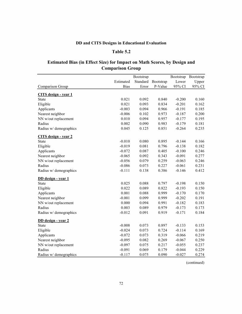
72
Bootstrap Bootstrap BootstrapEstimated Standard Bootstrap Lower Upper
Comparison Group Bias Error P-Value 95% CI 95% CI
CITS design - year 1State 0.021 0.092 0.840 -0.200 0.160Eligible 0.021 0.093 0.834 -0.201 0.162Applicants -0.003 0.094 0.966 -0.191 0.185Nearest neighbor -0.006 0.102 0.973 -0.187 0.200NN w/out replacement 0.010 0.094 0.957 -0.177 0.195Radius 0.002 0.090 0.983 -0.179 0.181Radius w/ demographics 0.045 0.125 0.851 -0.264 0.235
CITS design - year 2State -0.010 0.080 0.895 -0.144 0.166Eligible -0.019 0.081 0.796 -0.138 0.182Applicants -0.072 0.087 0.405 -0.100 0.246Nearest neighbor -0.065 0.092 0.343 -0.091 0.277NN w/out replacement -0.056 0.079 0.259 -0.063 0.246Radius -0.086 0.073 0.227 -0.061 0.231Radius w/ demographics -0.111 0.138 0.386 -0.146 0.412
DD design - year 1State 0.025 0.088 0.797 -0.198 0.150Eligible 0.022 0.089 0.822 -0.193 0.150Applicants 0.001 0.088 0.999 -0.170 0.170Nearest neighbor -0.001 0.099 0.999 -0.202 0.191NN w/out replacement 0.000 0.094 0.991 -0.182 0.183Radius 0.003 0.089 0.979 -0.173 0.173Radius w/ demographics -0.012 0.091 0.919 -0.171 0.184
DD design - year 2State -0.008 0.073 0.897 -0.133 0.153Eligible -0.024 0.073 0.724 -0.114 0.169Applicants -0.072 0.073 0.319 -0.066 0.219Nearest neighbor -0.095 0.082 0.269 -0.067 0.250NN w/out replacement -0.097 0.075 0.217 -0.055 0.237Radius -0.091 0.069 0.179 -0.044 0.229Radius w/ demographics -0.117 0.075 0.090 -0.027 0.274
(continued)
DD and CITS Designs in Educational Evaluation
Table 5.2
Estimated Bias (in Effect Size) for Impact on Math Scores, by Design and Comparison Group
73
NOTES: The estimated bias is equal to the estimated impact based on the relevant comparison group minus the estimated impact from the RD design, using the actual data. The standard error, p-value, and confidence intervals for the bias are obtained using bias estimates from bootstrapped samples (1,000 iterations). The standard error is the standard deviation of bias estimates across iterations. The p-value is obtained by assuming that the distribution for bias is normally distributed. The confidence intervals are the 2.5th and 97.5th percentiles of the bias estimates across iterations. All bias estimates, standard errors, and confidence intervals are shown in effect size based on a standard deviation of 21.06, which is the student-level standard deviation for scores in NCEs.
Table 5.2 (continued)

75
Section 6
Discussion
Having reviewed the results, we can now take stock of our research questions and make recommendations based on the findings.
• Can the comparative interrupted time series (CITS) and difference-in-difference (DD) designs provide internally valid estimates of the impact of a school-level intervention, even when it is not possible to use a geographically local comparison group?
Overall, our findings suggest that the CITS and DD designs can provide internally valid estimates of program impacts, even when it is not possible to restrict the comparison pool to the same set of districts as the treatment group. Statistical tests confirm that the estimated bias is not statistically significant for any of the impact estimates. These results are consistent across comparison groups and matching methods, across implementation years and across subject areas.
This is an important finding, because randomized experiments at the school level are not always politically feasible, and regression discontinuity (RD) designs can have limited power when sample sizes are small (as indicated by the larger confidence intervals for this design in Figures 5.2 and 5.7). For example, the minimum detectable effect size (MDES) for the estimated impact of Reading First on reading scores in Year 1 is 0.21 based on the RD design, compared with 0.13 for the nearest neighbor method and 0.06-0.07 for the radius method. In addition, there are also challenges to using the RD design in practice — many evaluations do not lend themselves to using an RD design.
It is also reassuring that the comparison group does not need to be “local” to obtain internally valid estimates of impacts. As noted earlier, there are situations in which it may not be appropriate (or possible) to restrict the comparison group to schools in the same districts as the treatment schools — for example, when there is spillover to other schools in the district. Where feasible, comparison schools should be from the same set of districts as the treatment schools, but this does not appear to be a necessary condition for validity.
• How do the CITS design and the DD design compare with respect to bias reduction and precision?
Empirically, our study does not provide much scope for demonstrating the advantages of using the CITS design (based on four+ years of pretest scores) instead of the DD design (based on only three or fewer years of pretest scores). We find that the CITS and DD designs

76
both produce internally valid estimates of Reading First impacts and that the estimated bias does not differ across the two designs. Their precision is also very similar.
However, the internal validity of the DD design in this case may be specific to our study and may not generalizable to other contexts. In the first instance, the baseline slope in test scores is similar for Reading First schools and the comparison schools. Had the baseline growth in test scores been different across the two groups, the DD design would have produced biased estimates of impacts. (This is a realistic scenario, because when very few baseline data points are available, one cannot match schools on baseline trends.) Second, the DD design used in this paper is especially strong and perhaps atypical, because it makes use of three years of baseline data. As discussed earlier, having three years of data (as opposed to one or two) strengthens the rigor of the design, because it then becomes possible to match on multiple years of pretest scores and, by extension, to choose a more credible comparison group. Had fewer years of baseline data been used, the DD design might have produced biased results, because baseline slopes might have differed between Reading First schools and the comparison group. This question will be examined in a future paper.
With respect to precision, the two designs produce impact estimates with similar standard errors. This is because our study looks at shorter-term impacts only. As explained earlier, standard errors from the DD design do not account for the additional uncertainty in test score projections in the follow-up period, while the CITS design does (correctly) account for such forecasting error. For this reason, CITS standard errors are larger than DD standard errors, and the standard error of CITS impact estimates increases for projections further out in time. In this study, it is only possible to estimate short-term impacts (first and second follow-up year), and in these years there is little difference between the precision of CITS and DD impact estimates.
• Can the precision of impact estimates from the CITS and DD designs be improved without compromising causal validity, through the choice of matching method (and thus the resulting sample sizes)?
Based on our findings, it is indeed possible to improve the precision of impact estimates without undermining their causal validity. Overall, we conclude that when pretest scores are available for matching, all matching methods produce internally valid impact estimates. This corroborates the findings of prior validation studies. Therefore, one can choose the selection method that will maximize precision.
The most effective means of increasing the precision of DD or CITS impact estimates is to use radius (one-to-many) matching. In the context of Reading First, for example, standard errors from this method are half that of other methods, because it produces a larger comparison

77
group. By extension, the MDES based on radius matching will be half that of the MDES for other methods.
Another strategy for increasing precision (the sample size) is to match without replacement. However, in the case of Reading First, matching without replacement does not improve precision by a noteworthy amount. This is probably because optimal matching (that is, matching without replacement) is most effective for improving precision when the comparison pool for matching is small and when there is intense competition for comparison schools (Gu and Rosenbaum, 1993). When there are few schools from which to choose, and matching is conducted with replacement, a given comparison school will be matched to multiple treatment schools, so in fact there could be few “unique” schools in the comparison group. In this situation, matching without replacement is better, because it will yield a relatively larger comparison group and improve precision. In contrast, when the matching pool is large, competition for comparison schools is less intense, so it is less likely that a comparison school will serve as the “match” for multiple treatment schools when matching with replacement. In this situation, the sample size gains to matching without replacement are minimal (as they are in the case of Reading First). In our study, the pool of “eligible” comparison schools is large (419 schools), which is probably why matching without replacement does not appreciably increase the sample size or improve precision.
Another way of increasing the sample size is to use, as a comparison group, all “untreated” schools in the state or all schools eligible for the intervention. In our study, we find that estimated impacts based on these larger comparison groups are internally valid; previous studies have found a similar result (Fortson, Verbitsky-Savitz, Kopa, and Gleason, 2012). However, these larger “unmatched” groups fail an important requirement — they have much higher test scores at baseline, and therefore they lack “face validity” as a source of counterfactual outcomes for Reading First schools. This is likely to be true in most evaluations — schools that participate in an intervention are typically observably different than other schools in the state or district. Moreover, even though the sample size is smaller for the radius method than when using all schools in the state as a comparison group, estimates from the radius method are actually more precise, because the matching process reduces the heterogeneity in test scores in the sample. Therefore, the radius matching method is preferred — its results have both more face validity and greater precision.
• Is bias reduction stronger or weaker when both pretests and baseline demographic characteristics are used for matching as opposed to pretests only?
We find that matching on pretests and baseline demographic characteristics does not further reduce bias. In other words, matching on pretest scores alone is sufficient to ensure that

78
the comparison group provides the right counterfactual outcomes for Reading First schools in the follow-up period.
However, we caution that this conclusion may be applicable only to school-level evaluations. As noted in the introduction, other studies have found that further matching on demographic characteristics does substantially reduce bias (Steiner, Cook, Shadish, and Clark, 2010). In our study, pretest scores are sufficient — and demographics do not help — because baseline test scores are an especially powerful predictor of future test scores. This happens for two reasons. First, we use multiple years of baseline test scores for matching (three or six) rather than just one, which strengthens the extent to which baseline scores can predict scores in the follow-up period. Second, our analysis is conducted at the school level rather than at the student level. School-level test scores are more reliable (less noisy) that student-level scores, and by extension baseline test scores are more predictive of future test scores at the school level. The fact that both test scores and demographics are more reliably measured at the school level also increases the correlation between these two sets of measures, and therefore reduces the amount of additional information provided by demographics once test scores have been taken into account in the matching process.
Recommendations
Based on these findings, and assuming that pretest data are available for matching, we make the following recommendations:
• Researchers should try to obtain at least four years of pretest data, so that a CITS design can be used to estimate impacts. The main lesson from our analysis is that is important to obtain as many years of pretest data as possible. With four or more years of test scores, one can ensure that treatment and comparison schools have similar baseline test scores and slopes, and use a CITS design to estimate impacts.67 However, if only three or fewer years of available pretest data are available, the slope of the baseline trend cannot be estimated and it is impossible to determine whether the treatment and comparison groups were on similar growth trajectories before the intervention began. By extension, impact estimates from the DD design might not be internally valid, and frustratingly, there would be no way to convincingly determine whether they are or not. In this situation, researchers should be very circumspect about the causal validity and interpretation of their findings.
67Of course, it may be possible to have too many years of pretest data. One should not use pretest scores
that happened in the distant past, since these test scores are likely irrelevant for predicting future outcomes and may bias the prediction.

79
• Radius matching (one-to-many) should be used where feasible. We recommend using the radius matching method to improve precision when the following conditions are met: (a) the candidate pool is large or at least as big as the treatment group, and (b) two or more years of pretest data are available. We do not recommend using this method unless two years of pretest data are available, because this is the minimum amount of data needed to determine the “optimal” radius.68 If only one year of baseline test scores is available, then the optimal radius cannot be determined, and instead the radius must be selected based on ad hoc methods, which could introduce bias into the impact estimates. Our recommendation to use radius matching also assumes that there is no cost constraint on collecting follow-up test scores for more schools and that the “eligible” candidate pool for choosing comparison schools is sufficiently large to allow multiple matches for each treatment school. Using a radius matching approach is also a more rigorous approach than using all schools in the state or all eligible schools as a comparison group, because the radius method will produce a comparison group that looks more similar to the treatment group with respect to pretest scores and demographics, which lends added credibility to the comparison group as a source of counterfactual outcomes.
• If the candidate pool is too small for radius matching, precision can be improved either by using “optimal” nearest neighbor matching or by using “applicants” as a comparison group. In some educational evaluations, the pool of potential comparison schools could be quite small if the geographical scope of the intervention is narrow. For example, if the intervention being evaluated is located in only one school district, the eligible candidate pool will be limited to schools in the district. If the candidate pool is small, radius matching may not be a feasible strategy, because competition for matches is intense and it is less likely that there will be many “good” matches for each treatment school. In this situation, researchers have two options. The first is to use nearest neighbor (one-to-one) matching to choose schools from the pool of candidates; the second option is to use the subgroup of all nonwinning “applicants” as a comparison group, assuming that information on application status is known. The choice between these two strategies depends on the number of nonwinning applicants; if it is larger than the number of treatment schools (successful applicants), using
68Recall that the optimal radius is determined by estimating the “impact” in the last baseline year (which
should be zero). Therefore, this method requires at least two years of baseline data: The last baseline year which serves as the “follow-up” year, plus at least one other baseline year.
80
nonwinning applicants will provide a larger comparison group than using nearest neighbor matching, and therefore better precision. Conversely, if there are fewer nonwinning applicants than schools in the treatment group, the nearest neighbor strategy should be used because it will provide a larger comparison group. In this case, researchers should conduct matching without replacement (optimal matching), since it will produce a relatively larger comparison group than matching with replacement (and therefore more precise estimates). It has also been argued that when there are few “good” matches for the treatment group (as may happen when the pool of comparison candidates is relatively small), optimal matching can produce comparison groups that are more similar to the treatment group and therefore have greater face validity (Gu and Rosenbaum, 1993).
• Matching on demographic characteristics should be conducted as a sensitivity test. Based on our findings, matching on demographic characteristics (in addition to pretest scores) does not add anything to the validity or precision of the impact estimates from a DD or CITS design. In theory, however, there are reasons both for and against matching on demographic characteristics. On the one hand, adding demographics to the matching process could increase the credibility of the matching process and the resulting comparison group. On the other hand, if the pool of candidate schools is small, it may be difficult to find schools that look similar to the treatment group on both pretests and demographic characteristics. In this situation, adding demographics to the mix could impose a constraint on one’s ability to match schools with respect to baseline test scores. Matching on pretest scores should be prioritized because they are the strongest predictor of future test scores. Therefore, we recommend matching on pretest scores in the primary analysis, and then matching on pretests and demographics as a sensitivity test.
It is important to note that our findings and recommendations may be limited to studies whose conditions are similar to those of the Reading First evaluation, and in particular to school-level evaluations. Therefore, in practice, we recommend that researchers conduct their own “validation” exercise to choose the right comparison group method. In a “real world” evaluation the “true” impact of the program is not known. However, the right selection method can be chosen based on a different benchmark — the impact of the program in the last baseline year, which should be zero. The validation exercise would proceed as follows: (1) identify “matched” comparison schools using all baseline years except the last one, and (2) estimate “impacts” in the last baseline year using the resulting comparison groups(s). The right selection method would be the one that most reliably estimates an impact of zero (that is, the method
81
where the standard error is the smallest but where zero, which by construction is the correct answer, is still included in the confidence interval for the impact estimate).69 Having chosen a “primary” matching method, one would then conduct the matching exercise again, using the chosen method and all years of baseline data. After comparison schools have been selected, one would estimate the impact of the intervention, using a CITS design if there are at least four years of baseline data (and a DD design if there are not). Results based on other matching methods can also be presented, as a sensitivity test.
In conclusion, our findings corroborate those of previous validation studies, showing that nonexperimental designs (in this case the DD and CITS design) can produce internally valid estimates of program impacts when pretest scores are available, regardless of the matching method that is used to select comparison schools. Notably, this is the first study to demonstrate that the CITS design can produce internally valid results. However, our paper also contributes to the literature by showing that (1) using a comparison group that is “local” (that is, from the same set of districts as the treatment schools) is not a necessary condition for obtaining causally valid estimates of program impacts; (2) further matching on demographic characteristics is not necessary in the context of the DD or CITS design; and (3) the precision of impact estimates (and the MDES) can be increased without compromising validity, by matching using the radius method rather than nearest neighbor matching.
69More formally, one could calculate the MSE for each method, based on the estimated impact in the last
baseline year (𝜑𝐿𝐵� ) and its standard error, and then choose the method with the smallest MSE: 𝑀𝑆𝐸�𝐿𝐵 = 𝜑𝐿𝐵�
2 + 𝑣𝑎𝑟(𝜑𝐿𝐵� ).

Appendix A
Specification Tests for the Regression Discontinuity Design

85
This appendix presents the results of the regression discontinuity (RD) specification tests discussed in Section 3:
• “Impact” on characteristics and outcomes that should not be affected by
Reading First: Table A.1 presents the impact of Reading First on school characteristics in the last baseline year. The estimated impact of Reading First on these variables should be zero or not statistically significant. The re-sults shown in this table confirm that Reading First did not have an impact on these characteristics.
• Functional form tests: Table A.2 presents estimated impacts (in effect size) on reading and math scores, based on different functional forms for the rela-tionship between the rating variable and test scores. The type of relationship is indicated in the first column of these tables. The results indicate that re-gardless of which type of model is used, estimated impacts on test scores are not statistically significant.
• Test of difference in slopes: Table A.3 presents tests of the relationship be-tween ratings and test scores (slope) on each side of the cut-off. The results indicate that the slopes are not statistically different, and that we can use an RD model that constrains the slope to be the same on either side of the cut-off. These results also suggest that the estimated impact of Reading First does not differ across schools and that the impact estimates are generalizable to the entire sample (and not just to schools around the cut-off).
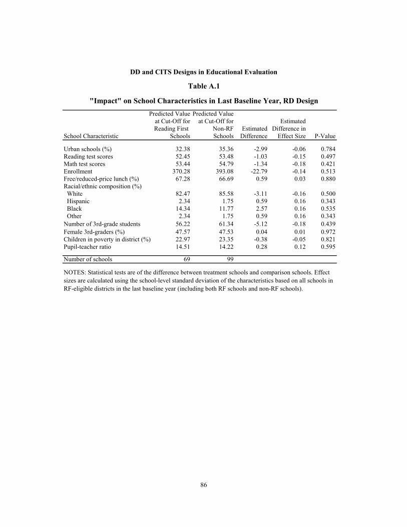
86
Predicted Value Predicted Valueat Cut-Off for at Cut-Off for EstimatedReading First Non-RF Estimated Difference in
School Characteristic Schools Schools Difference Effect Size P-Value
Urban schools (%) 32.38 35.36 -2.99 -0.06 0.784Reading test scores 52.45 53.48 -1.03 -0.15 0.497Math test scores 53.44 54.79 -1.34 -0.18 0.421Enrollment 370.28 393.08 -22.79 -0.14 0.513Free/reduced-price lunch (%) 67.28 66.69 0.59 0.03 0.880Racial/ethnic composition (%) White 82.47 85.58 -3.11 -0.16 0.500 Hispanic 2.34 1.75 0.59 0.16 0.343 Black 14.34 11.77 2.57 0.16 0.535 Other 2.34 1.75 0.59 0.16 0.343Number of 3rd-grade students 56.22 61.34 -5.12 -0.18 0.439Female 3rd-graders (%) 47.57 47.53 0.04 0.01 0.972Children in poverty in district (%) 22.97 23.35 -0.38 -0.05 0.821Pupil-teacher ratio 14.51 14.22 0.28 0.12 0.595
Number of schools 69 99
DD and CITS Designs in Educational Evaluation
Table A.1
"Impact" on School Characteristics in Last Baseline Year, RD Design
NOTES: Statistical tests are of the difference between treatment schools and comparison schools. Effect sizes are calculated using the school-level standard deviation of the characteristics based on all schools in RF-eligible districts in the last baseline year (including both RF schools and non-RF schools).
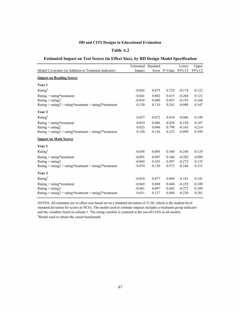
87
Estimated Standard Lower UpperModel Covariates (in Addition to Treatment Indicator) Impact Error P-Value 95% CI 95% CI
Impact on Reading Scores
Year 1Ratinga -0.026 0.075 0.725 -0.174 0.122Rating + rating*treatment -0.041 0.082 0.615 -0.204 0.121Rating + rating2 -0.016 0.089 0.855 -0.193 0.160Rating + rating2 + rating*treatment + rating2*treatment 0.130 0.110 0.241 -0.088 0.347
Year 2Ratinga 0.057 0.072 0.434 -0.086 0.199Rating + rating*treatment 0.019 0.086 0.828 -0.150 0.187Rating + rating2 0.025 0.096 0.798 -0.165 0.214Rating + rating2 + rating*treatment + rating2*treatment 0.150 0.126 0.235 -0.099 0.399
Impact on Math Scores
Year 1Ratinga -0.058 0.095 0.540 -0.246 0.129Rating + rating*treatment -0.091 0.097 0.346 -0.282 0.099Rating + rating2 -0.069 0.103 0.507 -0.272 0.135Rating + rating2 + rating*treatment + rating2*treatment 0.074 0.130 0.573 -0.184 0.331
Year 2Ratinga -0.010 0.077 0.896 -0.161 0.141Rating + rating*treatment -0.065 0.088 0.460 -0.239 0.109Rating + rating2 -0.081 0.097 0.402 -0.272 0.109Rating + rating2 + rating*treatment + rating2*treatment 0.031 0.127 0.808 -0.220 0.281
NOTES: All estimates are in effect size based on on a standard deviation of 21.06, which is the student-level standard deviation for scores in NCEs. The model used to estimate impacts includes a treatment group indicator and the variables listed in column 1. The rating variable is centered at the cut-off (145) in all models. aModel used to obtain the causal benchmark.
DD and CITS Designs in Educational Evaluation
Table A.2
Estimated Impact on Test Scores (in Effect Size), by RD Design Model Specification

88
Estimated EstimatedSlope Slope Estimated Standard
Subject -Year RF Schools Non-RF Schools Difference Error P-Value
Reading scoresYear 1 0.043 0.000 0.042 0.086 0.625Year 2 0.045 -0.062 0.107 0.090 0.237
Math scoresYear 1 0.062 -0.032 0.093 0.097 0.337Year 2 0.082 -0.074 0.156 0.093 0.094
Number of schools 69 99
NOTES: Slopes are scaled in normal curve equivalents (NCEs). Rounding may cause slight discrepancies in calculating differences. The statistical model used to estimate slopes includes the treatment indicator, the rating variable centered on the cut-off of 145, and the interaction between the treatment indicator and the centered rating. The coefficient on the interaction term (in the "Estimated Difference" column) is the difference between the slopes of the RF and non-RF group.
DD and CITS Designs in Educational Evaluation
Table A.3
Relationship Between Test Scores (in NCEs) and Ratings, for Reading First and Non-Reading First Schools

Appendix B
Minimum Detectable Effect Size for Nonexperimental Designs


91
A common way to convey a study’s statistical power is through the minimum detectable effect (MDE) or the minimum detectable effect size (MDES). Formally the MDE is the smallest true program impact that can be detected with a reasonable degree of power (in this case, 80 percent) for a given level of statistical significance (in this case, 5 percent for a two-tailed test). The MDES is the MDE scaled as an effect size — in other words, it is the MDE divided by the standard deviation of the outcome of interest. (In this paper, we use a standard deviation of 21.06, which is the student-level standard deviation for scores in normal curve equivalents.)
For samples with more than about 20 degrees of freedom, the MDES is approximately equal to 2.8 times the standard error of the relevant impact estimate. Once the analysis has been conducted, this calculation is simple because the standard error is known. For example, the MDES presented in this paper are based on the standard errors of the relevant impact estimates.
In the study design phase, however, the standard error is not yet known and must be ap-proximated based on assumptions about the properties of the data and the design that will be used to estimate effects. The formulas for the MDES in the study design phase are described below for each nonexperimental design.
Regression Discontinuity (RD) Design For the RD design, the MDES is calculated as follows (Bloom, 2012):
𝑀𝐷𝐸𝑆 (𝑅𝐷) ≈ 2.8�1
𝑁𝑃(1−𝑃)(1−𝑅𝑇2)
where all variables are defined as before and:
𝑵 = Number of schools (treatment and comparison) 𝑷 = The proportion of schools that are in the treatment group 𝑹𝑻𝟐 = The proportion of variation in treatment status (T) predicted by
the centered rating and other covariates included in the regression discontinuity model
The collinearity between the rating variable and the outcome (𝑅𝑇2) reduces the precision
of impact estimates (or conversely it increases the MDES). Therefore, impact estimates from an RD design generally have more limited power than other potential designs (including the difference-in-difference [DD] and comparative interrupted time series [CITS] designs). See Bloom (2012) for a discussion.

92
DD and CITS Designs In its simplest form, the MDES for a CITS design is calculated as follows:1
𝑀𝐷𝐸𝑆(𝐶𝐼𝑇𝑆) ≈ 2.8 ∗ �1𝑛�
1𝑚𝑡
+ 1𝑚𝑐�1 + 1
𝑇+ �𝑡𝑓−�̅��
2
∑ (𝑡𝑘−�̅�)2𝑘
where:
𝒎𝒕 = Number of treatment schools 𝒎𝒄 = Number of comparison schools n = Number of students per school per academic year. 𝑻 = Number of years of data in the baseline period 𝒕𝒇 = The follow-up year of the impact (= 0 for first follow-up year,
1 for the second, 2 for the third, etc.) �̅� = The average value of the baseline years (where baseline years
are scaled from -1 to –T, where T is the total number of baseline years)
A key feature of CITS estimation is reflected in the last term of the equation:
�𝑡𝑓−𝑡�̅2
∑ (𝑡𝑘 − 𝑡̅)2𝑘
This term accounts for the fact that projections about counterfactual outcomes in the follow-up period (and therefore impacts) are less reliable for time periods that are further away in time. For this reason, the MDES for a CITS design increases as tf increases.
In contrast, the MDES for a DD design is the following:
𝑀𝐷𝐸𝑆(𝐷𝐷) ≈ 2.8 ∗ �1𝑛�
1𝑚𝑡
+ 1𝑚𝑐�1 + 1
𝑇
As seen here, the MDES for the DD design does not include a term to account for de-creases in precision for longer-term impacts, because the DD design assumes that the reliability
1The formulas in this appendix are based on Bloom (1999), but they also include an additional component
for the between-school intraclass correlation to account for the use of school random effects (which are used in our analysis).

93
of counterfactual projections is the same across follow-up periods. In education research, this assumption is likely to be incorrect, in which case the observed precision of the DD design overestimates its true precision.
For this reason, the CITS design provides a better reflection of the true precision of im-pact estimates than a DD design, especially for longer-term impacts.


Appendix C
Characteristics of Comparison Groups


97
This appendix presents supplemental results on the characteristics of schools in the difference-in-difference (DD) and comparative interruptive time series (CITS) analyses:
• Tables C.1 to C.3 present the characteristics of schools used to estimate im-pacts on math scores.
• Tables C.4 and C.5 show the amount of overlap between schools in the matched comparison groups used to estimate impacts, for reading and math, respectively.

98
RFSchool Characteristic Schools State Eligible Applicants
Baseline math test scores
Predicted score in last baseline year 53.54 58.97 57.84 54.29(0.72) X (0.57) X (0.1)
Baseline trend (6 years) 1.54 1.61 1.66 1.64(0.05) (0.08) (0.07)
Demographic characteristics (last baseline year)
Urban schools (%) 37.68 34.26 35.80 22.22(-0.07) (-0.04) (-0.32) X
Enrollment 382.61 409.56 400.13 362.55(0.17) (0.11) (-0.13)
Free/reduced-price lunch (%) 65.64 53.96 57.97 70.73(-0.56) X (-0.37) X (0.24)
Racial/ethnic composition (%) White 81.35 88.31 85.73 88.36
(0.37) X (0.23) (0.37) X Hispanic 2.50 1.60 1.68 1.35
(-0.24) (-0.22) (-0.31) X Black 15.17 9.16 11.54 9.70
(-0.37) X (-0.22) (-0.33) X Other 2.50 1.60 1.68 1.35
(-0.24) (-0.22) (-0.31) XNumber of 3rd-grade students 59.97 62.89 60.59 52.04
(0.1) (0.02) (-0.28) XFemale 3rd-graders (%) 47.91 47.48 47.56 46.69
(-0.09) (-0.08) (-0.26) XChildren in poverty in district (%) 22.00 20.66 22.45 25.75
(-0.19) (0.06) (0.54) XPupil-teacher ratio 14.47 15.57 15.40 14.32
(0.45) X (0.38) X (-0.06)
Number of schools 69 611 419 99
NOTES: Values shown in parentheses are the difference between RF and comparison schools in effect size. Effect sizes are calculated using the school-level standard deviation based on all schools in RF-eligible districts in the last baseline year (including both RF schools and non-RF schools). Differences greater than 0.25 SD are indicated with an "X." Statistical tests of the difference between Reading First schools and comparison schools are not shown, because the precision of the estimated difference varies across the comparison groups. (For a given effect size, larger comparison groups are more likely to be deemed statistically different from RF schools.)
Comparison Groups
Table C.1
Characteristics of Reading First Schools and Prescreened Comparison Groups (for Impacts on Math Scores)
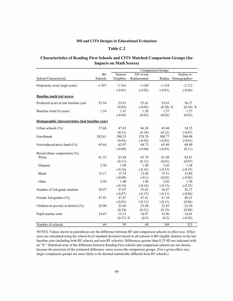
99
RF Nearest NN w/out Radius w/School Characteristic Schools Neighbor Replacement Radius Demographics
Propensity score (logit scale) -1.507 -1.516 -1.520 -1.518 -1.712(-0.01) (-0.02) (-0.01) (-0.06)
Baseline math test scores
Predicted score in last baseline year 53.54 53.91 53.41 55.63 56.27(0.05) (-0.02) (0.28) X (0.36) X
Baseline trend (6 years) 1.54 1.47 1.58 1.57 1.57(-0.05) (0.03) (0.02) (0.02)
Demographic characteristics (last baseline year)
Urban schools (%) 37.68 47.83 46.38 43.48 34.33(0.21) (0.18) (0.12) (-0.07)
Enrollment 382.61 390.25 378.70 380.77 380.98(0.05) (-0.02) (-0.01) (-0.01)
Free/reduced-price lunch (%) 65.64 63.97 64.73 65.49 68.00(-0.08) (-0.04) (-0.01) (0.11)
Racial/ethnic composition (%) White 81.35 83.49 83.70 81.48 82.67
(0.11) (0.12) (0.01) (0.07) Hispanic 2.50 1.90 1.90 2.02 1.58
(-0.16) (-0.16) (-0.13) (-0.25) Black 15.17 13.74 13.48 15.51 14.89
(-0.09) (-0.1) (0.02) (-0.02) Other 2.50 1.90 1.90 2.02 1.58
(-0.16) (-0.16) (-0.13) (-0.25)Number of 3rd-grade students 59.97 57.97 55.81 56.87 58.37
(-0.07) (-0.15) (-0.11) (-0.06)Female 3rd-graders (%) 47.91 47.87 47.41 47.38 48.21
(-0.01) (-0.11) (-0.11) (0.06)Children in poverty in district (%) 22.00 23.66 23.49 22.85 22.56
(0.24) (0.21) (0.12) (0.08)Pupil-teacher ratio 14.47 15.13 14.97 14.96 14.41
(0.27) X (0.2) (0.2) (-0.03)
Number of schools 69 59 69 349 323
NOTES: Values shown in parentheses are the difference between RF and comparison schools in effect size. Effect sizes are calculated using the school-level standard deviation based on all schools in RF-eligible districts in the last baseline year (including both RF schools and non-RF schools). Differences greater than 0.25 SD are indicated with an "X." Statistical tests of the difference between Reading First schools and comparison schools are not shown, because the precision of the estimated difference varies across the comparison groups. (For a given effect size, larger comparison groups are more likely to be deemed statistically different from RF schools.)
Comparison Groups
Characteristics of Reading First Schools and CITS Matched Comparison Groups (for Impacts on Math Scores)
Table C.2
DD and CITS Designs in Educational Evaluation
100
RF Nearest NN w/out Radius w/School Characteristic Schools Neighbor Replacement Radius Demographics
Propensity score (logit scale) -1.558 -1.561 -1.561 -1.565 -1.654(-0.004) (-0.004) (-0.01) (-0.04)
Baseline math test scores
Predicted score in last baseline year 53.54 53.46 53.34 55.03 55.46(-0.01) (-0.03) (0.2) (0.25) X
Baseline trend (6 years) 1.54 1.40 1.32 1.42 1.38(-0.11) (-0.16) (-0.09) (-0.12)
Demographic characteristics (last baseline year)
Urban schools (%) 37.68 52.17 52.17 42.09 35.33(0.3) X (0.3) X (0.09) (-0.05)
Enrollment 382.61 423.77 419.96 390.62 377.65(0.26) X (0.23) (0.05) (-0.03)
Free/reduced-price lunch (%) 65.64 60.95 60.53 64.25 65.52(-0.23) (-0.25) (-0.07) (-0.01)
Racial/ethnic composition (%) White 81.35 83.75 82.36 82.17 82.66
(0.13) (0.05) (0.04) (0.07) Hispanic 2.50 2.06 2.23 1.95 2.13
(-0.12) (-0.07) (-0.15) (-0.1) Black 15.17 13.28 14.45 14.94 14.31
(-0.12) (-0.04) (-0.01) (-0.05) Other 2.50 2.06 2.23 1.95 2.13
(-0.12) (-0.07) (-0.15) (-0.1)Number of 3rd-grade students 59.97 66.62 65.43 58.13 58.17
(0.23) (0.19) (-0.06) (-0.06)Female 3rd-graders (%) 47.91 46.83 46.94 47.02 48.28
(-0.23) (-0.21) (-0.19) (0.08)Children in poverty in district (%) 22.00 21.29 21.26 22.90 22.14
(-0.1) (-0.11) (0.13) (0.02)Pupil-teacher ratio 14.47 15.31 15.29 15.12 14.50
(0.34) X (0.33) X (0.26) X (0.01)
Number of schools 69 65 69 346 350
NOTES: Values shown in parentheses are the difference between RF and comparison schools in effect size. Effect sizes are calculated using the school-level standard deviation based on all schools in RF-eligible districts in the last baseline year (including both RF schools and non-RF schools). Differences greater than 0.25 SD are indicated with an "X." Statistical tests of the difference between Reading First schools and comparison schools are not shown, because the precision of the estimated difference varies across the comparison groups. (For a given effect size, larger comparison groups are more likely to be deemed statistically different from RF schools.)
Comparison Groups
DD and CITS Designs in Educational Evaluation
Table C.3
Characteristics of Reading First Schools and DD Matched Comparison Groups (for Impacts on Math Scores)
CITS CITS CITS DD DD DDAppli- Nearest NN w/out CITS Radius w/ Nearest NN w/out DD Radius
Among schools in the following State Eligible cants Neighbor Repl. Radius Demo. Neighbor repl. Radius w/ Demo.comparison groups… (N) (611) (419) (99) (62) (69) (369) (324) (58) (69) (363) (260)
State (611) 100% 69% 16% 10% 11% 60% 53% 9% 11% 59% 43%Eligible (419) 100% 100% 24% 15% 16% 88% 77% 14% 16% 87% 62%Applicants (99) 100% 100% 100% 17% 20% 91% 85% 21% 24% 94% 71%CITS - Nearest neighbor (62) 100% 100% 27% 100% 94% 100% 84% 19% 23% 97% 71%CITS - NN w/out replacement (69) 100% 100% 29% 84% 100% 97% 84% 22% 23% 94% 74%CITS - Radius (369) 100% 100% 24% 17% 18% 100% 82% 15% 18% 94% 68%CITS - Radius, w/ demographics (324) 100% 100% 26% 16% 18% 94% 100% 15% 18% 91% 72%DD - Nearest neighbor (58) 100% 100% 36% 21% 26% 93% 81% 100% 91% 100% 76%DD - NN w/out replacement (69) 100% 100% 35% 20% 23% 94% 83% 77% 100% 100% 75%DD - Radius (363) 100% 100% 26% 17% 18% 95% 81% 16% 19% 100% 69%DD - Radius, w/ demographics (260) 100% 100% 27% 17% 20% 97% 90% 17% 20% 96% 100%
… Percentage that are also in …
NOTES: Value in (Row X, Column Y) = Percentage of schools in the comparison group in Row X that are also part of the comparison group in Column Y. (N) = Sample size of comparison group
DD and CITS Designs in Educational Evaluation
Table C.4
Overlap Between Comparison Groups (for Impacts on Reading)
101
CITS CITS CITS DD DD DDAppli- Nearest NN w/out CITS Radius w/ Nearest NN w/out DD Radius w/
Among schools in the following State Eligible cants Neighbor Repl. Radius Demo. Neighbor Repl. Radius Demo.comparison groups… (N) (611) (419) (99) (59) (69) (349) (323) (65) (69) (346) (350)
State (611) 100% 69% 16% 10% 11% 57% 53% 11% 11% 57% 57%Eligible (419) 100% 100% 24% 14% 16% 83% 77% 16% 16% 83% 84%Applicants (99) 100% 100% 100% 19% 22% 92% 83% 16% 17% 92% 94%CITS - Nearest neighbor (59) 100% 100% 32% 100% 93% 100% 85% 24% 27% 98% 93%CITS - NN w/out replacement (69) 100% 100% 32% 80% 100% 99% 83% 25% 28% 99% 93%CITS - Radius (349) 100% 100% 26% 17% 19% 100% 82% 18% 19% 95% 91%CITS - Radius, w/ demographics (323) 100% 100% 25% 15% 18% 89% 100% 17% 18% 87% 93%DD - Nearest neighbor (65) 100% 100% 25% 22% 26% 98% 85% 100% 92% 100% 94%DD - NN w/out replacement (69) 100% 100% 25% 23% 28% 99% 83% 87% 100% 100% 96%DD - Radius (346) 100% 100% 26% 17% 20% 96% 82% 19% 20% 100% 91%DD - Radius, w/ demographics (350) 100% 100% 27% 16% 18% 91% 86% 17% 19% 90% 100%
NOTES: Value in (Row X, Column Y) = Percentage of schools in the comparison group in Row X that are also part of the comparison group in Column Y.(N) = Sample size of comparison group
… Percentage that are also in …
Overlap Between Comparison Groups (for Impacts on Math)
Table C.5
DD and CITS Designs in Educational Evaluation
102

Appendix D
CITS and DD Impact Estimates


105
This appendix presents coefficient estimates from comparative interruptive time series (CITS) and difference-in-difference (DD) impact models used to estimate impacts on test scores, for each relevant comparison group. In these tables, estimates are shown in their original metric, rather than effect sizes. Tables D.1 and D.2 present estimates from the models used to estimate impacts on reading scores, while Tables D.3 and D.4 present estimates from the analysis of math scores.
106
EstimatedRF Comparison Difference Standard
Comparison Group Schools Schools or Impact Error P-Value
Baseline trendState 1.244 1.256 -0.012 0.142 0.931Eligible 1.244 1.285 -0.041 0.151 0.787Applicants 1.244 1.234 0.010 0.195 0.961Nearest neighbor 1.244 1.137 0.106 0.210 0.613Nearest neighbor w/out replacement 1.244 1.161 0.082 0.205 0.688Radius 1.244 1.207 0.037 0.127 0.773Radius w/ demographics 1.244 1.226 0.018 0.137 0.897
Predicted score in last baseline yearState 52.745 57.692 -4.947 0.771 0.000Eligible 52.745 56.513 -3.767 0.792 0.000Applicants 52.745 53.070 -0.324 0.843 0.701Nearest neighbor 52.745 53.500 -0.754 0.981 0.443Nearest neighbor w/out replacement 52.745 53.048 -0.303 0.975 0.756Radius 52.745 55.075 -2.329 0.682 0.001Radius w/ demographics 52.745 55.001 -2.256 0.714 0.002
Deviation from baseline trend - year 1State -0.580 -0.744 0.164 0.681 0.810Eligible -0.580 -0.650 0.069 0.721 0.923Applicants -0.580 -0.581 0.000 0.938 1.000Nearest neighbor -0.580 0.162 -0.742 1.006 0.461Nearest neighbor w/out replacement -0.580 -0.220 -0.360 0.972 0.711Radius -0.580 -0.099 -0.482 0.524 0.358Radius w/ demographics -0.580 -0.142 -0.439 0.542 0.419
Deviation from baseline trend - year 2State -4.549 -5.579 1.030 0.760 0.175Eligible -4.549 -5.255 0.706 0.804 0.380Applicants -4.549 -3.884 -0.665 1.046 0.525Nearest neighbor -4.549 -3.756 -0.793 1.122 0.480Nearest neighbor w/out replacement -4.549 -3.476 -1.073 1.084 0.322Radius -4.549 -4.386 -0.163 0.585 0.781Radius w/ demographics -4.549 -3.884 -0.665 0.605 0.272
NOTE: Impacts and standard errors are expressed in normal curve equivalents (NCEs).
Model Estimates for Impact on Reading Scores by Comparison Group, CITS Design
Table D.1
DD and CITS Designs in Educational Evaluation

107
EstimatedRF Comparison Difference or Standard
Comparison Group Schools Schools Impact Error P-Value
Baseline meanState 56.413 51.222 5.190 0.750 0.000Eligible 55.213 51.222 3.991 0.769 0.000Applicants 51.796 51.222 0.573 0.813 0.482Nearest neighbor 51.819 51.222 0.596 0.979 0.544Nearest neighbor w/out replacement 51.321 51.222 0.099 0.942 0.916Radius 53.115 51.222 1.893 0.619 0.002Radius w/ demographics 53.078 51.222 1.856 0.660 0.005
Deviation from baseline mean - year 1State 2.186 1.792 0.395 0.617 0.523Eligible 2.186 1.934 0.252 0.658 0.701Applicants 2.186 1.928 0.259 0.845 0.760Nearest neighbor 2.186 2.436 -0.250 0.958 0.795Nearest neighbor w/out replacement 2.186 2.383 -0.197 0.885 0.824Radius 2.186 2.839 -0.652 0.483 0.177Radius w/ demographics 2.186 2.112 0.074 0.564 0.895
Deviation from baseline mean - year 2State -0.538 -1.787 1.249 0.617 0.043Eligible -0.538 -1.386 0.848 0.658 0.197Applicants -0.538 -0.141 -0.397 0.845 0.639Nearest neighbor -0.538 0.000 -0.538 0.958 0.575Nearest neighbor w/out replacement -0.538 -0.529 -0.010 0.885 0.991Radius -0.538 -0.276 -0.262 0.483 0.588Radius w/ demographics -0.538 -0.013 -0.525 0.564 0.352
Model Estimates for Impact on Reading Scores by Comparison Group, DD Design
NOTE: Impacts and standard errors are expressed in normal curve equivalents (NCEs).
DD and CITS Designs in Educational Evaluation
Table D.2

108
EstimatedRF Comparison Difference Standard
Comparison Group Schools Schools or Impact Error P-Value
Baseline trendState 1.544 1.608 -0.063 0.161 0.693Eligible 1.544 1.656 -0.112 0.171 0.513Applicants 1.544 1.643 -0.099 0.212 0.641Nearest neighbor 1.544 1.472 0.072 0.237 0.762NN w/out replacement 1.544 1.582 -0.038 0.225 0.865Radius 1.544 1.571 -0.027 0.144 0.850Radius w/ demographics 1.544 1.571 -0.027 0.152 0.860
Predicted score in last baseline yearState 53.541 58.970 -5.430 0.841 0.000Eligible 53.541 57.835 -4.294 0.865 0.000Applicants 53.541 54.289 -0.748 0.917 0.416Nearest neighbor 53.541 53.915 -0.374 1.049 0.722NN w/out replacement 53.541 53.411 0.129 1.018 0.899Radius 53.541 55.629 -2.089 0.718 0.004Radius w/ demographics 53.541 56.267 -2.727 0.756 0.000
Deviation from baseline trend - year 1State -1.654 -0.859 -0.795 0.749 0.289Eligible -1.654 -0.878 -0.776 0.793 0.328Applicants -1.654 -0.370 -1.284 1.018 0.207Nearest neighbor -1.654 -0.306 -1.348 1.042 0.196NN w/out replacement -1.654 -0.636 -1.019 1.007 0.312Radius -1.654 -0.461 -1.194 0.564 0.034Radius w/ demographics -1.654 -1.384 -0.271 0.585 0.644
Deviation from baseline trend - year 2State -4.178 -3.766 -0.412 0.836 0.622Eligible -4.178 -3.559 -0.619 0.885 0.484Applicants -4.178 -2.457 -1.721 1.136 0.130Nearest neighbor -4.178 -2.598 -1.580 1.162 0.175NN w/out replacement -4.178 -2.782 -1.396 1.124 0.214Radius -4.178 -2.160 -2.018 0.630 0.001Radius w/ demographics -4.178 -1.620 -2.558 0.653 0.000
NOTE: Impacts and standard errors are expressed in normal curve equivalents (NCEs).
Model Estimates for Impact on Math Scores by Comparison Group, CITS Design
Table D.3
DD and CITS Designs in Educational Evaluation

109
EstimatedRF Comparison Difference Standard
Comparison Group Schools Schools or Impact Error P-Value
Baseline meanState 51.744 57.322 -5.578 0.821 0.000Eligible 51.744 56.157 -4.413 0.843 0.000Applicants 51.744 52.674 -0.930 0.886 0.296Nearest neighbor 51.744 51.924 -0.180 0.973 0.854NN w/out replacement 51.744 51.836 -0.092 0.948 0.923Radius 51.744 53.336 -1.592 0.658 0.016Radius w/ demographics 51.744 53.736 -1.992 0.690 0.004
Deviation from baseline mean - year 1State 1.686 2.396 -0.710 0.691 0.304Eligible 1.686 2.456 -0.770 0.732 0.293Applicants 1.686 2.888 -1.201 0.922 0.193Nearest neighbor 1.686 2.937 -1.251 0.906 0.168NN w/out replacement 1.686 2.906 -1.220 0.898 0.175Radius 1.686 2.855 -1.169 0.530 0.028Radius w/ demographics 1.686 3.167 -1.481 0.532 0.005
Deviation from baseline mean - year 2State 0.707 1.097 -0.390 0.691 0.572Eligible 0.707 1.431 -0.724 0.732 0.323Applicants 0.707 2.444 -1.737 0.922 0.060Nearest neighbor 0.707 2.917 -2.210 0.906 0.015NN w/out replacement 0.707 2.956 -2.249 0.898 0.013Radius 0.707 2.829 -2.122 0.530 0.000Radius w/ demographics 0.707 3.384 -2.677 0.532 0.000
NOTE: Impacts and standard errors are expressed in normal curve equivalents (NCEs).
DD and CITS Designs in Educational Evaluation
Table D.4
Model Estimates for Impact on Math Scores by Comparison Group, DD Design


Appendix E
Statistical Tests of Differences Between Impact Estimates

113
This appendix describes the nonparametric bootstrapping conducted as part of the hypothe-sis testing for differences between impact estimates. The appendix also provides additional test results that are discussed in the paper.
Calculation of Bootstrapped Standard Errors, P-Values and Confidence Intervals The following iteration of steps was repeated 1,000 times:
• Randomly sample 69 schools (with replacement) from the treatment group (Reading First schools).
• Randomly sample 611 schools (with replacement) from the pool of all non-Reading First schools in the midwestern state, stratifying by eligibility and application status so as to sample 419 schools form the “eligible” pool and 99 schools from the “applicant” pool.1
• For the 69 sampled Reading First schools, use propensity score matching to select comparison schools from the sampled “eligible” pool of 419 schools, based on each matching method (nearest neighbor, optimal, radius).
• Estimate the relevant impact estimates using the sampled/matched schools (regression discontinuity [RD] design estimate, comparative interrupted time series [CITS] estimates, difference-in-difference [DD] estimates).
• Calculate each pair-wise difference between each of the point estimates.
• Store these differences.
The result is a dataset that contains 1,000 estimates for each pair-wise difference in impacts. Based on this dataset, we calculate the standard error, confidence intervals, and p-value for each estimated difference between impact estimates:
• The standard error for the difference between two impact estimates is simply the standard deviation of this difference across the 1,000 iterations.
• The confidence intervals are the 2.5th and 97.5th percentiles of the difference based on the 1,000 iterations.
1In other words, at each iteration we hold constant the amount of overlap between schools in the state,
schools in eligible districts, and schools that applied for Reading First funds.
114
• The p-value is calculated based on the T-value for the difference (calculated using the bootstrapped standard error) and assuming a standard normal dis-tribution.
We set the number of iterations at 1,000 because this number is sufficient to reach stability in the standard errors of bias estimates and to achieve normality of bias estimates.2
Additional Results • Tables E.1 to E.4 present p-values for the estimated difference between
the DD and CITS impact estimates, in each year of implementation and for each outcome (reading, math). Mathematically, testing whether there is a statistically significant difference between any two nonexperimental esti-mates in this table is equivalent to testing whether the estimated bias (relative to the RD design) for these two estimates differs by a statistically significant amount.3 When comparing the CITS and DD designs, we compare only impact estimates for a given type of comparison group (for example, the nearest neighbor method), to ensure that the two designs are being com-pared on a more equal basis.
• Tables E.5 and E.6 show the estimated correlation between impact esti-mates across the 1,000 iterations, for each implementation year and by outcome. Correlations range from 0.086 to 0.989; hence the importance of accounting for the dependence between impact estimates using boot-strapping. The bootstrapped standard errors for the estimated bias are up to 23 percent smaller than the standard errors that would have been ob-tained if we had assumed that the impact estimates were independent.4
2Standard errors based on 1,000 iterations are very similar to standard errors based on 500 iterations. The
distribution of bias estimates is also normally distributed, based on various formal tests of whether the distribution differs from normality (Shapiro-Wilk, Kolmogorov-Smirnov, Cramer-von Mises, and Anderson-Darling).
3Let IRD be the estimated impact from the RD design, INX1 the first nonexperimental impact estimate, and INX2 the second nonexperimental impact estimate INX1. The difference in the bias for the two NX impact estimates is = (IRD – INX1) – (IRD – INX2) = INX1 – INX2.
4The standard error assuming independence is simply equal to the square root of (estimated variance for the RD impact estimate + estimated variance for the DD or CITS impact estimate).

CITS CITS CITS CITS CITS CITS CITS DD DD DD DD DD DD DD(1) (2) (3) (4) (5) (6) (7) (1) (2) (3) (4) (5) (6) (7)
0.004 0.008 0.043 0.025 0.031 0.029 -0.011 -- -- -- -- -- --(0.497) (0.796) (0.517) (0.382) (0.200) (0.824) (0.461)
0.003 0.039 0.020 0.026 0.024 -- -0.009 -- -- -- -- --(0.924) (0.577) (0.452) (0.259) (0.866) (0.565)
0.035 0.017 0.023 0.021 -- -- -0.012 -- -- -- --(0.647) (0.567) (0.445) (0.896) (0.511)
-0.018 -0.012 -0.014 -- -- -- -0.023 -- -- --(0.985) (0.982) (0.868) (0.961)
0.006 0.004 -- -- -- -- -0.008 -- --(0.957) (0.864) (0.993)
-0.002 -- -- -- -- -- 0.008 --(0.841) (0.819)
-- -- -- -- -- -- -0.024(0.911)
0.007 0.006 0.031 0.028 0.050 0.015(0.268) (0.809) (0.364) (0.167) (0.055) (0.308)
0.000 0.024 0.021 0.043 0.008(0.968) (0.448) (0.243) (0.102) (0.396)
0.024 0.022 0.043 0.009(0.486) (0.315) (0.239) (0.459)
-0.003 0.019 -0.015(0.934) (0.968) (0.961)
0.022 -0.013(0.876) (0.904)
-0.035(0.978)
(continued)
DD (2) - Eligible
Study Design - Comparison SetCITS (1) - State
CITS (2) - Eligible
CITS (3) - Applicants
CITS (4) - Nearest neighborCITS (5) - NN w/out replacementCITS (6) - Radius
CITS (7) - Radius w/ demographics
DD (7) - Radius w/ demographics
DD (1) - State
Difference Between CITS and DD Impact Estimates for Reading, Year 1
Table E.1
DD and CITS Designs in Educational Evaluation
DD (6) - Radius
DD (5) - NN w/out replacement
DD (4) - Nearest neighbor
DD (3) - Applicants
115

-- = Not applicable because both the study design and the comparison group selection method are different.
NOTES: The value in the first row of each cell is the estimated difference (in effect size) between impact estimates based on the actual data. The difference in (Row X, Column Y) is equal to the estimated impact based on the comparison group in (Row X) minus the estimated impact based on the group in (Column Y). Effect sizes are calculated using a standard deviation of 21.06, which is the student-level standard deviation for scores in NCEs. The value in the second row of each cell is the p-value for the difference between impact estimates, based on bootstrapped samples (1,000 iterations).
Table E.1 (continued)
116

CITS CITS CITS CITS CITS CITS CITS DD DD DD DD DD DD DD(1) (2) (3) (4) (5) (6) (7) (1) (2) (3) (4) (5) (6) (7)
0.015 0.081 0.087 0.100 0.057 0.080 -0.010 -- -- -- -- -- --(0.032) (0.004) (0.302) (0.146) (0.097) (0.319) (0.623)
0.065 0.071 0.084 0.041 0.065 -- -0.007 -- -- -- -- --(0.018) (0.439) (0.271) (0.214) (0.429) (0.748)
0.006 0.019 -0.024 0.000 -- -- -0.013 -- -- -- --(0.832) (0.820) (0.770) (0.983) (0.637)
0.013 -0.030 -0.006 -- -- -- -0.012 -- -- --(0.955) (0.988) (0.889) (0.930)
-0.043 -0.019 -- -- -- -- -0.051 -- --(0.965) (0.900) (0.859)
0.024 -- -- -- -- -- 0.005 --(0.880) (0.791)
-- -- -- -- -- -- -0.007(0.974)
0.019 0.078 0.085 0.060 0.072 0.084(0.001) (0.000) (0.086) (0.022) (0.000) (0.030)
0.059 0.066 0.041 0.053 0.065(0.004) (0.216) (0.097) (0.007) (0.094)
0.007 -0.018 -0.006 0.006(0.863) (0.828) (0.745) (0.846)
-0.025 -0.013 -0.001(0.996) (0.977) (0.757)
0.012 0.024(0.964) (0.730)
0.012(0.668)
(continued)
DD (4) - Nearest neighbor
Study Design - Comparison SetCITS (1) - State
CITS (2) - Eligible
CITS (3) - Applicants
CITS (4) - Nearest neighborCITS (5) - NN w/out replacementCITS (6) - Radius
DD (7) - Radius w/ demographics
DD (6) - Radius
DD (5) - NN w/out replacement
DD and CITS Designs in Educational Evaluation
Table E.2
Difference Between CITS and DD Impact Estimates for Reading, Year 2
CITS (7) - Radius w/ demographicsDD (1) - State
DD (2) - Eligible
DD (3) - Applicants
117

-- = Not applicable because both the study design and the comparison group selection method are different.
NOTES: The value in the first row of each cell is the estimated difference (in effect size) between impact estimates based on the actual data. The difference in (Row X, Column Y) is equal to the estimated impact based on the comparison group in (Row X) minus the estimated impact based on the group in (Column Y). Effect sizes are calculated using a standard deviation of 21.06, which is the student-level standard deviation for scores in NCEs. The value in the second row of each cell is the p-value for the difference between impact estimates, based on bootstrapped samples (1,000 iterations).
Table E.2 (continued)
118
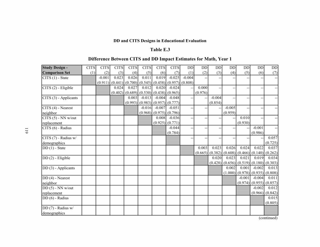
CITS CITS CITS CITS CITS CITS CITS DD DD DD DD DD DD DD(1) (2) (3) (4) (5) (6) (7) (1) (2) (3) (4) (5) (6) (7)
-0.001 0.023 0.026 0.011 0.019 -0.025 -0.004 -- -- -- -- -- --(0.911) (0.441) (0.700) (0.545) (0.458) (0.957) (0.808)
0.024 0.027 0.012 0.020 -0.024 -- 0.000 -- -- -- -- --(0.402) (0.689) (0.530) (0.438) (0.965) (0.976)
0.003 -0.013 -0.004 -0.048 -- -- -0.004 -- -- -- --(0.993) (0.983) (0.957) (0.777) (0.854)
-0.016 -0.007 -0.051 -- -- -- -0.005 -- -- --(0.968) (0.975) (0.796) (0.959)
0.008 -0.036 -- -- -- -- 0.010 -- --(0.925) (0.771) (0.930)
-0.044 -- -- -- -- -- -0.001 --(0.784) (0.986)
-- -- -- -- -- -- 0.057(0.725)
0.003 0.023 0.026 0.024 0.022 0.037(0.665) (0.382) (0.608) (0.466) (0.140) (0.262)
0.020 0.023 0.021 0.019 0.034(0.428) (0.656) (0.519) (0.180) (0.303)
0.002 0.001 -0.002 0.013(1.000) (0.978) (0.935) (0.808)
-0.001 -0.004 0.011(0.974) (0.955) (0.857)
-0.002 0.012(0.966) (0.842)
0.015(0.805)
(continued)
DD (4) - Nearest neighbor
Study Design - Comparison SetCITS (1) - State
CITS (2) - Eligible
CITS (3) - Applicants
CITS (4) - Nearest neighborCITS (5) - NN w/out replacementCITS (6) - Radius
DD (7) - Radius w/ demographics
DD (6) - Radius
DD (5) - NN w/out replacement
Difference Between CITS and DD Impact Estimates for Math, Year 1
DD and CITS Designs in Educational Evaluation
Table E.3
CITS (7) - Radius w/ demographicsDD (1) - State
DD (2) - Eligible
DD (3) - Applicants
119

-- = Not applicable because both the study design and the comparison group selection method are different.
NOTES: The value in the first row of each cell is the estimated difference (in effect size) between impact estimates based on the actual data. The difference in (Row X, Column Y) is equal to the estimated impact based on the comparison group in (Row X) minus the estimated impact based on the group in (Column Y). Effect sizes are calculated using a standard deviation of 21.06, which is the student-level standard deviation for scores in NCEs. The value in the second row of each cell is the p-value for the difference between impact estimates, based on bootstrapped samples (1,000 iterations).
Table E.3 (continued)
120
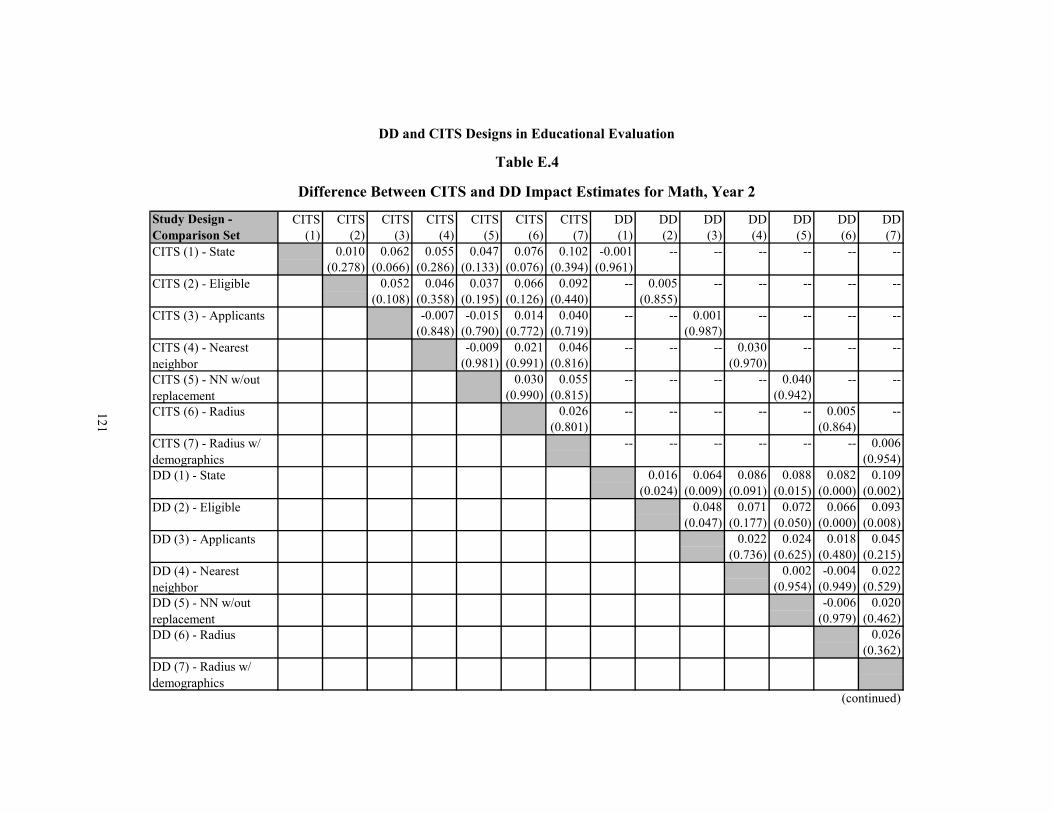
CITS CITS CITS CITS CITS CITS CITS DD DD DD DD DD DD DD(1) (2) (3) (4) (5) (6) (7) (1) (2) (3) (4) (5) (6) (7)
0.010 0.062 0.055 0.047 0.076 0.102 -0.001 -- -- -- -- -- --(0.278) (0.066) (0.286) (0.133) (0.076) (0.394) (0.961)
0.052 0.046 0.037 0.066 0.092 -- 0.005 -- -- -- -- --(0.108) (0.358) (0.195) (0.126) (0.440) (0.855)
-0.007 -0.015 0.014 0.040 -- -- 0.001 -- -- -- --(0.848) (0.790) (0.772) (0.719) (0.987)
-0.009 0.021 0.046 -- -- -- 0.030 -- -- --(0.981) (0.991) (0.816) (0.970)
0.030 0.055 -- -- -- -- 0.040 -- --(0.990) (0.815) (0.942)
0.026 -- -- -- -- -- 0.005 --(0.801) (0.864)
-- -- -- -- -- -- 0.006(0.954)
0.016 0.064 0.086 0.088 0.082 0.109(0.024) (0.009) (0.091) (0.015) (0.000) (0.002)
0.048 0.071 0.072 0.066 0.093(0.047) (0.177) (0.050) (0.000) (0.008)
0.022 0.024 0.018 0.045(0.736) (0.625) (0.480) (0.215)
0.002 -0.004 0.022(0.954) (0.949) (0.529)
-0.006 0.020(0.979) (0.462)
0.026(0.362)
(continued)
DD (4) - Nearest neighbor
Study Design - Comparison SetCITS (1) - State
CITS (2) - Eligible
CITS (3) - Applicants
CITS (4) - Nearest neighborCITS (5) - NN w/out replacementCITS (6) - Radius
DD (7) - Radius w/ demographics
DD (6) - Radius
DD (5) - NN w/out replacement
Difference Between CITS and DD Impact Estimates for Math, Year 2
DD and CITS Designs in Educational Evaluation
Table E.4
CITS (7) - Radius w/ demographicsDD (1) - State
DD (2) - Eligible
DD (3) - Applicants
121
-- = Not applicable because both the study design and the comparison group selection method are different.
NOTES: The value in the first row of each cell is the estimated difference (in effect size) between impact estimates based on the actual data. The difference in (Row X, Column Y) is equal to the estimated impact based on the comparison group in (Row X) minus the estimated impact based on the group in (Column Y). Effect sizes are calculated using a standard deviation of 21.06, which is the student-level standard deviation for scores in NCEs. The value in the second row of each cell is the p-value for the difference between impact estimates, based on bootstrapped samples (1,000 iterations).
Table E.4 (continued)
122

Study Design - Comparison Group CITS (1) CITS (2) CITS (3) CITS (4) CITS (5) CITS (6) CITS (7) DD (1) DD (2) DD (3) DD (4) DD (4) DD (5) DD (6)0.262 0.258 0.253 0.222 0.289 0.344 0.086 0.355 0.346 0.324 0.237 0.307 0.322 0.2470.341 0.349 0.368 0.235 0.338 0.388 0.180 0.431 0.440 0.473 0.343 0.422 0.458 0.3341.000 0.982 0.799 0.430 0.575 0.714 0.276 0.896 -- -- -- -- -- --1.000 0.989 0.870 0.412 0.564 0.641 0.379 0.896
1.000 0.818 0.420 0.572 0.723 0.284 -- 0.894 -- -- -- -- --1.000 0.881 0.409 0.564 0.640 0.379 0.893
1.000 0.344 0.477 0.611 0.211 -- -- 0.907 -- -- -- --1.000 0.358 0.504 0.587 0.357 0.879
1.000 0.774 0.625 0.182 -- -- -- 0.316 -- -- --1.000 0.750 0.653 0.234 0.313
1.000 0.734 0.244 -- -- -- -- 0.488 -- --1.000 0.694 0.281 0.526
1.000 0.296 -- -- -- -- -- 0.754 --1.000 0.320 0.752
1.000 -- -- -- -- -- -- 0.2541.000 0.286
1.000 0.983 0.815 0.504 0.635 0.806 0.5641.000 0.989 0.886 0.644 0.752 0.880 0.616
1.000 0.829 0.496 0.632 0.816 0.5701.000 0.893 0.644 0.755 0.891 0.617
1.000 0.410 0.552 0.709 0.4621.000 0.585 0.702 0.800 0.567
1.000 0.762 0.613 0.3521.000 0.824 0.705 0.468
1.000 0.725 0.4391.000 0.800 0.518
1.000 0.5571.000 0.603
1.0001.000
(continued)
CITS (3) - Applicants
CITS (4) - Nearest neighbor
CITS (5) - NN w/out replacement
CITS (6) - Radius
DD (2) - Eligible
CITS (7) - Radius w/ demographics
DD (1) - State
DD (3) - Applicants
DD (4) - Nearest neighbor
DD (5) - NN w/out replacement
DD (6) - Radius
DD (7) - Radius w/ demographics
CITS (2) - Eligible
DD and CITS Designs in Educational Evaluation
Table E.5
Correlations Between Impact Estimates for Reading (Year 1 and Year 2)
RDD
CITS (1) - State
123
Table E.5 (continued)
NOTES: Values in the table are the correlation between impact estimates, across bootstrapped samples (1,000 iterations). The first row in each cell is the correlation for impacts in Year 1, and the second row is the correlation for impacts in in Year 2. -- = Not applicable because both the study design and the comparison group selection method are different.
124

Study Design - Comparison Group CITS (1) CITS (2) CITS (3) CITS (4) CITS (5) CITS (6) CITS (7) DD (1) DD (2) DD (3) DD (4) DD (4) DD (5) DD (6)0.246 0.239 0.265 0.219 0.252 0.304 0.130 0.340 0.333 0.371 0.202 0.263 0.321 0.3090.216 0.219 0.204 0.244 0.316 0.369 0.165 0.335 0.337 0.360 0.261 0.332 0.418 0.3511.000 0.980 0.792 0.473 0.614 0.754 0.267 0.884 -- -- -- -- -- --1.000 0.981 0.829 0.355 0.489 0.559 0.194 0.851
1.000 0.813 0.475 0.621 0.760 0.265 -- 0.883 -- -- -- -- --1.000 0.846 0.356 0.494 0.569 0.204 0.852
1.000 0.374 0.489 0.618 0.211 -- -- 0.885 -- -- -- --1.000 0.296 0.410 0.473 0.176 0.845
1.000 0.777 0.641 0.192 -- -- -- 0.345 -- -- --1.000 0.744 0.630 0.165 0.288
1.000 0.732 0.193 -- -- -- -- 0.551 -- --1.000 0.671 0.158 0.492
1.000 0.275 -- -- -- -- -- 0.844 --1.000 0.276 0.767
1.000 -- -- -- -- -- -- 0.2751.000 0.284
1.000 0.983 0.801 0.609 0.729 0.893 0.7521.000 0.981 0.832 0.522 0.678 0.868 0.635
1.000 0.816 0.603 0.731 0.899 0.7571.000 0.841 0.524 0.686 0.877 0.640
1.000 0.491 0.617 0.751 0.6091.000 0.458 0.597 0.753 0.565
1.000 0.791 0.658 0.4841.000 0.786 0.616 0.406
1.000 0.780 0.5961.000 0.763 0.527
1.000 0.7691.000 0.672
1.0001.000
(continued)
CITS (3) - Applicants
CITS (4) - Nearest neighbor
CITS (5) - NN w/out replacement
CITS (6) - Radius
DD (2) - Eligible
CITS (7) - Radius w/ demographics
DD (1) - State
DD (3) - Applicants
DD (4) - Nearest neighbor
DD (5) - NN w/out replacement
DD (6) - Radius
DD (7) - Radius w/ demographics
CITS (2) - Eligible
DD and CITS Designs in Educational Evaluation
Table E.6
Correlations Between Impact Estimates for Math (Year 1 and Year 2)
RDD
CITS (1) - State
125
-- = Not applicable because both the study design and the comparison group selection method are different.
NOTES: Values in the table are the correlation between impact estimates, across bootstrapped samples (1,000 iterations). The first row in each cell is the correlation for impacts in Year 1, and the second row is the correlation for impacts in in Year 2.
Table E.6 (continued)
126
Appendix F
Propensity-Score Matching Versus Direct Matching

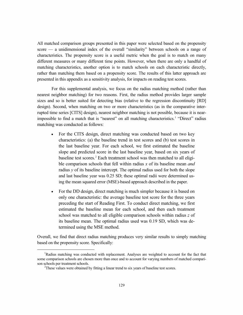
129
All matched comparison groups presented in this paper were selected based on the propensity score — a unidimensional index of the overall “similarity” between schools on a range of characteristics. The propensity score is a useful metric when the goal is to match on many different measures or many different time points. However, when there are only a handful of matching characteristics, another option is to match schools on each characteristic directly, rather than matching them based on a propensity score. The results of this latter approach are presented in this appendix as a sensitivity analysis, for impacts on reading test scores.
For this supplemental analysis, we focus on the radius matching method (rather than nearest neighbor matching) for two reasons. First, the radius method provides larger sample sizes and so is better suited for detecting bias (relative to the regression discontinuity [RD] design). Second, when matching on two or more characteristics (as in the comparative inter-rupted time series [CITS] design), nearest neighbor matching is not possible, because it is near-impossible to find a match that is “nearest” on all matching characteristics.1 “Direct” radius matching was conducted as follows:
• For the CITS design, direct matching was conducted based on two key characteristics: (a) the baseline trend in test scores and (b) test scores in the last baseline year. For each school, we first estimated the baseline slope and predicted score in the last baseline year, based on six years of baseline test scores.2 Each treatment school was then matched to all eligi-ble comparison schools that fell within radius x of its baseline mean and radius y of its baseline intercept. The optimal radius used for both the slope and last baseline year was 0.25 SD; these optimal radii were determined us-ing the mean squared error (MSE)-based approach described in the paper.
• For the DD design, direct matching is much simpler because it is based on only one characteristic: the average baseline test score for the three years preceding the start of Reading First. To conduct direct matching, we first estimated the baseline mean for each school, and then each treatment school was matched to all eligible comparison schools within radius z of its baseline mean. The optimal radius used was 0.19 SD, which was de-termined using the MSE method.
Overall, we find that direct radius matching produces very similar results to simply matching based on the propensity score. Specifically:
1Radius matching was conducted with replacement. Analyses are weighted to account for the fact that some comparison schools are chosen more than once and to account for varying numbers of matched compari-son schools per treatment schools.
2These values were obtained by fitting a linear trend to six years of baseline test scores.

130
• Table F.1 presents the characteristics of schools in the “radius” and “radius
direct” comparison sets. The results show that the latter comparison sets are similar to the Reading First schools; they differ by no more than 0.25 SD on test scores and demographic characteristics.
• Table F.2 shows the amount of overlap between the comparison schools se-lected using propensity-based radius matching and direct radius matching. There is substantial overlap between the two methods, especially among sets used in the DD analysis (based on three years of baseline test scores).
• Figure F.1 plots the third-grade test scores of schools in the comparison set created using “direct” radius matching. For reference, the test scores of schools in the comparison set created using propensity-based radius match-ing are also shown. Both sets have a similar baseline trend as the Reading First schools.
• Figures F.2 and F.3 show the estimated impact of Reading First based on the “radius direct” comparison set, for the CITS and DD designs, respectively. As a reference point, the RD impact estimate (the benchmark) and the pro-pensity-based radius estimates are also shown. As seen here, the propensity-based and direct radius matching methods produce similar findings.
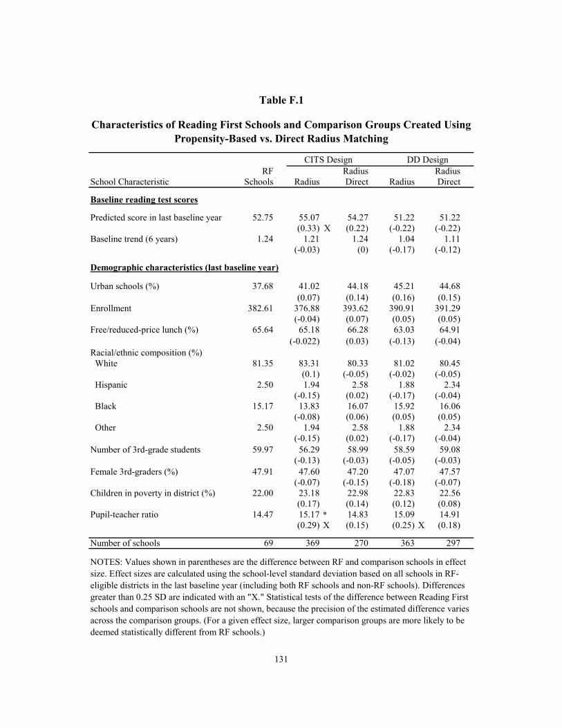
131
RF Radius RadiusSchool Characteristic Schools Radius Direct Radius Direct
Baseline reading test scores
Predicted score in last baseline year 52.75 55.07 54.27 51.22 51.22(0.33) X (0.22) (-0.22) (-0.22)
Baseline trend (6 years) 1.24 1.21 1.24 1.04 1.11(-0.03) (0) (-0.17) (-0.12)
Demographic characteristics (last baseline year)
Urban schools (%) 37.68 41.02 44.18 45.21 44.68(0.07) (0.14) (0.16) (0.15)
Enrollment 382.61 376.88 393.62 390.91 391.29(-0.04) (0.07) (0.05) (0.05)
Free/reduced-price lunch (%) 65.64 65.18 66.28 63.03 64.91(-0.022) (0.03) (-0.13) (-0.04)
Racial/ethnic composition (%) White 81.35 83.31 80.33 81.02 80.45
(0.1) (-0.05) (-0.02) (-0.05) Hispanic 2.50 1.94 2.58 1.88 2.34
(-0.15) (0.02) (-0.17) (-0.04) Black 15.17 13.83 16.07 15.92 16.06
(-0.08) (0.06) (0.05) (0.05) Other 2.50 1.94 2.58 1.88 2.34
(-0.15) (0.02) (-0.17) (-0.04)Number of 3rd-grade students 59.97 56.29 58.99 58.59 59.08
(-0.13) (-0.03) (-0.05) (-0.03)Female 3rd-graders (%) 47.91 47.60 47.20 47.07 47.57
(-0.07) (-0.15) (-0.18) (-0.07)Children in poverty in district (%) 22.00 23.18 22.98 22.83 22.56
(0.17) (0.14) (0.12) (0.08)Pupil-teacher ratio 14.47 15.17 * 14.83 15.09 14.91
(0.29) X (0.15) (0.25) X (0.18)
Number of schools 69 369 270 363 297
CITS Design DD Design
NOTES: Values shown in parentheses are the difference between RF and comparison schools in effect size. Effect sizes are calculated using the school-level standard deviation based on all schools in RF-eligible districts in the last baseline year (including both RF schools and non-RF schools). Differences greater than 0.25 SD are indicated with an "X." Statistical tests of the difference between Reading First schools and comparison schools are not shown, because the precision of the estimated difference varies across the comparison groups. (For a given effect size, larger comparison groups are more likely to be deemed statistically different from RF schools.)
Table F.1
Characteristics of Reading First Schools and Comparison Groups Created Using Propensity-Based vs. Direct Radius Matching
132
CITS DDCITS Radius DD Radius
Among schools in the following Radius Direct Radius Directcomparison groups… (N) (369) (270) (363) (297)
CITS - Radius (369) 100% 70% 94% 77%CITS - Radius direct (270) 96% 100% 99% 85%DD - Radius (363) 95% 73% 100% 79%DD - Radius direct (297) 95% 77% 97% 100%
Overlap Between Comparison Groups Created Using Propensity-Based Radius Matching vs. Direct Radius Matching, for Impacts
on Reading
… Percentage that are also in …
NOTES: Value in (Row X, Column Y) = Percentage of schools in the comparison group in Row X that are also part of the comparison group in Column Y.(N) = Sample size of comparison group.
Table F.2
DD and CITS Designs in Educational Evaluation

133
0
10
20
30
40
50
60
-5 -4 -3 -2 -1 0 1 2
3rd-
grad
e re
adin
g te
st sc
ores
(NC
Es)
Relative year (Last baseline = 0)
DD and CITS Designs in Educational Evaluation
Figure F.1
Reading Test Score Trends for Reading First Schools and Comparison Groups Created Using Propensity-Based Radius Matching vs. Direct Radius
Matching
RF schools (N = 69)
Radius (N = 393)
Radius direct (N = 270)
0
10
20
30
40
50
60
-5 -4 -3 -2 -1 0 1 2
3rd-
grad
e re
adin
g te
st sc
ores
(NC
Es)
Relative year (Last baseline = 0)
B. Matched groups for DD design
RF schools (N = 69)
Radius (N = 363)
Radius direct (N = 327)
Reading First begins
A. Matched groups for CITS design

134
-0.026 -0.023-0.038
-0.20
-0.15
-0.10
-0.05
0.00
0.05
0.10
0.15
0.20
0.25
RD design (N = 99; SE =0.075; p = 0.725)
Radius (N = 369; SE =0.025; p = 0.358)
Radius direct (N = 270; SE= 0.028; p = 0.185)
Effe
ct si
ze
DD and CITS Designs in Educational Evaluation
Figure F.2
Estimated Impact on Reading Scores, CITS DesignBased on Propensity-Based Radius Matching vs. Direct Radius Matching
(N = number of comparison schools, SE = standard error, p = p-value)
Year 1
0.057
-0.008 0.005
-0.25-0.20-0.15-0.10-0.050.000.050.100.150.200.25
RD design (N = 99; SE =0.072; p = 0.434)
Radius (N = 369; SE =0.028; p = 0.781)
Radius direct (N = 270; SE= 0.032; p = 0.863)
Effe
ct si
ze
Year 2

135
-0.026 -0.031 -0.020
-0.20
-0.15
-0.10
-0.05
0.00
0.05
0.10
0.15
0.20
0.25
RD design (N = 99; SE =0.075; p = 0.725)
Radius (N = 363; SE =0.023; p = 0.177)
Radius direct (N = 297; SE= 0.025; p = 0.418)
Effe
ct si
ze
DD and CITS Designs in Educational Evaluation
Figure F.3
Estimated Impact on Reading Scores, DD DesignBased on Propensity-Based Radius Matching vs. Direct Radius Matching
(N = number of comparison schools, SE = standard error, p = p-value)
Year 1
0.057
-0.0120.011
-0.25
-0.20
-0.15
-0.10
-0.05
0.00
0.05
0.10
0.15
0.20
0.25
RD design (N = 99; SE =0.072; p = 0.434)
Radius (N = 363; SE =0.023; p = 0.588)
Radius direct (N = 297; SE= 0.025; p = 0.67)
Effe
ct si
ze
Year 2

137
References
Allison, P. 2001. Missing Data. Thousand Oaks, CA: Sage.
Bell, S. H., and L. L. Orr. 1995. “Are Nonexperimental Estimates Close Enough for Policy Purposes? A Test for Selection Bias Using Experimental Data.” Proceedings of the American Statistical Association 228-233.
Bertrand, M., E. Duflo, and S. Mullainathan. 2002. “How Much Should We Trust Difference-in-Difference Estimates?” NBER Working Paper, 8841. Cambridge, MA: National Bureau of Economic Research.
Bloom, H. S. 1999. Estimating Program Impacts on Student Achievement Using “Short” Interrupted Time Series. MDRC Working Paper on Research Methodology. New York: MDRC.
Bloom, H. S. 2003. “Using ‘Short’ Interrupted Time-Series Analysis to Measure the Impacts of Whole-School Reforms: With Applications to a Study of Accelerated Schools.” Evaluation Review 27 (3): 3-49.
Bloom, H. S. 2012. “Modern Regression Discontinuity Analysis.” Journal of Research on Educational Effectiveness 5 (1): 43-82.
Bloom, H. S., C. Michalopolous, and C. J. Hill. 2005. “Using Experiments to Assess Nonexperimental Comparison-Group Methods for Measuring Program Effects. Pages 173-235 in H. S. Bloom (ed.), Learning More from Social Experiments: Evolving Analytical Approaches. New York: Russell Sage.
Bloom, H. S., and J. A. Riccio. 2005. “Using Place-Based Random Assignment and Comparative Interrupted Time-Series Analysis to Evaluate the Jobs-Plus Employment Program for Public Housing Residents.” Annals of the American Academy of Political and Social Science 599 (1): 19-51.
Cochran, W. G., and D. B. Rubin. “Controlling Bias in Observational Studies: A Review.” Sankhya: The Indian Journal of Statistics (Series A) 35: 417-446.
Cook, T. D. 2008. “Waiting for Life to Arrive: A History of the Regression-Discontinuity Design in Psychology, Statistics and Economics.” Journal of Econometrics 142: 636-654.
Cook, T. D., W. R. Shadish, and V. C. Wong. 2008. “Three Conditions Under Which Experiments and Observational Studies Produce Comparable Causal Estimates: New Findings from Within-Study Comparisons.” Journal of Policy Analysis and Management 27 (4): 724-750.
Dee, T. S., and B. A. Jacob. 2011. “The Impact of No Child Left Behind on Student Achievement.” Journal of Policy Analysis and Management 30 (3): 418-446.
Diaz, J. J., and S. Handa. 2006. An Assessment of Propensity Score Matching as a Nonexperimental Impact Estimator. Journal of Human Resources 41 (2): 319-345.

138
Fortson, K., N. Verbitsky-Savitz, E. Kopa, and P. Gleason. 2012. Using an Eperimental Evaluation of Charter Schools to Test Whether Nonexperimental Comparison Group Methods Can Replicate Experimental Impact Estimates (NCEE Technical Methods Report 2012-4019). Washington, DC: National Center for Education Evaluation and Regional Assistance, Institute of Education Sciences, U.S. Department of Education.
Gamse, B. C., R. T. Jacob, M. Horst, B. Boulay, and F. Unlu. 2008. Reading First Impact Study Final Report (NCEE 2009-4038). Washington, DC: National Center for Education Evaluation and Regional Assistance, Institute of Education Sciences, U.S. Department of Education.
Glazerman, S., D., M. Levy, and D. Myers. 2003. “Nonexperimental Versus Experimental Estimates of Earnings Impacts.” Annals of the American Academy of Political and Social Science 589 (1): 63-93.
Gu, C., and P. R. Rosenbaum. 1993. “Comparison of Multivariate Matching Methods: Structures, Distances and Algorithms.” Journal of Computational and Graphical Statistics 2: 405-420.
Hansen, B. B. 2004. “Full Matching in an Observational Study of Coaching for the SAT.” Journal of the American Statistical Association 99 (467): 609-618.
Heckman, J., H. Ichimura, J. C. Smith, and P. Todd. 1998. “Characterizing Selection Bias.” Econometrika 66: 1017-1098.
Heckman, J., H. Ichimura, and P. E. Todd. 1997. “Matching as an Econometric Evaluation Estimator: Evidence from Evaluating a Job Training Program.” Review of Economic Studies 64: 605-654.
Heckman, J., R. LaLonde, and J. Smith. 1999. “The Economics and Econometrics of Active Labor Market Programs.” Pages 1865-2073 in O. Ashenfelter and D. Card (eds.), Handbook of Labor Economics (Vol. 4). Amsterdam, Netherlands: Elsevier Science.
Heckman, J., and J. A. Smith. 1999. “The Pre-Program Earnings Dip and the Determinants of Participation in a Social Program: Implication for Simple Program Evaluation Strategies.” Economic Journal 109: 313-348.
Herlihy, C. M., and J. J. Kemple. 2004. The Talent Development Middle School Model: Context, Components, and Initial Impacts on Students’ Performance and Attendance. New York: MDRC.
Ho, D., K. Imai, G. King, and E. A. Stuart. 2007. “Matching as Nonparametric Preprocessing for Reducing Model Dependence in Parametric Causal Inference. Political Analysis 15 (3): 199-236.
Imbens, G. W., and K. Kalyanaraman. 2009. “Optimal Bandwidth Choice for the Regression Discontinuity Estimator.” Unpublished working paper.
Jacob, R. T., P. Zhu, M-A. Somers, and H. S. Bloom. 2012. A Practical Guide to Regression Discontinuity. MDRC Working Paper. New York: MDRC.
139
Kemple, J. J., C. M. Herlihy, and T. J. Smith. 2005. Making Progress Toward Graduation: Evidence from the Talent Development High School Model. New York: MDRC.
Lee, D., and T. Lemieux. 2010. “Regression Discontinuity Designs in Economics.” Journal of Economic Literature 48: 281-355.
McCrary, J. 2008. “Manipulation of the Running Variable in the Regression Discontinuity Design: A Density Test.” Journal of Econometrics 142 (2): 698-714.
Meyer, B. D. 1995. “Natural and Quasi-Experiments in Economics.” Journal of Business and Economic Statistics 13 (2): 151-161.
Orr, L. L., S. H. Bell, and R. Kornfeld. 2004. Tests of Nonexperimental Methods for Evaluating the Impact of the New Deal for Disabled People (NDDP). Sheffield, UK: Department for Work and Pensions.
Quint, J., H. S. Bloom, A. R. Black, and L. Stephens. 2005. The Challenge of Scaling Up Educational Reform: Findings and Lessons from First Things First. New York: MDRC.
Rosenbaum, P. R. 1989. “Optimal Matching for Observational Studies.” Journal of the American Statistical Association, 84 (408): 1024-1032.
Rosenbaum, P. R., and D. B. Rubin. 1983. “The Central Role of the Propensity Score in Observational Studies for Causal Effects.” Biometrika 70: 41-55.
Rubin, D. B. 2001. “Using Propensity Scores to Help Design Observational Studies: Application to the Tobacco Litigation.” Health Services and Outcomes Research Methodology 2 (3-4): 169-188.
Schochet, P. 2008. Statistical Power for Regression Discontinuity Designs in Education Evaluations (Technical Methods Report NCEE 2008-4026). Washington, DC: National Center for Education Evaluation and Regional Assistance, Institute of Education Sciences, U.S. Department of Education.
Shadish, W. R., T. D. Cook, and D. T. Campbell. 2002. Experimental and Quasi-Experimental Designs for Generalized Causal Inference. New York: Houghton Mifflin.
Snipes, J. C., G. I. Holton, F. Doolittle, and L. Sztejnberg. 2006. Striving for Student Success: The Effect of Project GRAD on High School Student Outcomes in Three Urban School Districts. New York: MDRC.
Sparks, S. D. 2010.“ ‘What Works’ Broadens Its Research Standards: Clearinghouse Moves Past ‘Gold Standard.’ ” Education Week ( Oct. 20). Web site:
http://www.edweek.org/ew/articles/2010/10/20/08wwc.h30.html.
Steiner, P. M., T. D. Cook, W. R. Shadish, and M. H. Clark. 2010. “The Importance of Covariate Selection in Controlling for Selection Bias in Observational Studies.” Psychological Methods 15 (3): 250-267.
140
Thistlethwaite, D., and D. Campbell. 1960. “Regression-Discontinuity Analysis: An Alternative to the Ex Post Facto Experiment.” Journal of Educational Psychology 51: 309-317.
Wing, C., and T. D. Cook. 2013. “Strengthening the Regression Discontiuity Design Using Additional Design Elements: A Within-Study Comparison.” Manuscript under review.
Wong, M., T. D. Cook, and P. M. Steiner. 2011. “No Child Left Behind: An Interim Evaluation of Its Effects on Learning Using Two Interrupted Time Series Each With Its Own Non-Equivalent Comparison Series.” Northwestern University Institute for Policy Research Working Paper Series, WP 09-11. Evanston, IL: Northwestern University Institute for Policy Research.

About MDRC
MDRC is a nonprofit, nonpartisan social and education policy research organization dedicated to learning what works to improve the well-being of low-income people. Through its research and the active communication of its findings, MDRC seeks to enhance the effectiveness of so-cial and education policies and programs.
Founded in 1974 and located in New York City and Oakland, California, MDRC is best known for mounting rigorous, large-scale, real-world tests of new and existing policies and programs. Its projects are a mix of demonstrations (field tests of promising new program approaches) and evaluations of ongoing government and community initiatives. MDRC’s staff bring an unusual combination of research and organizational experience to their work, providing expertise on the latest in qualitative and quantitative methods and on program design, development, implementa-tion, and management. MDRC seeks to learn not just whether a program is effective but also how and why the program’s effects occur. In addition, it tries to place each project’s findings in the broader context of related research — in order to build knowledge about what works across the social and education policy fields. MDRC’s findings, lessons, and best practices are proac-tively shared with a broad audience in the policy and practitioner community as well as with the general public and the media.
Over the years, MDRC has brought its unique approach to an ever-growing range of policy are-as and target populations. Once known primarily for evaluations of state welfare-to-work pro-grams, today MDRC is also studying public school reforms, employment programs for ex-offenders and people with disabilities, and programs to help low-income students succeed in college. MDRC’s projects are organized into five areas:
• Promoting Family Well-Being and Children’s Development
• Improving Public Education
• Raising Academic Achievement and Persistence in College
• Supporting Low-Wage Workers and Communities
• Overcoming Barriers to Employment
Working in almost every state, all of the nation’s largest cities, and Canada and the United Kingdom, MDRC conducts its projects in partnership with national, state, and local govern-ments, public school systems, community organizations, and numerous private philanthropies.