
The Swing Voter’s Curse in the Laboratory - nyu.edu form of the swing voter’s curse that we have...
45
The Swing Voter’s Curse in the Laboratory 1 Marco Battaglini Department of Economics Princeton, NJ 08544-1021 [email protected] Rebecca Morton Department of Politics New York University 726 Broadway, 7th Floor New York, NY 10003 [email protected] Thomas Palfrey Departments of Politics and Economics Princeton, NJ 08544-1021 [email protected] December 21, 2005. 1 This research was supported by the Princeton Laboratory for Experimental Social Science (PLESS). The financial support of the National Science Foundation is gratefully acknowledged by Battaglini (SES-0418150) and Palfrey (SBR-0098400 and SES-0079301). We thank Karen Kaiser and Stephanie Wang for research assistance, and Stephen Coate for comments.
Transcript of The Swing Voter’s Curse in the Laboratory - nyu.edu form of the swing voter’s curse that we have...
The Swing Voter’s Curse in the Laboratory1
Marco BattagliniDepartment of EconomicsPrinceton, NJ [email protected]
Rebecca MortonDepartment of PoliticsNew York University
726 Broadway, 7th FloorNew York, NY 10003
Thomas PalfreyDepartments of Politics and Economics
Princeton, NJ [email protected]
December 21, 2005.
1This research was supported by the Princeton Laboratory for Experimental Social Science(PLESS). The financial support of the National Science Foundation is gratefully acknowledgedby Battaglini (SES-0418150) and Palfrey (SBR-0098400 and SES-0079301). We thank KarenKaiser and Stephanie Wang for research assistance, and Stephen Coate for comments.

Abstract
This paper reports the first laboratory study of the swing voter’s curse and providesinsights on the larger theoretical and empirical literature on "pivotal voter" models. Ourexperiment controls for different information levels of voters, as well as the size of theelectorate, the distribution of preferences, and other theoretically relevant parameters.The design varies the share of partisan voters and the prior belief about a payoff relevantstate of the world. Our results support the equilibrium predictions of the Feddersen-Pesendorfer model, and clearly reject the notion that voters in the laboratory use naivedecision-theoretic strategies. The voters act as if they are aware of the swing voter’s curseand adjust their behavior to compensate. While the compensation is not complete andthere is some heterogeneity in individual behavior, we find that aggregate outcomes, suchas efficiency, turnout, and margin of victory, closely track the theoretical predictions.

I Introduction
Voter turnout has traditionally proven to be a difficult phenomenon to explain. Rational
models highlight the fact that the incentives to participate in an election depend on the
probability of being pivotal. If voting is costly, then significant turnout in large elections
is inconsistent with equilibrium behavior.1 If voting is costless, then abstention is a
dominated choice. However, this is also inconsistent with observed voting behavior.
Voters often selectively abstain in the same election—Timothy Feddersen and Wolfgang
Pesendorfer [1996] report that almost 1 million voters chose to vote in the 1994 Illinois
gubernatorial contest but abstained on the state constitutional amendment listed on the
same ballot, even though the constitutional amendment was listed first on the ballot. W.
Mark Crain, Donald R. Leavens, and Lynn Abbot [1987] report that in the 1982 midterm
elections Congressional district turnout levels averaged 3% higher for the Senate contests
in those states with such contests than the House races that were on the same ballot.
In seven of the 219 contests they studied the difference in turnout was larger than the
margin of victory in the House race, suggesting that voters were abstaining even in close
House contests.2 Assuming that voting is virtually costless when already in the ballot
booth, this would seem to be irrational.
Feddersen and Pesendorfer [1996] show that these large abstention rates can be ex-
plained even if the cost of voting is zero if there is asymmetric information, thereby
rationalizing such behavior. They draw an analogy between voters’ problem and the
“winner’s curse” observed among bidders in an auction (see John Kagel and Dan Levin
[2005] and Richard Thaler [1996]). A poorly informed voter may be better off in equi-
librium to leave the decision to the informed voters because his uninformed vote may go
against the choice of better informed voters, and could even decide the outcome in the
wrong direction. The voter, therefore, may rationally “delegate” the decision to more
informed voters by abstaining even if voting is costless. Feddersen and Pesendorfer [1996]
name this phenomenon the Swing Voter’s Curse.
This paper reports the first laboratory study of the swing voter’s curse. Our results,
however, provide insights on the larger “pivotal-voter” literature. This literature includes
the earlier models with symmetric information and costly voting (Ledyard [1984], Palfrey
1See John Ledyard [1984] and Thomas Palfrey and Howard Rosenthal [1983, 1985].2They omitted states with gubernatorial contests to focus on the choice whether to vote in both the
Senate and House races. Martin Wattenberg, Ian McAllister, and Anthony Salvanto [2000] report thatin the 1994 California election 8% of those who voted for governor abstained in state legislative electionsand over 35% abstained on state supreme court judicial retention votes. They note that the pattern ofabstention appears independent of ballot order, with the abstention of those who voted in the governors’race only 2% on two ballot propositions which were seven ballot positions below the judicial retentionelections.
1

and Rosenthal [1983]); asymmetric information and costly voting Palfrey and Rosenthal
[1985]); and the broader theoretical literature that focuses on information aggregation
in elections with common or private values and asymmetric information (David Austen-
Smith and Jeffrey Banks [1996], Marco Battaglini [2005], Feddersen and Pesendorfer [1997,
1999] and others).
This theory explains some empirical facts, but it remains —along with rational theories
of voting more generally—highly controversial.3 Empirical evidence has been produced
both in favor and against rational voter theories, especially when compared to the as-
sumption that voters act naively and ignore strategic considerations.4 None of these
results, however, are conclusive, partly because field data sets are not rich enough to
identify all the variables that may affect voters decisions. This is especially true for tests
of rational theories of voting based on asymmetric information, such as the Swing Voter’s
Curse.
To overcome these problems, we design a laboratory experiment that provides a sharp
test of the theoretical predictions of the Feddersen-Pesendorfer model. The laboratory
setting allows us to control and directly observe the level of information of different voters,
as well as preferences, voting costs, and other theoretically relevant parameters.
As in Feddersen and Pesendorder [1996], we assume two possible states of the world, A
and B; and two policies: a status quo, and a new proposal. Preferences in the electorate
are heterogeneous. There are independent voters who would like to vote for the status
quo in state A, and for the new proposal in state B. There are also partisans who always
prefer the status quo regardless of the state. A fraction of the independent voters can
be informed on the state of the world, the remaining fraction receives no information.
To focus on the incentive to abstain even when voting is costless, we assume zero cost
of voting. The goal of the model is to provide a framework to test the swing voter’s
curse by studying the behavior of independent voters, and more generally the predictive
abilities of informative theories of voting with asymmetric information, heterogeneous
level of information and preferences.
To this goal, we consider a two dimensional design which allows to test the effect of
variations in the share of partisan voters and the prior probability of the states on the
voting equilibrium. First we consider the case in which the states are equally likely. In this
3See Feddersen [2004] for a recent discussion.4Feddersen [2004] reviews this literature. John Matsusaka and Filip Palda [1999], based on an extensive
study of turnout decisions using both survey and aggregate data, contend that theories of voter turnoutprovide little explanatory power in explaining voter choices and that turnout decisions appear to berandom. Stephen Coate, John Conlin, and Andrea Moro [2005] provide evidence that a simple modelof expressive voting better explains turnout in local Texas elections than the standard model on pivotalvoting.
2
case, if there are no partisans, the model predicts that all uninformed independent should
abstain and “delegate” the choice to informed independent voters. This is a particularly
strong form of the swing voter’s curse that we have described above which implies zero
participation of uniformed voters. As the share of partisans who always vote for the
status quo regardless of the state (which for simplicity we may call policy A, as the
state of the world) is increased, the predictions of the model become less extreme: the
uniformed independents still abstain with positive probability, but with probability that
is decreasing in the share of partisans; moreover when they vote they are expected to
vote for the new proposal (B). This result continues to be true even when the state in
which the status quo is optimal is more likely: therefore creating a situation in which
uninformed independent voters vote against their prior. These predictions of the Nash
equilibrium with rational voters, therefore, are in sharp contrast with the prediction of
a model of expressive voting, in which voters are not voting on the basis of strategic
considerations, but on the basis of the intensity of their preferences as if in a single agent
decision problem.
Our empirical results strongly support the prediction of the Nash equilibrium of the
model, allowing rejecting the assumption that voters are using naive strategies. Not only
the comparative statics is in line with the model, but also the average probability of voting
is consistent with the theoretical prediction.
A common prediction in the literature on voting with asymmetric information is that
elections tend to aggregate information dispersed among voters. The same phenomenon
should be observed in this environment despite the fact that in this model voters do
not have common values: though partisans skew the election toward the status quo,
the uniformed swing voters endogenously vote to offset this bias. We find significant
evidence that uninformed voters do offset the votes of partisans, allowing for information
aggregation close to that possible without partisans.
We also find that as the number of voters who are informed increases both turnout and
the margin of victory increases, as predicted by the theory. We discuss the implications of
the relationship between information, turnout, and victory margins for tests of strategic
voting that focus on the relationship between closeness and turnout levels.
Our attempt to test the pivotal voting model of turnout and behavior using labora-
tory experiments is significantly different from previous experiments which have primarily
focused on cases where information is symmetric and voting is costly.5 Much less exper-
5See Arthur Schram and Joop Sonnemans [1996], Cason and Mui [2005], Grosser, Kugler, and Schram[2005] who have studied strategic voters participation in laboratory experiments, focusing on environmentswith symmetric information and homogeneous costs. One problem with these early works is that,under these assumptions, voting models may have many equilibria. David Levine and Palfrey [2005]have recently conducted expeirments based on a model with heterogeneous costs which has a unique
3

imental work has been done with models with asymmetric information. Serena Guar-
naschelli, Richard McKelvey, and Palfrey [2000] test Feddersen and Pesendorfer Jury’s
model (Feddersen and Pesendorfer [1998]) and focus on information aggregation in small
committees. They rule out abstention by assumption, and therefore do not provide ev-
idence on participation. Moreover, they assume common values, no partisans, and all
voters are equally well informed. Battaglini, Rebecca Morton, and Palfrey [2005] study
sequential voting in a similar model with common values and no partisans. Although
they let voters abstain, in their model all voters receive signals of the same quality, so the
swing voter’s curse can not be observed.
A significant non-experimental empirical literature on turnout exists and a number of
these studies attempt to test the pivotal voter model on large elections or a variant of
the model as augmented by group and/or ethical motivations for voting.6 None of these
studies are able to evaluate the role of asymmetric information in explaining abstention
and test the swing voter’s curse.
A number of researchers have used variations in voter information in field studies to
evaluate the effect of information on the choice to abstain which suggest support for the
swing voter’s curse.7 The main finding is that turnout is positively correlated with voter
information levels, but this work cannot identify the causal relationship since the demand
for political information may be derived from the decision to participate. Recently
researchers have examined the impact on turnout of changes in political information
where political information is arguably an exogenous variable. Monika McDermott [2005]
and David Klein and Lawrence Baum [2001] present evidence that respondents to surveys
during elections are more likely to state preferences when information is provided to them.
Matthew Gentzkow [2005] shows that decreases in voter information associated with the
advent to television in U.S. counties is correlated with decreasing voter turnout. David
Lassen [2005] examined turnout in a Copenhagen election where residents of four of the
city’s fifteen districts were provided with detailed information about the choices in an
upcoming referendum. He finds that voters provided with more information were more
likely to participate.
Lassen argues that there are two possible explanations for the relationship between
equilibrium. They find support for the three primary predictions of the rational model: (1) turnoutdeclines with the size of the electorate (the size effect); (2) turnout is higher in elections that are expectedto be close (the competition effect); and (3) turnout is higher for voters who prefer the less popularalternative (the underdog effect).
6See, for example, Stephen Hansen, Palfrey, and Rosenthal [1987], John Filer, Lawrence Kenny, andMorton [1993], Roni Schachar and Barry Nalebuff [1999], Coate and Conlin [2004], Abdul Noury [2004],and Coate, Conlin, and Moro [2004]).
7See, for example, Palfrey and Keith Poole [1987], Wattenberg, McAllister, and Salvanto [2000], andTom Coupe and Noury [2004].
4
information and turnout—the swing voter’s curse theory of Feddersen and Pesendorfer and
a decision-theoretic model first suggested by Matsusaka [1995] in which voters are more
likely to turnout the more confident they are in the correctness of their choices. Gentzkow
also notes that his results support a number of theories that argue that information
increases turnout including simple decision-theoretic ones as well. Lassen concludes (p.
116): “The natural experiment used here does not allow for distinguishing between the
decision-theoretic and game-theoretic approaches ....; this may call for careful laboratory
experiments, as the predictions of the models differ in only subtle ways that can be difficult
to accomodate in even random social experiments, but the results reported in this article
can serve as a necessary first step in motivating the importance of such experiments ...”
The upshot of these studies is that the available natural experiments cannot analyze
the data to distinguish between these two approaches and we take the next step in the
study of the swing voter’s curse in this paper.8 In our experimental design we are able
to investigate 240 different elections which vary between all voters uninformed to over 70
percent informed. Thus, we can consider the effect of information on aggregate turnout
levels as well as the margin of victory, considerations that are difficult to make using nat-
ural experiments. As noted above, we are able to consider a variety of degrees of partisan
balance and information distribution as well. Finally, we can consider how different in-
dividuals choose depending on the information available and the partisan balance. With
this wide array of observations we can show that the game theoretic model is a better
predictor of behavior than the decision-theoretic approach.
The organization of the reminder of the paper is as follows. In Section I we present the
model. Section II characterizes the equilibrium. Section III describes the experimental
design and the hypotheses to be tested. Section IV presents the experimental results.
Section V concludes. All formal proofs are presented in a technical Appendix at the end
of the paper.
II The Model
We consider a game with a set of N voters who deliberate by majority rule. There are
two alternatives A, B and two states of the world: in the first state A is optimal and in
the second state B is optimal. Without loss of generality, we label A the first state and
B the second.
A number n ≤ N of the voters are independent voters. These voters have identical
preferences represented by a utility function u(x, θ) that is a function of the state of the
8Cross sectional and longitudinal studies have their own methodological shortcomings. See BernardGroffman [1993].
5

world θ ∈ {A,B} and the action x ∈ {A,B}:u(A,A) = u(B,B) = 1
u(A,B) = u(B,A) = 0
State A has a prior probability π ≥ 12. The true state of the world is unknown, but each
voter may receive an informative signal. We assume that signals of different agents are
conditionally independent. The signal can take three values a, b, and φ with probability:
Pr(a |A) = Pr(b |B ) = p and Pr(φ |A) = Pr(φ |B ) = 1− p
The agent, therefore, is perfectly informed on the state of the world with probability p,
and has no information with probability 1− p.
The remaining m = N − n voters are partisan voters. We assume that the partisans
strictly prefer policy A in all states. For convenience we assume that m is even, n is odd
and m ≤ n− 3.9After swing voters have seen their private signal, all voters vote simultaneously. Each
voter can vote for A, vote for B, or abstain. In any equilibrium, the independent voters
who receive an informative signal always strictly prefer the state that matches their signal;
and the partisans always strictly prefer stateA: in any equilibrium, therefore independents
would always vote for the state suggested by their signal, and partisans would always vote
for A. We can therefore focus on the behavior of the uninformed agents. Let σiA, σiB,
and σiφ be respectively the probability that an uninformed agents votes for A, B and
abstains.
An equilibrium of this game is symmetric if agents with the same signal use the same
strategy: σi = σ for all i. We analyze symmetric equilibria in which agents do not use
weakly dominated strategies and we will refer to them simply as equilibria.
III The Voting Equilibrium
In this section we characterize the equilibria of the voting game, and the equilibrium is
unique for the experimental parameters. With respect to Feddersen and Pesendorfer
[1996] and other previous results in the literature, we do not limit the analysis to asymp-
totic results that hold as the size of the electorate grows to infinity, but focus on results
that hold even for a finite number of voters. This allows us to test the model directly
with an electorate of a size that can be managed in a laboratory. Formal proofs of all the
results appear in an Appendix.9These assumptions are made only to simplify the notation. In Feddersen and Pesendorfer [1996] m
is random variable; however, since they focus the analysis on the limit case in which n→∞, the realizedfraction of partisan voters is constant by the Law of Large Numbers in their model.
6
III.1 No Partisan Bias
We first consider the benchmark case in which all the voters have the same common value,
so m = 0.
Lemma 1 Let m = 0. If π = 12, then σA = σB; if π > 1
2, then σA ≥ σB.
The intuition of this result is as follows. If the uniformed voters are voting for, say B,
with higher probability, then if pivotal it is more likely that alternative A has attracted
more votes from informed voters. If this is the case, then conditioning on the pivotal
event, alternative A is more attractive to an uninformed independent, and none of them
would vote for B, a contradiction.
Though this result provides testable predictions, it can be made more precise:
Proposition 1 Let m = 0. If π = 12, then σA = σB = 0; if π > 1
2, then σA ≥ σB = 0.
This is a particular form of the Swing Voters’ Curse. To see the intuition behind it,
suppose the prior is π = 12. If an uninformed voter were to choose in isolation, he would
be indifferent between the two options A or B. When voting in a group, however, he
knows that with positive probability some other voter is informed. By voting, he risks
voting against this more informed voter. So, since he has the same preferences of this
informed voter and he is otherwise indifferent among the alternatives because he has no
private information on the state, he always finds it optimal to abstain. When the prior is
π > 12, the problem of the voter is more complicated. In this case the swing voter’s curse
is mitigated by the fact that the prior favors one of the two alternatives. As before, the
voter does not want to vote against an informed voter. However, he is not sure that there
is an informed voter: and if no informed voter is voting, he strictly prefers alternative A
since this is ex ante more likely. Thus although the voter never finds it optimal to vote
for B, he may find it optimal to vote for A. The higher is π, the higher is the incentive
to vote for A; the higher is p (i.e. the probability that there are other informed voters),
the lower is the incentive to vote. For any p, if π > 12is not too high, the voter abstains.
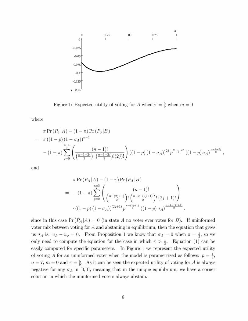
From Proposition 1 we know that when π ≥ 12a voter would never vote for B ifm = 0,
so σB = 0. Given this, the expected utility of an uninformed voter from voting for A,
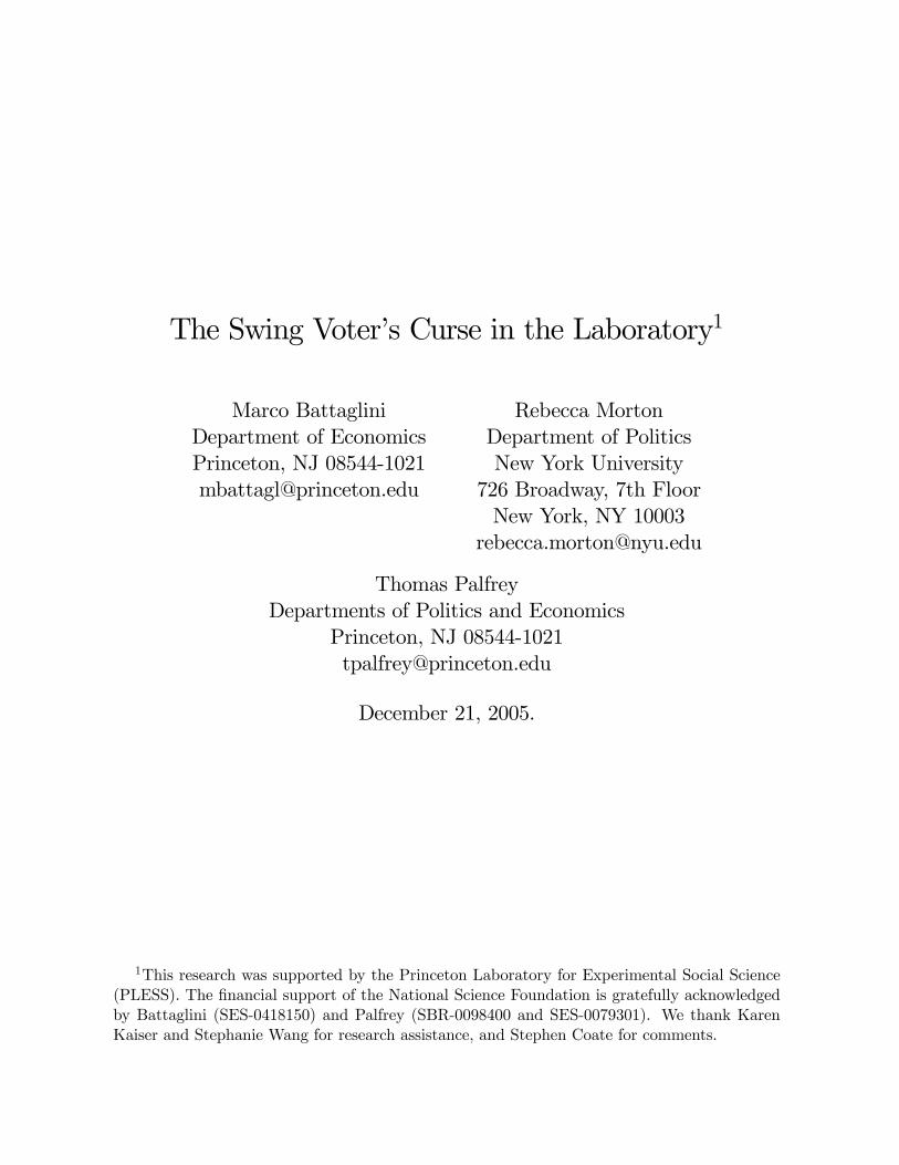
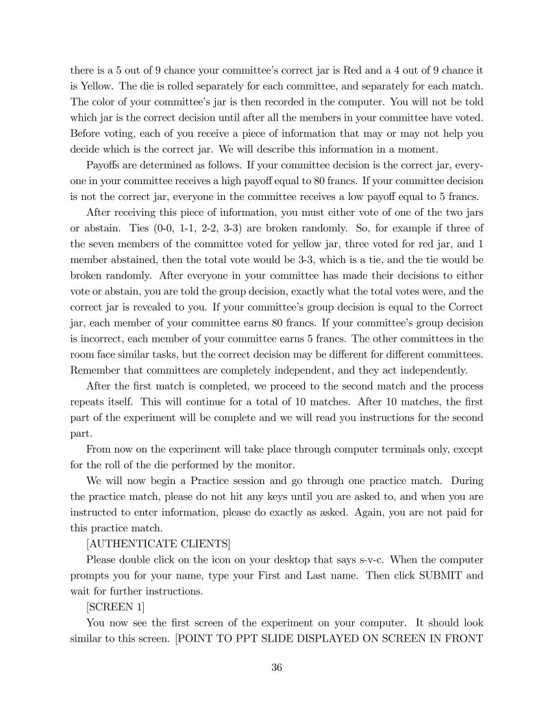
and therefore σA, can be easily computed. Let uA and uφ be respectively the expected
utilities of voting for A and abstaining for an uniformed voter, expressed as functions of
σA. The net utility of voting for A is:
uA − uφ =1
2[πPr (P0 |A)− (1− π) Pr (P0 |B )] (1)
+1
2[πPr (PA |A)− (1− π) Pr (PA |B )]
7
10.750.50.2500
-0.025
-0.05
-0.075
-0.1
-0.125
-0.15
x
y
x
y
Figure 1: Expected utility of voting for A when π = 59when m = 0
where
πPr (P0 |A)− (1− π) Pr (P0 |B )= π ((1− p) (1− σA))
n−1
− (1− π)
n−12X
j=0
Ã(n− 1)!¡
n−1−2j2
¢!¡n−1−2j
2
¢!(2j)!
!((1− p) (1− σA))
2j pn−1−2j
2 ((1− p)σA)n−1−2j
2 ,
and
πPr (PA |A)− (1− π) Pr (PA |B )
= − (1− π)
n−32X
j=0
⎛⎝ (n− 1)!³n−(2j+1)
2
´!³n−2−(2j+1)
2
´! (2j + 1)!
⎞⎠· ((1− p) (1− σA))
(2j+1) pn−(2j+1)
2 ((1− p) σA)n−2−(2j+1)
2 .
since in this case Pr (PA |A) = 0 (in state A no voter ever votes for B). If uninformed
voter mix between voting for A and abstaning in equilibrium, then the equation that gives
us σA is: uA − uφ = 0. From Proposition 1 we know that σA = 0 when π = 12, so we
only need to compute the equation for the case in which π > 12. Equation (1) can be
easily computed for specific parameters. In Figure 1 we represent the expected utility
of voting A for an uninformed voter when the model is parametrized as follows: p = 14,
n = 7, m = 0 and π = 59. As it can be seen the expected utility of voting for A is always
negative for any σA in [0, 1], meaning that in the unique equilibrium, we have a corner
solution in which the uninformed voters always abstain.
8

III.2 Partisan Bias
Let us now consider an environment in which A has a partisan advantage: m > 0 Assume
first that π = 12. In this case the swing voter’s curse is confounded by the bias introduced
by the partisans. Conditioning on the event in which the two alternatives receive the
same number of votes, the voter realizes that it is more likely that B has received some
votes from informative voters because he knows for sure that some of the votes cast in
favor of A, coming from partisans, are uninformative. Indeed, the voter may be willing to
vote for B, because doing so offsets a partisan vote. As in the previous case with m = 0,
the voters’ problem is more complicated when π > 12. In this case the prior probability
favors A, so the incentives to vote for B are weaker, and a voter will find it optimal to do
so only if there are enough informed voters in the population. This is summarized in the
following result:
Lemma 2 Let m > 0. If π = 12,then σA ≤ σB; if π > 1
2, then there is a p such that p > p
implies σA ≤ σB.
In this case too this result can be made more precise by showing that no voter would
ever vote for A:
Proposition 2 Letm > 0. If π = 12, or if π > 1
2and p is large enough, then σB > σA = 0.
III.3 Comparative Statics
The probability with which the uninformed voters vote for B depends on the paramethers
of the model, m, p, n, π. For example, the higher is the bias in favor of A, the higher is
the incentive for uninformed voters to offset it by voting for B. The exact probability σBcan be easily computed for specific parameter values when m > 0.10 From Proposition 1
we know that we only have one variable to determine, σB; and one equation to respect: in
a mixed strategy equilibrium the agent must be indifferent between abstaining and voting
for B. This indifference condition requires that the net expected utility of voting to be
zero. We can write the equilibrium condition as:
uB−uφ = 1
2[(1− π) Pr (P0 |B )− πPr (P0 |A)]+1
2[(1− π) Pr (PB |B )− πPr (PB |A)] = 0
10The case with m = 0 is not necessary since from Proposition 2 we know that the uninformed votersalways abstain.
9
10.750.50.250
0.2
0.15
0.1
0.05
0
-0.05
-0.1
-0.15
x
y
x
y
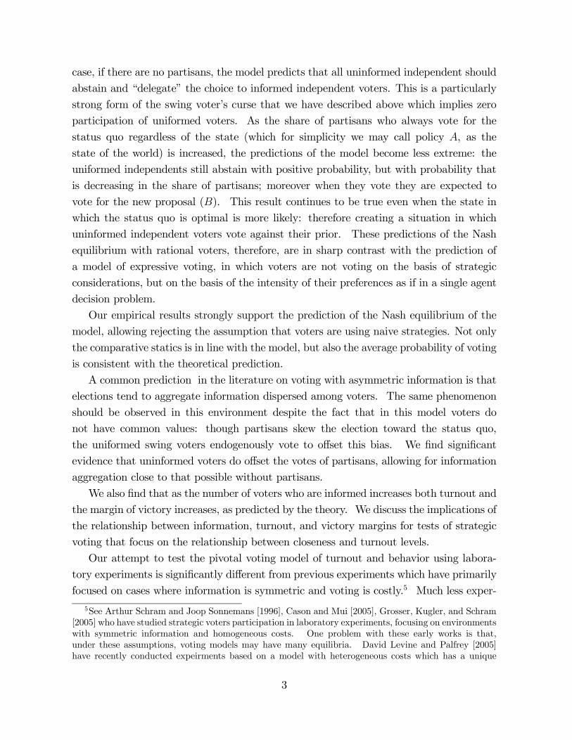
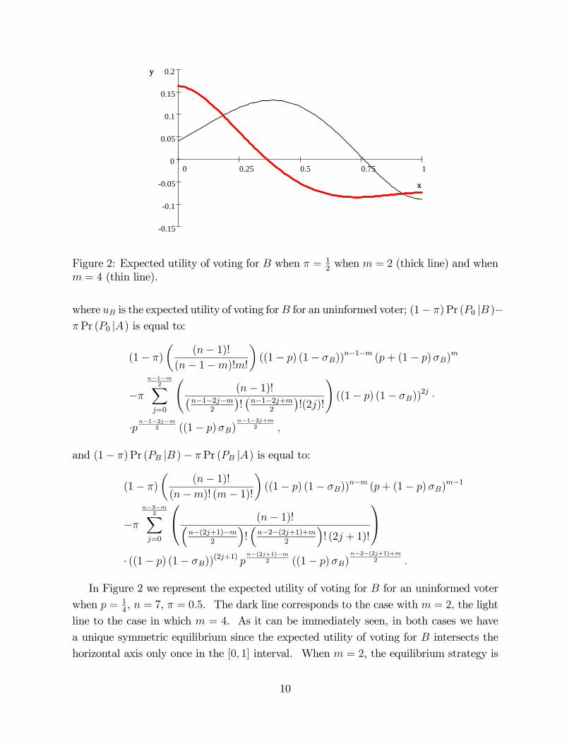
Figure 2: Expected utility of voting for B when π = 12when m = 2 (thick line) and when
m = 4 (thin line).
where uB is the expected utility of voting forB for an uninformed voter; (1− π) Pr (P0 |B )−πPr (P0 |A) is equal to:
(1− π)
µ(n− 1)!
(n− 1−m)!m!
¶((1− p) (1− σB))
n−1−m (p+ (1− p)σB)m
−πn−1−m
2Xj=0
Ã(n− 1)!¡
n−1−2j−m2
¢!¡n−1−2j+m
2
¢!(2j)!
!((1− p) (1− σB))
2j ·
·pn−1−2j−m2 ((1− p)σB)
n−1−2j+m2 ,
and (1− π) Pr (PB |B )− πPr (PB |A) is equal to:
(1− π)
µ(n− 1)!
(n−m)! (m− 1)!¶((1− p) (1− σB))
n−m (p+ (1− p)σB)m−1
−πn−3−m
2Xj=0
⎛⎝ (n− 1)!³n−(2j+1)−m
2
´!³n−2−(2j+1)+m
2
´! (2j + 1)!
⎞⎠· ((1− p) (1− σB))
(2j+1) pn−(2j+1)−m
2 ((1− p)σB)n−2−(2j+1)+m
2 .
In Figure 2 we represent the expected utility of voting for B for an uninformed voter
when p = 14, n = 7, π = 0.5. The dark line corresponds to the case with m = 2, the light
line to the case in which m = 4. As it can be immediately seen, in both cases we have
a unique symmetric equilibrium since the expected utility of voting for B intersects the
horizontal axis only once in the [0, 1] interval. When m = 2, the equilibrium strategy is
10
σB = 0.36; when m = 4, we have σB = 0.76.11
In a similar way we can find the equilibrium in the case in which π > 0.5. We have
explicitly computed the equilibrium when π = 59, and the other parameters are as above.
In this case too we have a unique equilibrium in correspondence of which with m = 2,
σB = 0.33, and with m = 4, σB = 0.73. Not surprisingly, a small increase in π has a
small effect on the equilibrium strategies and tends to reduce the probability of voting for
B.
Our results then provide testable predictions about voter behavior as a function of
π and m. Later we compare our results to alternative, decision-theoretic, models of
turnout as well. That is, if information increases turnout increases simply because voters
are more certain about their choices as posited by Matsusaka [1995], then we would
not expect uninformed voters to vote for B more often when there is a partisan bias as
compared to no bias. In voters vote on the basis of their prior, the change in π from .5
to .55 should induce them to vote for A, regardless of the partisan bias.12
IV Experimental Design
We use controlled laboratory experiments to evaluate the theoretical predictions. Once
a specific parametrization for n, m, and p is chosen, the model described and solved in
the previous section can be directly tested in the lab without changes. All the laboratory
experiments used n = 7 and p = 0.25. We used two different treatments for the state
of the world: π = 1/2 and π = 5/9 and three different treatments for partisan bias:
m = 0, 2, and 4. Table 1 summarizes the equilibrium strategies for each treatment as
derived in the previous section.
In the last row of Table 1 we contrast our theoretical predictions with those of the
decision theoretic approach of Matsusaka [1995]. Matsusaka assumes that voters partic-
ipate for consumption benefits that are independent of whether they are pivotal. These
consumption benefits are positively related to voters’ certainty over which choices yield
them the highest utility which depends on their information about the choices. When
voters’ are uninformed and perceived all options as equally likely, the decision-theoretic
model predicts that they will abstain, but that more precise information increases the
probability that they will vote.
Thus, in our experimental design, uninformed decision-theoretic voters should abstain
when π = 0.5, regardless of the size of the partisan bias. When π = 5/9, uninformed
11Unless otherwise noted in the paper, we round off to two decimal places.12This is also consistent with models of expressive voting. See, for example, Coate, Conlin, and Moro
[2004].
11

decision-theoretic voters should have a positive probability of voting for A and a zero
probability of voting for B, regardless of the size of the partisan bias.
Table 1: Equilibrium Strategies for Uninformed VotersProbability of State A
Partisan Bias π = 1/2 π = 5/9m = 0 σB = σA = 0 σA = σB = 0m = 2 σB = 0.36 > σA = 0 σB = 0.33 > σA = 0m = 4 σB = 0.76 > σA = 0 σB = 0.73 > σA = 0
Decision-Theoretic Voters σB = σA = 0 σA > σB = 0
The experiments were all conducted at the Princeton Laboratory for Experimental
Social Science and used registered students from Princeton University. Four sessions
were conducted, each with 14 subjects.13 Each subject participated in exactly one session.
Each session was divided into thirds, each of which lasted for 10 periods, with different
treatments in each subsession. Table 2 summarizes the experimental design.
Table 2: Experimental DesignPeriods in Subsessions
Session π 1-10 11-20 21-30 #Subjects1 1/2 m = 2 m = 4 m = 0 142 1/2 m = 4 m = 2 m = 0 143 5/9 m = 0 m = 4 m = 2 144 5/9 m = 0 m = 2 m = 4 14
Subjects were randomly divided into groups of seven for each period. Instructions
were read aloud and subjects were required to correctly answer all questions on a short
comprehension quiz before the experiment was conducted. Subjects were also provided
a summary sheet about the rules of the experiment which they could consult. The
experiments were conducted via computers.14 Subjects were told there were two possible
jars, Jar 1 and Jar 2. Jar 1 contained six white balls and two red; jar 2 contained six
white balls and two yellow. The monitor from the experiment randomly chose a jar for
each group in each period by tossing a fair die according to the value of π in the treatment
where jar 1 was equivalent to state A in the model and jar 2 was equivalent to state B in
the model.15 The balls were then shuffled in random order on each subject’s computer
screen, with the ball colors hidden. Each subject then privately selected one ball by
13Each session included one additional subject who was paid $20 to serve as a monitor.14The computer program used was similar to Battaglini, et al. [2005] as an extension to the open
source Multistage game software. See http://multistage.ssel.caltech.edu.15We used a 10 sided die with numbers 0-9 when π = 5/9, where numbers 1-5 resulted in state A,
numbers 6-9 resulted in state B, and if a number 0 was thrown, the die was thrown until 1-9 appeared.
12
clicking on it with the mouse revealing the color of the ball to that subject only. The
subject then chose whether to vote for jar 1, vote for jar 2, or abstain. In the treatments
without partisan bias, i.e. m = 0, if the majority of the votes cast by the group were for
the correct jar, each group member, regardless of whether he or she voted, received a payoff
of 80 cents. If the majority of the votes cast by the group were incorrect guesses, each
group member, regardless of whether he or she voted, received a payoff of 5 cents. Ties
were broken randomly. In the treatment with partisan bias, subjects were told that the
computer would cast m votes for jar 1 in each election. This was repeated for 30 periods,
with the variations described in Table 2 above, and with the group membership shuffled
randomly after each round. Each subject was paid the sum of his or her earnings over all
40 rounds in cash at the end of the experiment. Average earnings were approximately
$30 (including a $10 show up fee), with each session lasting about 60 minutes.
V Experimental Results
V.1 Aggregate Voter Choices
V.1.1 Informed Voters
Of the 1680 voting decisions we observed, in 422 cases (25.1%) subjects were informed,
that is, revealed a red or yellow ball. Across all treatments and sessions, these informed
voters chose 100% as predicted, 100% of the time if a voter revealed a red ball, he or she
voted for jar 1 (state A) and 100% of the time if a voter revealed a yellow ball, he or she
voted for jar 2 (state B). We interpret this as indicating that all subjects had a least a
basic comprehension of the task.
V.1.2 Uninformed Voters
Case 1: π = 0.5
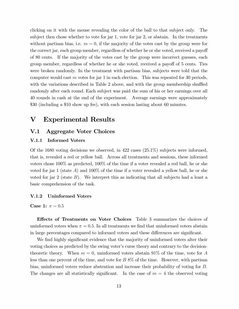
Effects of Treatments on Voter Choices Table 3 summarizes the choices of
uninformed voters when π = 0.5. In all treatments we find that uninformed voters abstain
in large percentages compared to informed voters and these differences are significant.
We find highly significant evidence that the majority of uninformed voters alter their
voting choices as predicted by the swing voter’s curse theory and contrary to the decision-
theoretic theory. When m = 0, uninformed voters abstain 91% of the time, vote for A
less than one percent of the time, and vote for B 8% of the time. However, with partisan
bias, uninformed voters reduce abstention and increase their probability of voting for B.
The changes are all statistically significant. In the case of m = 4 the observed voting
13
0.2
.4.6
.81
0 10 20 30 0 10 20 30
Session 1 Session 2
Pct Voting for A Pct Voting for BEquil. Prob. Vote A Equil. Prob. Vote B
Period
Graphs by Session With Pi = 0.5
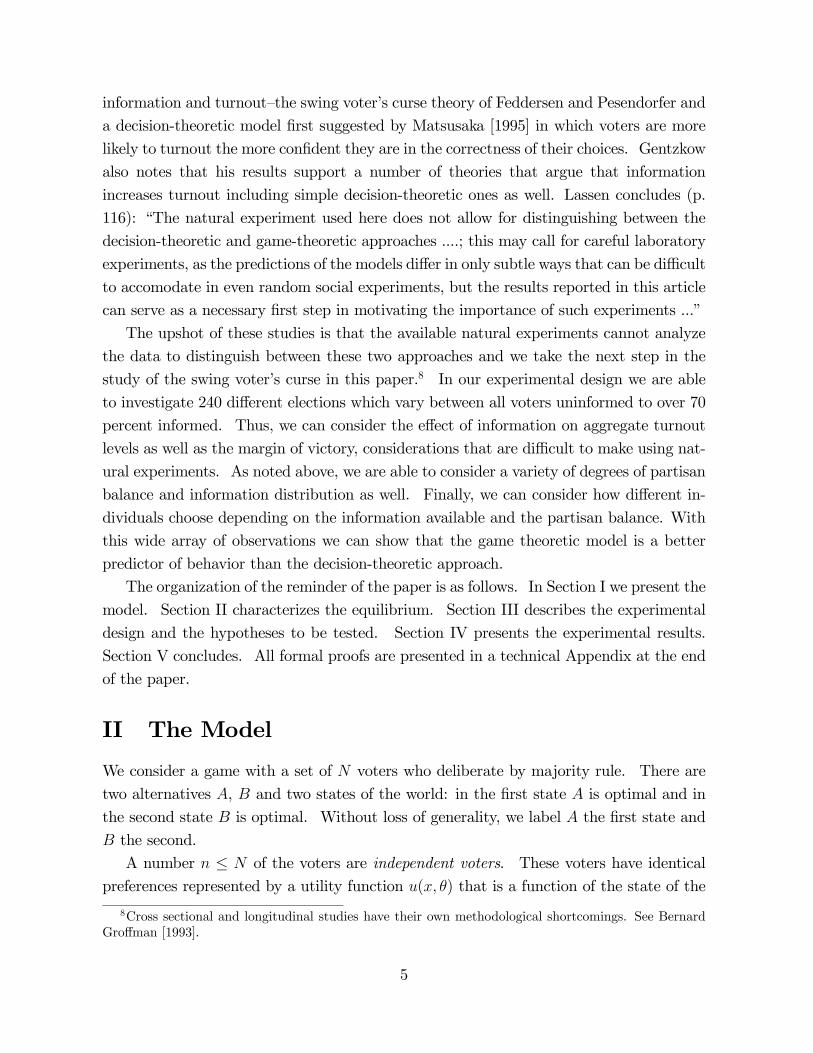
Uninformed Voter Decisions With Pi = 1/2
Figure 3:
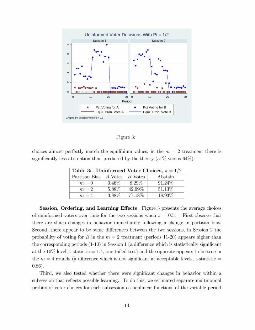
choices almost perfectly match the equilibium values; in the m = 2 treatment there is
significantly less abstention than predicted by the theory (51% versus 64%).
Table 3: Uninformed Voter Choices, π = 1/2Partisan Bias A Votes B Votes Abstain
m = 0 0.46% 8.29% 91.24%m = 2 5.88% 42.99% 51.13%m = 4 3.88% 77.18% 18.93%
Session, Ordering, and Learning Effects Figure 3 presents the average choices
of uninformed voters over time for the two sessions when π = 0.5. First observe that
there are sharp changes in behavior immediately following a change in partisan bias.
Second, there appear to be some differences between the two sessions, in Session 2 the
probability of voting for B in the m = 2 treatment (periods 11-20) appears higher than
the corresponding periods (1-10) in Session 1 (a difference which is statistically significant
at the 10% level, t-statistic = 1.4, one-tailed test) and the opposite appears to be true in
the m = 4 rounds (a difference which is not significant at acceptable levels, t-statistic =
0.86).
Third, we also tested whether there were significant changes in behavior within a
subsession that reflects possible learning. To do this, we estimated separate multinomial
probits of voter choices for each subsession as nonlinear functions of the variable period
14

0.2
.4.6
.81
0 10 20 30 0 10 20 30
Session 1 Session 2
Multinomial Probit Est. Prob. Vote A Multinomial Probit Est. Prob. Vote BEquil. Prob. Vote A Equil. Prob. Vote B
Period
Graphs by Session With Pi = 0.5
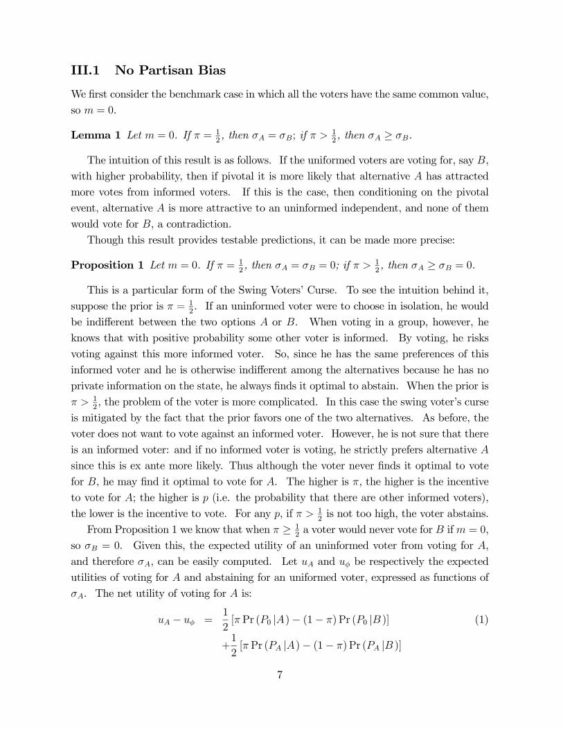
Estimated Learning With Pi = 1/2
Figure 4:
in the subsession (results from these estimations are presented in Appendix, note that
the standard errors in the estimations were adjusted for clustering by subject).16 The
estimated probabilities by period are presented in Figure 4 below. As can be seen from
the figure, subjects’ voting behavior appears to demonstrate learning in early periods in
all the subsessions (with some slight increase in nonrational choices towards the end of
a subsession) except for the case where m = 2 when subjects not only vote more for B
than the equilibrium level, but increase their voting for B during the early periods in the
subsessions with some evidence of learning in later periods in the subsession.
Case 2: π = 5/9
Effects of Treatments on Voter Choices Table 4 summarizes uninformed voter
choises when the probability of state A = 5/9. Again, we find that in all treatments unin-
formed voters abstain large percentages compared to informed voters and these differences
16Multinomial probit or logit is appropriate since the dependent variable is an unordered multinomialresponse, multinomial logit yielded the same qualitative results. The model was fitted via maximumlikelihood in Stata 9. As an alternative to clustering observations by subject, we estimated a fixed effectsversion of multinomial logit (multinomial probit failed to converge in most subsessions) with largely thesame qualitative predictions although in some cases the data was insufficient for accurate predictions.See Jeffrey M. Woolbridge [2002], pages 496-504 for a discussion of multinomial response models andcluster sampling procedures for their estimation.
15
are significant, as predicted by the swing voter’s curse theory.
We find some support, however, for the decision-theoretic model of voting whenm = 0
as voting for A is significantly higher than when π = 0.5 (19.7% compared to 0.46%). But
the decision-theoretic model falters as partisan bias increases and we again find highly
significant evidence that uninformed voters alter their voting choices as predicted by the
swing voter’s curse theory and contrary to the decision-theoretic theory. With partisan
bias, voting for A when π = 5/9 is not significantly different from voting for A when
π = 0.5, as predicted by the swing voter’s curse theory and contrary to the decision-
theoretic approach. With partisan bias, the percent of uninformed voters voting for B
increases with m, from 7% to 30% to 58% for m = 0, 2, 4, respectively. All of these
differences are highly significant.
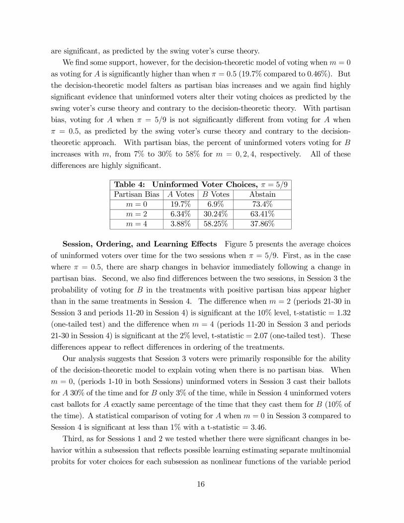
Table 4: Uninformed Voter Choices, π = 5/9Partisan Bias A Votes B Votes Abstain
m = 0 19.7% 6.9% 73.4%m = 2 6.34% 30.24% 63.41%m = 4 3.88% 58.25% 37.86%
Session, Ordering, and Learning Effects Figure 5 presents the average choices
of uninformed voters over time for the two sessions when π = 5/9. First, as in the case
where π = 0.5, there are sharp changes in behavior immediately following a change in
partisan bias. Second, we also find differences between the two sessions, in Session 3 the
probability of voting for B in the treatments with positive partisan bias appear higher
than in the same treatments in Session 4. The difference when m = 2 (periods 21-30 in
Session 3 and periods 11-20 in Session 4) is significant at the 10% level, t-statistic = 1.32
(one-tailed test) and the difference when m = 4 (periods 11-20 in Session 3 and periods
21-30 in Session 4) is significant at the 2% level, t-statistic = 2.07 (one-tailed test). These
differences appear to reflect differences in ordering of the treatments.
Our analysis suggests that Session 3 voters were primarily responsible for the ability
of the decision-theoretic model to explain voting when there is no partisan bias. When
m = 0, (periods 1-10 in both Sessions) uninformed voters in Session 3 cast their ballots
for A 30% of the time and for B only 3% of the time, while in Session 4 uninformed voters
cast ballots for A exactly same percentage of the time that they cast them for B (10% of
the time). A statistical comparison of voting for A when m = 0 in Session 3 compared to
Session 4 is significant at less than 1% with a t-statistic = 3.46.
Third, as for Sessions 1 and 2 we tested whether there were significant changes in be-
havior within a subsession that reflects possible learning estimating separate multinomial
probits for voter choices for each subsession as nonlinear functions of the variable period
16
0.2
.4.6
.81
0 10 20 30 0 10 20 30
Session 3 Session 4
Pct Voting for A Pct Voting for BEquil. Prob. Vote A Equil. Prob. Vote B
Period
Graphs by Session With Pi = 5/9
Uninformed Voter Decisions With Pi = 5/9
Figure 5:
in the subsession as above (see Appendix for detailed results). The estimated probabil-
ities by period are presented in Figure 6 below. As in the analysis above, we find that
learning tends to occur early in subsessions. We find evidence that voter learning trends
towards the swing voter’s curse theory as compared to the decision-theoretic model; un-
informed voters decrease their probability of voting for A as the number of periods in a
subsession increases, even in the one case where the decision-theoretic model outperforms
the swing-voter’s curse (Session 3 when m = 0).
V.2 Committee Decisions
V.2.1 Information and Turnout
In the previous subsection we averaged across all committees within a treatment. We now
turn to an analysis of committee decisions. First we examine therelationship between
turnout and the number of informed voters. Theoretically, we expect that as the number
of informed voters increases, the turnout level will increase from σB to 1. That is, in
equilibrium informed voters vote 100% of the time, while uninformed voters cast votes
with probability σB. When a voter becomes informed then total turnout increases by 1
and decreases by only σB.
To evaluate this prediction we estimate the effect of increasing the number of informed
voters in a group on the number of voters in the group who chose to vote (including both
17

0.2
.4.6
.81
0 10 20 30 0 10 20 30
Session 3 Session 4
Multinomial Probit Est. Prob. Vote A Multinomial Probit Est. Prob. Vote BEquil. Prob. Vote A Equil. Prob. Vote B
Period
Graphs by Session With Pi = 5/9
Estimated Learning With Pi = 5/9
Figure 6:
informed and uninformed voters but excluding of course computer voters). We take
our individual voter predictions from the multinomial probit estimations described above
and summarized in the Appendix for each voter in each committee in each period in each
session to construct a mean committee turnout level by number of informed voters for each
subsession. This allows us to estimate the relationship between the number of informed
voters and committee turnout levels incorporating individual subject and learning effects
that might affect committee turnout levels.17
Figure 7 presents a comparison of the estimated turnout levels with the actual mean
turnout levels of the committees and the swing voter’s curse theoretically predicted
turnout levels as a function of the number of informed voters. These relationships are
only shown for the range of informed voters realized in the subsession—in some subsessions
there were no committees with more than 3 informed voters. First notice that although
the estimated relationships are nonlinear, reflecting the effects of learning and subject co-
horts, the estimated relationships’ slopes closely track the theoretical slopes. Thus, even
with such effects, our comparative static prediction of the relationship between number
17We also estimated separate binomial regressions, as described in Wooldridge [2002] pages 659-660,to estimate votes for A and for B, which we then used to construct estimated turnout levels by numberof informed voters for each subsession. These levels were similar to the ones reported here, but assumean independence between the votes for A and B. We also estimated a binomial regression where thedependent variable was aggregate turnout with similar results. Using the multinomial probit estimationsallow us to consider subject specific effects and learning that might affect committee turnout choices.
18

02
46
80
24
68
0 1 2 3 4 5 0 1 2 3 4 5 0 1 2 3 4 5
Pi = 1/2, m = 0 Pi = 1/2, m = 2 Pi = 1/2, m = 4
Pi = 5/9, m = 0 Pi = 5/9, m = 2 Pi = 5/9, m = 4
Equilibrium Turnout Mean TurnoutEstimated Turnout
Turn
out o
f Non
-Par
tisan
Vot
ers
Number of Informed Voters
Graphs by Probability of State A and Partisan Bias
Committee Turnout Levels Excluding Partisan Votes
Figure 7:
of informed voters and committee turnout receives support. Furthermore, as partisan
bias increases, the relationship between turnout and number of informed voters becomes
flatter as expected.
Second, except for the case when m = 4 and π = 5/9, estimated actual turnout
exceeds equilibrium turnout, reflecting the tendency of uninformed voters to vote more
than predicted when there is zero partisan bias or low levels of partisan bias. When
m = 4 and π = 0.5 the estimated turnout relationships almost perfectly coincide with
the equilibrium relationship. These results are consistent with the aggregate individual
behavior results reported above; when partisan bias is low, uninformed voters tend to
vote more than predicted, but when partisan bias is high, uninformed voters vote either
less or very close to the equilibrium predicted levels.
V.2.2 Margin of Victory and Information
As the number of informed voters in a committee is expected to affect turnout, it is also
expected to affect the margin of victory for the winning outcome. We also evaluate
this comparative static prediction by comparing estimated committee margins of victory
calculated using the estimated individual probabilities of voting by subject, period, and
subsession with the equilibrium probabilties. However, the theoretically predicted margin
of victory depends on the signals received by informed voters and thus the true state.
For example, if the true state is A and the number of informed voters are 4, m = 4, and
19

-20
24
68
-20
24
68
0 1 2 3 4 5 0 1 2 3 4 5 0 1 2 3 4 5
Pi = 1/2, m = 0 Pi = 1/2, m = 2 Pi = 1/2, m = 4
Pi = 5/9, m = 0 Pi = 5/9, m = 2 Pi = 5/9, m = 4
Equilbrium EstimatedMean Tied Election
Plur
ality
for A
Number of Informed Voters
Graphs by Probability of State A and Partisan Bias
Plurality for A When A is True State Including Partisans
Figure 8:
π = 0.5, theoretically we expect a victory margin of |8− 3(0.78)| = 5. 66 while if the truestate is B theoretically we expect a victory margin of |4− 3(0.78)− 4| = 2. 34. Thus wemake two comparisons, we compare the estimated plurality for A with the equilibrium
plurality for A when the true state is A and we compare the estimated plurality for B
with the equilibrium plurality for B when the true state is B. Figures 8 and 9 present
these comparisons.
In the figures, the light solid line represents when an election was tied. Observations
below this line represent wins by state B and above the line represent wins by state A
in Figure 8 and vice-versa in Figure 9. Thus, observations below this line represent cases
where committees chose incorrectly, while observations above this line represent cases
where committees chose correctly.
First notice that as with the turnout levels, the slope of the equilibrium plurality re-
lationships depend on the degree of partisan bias and the estimated relationships demon-
strate similar dependence. Second, we find that generally the margins of victory for A
are greater than equilibrium when A is the true state and the margins of victory for B are
less than equilibrium when B is the true state, which follows from the excess voting for A.
Third we find that it takes very few informed voters for the true state to have a positive
margin of victory—in most cases with just one informed voter, the plurality of votes in
favor of the true state is positive, even when m = 4. Thus, uninformed voters sufficiently
balance out the partisan bias such that the true state receives a positive plurality.
20

-20
24
-20
24
0 1 2 3 4 5 0 1 2 3 4 5 0 1 2 3 4 5
Pi = 1/2, m = 0 Pi = 1/2, m = 2 Pi = 1/2, m = 4
Pi = 5/9, m = 0 Pi = 5/9, m = 2 Pi = 5/9, m = 4
Equilbrium EstimatedMean Tied Election
Plur
ality
for B
Number of Informed Voters
Graphs by Probability of State A and Partisan Bias
Plurality for B When B is True State Including Partisans
Figure 9:
V.2.3 Closeness and Turnout
A common perceived prediction of the rational model of voting is that turnout should be
positively related to the expected closeness of an election since when elections are expected
to be close, votes are more likely to be pivotal, and thus the investment benefits from
voting are greater.18 However, in our analysis closeness and turnout may be negatively
related since increasing the number of informed voters increases the margin of victory
(decreasing closeness) while it increases turnout. These results imply that simple tests of
the effect of closeness on turnout decisions or aggregate turnout are not nuanced enough
to determine if voters are making participation decisions rationally.
V.2.4 Efficiency of Committee Choices
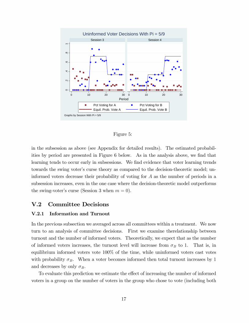
Figure 10 below shows the percentage of correct committee choices as a function of the
number of informed voters when π = 0.5 (Note that we omit cases where we have no ob-
servations, for example, we have no observations whenm < 4 and the number of informed
voters is greater than 3). We compare these percentages to the percentages theoretically
predicted to be correct which are calculated by estimating the binomial probabilities that
a group is correct given the assumed number of informed voters. We find that group
decisions are generally either more likely to be correct than theoretically predicted or close
18See for example Filer, Kenny, and Morton [1993].
21
Actual Versus Predicted Percent Correct, Probability of State A = 1/2
0%
10%
20%
30%
40%
50%
60%
70%
80%
90%
100%
0 (21 obs.) 1 (39 obs.) 2 (30 obs.) 3 or greater (30 obs.)
Number of Informed Voters
Perc
ent C
orre
ct
Actual, m = 0 Predicted, m=0 Actual, m = 2 Predicted, m = 2 Actual, m = 4 Predicted, m = 4
Figure 10:
to the theoretical prediction. The largest and only statistically significant shortfall occurs
when only one voter is informed and m = 0, theory predicts that the group decision will
be correct 100% of the time, we find that the group decisions are correct only 87.5% of the
time, which is significant at a 2% confidence level. In some cases, due to fortunate draws,
the group decisions are correct a greater percentage of time than theoretically predicted.
For example, when m = 0 and no voter is informed, we predict that the group will be
correct 50% of the time, we find in the experiment that the group is correct 62.5% of the
time. None of these differences are statistically significant, however.
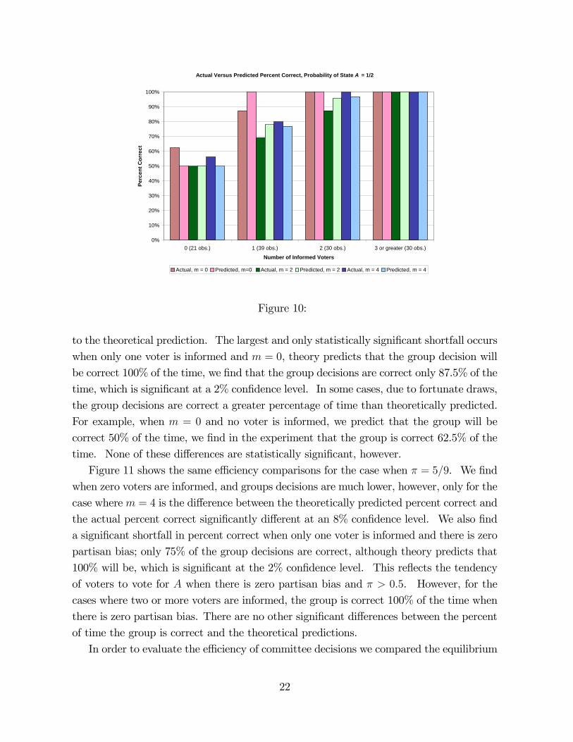
Figure 11 shows the same efficiency comparisons for the case when π = 5/9. We find
when zero voters are informed, and groups decisions are much lower, however, only for the
case wherem = 4 is the difference between the theoretically predicted percent correct and
the actual percent correct significantly different at an 8% confidence level. We also find
a significant shortfall in percent correct when only one voter is informed and there is zero
partisan bias; only 75% of the group decisions are correct, although theory predicts that
100% will be, which is significant at the 2% confidence level. This reflects the tendency
of voters to vote for A when there is zero partisan bias and π > 0.5. However, for the
cases where two or more voters are informed, the group is correct 100% of the time when
there is zero partisan bias. There are no other significant differences between the percent
of time the group is correct and the theoretical predictions.
In order to evaluate the efficiency of committee decisions we compared the equilibrium
22

Actual Versus Predicted Correct, Probability of State A = 5/9
0%
10%
20%
30%
40%
50%
60%
70%
80%
90%
100%
0 (16 obs.) 1 (33 obs.) 2 (35 obs.) 3 or greater (36 obs.)
Number of Informed Voters
Pere
cent
Cor
rect
Actual, m = 0 Predicted, m=0 Actual, m = 2 Predicted, m = 2 Actual, m = 4 Predicted, m = 4
Figure 11:
probabilities that a committee will make a correct decision for each treatment with the
estimated probabilities calculated using the probabilities of voting for A, B, or abstaining
as estimated by period, group, and treatment in the multinomial probits discussed above.
This is shown in figures 12-13.
We control for the true state and the number of informed voters since informed voters
voted their signals 100% of the time. For example, consider a committee where m = 0,
A is the true state, π = 0.5, and there are seven uninformed voters. In this case, we
only need to compute the probability that the number of votes received by A is greater
than the number of votes received by B. We do so by calculating the probability of
this event given the estimated individual probabilities of voting for A,B, or abstaining
from the multinomial probits for this committee which depended on the session and the
period of the experiment. Similarly, in a committee where m = 4, B is the true state,
π = 0.5, and there are five uninformed voters, we need to compute the probability that
the number of uninformed voters for B exceeds the number of uninformed voters for A
by more than 2 (since A will get 4 computer votes and the 2 informed voters will vote for
B). We performed these calculations for each committee and the particular configuration
of computer votes, true state, and number of informed voters.
We find that the committees tend to be less efficient in decision making when π = 5/9
and/or the true state is B. However, the committee decisions, like the equilibrium deci-
sions, are approximately 100% correct if there are 3 or more informed voters, even when
23

0.2
.4.6
.81
0.2
.4.6
.81
0 1 2 3 0 1 2 3 0 1 2 3
Pi = 1/2, m = 0 Pi = 1/2, m = 2 Pi = 1/2, m = 4
Pi = 5/9, m = 0 Pi = 5/9, m = 2 Pi = 5/9, m = 4
Equilbrium Estimated
Pro
babi
lity
Com
mitt
ee's
Dec
isio
n is
Cor
rect
Number of Informed Voters
Graphs by Probability of State A and Partisan Bias
Efficiency of Committee Decisions When A is True State
Figure 12:
0.2
.4.6
.81
0.2
.4.6
.81
0 1 2 3 0 1 2 3 0 1 2 3
Pi = 1/2, m = 0 Pi = 1/2, m = 2 Pi = 1/2, m = 4
Pi = 5/9, m = 0 Pi = 5/9, m = 2 Pi = 5/9, m = 4
Equilbrium Estimated
Prob
abilit
y C
omm
ittee
's D
ecis
ion
is C
orre
ct
Number of Informed Voters
Graphs by Probability of State A and Partisan Bias
Efficiency of Committee Decisions When B is True State
Figure 13:
24
there are four computer voters and the true state is B. Thus, balancing by uninformed
voters does help the committees reach more informed decisions than would be reached if
uninformed voters voted naively as predicted by the decision-theoretic model.
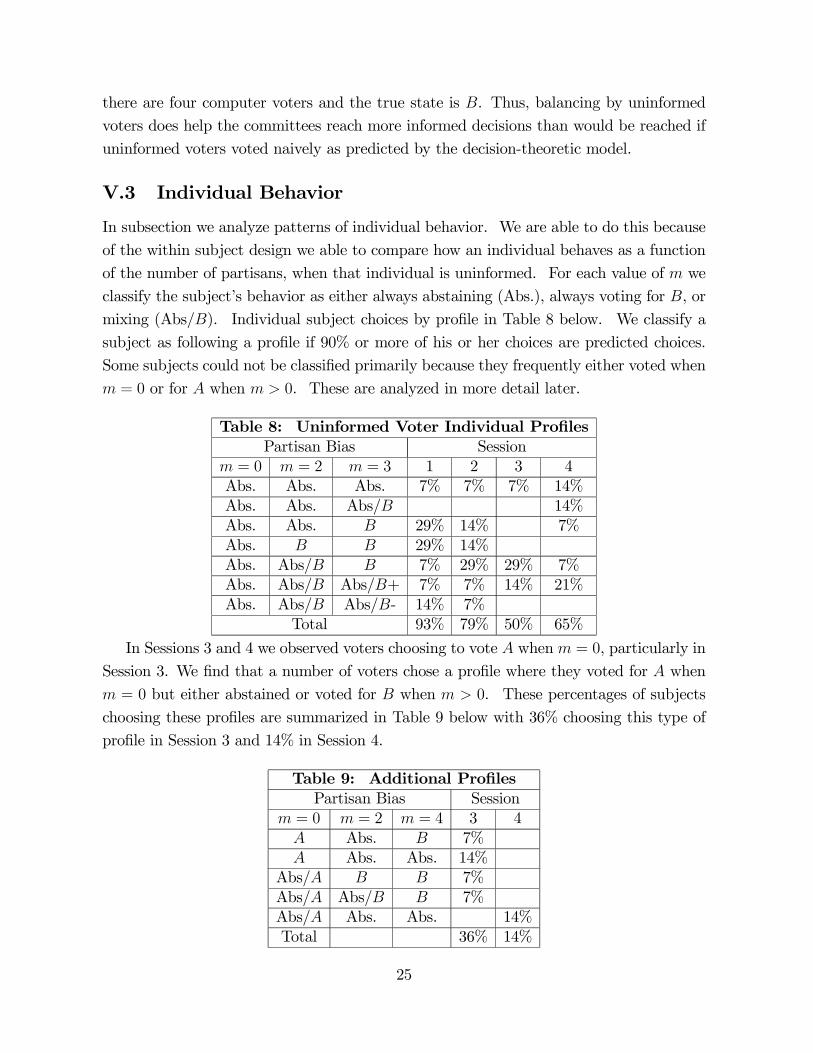
V.3 Individual Behavior
In subsection we analyze patterns of individual behavior. We are able to do this because
of the within subject design we able to compare how an individual behaves as a function
of the number of partisans, when that individual is uninformed. For each value of m we
classify the subject’s behavior as either always abstaining (Abs.), always voting for B, or
mixing (Abs/B). Individual subject choices by profile in Table 8 below. We classify a
subject as following a profile if 90% or more of his or her choices are predicted choices.
Some subjects could not be classified primarily because they frequently either voted when
m = 0 or for A when m > 0. These are analyzed in more detail later.
Table 8: Uninformed Voter Individual ProfilesPartisan Bias Session
m = 0 m = 2 m = 3 1 2 3 4Abs. Abs. Abs. 7% 7% 7% 14%Abs. Abs. Abs/B 14%Abs. Abs. B 29% 14% 7%Abs. B B 29% 14%Abs. Abs/B B 7% 29% 29% 7%Abs. Abs/B Abs/B+ 7% 7% 14% 21%Abs. Abs/B Abs/B- 14% 7%
Total 93% 79% 50% 65%
In Sessions 3 and 4 we observed voters choosing to vote A when m = 0, particularly in
Session 3. We find that a number of voters chose a profile where they voted for A when
m = 0 but either abstained or voted for B when m > 0. These percentages of subjects
choosing these profiles are summarized in Table 9 below with 36% choosing this type of
profile in Session 3 and 14% in Session 4.
Table 9: Additional ProfilesPartisan Bias Session
m = 0 m = 2 m = 4 3 4A Abs. B 7%A Abs. Abs. 14%
Abs/A B B 7%Abs/A Abs/B B 7%Abs/A Abs. Abs. 14%Total 36% 14%
25

VI Concluding Remarks
Significant evidence exists that voters often choose to abstain when voting is apparently
costless and the standard rational model of voting would predict participation. Empirical
analysis suggests that such abstention may be related to differences in voter information.
The Swing Voter’s Curse theory provides a complicated game theoretic explanation for
why uninformed voters would be willing to abstain and delegate decision making to more
informed voters. Hence, it is a candidate explanation for the empirical evidence that
lower information elections have lower turnout. In this paper we have provided the first
experimental test of the theory, where we control for key parameters of the model, which
are difficult to measure precisely or control for in naturally occuring data. We find
strong support for the theory. Uninformed voters behave strategically: they strategically
abstain when uninformed and both outcomes are equally likely, delegating their votes
to more informed voters. With partisan bias, they vote strategically to balance out the
votes of partisans, at probabilities close to equilibrium, increasing the probability of voting
as partisan bias increases. Even when the partisan-favored outcome is the more likely
outcome we find most voters balancing in this way. These results are supported at both
the aggregate and individual level and across sessions and treatment configurations.
We also find that turnout and margin of victory both increase with the number of
informed voters and that there is a positive relationship between these two variables,
contrary to the common view that rational models of turnout predict that closeness and
turnout should be positively related. These results suggest that tests using field data
of whether turnout is related to closeness, which are unable to control for information
asymmetries, are inadequate or at best very weak tests of rational voting models.
26

VII Appendix
VII.1 Proof of Lemma 1
Let uθ for θ = A,B be the expected utility of an uninformed swing voter of voting for
policy θ. To evaluate uA − uB there are only three relevant events: P0, the event when
there is a tie among the other voters between A and B; and Pθ for θ = A,B, which is the
event in which policy θ is losing by one vote. The expected net utility of voting for A
rather than B conditional on event Pi is
E (uA − uB |Pi ) =
½Pr(A |Pi )− 0.5 i = A,B2Pr(A |Pi )− 1 i = 0
We can therefore write:
uA − uB = [πPr (P0 |A)− (1− π) Pr (P0 |B )] + 12
Xi=A,B
Pr(Pi) (2Pr(A |Pi )− 1) (2)
= [πPr (P0 |A)− (1− π) Pr (P0 |B )] + 12
∙πPr (PB |A)− (1− π) Pr (PB |B )+πPr (PA |A)− (1− π) Pr (PA |B )
¸(3)
=
µΛ0 +
1
2Λ1
¶(4)
where Λ0 = [πPr (P0 |A)− (1− π) Pr (P0 |B )] and
Λ1 = πPr (PB |A)− (1− π) Pr (PB |B ) + πPr (PA |A)− (1− π) Pr (PA |B )
Consider Λ1 first. Since n is odd, we can write:
Λ1 =
n−32X
j=0
⎛⎝ (n− 1)!³n−(2j+1)
2
´!³n−2−(2j+1)
2
´! (2j + 1)!
⎞⎠ [(1− p)σφ](2j+1)
· [p+ (1− p) (1− σφ)] ·
⎧⎪⎪⎪⎪⎨⎪⎪⎪⎪⎩π
∙p (1− p)σB
+(1− p)2 σAσB
¸n−(2j+1)−22
− (1− π)
∙p (1− p)σA
+(1− p)2 σAσB
¸n−(2j+1)−22
⎫⎪⎪⎪⎪⎬⎪⎪⎪⎪⎭Consider now Λ0. We can write:
Λ0 =
n−12X
j=0
Ã(n− 1)!¡
n−1−2j2
¢!¡n−1−2j
2
¢! (2j)!
![(1− p)σφ]
2j
·(
π£p (1− p)σB + (1− p)2 σAσB
¤n−1−2j2
− (1− π)£p (1− p)σA + (1− p)2 σAσB
¤n−1−2j2
)> 0
27
Assume by contradiction that σB > σA. Since π ≥ 12, we conclude that Λ1 > 0 and
Λ0 > 0. So uA − uB > 0, which implies that σB ≤ σA, a contradiction. We conclude
that σA ≥ σB. When π = 12we can make the symmetric argument and prove σB ≥ σA.
Hence π = 12⇒ σB = σA. ¥
VII.2 Proof of Proposition 1
If σB > 0, then the voter must be indifferent between the two alternatives since σA ≥ σB
∀π ≥ 12. Assume this is the case, then:
0 = uA − uB = Pr [P0] · [2 Pr(A |P0 )− 1]+1
2Pr [PA] · [2 Pr(A |PA )− 1] v + 1
2Pr [PB] · [2 Pr(A |PB )− 1]
This equation implies:
[πPr (P0 |A)− (1− π) Pr (P0 |B )] (5)
=1
2[(1− π) Pr (PB |B )− πPr (PB |A)] + 1
2[(1− π) Pr (PA |B ) + πPr (PA |A)]
Moreover, we have:
uA − uφ =1
2[πPr (P0 |A)− (1− π) Pr (P0 |B )] + 1
2[πPr (PA |A)− (1− π) Pr (PA |B )]
(6)
Substituting (5) in (6), we obtain:
uA − uφ =1
4π [Pr (PA |A)− Pr (PB |A)] + 1
4(1− π) [Pr (PB |B )− Pr (PA |B )]
We can compute:
Pr (PB |B ) =n−32X
j=0
Φ(j)
£p(1− p)σA + (1− p)2 σAσB
¤p+ (1− p)σB
n−(2j+1)2
Pr (PB |A) =n−32X
j=0
Φ(j)
£p(1− p)σB + (1− p)2 σAσB
¤(1− p)σB
n−(2j+1)2
and
Pr (PA |A) =n−32X
j=0
Φ(j)
£p(1− p)σB + (1− p)2 σAσB
¤p+ (1− p)σA
n−(2j+1)2
Pr (PA |B ) =n−32X
j=0
Φ(j)
£p(1− p)σA + (1− p)2 σAσB
¤(1− p)σA
n−(2j+1)2
28

where: Φ(j) =
µ(n−1)!
(n−(2j+1)2 )!(n−2−(2j+1)2 )!(2j+1)!
¶[(1− p)σφ]
(2j+1). From these expressions
is evident that [Pr (PA |A)− Pr (PB |A)] < 0 and [Pr (PB |B )− Pr (PA |B )] < 0, which
implies that uA−uφ < 0, and therefore σA = 0. So σB ≤ σA = 0, a contradiction. Using
Lemma 1, we conclude that π = 12implies σA = σB = 0; and π > 1
2implies σA ≥ σB = 0,
as stated in the proposition. ¥
VII.3 Proof of Lemma 2
Assume by contradiction that m > 0 and σA ≥ σB. The expected utility of voting for A
net of the utility of voting for B can be expressed as in (2) and 3. In this case:
Λ1 =
n−3−m2X
j=0
⎛⎝ (n− 1)!³n−(2j+1)−m
2
´!³n−2−(2j+1)+m
2
´! (2j + 1)!
⎞⎠ [(1− p)σφ](2j+1)
· [p+ (1− p) (1− σφ)]
·
⎧⎪⎨⎪⎩ πh
(1−p)σBp+(1−p)σA
im2 £
p (1− p)σB + (1− p)2 σAσB¤n−(2j+1)−2
2
− (1− π)hp+(1−p)σB(1−p)σA
im2 £
p (1− p)σA + (1− p)2 σAσB¤n−(2j+1)−2
2
⎫⎪⎬⎪⎭Consider now Λ0. We can write:
Λ0 =
n−1−m2X
j=0
Ã(n− 1)!¡
n−1−2j−m2
¢!¡n−1−2j+m
2
¢(2j)!
![(1− p)σφ]
2j
·
⎧⎪⎨⎪⎩ πh
(1−p)σBp+(1−p)σA
im2 £
p (1− p)σB + (1− p)2 σAσB¤n−2j−1
2
− (1− π)hp+(1−p)σB(1−p)σA
im2 £
p (1− p)σA + (1− p)2 σAσB¤n−2j−1
2
⎫⎪⎬⎪⎭ < 0
Consider first the case in which π = 12, and assume by contradiction that σA > σB.
Since (1−p)σ(B)p+(1−p)σ(A) <
p+(1−p)σ(B)(1−p)σ(A) we have Λ0 < 0 and Λ1 < 0: so < 0, which implies that
σB ≥ σA, a contradiction. Consider now the case in which π > 12. There is a p such
that πh
(1−p)σBp+(1−p)σA
im2< (1− π)
hp+(1−p)σB(1−p)σA
im2for any p > p. Assume by contradiction that
σA > σB and p ≥ p. In this case too Λ0 < 0 and Λ1 < 0: so again uA − uφ < 0, which
implies that σB ≥ σA, a contradiction. ¥
VII.4 Proof of Proposition 2
Assume that σA > 0, then since σB ≥ σA, it must be that uA − uB = 0. Proceeding as
in Proposition 1 we can obtain:
uA − uφ =1
4π [Pr (PA |A)− Pr (PB |A)] + 1
4(1− π) [Pr (PB |B )− Pr (PA |B )]
29

We can compute:
Pr (PB |B ) =n−32X
j=0
Φ(j)
£p(1− p)σA + (1− p)2 σAσB
¤p+ (1− p)σB
n−(2j+1)−m2
Pr (PB |A) =n−32X
j=0
Φ(j)
£p(1− p)σB + (1− p)2 σAσB
¤(1− p)σB
n−(2j+1)−m2
and
Pr (PA |A) =n−32X
j=0
Φ(j)
£p(1− p)σB + (1− p)2 σAσB
¤p+ (1− p)σA
n−(2j+1)−m2
Pr (PA |B ) =n−32X
j=0
Φ(j)
£p(1− p)σA + (1− p)2 σAσB
¤(1− p)σA
n−(2j+1)−m2
where: Φ(j) =µ
(n−1)!(n−(2j+1)−m2 )!(n−2−(2j+1)+m2 )!(2j+1)!
¶((1− p) (1− σ))(2j+1). From these ex-
pressions is evident that [Pr (PA |A)− Pr (PB |A)] < 0 and [Pr (PA |B )− Pr (PB |B )] < 0,which implies that uA − uφ < 0: and therefore σA = 0, a contradiction.
We now prove that σB > 0. If this is not the case, the only other possibility is that
σB = σA = 0: we now show that this is impossible. We can write:
uB − uφ =1
2(1− π) Pr (P0 |B )− πPr (P0 |A) + 1
2[(1− π) Pr (PB |B )− πPr (PB |A)]
Since when σB = σA = 0 we have Pr (P0 |A) = Pr (PB |A) = 0, and Pr (P0 |B ) > 0,
Pr (PB |B ), we have uB − uφ > 0, which implies σB > 0. ¥
30

VII.5 Multinomial Probit Estimations of Learning Effects bySession
Tables A1-A4 summarizes the results of the multinomial logit estimations discussed in
sections V.2.1. Each subsession was estimated separately and the standard error was
adjusted for clustering by subject in the subsession.
Table A1: Session 1 Multinomial Probits of Uninformed Voter ChoicesAbs. is Base Choice, Std. Err. Adj. for Clustering by Subj., Const. Suppressedm = 0 Effect on Prob. Vote for B*Ind. Var. Coefficent Robust Std. Err. z Pr > |z|Period -0.75 0.34 -2.18 0.03Period2 0.06 0.03 1.97 0.05
Log Pseudolikelihood = -33.70, no. of obser. = 111m = 2 Effect on Vote for APeriod -0.47 0.23 -2.03 0.04Period2 0.03 0.02 1.89 0.06
Effect on Vote for BPeriod 0.00 0.17 0.02 0.99Period2 -0.01 0.02 -0.45 0.65
Log Pseudolikelihood = -102.23, no. of obser. = 112m = 4 Effect on Vote for APeriod -0.48 0.33 -1.45 0.15Period2 0.01 0.04 0.33 0.74
Effect on Vote for BPeriod 0.52 0.19 2.72 0.01Period2 -0.05 0.02 -2.83 0.01
Log Pseudolikelihood = -56.85, no. of obser. = 99*There were 0 votes for A in Session 1, m = 0
31
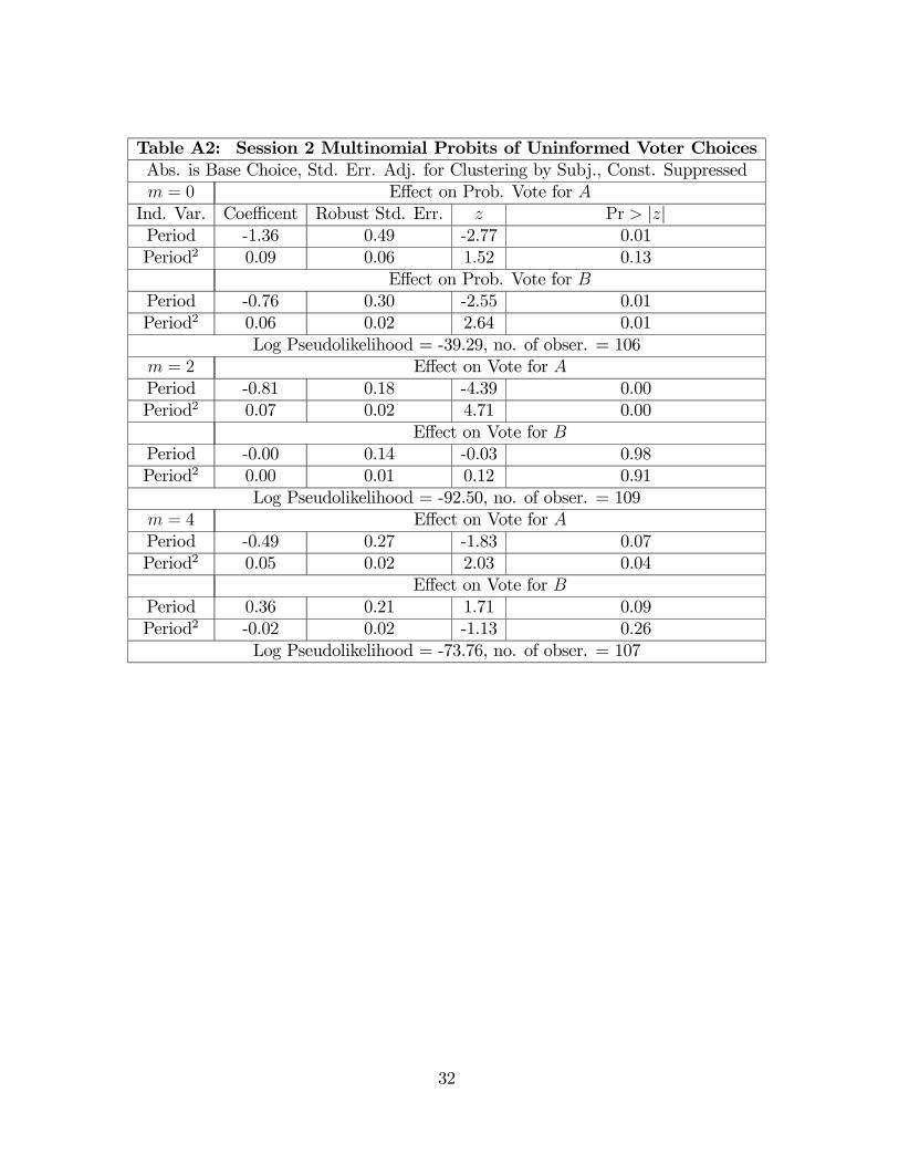
Table A2: Session 2 Multinomial Probits of Uninformed Voter ChoicesAbs. is Base Choice, Std. Err. Adj. for Clustering by Subj., Const. Suppressedm = 0 Effect on Prob. Vote for AInd. Var. Coefficent Robust Std. Err. z Pr > |z|Period -1.36 0.49 -2.77 0.01Period2 0.09 0.06 1.52 0.13
Effect on Prob. Vote for BPeriod -0.76 0.30 -2.55 0.01Period2 0.06 0.02 2.64 0.01
Log Pseudolikelihood = -39.29, no. of obser. = 106m = 2 Effect on Vote for APeriod -0.81 0.18 -4.39 0.00Period2 0.07 0.02 4.71 0.00
Effect on Vote for BPeriod -0.00 0.14 -0.03 0.98Period2 0.00 0.01 0.12 0.91
Log Pseudolikelihood = -92.50, no. of obser. = 109m = 4 Effect on Vote for APeriod -0.49 0.27 -1.83 0.07Period2 0.05 0.02 2.03 0.04
Effect on Vote for BPeriod 0.36 0.21 1.71 0.09Period2 -0.02 0.02 -1.13 0.26
Log Pseudolikelihood = -73.76, no. of obser. = 107
32
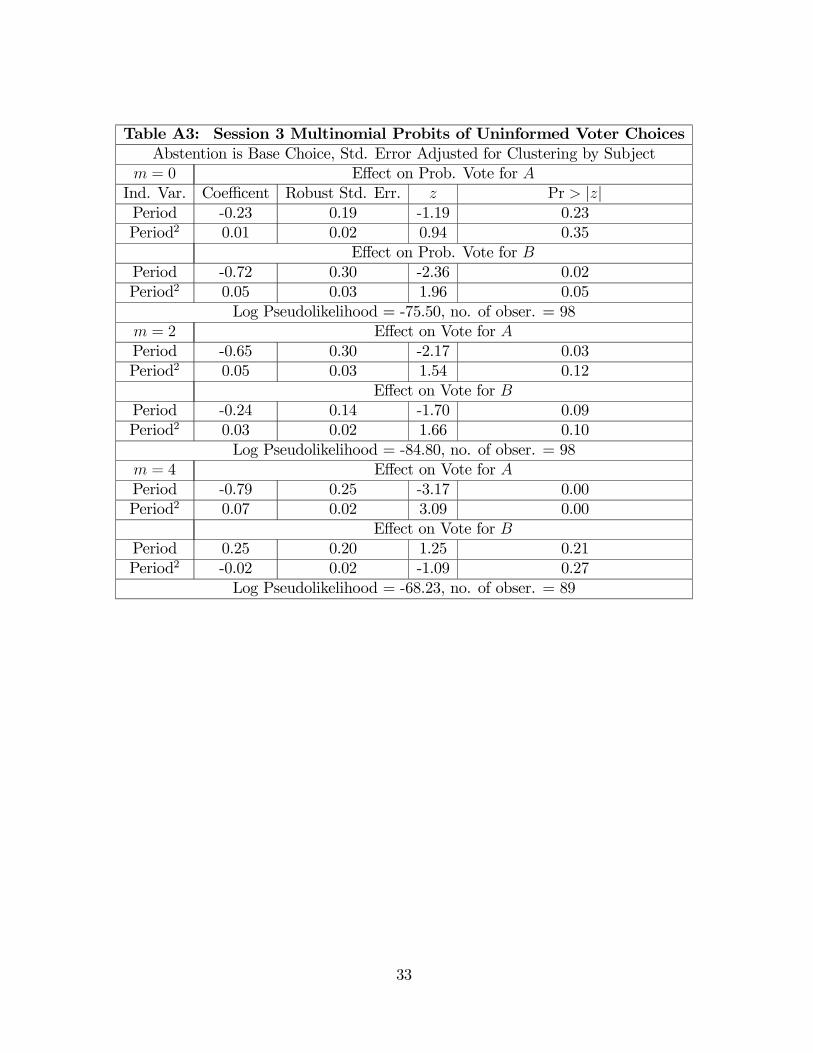
Table A3: Session 3 Multinomial Probits of Uninformed Voter ChoicesAbstention is Base Choice, Std. Error Adjusted for Clustering by Subject
m = 0 Effect on Prob. Vote for AInd. Var. Coefficent Robust Std. Err. z Pr > |z|Period -0.23 0.19 -1.19 0.23Period2 0.01 0.02 0.94 0.35
Effect on Prob. Vote for BPeriod -0.72 0.30 -2.36 0.02Period2 0.05 0.03 1.96 0.05
Log Pseudolikelihood = -75.50, no. of obser. = 98m = 2 Effect on Vote for APeriod -0.65 0.30 -2.17 0.03Period2 0.05 0.03 1.54 0.12
Effect on Vote for BPeriod -0.24 0.14 -1.70 0.09Period2 0.03 0.02 1.66 0.10
Log Pseudolikelihood = -84.80, no. of obser. = 98m = 4 Effect on Vote for APeriod -0.79 0.25 -3.17 0.00Period2 0.07 0.02 3.09 0.00
Effect on Vote for BPeriod 0.25 0.20 1.25 0.21Period2 -0.02 0.02 -1.09 0.27
Log Pseudolikelihood = -68.23, no. of obser. = 89
33

Table A4: Session 4 Multinomial Probits of Uninformed Voter ChoicesAbstention is Base Choice, Std. Error Adjusted for Clustering by Subject
m = 0 Effect on Prob. Vote for AInd. Var. Coefficent Robust Std. Err. z Pr > |z|Period -0.41 0.24 -1.71 0.09Period2 0.01 0.02 0.50 0.62
Effect on Prob. Vote for BPeriod -0.62 0.14 -4.50 0.00Period2 0.05 0.01 3.60 0.00
Log Pseudolikelihood = -63.13, no. of obser. = 105m = 2 Effect on Vote for APeriod -0.69 0.20 -3.42 0.00Period2 0.06 0.02 3.31 0.00
Effect on Vote for BPeriod -0.37 0.18 -2.06 0.04Period2 0.03 0.02 1.89 0.06
Log Pseudolikelihood = -87.29, no. of obser. = 107m = 4 Effect on Vote for APeriod -0.78 0.25 -3.10 0.00Period2 0.07 0.02 3.68 0.00
Effect on Vote for BPeriod 0.06 0.16 0.40 0.69Period2 -0.01 0.01 -0.46 0.65
Log Pseudolikelihood = -99.39, no. of obser. = 117
VII.6 Experiment instructions for one of the sessions
Thank you for agreeing to participate in this experiment. This is an experiment in group
decision making. During the experiment we require your complete, undistracted attention
and ask that you follow instructions carefully. Please turn off your cell phones. Do not
open other applications on your computer, chat with other students, or engage in other
distracting activities, such as reading books, doing homework, etc. You will be paid
for your participation in cash, at the end of the experiment. Different participants may
earn different amounts. What you earn depends partly on your decisions, partly on the
decisions of others, and partly on chance. The entire experiment will take place through
computer terminals. It is important that you not talk or in any way try to communicate
with other participants during the experiments.
The experiment you are participating in is a group decision making experiment, where
you will be making decisions in committees. We will start with a brief instruction period.
During the instruction period, you will be given a complete description of the experiment
34

and will be shown how to use the computers. If you have any questions during the
instruction period, please raise your hand and your question will be answered out loud
so everyone can hear. If you have any questions after the experiment has begun, raise
your hand, and an experimenter will come and assist you. The practice session will be
followed by the paid session. At the end of the paid session, you will be paid the sum of
what you have earned, plus a show-up fee of $10.00. Everyone will be paid in private and
you are under no obligation to tell others how much you earned. Your earnings during
the experiment are denominated in FRANCS. Your DOLLAR earnings are determined
by multiplying your earnings in FRANCS by a conversion rate. For this experiment the
conversion rate is 0.01, meaning that 100 FRANCS equal 1 DOLLAR. The computer
keeps a record of the payments, but you are also asked to keep track of your earnings on
a record sheet.
For the entire experiment, there will be a monitor, who will be chosen from one of the
participants in this room. The monitor will assist in running the experiment by rolling
a die and generating random numbers for use in the experiment and will be paid a fixed
amount ($20.00) for the experiment. [Select monitor] The monitor is the participant who
is seated in front of computer #XX. Please go to Computer # 21. Please continue to pay
attention to the Instructions as they are also relevant to you. If you have any questions,
please ask. If you should have questions once the experiment has started, please ask the
assistant sitting next to you. We will now begin a brief instruction period followed by a
practice session. You will not be paid for the practice session. After the practice session,
there will be a short comprehension quiz, and all questions must be answered correctly
before continuing to the paid session.
Part 1
This experiment has 3 parts. The first part of the experiment will take place over a
sequence of 10 matches. We begin the first match by dividing you into 2 committees of
seven members each. Each of you is assigned to exactly one of these committees. You are
not told the identity of the other members of your committee.
Your committee will make one of two decisions. The decision is simply a choice
between one of two “jars”, the Red Jar or the Yellow Jar. Committees make decisions
by voting. Whichever jar receives more votes is the committee’s decision, and ties are
broken randomly. At the beginning of the match, the monitor secretly rolls a 10-sided die
to determine which of the two jars is the correct jar for your committee, and enters this
information into the master computer. If the die rolled by the monitor comes up 1, 2, 3,
4 or 5 then the Red Jar is the correct jar for your committee; if the die comes up 6, 7, 8
or 9, the Yellow Jar is the correct jar for your committee. If the die comes up a 10, then
it will be rolled again until one of the first 9 numbers comes up. Therefore, in each match
35
there is a 5 out of 9 chance your committee’s correct jar is Red and a 4 out of 9 chance it
is Yellow. The die is rolled separately for each committee, and separately for each match.
The color of your committee’s jar is then recorded in the computer. You will not be told
which jar is the correct decision until after all the members in your committee have voted.
Before voting, each of you receive a piece of information that may or may not help you
decide which is the correct jar. We will describe this information in a moment.
Payoffs are determined as follows. If your committee decision is the correct jar, every-
one in your committee receives a high payoff equal to 80 francs. If your committee decision
is not the correct jar, everyone in the committee receives a low payoff equal to 5 francs.
After receiving this piece of information, you must either vote of one of the two jars
or abstain. Ties (0-0, 1-1, 2-2, 3-3) are broken randomly. So, for example if three of
the seven members of the committee voted for yellow jar, three voted for red jar, and 1
member abstained, then the total vote would be 3-3, which is a tie, and the tie would be
broken randomly. After everyone in your committee has made their decisions to either
vote or abstain, you are told the group decision, exactly what the total votes were, and the
correct jar is revealed to you. If your committee’s group decision is equal to the Correct
jar, each member of your committee earns 80 francs. If your committee’s group decision
is incorrect, each member of your committee earns 5 francs. The other committees in the
room face similar tasks, but the correct decision may be different for different committees.
Remember that committees are completely independent, and they act independently.
After the first match is completed, we proceed to the second match and the process
repeats itself. This will continue for a total of 10 matches. After 10 matches, the first
part of the experiment will be complete and we will read you instructions for the second
part.
From now on the experiment will take place through computer terminals only, except
for the roll of the die performed by the monitor.
We will now begin a Practice session and go through one practice match. During
the practice match, please do not hit any keys until you are asked to, and when you are
instructed to enter information, please do exactly as asked. Again, you are not paid for
this practice match.
[AUTHENTICATE CLIENTS]
Please double click on the icon on your desktop that says s-v-c. When the computer
prompts you for your name, type your First and Last name. Then click SUBMIT and
wait for further instructions.
[SCREEN 1]
You now see the first screen of the experiment on your computer. It should look
similar to this screen. [POINT TO PPT SLIDE DISPLAYED ON SCREEN IN FRONT
36

OF ROOM] Please note that the screen exhibited up front is not necessarily exactly
identical to the screen exhibited on your computer at this time. All the slides we display
in front are just to illustrate.
At the top left of the screen, you see your subject ID. [POINT and mention that your
subject number may be different] Please record that on your record sheet now. You have
been assigned by the computer to a group of 7 subjects. This committee assignment will
change after each match.
On the upper right of your screen there are pictures of two jars, each containing exactly
12 balls. The Red Jar contains 3 Red balls and 9 White balls. The Yellow Jar contains 3
Yellow balls, and 9 White balls.
The monitor will now roll a die, to determine a jar for each committee for this match
and will enter this information into the computer. The Jar for a committee represents
that committee’s correct decision. The die is rolled separately for each committee. As a
result, either Jar may be the correct Jar for each committee.
As I said before, different committees may have been assigned different Jars. You will
not be told which Jar was assigned to your committee until everyone in your committee
has chosen to vote or Abstain. Before you make your choice, each of you is allowed to
see a small piece of information that may or may not help you determine which jar was
assigned to your group. Please wait... we will explain this shortly.
[PUT UP TABLE WITH PAYOFFS]
If you look at the screen in the front of the room, it shows how your payoff is de-
termined. If your committee’s decision matches the committee’s actual Jar, you earn 80
francs for the match and you earn 5 francs if the group decision does not match the actual
Jar. [GO THROUGH EACH LINE ON THE TABLE]
[SCREEN 2]
After the monitor has rolled the die for each committee to determine that committee’s
correct jar, and the information has been entered into the master computer, you will see
this screen. You now see only one jar on your screen, but the colors of the balls are hidden
so at this point you cannot tell which jar it is. This jar is your committee’s correct jar. If
it is a red jar, then there are 3 red balls and 9 white balls; if it is a yellow jar, then there
are 3 yellow balls and 9 white balls.
(Emphasize and repeat later) Please note that the balls have been randomly shuffled
on each of your screens by the computer so there is no way to guess which color ball is in
which location and you cannot tell which Jar was assigned to your committee.
You will now be allowed to see the color of exactly one of the balls in your committee’s
jar. To do so, now please use the mouse to move your cursor to whichever ball you want
to look at and click once.
37

[SHOW SCREEN 3]
We call this ball “your sample”. It is your piece of private information. The other
members of your committee are also choosing balls in a similar way, although the locations
of their balls were shuffled differently for each subject. Therefore, different members of the
same committee may be clicking on different color balls even from the same jar. However,
if the jar is the red jar, then only red and white balls are possible, and if the jar is the
yellow jar, then only yellow and white balls are possible. The colors of all the other balls
remain hidden until the end of the match. Please record the color of your sample on your
record sheet (R for red or Y for Yellow or W for White).
Since the Red Jar has no yellow balls and the Yellow Jar has no red balls, this means
that if you picked a red ball, your committee’s jar must be the Red Jar, and if you picked
a yellow ball, your committee’s jar must be the Yellow Jar. Also since 9 of the 12 balls
in each jar are white, drawing a white ball gives you no useful information about your
committee’s Jar.
We now move to the voting stage.
At this point you will have an opportunity to either vote for the Red Jar, vote for the
Yellow Jar, or Abstain. Since this is a practice match, we are not going to let you choose,
but instead ask that you vote according to your id number. If your ID number is between
0 and 5 (7 IF 21 SUBJECTS), vote for Red. If your ID number is between 6 and 10 (8
AND 14 IF 21 SUBJECTS), vote for Yellow. If your ID number is between 11 and 14,
Abstain. Of course, during the paid matches, you will be making your own decisions.
Once everyone has voted or abstained, you are told the committee decision and your
committee’s jar is revealed to you on this screen.
[SHOW SCREEN 4]
This final screen also displays the correct jar for your committee, your committee’s
decision, how many votes each Jar received and how many voters in your committee
abstained. Also, please note that at the end of the match the colors of all the balls in
your jar are revealed to you. This marks the end of the match.
Now we are ready for the short comprehension quiz. Everyone must answer all the
questions correctly before we go to the paid matches. Also, during the quiz, you must
answer all the questions on Page 1 of the quiz to proceed to Page 2 and 3. If you answer
a question incorrectly, you will be asked to correct it. Please raise your hand if you have
any questions during the quiz, and we will come to your desk and answer your question
in private.
[SHOW SCREEN 5]
Your total payoff is displayed. Please click on the “OK” button to finish the match.
[SHOW SCREEN 6]
38

The table with columns in the bottom of your screen is the History panel and sum-
marizes all of this important information.
[AS YOUREADTHEFOLLOWINGPARAGRAPH, POINTTORELEVANTCOLUMNS
ON THE SCREEN IN FRONT]
COLUMN ONE indicates the match number, COLUMN TWO indicates your sample
color, COLUMN THREE shows your vote, COLUMN four provides a summary of the
votes: (Red Jar- Yellow Jar -Abstention), COLUMN FIVE shows your committee’s de-
cision, COLUMN SIX shows the what the actual jar was, and COLUMN SEVEN shows
your earnings (which are not listed here because this was a practice session).
Now, please make sure you have recorded all the information for this practice match
on your record sheet. You must record this after each match.
In summary, please remember the following important things. The committee decision
is made by plurality rule. Whichever jar receives more votes is the committee decision,
with ties broken randomly by the computer. Committee decisions are summarized in the
text in the upper left panel of your screen (POINT), and are also summarized in the
history screen at the bottom in column five (POINT). As the experiment proceeds the
history screen will gradually list information about all the previous committees you were
in.
[DISPLAY NEW SLIDE WITH SUMMARY INFORMATION and summarize it by
pointing]
[START GAME]
Are there any questions before we begin with the paid session?
[WAIT FOR QUESTIONS]
We will now begin with the 10 paid matches of the first part of the experiment,
remember there are 3 parts in this experiment. We will explain the instructions for part
2 after part 1 is finished and will read the instructions for part 3 after part 2 is finished.
Please pull out your dividers for the paid session of the experiment. If there are any
problems or questions from this point on, raise your hand and an experimenter will come
and assist you.
[DO NOT USE AUTO ADVANCE MATCHES. AFTER MATCH 10 (server) READ
THE FOLLOWING NEW INSTRUCTIONS]
Part 2
This completes part 1. Part 2 is almost exactly the same as part 1, with one exception.
The computer plays the role of two additional members of your committee. Those two
computerized members of your committee always vote for the red jar no matter what. As
before, your committee’s decision is made by plurality rule. Whichever jar receives more
votes, including the two red jar votes from the computer, is your committee’s decision.
39
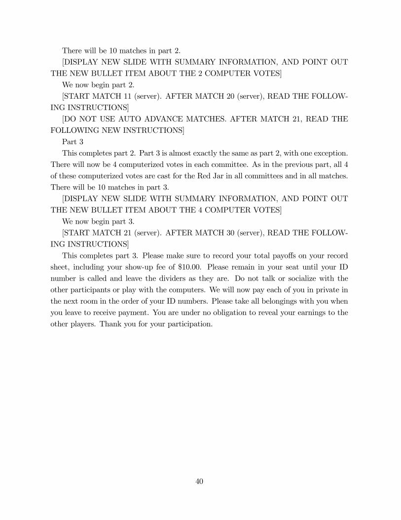
There will be 10 matches in part 2.
[DISPLAY NEW SLIDE WITH SUMMARY INFORMATION, AND POINT OUT
THE NEW BULLET ITEM ABOUT THE 2 COMPUTER VOTES]
We now begin part 2.
[START MATCH 11 (server). AFTER MATCH 20 (server), READ THE FOLLOW-
ING INSTRUCTIONS]
[DO NOT USE AUTO ADVANCE MATCHES. AFTER MATCH 21, READ THE
FOLLOWING NEW INSTRUCTIONS]
Part 3
This completes part 2. Part 3 is almost exactly the same as part 2, with one exception.
There will now be 4 computerized votes in each committee. As in the previous part, all 4
of these computerized votes are cast for the Red Jar in all committees and in all matches.
There will be 10 matches in part 3.
[DISPLAY NEW SLIDE WITH SUMMARY INFORMATION, AND POINT OUT
THE NEW BULLET ITEM ABOUT THE 4 COMPUTER VOTES]
We now begin part 3.
[START MATCH 21 (server). AFTER MATCH 30 (server), READ THE FOLLOW-
ING INSTRUCTIONS]
This completes part 3. Please make sure to record your total payoffs on your record
sheet, including your show-up fee of $10.00. Please remain in your seat until your ID
number is called and leave the dividers as they are. Do not talk or socialize with the
other participants or play with the computers. We will now pay each of you in private in
the next room in the order of your ID numbers. Please take all belongings with you when
you leave to receive payment. You are under no obligation to reveal your earnings to the
other players. Thank you for your participation.
40

References
[1] Austen-Smith, David and Banks Jeffrey, 1996. Information Aggregation, Rationality,
and the Condorcet Jury Theorem. American Political Science Review. 90, pp. 34-45.
[2] Battaglini, Marco. 2005. Sequential Voting with Abstention. Games and Economic
Behavior, 51 (2), pp. 445-63.
[3] Battaglini, Marco, Rebecca Morton, and Thomas Palfrey. 2005. Efficiency, Equity,
and Timing in Voting Mechanisms. Working Paper. Center for the Study of Demo-
cratic Politics. Princeton University.
[4] Cason, Timothy and V.-L. Mui, 2005. Uncertainty and resistance to reform in labo-
ratory participation games. European Journal of Political Economy. In Press.
[5] Crain, W. Mark, Donald R. Leavens, and Lynn Abbot. 1987. Voting and Not Voting
at the Same Time. Public Choice, 53, pp. 221-29.
[6] Coate, Stephen and Michael Conlin. 2004. A Group Rule-Utilitarian Approach to
Voter Turnout: Theory and Evidence," American Economic Review. 94(5), pp. 1476-
1504.
[7] Coate, Stephen, Michael Conlin and Andrea Moro, 2004. The Performance of the
Pivotal-Voter Model in Small-Scale Elections: Evidence from Texas Liquor Refer-
enda. Working Paper. Cornell University.
[8] Coupe, Thomas and Abdul Noury. 2004. Choosing not to choose: on the link
between information and abstention, Economics Letters 84, pp. 261—65.
[9] Feddersen, Timothy J. 2004. Rational Choice Theory and the Paradox of Not Voting.
Journal of Economic Perspectives. 18(1). 99-112.
[10] Feddersen, Timothy J. and Pesendorfer Wolfgang, 1996. The Swing Voter’s Curse,
American Economic Review. 86(3), pp. 404-24.
[11] Feddersen, Timothy J. and Pesendorfer Wolfgang, 1997. Voting Behavior and In-
formation Aggregation in Elections with Private Information. Econometrica. 65, pp.
1029-58.
[12] Feddersen, Timothy J. and Pesendorfer Wolfgang, 1999. Absetention in Elections
with Asymmetric Information and Diverse Preferences. American Political Science
Review. 93(2), pp. 381—98.
41

[13] Filer, John, Lawrence Kenny, and Rebecca Morton. 1993. “Redistribution, Income,
and Voting.” American Journal of Political Science, 37, pp. 63-87.
[14] Gentzkow, Matthew. 2005. Television and Turnout. Working paper. University of
Chicago Business School.
[15] Grofman, Brenard. 1993. Is Turnout the Paradox that Ate Rational Choice Theory?
in Information, Participation, and Choice (ed. B. Grofman), University of Michigan
Press: Ann Arbor.
[16] Grosser, Jens, Tamar Kugler and Arthur Schram. 2005. Preference Uncertainty, Voter
Participation and Electoral Efficiency: An Experimental Study.Working Paper, Uni-
versity of Cologne.
[17] Guarnaschelli, Serena, Richard D. McKelvey, and Thomas R. Palfrey, 2000, An Ex-
perimental Study of Jury Decision Rules, American Political Science Review, 94(2),
pp. 407-23.
[18] Hansen, Stephen, Thomas R. Palfrey, and Howard Rosenthal. 1987. The Downsian
Model of Electoral Participation: Formal Theory and Empirical Analysis of the Con-
stituency Size Effect. Public Choice. 52: 15-33.
[19] Kagel, John and Dan Levin. 2002. Common Value Auctions and the Winner’s Curse,
Princeton University Press: Princeton.
[20] Klein, David and Lawrence Baum. 2001. Ballot Information and Voting Decisions
in Judicial Elections. Political Research Quarterly, 54(4), pp. 709-28.
[21] Lassen, David D. 2005. The Effect of Information on Voter Turnout: Evidence from
a Natural Experiment, American Journal of Political Science, 49(1), pp. 103-18.
[22] Ledyard, John O., 1984,The Pure Theory of Large Two-Candidate Elections, Public
Choice, 44, pp. 7-41.
[23] Levine, David K. and Thomas R. Palfrey Palfrey, 2005. The Paradox of Voter Par-
ticipation? Working Paper, Center for the Study of Democratic Politics, Princeton
University.
[24] Matsusaka, John G. 1995. Explaining Voter Turnout Patterns: An Information
Theory. Public Choice, 84, pp. 91-117.
42
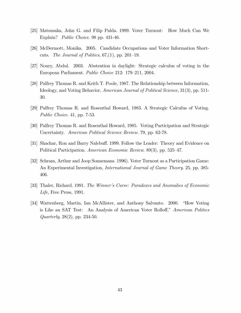
[25] Matsusaka, John G. and Filip Palda. 1999. Voter Turnout: How Much Can We
Explain? Public Choice. 98 pp. 431-46.
[26] McDermott, Monika. 2005. Candidate Occupations and Voter Information Short-
cuts. The Journal of Politics, 67,(1), pp. 201—19.
[27] Noury, Abdul. 2003. Abstention in daylight: Strategic calculus of voting in the
European Parliament. Public Choice 212: 179—211, 2004.
[28] Palfrey Thomas R. and Keith T. Poole, 1987. The Relationship between Information,
Ideology, and Voting Behavior, American Journal of Political Science, 31(3), pp. 511-
30.
[29] Palfrey Thomas R. and Rosenthal Howard, 1983. A Strategic Calculus of Voting.
Public Choice. 41, pp. 7-53.
[30] Palfrey Thomas R. and Rosenthal Howard, 1985. Voting Participation and Strategic
Uncertainty. American Political Science Review. 79, pp. 62-78.
[31] Shachar, Ron and Barry Nalebuff. 1999. Follow the Leader: Theory and Evidence on
Political Participation. American Economic Review. 89(3), pp. 525—47.
[32] Schram, Arthur and Joop Sonnemans. 1996). Voter Turnout as a Participation Game:
An Experimental Investigation, International Journal of Game Theory. 25, pp. 385-
406.
[33] Thaler, Richard. 1991. The Winner’s Curse: Paradoxes and Anomalies of Economic
Life, Free Press, 1991.
[34] Wattenberg, Martin, Ian McAllister, and Anthony Salvanto. 2000. “How Voting
is Like an SAT Test: An Analysis of American Voter Rolloff,” American Politics
Quarterly, 28(2), pp. 234-50.
43


![Vol 39 - [Swing, Swing, Swing]](https://static.fdocuments.net/doc/165x107/55cf8f5a550346703b9b7709/vol-39-swing-swing-swing-5699adb3c742c.jpg)

