The Study ofRelative Density and Boundary Effects

for Cone Penetration Tests inCentrifuge

M. D. Bolton ’ and M. W. Gui 2

CUED/D-SOILS/TR256 1993

‘. Lecturer, Cambridge University Engineering Department, UK.2 . Research Student, Cambridge University Engineering Department, UK.

Abstract

A series of cone penetration tests were carried out at the Cambridge Geotechnical

Centrifuge Centre. The tests were performed using a 1Omm diameter cone penetrometer.

In order to study the effect of diameter ratio, three different sizes of container (210mm,

420mm and 850mm diameter) were used. The repeatability of the model preparation

technique using a single hole hopper was checked prior to these tests. Side boundary and

base boundary effects are found to be significant and a minimum diameter ratio is proposed

for tests to be carried out using a circular container. The effect of the relative density of

Fontainbleau sand is studied. The possibility of simulating an infinite body of sand is

also mentioned. It has also been demonstrated that the relative density of sand can be

correlated with the normalised tip resistance.

Contents

Abstrtact

Table of Contents

List of Figures

Notation

1 Introduction

2 Literature Review

2.1 Calibration chamber tests . . . . . . . . . . . . . . . . . . . . . . . . . . .

2.2 Some remarks about calibration chamber tests . . . . . . . . . . . . . . . .

3 Centrifuge Tests

3.1 Test programme. . . . . . . . . . . . . . . . . . . . . . . . . . . . . . . . .

3.2 Sand properties . . . . . . . . . . . . . . . . . . . . . . . . . . . . . . . . .

3.3 Model preparation . . . . . . . . . . . . . . . . . . . . . . . . . . . . . . .

3.4 Cone penetration testing . . . . . . . . . . . . . . . . . . . . . . . . . . . .

3.4.1 Power system - Pneumatic . . . . . . . . . . . . . . . . . . . . . . .

3.4.2 Power system - Hydraulic . . . . . . . . . . . . . . . . . . . . . . .

4 Analysis of Results

4.1 Penetration mechanisms . . . . . . . . . . . . . . . . . . . . . . . . . . . .

4.2 The effect of relative density, ID . . . . . . . . . . . . . . . . . . . . . . . .

4.3 The effect of side boundary . . . . . . . . . . . . . . . . . . . . . . . . . .

4.4 The effect of base boundary . . . . . . . . . . . . . . . . . . . . . . . . . .

4.5 Base boundary pressure during penetration . . . . . . . . . . . . . . . . . .

4.6 Correlation between normalised qc and ID . . . . . . . . . . . . . . . . . .

5 Conclusion

Acknowledgement

References

i

ii

i v

1

8

8

8

8

1 0

1 1

1 1

14

1 4

1 7

17

1 8

2 1

22

25

26

27

i i

List of Figures

1

2

3

4

5

6

7

8

9

1 0

1 1

1 2

1 3

1 4

1 5

1 6

1 7

1 8

Chamber size effects on qc (after Parkin & Lunne, 1982) . . . . . . . . . . 2

Variation of qc with diameter ratio (after Last, 1979) . . . . . . . . . . . . 3

Comparison of qc profiles for OC sand in calibration and rigid-walled chambers 5

Tip resistance profiles (after Phillips and Valsangkar, 1987) . . . . . . . . . 6

Vertical stress fields around cone in the field and chamber . . . . . . . . . 7

Assembles of centrifuge package . . . . . . . . . . . . . . . . . . . . . . . . 9

Particle size distribution curve for Fontainbleau sand . . . . . . . . . . . . 1 0

Repeatability of sand pouring technique in Cambridge . . . . . . . . . . . 1 1

CUED cone penetrometer . . . . . . . . . . . . . . . . . . . . . . . . . . . 1 2

Hydraulic system on centrifuge arm . . . . . . . . . . . . . . . . . . . . . . 1 3

Tip resistance profiles . . . . . . . . . . . . . . . . . . . . . . . . . . . . . . 1 5

Normalised tip resistance profiles . . . . . . . . . . . . . . . . . . . . . . . 1 6

Definition of critical depth . . . . . . . . . . . . . . . . . . . . . . . . . . . 17

Relationship between Q= and diameter ratio, 5 . . . . . . . . . . . . . . . . 1 9

Base boundary effect for Fontainbleau sand @ 70g . . . . . . . . . . . . . . . 20

Pressure recorded as the penetrometer advancing . . . . . . . . . . . . . . 2 1

Belationship between ID and normalised Q= . . . . . . . . . . . . . . . . . . 23

Comparison of the estimated ID profiles . . . . . . . . . . . . . . . . . . . 24

. . .111

Notation

B

d

D

9

ID

K

L

n

N C

OC

OCR

I4

PO

Qc

R*

X

&n

ZPC

z

4 crit

4

“Yd

7W

diameter of the cone

mean particle diameter

diameter of container

earth’s gravity(9.81m/s2)

relative density

coefficient of earth pressure

distance of cone from the total stress cell

ratio between centrifugal acceleration and earth’s gravity

normally consolidated

overconsolidated

overconsolidation ratio

soil particle crushing strength

cant ainer pressure

measured tip resistance

radius at the surface of the specimen

distance of cone from the base of the container

depth in the model from the surface to the specimen

corrected prototype depth

normalized prototype depth

critical angle of shearing

initial effective vertical stress

initial total vertical stress

dry density of soil

density of water

iv

1 Introduction

Cone penetration test (CPT) has b een widely used in the last twenty years as an site

investigation tool. It is a relatively simple test and capable of providing a continuous

profile of a site. In order to obtain the engineering parameters from the raw data, laboratory

calibration of CPT data, using calibration chambers, is necessary. To simulate the effect

of the overburden pressure, a surcharge is used. However, the effect of stress gradient due

to the self-weight of the soil cannot be simulated in this way. Hence, the results obtained

from calibration chamber always leave room for questioning.

To simulate the effect of self-.weight, centrifuge testing has been adopted for all sorts

of geotechnical problems. A specimen of soil is prepared in a strongbox in the laboratory,

instrumented and transferred carefully to the centrifuge for testing. A collaboration ex-

ists between European centrifuge centers at Bergamo, Bochum, Copenhagen, Names and

Cambridge, to standardize methods of in-flight site investigation in centrifuge models.

Bolton et al (1993) h ave demonstrated the importance of having miniature probes to

measure in-flight soil parameters, Therefore, a data bank for in-flight CPT will be very

useful when correlations of soil parameters are required.

A series of CPT have, therefore, been conducted at the Cambridge Geotechnical Cen-

trifuge centre. The objective of this report is to study the effects of the relative density

ID, the diameter ratio $$ (container diameter to the cone diameter), and the similar base

boundary effect, on the tip resistance Q= of CPT. For this purpose, the cone tip resistance

qc is normalised with respect to overburden pressure, and the current depth is normalised

with respect to cone diameter.

2 Literature Review

Hitherto, except for Ferguson and Ko (1981), Phillips and Valsangkar (1987) and Lee

(1990), most of the cone data were calibrated from calibration chambers. Different bound-

ary conditions in calibration chambers can be simulated by varying the lateral pressures

around the circumference of the chamber via a rubber membrane. In order to study the

1

W. Loose

I

.+ +,

c+ = 30 %

I I20 50 11

Diameter Raho Rd

0

Figure 1: Chamber size effects on qc (after Parkin & Lunne, 1982)

boundary effects, different sizes $of calibration chamber and different diameters of cone

were adopted. The boundary effects for calibration chamber tests have been studied by

some researchers (eg. Last (1979), Parkin & Lunne (1982) and Ghiona (1984)) and are

summarised in the following section.

2.1 Calibration chamber tests

Parkin and Lunne (1982) investigated boundary effects in flexible-walled chambers. The

tests were preformed using cones with different diameters B in calibration chambers with

different sizes D. The boundary conditions on the flexible side and base were either con-

stant volume B3 or constant stress Bl and the results were plotted in terms of tip resistance

qc and diameter ratio (g) in Fig Il. It was concluded that for loose sand (10 = 15 - 30%),

the boundary effects are negligible and for NC dense sand (10 = 90%), a diameter ratio of

about 50 is desirable in order to eliminate the boundary effects.

2

DENSE NC 032 0 0 -2 0 0 -

100100DENSE OC Bl /DENSE OC Bl /

300- \ - RIGID

1 T LOOSELOOSE TT10 I I

3’0 QL3 II

D I A M E T E R R A T I O 2D I A M E T E R R A T I O 2

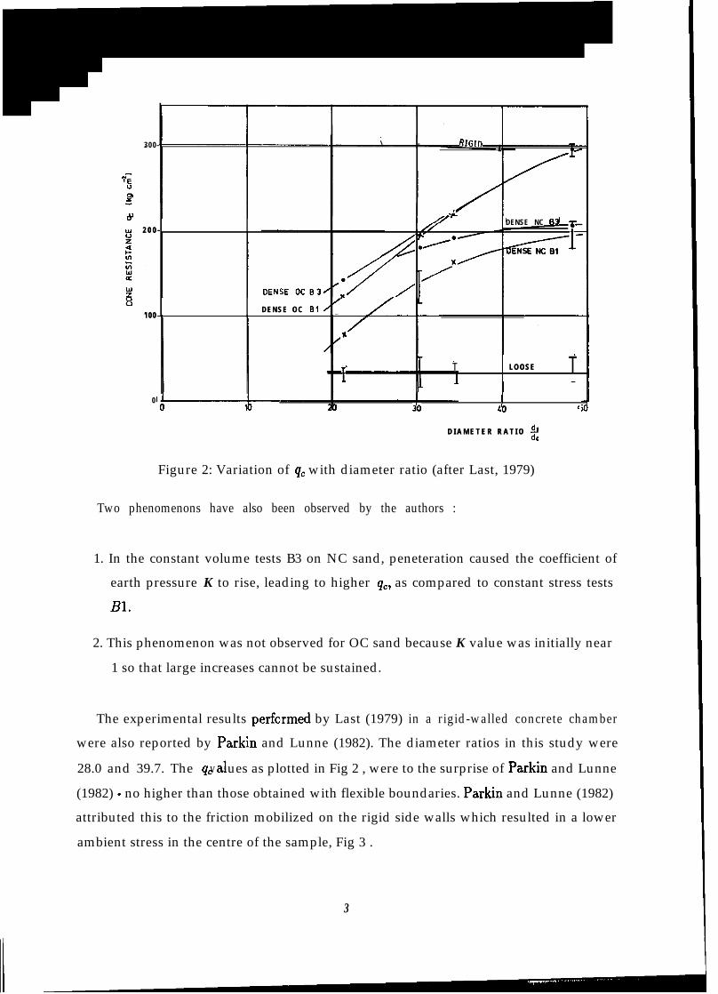
Figure 2: Variation of qc with diameter ratio (after Last, 1979)

Two phenomenons have also been observed by the authors :

1. In the constant volume tests B3 on NC sand, peneteration caused the coefficient of

earth pressure K to rise, leading to higher q. as compared to constant stress tests

Bl.

2. This phenomenon was not observed for OC sand because K value was initially near

1 so that large increases cannot be sustained.

The experimental results perfo’rmed by Last (1979) in a rigid-walled concrete chamber

were also reported by Parkin and Lunne (1982). The diameter ratios in this study were

28.0 and 39.7. The qc alv ues as plotted in Fig 2 , were to the surprise of Parkin and Lunne

(1982) - no higher than those obtained with flexible boundaries. Parkin and Lunne (1982)

attributed this to the friction mobilized on the rigid side walls which resulted in a lower

ambient stress in the centre of the sample, Fig 3 .

3

Ghiona (1984) hs owed that for dense Ticino sand (10 = 90%), there was no chamber

size effect as observed by Parkin and Lunne (1982). The only explanation offered was that

the material was different from the one used by Parkin and Lunne (1982).

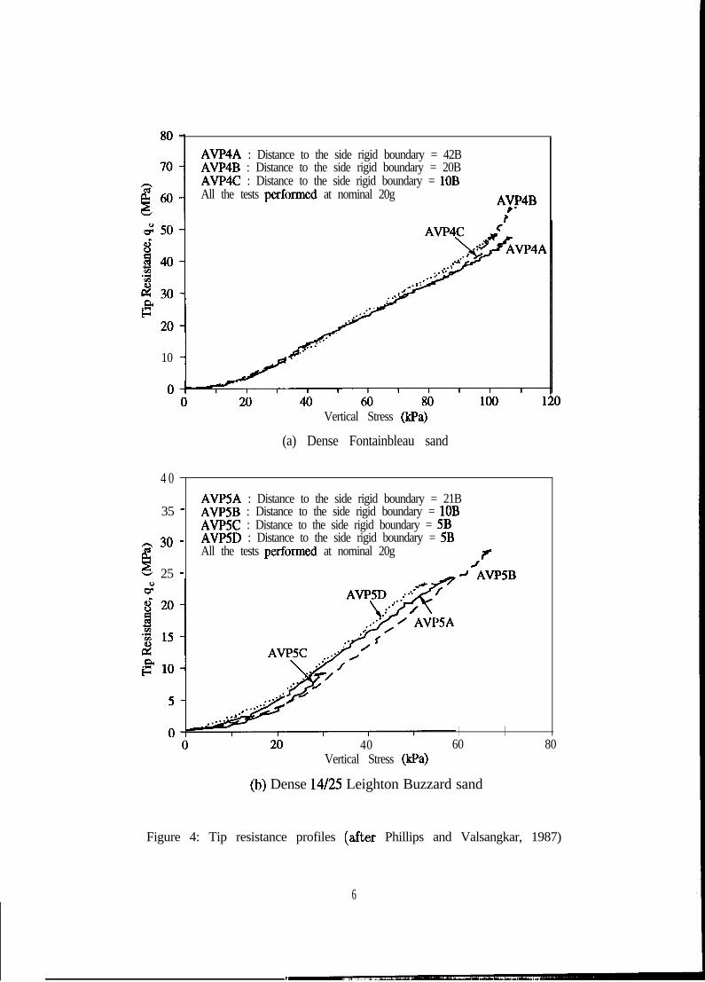
Phillips and Valsangkar (1987) carried out CPT on Fontainbleau and Leighton Buzzard

14/25 sands (ID = 87%) in a 850mm diameter tub. The results of the tests using a cone

with B = 1Omm at distance ratios of lOB, 20B and 42B and tests using a cone with

B = 20mm at distance ratios of 5B, 10B and 21B are presented in Fig 4 (a) & (b).

It was concluded that side wall boundary effects are negligible in the current centrifuge

setup. Small variations in the test results may be due to stress cycling caused by stoppage

of centrifuge between tests. However, Phillips and Valsangkar (1987) recommended that

care has to be taken in extrapolating cone results when more than one side-wall is close to

the penetrometer.

2.2 Some remarks about calibration chamber tests

There are some uncertainties for the tests performed in the calibraton chambers :

1. Parkin and Lunne (1982) bo served the variation of container pressure, PO, throughout

the penetration test. If they normalised qC with respect to P, and plotted E instead,

would they have observed any normalised boundary effect ?

2. Constant volume in a triaxial cell chamber does not mean zero strain everywhere

(cr#O). Hence, “constant volume” chamber tests will be much more compliant at

the boundary than centrifuge tests.

3. The data obtained by Last (1979) and Parkin and Lunne (1982) seem not to explain

qc = f(z,,) very convincingly, Fig 3. It is believed that the initial portion of the

curve could be due to the top boundary effect.

4. For tests carried out in a flexible-walled chamber, the constant stress boundary con-

dition Bl will underestimate gc as higher values will develop in the field or centrifuge

at the equivalent distance from the cone.

4

C3NE R E S I S T A N C E QC (kghn’)

IPENETR~METE~ aoL

I LR

5 815 63

10 8110 83

5 RIGID10 R I G I D

Figure 3: Comparison of qc profiles for OC sand in calibration and rigid-walled chambers

AVP4A : Distance to the side rigid boundary = 42BAVP4B : Distance to the side rigid boundary = 20BAVP4C : Distance to the side rigid boundary = 1OBAll the tests performed at nominal 20g AV$4B

?

10

Vertical Stress @Pa)

(a) Dense Fontainbleau sand

4 0AVPSA : Distance to the side rigid boundary = 21B

35 - AVPSB : Distance to the side rigid boundary = 1OBAVPSC : Distance to the side rigid boundary = 5B

~ 30 - AVPSD : Distance to the side rigid boundary = 5B

si

All the tests pefixmed at nominal 20g f

25 - d /AVPSB

I I40 60 80

Vertical Stress @Pa)

(b) Dense 14/25 Leighton Buzzard sand

Figure 4: Tip resistance profiles (after Phillips and Valsangkar, 1987)

6

- - - - 6, approx. constantI in field

.ifimnt 01

D

In stressf cone

h

Qc* 44 Average verticalstress behind

r - cone tip less1I

than applied 0”I.:.:.:. I:::::::$$g I.A.. . . ..:+>::::::::::::::;:;;g:::.:.:jij$j ;

;$g qc- AC#$- *::::::: Ch::::::::::::::jjjjjjj:::::::::::::::>;:

6, constant in chamber

Applied CJT, constant

(b) Chamber(a) Field/centrifuge

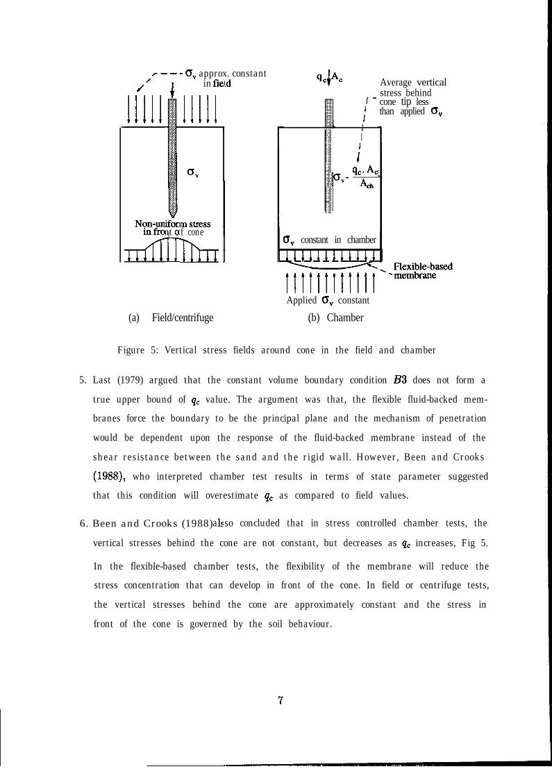
Figure 5: Vertical stress fields around cone in the field and chamber

5. Last (1979) argued that the constant volume boundary condition B3 does not form a

true upper bound of qc value. The argument was that, the flexible fluid-backed mem-

branes force the boundary to be the principal plane and the mechanism of penetration

would be dependent upon the response of the fluid-backed membrane instead of the

shear resistance between the sand and the rigid wall. However, Been and Crooks

(1988), who interpreted chamber test results in terms of state parameter suggested

that this condition will overestimate qc as compared to field values.

6. Been and Crooks (1988) 1,a so concluded that in stress controlled chamber tests, the

vertical stresses behind the cone are not constant, but decreases as qc increases, Fig 5.

In the flexible-based chamber tests, the flexibility of the membrane will reduce the

stress concentration that can develop in front of the cone. In field or centrifuge tests,

the vertical stresses behind the cone are approximately constant and the stress in

front of the cone is governed by the soil behaviour.

3 Centrifuge Tests

10 tests were conducted in the centrifuge to study the relative density and boundary

effects for CPT. The tests were performed using a cone with diameter B = 1Omm and in

3 difference containers with diameter D = 850mm,420mm and 210mm. The assembled

package for centrifuge test and layout of the test location are shown in Fig 6.

3.1 Test programme

The detail and geometry of the tests are tabulated in Table 1.

3.2 Sand properties

Fontainbleau sand, imported from France, was used in the above tests. The particle size

distribution has been determined in accordance with BS 1377:1975; clause 2.7.1. The

distribution curve is presented in Fig 7.

The measured &,-, of the Fontainbleau sand is O.Mmm, where D5c is the grain diameter

at which 50% of the soil weight is finer. I& and Drc are 0.191 and 0.113 respectively.

Hence, the coefficient of uniformity C, (=Dso/Dlo) of the sand is 1.69. Specific gravity G,

of Fontaibleau sand has also been determined using the method prescribed in BS 1377:1975;

clause 2.6.2. The average G, value is 2.644. These values compared reasonably well to the

values obtained by Shi (1988). The sand has a maximum void ratio emaz = 0.92 and

minimum void ratio emin = 0.55.

3.3 Model preparation

The specimen was prepared by raining the Fontainbleau sand from a single hole hopper

into the cylindrical container. The void ratio of the specimen depends on the flow rate and

the height of pouring. To achieve a constant void ratio, the height of the hopper and flow

rate were maintained constant throughout the preparation of specimen. The top surface of

the specimen was then levelled using a suction machine. The repeatability of this technique

rgmCross beam I

1/2D 1/2D

Container(D =L \i 8501

/ *-\/ \

/ \

Setup of smallertub and to besup rtedby

fpsan all round

Figure 6: Assembles of centrifuge package

9

0.1 1 10Particle size (mm)

Figure 7: Particle size distribution curve for Fontainbleau sand

is presented in Fig 8. This method of model preparation can also achieve a fairly uniform

dense specimen.

To avoid a loose sample densifying when disturbed during handling, the sample was

prepared in the centrifuge compound, though shaking as the package goes on the arm is

almost bound to cause some densification. Calculation of void ratio is based on the overall

weight of the specimen and its volume measured after the package had been mounted on

to the centrifuge arm. After each run, the volume of the specimen is measured to ensure

that no significant settlement occurred.

3.4 Cone penetration testing

Basically, there are two power systems involved in CPT in the centrifuge.

1 0

0 4 8 12 16 20 24 2 8Corrected Prototype Depth, zpc (m)

Figure 8: Repeatability of sand pouring technique in Cambridge

3.4.1 Power system - Pneumatic

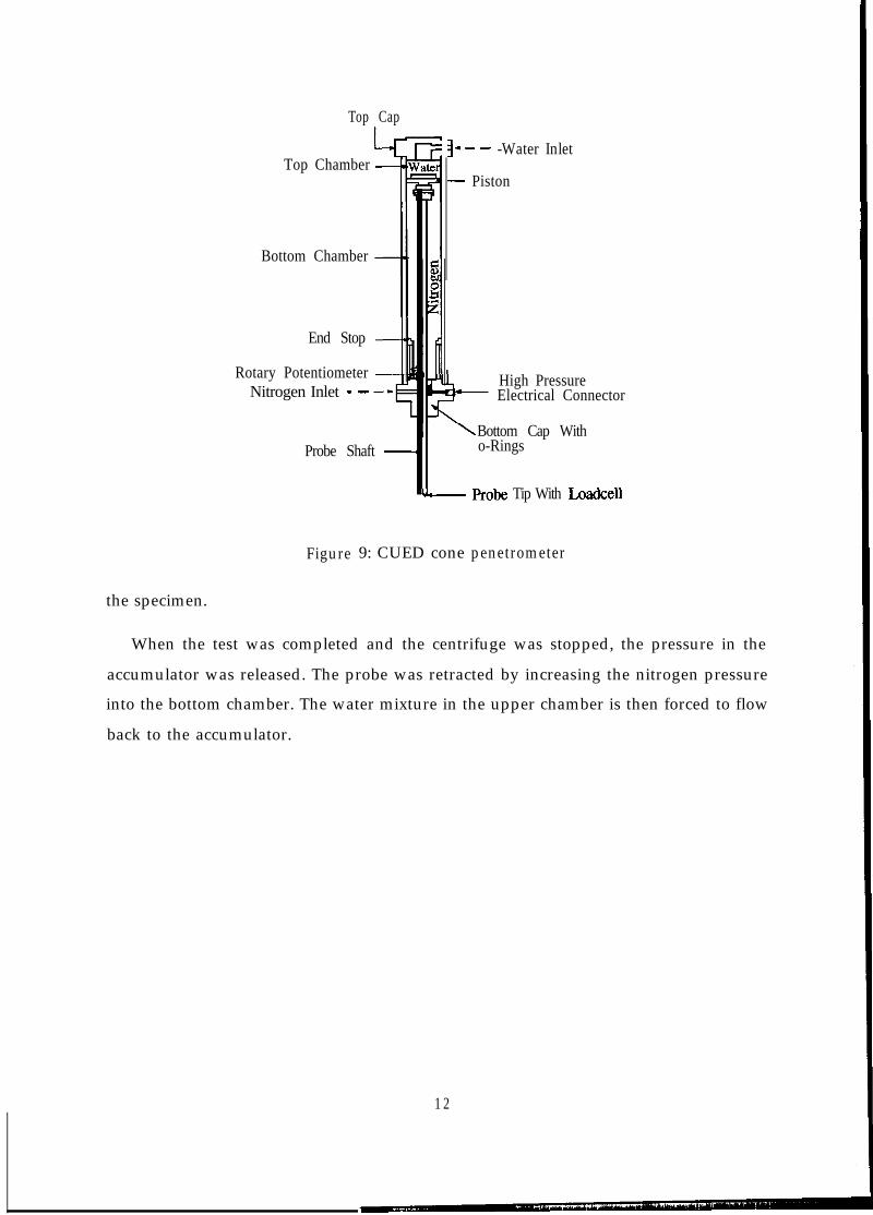
Before the penetration test, during centrifuge flight, nitrogen pressure acting in the bot-

tom chamber is used to prevent the downward movement of the probe and piston under

gravity force, Fig 9. At an acceleration of 7Og, a pressure of about 1200kPa is required to

counteract the weight of the probe and piston and also the head of water in the external

piping. When required, nitrogen can be vented out of the bottom chamber via a pressure

relief valve.

3.4.2 Power system - Hydra.ulic

Fig 10 schematically shows the hydraulic and pressure control systems required during

centrifuge operation of the probe. The hydraulic pressure system is depicted in the top

left hand corner of Fig 10 . The 9.4 litre accumulator contains 4 litres of pressurised water

with additives. By opening the pneumatically actuated 2-way ball valve the pressurised

water will be forced into the top chamber of cone penetrometer, pushing the probe into

11

Top Cap

Top Chamber

Bottom Chamber

End Stop

Rotary PotentiometerNitrogen Inlet - -

Probe Shaft -

Figure

g- - - -Water Inlet

- Piston

High Pressure--- Electrical Connector

Bottom Cap Witho-Rings

G- Prohe Tip With Loadcell

9: CUED cone penetrometer

the specimen.

When the test was completed and the centrifuge was stopped, the pressure in the

accumulator was released. The probe was retracted by increasing the nitrogen pressure

into the bottom chamber. The water mixture in the upper chamber is then forced to flow

back to the accumulator.

1 2

iiiiiiiig

iiI .IT!1%!Iiiiiiiii

Pneumaticallyactuated 2-wayball valve

P /.

Penetrometer

/Nitrogen Pressurecylinders controllers

pressurerelief valve

nn

4 Analysis of Results

Only one CPT was executed for each of the specimen prepared and the location was at the

center of the specimen, Fig 6. The results of CPT are then plotted in the following ways :

1. tip resistance qc versus corrected prototype depth zpc

2. normalized tip resistance Q versus normalized depth of penetration 2

where :

ZPC = ZP.[l + (f&)1Q =yz =%

ZP = a.z,

0, = w.%J1 + ($.$)I

4 = (7 - -b&P54 + ($$-,I

The tip resistance profile for all the tests are plotted in Fig 11 (a) & (b) while the

normal&d tip resistance profile are plotted in Fig 12 (a) & (b). In all cases, the depth,

zm9 is measured from the surface of the test specimens to the shoulder of the cone, Fig 6.

4.1 Penetration mechalnisms

From the normalised plot, Fig 12 (a) & (b), ti is clear that for a complete penetration,

there are two phases of behaviour depending on the depth ratio, 4fp. In the first phase, Q

increases with depth in the fashion of shallow foundations until the so-called critical depth

(Vesic, 1963), Fig 13. Thereafter, the coefficient seems to hold steady or to fall slightly,

which is the characteristic of deep foundations.

The existence of a shallow penetration mechanism requires new correlations in order to

analyse the data obtained from centrifuge models. In the calibration chamber tests, this

mechanism was omitted since most of the data points were recorded at the mid depth of

the sample, well below the critical depth.

1 4

1 I‘G6 88 4 2

MWG9 MWG7 58 54 S! ii: 85 - -MWGS MW,ti5/

, --

0 4 II 12 16 2 0 2 4 2 8Corrected Prototype Depth, zpc (m)

60

MWG9

0 4 I< 12 16 2 0 2 4 2 8Corrected Prototype Depth, zpc (m)

(b)

’ ’

Figure 11: Tip resistance profiles

1 5

5oo’

0 4 8 12 16 2 0 2 4 2 8Norma&d Depth, Z

(a)

- MWGll-MWG12

MWGlO

MWG9

OLl-7 I I I I I I I I I I0 4 8 12 16 2 0 2 4 2 8

Nom-mised Depth, Z

09

Figure 12: Normalised tip resistance profiles

16

Smooth base Rough base

Figure 13: Definition of critical depth

4.2 The effect of relative density, ID

Fig 11 (a) & (b) show that qc is significantly affected by ID. This is because qc is very much

dependent on the mobilised angle of shearing. For a particular stress level, soil with higher

density is always associated with higher mobilised angle of shearing. The CPT profile of

the specimen reveals it is not easy to achieve a consistent density for a specimen with

ID < 60%.

4.3 The effect of side boundary

In order to study the side boundary effect, qc is plotted against i as in Fig 14 (a) & (b).

For very dense Fontainbleau san.d specimens, Fig 14(a), there is no apparent increase in qc

for a test done in 5 = 42, as compared to s = 85. It should be noted that all the density

measurements are accurate to the nearest f2.0%, so we should not be surprised to see

that qc for a nominal density 1~ = 88% appears higher than qc for ID = 89%. However,

Fig 14 (a) shows that qc rose significantly for a test carried out in container with g = 21,

1 7

even though ID = 76%. One may therefore suggest that for dense sand, a minimum Q = 40

is desirable.

Fig 14(b) shows the results obtained from specimens with ID = 54%. Perhaps, more

data are needed in order to study the side boundary effect and also to recommend a

minimum diameter ratio. Nevertheless, the extrapolated profile (dotted line) indicates

that the increment in qc is moderate as compared with very dense specimens.

In this case, the failure mechanism was apparently restrainted by the boundary of the

smaller container, which resulted in higher qc. However, the setup of the test by Phillips

and Valsangkar (1987) was completely different because the probe was placed at 10B

(B = 10mm) from the side wall of a 850mm diameter container. This allowed the failure

mechanism to develope freely on the other side of the probe. This Phillips and Valsangkar

(1987) mechanism was presumably essentially similar to those generated when the probe

was penetrating in the center of a. big tub, except that, it was distorted.

Test MWG12 (ID = 89%) was conducted in a container with Q = 21, Fig 11(b)

and Fig 14 (a). In order to simulate the infinite body of sand, a 3mm thick membrane

(E = 2.75N/mm2) was placed at the circumference of the container. The qc profile fell

nicely on the profile obtained from test MWG5 (ID = 89%, g = 85), except for the last

3m of penetration.

Though the boundary was restrained, the volumetric changes due to the insertion of

probe will be much higher in this setup than the hard boundary condition since the mem-

brane can be deformed easily. An increment in volumetric change means that the soil is

more compressible and it will induce a lower qc value, Vesic (1972).

4.4 The effect of base boundary

A base boundary effect was detected in most of the tests done in the centrifuge (eg. Phillips

and Valsangkar, 1987; Lee, 1990 and Phillips and Gui, 1992). From the above tests, it was

found that the base effect is more significant and obvious in dense specimens (1~ > 80%).

In order to eliminate the base boundary effect, a 3mm thick membrane was placed at the

base of the test container MWG6 and MWG7.

1 8

ID=76%m ,\- -

zpc=20mn

% \

=89n 88

\89. c----u

16m88 n 89

g: ‘i 188- - 12m=89

76 n 4 ‘l-,88 8m89 n a89

extra lated. - -profI e.p” without

: sidemembrane. :76 , - ; -Z _ ~88 4 m89 n 89

!. _ pgfikip side

0 20 40 60 80 1

Diameter ratio, D/B

2826 54. .4

24\ \

2 223 2 0-, 18; 16

314

.9 12

extrapolated profile(without side membrane)

\ \ J,- - =u)m---=.- - - #54

- -- - - - 16mm--v

- - -B54- - - - 12m--_- -B54‘- 8m----__---- =54

J 10

g 86

54m *--- - - -

- - 4 m--___-4 n 54

40 60

Diameter ratio, D/B

(b)

80 100

Figure 14: Relationship between qc and diameter ratio, $$

19

1 0

9

8

7

6

Relative hnSity, ID(%)

Figure 15: Base boundary effect for Fontainbleau sand @ 70g

From Fig 12(a), it can be observed that the base boundary effect for dense specimen in

test MWG6 was not as much as tests MWGSA and MWG5. For loose specimen MWG7

(ID < 54%), th e introduction of a base membrane failed to eliminate the effect. This is

because, while the cone is advancing, the loose sand in front of the cone is densifying all

the time.

The base boundary effect recorded from the tests was found to be influenced signif-

icantly by the relative density of the sand. To find a relationship between these two

parameters, Bx is plotted against ID in Fig 15, where X is the distance from the base of

the container to the shoulder of cone.

The best fitted line through these data points suggested that,

XB = 0.099&a%) + 0.596 (1)

with the coefficient of correlation, R2, between the interpolated line and the data points

being 0.90.

, leakage occurcd vertical stressbefore CPTStarted

\

0-i I I I 1 I I 8 I I I I I 1 I0 4 8 12 16 20 24 28

Distance Ratio (UB) from TSC to cone shoulder

Figure 16: Pressure recorded as the penetrometer advancing

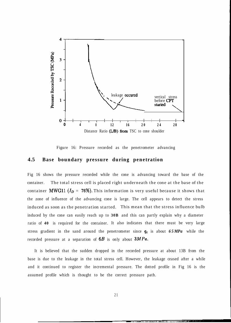
4.5 Base boundary pressure during penetration

Fig 16 shows the pressure recorded while the cone is advancing toward the base of the

container. The total stress cell is placed right underneath the cone at the base of the

container MWGll (10 = 76!?%). This information is very useful because it shows that

the zone of influence of the advancing cone is large. The cell appears to detect the stress

induced as soon as the penetration started. This mean that the stress influence bulb

induced by the cone can easily reach up to 30B and this can partly explain why a diameter

ratio of 40 is required for the container. It also indicates that there must be very large

stress gradient in the sand around the penetrometer since qc is about 65MPa while the

recorded pressure at a separation of 6B is only about 3MPa.

It is believed that the sudden dropped in the recorded pressure at about 13B from the

base is due to the leakage in the total stress cell. However, the leakage ceased after a while

and it continued to register the incremental pressure. The dotted profile in Fig 16 is the

assumed profile which is thought to be the correct pressure path.

2 1

4.6 Correlation between normalised qc and ID

Many researchers (eg. Schmertmann, 1976 and 1978, Jamiolkowski et al. 1985) have

proposed empirical correlations between qc and In. However, all these recommendations

were based on the data obtained from calibration chamber tests. The mechanisms of

penetration in a calibration chamber and in the centrifuge, as explained earlier, are rather

different. Hence, the application of these empirical correlations to’centrifuge data has

always been unsuccessful. Furthermore, Villet and Mitchell (1981) have demonstrated

that there is no single unique relationship that is valid between ID, qc and a:, for all sand.

Dimensional analysis proposed by Bolton et al. (1993) reveals that :

where $cr;t and pi refer to intrinsic soil properties (angle of shearing resistance at con-

stant volume, and an aggregate crushing parameter, defined by Bolton, 1986); while dv,

OCR and ID refer to the current soil state (the initial effective vertical stress, overconsol-

idation ratio which affects earth pressure coefficient and relative density).

Following the above recommendation, ID is plotted against normalised tip resistance,

(y), Fig 17. A linear correlation, A, can then be assumed to relate both dimensionless

parameters,

ID(%) = 0.2831(Qc-o”a: ) + 32.964 (3)

but this relation cannot generally be a straight line since some small resistance is always

registered even at small relative densities. The grouping of the data does not presently

permit a proper evaluation of the true shape of the function (curve B in Fig 17 is not

determinable). The linear relationship might, however, estimate ID of the test specimens

for any depth that is greater than the critical depth if ID lies in the range of 50% to 100%.

Stress level effects (Bolton et al. 1993) and the base effect have to be taken into account

when applying this equation.

From the calibration chamber tests carried out in uncemented, NC quartz sand, Jami-

100 --I---

80 - t B

8

; 60- I

1n

YIrn

//

C☺ 40- /

*G 1�

z& /I

20- ’1’

I’0 * I I 1 1 I I I I I I I I I I

0 40 80 120 160 200 240 280

Norrnalised Tip Resistance, Q

Figure 17: Relationship between ID and normalised qC

olkowski et al., (1985) proposed a8 correlation,

ID(%) = -98 + 661og $j5 (4)

where qC and al are expressed in tonne/m2. Fig 18 (a) & (b) show the comparison of

the estimated ID using equation (3) and (4) and centrifuge data. For a particular depth,

equation (3) will overestimate and underestimate the ID by about 6% and 9% respectively,

as compared to 10% and 20% if equation (4) was used.

2 3

loo I I

+ Predicted Density (cqn.3)A - 4 Jamiolkowski’s qn.- Measured Density

I I I I I I I I I I I

0 4 0 80 120 160 200 240 280Model Depth, z ,,, (nun)

(a)

1001

go 1 I

2 0

1

= Predicted Density (qn.3)

10A- -A Jamiolkowski’s eqn.- Measured Density

o- I I I I I I I I I I0 40 80 120 160 200 240 280

Model Depth, z m (mm)

Figure 18: Comparison of the estimated ID profiles

24

5 Conclusion

1. A series of centrifuge tests have been carried out in order to study the influences

of diameter ratio and relative density in CPT results. The results observed for side

boundary effect confirmed the finding of Last (1979).

2. The measured base boundary pressure during the advancing of the cone indicates

the necessity of having a large diameter ratio in order to eliminate the proximity of

boundary.

3. Boundary effects depend strongly on the relative density of the soil. In order to

prevent the influence of a side boundary in dense samples, a diameter ratio g of

at least 40 is suggested. However, more tests have to be done in order to find the

minimum diameter ratio for loose sample.

4. A rubber membrane of sufficient thickness can be used at the circumference of the

smaller container in order to simulate the infinite boundary condition.

5. The base boundary effect also depends on the relative density of the soil and the

introduction of base membrane in dense specimen would affect the result obtained

particularly when the cone is at 5B to 10B from the base.

6. Relative density has a signilicant effect on qc and can be correlated using equation 3.

7. New correlations are required to analyse the CPT data obtained from the centrifuge,

particularly for the shallow penetration mechanism.

25

Acknowledgement

This study was made possible by the financial support of the European Economic

Community - EEC Science Contract SCl-CT91-0626 entitled “Improvement of model test-

ing in the geotechnical field” with Jean-Francois Cortt acted as scientific coordinator.

The participation of ISMES (Bergamo), RUB (Bochum), DIA (Copenhagen) and LCPC

(Nantes) is also acknowledged.

26

10. Phillips, R. and Gui, M.W. (1992). Cone penetrometer testing : Phase I report.

In-situ Investigation EEC Contract : SCl-CT91-0676.

11. Phillips, R. and Valsangkar, A.J. (1987). An experimental investigation of factors

affecting penetration resistance in granular soils in centrifuge modeIIing. Technical

Report No CUED/D-Soils TR210, Cambridge University, UK.

References

1. Been, K. and Crooks, J.H.A (1988). A critical appraisal of CPT calibration chamber

tests. Proc. of the Int. Symp. on Penetration Testing 1988, vl, ~651-660.

2. Bolton, M.D. (1986). The strength and dilatancy of sands. Geotechnique 36, No 1,

~65-78.

3. Bolton, M.D., Gui, M.W. and Phillips, R. (1993). Review of miniature soil probes

for model tests. llth.South East Asia Geotech. Conf., Singapore, p85-91.

4. Ferguson, K.A. and Ko, H.Y. (1981). Centrifugal model of the cone penetrometer.

Proc. of a Session on Cone Penetration Testing and Experience, ASCE National

Convention, St. Louis, Missouri, October, ~108-127.

5. Ghionna, V. (1984). Influence of chamber size and boundary conditions on the mea-

sured cone resistance. Seminar on CPT in the laboratory, University of Southampton.

6. Jamiolkowski, M. et al. (1985). Ne w developments in field and laboratory test-

ing of soils. Theme Lecture, 11th. Int. Conf. on Soil Mechanics and Foundation

Engineering, San Francisco.

7. Last, N. (1979). Cone penetration tests on samples of dry Hokksund sand in a rigid

walled chamber. NGI Report No.52108-8.

8. Lee, S.Y. (1990). Centrifuge modelhng of cone penetration testing in cohesionless

soils. PhD Thesis, Cambridge University, UK.

9. Parkin, A.K. and Lunne, T. (1982). B oundary effects in the laboratory calibration

of a cone penetrometer for sand. Proc. of the 2nd. European symp. on Penetration

Testing, Amsterdam, v2, ~761-767.

27

12. Schmertmann, J.H. (1976). An updated correlation between relative density, II,

and Fugro-type electric cone bearing qc. Waterways Experiment Station, Vicksburg,

Miss. Contract report, DACW 38-76-M 6646. 145~.

13. Schmertmann, J.H. (1978). G ur e mes for cone penetration test : performance and‘d 1’

design. United State Department of Transportation, Federal Highway Administration

Offices of Research and Development, Washington, D.C. Report, TS-78-209. 146~.

14. Shi, Q. (1988). Centrifugal modelling of surface footings subject to combined loading.

PhD Thesis, Cambridge University, UK.

15. Vesic, A.S. (1963). B earing capacity of deep foundations in sand. Highway Research

Record No 39, ~112-153.

16. Vesic, A.S. (1972). Expansion of cavities in finite soil mass. Jour. of the Soil

Mechanics and Foundations Division ASCE, vol 98, No SM3, Proc. paper 8790,

p265-290.

17. Villet, W.C.B. and Mitchell, J.K. (1981). Cone resistance, relative density and fric-

tion angle. Proc. of a Session on Cone Penetration Testing and Experience, ASCE

National Convention, St. Louis, Missouri, October, ~178-208.

28

Table

Estimated dry density (kg/m3) 1 6 3 1 1 6 3 1 1663 1660 1532

Void ratio, e 0.621 0.621 0.590 0.593 0.726

Relative density, I& %) 8 1 8 1 89 88 52

Level of acceleration at surface 7 0 7 0 70 70 70

Radius at the surface of the sand (mm) 3763 3763 3755 3752 3749

Diameter of cone (mm) 1 0 1 0 1 0 10 10

Distance from the wall (cone diameter) 42.5 42.5 42.5 2 1 2 1

Rate of penetration (mm/s) 4.1 3.8 3.6 3.3 3.3

Test 1 MWG8

I Shape of container1 I c1 Size of container (mm)

1 Height of spcimen (mm)

Method of preparation2

I Method to estimate dry density 3

I Estimated dry density (kg/m3) I 1552

I Void ratio, e 1 0.704

Relative density, I&%)

Level of acceleration at surface

58

7 0

1 Radius at the surface of the sand (mm) 1 3751

I Diameter of cone (mm)

1 Distance from the wall (cone diameter) 1 42.5

I Rate of penetration (mm/s)

MWG9 MWGlO MWGll MWG12

C C C C

850 ) 210 1 210 1 2101

42.5 1 10.5 1 10.5 1 10.5 1

Table 1

3 0

where,

1. R : Rectangular; C : Cylindrical

2. a : travelling pluviation in air;

b : rotating pluviation in air;

c : pluviation in air from a single hole hopper

3. a : local measurements by calibrated boxes placed at the bottom;

b : measurement of the total mass

Note that membranes were used in the following test :

1. A 3 mm thick rubber (E = 2.75 N/ mm2) was introduced at the base of the container

in test MWG6 and MWG7.

2. A 3 mm thick side membrane was introduced in test MWG12.