The stochastic discount factor and the CAPM

The SDF The risk premium The mean-variance frontier The CAPM The discount rate effect Appendix

The stochastic discount factor and the CAPM

Pierre [email protected]

November 8, 2011


I Can we price all assets by appropriately discounting theirfuture cash flows?

I What determines the risk premium on any asset?

I What is the mean-variance frontier?

I How do we obtain the CAPM from first principles?

I Suppose all assets are expected to pay higher dividends in thefuture. Should their prices rise?


The consumer problem (1)

I Multifaceted problem: how much to save for next period(intertemporal saving problem), and asset allocation.

I Standard problem in macroeconomics. The solution is givenby the Euler equation.

I The agent maximizes the discounted utility of this period (t)and next period (t + 1) consumption (denoted by c). He isendowed with et this period and et+1 the next (think aboutlabor income). Consider any asset with price pt and randompayoff x̃t+1. Denote by α the quantity of this asset purchased.We assume that utility is time-separable, with subjectivediscount factor δ.

maxα

u(ct) + δEt [u(ct+1)]

s.t. ct = et − αpt and ct+1 = et+1 + αxt+1


The consumer problem (2)

I Plug ct and ct+1 into the objective function and take the FOCto get:

ptu′(ct) = Et [δu′(ct+1)xt+1] (1)

pt = Et [δu′(ct+1)

u′(ct)xt+1] (2)

I Interpretation of (1): equate marginal loss and marginal gainat the margin, in utility terms and in present values.


The stochastic discount factor (asset prices)The basic asset pricing formula

I We define the stochastic discount factor mt+1 as

mt+1 ≡ δu′(ct+1)

u′(ct)

I It is the marginal rate of substitution, i.e., the rate at whichthe investor is willing to substitute time t + 1 consumption fortime t consumption.

I We rewrite (2) as

pt = Et [mt+1xt+1] (3)


The stochastic discount factor (asset prices)Corporate Finance

I A firm takes some (real/physical) investment decisions(capital budgeting), and raises money on the financial marketsto fund these projects.

I What will be the equilibrium price (i.e., the maximum pricethat investors will be willing to pay) of a claim on a randomsequence of future cash flows from a given set of projects?

I Market value of equity of a firm.I How much money can be raised by issuing equity.

I It depends to what extent the cash flows generated by itsprojects covary with aggregate consumption.

I It also depends on the risk preferences of investors.Time-varying risk aversion? What is the optimal economiccontext to fund a risky project? What about a riskfree project?


The stochastic discount factor (returns)

I For any future payoff, define the realized gross return asRt+1 ≡ 1 + rt+1 ≡ xt+1

pt.

I Plugging into the SDF formula in (3):

1 = Et [mt+1Rt+1] (4)


The riskfree rate and the price of time

I Consider the future payoff equal to xt+1 with probability one(no uncertainty). We know that the present value of thispayoff is

pt =1

1 + rfxt+1 (5)

I Applying (4) to the riskfree asset: E [m] = 11+rf

I The average value of m gives the value of time.

I The riskfree rate exists and can be calculated, based onmacroeconomic fundamentals (c), time preferences (δ) andrisk preferences (u′), even if there is no riskfree asset available.


The price of risk (asset prices)

p = E [mx ] = cov(m, x) + E [m]E [x ] (6)

p =E [x ]

Rf+ cov(m, x)

p =E [x ]

Rf+ δ

cov(u′(ct+1), x)

u′(ct)

I The value of a payoff is the discounted expected value of thefuture payoff plus an adjustment for risk. Assets whose futurepayoffs positively covary with the SDF (i.e., with futuremarginal utility) are more valuable, and conversely.

I Compare purchasing stocks to purchasing insurance.


The price of risk (expected excess return)

1 = E [mR] = cov(m,R) + E [m]E [R] (7)

I Divide through by E [m], remember that Rf = 1E [m] :

Rf =cov(m,R)

E [m]+ E [R]

E [R] = Rf −cov(m,R)

E [m](8)

E [R]− Rf = −cov(u′(ct+1),R)

E [u′(ct+1)]

I An asset whose payoff covaries positively with consumption(negatively with the marginal utility of consumption) willdemand a higher expected return, or equivalently a lower price.


Idiosyncratic risk (1)

I The equations above show that if

cov(m, x) = 0 then p =E [x ]

Rf

cov(m,R) = 0 then E [R] = Rf

I If the payoff (or equivalently the return) of an asset isuncorrelated with the SDF, then the risk premium is zero, itsexpected return is equal to the riskfree rate, and the assetprice is equal to the expected payoff discounted at the riskfreerate.

I Idiosyncratic risk does not matter in asset pricing.


Idiosyncratic risk (2)

I Decompose any payoff x̃ into the part that is correlated withthe SDF, which we call the systematic component, and thepart that is not, which we call the idiosyncratic component:

x = proj(x |m) + ε

proj(x |m) ≡ E [mx ]

E [m2]m

p(proj(x |m)) = p(E [mx ]

E [m2]m)

= E[E [mx ]

E [m2]m2]

= E [mx ] = p(x)


The asset’s beta

I Rewrite (8) as

E [Ri ] = Rf +cov(m,Ri )

var [m]

(− var [m]

E [m]

)(9)

E [Ri ] = Rf + βi ,mPR (10)

I The price of risk: PR is the same for all assets (independentof i).

I The quantity of risk in each asset: βi ,m.

I This decomposition resembles the CAPM decomposition, butit is different.1

1In the CAPM, the price of risk is the equity premium (if the only riskyassets available are stocks), while β is defined as the value of the coefficient ina univariate regression of asset i return on stock market returns.


The mean-variance frontierDerived without the need to assume mean-variance preferences!

1 = E [mRi ] = E [m]E [Ri ] + ρ(m,Ri )σmσRi(11)

E [Ri ] = Rf − ρ(m,Ri )σm

E [m]σRi

(12)

|E [Ri ]− Rf | ≤σm

E [m]σRi

(13)

I The set of possible mean and variance of returns is bounded.

I The boundary is called the mean-variance frontier.


The mean-variance frontier: idiosyncratic risk

I Assets which lie on the frontier are perfectly correlated withthe SDF, i.e., their idiosyncratic risk is nil.

I The (horizontal) distance to the frontier in the {σRi,E [Ri ]}

plane is a measure of idiosyncratic risk: intuitively, this part ofthe standard deviation of returns does not generate acompensation in the form of higher expected return.


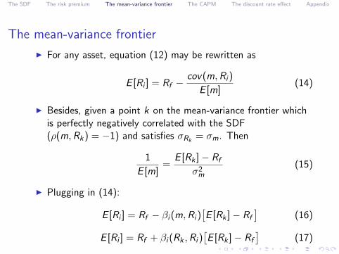
The mean-variance frontier

I For any asset, equation (12) may be rewritten as

E [Ri ] = Rf −cov(m,Ri )

E [m](14)

I Besides, given a point k on the mean-variance frontier whichis perfectly negatively correlated with the SDF(ρ(m,Rk) = −1) and satisfies σRk

= σm. Then

1

E [m]=

E [Rk ]− Rf

σ2m

(15)

I Plugging in (14):

E [Ri ] = Rf − βi (m,Ri )[E [Rk ]− Rf

](16)

E [Ri ] = Rf + βi (Rk ,Ri )[E [Rk ]− Rf

](17)


The CAPM

I The SDF involves consumption. Can we express the expectedreturns on any asset as a function of the expected returns onanother asset or portfolio of assets?

I This is the principle of the CAPM. It can be derived withquadratic utility, or normally distributed asset returns.

I In any of these two cases, the expected utility associated withany portfolio (a portfolio is a combination of assets) is fullydescribed by the mean and the variance of returns of thisportfolio.

I In this case, any investor will select a portfolio among a set ofmean-variance efficient portfolios.

I The set of mean-variance efficient portfolios is the set ofportfolios with the maximum expected return for a givenvariance of return – or equivalently the set of portfolios withthe minimum variance of returns for a given expected return.


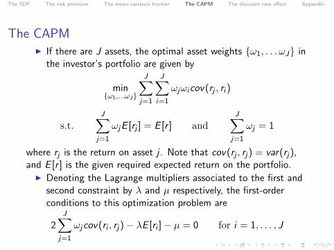
The CAPMI If there are J assets, the optimal asset weights {ω1, . . . ωJ} in

the investor’s portfolio are given by

min{ω1,...ωJ}

J∑j=1

J∑i=1

ωjωicov(rj , ri )

s.t.J∑

j=1

ωjE [rj ] = E [r ] andJ∑

j=1

ωj = 1

where rj is the return on asset j . Note that cov(rj , rj) = var(rj),and E [r ] is the given required expected return on the portfolio.

I Denoting the Lagrange multipliers associated to the first andsecond constraint by λ and µ respectively, the first-orderconditions to this optimization problem are

2J∑

j=1

ωjcov(ri , rj)− λE [ri ]− µ = 0 for i = 1, . . . , J


The CAPM

I Denote by rm =∑J

j=1 ωj rj the return on the market portfolio.Then

cov(rm, ri ) = cov( J∑

j=1

ωj rj , ri

)=

J∑j=1

cov(ωj rj , ri ) =J∑

j=1

ωjcov(rj , ri )

I Using this equation, we can rewrite the FOC as

2cov(rm, ri )− λE [ri ]− µ = 0 for i = 1, . . . , J (18)

I This equation should hold for the market portfolio:

2var [rm]− λE [rm]− µ = 0

I This equation should also hold for the riskfree asset:

−λrf − µ = 0


The CAPM

I Combining these two equations:

λ =2var [rm]

E [rm]− rfand µ = − 2var [rm]

E [rm]− rfrf

I Plugging these values of λ and µ in (18),

2cov(rm, ri )−2var [rm]

E [rm]− rfE [ri ] +

2var [rm]

E [rm]− rfrf = 0

Or

E [ri ]− rf =cov(ri , rm)

var [rm]

[E [rm]− rf

]


The CAPM

I We define

βi ≡cov(ri , rm)

var [rm]

I The beta of any asset measures its contribution to theriskiness of the market portfolio. Because of our assumptions,the riskiness is measured by the variance of returns.

I The expected excess return on any asset i is

E [ri ]− rf = βi

[E [rm]− rf

]I The right-hand-side of this equation is the risk premium.

With the CAPM, the risk premium is given by the quantity ofrisk in asset i , as measured with βi , multiplied by the price ofrisk, as measured by the expected excess return on the marketportfolio of risky assets.


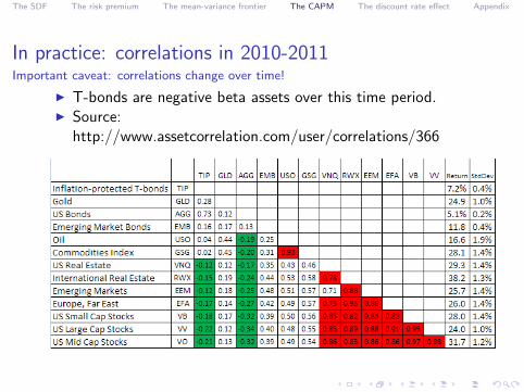
In practice: correlations in 2010-2011Important caveat: correlations change over time!

I T-bonds are negative beta assets over this time period.I Source:

http://www.assetcorrelation.com/user/correlations/366


The discount rate effect and the payoff effectWith log utility

I The wealth portfolio is a claim to all future consumption.Intuitively, if one owns all (respectively 1%) of the assets of alltypes in the economy, he has a claim to 100% (resp. 1%) ofall future consumption.

I The price of the wealth portfolio is

pMt = Et

[δu′(ct+1)

u′(ct)ct+1

]I With log utility (u(c) = ln(c)):

pMt = δct


The discount rate effect and the payoff effect

I Strangely, the portfolio price pMt does not depend on future

consumption.

I This is because two effects exactly offset each other with logutility. On the one hand, higher future consumption raises pM

t

(direct payoff effect). On the other hand, higher futureconsumption diminishes the SDF, which decreases pM

t

(indirect discounting effect).

I Importantly, this only holds for the wealth portfolio. Thiswould not be verified for individual assets: any news of higherfuture payoff would have a negligible effect on the SDF, sothat the payoff effect would be dominant.

I This effect must be kept in mind when there are news thatthe economy is becoming more productive (think about thelate 1990s). Should this raise asset prices? Not necessarily!


I Acknowledgements: Some sources for this series of slidesinclude:

I The slides of Martin Boyer, for the same course at HECMontreal.

I Asset Pricing, by John H. Cochrane.I Finance and the Economics of Uncertainty, by Gabrielle

Demange and Guy Laroque.I The Economics of Risk and Time, by Christian Gollier.


The CAPMAs derived with CRRA utility

I The SDF involves consumption. Can we express the expectedreturns of any asset as a function of the expected returns ofanother asset or portfolio of assets?

I This is the principle of the CAPM. It can be derived withquadratic utility or normally distributed returns.

I Here, we will derive it with CRRA utility, which is a commonlyused utility function in finance, and we won’t assume anythingon the distribution of returns. However, in discrete time, wewill need to work with approximations.

I The market portfolio includes all existing assets in theeconomy (stocks, bonds, real estate, commodities, etc.).Cochrane talks about a wealth portfolio which is a claim to allfuture consumption.



CAPM with consumption

I Denote by RMt+1 the return on the wealth portfolio.

I For agents with infinite horizons, ct+1

ct= Wt+1

Wt= RM

t+1.

I It follows that m = δ(

ct+1

ct

)−γ= δ(RM

t+1)−γ .

I Use a first order Taylor expansion to rewrite this term as

δ(RM)−γ ≈ δ(RM)−γ + δ(−γ)(RM)−γ−1(RM − RM)



I Equation (14) rewrites as

E [Ri ]− Rf = −cov(m,Ri )

E [m]

E [Ri ]− Rf = −cov(−δγ(RM)−γ−1(RM − RM),Ri )

E [m]

I For small time intervals, E [m] = R−1f ≈ 1 and δRM

−γ−1 ≈ 1

E [Ri ]− Rf = γcov(RM ,Ri ) = γcov(RM ,Ri )

var(RM)var(RM)

E [Ri ]− Rf = γβ(Ri ,RM)var(RM) (19)



I Setting i = M in (19) gives:

γvar(RM) = E [RM ]− Rf

I Substituting in (19):

E [Ri ]− Rf = βi

[E [RM ]− Rf

]I Remember that we used approximations to reach this result.


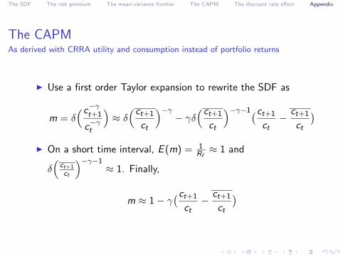
The CAPMAs derived with CRRA utility and consumption instead of portfolio returns

I Use a first order Taylor expansion to rewrite the SDF as

m = δ(c−γt+1

c−γt

)≈ δ(ct+1

ct

)−γ− γδ

(ct+1

ct

)−γ−1(ct+1

ct− ct+1

ct

)I On a short time interval, E (m) = 1

Rf≈ 1 and

δ(

ct+1

ct

)−γ−1≈ 1. Finally,

m ≈ 1− γ(ct+1

ct− ct+1

ct

)


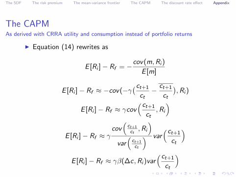
The CAPMAs derived with CRRA utility and consumption instead of portfolio returns

I Equation (14) rewrites as

E [Ri ]− Rf = −cov(m,Ri )

E [m]

E [Ri ]− Rf ≈ −cov(−γ(ct+1

ct− ct+1

ct

),Ri )

E [Ri ]− Rf ≈ γcov(ct+1

ct,Ri

)

E [Ri ]− Rf ≈ γcov(

ct+1

ct,Ri

)var(

ct+1

ct

) var(ct+1

ct

)E [Ri ]− Rf ≈ γβ(∆c,Ri )var

(ct+1

ct

)


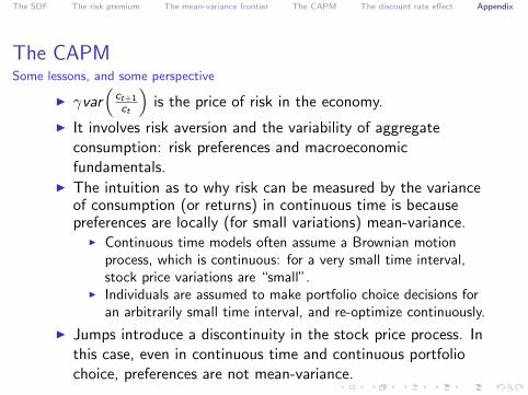
The CAPMSome lessons, and some perspective

I γvar(

ct+1

ct

)is the price of risk in the economy.

I It involves risk aversion and the variability of aggregateconsumption: risk preferences and macroeconomicfundamentals.

I The intuition as to why risk can be measured by the varianceof consumption (or returns) in continuous time is becausepreferences are locally (for small variations) mean-variance.

I Continuous time models often assume a Brownian motionprocess, which is continuous: for a very small time interval,stock price variations are “small”.

I Individuals are assumed to make portfolio choice decisions foran arbitrarily small time interval, and re-optimize continuously.

I Jumps introduce a discontinuity in the stock price process. Inthis case, even in continuous time and continuous portfoliochoice, preferences are not mean-variance.


More on the wealth portfolio

I With log utility, the price of the wealth portfolio with aninfinity of future periods (instead of one) is

pMt = Et

[ ∞∑τ=1

δτu′(ct+τ )

u′(ct)ct+τ

]= Et

[ ∞∑τ=1

δτct

ct+τct+τ

]= ct

δ

1− δ

I The return on the wealth portfolio is

RMt+1 ≡

pMt+1 + ct+1

pMt

=δ

1−δ + 1δ

1−δ

ct+1

ct

=1

δ

ct+1

ct=

(δu′(ct+1)

u′(ct)

)−1

= m−1t+1

The stochastic discount factor and the CAPM

Documents

Transcript of The stochastic discount factor and the CAPM