The Sports Labor Market – Part 2ECONOMICS OF SPORTS (ECON 325)

BEN VAN KAMMEN, PHD

IntroductionPlayer salaries primarily reflect expected future marginal revenue product.◦ A fraction of it, depending on the player’s bargaining position and reservation options.

As with any job, one’s productivity is not the only thing he gets paid for. Examples (not necessarily from sports):◦ Taking risks, e.g.,

◦ Of bodily injury or death [Garen (1988), and see “Related articles” on Google Scholar], or◦ Of unemployment [Abowd & Ashenfelter (1981)].

◦ Unpleasant working conditions, e.g.,◦ Physically [Duncan & Holmlund (1983)], ◦ Intellectually [Stern (2004)], or◦ Temporally [Golden (2001)].

◦ Foregoing valuable fringe benefits like health insurance [Royalty (2008)].

It would be unsurprising if athletes accept job amenities (endure disamenities) from clubs in lieu of higher (lower) salaries, too.

Introduction, continuedThinking about the club side of bargaining: wouldn’t players have “amenities” and “disamenities” too?◦ “Man of the Year” award winners versus, say, Aaron Hernandez, holding talent constant.◦ Paying athletes for good behavior/professionalism/character et al. probably socially valuable to the

league.

What about “amenities” that aren’t socially valuable?◦ Racial or ethnic discrimination: owners pay more to staff roster with players of the preferred race.◦ Again, independent of talent.

This lecture focuses on paying (getting paid) for non-productive traits.◦ When it’s (characteristics of) the club, it’s called a compensating wage differential, and it’s usually okay.◦ When it’s the player, it’s usually not okay to discriminate . . . but it’s complicated.

Compensating differentialsThere are numerous (dis)amenities that players may consider when choosing a salary offer.◦ Easiest to consider an unrestricted free agent, comparing all clubs.

Here we consider 2 transparent examples:◦ Income tax differences across the states where clubs are located, Kopkin (2012), and◦ Long term contracts (predictable, less uncertainty about salary over time), Krautmann & Oppenheimer

(2002), Link & Yosifov (2012).

Compensating differentials, theoryPlayers (“workers”) get utility from Income and fringe benefits.

You can illustrate how they are willing to trade off these goods using an indifference curve map.◦ Each indifference curve shows a set of bundles that makes the player equally “happy” (equal utility).

They slope down because you have to give them more of one good to make up for taking away units of the other good.◦ They’re steeper, the more the player likes income vis-à-vis benefits.

They are convex (bowed toward the origin) because the goods have diminishing marginal utility.

Further from the origin means a higher utility level.

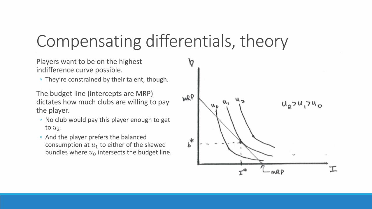
Compensating differentials, theoryPlayers want to be on the highest indifference curve possible.◦ They’re constrained by their talent, though.

The budget line (intercepts are MRP) dictates how much clubs are willing to pay the player.◦ No club would pay this player enough to get

to 𝑢𝑢2.◦ And the player prefers the balanced

consumption at 𝑢𝑢1 to either of the skewed bundles where 𝑢𝑢0 intersects the budget line.

Compensating differentials, theoryA player with different preferences would not choose the same (𝐼𝐼∗,𝑏𝑏∗) combination.

Drawing 2 tangencies on the same budget line illustrates how 2 players with the same talent (MRP) are faced with a trade-off of more benefits and less salary.

Compensating differentials, theory concludedContrast the trade-off, downward along the budget line, with the effect of a larger budget, i.e., being a better player.

When attempting to measure the trade-off in observed data, it’s important to compare players that are on the same budget (A to B).◦ I.e., control for differences in the height

(MRP).

Otherwise you’ll measure a positive effect of benefits on income (A to C).◦ Because when your MRP is higher, you can

“afford” more of both!

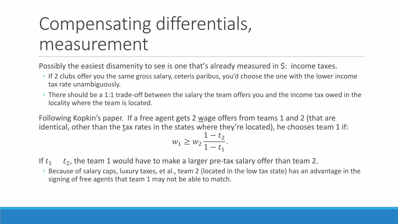
Compensating differentials, measurementPossibly the easiest disamenity to see is one that’s already measured in $: income taxes.◦ If 2 clubs offer you the same gross salary, ceteris paribus, you’d choose the one with the lower income

tax rate unambiguously.◦ There should be a 1:1 trade-off between the salary the team offers you and the income tax owed in the

locality where the team is located.

Following Kopkin’s paper. If a free agent gets 2 wage offers from teams 1 and 2 (that are identical, other than the tax rates in the states where they’re located), he chooses team 1 if:

𝑤𝑤1 ≥ 𝑤𝑤21 − 𝑡𝑡21 − 𝑡𝑡1

.

If 𝑡𝑡1 > 𝑡𝑡2, the team 1 would have to make a larger pre-tax salary offer than team 2.◦ Because of salary caps, luxury taxes, et al., team 2 (located in the low tax state) has an advantage in the

signing of free agents that team 1 may not be able to match.

Kopkin’s paper, empirical analysisData: 744 NBA free agents that signed contracts between 2001-02 and 2007-08.

Method: Regression of variables indicative of the accepted salary offers on the income tax rates in the states in which the signing team is located,◦ Controlling for other characteristics of the team and city: sales and property tax rates, population,

employment, and avg. income of the city, crime rate and student-teacher ratio in the city’s schools, the team’s room under the salary cap that season, and the team’s record the previous season.

Dependent variables (“𝑦𝑦𝑖𝑖𝑖𝑖”): skill level of signed player i, and salary of signed player i (going to team j in both cases).◦ Tax rate is hypothesized to decrease the average skill level of free agents signed by team j because it’s

harder to win the bidding wars, and◦ Tax rate is hypothesized to increase free agent salaries for team j because if you do win you had to pay

more than the rival club was offering.◦ “Skill” measured by performing a 3rd regression of salary on performance stats to assign a market value

to a player’s performance.

Kopkin’s paper, resultsFrom pp. 586-591.

1 percentage point decrease in the (marginal) income tax rate increases the skill level of the average free agent signed by the NBA team by about [0.08 to 0.09] standard deviations.◦ In tangible terms, considering the typical number of free agent signings per season, this additional skill

translates into about 4 wins per season on average.◦ Or about 2.4 playoff wins per season on average.◦ Indiana is doing well relative to the Central Division, but losing out on free agents to Miami, Atlanta, all

of Texas, and Seattle.

The tax rates are evidently not “capitalized” into salaries, since the effect of tax rate on salaries of signed free agents is insignificantly different from zero (pp. 593-594).

Teams “pay” with lower quality, rather than higher salaries.

Long term contracts and risk aversion, backgroundPlayers can negotiate over the length of their contracts, with 2 stylized options:

1. Strike a bargain each season, salary somewhere between the reservation and the expected Marginal Revenue Product the next season.

2. Striking a bargain over multiple future seasons, salaries somewhere between the reservation and the expected MRP, summed over the length of the contract.

Players know there is a risk of their MRP decreasing in the future (injury, decline in skill).◦ Possibly to the point where they are out of sports and making their reservation wage: “HS phys. ed.

teacher.”

If they are risk averse, they are willing to trade less money in the high MRP state (“coming off a strong ‘walk’ year”) for more money in the low MRP state (“coming off a down ‘walk’ year”).◦ If choosing option #2 above, the player is willing to accept an additional discount (less salary) on his

expected MRP, in exchange for more certainty over the length of the contract.

Risk aversion, formallyAssume there are 2 (equally likely, 𝑝𝑝 = 1 − 𝑝𝑝 = 0.5) outcomes for next year’s negotiations:◦ Player’s 𝐸𝐸(𝑀𝑀𝑀𝑀𝑀𝑀|𝑠𝑠𝑡𝑡𝑠𝑠𝑠𝑠𝑠𝑠𝑠𝑠) = 𝑠𝑠0 (coming off good year) and◦ Players 𝐸𝐸 𝑀𝑀𝑀𝑀𝑀𝑀|𝑤𝑤𝑤𝑤𝑤𝑤𝑤𝑤 = 𝑠𝑠1 = 𝑠𝑠𝑤𝑤𝑠𝑠𝑤𝑤𝑠𝑠𝑟𝑟𝑤𝑤𝑡𝑡𝑟𝑟𝑠𝑠𝑠𝑠 𝑤𝑤𝑤𝑤𝑠𝑠𝑤𝑤 < 𝑠𝑠0 (coming off bad year).

The player’s utility function is: 𝑈𝑈 = 2𝑤𝑤00.5 + 2𝑤𝑤10.5, where w is his salary in the strong (0) and weak (1) states.

Without a long term contract, his expected utility is: 𝐸𝐸(𝑈𝑈) = 𝑠𝑠00.5 + 𝑠𝑠10.5.

Risk aversion is the idea that expected utility is less than the utility if you gave him his expected MRP with certainty.

𝐸𝐸 𝑈𝑈 < 𝑈𝑈𝑠𝑠0 + 𝑠𝑠1

2⇔ 𝑠𝑠00.5 + 𝑠𝑠10.5 < 2

𝑠𝑠0 + 𝑠𝑠12

0.5.

Showing this is left as an exercise, but algebraically it is true and these preferences are risk averse.

The compensating differential for riskIt’s called willingness to pay for insurance.

You can show that there is a multi-year salary, �̅�𝑠 < 𝑠𝑠0+𝑠𝑠12

, that gives the player equal utility to that of the 1-year contracts.◦ The difference, 𝑠𝑠0+𝑠𝑠1

2− �̅�𝑠, is the player’s compensating differential.

◦ What he’s willing to pay to insure himself against the risk of lower future salary.◦ �̅�𝑠 is called his certainty equivalence in the jargon.

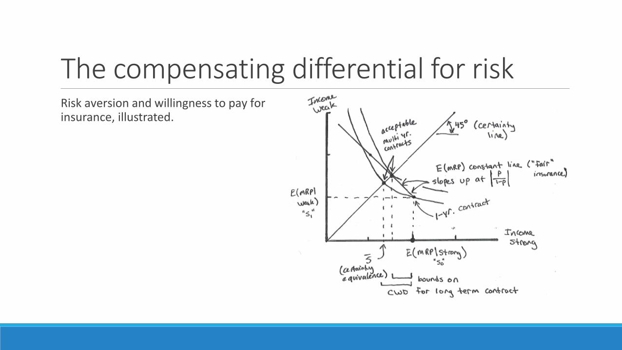
The compensating differential for riskRisk aversion and willingness to pay for insurance, illustrated.

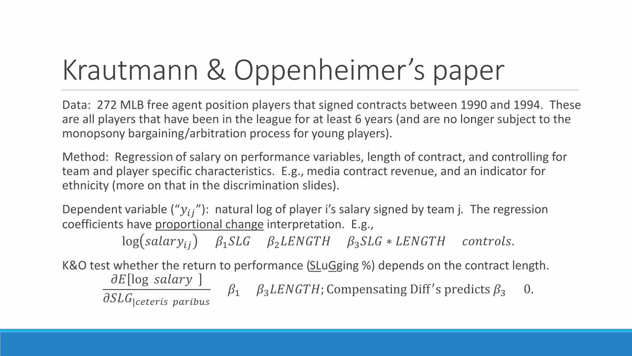
Krautmann & Oppenheimer’s paperData: 272 MLB free agent position players that signed contracts between 1990 and 1994. These are all players that have been in the league for at least 6 years (and are no longer subject to the monopsony bargaining/arbitration process for young players).

Method: Regression of salary on performance variables, length of contract, and controlling for team and player specific characteristics. E.g., media contract revenue, and an indicator for ethnicity (more on that in the discrimination slides).

Dependent variable (“𝑦𝑦𝑖𝑖𝑖𝑖”): natural log of player i’s salary signed by team j. The regression coefficients have proportional change interpretation. E.g.,

log 𝑠𝑠𝑤𝑤𝑠𝑠𝑤𝑤𝑠𝑠𝑦𝑦𝑖𝑖𝑖𝑖 = 𝛽𝛽1𝑆𝑆𝑆𝑆𝑆𝑆 + 𝛽𝛽2𝑆𝑆𝐸𝐸𝐿𝐿𝑆𝑆𝐿𝐿𝐿𝐿 + 𝛽𝛽3𝑆𝑆𝑆𝑆𝑆𝑆 ∗ 𝑆𝑆𝐸𝐸𝐿𝐿𝑆𝑆𝐿𝐿𝐿𝐿 + 𝑐𝑐𝑠𝑠𝑠𝑠𝑡𝑡𝑠𝑠𝑠𝑠𝑠𝑠𝑠𝑠.

K&O test whether the return to performance (SLuGging %) depends on the contract length.𝜕𝜕𝐸𝐸 log(𝑠𝑠𝑤𝑤𝑠𝑠𝑤𝑤𝑠𝑠𝑦𝑦)𝜕𝜕𝑆𝑆𝑆𝑆𝑆𝑆|𝑐𝑐𝑐𝑐𝑐𝑐𝑐𝑐𝑐𝑐𝑖𝑖𝑠𝑠 𝑝𝑝𝑝𝑝𝑐𝑐𝑖𝑖𝑝𝑝𝑝𝑝𝑠𝑠

= 𝛽𝛽1 + 𝛽𝛽3𝑆𝑆𝐸𝐸𝐿𝐿𝑆𝑆𝐿𝐿𝐿𝐿; Compensating Diff ′s predicts 𝛽𝛽3 < 0.

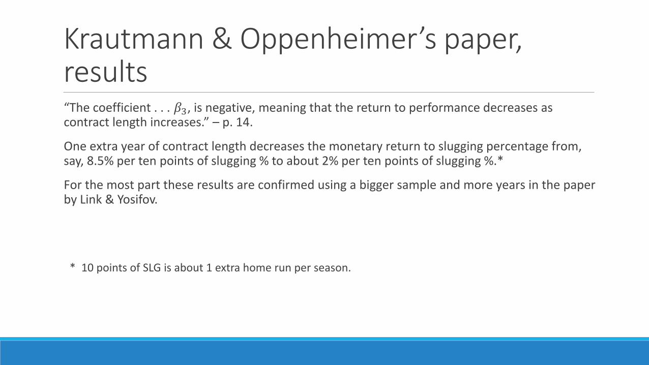
Krautmann & Oppenheimer’s paper, results“The coefficient . . . 𝛽𝛽3, is negative, meaning that the return to performance decreases as contract length increases.” – p. 14.

One extra year of contract length decreases the monetary return to slugging percentage from, say, 8.5% per ten points of slugging % to about 2% per ten points of slugging %.*

For the most part these results are confirmed using a bigger sample and more years in the paper by Link & Yosifov.

* 10 points of SLG is about 1 extra home run per season.

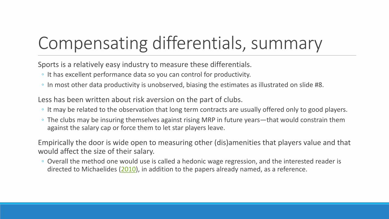
Compensating differentials, summarySports is a relatively easy industry to measure these differentials.◦ It has excellent performance data so you can control for productivity.◦ In most other data productivity is unobserved, biasing the estimates as illustrated on slide #8.

Less has been written about risk aversion on the part of clubs.◦ It may be related to the observation that long term contracts are usually offered only to good players.◦ The clubs may be insuring themselves against rising MRP in future years—that would constrain them

against the salary cap or force them to let star players leave.

Empirically the door is wide open to measuring other (dis)amenities that players value and that would affect the size of their salary.◦ Overall the method one would use is called a hedonic wage regression, and the interested reader is

directed to Michaelides (2010), in addition to the papers already named, as a reference.

DiscriminationSalary differences among players is okay as long as those differences are based on skill/talent/productivity.

If there are differences in salary across racial or ethnic groups, holding talent constant, one or more groups is being treated unfairly (discriminated against).◦ Corollary: a club that doesn’t discriminate could outbid other clubs for stars from the less-preferred

group and afford a more talented roster.

For discrimination to persist, it must originate with the preferences of the fans or other players.◦ If a club can attract more fans or better players by employing the favored group, competition will not

punish them for responding by discriminating.

Salary differences as a testReally famous labor economist Lawrence Kahn wrote several papers about racial salary differences in sports that are like the Jordan-Pippen-Jackson-non-Rodman Bulls of this literature.◦ And happened more or less contemporaneously.

About the NBA (with Peter Sherer, 1988), a survey of the existing literature (1991), and about the NFL (1992).

Salary differences are not the only way to infer discrimination, e.g.,◦ Likelihood of being hired into the league (would need data on the amateurs for comparison, though),◦ Segregation by position,◦ Customer discrimination, e.g., in jersey sales or baseball cards [Nardinelli & Simon (1990)],◦ Recording conversations with owners.

But salary differences are the focus here due to the prominence in the literature and the similarity in estimation method to compensating differentials.

Kahn and Sherer’s NBA paperTest whether:◦ the MRP depends on Race (customer/fan discrimination), ◦ the share (a) of the MRP the player gets as salary depends on Race (team(mate) discrimination), or◦ both.

Controlling for team characteristics, e.g., record the year prior, income and racial composition of the city where located.

But you don’t observe MRP, just estimate it based on performance variables, so both types of discrimination lumped into the same coefficient on Race:

log 𝑠𝑠𝑤𝑤𝑠𝑠𝑤𝑤𝑠𝑠𝑦𝑦𝑖𝑖𝑖𝑖 = 𝛽𝛽𝑀𝑀𝑤𝑤𝑠𝑠𝛽𝛽𝑠𝑠𝑠𝑠𝛽𝛽𝑤𝑤𝑠𝑠𝑐𝑐𝑤𝑤𝑖𝑖 + 𝛿𝛿𝑀𝑀 + 𝑐𝑐𝑠𝑠𝑠𝑠𝑡𝑡𝑠𝑠𝑠𝑠𝑠𝑠𝑠𝑠.

𝑀𝑀 = �1 for white players,0 for black players.

Kahn and Sherer’s NBA paper, continuedIs 𝛿𝛿 > 0? Estimate the salary regression to see if, conditional on performance, race affects salary.◦ Using 226 NBA players in 1985-1986 season.

Interesting offshoots: ◦ Does (league entry) draft order depend on race, conditional on college performance?◦ To get at the distinction between fan and team discrimination, does home attendance (controlling for

other determinants like win % and ticket price) depend on the racial composition of the team’s roster?◦ Using team-level observations from 1981-1986.◦ Operationalized as the % of the roster that is white.

Kahn and Sherer’s resultsWhite NBA players earn roughly a 20% salary premium compared to equal performing black players.◦ Premium may go up with seniority in the league,◦ The premium is not bigger in cities with more white people.

White players, college performance being equal, are drafted later than black players with similar résumés, but the difference isn’t statistically significant.

There is probably a small positive effect on attendance caused by having more white players.◦ Again, effect is independent of the racial composition of the city in which the team is located.

Since the sample (mid 1980s) is from a time when player free agency has been around awhile, the persistence of salary differences in an (internally) competitive labor market is unlikely.◦ It’s not a smoking gun but the authors states that his results support customer discrimination.

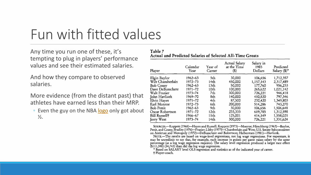
Fun with fitted valuesAny time you run one of these, it’s tempting to plug in players’ performance values and see their estimated salaries.

And how they compare to observed salaries.

More evidence (from the distant past) that athletes have earned less than their MRP.◦ Even the guy on the NBA logo only got about

½.

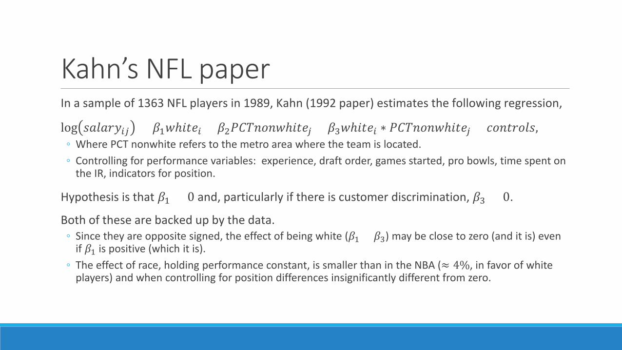
Kahn’s NFL paperIn a sample of 1363 NFL players in 1989, Kahn (1992 paper) estimates the following regression,

log 𝑠𝑠𝑤𝑤𝑠𝑠𝑤𝑤𝑠𝑠𝑦𝑦𝑖𝑖𝑖𝑖 = 𝛽𝛽1𝑤𝑤𝑤𝑟𝑟𝑡𝑡𝑤𝑤𝑖𝑖 + 𝛽𝛽2𝑀𝑀𝑃𝑃𝐿𝐿𝑠𝑠𝑠𝑠𝑠𝑠𝑤𝑤𝑤𝑟𝑟𝑡𝑡𝑤𝑤𝑖𝑖 + 𝛽𝛽3𝑤𝑤𝑤𝑟𝑟𝑡𝑡𝑤𝑤𝑖𝑖 ∗ 𝑀𝑀𝑃𝑃𝐿𝐿𝑠𝑠𝑠𝑠𝑠𝑠𝑤𝑤𝑤𝑟𝑟𝑡𝑡𝑤𝑤𝑖𝑖 + 𝑐𝑐𝑠𝑠𝑠𝑠𝑡𝑡𝑠𝑠𝑠𝑠𝑠𝑠𝑠𝑠,◦ Where PCT nonwhite refers to the metro area where the team is located.◦ Controlling for performance variables: experience, draft order, games started, pro bowls, time spent on

the IR, indicators for position.

Hypothesis is that 𝛽𝛽1 > 0 and, particularly if there is customer discrimination, 𝛽𝛽3 < 0.

Both of these are backed up by the data.◦ Since they are opposite signed, the effect of being white (𝛽𝛽1 + 𝛽𝛽3) may be close to zero (and it is) even

if 𝛽𝛽1 is positive (which it is).◦ The effect of race, holding performance constant, is smaller than in the NBA (≈ 4%, in favor of white

players) and when controlling for position differences insignificantly different from zero.

Kahn’s NFL paper, conclusionThere may be a modest salary premium for white players in the NFL, but the most striking result is the preference of fans to see players of their race.◦ This goes both ways: whiter cities like whiter football teams and less white cities like less white football

teams.

The positional segregation in the NFL is not examined much in the paper, but given the importance of the position controls, and the uneven distribution of white players (QB, OL, LB, special teams), this warrants more attention.

Subsequent literature, similar methodsHamilton (1997): update on Kahn & Sherer about the 1990s . . . white salary premium persists, only at the top end of the talent distribution. “Fans favor white star NBA players.”

Bodvarsson & Brastow (1998): once you control for consistency in performance, the significance of the race coefficient, estimated on NBA data, goes away, i.e., no evidence of discrimination.◦ Dey (1997) doesn’t find one either.◦ Eschker, Perez & Siegler (2004): the winner’s curse applied to Int’l NBA players in the mid 90s.

Jones, Nadeau & Walsh (1999): very limited evidence of discrimination by nationality in NHL.

Gius & Johnson (2000): reverse (10% in favor of black players) discrimination in 1995 NFL data.◦ Keefer (2013): at the linebacker position, black players are discriminated against, throughout the

distribution (across marginal to stars).

This is just a sample of the energy that has been expended on this question.

Szymanski’s (2000) paperThe “market test” for discrimination doesn’t assume you can control for skill differences in a regression.

Instead, all you have to do is see whether racial composition of clubs affects their on-field competitiveness.◦ If you’re not discriminating, your success should just depend on your payroll,◦ Not the skin color of the players on that payroll.◦ It should not be possible to win more games by swapping white players for black (or vice versa).

Looks at 39 English soccer league clubs for 16 seasons (1978-1993), 624 observations.

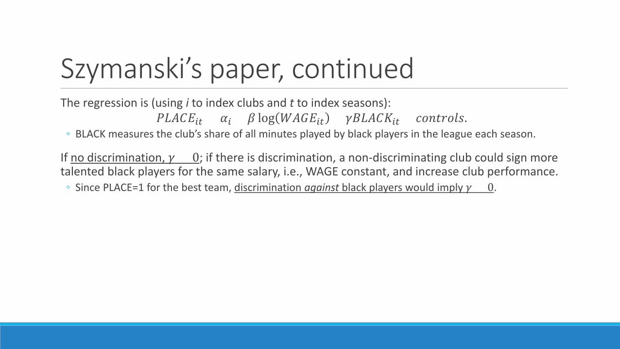
Szymanski’s paper, continuedThe regression is (using i to index clubs and t to index seasons):

𝑀𝑀𝑆𝑆𝑃𝑃𝑃𝑃𝐸𝐸𝑖𝑖𝑐𝑐 = 𝛼𝛼𝑖𝑖 + 𝛽𝛽 log 𝑊𝑊𝑃𝑃𝑆𝑆𝐸𝐸𝑖𝑖𝑐𝑐 + 𝛾𝛾𝛾𝛾𝑆𝑆𝑃𝑃𝑃𝑃𝐾𝐾𝑖𝑖𝑐𝑐 + 𝑐𝑐𝑠𝑠𝑠𝑠𝑡𝑡𝑠𝑠𝑠𝑠𝑠𝑠𝑠𝑠.◦ BLACK measures the club’s share of all minutes played by black players in the league each season.

If no discrimination, 𝛾𝛾 = 0; if there is discrimination, a non-discriminating club could sign more talented black players for the same salary, i.e., WAGE constant, and increase club performance.◦ Since PLACE=1 for the best team, discrimination against black players would imply 𝛾𝛾 < 0.

Szymanski’s resultsThe estimates of 𝛾𝛾 are negative. They are only statistically significant for the later part of the sample, 1986-1993, when there were more black players in the league.◦ Splitting the sample by the size of the market (as measured by stadium capacity), discrimination is only

detected among the largest clubs.

In practical terms, “. . . a club hiring no black players would have paid a 5 percent premium in terms of its total wage bill to maintain any given position in the league compared to a non-discriminating team (i.e., one that hired an average number of black players).” – p. 600.

To infer whether discrimination originates with fans or owners, Szymanski found that the prevalence of black players had neither an effect on attendance nor ticket revenues.◦ This suggests it is the owners that are discriminating.

The optimistic conclusion: as the league grows in popularity, professional investors will buy more of the clubs from the “hobby business[men]” that owned them at the time of publication.◦ They would be more apt to colorblind-ly maximize profit than a Donald Sterling-type.

“Market test” for NFL coaches(not John) Madden (2004 & 2011, with Matthew Ruther) studied the small number of black head coaches in the NFL using a similar method. ◦ If black NFL coaches collectively performed better than white head coaches, it would suggest that the

marginal black coach is better than the marginal white coach,◦ and that teams are hiring lower quality white coaches than black coaches (discriminating).

The 2004 paper looks at the period 1990-2002 and finds that black coaches were doing better, i.e., there weren’t enough marginal ones to bring down their group average.

The 2011 paper looks at the post-“Rooney Rule” period (2003-), after which interviewing at least one black coaching candidate was mandatory in the NFL.

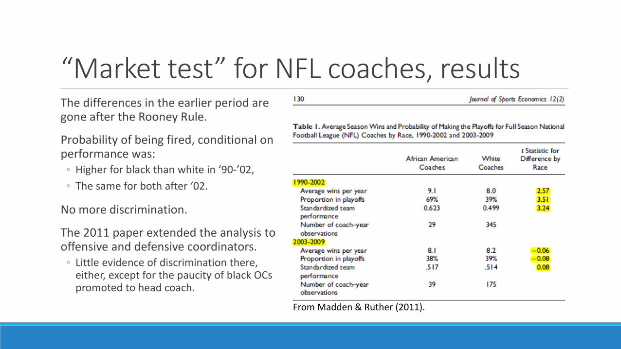
“Market test” for NFL coaches, resultsThe differences in the earlier period are gone after the Rooney Rule.

Probability of being fired, conditional on performance was:◦ Higher for black than white in ‘90-’02,◦ The same for both after ‘02.

No more discrimination.

The 2011 paper extended the analysis to offensive and defensive coordinators.◦ Little evidence of discrimination there,

either, except for the paucity of black OCs promoted to head coach.

From Madden & Ruther (2011).

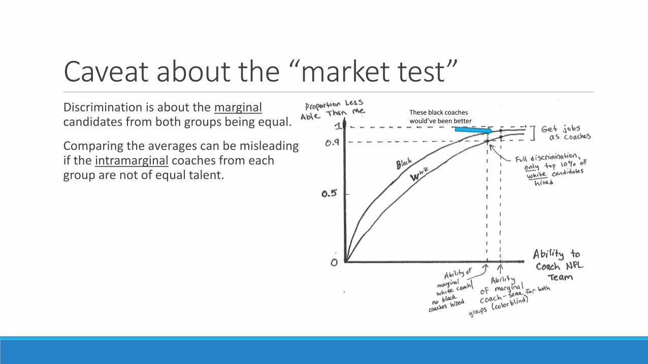
Caveat about the “market test”Discrimination is about the marginalcandidates from both groups being equal.

Comparing the averages can be misleading if the intramarginal coaches from each group are not of equal talent.

These black coaches would’ve been better

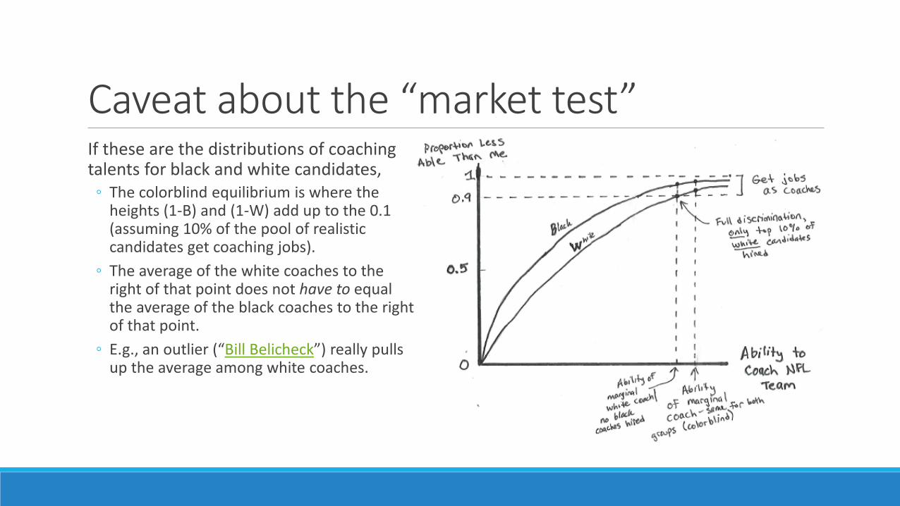
Caveat about the “market test”If these are the distributions of coaching talents for black and white candidates,◦ The colorblind equilibrium is where the

heights (1-B) and (1-W) add up to the 0.1 (assuming 10% of the pool of realistic candidates get coaching jobs).

◦ The average of the white coaches to the right of that point does not have to equal the average of the black coaches to the right of that point.

◦ E.g., an outlier (“Bill Belicheck”) really pulls up the average among white coaches.

ConclusionHopefully these examples illustrate the reasons that led Lawrence Kahn (2000) to call sports a “Labor Market Laboratory.”

The player salary regression is so versatile for testing theories about implicit transactions, e.g., of job amenities, and discrimination.◦ It’s such a good “laboratory” because of the wide availability of performance and salary data.

A Labor Economics class would attempt to generalize these observations to other professions where the data is less good (and salaries are generally lower), i.e., for “the rest of us.”◦ You usually need more advanced statistical methods (take “Econometrics”) to overcome the data

limitations, though.

Since so much has been written on the subject of the sports production function (of wins) and the comparison of players’ productivities (“sabermetrics”), the next lecture briefly indulges this interest by evaluating the usefulness of various performance measures.

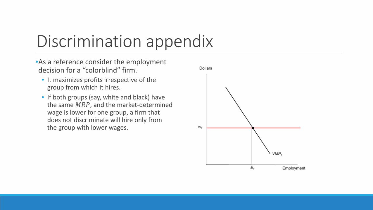
Discrimination appendix•As a reference consider the employment decision for a “colorblind” firm.• It maximizes profits irrespective of the

group from which it hires. • If both groups (say, white and black) have

the same 𝑀𝑀𝑀𝑀𝑀𝑀, and the market-determined wage is lower for one group, a firm that does not discriminate will hire only from the group with lower wages.

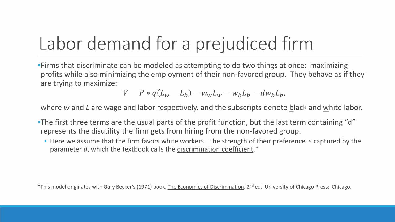
Labor demand for a prejudiced firm•Firms that discriminate can be modeled as attempting to do two things at once: maximizing profits while also minimizing the employment of their non-favored group. They behave as if they are trying to maximize:

𝑉𝑉 = 𝑀𝑀 ∗ 𝑞𝑞 𝑆𝑆𝑤𝑤 + 𝑆𝑆𝑝𝑝 − 𝑤𝑤𝑤𝑤𝑆𝑆𝑤𝑤 − 𝑤𝑤𝑝𝑝𝑆𝑆𝑝𝑝 − 𝑑𝑑𝑤𝑤𝑝𝑝𝑆𝑆𝑝𝑝,

where w and L are wage and labor respectively, and the subscripts denote black and white labor.

•The first three terms are the usual parts of the profit function, but the last term containing “d” represents the disutility the firm gets from hiring from the non-favored group.• Here we assume that the firm favors white workers. The strength of their preference is captured by the

parameter d, which the textbook calls the discrimination coefficient.*

*This model originates with Gary Becker’s (1971) book, The Economics of Discrimination, 2nd ed. University of Chicago Press: Chicago.

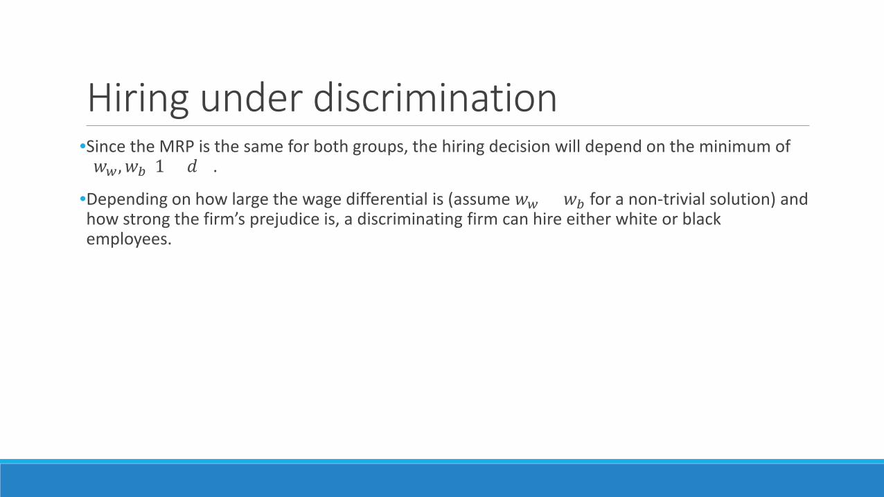
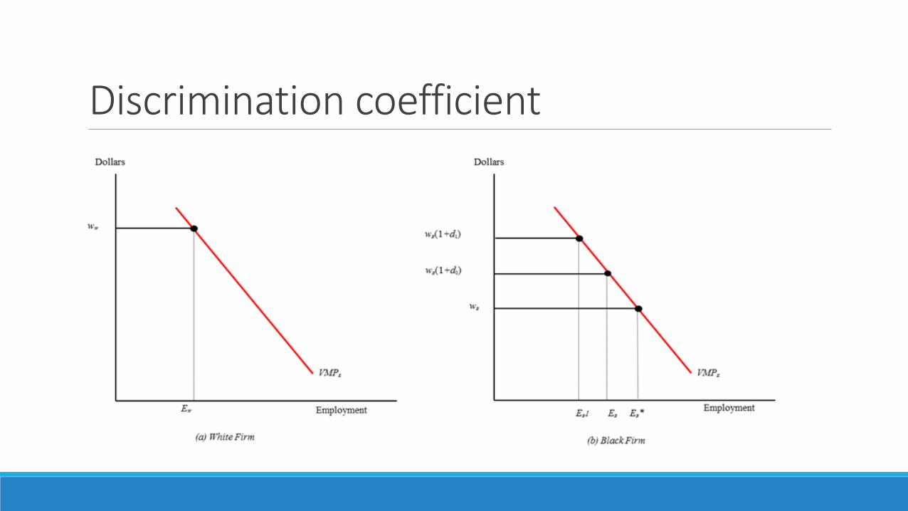
Hiring under discrimination•Since the MRP is the same for both groups, the hiring decision will depend on the minimum of {𝑤𝑤𝑤𝑤,𝑤𝑤𝑝𝑝(1 + 𝑑𝑑)}.

•Depending on how large the wage differential is (assume 𝑤𝑤𝑤𝑤 > 𝑤𝑤𝑝𝑝 for a non-trivial solution) and how strong the firm’s prejudice is, a discriminating firm can hire either white or black employees.

Discrimination coefficient

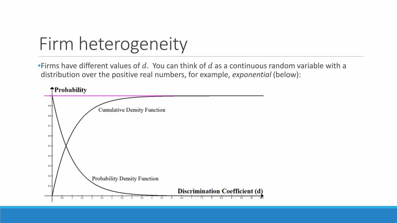
Firm heterogeneity•Firms have different values of 𝑑𝑑. You can think of 𝑑𝑑 as a continuous random variable with a distribution over the positive real numbers, for example, exponential (below):

Distribution of discrimination preferences

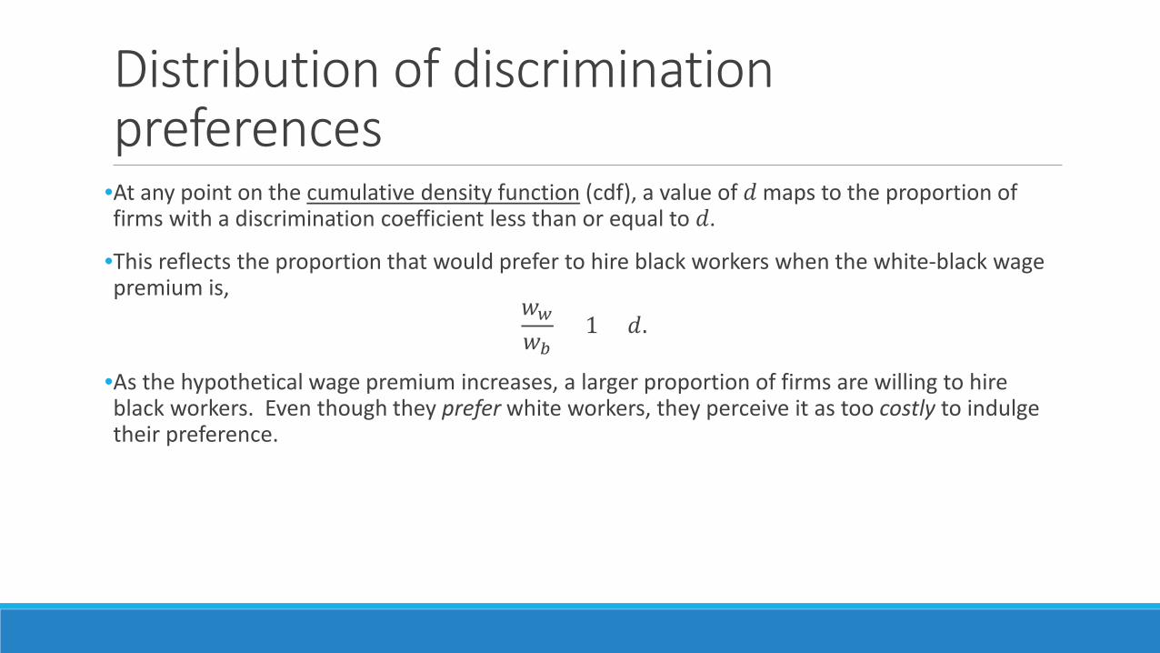
•At any point on the cumulative density function (cdf), a value of 𝑑𝑑 maps to the proportion of firms with a discrimination coefficient less than or equal to 𝑑𝑑.

•This reflects the proportion that would prefer to hire black workers when the white-black wage premium is,

𝑤𝑤𝑤𝑤𝑤𝑤𝑝𝑝

= 1 + 𝑑𝑑.

•As the hypothetical wage premium increases, a larger proportion of firms are willing to hire black workers. Even though they prefer white workers, they perceive it as too costly to indulge their preference.

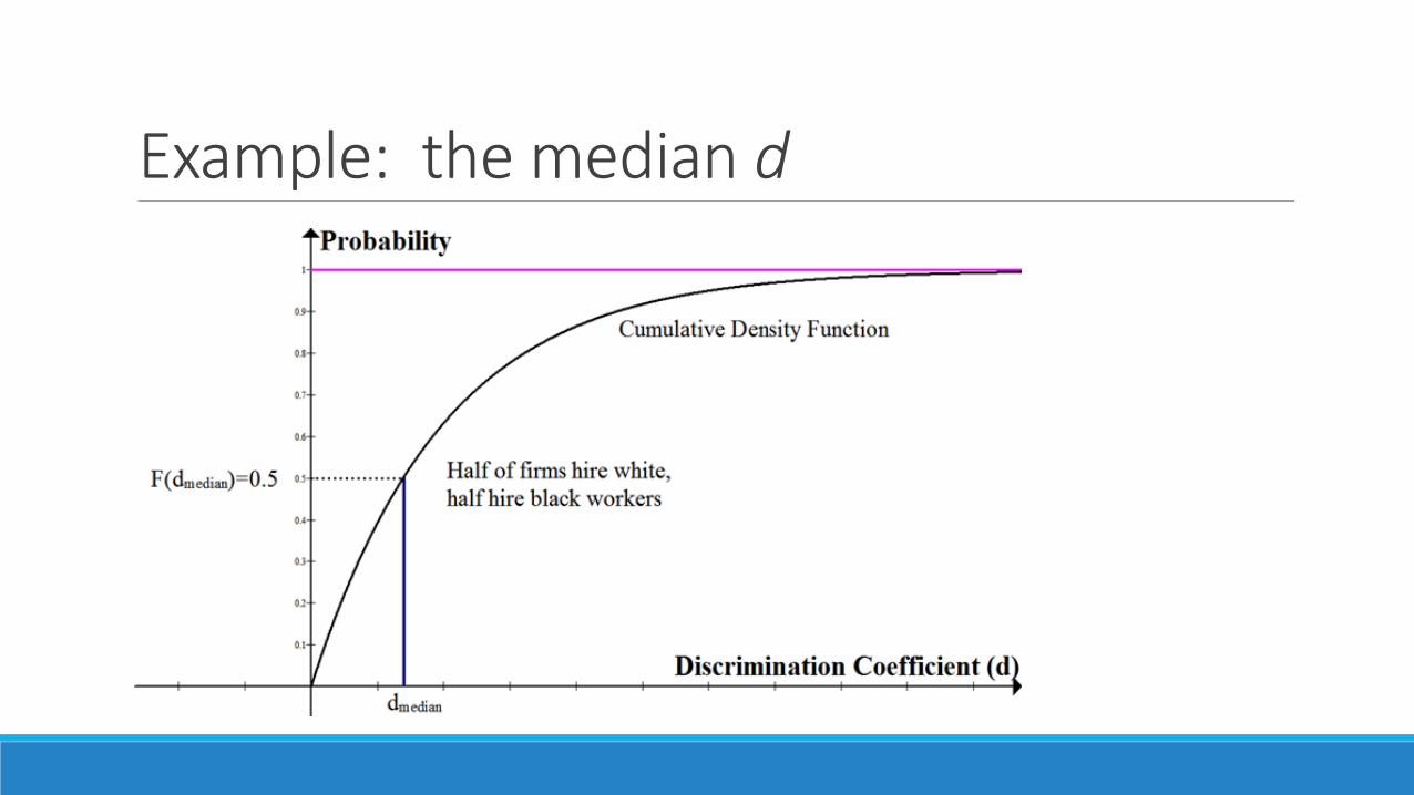
Example: the median d

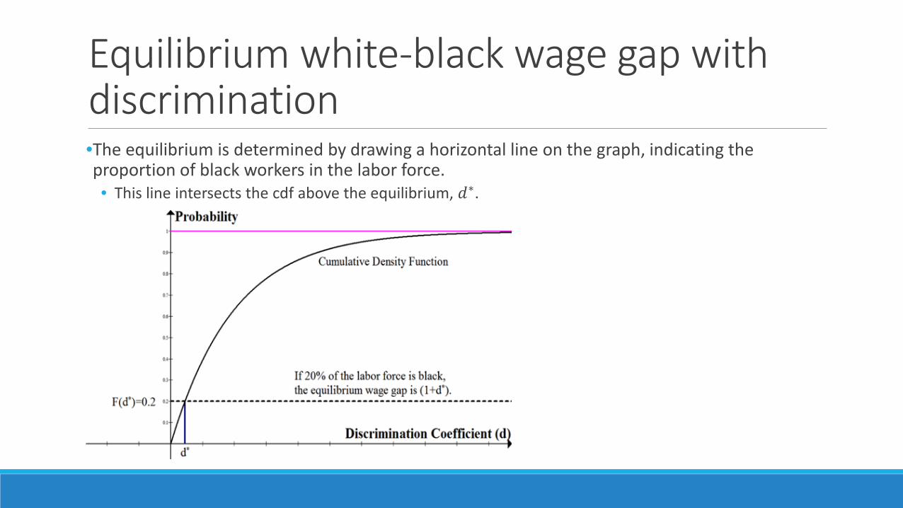
Equilibrium white-black wage gap with discrimination•The equilibrium is determined by drawing a horizontal line on the graph, indicating the proportion of black workers in the labor force.• This line intersects the cdf above the equilibrium, 𝑑𝑑∗.

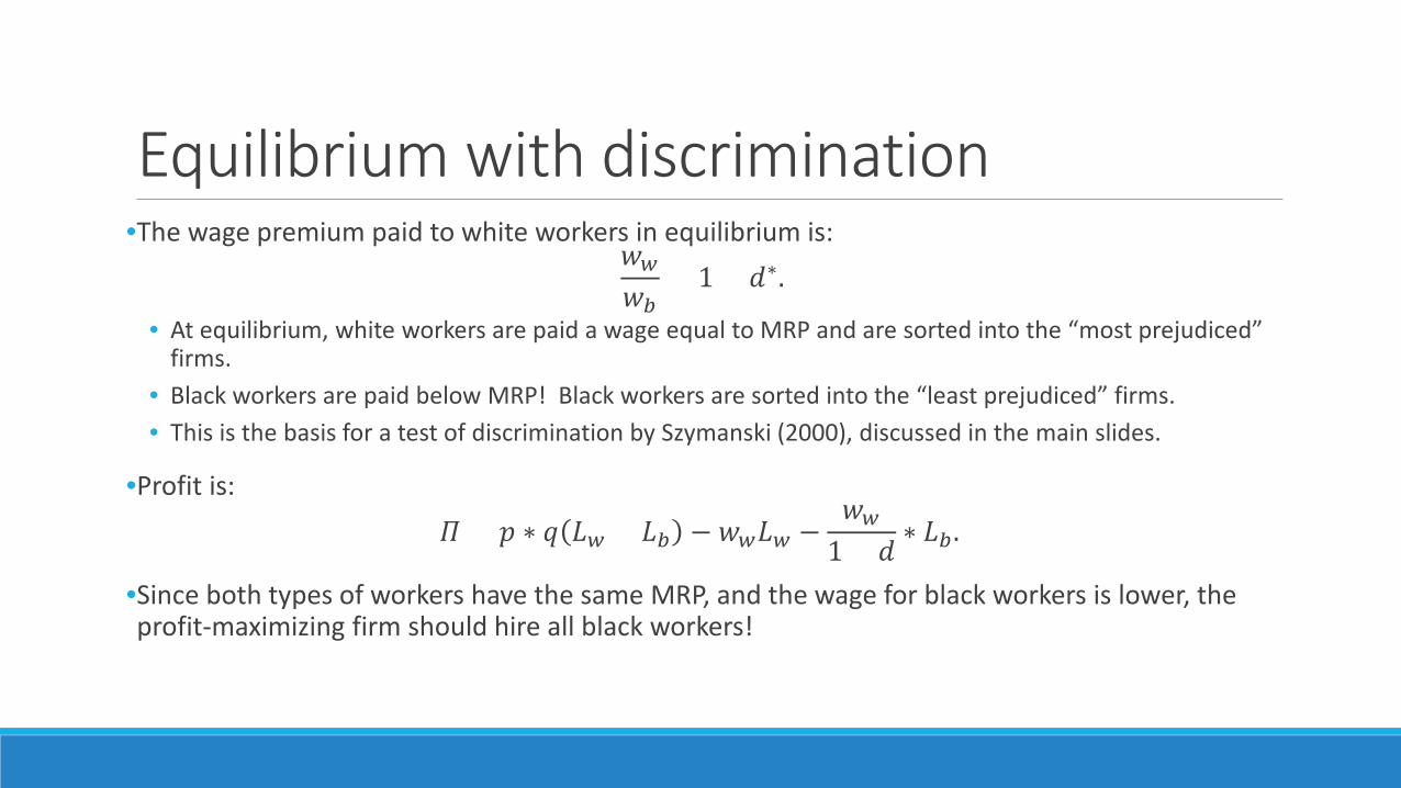
Equilibrium with discrimination•The wage premium paid to white workers in equilibrium is:

𝑤𝑤𝑤𝑤𝑤𝑤𝑝𝑝

= 1 + 𝑑𝑑∗.

• At equilibrium, white workers are paid a wage equal to MRP and are sorted into the “most prejudiced” firms.

• Black workers are paid below MRP! Black workers are sorted into the “least prejudiced” firms.• This is the basis for a test of discrimination by Szymanski (2000), discussed in the main slides.

•Profit is:𝛱𝛱 = 𝑝𝑝 ∗ 𝑞𝑞 𝑆𝑆𝑤𝑤 + 𝑆𝑆𝑝𝑝 − 𝑤𝑤𝑤𝑤𝑆𝑆𝑤𝑤 −

𝑤𝑤𝑤𝑤1 + 𝑑𝑑

∗ 𝑆𝑆𝑝𝑝.

•Since both types of workers have the same MRP, and the wage for black workers is lower, the profit-maximizing firm should hire all black workers!

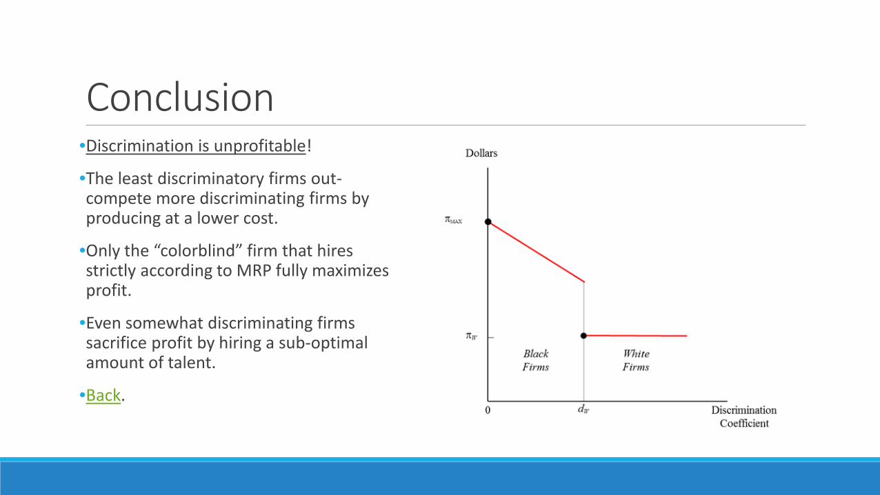
Conclusion•Discrimination is unprofitable!

•The least discriminatory firms out-compete more discriminating firms by producing at a lower cost.

•Only the “colorblind” firm that hires strictly according to MRP fully maximizes profit.

•Even somewhat discriminating firms sacrifice profit by hiring a sub-optimal amount of talent.

•Back.