DI

SC

US

SI

ON

P

AP

ER

S

ER

IE

S

Forschungsinstitut zur Zukunft der ArbeitInstitute for the Study of Labor

Labor Market Effects of Sports and Exercise:Evidence from Canadian Panel Data

IZA DP No. 7931

January 2014

Michael LechnerNazmi Sari

Labor Market Effects of Sports and Exercise:

Evidence from Canadian Panel Data

Michael Lechner SEW, University of St. Gallen,

CEPR, PSI, CESifo, IAB and IZA

Nazmi Sari University of Saskatchewan,

SPHERU and Health Quality Council, Saskatoon

Discussion Paper No. 7931 January 2014

IZA

P.O. Box 7240 53072 Bonn

Germany

Phone: +49-228-3894-0 Fax: +49-228-3894-180

E-mail: iza@iza.org

Any opinions expressed here are those of the author(s) and not those of IZA. Research published in this series may include views on policy, but the institute itself takes no institutional policy positions. The IZA research network is committed to the IZA Guiding Principles of Research Integrity. The Institute for the Study of Labor (IZA) in Bonn is a local and virtual international research center and a place of communication between science, politics and business. IZA is an independent nonprofit organization supported by Deutsche Post Foundation. The center is associated with the University of Bonn and offers a stimulating research environment through its international network, workshops and conferences, data service, project support, research visits and doctoral program. IZA engages in (i) original and internationally competitive research in all fields of labor economics, (ii) development of policy concepts, and (iii) dissemination of research results and concepts to the interested public. IZA Discussion Papers often represent preliminary work and are circulated to encourage discussion. Citation of such a paper should account for its provisional character. A revised version may be available directly from the author.

IZA Discussion Paper No. 7931 January 2014

ABSTRACT

Labor Market Effects of Sports and Exercise: Evidence from Canadian Panel Data*

Based on the Canadian National Population Health Survey we estimate the effects of individual sports and exercise on individual labor market outcomes. The data covers the period from 1994 to 2008. It is longitudinal and rich in life-style, health, and physical activity information. Exploiting these features of the data allows for a credible identification of the effects as well as for estimating dose-response relationships. Generally, we confirm previous findings of positive long-run income effects. However, an activity level above the current recommendation of the WHO for minimum physical activity is required to reap in the long-run benefits. JEL Classification: I12, I18, J24, L83, C21 Keywords: physical activity, Canadian National Population Health Survey, individual

sports participation, human capital, labor market, matching estimation Corresponding author: Michael Lechner Swiss Institute for Empirical Economic Research (SEW) University of St. Gallen Varnbüelstrasse 14 9000 St. Gallen Switzerland E-mail: Michael.Lechner@unisg.ch

* All computations have been performed in the Statistics Canada Research Data Center at the University of Saskatchewan in Saskatoon. We thank the Data Center and Statistics Canada for their support. All computations were implemented with our own programs using Gauss 11 installed in the Data Center. A previous version of the paper was presented at IZA, Bonn, ZEW, Mannheim, and the Alpine Labour Seminar, Laax. We thank participants for helpful comments and suggestions. The usual disclaimer applies.

1

1 Introduction

Do the positive health effects of physical activity1 translate into higher productivity of

the labor force and thus higher earnings? Although potentially highly relevant for public pol-

icy, the answer to this question may be less obvious than it appears. Even though the medical

literature agrees that more activity is always better for health,2 it is not obvious that such

health effects translate one-to-one into earnings gains. For example, on the one hand increas-

ing physical activity is likely to take-up additional time which leads to a reduction of other

leisure or working time, with an uncertain effect on earnings. On the other hand, physical ac-

tivity may also build other skills, like social capital (e.g. Seippel, 2006), team skills, and self-

discipline that are expected to improve productivity, and thus earnings, per se. Therefore, in

this paper we investigate the effects of different levels of sports and exercise on labor market

outcomes directly.

The literature on the effects of sports and exercise on labor market outcomes (for

working age adults) is limited. The main reason is the lack of data that are sufficiently (large

and) rich to allow identification of the respective causal effects and contain reasonably de-

tailed information on both, labor market outcomes and sports and exercise. Recently, Ka-

vetsos (2011) analyzes this relation using cross-section data from 25 European countries.

Based on a parametric IV approach with the regional prevalence of sports participation serv-

ing as instrument, he finds positive employment effects. Rooth (2011) uses an experimental

setting to show that people signaling leisure sports participation in their job application are

1 Such effects are well established in the medical literature. See for example the literature review by Warburton, Nicol, and

Bredin (2006). More recent exhaustive literature reviews are provided by U.S. Department of Health and Human Services (2008), the Annex II of EU (2013), and Reiner, Niermann, Jekauc, and Woll (2013), among several others.

2 While Warburton, Nicol, and Bredin (2006) state that “There appears to be a linear relation between physical activity and health status, such that a further increase in physical activity and fitness will lead to additional improvements in health status” (p. 801), a recent study for Canada by Humphreys, McLeod, and Ruseski (2014) find positive, but decreasing health effects (“Increasing the intensity above the moderate level and frequency of participation in physical activity appears to have a diminishing marginal impact on adverse health outcomes”, p. 1).

2

more likely to be invited to a job interview. His experimental analysis is supplemented by an

observational study based on Norwegian register data, which suggests long-run earnings ef-

fects to physical fitness in the range of 2 to 5%. Finally, based on a large cross-sectional data-

base for England, using semiparametric matching methods Lechner and Downward (2013)

find a positive association between different types of sport activities and earnings.

There are two related studies based on German household panel data (German Socioec-

onomic Panel). Cornelißen and Pfeifer (2008) use random effects regression models and find

positive earnings associations for men. Lechner (2009a) uses the same panel data differently

in an attempt to identify causal effects, i.e. to deal with the issue of non-random individual se-

lection into activity levels. The main idea of his research design, which we follow closely in

this paper, is to define a ‘treatment’ in period ‘0’, measure the confounders in the base period

‘-1’, and measure the outcomes in several post-treatment periods. The base period is also used

to condition on pre-treatment outcomes and activity levels (by stratification), thus ensuring

exogeneity of the control variables as well as controlling, similar to fixed effects, for time

constant unobservables. In this design semiparametric matching estimation, used to minimize

the dependence on arbitrary parametric econometric models, uncovered lasting earnings gains

in the range of about 10%. Overall, it is argued that such a design used with informative vari-

ables to control for additional confounding leads to a credible and robust causal inference and

avoids some of the issues that were present in the other papers mentioned above. In Lechner’s

study, however, samples were rather small and some important confounders that could be

time varying, like detailed health information, were missing. Furthermore, the important

activity measure was not detailed at all.

This paper uses the basic design of Lechner (2009a) and implements a similar estima-

tion strategy, however, using more informative data from Canada. To be more precise, the

empirical strategy consists of the following steps: The analysis is based on a population that is

3

of age 20 to 44 in 1994 (the base year) and followed until 2008. We estimate the effects of

three levels of activity (‘treatment’) defined in 1996 (the panel survey is biannually con-

ducted). Covariates and pre-treatment outcomes are measured in 1994. The data are stratified

according to activity level in 1994 and according to sex, since effects and participation in ac-

tivities are known to be heterogeneous w.r.t. to activity level and sex. Matching estimation is

performed within each stratum to estimate the effects of various outcome variables measured

from 1998 to 2008. Subsequently, the strata specific results are aggregated to compute overall

effects.

We attempt to contribute to the literature in several dimensions: Firstly, we improve the

credibility of the actual identification of causal effects (compared to Lechner, 2009a) by using

data with more informative health information which allows to control for health conditions

(in 1994) in a more detailed way. Secondly, the more detailed physical activity information

allows to some extent to uncover dose-response relationships, i.e. to investigate how the

effects depend on the intensity of the activity. Furthermore, since the data cover a period from

1994 to 2008, effect dynamics as well as medium to long-run impacts can be estimated.

We find generally positive earnings effects of 10% to 20% (after 8 to 12 years), but no

systematic effects on other labor market outcomes, like employment status or hours worked.

Interestingly, an important dose-response relationship appears: To get the full benefits of

sports and exercise participation, it is necessary to be in the highest of the three activity levels

considered (which is above the current recommendations for minimum physical activity, e.g.

World Health Organization, 2010). Thus, these results suggest that the current activity levels

of large parts of the Canadian population, which are not so different compared to the activity

levels observed in many other developed countries, are still far below the point for which a

further increase would lead to negative returns in terms of earnings.

4

The structure of the paper is as follows: In the next section, we introduce the data. Sec-

tion 3 discusses some general features of sports and exercise in Canada. Section 4 outlines the

research design and the estimation strategy used. Section 5 contains the results and some sen-

sitivity checks. Section 6 concludes. There are several appendices that include background

information: Appendix A gives additional descriptive statistics, while Appendix B contains

the results of the detailed analysis of variables confounding the activity outcome relationships

within the activity-sex strata. Appendix C gives further details on the matching estimator used

and the attrition analysis performed. Appendix D provides additional results covering addi-

tional outcome variables, different definitions of outcome variables used, and a heterogeneity

analysis.

2 Data and sample selection

We use the National Population Health Survey (NPHS), which is a household survey

designed to measure health status of Canadians and to expand knowledge of health determi-

nants including sports and exercise. The survey, which was started in 1994, is longitudinal

with data being collected for the same individuals every second year. In total, the survey is

available for 8 cycles covering the period of 1994-2008. It is representative for the Canadian

population in 1994.3

The data collection is interviewer based. At the beginning of each cycle, each respond-

ent receives a letter indicating the start of data collection. The interview is conducted using a

computer assisted interview system by the trained interviewers of Statistics Canada. In Cycle

1 (1994), 75% of the interviews were conducted in person (CAI) and the rest by telephone

(CATI). Since Cycle 2 (1996), around 95% of the interviews are conducted by telephone. Per-

3 For more information on survey design and methodology, see Tambay and Catlin (1995).

5

sonal interviews are only conducted if the respondent does not have a telephone. Interviews

are comparatively long which may last up to one hour.

The survey includes variables related to labor market outcomes, general health status,

chronic health conditions, as well as socio-economic and demographic factors for its partici-

pants. One of the main advantages of this data is its detailed information related to sports and

exercise. Different from other household panel surveys, it includes detailed questions related

to all leisure time physical activities (LTPAs).4 For each LTPA, the respondents are asked to

report their average participation and duration in each episode in the last three months.5 The

physical activity module has been administered for all survey participants 12 years and older.

In order to create our study sample, we use the 14,117 respondents who have infor-

mation on their participations in sports and exercise in 1994. We then restrict the sample to

the adult population aged 20 to 45 in 1994. This restriction ensures that all individuals have

completed their basic education in 1994 and are not yet close to retirement in the 2008 cycle,

which is the latest period used in our analysis.6 Thus, they are in principle available to the

labor force. The age restriction decreases the sample to 6,789 individuals. The econometric

design used requires that information on the second cycle exists. Therefore, we exclude 507

individuals who did not respond to the survey in 1996. We exclude an additional 201 individ-

uals who have physical mobility problems during the first two cycles of the survey, and an-

other 36 observations due to missing information for their participation in sports and exercise

in 1996. As a result, the final sample includes 6,045 individuals. Requiring furthermore hav-

4 In the following we will use the terms LTPA and sports and exercise as synonyms.

5 There are no specific questions regarding the intensity of each physical activity. Therefore, the intensity values used in the data to calculate the total energy expenditure correspond to the low intensity value for the corresponding LTPA. This approach is used since individuals tend to overestimate the intensity, frequency, and duration of their activities (Canadian Fitness and Lifestyle Research Institute, http://www.cflri.ca/).

6 One important implication of considering only individuals fulfilling this restriction in the first period 1994 (which is required by our research design to be explained below) is that our sample will continuously age, i.e. the mean age in the last period will be 14 years higher than in the first period.

6

ing valid observations for all variables that we treat as confounding the relation of sports and

exercise to labor market outcomes leads to the final sample size of 4,796.

3 Sports and exercise in Canada

Despite various benefits of physical activity, individuals including children spend more

time in sedentary activities and stay physically less active. This high level of insufficient

physical activity is observed in all major developed countries including Canada. As a high

level of inactivity becomes a substantial issue around the globe, several agencies, including

the Centers for Disease Control and Prevention (CDC) and the American College of Sports

Medicine (ACSM), emphasize the importance of a physically active lifestyle. These agencies

brought together an expert panel which recommends that the individuals should “accumulate

30 minutes or more of moderate intensity physical activity on most, preferably all, days of the

week” (Pate et al. 1995, p. 404). As a recent update and clarification on the 1995 recommen-

dations, Haskell et al. (2007) state that all adults aged 18 to 65 need “moderate-intensity aero-

bic physical activity for a minimum of 30 minutes on five days each week” (Haskell et al.,

2007, p. 1083). This is the current guideline adopted by the World Health Organization

(WHO), the Canadian Society for Exercise Physiology (CSEP), and the US Surgeon General

(CSEP, 2013; Benjamin, 2010; World Health Organization, 2010), among many other na-

tional health organizations. This recommended level of physical activity corresponds to a

daily energy expenditure of at least 1.5 kilocalories per kilogram of body weight (kcal/kg)

from all LTPAs.7 Based on this recommendation, individuals are considered moderately

7 Using information on all leisure time physical activities (LTPAs), the NPHS has a summary measure reporting total daily

energy expenditure (TEE) from all leisure time physical activities. This physical activity measure for individual i is computed as 1

Ki k kk

TEE h E=

=∑ where hki stands for hours of daily LTPA k of individual i, and Ek is the equivalent energy

expenditure from the respective activity type expressed as total kilocalories (kcal) per kilogram (kg) of individual’s body weight. The term Ek is calculated using the corresponding metabolic rate (MET) for each activity k. The METs are multiples of the resting rates of oxygen consumption during the activity. For instance, one MET represents the approximate rate of oxygen consumption of a body at rest, and the equivalent energy expenditure of 1 MET is 1 kilocalories in one hour per kilogram of individual’s body weight (kcal. hr-1 kg-1).

7

active if their daily energy expenditure is between 1.5 and 3 kcal/kg from all LTPAs; and they

are considered physically active if their daily energy expenditure from all LTPAs exceeds 3

kcal/kg. Individuals whose daily energy expenditure falls below the benchmark energy ex-

penditure8 of 1.5 kcal/kg are considered physically inactive. In our study, we adopt the physi-

cal activity definition for the three levels based on these guidelines adopted by the WHO, the

CSEP, and the U.S. Surgeon General, that are also used in subsequent Canadian studies

(Humphreys, McLeod, and Ruseski 2014; Liu et al. 2008; Sari 2009; 2010; 2013).

Figure 3.1 Participation rates in sports and exercise for the Canadian adult population

Note: Own calculations using the NPHS for the years 1994, 1996, 1998, and 2000, and the Canadian Community Health

Surveys for the years 2001, 2003, 2005, 2007, and 2008. Values for the other years are linearly interpolated. Pop-ulation is between 20 and 59 in any given year.

Using this definition, we illustrate the participation in sports and exercise in Canada in

the period of 1994-2008. These are displayed in Figures 3.1 and 3.2. In Figure 3.1 we present

the proportions of active, moderately active, and inactive Canadians aged 20 to 59 (in each

year), and the same information is presented for our study sample in Figure 3.2. The vertical

axis indicates the proportion of people who are physically active (green line with triangle), 8 Individuals may meet this goal of being at least moderately active with various types and duration of sports and exercises.

Examples are daily walking for 30 minutes with a speed of 2.5 miles per hour on a firm surface, or 3-times a week running for 25 minutes or longer with a speed of 5 miles per hour (for other examples, see Ainsworth et al. 2000).

0%

10%

20%

30%

40%

50%

60%

70%

active moderately active inactive

8

moderately active (red line), or inactive (blue with diamond) while the horizontal axis shows

the corresponding year for which the information is estimated.

Figure 3.1 indicates that the proportion of physically inactive adult individuals in Can-

ada has shown a decrease in 1990s, but after 2002 it plateaued at around 50%. During the

same period, the share of moderately active and active individuals increased steadily. In 1994,

about 16% were active while 22% were moderately active. By the end of the study period, the

shares of physically active and moderately active individuals both increased to 25%.

Figure 3.2: Participation rates in sports and exercise for the study sample

Note: Own calculations based on the study sample (age 20-45 in 1994, 22-47 in 1996, …, 34-59 in 2008).

Figure 3.2 displays the same information for the study sample. Note that the study sam-

ple is younger than the Canadian adult population in the beginning (20-45) and older in the

end (34-59). Although these age differences lead to minor differences between the two fig-

ures, the general trends that are apparent for the population (Fig. 3.1) are also well reflected in

the study sample, although the levels differ somewhat.

Next, we analyze which types of sports and exercises are typically done. Table 3.1

shows the participation rates in different leisure time physical activities for the study sample

and the Canadian population (defined as above). First, note that the differences between those

0%

10%

20%

30%

40%

50%

60%

70%

active moderately active inactive

9

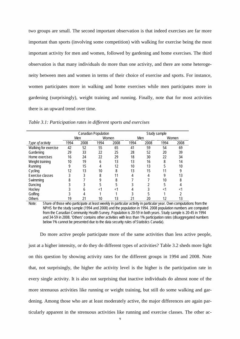
two groups are small. The second important observation is that indeed exercises are far more

important than sports (involving some competition) with walking for exercise being the most

important activity for men and women, followed by gardening and home exercises. The third

observation is that many individuals do more than one activity, and there are some heteroge-

neity between men and women in terms of their choice of exercise and sports. For instance,

women participates more in walking and home exercises while men participates more in

gardening (surprisingly), weight training and running. Finally, note that for most activities

there is an upward trend over time.

Table 3.1: Participation rates in different sports and exercises

Canadian Population Study sample Men Women Men Women Type of activity 1994 2008 1994 2008 1994 2008 1994 2008 Walking for exercise 42 52 55 65 41 59 54 69 Gardening 29 33 22 25 28 52 20 39 Home exercises 16 24 22 29 18 30 22 34 Weight training 10 19 6 13 13 16 8 14 Running 9 15 4 12 10 13 5 10 Cycling 12 13 10 8 13 15 11 9 Exercise classes 3 3 8 11 4 4 9 13 Swimming 8 7 9 8 7 7 10 8 Dancing 3 3 5 5 3 2 5 4 Hockey 3 6 <1 <1 4 3 <1 <1 Golfing 3 4 1 1 3 5 1 2 Others 19 21 10 13 21 20 12 13 Note: Share of those who participate at least weekly in particular activity in particular year. Own computations from the

NPHS for the study sample (1994 and 2008) and the population in 1994. 2008 population numbers are computed from the Canadian Community Health Survey. Population is 20-59 in both years. Study sample is 20-45 in 1994 and 34-59 in 2008. ‘Others’ contains other activities with less than 1% participation rates (disaggregated numbers below 1% cannot be presented due to the data security rules of Statistics Canada).

Do more active people participate more of the same activities than less active people,

just at a higher intensity, or do they do different types of activities? Table 3.2 sheds more light

on this question by showing activity rates for the different groups in 1994 and 2008. Note

that, not surprisingly, the higher the activity level is the higher is the participation rate in

every single activity. It is also not surprising that inactive individuals do almost none of the

more strenuous activities like running or weight training, but still do some walking and gar-

dening. Among those who are at least moderately active, the major differences are again par-

ticularly apparent in the strenuous activities like running and exercise classes. The other ac-

10

tivities show these differences as well, but less pronounced. In conclusion, moving from one

activity level to a more intensive one implies ‘more of the same’ as well as more emphasis on

more strenuous activities.

Table 3.2: Types of sports and exercises according to activity level in 1994 and 2008

Men Women 1994 2008 1994 2008 Type of activity Act Mod Inact Act Mod Inact Act Mod Inact Act Mod Inact Walking for exercise 66 58 25 85 69 36 82 79 40 90 83 52 Gardening 45 34 19 71 63 34 41 31 11 64 49 22 Home exercises 43 24 6 50 35 15 45 33 13 55 40 20 Weight training 35 18 2 36 14 5 25 15 1 29 19 4 Running 37 9 1 37 6 1 24 4 <1 29 9 2 Cycling 35 18 3 32 13 5 34 18 3 24 9 2 Exercise classes 12 5 <1 10 2 1 23 20 3 24 16 6 Swimming 14 12 3 11 10 3 29 16 4 18 9 2 Dancing 9 4 1 4 1 1 15 5 3 7 4 3 Hockey 9 6 1 8 4 <1 <1 <1 <1 1 <1 <1 Golfing 5 5 1 13 5 1 4 3 1 5 2 <1 Others 49 27 9 32 21 11 30 15 6 30 16 4 Note: Share of those who participate at least weekly in particular activity. Activity status is defined in respective year (Act:

active; Mod: moderately active; Inact: inactive). Own calculations based on study sample.

4 Towards a causal analysis: empirical research design

In this section, an empirical research design is discussed that arguably allows identify-

ing and estimating the causal effects of sports and exercise participation on labor market out-

comes without having to use instrumental variables. This is a big advantage, as it seems that

instruments which are at the same time valid and strong enough are not readily available in

this case. In order to derive this design, it is important first to recapitulate the findings of the

literature on the determinants and correlates of participation in sports and exercise.

4.1 Participation in sports and exercise

With respect to socio-economic characteristics, the literature finds that men are more

likely to participate in LTPA than women (e.g. Downward, 2007; Breuer and Wicker, 2008).9

9 Downward, Lera-López, and Rasciute (2011) contains a comprehensive survey of contributions of the correlates of

participation in sports and exercise. The following section heavily draws on this paper as well as on Lechner and Downward (2013).

11

Many studies also point to the importance of age, although there is no universal agreement on

the direction (and possible non-linearity) of its association with sports activities (e.g. Eberth

and Smith, 2010, Garcìa, Lera-López, and Suárez, 2011; Humphreys and Ruseski, 2010; Sta-

matakis and Chaudhury, 2008). Higher income raises the participation rate and frequency of

participation in sports and exercise (Downward and Rasciute, 2010; Humphreys and Ruseski,

2010; Lechner, 2009). The same is true for higher levels of education (e.g. Fridberg, 2010;

Hovemann and Wicker, 2009). A variety of household characteristics appears to reduce

participation in physical activity. These include being married and the presence of young

children in the household for females (Eberth and Smith, 2010; Garcìa, Lera-López, and

Suárez, 2011). Concerning employment characteristics, Downward (2004) finds a limited

association of working hours on participation. Meltzer and Jena (2010) show that the intensity

of exercise is positively associated with wage rates. Several studies also indicate that belong-

ing to an ethnic minority or being an immigrant is negatively associated with participation in

physical activities (e.g. Lechner, 2009a).

Further insights into the large physical activity literature are provided by the survey of

Bauman, Sallis, Dzewaltowski, and Owen (2002). They show that further variables may play

a role for doing sports and exercise as well. Such variables capture aspects of health, obesity,

and genetic factors, as well as psychological, cognitive, and emotional factors. In addition, it

seems that life style attributes associated with diet and smoking, as well as social and cultural

factors play a role.

Most of the factors mentioned above should be considered as confounding the relation

of sports and exercise participation and labor market outcomes. Thus, they need to be con-

trolled for in order to arrive at estimates that can be causally interpreted. Therefore, an im-

portant question is whether the data available for this study is rich enough to approximate

12

them.10 Beginning with the socio-economic factors, we observe age, sex, marital status, pres-

ence of young children in the household, immigration status, income, and education. We also

have proxy indicators for wealth measured as house ownership as well as size of the house (in

terms of the number of bedrooms). In particular, the number of bedrooms in one’s house may

provide a reasonable proxy (conditional on the number of children, etc.) for wealth. These

variables, therefore, cover key confounders of this group.

There are several indicators for individual labor market involvement, beyond income,

which capture general features of labor market participation, like employment status, as well

as particular features of the current job, like its sector or job position. A missing variable in

this group relates to the time intensity of the current job (i.e. working hours which is only

available in the post treatment period). Hopefully, this is captured by other variables availa-

ble, in particular by the type of occupation and the income generated.

Concerning variables describing the individual life styles, besides the variables on

sports and exercise, we observe alcohol consumption and smoking behavior in detail as well

as the BMI (computed using self-reported height and body weight). Thus, again, it is likely

that the key confounders in this group are observable. Furthermore, proxies for the intensity

of physical activities in daily life, other than sports and exercise, are available and used as fur-

ther control variables.

The data set used is unusually informative about health, which allows us to control for

objective and subjective health measures, as well as to distinguish between physical and

mental health and to take injuries into account.

Further, there are several regional indicators. The ones directly included in the analysis

characterize regions by population size and density, as well as by socio-economic features,

10 See Table A.1 in Appendix A for the details of all control variables used.

13

like average education and unemployment levels. Unfortunately, there is no direct information

on sports facilities available.

Finally, note that our econometric approach, to be explained in the next section, requires

conditioning on past activity levels (and lagged outcomes). This is also helpful for confounder

control, because if there are unobservable variables that have a time constant impact on

activity levels and labor market outcomes, like facilities for example, they will be captured by

the lagged activity and outcome levels (similar to a fixed effect in a panel regression).

4.2 A dynamic endogeneity problem

The previous section showed that due to the informative data set used there are little

concerns about unobservable confounding variables. Thus, an empirical approach using these

variables as control variables, like regression or matching type estimators do, should lead to

causal conclusions even when only a cross-section is used. One important condition for this to

hold, however, is that these variables are not influenced by the treatment (‘exogenous’ in this

particular sense)11. However, it is very likely that several, if not most, of the variables men-

tioned above are influenced by past sports and exercise participation. This effect could occur

contemporarily and / or after some time. This problem has already pointed out by Lechner

(2009a). Essentially, we follow his approach to tackle this issue by exploiting the panel

structure of the data.

4.3 Outline of the research design

The central ideas of the chosen research design are the followings: Firstly, in a group of

individuals who have the same activity level in a given year, by definition, this activity level

cannot differentially influence other variables measured at the same time for this group. Sec-

11 See Lechner (2008) for the necessary conditions in a non-parametric causal setting.

14

ondly, assuming that individuals do not decide on their sports and exercise activities accord-

ing to some long-term plan, which would imply all sorts of anticipating behavior that invali-

date almost any empirical analysis, future sports and exercise participation cannot have an

effect on the covariates measured before activity levels are decided.

These two considerations lead to the following empirical design: (i) Past activity levels

and confounders are measured in a base period (1994). (ii) Treatment is defined as the activity

level in the next period available (1996). (iii) Estimation is performed within each stratum

defined by the base period activity level, and the outcome variables are measured beginning

from 1996. (iv) Estimates obtained for the different strata are aggregated to obtain overall

effects. It is key to note that this set-up implies that within each stratum a conditional inde-

pendence assumption (selection-on-observables) is assumed to hold which in turn allows us-

ing methods that control for observable confounders (see Imbens, 2004, for necessary as-

sumptions and implications on estimation). Thus, there is no need to have instruments to

identify and estimate average causal effects.

One price to pay for this simplification is that the meaning of the treatment may be

somewhat different than in a standard non-dynamic or a fully dynamic setting (for which our

sample is too small). The reason is that, formally speaking, we estimate a one-time causal

effect of sports and exercise activity: In the base period, individuals are identical with respect

to their activity level. Essentially the effect of a change in that level is exploited with this ap-

proach. However, it will be shown in the next section that the current activity level has long

lasting effects on future activity levels. Therefore, the effects to be presented capture more

than contemporary, short term changes in activity levels. A more sophisticated alternative is

to define sequences of activity levels for several periods as the treatments. The problem of

this approach is that the confounders measured in the base period are unlikely to be good de-

terminants for decisions on activity levels several years ahead. To overcome this problem a

15

fully developed dynamic treatment approach may be used (e.g. Robins, 1986, Lechner, 2009b,

Lechner and Miquel, 2010, Lechner and Wiehler, 2013). However, such an approach when

implemented semiparametrically requires much larger samples than those available for this

study to get sufficiently precise estimates. Thus, it is not feasible with this data.

4.4 Implementation and descriptive statistics

We implement the basic ideas outlined above by using the three values of the activity

levels (inactive, moderately active, and active) in 1994 to define the strata. Given the evidence

in the literature that the selection for women and men into sports and exercise activities may

differ substantially (e.g. Andersen, 1995; Pate et al., 1995; or Sari, 2011, for Canada), the

activity states are interacted with sex to form six strata. Confounders are measured in 1994

while the treatment is defined as the activity status in the following period (1996).

4.4.1 Descriptive analysis

Table 4.1 shows descriptive statistics of some selected variables to better understand

how active, moderately active, and inactive individuals differ with respect to their character-

istics as well as later labor market outcomes (see Table A.1 in Appendix A for a comprehen-

sive list of variables). The first observation is that, because the table shows a snapshot at the

beginning of the panel data used, i.e. in 1994, individuals are on average still only about 33

years old (which is about the midpoint between 20 and 45, which defines the sample in 1994).

Concerning the personal characteristics, Table 4.1 shows that being male, having fewer young

children, and not being married (‘married’ includes having a common law partner), and hav-

ing a better education is positively associated with more activity.

The positive association of education and activity is also reflected in less active individ-

uals in a somewhat lower household income, a higher share of immigrants, and a smaller

share of people living in or close to big cities. Overall, the directions of the differences in the

16

socio-economic variables are in line, for example, with the results for Germany (Lechner,

2009a) or England (e.g. Lechner and Downward, 2013).

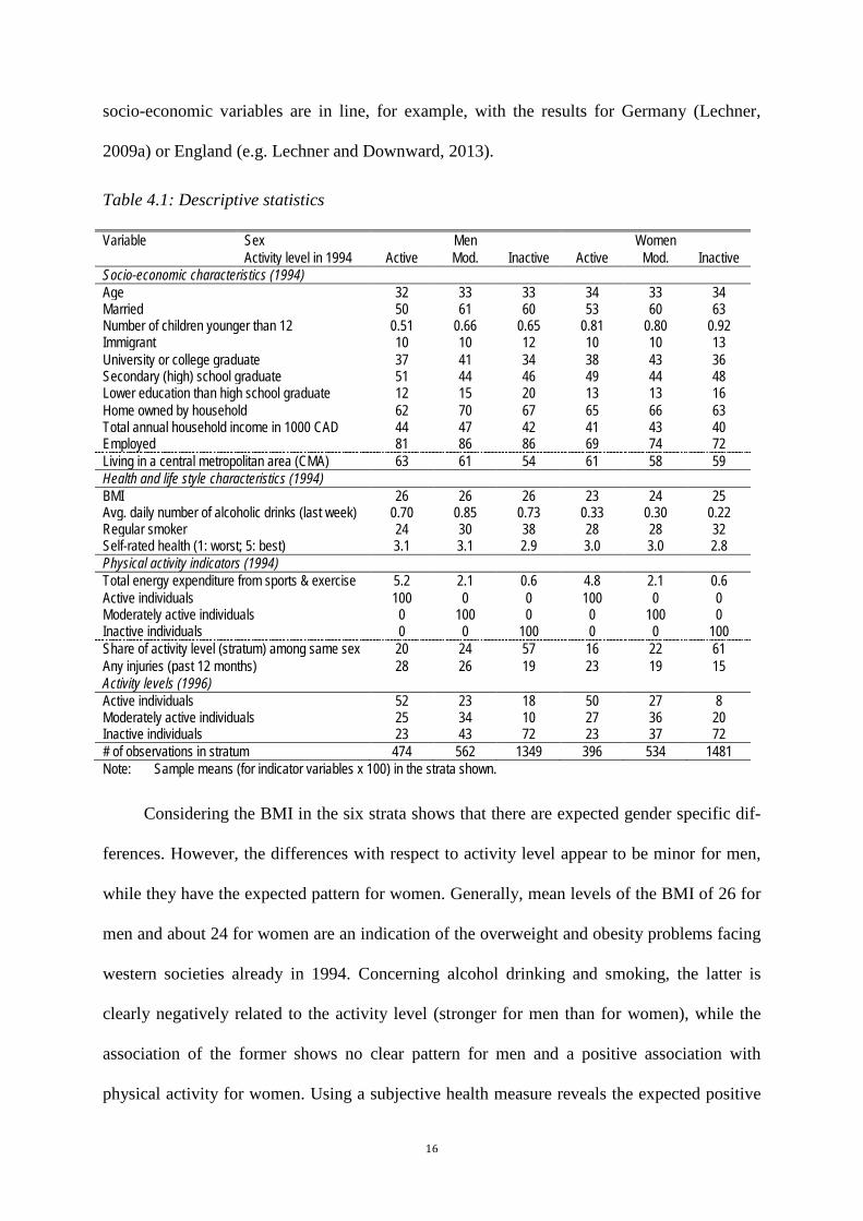
Table 4.1: Descriptive statistics

Variable Sex Men Women Activity level in 1994 Active Mod. Inactive Active Mod. Inactive

Socio-economic characteristics (1994) Age 32 33 33 34 33 34 Married 50 61 60 53 60 63 Number of children younger than 12 0.51 0.66 0.65 0.81 0.80 0.92 Immigrant 10 10 12 10 10 13 University or college graduate 37 41 34 38 43 36 Secondary (high) school graduate 51 44 46 49 44 48 Lower education than high school graduate 12 15 20 13 13 16 Home owned by household 62 70 67 65 66 63 Total annual household income in 1000 CAD 44 47 42 41 43 40 Employed 81 86 86 69 74 72 Living in a central metropolitan area (CMA) 63 61 54 61 58 59 Health and life style characteristics (1994) BMI 26 26 26 23 24 25 Avg. daily number of alcoholic drinks (last week) 0.70 0.85 0.73 0.33 0.30 0.22 Regular smoker 24 30 38 28 28 32 Self-rated health (1: worst; 5: best) 3.1 3.1 2.9 3.0 3.0 2.8 Physical activity indicators (1994) Total energy expenditure from sports & exercise 5.2 2.1 0.6 4.8 2.1 0.6 Active individuals 100 0 0 100 0 0 Moderately active individuals 0 100 0 0 100 0 Inactive individuals 0 0 100 0 0 100 Share of activity level (stratum) among same sex 20 24 57 16 22 61 Any injuries (past 12 months) 28 26 19 23 19 15 Activity levels (1996) Active individuals 52 23 18 50 27 8 Moderately active individuals 25 34 10 27 36 20 Inactive individuals 23 43 72 23 37 72 # of observations in stratum 474 562 1349 396 534 1481 Note: Sample means (for indicator variables x 100) in the strata shown.

Considering the BMI in the six strata shows that there are expected gender specific dif-

ferences. However, the differences with respect to activity level appear to be minor for men,

while they have the expected pattern for women. Generally, mean levels of the BMI of 26 for

men and about 24 for women are an indication of the overweight and obesity problems facing

western societies already in 1994. Concerning alcohol drinking and smoking, the latter is

clearly negatively related to the activity level (stronger for men than for women), while the

association of the former shows no clear pattern for men and a positive association with

physical activity for women. Using a subjective health measure reveals the expected positive

17

association between health and physical activity, which is also confirmed by more objective

health measures (for details see Table A.1 in Appendix A).

We consider measures of physical activities in 1994 and 1996 directly. Starting with

1994, the first observation concerns the relation of the three activity levels to the individual

overall expenditure of kilocalories burned due to LTPAs (as explained in Section 2). Here, in

addition, we see that active men are doing somewhat more strenuous activities than active

women. This is also confirmed in Section 3 based on participation differences in strenuous

activities between men and women. The second observation is the positive association be-

tween injuries and activity levels, which is of course not surprising, but rarely documented

(and a price to pay for doing sports and exercise).

Now, consider the overall number of individuals in the three activity levels. In 1994,

about 60% of men and women are inactive, while for the remaining part there are more mod-

erately active than active individuals. The last panels in Table 4.1 document the transition

from the activity levels in 1994 to those observed in 1996. 72% of the inactive individuals

remained inactive in 1996, while about 50% of the active remained active. However, while

very few inactive become active in 1996 almost one fourth of the active individuals in 1994

became inactive in 1996.

Finally, the last row in Table 4.1 shows the sample sizes for each stratum, which, of

course, influence the precision of the respective estimators to be discussed next.

4.4.2 Implementation

Within each stratum, propensity score matching using the estimator proposed by Lech-

ner, Miquel, and Wunsch (2011) is applied. This estimator performed well in the large-scale

simulation study by Huber, Wunsch, and Lechner (2013). It is described in detail in Appendix

C. Such semi-parametric estimators are based on estimating a parametric model (e.g. probit)

18

for the probability of belonging to one of the activity groups conditional on the above men-

tioned control variables. The relation between the outcomes, activity levels, and confounders,

however, are left completely unspecified (non-parametric). Therefore, such estimators have

the advantage of allowing for very flexible effect heterogeneity (contrary to regression mod-

els, for example).

For each outcome variable, this leads to six different estimates for each of the usual

treatment effects, like the average treatment effect (ATE), the average treatment effect on the

treated (ATET) and on the non-treated (ATENT). These effects can then either be used di-

rectly to describe the effects for the particular stratum or they may be aggregated to obtain

average effects for the subpopulation characterized by different activity levels, or for men and

women, or to obtain mean estimates for the population. The weights used here for aggregation

are proportional to the respective number of treated / controls / treated plus controls, depend-

ing on whether interest is in the ATET, ATENT, or the ATE. Since there are three possible

values of the treatment and since the conditional independence assumption is assumed to hold

within each stratum, the sample reduction results of Lechner (2001) apply. In other words to

estimate the effect of an activity status compared to another one, participants in the third state

are deleted for the purpose of this particular estimation. For example, for the estimation of the

effect of being active compared to being moderately active, inactive individuals play no role,

therefore not included in this particular estimation.

Most of this paper will take a dose-response perspective in the sense of estimating the

effect of changing the activity level from inactive to moderate and from moderate to active.

This perspective is possible in this study because of the detailed activity information available

in the data. Therefore, in order to implement the propensity score matching estimators for this

purpose in the six strata, twelve probit estimations are required; six for analyzing the active –

19

moderate contrast, and another six for analyzing the inactive – moderate contrast.12 The de-

tailed results of these estimations are reported in Appendix B (Tables B.1 and B.2).

The specifications of the probits follow the broad categories of variables shown in Table

4.1, but they include considerably more variables. For the sake of brevity, these twelve sets of

results are not discussed in detail.13 Overall, the probit estimates confirm the results of the

descriptive statistics discussed above pointing to effects of schooling, income, marriage,

previous life-style, health, and activity levels as well as regional indicators as correlates of the

activity level in the next period.14

5 Results

5.1 Dynamics of energy expenditure

The next step of the econometric analysis consists of understanding the relationship

between the treatment definitions in terms of the three activity levels and the energy ex-

penditure in the year of the treatment (1996) as well as for the later years.15 The corresponding

results are displayed in Figure 5.1. The vertical axis gives the changes in total energy ex-

penditure, while the horizontal axis indicates the year for which the effect is estimated. There

are estimates available for all odd years, which are linearly interpolated. The effects of the 12 Appendix D contains further comparisons like active – inactive or active together with moderately active versus inactive.

These comparisons require further probit estimations, which, however, we do not report for the sake of brevity.

13 Note that the estimation of those probits is merely a technical tool to flexibly capture and remove the influence of the covariates on the comparison of the treatment states. It is not their purpose to describe selection into treatment in a way that can be readily interpreted. To that end a less flexible but easier to interpret specification might be preferable which probably would not be estimated within the strata but on the overall sample.

14 When interpreting the results of the probit estimation keep in mind that estimation is within the six strata, so that the specifications are already conditional on sex and 1994 activity levels (similar to interacting all covariates with the six strata indicators in a joint estimation).

15 Alternatively, one could define a treatment over more than one period, but this would either raise the issue of missing confounders (if confounders measured in 1994 were used as only control variables), or raise the issue of endogenous confounders (if confounders after 1994 were also used as control variables, because they might be influenced by sport and exercise activities in 1996 and later).

20

treatment, i.e. an increase of the activity level by one level, are depicted by a solid line, while

the dashed lines show the 90% confidence bounds for the estimated effects. The effects are, of

course, allowed to differ for the two different treatments considered, namely inactive to mod-

erate (M-I; red with a rhombus) and moderate to active (A-M; blue with a square). All the

following figures are considering average treatment effects (ATE) for those who were moder-

ately active in 1994. In other words, we investigate what would happen to those moderately

active in 1994 if they increase, decrease, or continue their activity level. Appendix D presents

additional results for other populations and different effects that by and large confirm the

findings presented in the main body of the paper.

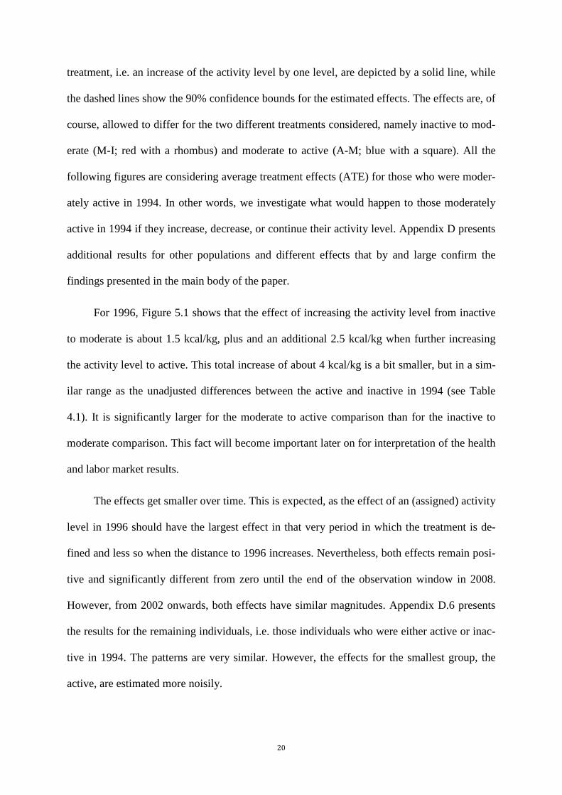
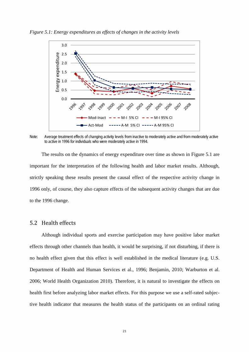
For 1996, Figure 5.1 shows that the effect of increasing the activity level from inactive

to moderate is about 1.5 kcal/kg, plus and an additional 2.5 kcal/kg when further increasing

the activity level to active. This total increase of about 4 kcal/kg is a bit smaller, but in a sim-

ilar range as the unadjusted differences between the active and inactive in 1994 (see Table

4.1). It is significantly larger for the moderate to active comparison than for the inactive to

moderate comparison. This fact will become important later on for interpretation of the health

and labor market results.

The effects get smaller over time. This is expected, as the effect of an (assigned) activity

level in 1996 should have the largest effect in that very period in which the treatment is de-

fined and less so when the distance to 1996 increases. Nevertheless, both effects remain posi-

tive and significantly different from zero until the end of the observation window in 2008.

However, from 2002 onwards, both effects have similar magnitudes. Appendix D.6 presents

the results for the remaining individuals, i.e. those individuals who were either active or inac-

tive in 1994. The patterns are very similar. However, the effects for the smallest group, the

active, are estimated more noisily.

21

Figure 5.1: Energy expenditures as effects of changes in the activity levels

Note: Average treatment effects of changing activity levels from inactive to moderately active and from moderately active

to active in 1996 for individuals who were moderately active in 1994.

The results on the dynamics of energy expenditure over time as shown in Figure 5.1 are

important for the interpretation of the following health and labor market results. Although,

strictly speaking these results present the causal effect of the respective activity change in

1996 only, of course, they also capture effects of the subsequent activity changes that are due

to the 1996 change.

5.2 Health effects

Although individual sports and exercise participation may have positive labor market

effects through other channels than health, it would be surprising, if not disturbing, if there is

no health effect given that this effect is well established in the medical literature (e.g. U.S.

Department of Health and Human Services et al., 1996; Benjamin, 2010; Warburton et al.

2006; World Health Organization 2010). Therefore, it is natural to investigate the effects on

health first before analyzing labor market effects. For this purpose we use a self-rated subjec-

tive health indicator that measures the health status of the participants on an ordinal rating

0.0

0.5

1.0

1.5

2.0

2.5

3.0

Ener

gy e

xpen

ditu

re

Mod-Inact M-I 5% CI M-I 95% CI

Act-Mod A-M 5% CI A-M 95% CI

22

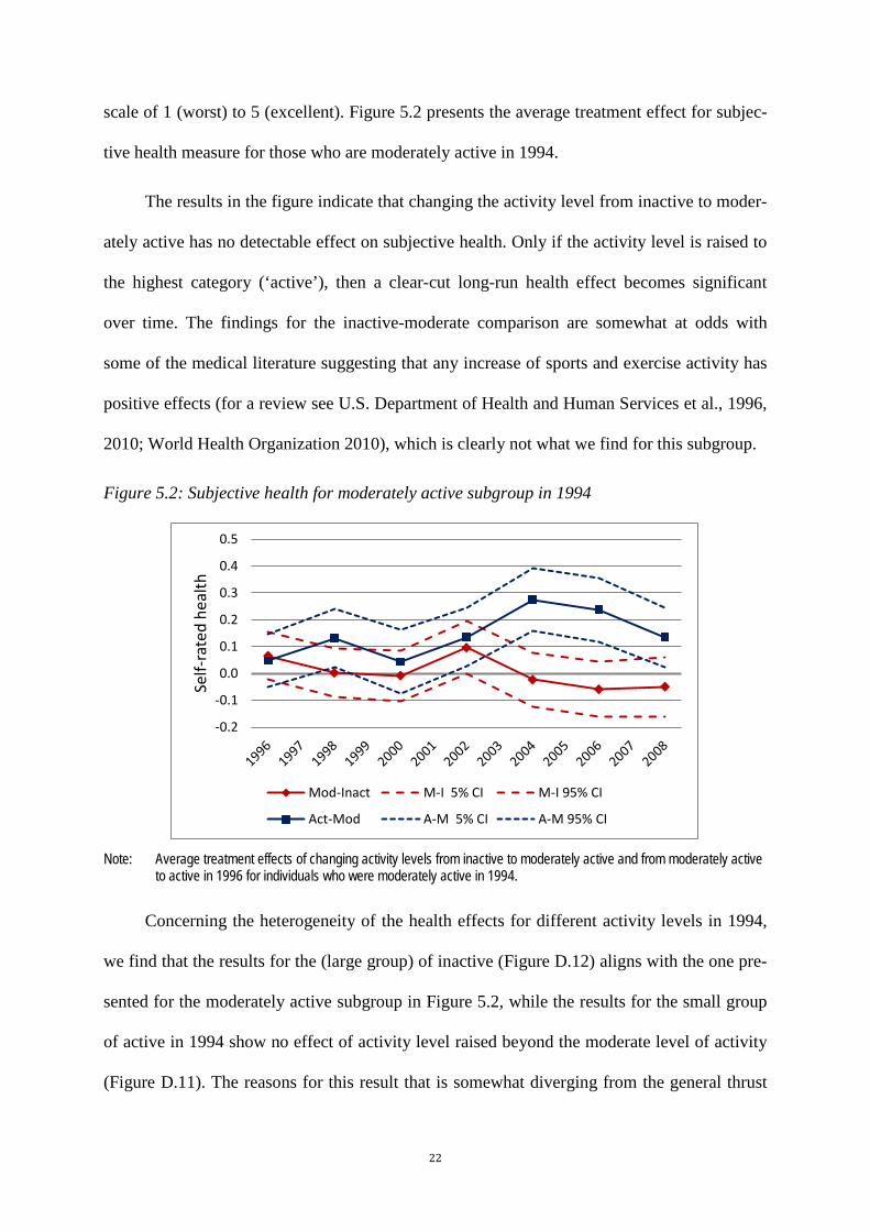
scale of 1 (worst) to 5 (excellent). Figure 5.2 presents the average treatment effect for subjec-

tive health measure for those who are moderately active in 1994.

The results in the figure indicate that changing the activity level from inactive to moder-

ately active has no detectable effect on subjective health. Only if the activity level is raised to

the highest category (‘active’), then a clear-cut long-run health effect becomes significant

over time. The findings for the inactive-moderate comparison are somewhat at odds with

some of the medical literature suggesting that any increase of sports and exercise activity has

positive effects (for a review see U.S. Department of Health and Human Services et al., 1996,

2010; World Health Organization 2010), which is clearly not what we find for this subgroup.

Figure 5.2: Subjective health for moderately active subgroup in 1994

Note: Average treatment effects of changing activity levels from inactive to moderately active and from moderately active

to active in 1996 for individuals who were moderately active in 1994.

Concerning the heterogeneity of the health effects for different activity levels in 1994,

we find that the results for the (large group) of inactive (Figure D.12) aligns with the one pre-

sented for the moderately active subgroup in Figure 5.2, while the results for the small group

of active in 1994 show no effect of activity level raised beyond the moderate level of activity

(Figure D.11). The reasons for this result that is somewhat diverging from the general thrust

-0.2

-0.1

0.0

0.1

0.2

0.3

0.4

0.5

Self-

rate

d he

alth

Mod-Inact M-I 5% CI M-I 95% CI

Act-Mod A-M 5% CI A-M 95% CI

23

of the other results remain an issue for further research. A companion paper, Sari and Lechner

(2014), contains a considerably more detailed analysis of the health effects.

5.3 Labor market effects

In this section, the effects of increased sports and exercise participation on individual

and household earnings as well as other labor market indicators, like working hours and em-

ployment status are discussed. The main results, i.e. the ATE for the moderately active sub-

sample, are given within this section, while additional results are relegated to Appendix D.

5.3.1 Personal income

Figure 5.3 shows the results for ‘annual personal income’ and contains the main results

of this paper: Over time, there are positive effects on earnings for an activity increase from

moderate to active, but the increase from inactivity to only a moderate sports and exercise

activity is too small to generate such effects. This finding is more or less in line with the ef-

fects for subjective health shown in the previous section.

Figure 5.3 suggests that it takes some time before the effects materialize (remember that

treated and controls have the same distribution of activity levels in 1994), but eventually the

effects become large enough to be significant. Figure D.1 in Appendix D relates the effects to

the underlying levels of earnings that could be achieved under the different treatments. They

are all increasing over time (and / or with age) and reach 60’000 to 65’000 CAD in 2008.16

This suggests effects of around 10 to 20% after 8 to 12 years. This is somewhat larger than the

values reported by Lechner (2009a) for Germany (but his study was based on a far less so-

16 Note that due to sample attrition the samples get smaller over time and thus the estimates become noisier.

24

phisticated dataset). The effects for the moderate-inactive comparison are positive as well, but

considerably smaller and not statistically significant.17

Figure 5.3: Annual personal income

Note: Average treatment effects of changing activity levels from inactive to moderately active and from moderately active

to active in 1996 for individuals who were moderately active in 1994.

Figure 5.4: Annual average personal income

Note: Numbers shown in year x are the average effects over the years from 1996 to year x. Average treatment effects of

changing activity levels from inactive to moderately active and from moderately active to active in 1996 for individu-als who were moderately active in 1994.

17 Note that these earnings effects are based on nominal CAD. Figure D.19 deflates the effects to 2002 CAD. The resulting

differences are minor.

-10'000

-5'000

0

5'000

10'000

15'000

20'000

Annu

al p

erso

nal i

ncom

e in

CAD

Mod-Inact M-I 5% CI M-I 95% CI

Act-Mod A-M 5% CI A-M 95% CI

-10'000

-5'000

0

5'000

10'000

15'000

20'000

1996

1997

1998

1999

2000

2001

2002

2003

2004

2005

2006

2007

2008

Annu

al a

vera

ge p

erso

nal i

ncom

e in

CAD

Mod-Inact M-I 5% CI M-I 95% CI

Act-Mod A-M 5% CI A-M 95% CI

25

Instead of looking at the gain in annual earnings in every year, one may average the

earnings differences from 1996 onwards to get an overall average of gains up to a particular

year.18 Figure 5.4 shows that the conclusions do not change by using this accumulated out-

come variable instead. In the long run, there are average gains in personal income from in-

creasing the activity level from moderate to active of more than 10%. These gains are consid-

erably smaller, if positive at all, when the increase is only from inactive to moderate.

Appendices D.2 to D.7 contain heterogeneity and robustness checks for these findings.

In Appendix D.2, different treatment comparisons are performed, like comparing the active

directly to the inactive, and pooling the active and moderately active treatments to contrast

them to the inactive (Figures D.2 and D.3). Both comparisons confirm the general findings

explained above (although with less precision).

In Appendix D.3, the effects are compared for the same subpopulation. This means that

instead of comparing the two ATEs (as shown above), the ATENT for the active vs. moderate

contrast is compared to the ATET of the moderate vs. inactive contrast. Thus, both parameters

refer to the same population of individuals who are moderately active in 1996 (and 1994).

Again, the general findings (Figures D.4 and D.5) outlined above are confirmed.

Finally, instead of considering only individuals who are moderately active in 1994, the

ATE’s of the six strata are aggregated to obtain an overall average effect for the population

(Figure D.6 in Appendix D.4). Again, the previous results are confirmed for the active-mod-

erate comparison (although effects appear to be a little smaller). However, for the moderate-

inactive comparisons, some effects for the later years could not be computed because of sam-

ple size problems in some subpopulations.

18 Such estimation uses averages over time and individuals. Thus, it will be more precise which is reflected in the somewhat

narrower confidence bounds.

26

Do the results differ for men and women and for the different activity states in 1994?

For the active-moderate comparison (Figure D.7, D.8 in Appendix D.5), the effects for men

and women are similar. The moderate-inactive comparison, however, suggests that while ef-

fects for women may be absent, for men they may be in the same range as for the active-

moderate contrast. However, as before the estimations for women are subject to the sample

size problems mentioned above. With respect to activity levels in 1994, there does not appear

to be much effect heterogeneity, so that the qualitative general findings are again confirmed

(Figures D.9 to D.14 in Appendix D.6).

Finally, the income concept is broadened from personal income to household income

(Figures D.15 and D.16 in Appendix D.7). Again, the same pattern arises although the effects

seem to be somewhat larger in magnitude (perhaps due to a likely positive correlation of sport

activities of the adult members of a household).

5.3.2 Employment

Next, results for variables indicating whether somebody is employed at all or full-time

employed, as well as for a measure of working hours are considered.

The employment effects for the two comparisons exhibit a distinctly different dynamic

pattern (Figure 5.5). For the active-moderate comparison, there is first a decline of employ-

ment followed by an increase, while for the moderate-inactive comparison the pattern is ex-

actly opposite. This suggests that for 1998 to about 2002 changes from either active or inac-

tive to a moderate activity level increases employment. This could be the case if a further in-

crease of sports and exercise activities beyond a moderate level increases the value of leisure

time (respectively, sports and exercise just take more time to conduct and is not a complete

substitute with other leisure activities). This would reflect the nature of active sports and exer-

cise participations as a consumption good complementary to leisure. Thus, rational individu-

als would reduce employment almost immediately and increase their leisure time while also

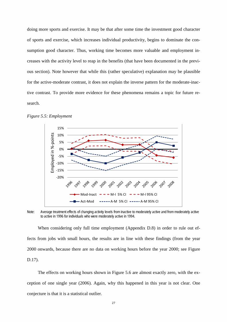
27

doing more sports and exercise. It may be that after some time the investment good character

of sports and exercise, which increases individual productivity, begins to dominate the con-

sumption good character. Thus, working time becomes more valuable and employment in-

creases with the activity level to reap in the benefits (that have been documented in the previ-

ous section). Note however that while this (rather speculative) explanation may be plausible

for the active-moderate contrast, it does not explain the inverse pattern for the moderate-inac-

tive contrast. To provide more evidence for these phenomena remains a topic for future re-

search.

Figure 5.5: Employment

Note: Average treatment effects of changing activity levels from inactive to moderately active and from moderately active

to active in 1996 for individuals who were moderately active in 1994.

When considering only full time employment (Appendix D.8) in order to rule out ef-

fects from jobs with small hours, the results are in line with these findings (from the year

2000 onwards, because there are no data on working hours before the year 2000; see Figure

D.17).

The effects on working hours shown in Figure 5.6 are almost exactly zero, with the ex-

ception of one single year (2006). Again, why this happened in this year is not clear. One

conjecture is that it is a statistical outlier.

-20%

-15%

-10%

-5%

0%

5%

10%

15%

Empl

oyed

in %

-poi

nts

Mod-Inact M-I 5% CI M-I 95% CI

Act-Mod A-M 5% CI A-M 95% CI

28

Figure 5.6: Working hours

Note: Working hours are computed as annual hours / 52. Hours of non-employed workers are set to 0. Information on

annual hours is available from 2000 onwards. Average treatment effects of changing activity levels from inactive to moderately active and from moderately active to active in 1996 for individuals who were moderately active in 1994.

5.4 Further sensitivity checks

The previous section already mentioned several sensitivity checks conducted with re-

spect to the key earnings results. A further concern is the effect that attrition may have on the

results presented above. As with every panel study based on survey data, there is the issue of

panel attrition (on top of item non-response). If attrition is confounding, i.e. jointly related to

treatment and selection, then it may invalidate the attempted causal inference. Due to the

selection of the sample, the panel is balanced in the first two periods. After 1996, attrition

occurs. The impact of the later attrition can be checked (to some extent) by using the full

sample and estimating an effect for an additional outcome variable which is defined as one if

nonresponse occurs and zero otherwise (for details see Appendix C.2). With the single excep-

tion of the year 2000, the results of this exercise (Figure C.1) reveal no evidence for selective

(confounding) attrition.

A further implicit overall check of the plausibility of the chosen approach is to see

whether the effects follow a plausible dynamic pattern. Given that the treatment consists of

-6

-4

-2

0

2

4

6

8

Wee

kly

hour

s

Mod-Inact M-I 5% CI M-I 95% CI

Act-Mod A-M 5% CI A-M 95% CI

29

comparing different activity levels in 1996 conditional on having the same activity level in

1994 (while leaving the period after 1996 unrestricted), it would be very surprising to see

immediate labor market effects (of this investment in health and social capital), other than

perhaps some employment reduction due to increased value of leisure which may occur im-

mediately. This is of course not true for subjective health which may plausibly show a short-

term as well as a long term effect. Comparing the results across the various figures reveals no

compelling evidence for implausible dynamic patterns. The exception is perhaps the evolve-

ment of the employment effect which has been discussed above.

6 Conclusion

In this study we investigated the medium and long term effects of sports and exercise on

labor market outcome for working age adults. The empirical analysis is based on Canadian

panel data that are particularly suitable for such an analysis because they are unusually in-

formative about sports and exercise, about potential confounding variables such as health and

life style, and they contain labor market outcomes as well. The informative data set is used

with a research design based on stratification and semi-parametric matching estimation that

arguably allows the causal interpretation of the resulting estimates.

We find robust positive earnings effects that increase to more than 10% after some

years, which broadly compares to the returns of one to two years of schooling (e.g. Card,

1999). Interestingly, an important heterogeneity appears in the sense that only increasing the

level of sports and exercise activity to a level higher than the one recommended by national

and international health organizations has this clear-cut impact. Smaller increases appear to

have only a minor impact that is hard to pin with the sample sizes available in this study.

Interesting further research may address this heterogeneity issue: A possible, but of

course speculative, explanation of this heterogeneity may be that activity is measured subjec-

30

tively. From other studies it is known that individuals may exaggerate their physical activity

(e.g. Sebastiao et al., 2012).19 Furthermore, another interesting dimension of sports and exer-

cise is the heterogeneity with respect to different types of activity, as different types of sports

foster different skills that are valuable in the labor market.

References

Ainsworth, B. E., W. L. Haskell, M. C. Whitt, M. L. Irwin, A. M. Swartz, S. J. Strath, W. L. O'Brien, D. R. Bas-

sett, Jr., K. H. Schmitz, P. O. Emplaincourt, D. R. Jacobs, Jr., and A. S. Leon (2000). Compendium of Physi-

cal Activities: An Update of Activity Codes and MET Intensities, Medicine and Science in Sports and Exer-

cise, 32 (9S), S498-S516.

Andersen, R. M. (1995). Revisiting the Behavioral Model and Access to Medical Care: Does it Matter?, Journal

of Health and Social Behavior, 36 (1), 1-10.

Bauman, A. E., J. F. Sallis, D. A. Dzewaltowski, and N. Owen (2002). Toward a Better Understanding of the

Influences on Physical Activity: The Role of Determinants, Correlates, Causal Variables, Mediators, Moder-

ators, and Confounders, American Journal of Preventive Medicine, 23 (2S), 5-14.

Benjamin, R. M. (2010). The Surgeon General’s Vision for a Healthy and Fit Nation, Public Health Reports, 125

(4), 514-515.

Breuer, C., and P. Wicker (2008). Demographic and Economic Factors Influencing Inclusion in the German

Sport System. A Microanalysis of the Years 1985 to 2005, European Journal for Sport and Society, 5 (1), 33-

42.

Card, David (1999): "The Causal Effect of Education on Earnings", Handbook of Labour Economics 3A, ch. 30,

1801-1863.

Cornelißen, T., and C. Pfeifer (2008). Sport und Arbeitseinkommen - Individuelle Ertragsraten von

Sportaktivitäten in Deutschland, Jahrbuch für Wirtschaftswissenschaften (Review of Economics), 59 (3), 244-

255.

Canadian Society for Exercise Physiology (CSEP). 2013. Canadian Physical Activity Guidelines. Also available

at www.csep.ca/guidelines. Accessed August 22, 2013.

Downward, P. M. (2004). Assessing Neoclassical Microeconomic Theory via Leisure Demand: A Post Keynes-

ian Perspective, Journal of Post Keynesian Economics, 26 (3), 371-395.

Downward, P. M. (2007). Exploring the Economic Choice to Participate in Sport: Results from the 2002 General

Household Survey, The International Review of Applied Economics, 21 (5), 633-653.

Downward, P. M., and S. Rasciute (2010). The Relative Demands for Sports and Leisure in England, European

Sports Management Quarterly, 10 (2), 189-214.

19 Although, the way Statistics Canada computes the calorie expenditures takes this measurement issue to some extend into

account.

31

Downward, P. M., F. Lera-Lopez, and S. Rasciute (2011). The Economic Analysis of Sports Participation in

Robinson, L., Bodet, G., and Downward, P. (eds.), International Handbook of Sports Management, London:

Routledge.

Eberth, B., and M. Smith, (2010). Modelling the Participation Decision and Duration of Sporting Activity in

Scotland, Economic Modelling, 27 (4), 822-834.

EU (2013). Impact Assessment - Accompanying the Document, Proposal for a Council Recommendation on

Promoting Health-Enhancing Physical Activity across Sectors.

Furlong W.J., D.H. Feeny, G.W. Torrance (1999). Health Utilities Index (HUI): Algorithm for determining HUI

Mark 2 (HUI2)/Mark 3 (HUI3) health status classification levels, health states, health-related quality of life

utility scores and single-attribute utility score from 40-item interviewer-administered health status question-

naires. Dundas, Canada: Health Utilities Inc. February 1999.

Fridberg, T. (2010). Sport and Exercise in Denmark, Scandinavia and Europe, Sport in Society, 13 (4), 583-592.

García, J., F. Lera-López, and M. J. Suárez (2011). Estimation of a Structural Model of the Determinants of the

Time Spent on Physical Activity and Sport: Evidence for Spain, Journal of Sports Economics, 12 (5), 515-

537.

Haskell, W. L., I. M. Lee, R. R. Pate, K. E. Powell, S. N. Blaire, B. A. Franklyn, C. A. Macera, G. W. Heath, P.

D. Thompson, and A. Bauman (2007). Physical Activity and Public Health: Updated Recommendation for

Adults from the American College of Sports Medicine and the American Heart Association, Medicine and

Science in Sports and Exercise, 39 (8), 1423-1434.

Hovemann, G., and P. Wicker (2009). Determinants of Sport Participation in the European Union, European

Journal for Sport and Society, 6 (1), 51-59.

Huber, M., M. Lechner, and A. Steinmayr (2012). Radius Matching on the Propensity Score with Bias Adjust-

ment: Finite Sample Behaviour, Tuning Parameters and Software Implementation, Economics Working Pa-

per Series 1226, University of St. Gallen, School of Economics and Political Science.

Huber, M., M. Lechner, and C. Wunsch (2013). The performance of estimators based on the propensity score,

Journal of Econometrics, 175, 1-21.

Humphreys B. R., and J. E. Ruseski (2010). The Economic Choice of Participation and Time Spent in Physical

Activity and Sport in Canada, Working Paper No 2010-14, Department of Economics, University of Alberta.

Humphreys, B. R., L. McLeod, and J. E. Ruseski (2014). Physical Activity and Health Outcomes: Evidence from

Canada, Health Economics, 23 (1), 33-54.

Imbens, G. W. (2004). Nonparametric Estimation of Average Treatment Effects under Exogeneity: A Review,

The Review of Economics and Statistics, 86, 4-29.

Kavetsos, G. (2011). The Impact of Physical Activity on Employment, The Journal of Socio-Economics, 40,

775-779.

Lechner, M. (2001). Identification and Estimation of Causal Effects of Multiple Treatments under the Condi-

tional Independence Assumption, in M. Lechner, F. Pfeiffer (eds.), Econometric Evaluation of Labour Mar-

ket Policies, Heidelberg: Physica, 43-58.

Lechner, M. (2009a). Long-Run Labour Market and Health Effects of Individual Sports Activities, The Journal

of Health Economics, 28, 839-854.

32

Lechner, M. (2009b). Sequential Causal Models for the Evaluation of Labor Market Programs, Journal of Busi-

ness & Economic Statistics, 27, 71-83.

Lechner, M. (2008). A Note on Endogenous Control Variables in Causal Studies, Statistics and Probability

Letters, 78, 190-195.

Lechner, M., and P. Downward (2013). Heterogeneous Sports Participation and Labour Market Outcomes in

England, Discussion Paper No. 2013-25, Department of Economics, University of St. Gallen.

Lechner, M., and R. Miquel (2010). Identification of the Effects of Dynamic Treatments by Sequential Condi-

tional Independence Assumptions, Empirical Economics, 39, 111-137.

Lechner, M., and S. Wiehler (2013). Does the Order and Timing of Active Labor Market Programs Matter?,

Oxford Bulletin of Economics and Statistics, 72 (2), 180-212.

Lechner, M., R. Miquel, and C. Wunsch (2011). Long-Run Effects of Public Sector Sponsored Training in West

Germany, Journal of the European Economic Association, 9, 742-784.

Liu J., T. Wade, B.E. Faught, J. Hay. (2008). Physical inactivity in Canada: Results from the Canadian

Community Health Survey Cycle 2.2 (2004-2005). Public Health 122, 1384-1386

Meltzer, D. O., and A. B. Jena (2010). The Economics of Intense Exercise, Journal of Health Economics, 29,

347-352.

Pate R. R., M. Pratt, S. N. Blair, W.L. Haskell, C.A. Macera, C. Bouchard, D. Buchner, W. Ettinger, G.W.

Heath, A. C. King, A. Kriska, A. S. Leon, B. H. Marcus, J. Morris, R. S. Paffenbarger, K. Patrick, M. L.

Pollock, J.M. Rippe, J. Sallis, and J. H. Wilmore (1995). Physical Activity and Public Health: A Recommen-

dation from the Centers for Disease Control and Prevention and the American College of Sports Medicine.

Journal of the American Medical Association, 273, 402-407.

Reiner, M., C. Niermann, D. Jekauc, and A. Woll (2013). Long-Term Health Benefits of Physical Activity – a

Systematic Review of Longitudinal Studies, BMC Public Health, 13, 813.

Robins, J. M. (1986). A New Approach to Causal Inference in Mortality Studies with Sustained Exposure Peri-

ods - Application to Control of the Healthy Worker Survivor Effect, Mathematical Modelling, 7, 1393-1512.

Rooth, D.-O. (2011). Work out or Out of Work: The Labour Market Return to Physical Fitness and Leisure and

Sport Activities, Labour Economics, 18, 399-409.

Sari, N. (2010). A short walk a day shortens the hospital stay: Physical activity and the demand for hospital ser-

vices for older adults, Canadian Journal of Public Health, 101 (5), 385-389.

Sari, N. (2009). Physical inactivity and its impact on healthcare utilization, Health Economics, 18 (8), 885-901

Sari, N. (2011). Does Physical Exercise Affect Demand for Hospital Services? Evidence from Canadian Panel

Data in P. R. Guerrero, S. Kesenne, and B. R. Humphreys (eds), The Economics of Sport, Health and Happi-

ness: The Promotion of Well-being through Sporting Activities, Northampton: Edward Elgar, 81-100.

Sari, N. (2013). Sports, exercise and length of stay in hospitals: Is there a differential effect for chronically ill

people? Contemporary Economic Policy (forthcoming) doi:10.1111/coep.12028.

Sari, N., and M. Lechner (2014). Long-run health effects of sports and exercise in Canada, mimeo.

33

Sebastiao, E., S. Gobbi, W. Chodzko-Zajko, A. Schwingel, C. B. Papini, P. M. Nakamura, A. V. Netto, E. Ko-

kubun (2012). The International Physical Activity Questionnaire-Long Form Overestimates Self-Reported

Physical Activity of Brazilian Adults, Public Health, 126, 967-975.

Seippel, Ø. (2006). Sport and Social Capital, Acta Sociologica, 49 (2), 169-193.

Stamatakis, E., and M. Chaudhury (2008). Temporal Trends in Adults’ Sports Participation Patterns in England

between 1997 and 2006: The Health Survey for England, British Journal of Sports Medicine, 42, 901-908.

Tambay, J.-L., and G. Catlin (1995). Sample Design of the National Population Health Survey, Health Reports,

7 (1), 29-38.

U.S. Department of Health and Human Services, Centers for Disease Control and Prevention, National Center

for Chronic Disease Prevention and Health Promotion, and The President’s Council on Physical Fitness and

Sports (1996). The Effects of Physical Activity on Health and Disease, Physical Activity and Health: A Re-

port of the Surgeon General, 81-172.

U.S. Department of Health and Human Services (2008). Physical Activity Guidelines Advisory Committee Re-

port, 2008.

Warburton, D., C. W. Nicol, and S. S. D. Bredin (2006). Health Benefits of Physical Activity: The Evidence,

Canadian Medical Association Journal, 174 (6), 801-809.

World Health Organization (2010). Global Recommendations on Physical Activity for Health, WHO Press: Ge-

neva, Switzerland.

34

Appendix A: Descriptive statistics

Table A.1: Descriptive statistics for the strata

Variable Men Women Activity level in 1994 Active Moderate Inactive Active Moderate Inactive

Age 31.9 33.3 33.2 33.5 33.1 33.7 Married/common law partner 0.50 0.61 0.60 0.53 0.60 0.63 Number of children of age < 12 0.51 0.66 0.65 0.81 0.80 0.92 Immigrant 0.10 0.10 0.12 0.10 0.10 0.13 University / college graduate 0.37 0.41 0.34 0.38 0.43 0.36 Secondary school graduate 0.51 0.44 0.46 0.49 0.44 0.48 Average daily # of alcohol consumption (past week) 0.70 0.85 0.73 0.33 0.30 0.22 Daily alcohol drinker (last year) 0.03 0.04 0.04 0.02 0.02 0.01 2-6 times per week alcohol drinker (last year) 0.31 0.34 0.27 0.15 0.13 0.10 Body mass index (BMI) 25.7 25.8 25.9 23.4 24.1 24.5 Regular smoker 0.24 0.30 0.38 0.28 0.28 0.32 Self-rated health (1: worst; 5: best) 3.12 3.06 2.89 3.03 3.04 2.83 Health utility index (HUI) 0.91 0.91 0.89 0.91 0.90 0.88 Depression scale 0.42 0.36 0.29 0.68 0.68 0.69 Activities prevented by pain 0.06 0.06 0.06 0.08 0.07 0.11 Distress scale 3.20 3.24 3.35 3.45 3.78 4.16 At least one of the 5 chronic conditions 0.04 0.04 0.05 0.06 0.05 0.06 Other chronic conditions 0.40 0.41 0.36 0.47 0.46 0.46 Home owned by household 0.62 0.70 0.67 0.65 0.66 0.63 Number of bedrooms in home 2.68 2.86 2.76 2.89 2.84 2.90 Total annual household income in 1000

CAD 43.8 46.8 41.7 40.7 43.3 39.8 Employed 0.81 0.86 0.86 0.69 0.74 0.72 Occupation in management, business, finance, administration, sciences 0.23 0.24 0.22 0.24 0.26 0.29

Usually sit during daily activities 0.16 0.21 0.19 0.15 0.19 0.23 Total energy expenditure from leisure time physical activities 5.15 2.10 0.56 4.80 2.07 0.57 Not biking in non-leisure time 0.80 0.88 0.93 0.86 0.91 0.96 Not walking in non-leisure time 0.43 0.43 0.50 0.31 0.32 0.38 Injuries other than repetitive strain injuries (past 12 months) 0.28 0.26 0.19 0.23 0.19 0.15

Male 25+ unemployment rate 0.09 0.09 0.10 0.09 0.09 0.10 Highest schooling rate 15+ aged: Less than grade 9 0.11 0.12 0.13 0.11 0.12 0.13 Log of regional population density -5.98 -5.72 -5.47 -5.70 -5.64 -5.74 Central metropolitan area 0.63 0.61 0.54 0.61 0.58 0.59 Share of active 1996 0.52 0.23 0.18 0.50 0.27 0.08 Share of moderate 1996 0.25 0.34 0.10 0.27 0.36 0.20 Share of inactive 1996 0.23 0.43 0.72 0.23 0.38 0.73 Observations 474 562 1349 396 534 1481 Note: Sample means shown. If not mentioned otherwise, all variables are measured in 1994. HUI is a quality adjusted

health status indicator which describes an individual’s overall functional health with a single numerical value for any possible combination of levels of eight self-reported health attributes (vision, hearing, speech, mobility, dexterity, cognition, emotion, and pain and discomfort). For a detailed explanation, see Furlong, Feeny, and Torrance (1999).

35

Appendix B: Results of probit estimation

Tables B.1 and B.2 show the coefficients of the probit estimation for the active vs. mod-

erate as well as the moderate vs. inactive comparisons.

Table B.1: Coefficients of probit estimations for active vs. moderately active comparison

Variable Men Women Activity level in 1994 Active Moderate Inactive Active Moderate Inactive

Age -0.008 -0.008 -0.003 -0.010 -0.024 -0.017 Married / common law partner 0.072 0.032 0.116 -0.003 0.142 0.276 Number of children of age < 12 -0.031 -0.134 0.015 -0.012 0.047 0.011 Immigrant 0.296 0.409 0.135 0.278 -0.016 0.124 University / college graduate 0.047 -0.213 -0.201 -0.312 0.142 -0.176 Secondary school graduate -0.293 0.025 -0.118 -0.393 -0.275 -0.234 Average daily # of alcohol consumption (past week) -0.150 -0.093 -0.001 -0.003 -0.039 0.225

2-6 times or daily per week alcohol drinker (last year) -0.251 0.023 0.105 0.548 -0.260 -0.084 BMI -0.004 -0.012 0.007 -0.017 -0.030 -0.024 Regular smoker -0.028 -0.105 -0.022 -0.267 0.497 0.108 Self-rated health -0.056 -0.031 0.000 -0.075 -0.117 0.007 Health utility index -0.906 -0.770 -0.376 -0.217 -0.594 0.437 Depression scale -0.014 0.113 0.021 0.033 -0.050 -0.076 Activities prevented by pain -0.090 0.189 -0.032 0.018 0.149 0.340 Distress scale -0.042 -0.025 0.029 -0.017 0.016 0.010 At least one of the 5 chronic conditions -0.120 -0.381 -0.670 -0.355 -0.356 -0.238 Other chronic conditions -0.018 0.076 -0.172 -0.009 -0.137 0.075 Home owned by household 0.095 -0.283 -0.092 0.342 -0.156 0.033 Number of bedrooms in home 0.012 0.161 0.011 -0.121 0.021 0.085 Total household income/10000 -0.003 -0.054 0.002 0.078 -0.006 -0.060 Employed 0.433 -0.047 -0.023 0.336 -0.365 0.106 Not in labor force - - - 0.003 -0.439 0.057 Occupation in management, business, finance, administration, sciences 0.224 0.235 -0.093 -0.020 -0.194 -0.128

Usually sit during daily activities 0.165 -0.155 -0.428 -0.193 -0.246 0.102 Total energy expenditure from leisure time physical activities 0.156 0.192 0.173 0.079 0.293 0.255 Not biking in non-leisure time -0.309 0.018 -0.048 -0.085 -0.246 -0.039 Not walking in non-leisure time 0.014 -0.150 -0.070 -0.001 -0.250 -0.259 Injuries other than repetitive Strain injuries (past 12 months) 0.197 -0.030 0.048 0.594 0.173 0.029

Male 25+ unemployment rate 1.197 0.587 0.723 3.322 1.513 -4.222 Highest schooling rate 15+ aged: Less than grade 9 2.388 -0.285 0.774 -1.695 -3.196 0.369 Log of regional pop. density -0.019 -0.050 -0.006 -0.015 0.025 0.070 Central metropolitan area 0.284 0.109 0.109 -0.326 -0.299 0.232 Efron’s Pseudo R2 in % 13.8 10.2 5.1 12.8 15.0 9.0 Note: All covariates are measured in 1994. Numbers in bold italics / bold / italics denote significance at the 1% / 5% /

10% level. All specifications include a constant term. Dependent variable is ‘active in 1996’. Sample consists of ac-tive and moderately active individuals (1996).

36

Table B.2: Coefficients of probit estimations for the moderate vs. inactive comparison

Variable Men Women Activity level in 1994 Active Moderate Inactive Active Moderate Inactive

Age 0.023 0.001 -0.005 -0.001 -0.012 -0.004 Married / common law partner -0.035 -0.155 0.043 -0.525 -0.079 -0.205 Number of children of age < 12 0.018 -0.006 0.012 0.010 -0.040 -0.046 Immigrant -0.074 -0.119 -0.136 -0.394 0.292 -0.301 University / college graduate 0.487 0.046 -0.083 0.213 0.053 -0.185 Secondary school graduate 0.752 -0.136 0.066 -0.040 0.247 0.049 Average daily # of alcohol consumption (past week) -0.100 -0.014 -0.043 0.176 -0.087 -0.011 2-6 times or daily per week alcohol drinker (last year) 0.132 -0.115 -0.126 -0.359 0.067 0.190 BMI -0.006 -0.013 -0.003 -0.007 0.001 -0.002 Regular smoker -0.340 -0.031 -0.005 0.156 -0.232 0.010 Self-rated health 0.328 -0.014 0.019 0.296 0.095 0.013 Health utility index -1.239 0.603 0.194 1.464 1.449 0.304 Depression scale -0.103 -0.110 -0.082 -0.068 -0.013 0.009 Activities prevented by pain -0.263 -0.052 0.392 0.612 0.790 -0.158 Distress scale -0.005 0.004 0.002 0.008 -0.006 -0.011 At least one of the 5 chronic conditions 0.474 0.053 0.028 0.109 0.078 -0.226 Other chronic conditions 0.110 0.091 0.022 0.223 0.059 -0.055 Home owned by household 0.043 0.489 0.114 -0.052 0.228 0.068 Number of bedrooms in home -0.070 -0.163 -0.055 -0.095 0.010 -0.049 Total annual household income/10000 0.030 0.070 0.022 0.007 0.003 0.048 Employed -0.167 0.153 -0.081 -0.209 0.270 0.201 Not in labor force - - - 0.160 0.076 0.354 Occupation in management, business, finance, administration, sciences -0.260 -0.194 -0.102 0.564 -0.119 0.040

Usually sit during daily activities 0.034 0.009 0.152 0.452 -0.238 0.000 Total energy expenditure from leisure time physical activities -0.018 0.433 0.649 -0.017 0.079 0.612 Not biking in non-leisure time 0.097 0.001 -0.005 -0.382 0.022 0.143 Not walking in non-leisure time -0.290 -0.072 -0.150 -0.038 -0.116 0.021 Injuries other than repetitive Strain injuries (past 12 months) -0.028 -0.153 0.006 -0.361 0.013 0.236

Male 25+ unemployment rate -0.020 -1.595 0.112 -2.469 -1.651 0.328 Highest schooling rate 15+ aged: Less than grade 9 -3.188 -0.690 -1.129 -2.835 1.978 -0.543 Log of regional population density 0.047 0.028 -0.042 0.075 0.016 -0.046 Central metropolitan area -0.052 0.005 -0.187 0.041 0.185 -0.136 Efron’s Pseudo R2 in % 14.0 10.1 6.5 18.0 7.8 6.5 Note: All covariates are measured in 1994. Numbers in bold italics / bold / italics denote significance at the 1% / 5% /

10% level. All specifications include a constant term. Dependent variable is ‘moderately active in 1996’. Sample consists of moderately active or inactive individuals (1996).

37

Appendix C: Econometric issues

Appendix C.1: The matching estimator

Table C.1 gives the detailed matching protocol used. See Huber, Lechner, and Wunsch

(2013) and Huber, Lechner, and Steinmayr (2012) for further details on the implementation

and the properties of this estimator, including trimming and common support rules.

Table C.1: Matching protocol for the estimation of a counterfactual outcome and the effects

Step A-1 Choose one observation in the subsample defined by d=1 and delete it from that pool. Step B-1 Find an observation in the subsample defined by d=0 that is as close as possible to the one chosen in step A-

1) in terms of (𝑥), 𝑥�. 'Closeness' is based on the Mahalanobis distance. Step C-1 Repeat A-1) and B-1) until no observation with d=1 is left. Step D-1 Compute the maximum distance (dist) obtained for any comparison between a member of the reference

distribution and matched comparison observations. Step A-2 Repeat A-1). Step B-2 Repeat B-1). If possible, find other observations in the subsample of d=0 that are at least as close as R * dist

to the one chosen in step A-2). Do not remove these observations, so that they can be used again. Compute weights for all chosen comparisons observations that are proportional to their distance. Normalise the weights such that they add to one.

Step C-2 Repeat A-2) and B-2) until no participant in d=1 is left. Step D-2 D-2) For any potential comparison observation, add the weights obtained in A-2) and B-2). Step E Using the weights 𝑤(𝑥𝑖) obtained in D-2), run a weighted linear regression of the outcome variable on the

variables used to define the distance (and an intercept). Step F-1 Predict the potential outcome 𝑦0(𝑥𝑖) of every observation using the coefficients of this regression: 𝑦�0(𝑥𝑖) . Step F-2 Estimate the bias of the matching estimator for 𝐸(𝑌0|𝐷 = 1) as: ∑ (1−𝑑𝑖)𝑤𝑖𝑦�0(𝑥𝑖)

𝑁0− 𝑑𝑖𝑦�0(𝑥𝑖)

𝑁1𝑁𝑖=1 .

Step G Using the weights obtained by weighted matching in D-2), compute a weighted mean of the outcome vari-ables in d=0. Subtract the bias from this estimate to get 𝐸(𝑌0|𝐷 = 1).

Note: R is set to 150%. Age is used as additional matching variable ( x ). The weight of the propensity score coming from the Mahalanobis metric is multiplied by 5. Control observations with weights larger than 5% are removed.

Table C.1 shows how to compute the average treatment effects on the treated (ATET).

The average treatment effects on the non-treated (ATENT) are computed in the same way but

the role of treated and controls are reversed in the algorithm. The average treatment effect

(ATE) is computed by aggregating both effects using the treatment share (ATE = ATET x

P(D=1) + ATENT x P(D=0)). These estimations are performed for each of the six subsamples

separately. The weights used to aggregate these estimates over specific groups or the popula-

tion are proportional to the number of treated (for the ATET) / controls (ATENT) / popula-

tions (ATE) in the respective subsamples.

38

Inference is based on the ‘approximate’ asymptotic standard errors as explained and in-

vestigated in Lechner (2002). The basic idea is that the matching weights are treated as non-

stochastic. In Lechner (2002), this approach appears to lead to conservative inference. Unfor-

tunately, the infrastructure of the RDC (with which all computations had to be performed due

to data security concerns for the particular data used) did not allow us to obtain bootstrap in-

ference based on a sufficiently large number of bootstrap replications. For the active and

moderate subsample of men in the active-inactive comparison, we did however obtain 99

bootstrap replications. Comparing standard errors estimated from the 99 bootstraps suggests

that the approximate asymptotic standard errors are not far off, sometimes being somewhat

smaller or somewhat larger than the (still rather noisily estimated) bootstrap standard errors.

Appendix C.2: Panel attrition

The sample used is an unbalanced panel for which we require complete answers to all

variables used by the probit, i.e. only for the years 1994 and 1996. The results presented for

the later years are based on those cases with valid information for the particular outcome vari-

able shown.

The number of people answering the survey decreases from one cycle to the next due to

attrition caused by non-response (refusals, individuals that were untraceable or partial re-

sponse; deceased or institutionalized persons are counted as a response for longitudinal pur-

poses). Out of 17,276 individuals in Cycle 1, the gross panel response rate is 93.6% in Cycle

2, 88.9% in Cycle 3, and decreased to 77.6% in Cycle 6, and further to 70.7% in Cycle 8.

Refusal is the largest source of non-response in the NPHS. Based on surveys that were

sent out to panel members, the refusal rate increased from 3.1% in Cycle 2 to 6.3% in Cycle

4. However, it stabilized around 8% for the remaining Cycles of the NPHS. After refusal, the

failure to trace a longitudinal panel member is the second most important source of non-re-

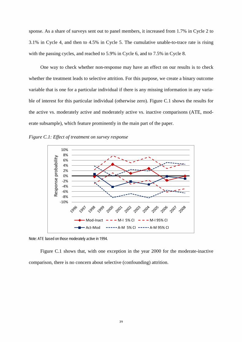
39

sponse. As a share of surveys sent out to panel members, it increased from 1.7% in Cycle 2 to

3.1% in Cycle 4, and then to 4.5% in Cycle 5. The cumulative unable-to-trace rate is rising

with the passing cycles, and reached to 5.9% in Cycle 6, and to 7.5% in Cycle 8.

One way to check whether non-response may have an effect on our results is to check

whether the treatment leads to selective attrition. For this purpose, we create a binary outcome

variable that is one for a particular individual if there is any missing information in any varia-

ble of interest for this particular individual (otherwise zero). Figure C.1 shows the results for

the active vs. moderately active and moderately active vs. inactive comparisons (ATE, mod-

erate subsample), which feature prominently in the main part of the paper.

Figure C.1: Effect of treatment on survey response

Note: ATE based on those moderately active in 1994.

Figure C.1 shows that, with one exception in the year 2000 for the moderate-inactive

comparison, there is no concern about selective (confounding) attrition.

-10%-8%-6%-4%-2%0%2%4%6%8%

10%

Resp

onse

pro

babi

lity

Mod-Inact M-I 5% CI M-I 95% CI

Act-Mod A-M 5% CI A-M 95% CI

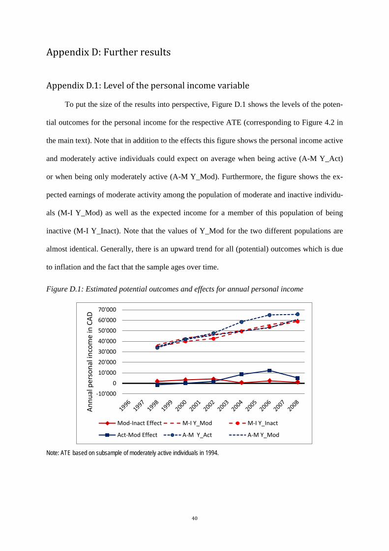
40

Appendix D: Further results

Appendix D.1: Level of the personal income variable

To put the size of the results into perspective, Figure D.1 shows the levels of the poten-

tial outcomes for the personal income for the respective ATE (corresponding to Figure 4.2 in

the main text). Note that in addition to the effects this figure shows the personal income active

and moderately active individuals could expect on average when being active (A-M Y_Act)

or when being only moderately active (A-M Y_Mod). Furthermore, the figure shows the ex-

pected earnings of moderate activity among the population of moderate and inactive individu-

als (M-I Y_Mod) as well as the expected income for a member of this population of being

inactive (M-I Y_Inact). Note that the values of Y_Mod for the two different populations are

almost identical. Generally, there is an upward trend for all (potential) outcomes which is due

to inflation and the fact that the sample ages over time.

Figure D.1: Estimated potential outcomes and effects for annual personal income

Note: ATE based on subsample of moderately active individuals in 1994.

-10'000

0

10'000

20'000

30'000

40'000

50'000

60'000

70'000

Annu

al p

erso

nal i

ncom

e in

CAD

Mod-Inact Effect M-I Y_Mod M-I Y_Inact

Act-Mod Effect A-M Y_Act A-M Y_Mod

41

Appendix D.2: Results aggregated over different activity states in period 1

Figure D.2: Annual personal income: Active vs. inactive and active & moderate vs. inactive

Note: ATE based on subsample of moderately active individuals in 1994.

Figure D.3: Average annual personal income: Active vs. inactive and active & moderate vs.

inactive

Note: ATE based on subsample of moderately active individuals in 1994.

Figure D.2 shows the results for the ATE of personal income when active and moderate

activities are compared to inactivity and when being active is directly compared to being in-

active. Effects are positive in both cases. However, they are only at the boarder of being sig-

-10'000

-5'000

0

5'000

10'000

15'000

20'000An

nual

per

sona

l inc

ome

in C

AD

Act-Inact M-I 5% CI M-I 95% CI

Act/Mod-Inact A-M 5% CI A-M 95% CI

-10'000

-5'000

0

5'000

10'000

15'000

20'000

Annu

al p

erso

nal i

ncom

e in

CAD

Act-Inact M-I 5% CI M-I 95% CI

Act/Mod-Inact A-M 5% CI A-M 95% CI

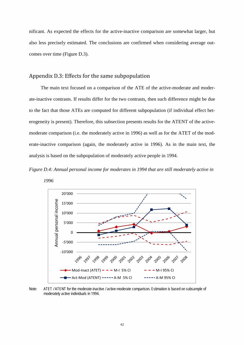
42

nificant. As expected the effects for the active-inactive comparison are somewhat larger, but

also less precisely estimated. The conclusions are confirmed when considering average out-

comes over time (Figure D.3).

Appendix D.3: Effects for the same subpopulation

The main text focused on a comparison of the ATE of the active-moderate and moder-

ate-inactive contrasts. If results differ for the two contrasts, then such difference might be due

to the fact that those ATEs are computed for different subpopulation (if individual effect het-

erogeneity is present). Therefore, this subsection presents results for the ATENT of the active-

moderate comparison (i.e. the moderately active in 1996) as well as for the ATET of the mod-

erate-inactive comparison (again, the moderately active in 1996). As in the main text, the

analysis is based on the subpopulation of moderately active people in 1994.

Figure D.4: Annual personal income for moderates in 1994 that are still moderately active in

1996

Note: ATET / ATENT for the moderate-inactive / active-moderate comparison. Estimation is based on subsample of

moderately active individuals in 1994.

-10'000

-5'000

0

5'000

10'000

15'000

20'000

Annu

al p

erso

nal i

ncom

e

Mod-Inact (ATET) M-I 5% CI M-I 95% CI

Act-Mod (ATENT) A-M 5% CI A-M 95% CI

43

Figure D.5: Average annual personal income for moderates in 1994 that are still moderately

active in 1996

Note: ATET / ATENT for the moderate-inactive / active-moderate comparison. Estimation is based on subsample of

moderately active individuals in 1994.

Qualitatively, the results reflect the same patterns as for the ATE shown in the main

body of the paper.

Appendix D.4: Averages over all subpopulations

Most of the results presented so far focused on the population with a moderate activity

level in 1994. Figure D.6 presents the results aggregated over all 1994 activity levels. It ap-

pears that the effects become stronger for the active-moderate comparisons, while no effects

are detectable for the moderate-inactive comparison.

-10'000

-5'000

0

5'000

10'000

15'000

20'000An

nual

per

sona

l inc

ome

Mod-Inact (ATET) M-I 5% CI M-I 95% CI

Act-Mod (ATENT) A-M 5% CI A-M 95% CI

44

Figure D.6: Annual personal income: ATE aggregated over activity states in 1994

Note: The results for the moderate-inactive comparison extend only to 2004, because the female active (1994)

subpopulation responding to this income question and observed to be inactive is too small afterwards.

Appendix D.5: Gender heterogeneity

Figure D.7 and D.8 show gender difference based on the ATE aggregated over all 1994

activity populations. The results suggest that the effects for men are somewhat more pro-

nounced than for women, although the differences between the point estimates are hardly sig-

nificant.

-10'000

-5'000

0

5'000

10'000

15'000

20'000

Annu

al a

vera

ge p

erso

nal i

ncom

e in

CAD

Mod-Inact M-I 5% CI M-I 95% CI

Act-Mod A-M 5% CI A-M 95% CI

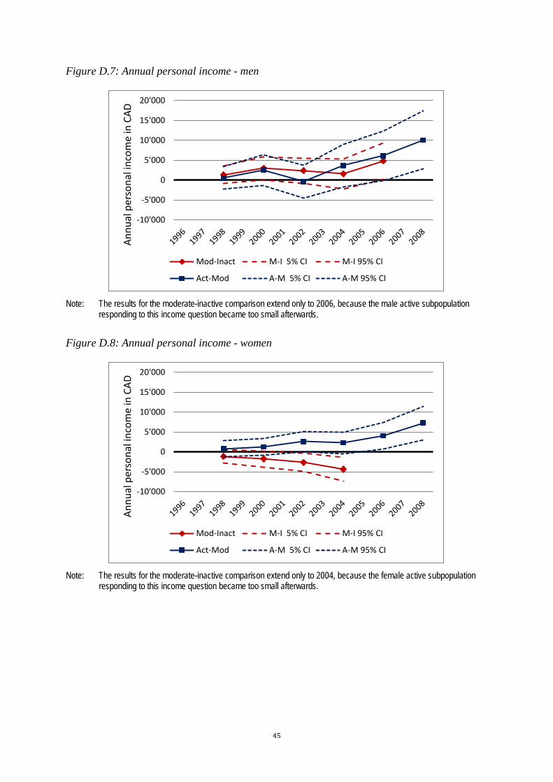
45

Figure D.7: Annual personal income - men

Note: The results for the moderate-inactive comparison extend only to 2006, because the male active subpopulation

responding to this income question became too small afterwards.

Figure D.8: Annual personal income - women

Note: The results for the moderate-inactive comparison extend only to 2004, because the female active subpopulation

responding to this income question became too small afterwards.

-10'000

-5'000

0

5'000

10'000

15'000

20'000

Annu

al p

erso

nal i

ncom

e in

CAD

Mod-Inact M-I 5% CI M-I 95% CI

Act-Mod A-M 5% CI A-M 95% CI

-10'000

-5'000

0

5'000

10'000

15'000

20'000

Annu

al p

erso

nal i

ncom

e in

CAD

Mod-Inact M-I 5% CI M-I 95% CI

Act-Mod A-M 5% CI A-M 95% CI

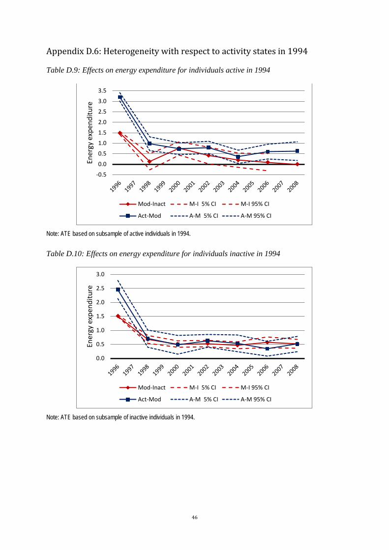
46

Appendix D.6: Heterogeneity with respect to activity states in 1994

Table D.9: Effects on energy expenditure for individuals active in 1994

Note: ATE based on subsample of active individuals in 1994.

Table D.10: Effects on energy expenditure for individuals inactive in 1994

Note: ATE based on subsample of inactive individuals in 1994.

-0.5

0.0

0.5

1.0

1.5

2.0

2.5

3.0

3.5En

ergy

exp

endi

ture

Mod-Inact M-I 5% CI M-I 95% CI

Act-Mod A-M 5% CI A-M 95% CI

0.0

0.5

1.0

1.5

2.0

2.5

3.0

Ener

gy e

xpen

ditu

re

Mod-Inact M-I 5% CI M-I 95% CI

Act-Mod A-M 5% CI A-M 95% CI

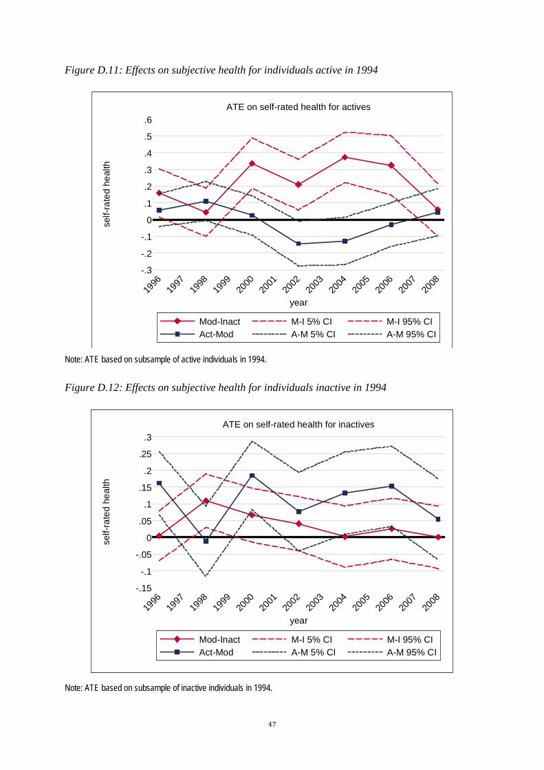
47

Figure D.11: Effects on subjective health for individuals active in 1994

Note: ATE based on subsample of active individuals in 1994.

Figure D.12: Effects on subjective health for individuals inactive in 1994

Note: ATE based on subsample of inactive individuals in 1994.

-.3

-.2

-.1

0

.1

.2

.3

.4

.5

.6se

lf-ra

ted

heal

th

1996

1997

1998

1999

2000

2001

2002

2003

2004

2005

2006

2007

2008

year

Mod-Inact M-I 5% CI M-I 95% CIAct-Mod A-M 5% CI A-M 95% CI

ATE on self-rated health for actives

-.15

-.1

-.05

0

.05

.1

.15

.2

.25

.3

self-

rate

d he

alth

1996

1997

1998

1999

2000

2001

2002

2003

2004

2005

2006

2007

2008

year

Mod-Inact M-I 5% CI M-I 95% CIAct-Mod A-M 5% CI A-M 95% CI

ATE on self-rated health for inactives

48

Considering the effects for the different subsamples (Figures D.13, D.14, 5.3) confirms

the view that it is difficult to detect any effect from becoming moderately active, but that there

is a large gain from changing from being moderately active to being active. However, com-

paring the effects over the three activity states in 1994 does not reveal much heterogeneity

(taking into account sampling uncertainty).

Figure D.13: Effects on annual personal income for individuals active in 1994

Note: ATE based on subsample of active individuals in 1994.

Figure D.14: Effects on annual personal income for individuals inactive in 1994

Note: ATE based on subsample of inactive individuals in 1994.

-10'000

-5'000

0

5'000

10'000

15'000

20'000

Annu

al p

erso

nal i

ncom

e in

CAD

Mod-Inact M-I 5% CI M-I 95% CI

Act-Mod A-M 5% CI A-M 95% CI

-10'000

-5'000

0

5'000

10'000

15'000

20'000

Annu

al p

erso

nal i

ncom

e in

CAD

Mod-Inact M-I 5% CI M-I 95% CI

Act-Mod A-M 5% CI A-M 95% CI

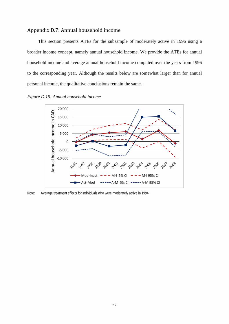
49

Appendix D.7: Annual household income

This section presents ATEs for the subsample of moderately active in 1996 using a

broader income concept, namely annual household income. We provide the ATEs for annual

household income and average annual household income computed over the years from 1996

to the corresponding year. Although the results below are somewhat larger than for annual

personal income, the qualitative conclusions remain the same.

Figure D.15: Annual household income

Note: Average treatment effects for individuals who were moderately active in 1994.

-10'000

-5'000

0

5'000

10'000

15'000

20'000

Annu

al h

ouse

hold

inco

me

in C

AD

Mod-Inact M-I 5% CI M-I 95% CI

Act-Mod A-M 5% CI A-M 95% CI

50

Figure D.16: Annual average household income

Note: Numbers shown in year x are the average effects for the outcomes over the years from1996 to year x. Average

treatment effects for individuals who were moderately active in 1994.

Appendix D.8: Full time employment

This section presents ATEs for the subsample of moderately active in 1994 for full time

employment (defined as annual hours / 52 larger than 35; Figure D.17). The information on

annual working hours is not available before 2000. For 2000 and later, the patterns roughly

coincide with those observed for employment, which are discussed in the main body of text.

-10'000

-5'000

0

5'000

10'000

15'000

20'000

1996

1997

1998

1999

2000

2001

2002

2003

2004

2005

2006

2007

2008

Annu

al a

vg. h

ouse

hold

inco

me

in

CAD

Mod-Inact M-I 5% CI M-I 95% CI

Act-Mod A-M 5% CI A-M 95% CI

51

Figure D.17: Full time employment

Note: Full time employment is defined as working more than 35 hours. Information on annual hours is available from

2000 onwards. Average treatment effects for individuals who were moderately active in 1994.

Figure D.18: Annual personal income in 2002 CAD

Note: Deflated using the GDP price deflator with base year 2002. Average treatment effects for individuals who were

moderately active in 1994

-10%

-5%

0%

5%

10%

15%

Full

time

empl

oyed

in %

-poi

nts

Mod-Inact M-I 5% CI M-I 95% CI

Act-Mod A-M 5% CI A-M 95% CI

-10000

-5000

0

5000

10000

15000

20000

25000

Annu

al p

erso

nal i

ncom

e in

CAD

Mod-Inact M-I 5% CI M-I 95% CI

Act-Mod A-M 5% CI A-M 95% CI