The Schreier-Sims algorithm

An essay

submitted to the Department of mathematics,

Australian National University,

in partial fulfillment of the requirements

for the degree of

Bachelor of Science with Honours

By

Scott H. Murray

November 2003

Acknowledgements

I would like to thank my supervisor Dr E.A. O’Brien, who has been a constant

source of help and encouragement.

I am also grateful to Dr John Cannon of Sydney University and Professor

Cheryl E. Praeger of the University of Western Australia for enlightening dis-

cussions on aspects of this project.

Abstract

A base and strong generating set provides an effective computer representation

for a permutation group. This representation helps us to calculate the group

order, list the group elements, generate random elements, test for group mem-

bership and store group elements efficiently. Knowledge of a base and strong

generating set essentially reduces these tasks to the calculation of certain orbits.

Given an arbitrary generating set for a permutation group, the Schreier-

Sims algorithm calculates a base and strong generating set. We describe several

variations of this method, including the Todd-Coxeter, random and extending

Schreier-Sims algorithms.

Matrix groups over finite fields can also be represented by a base and strong

generating set, by considering their action on the underlying vector space. A

practical implementation of the random Schreier-Sims algorithm for matrix

groups is described. We investigate the effectiveness of this implementation

for computing with soluble groups, almost simple groups, simple groups and

related constructions.

We consider in detail several aspects of the implementation of the random

Schreier-Sims algorithm. In particular, we examine the generation of random

group elements and choice of “stopping condition”. The main difficulty in apply-

ing this algorithm to matrix groups is that the orbits which must be calculated

are often very large. Shorter orbits can be found by extending the point set to

include certain subspaces of the underlying vector space. We demonstrate that

even greater improvements in the performance of the random Schreier-Sims al-

gorithm can be achieved by using the orbits of eigenvectors and eigenspaces of

the generators of the group.

Contents

1 Background and notation 1

1.1 An overview . . . . . . . . . . . . . . . . . . . . . . . . . . . . . 1

1.2 Notation . . . . . . . . . . . . . . . . . . . . . . . . . . . . . . . 3

1.3 Coset enumeration . . . . . . . . . . . . . . . . . . . . . . . . . 5

2 Fundamental concepts 9

2.1 Chains of subgroups . . . . . . . . . . . . . . . . . . . . . . . . 9

2.2 Bases and strong generating sets . . . . . . . . . . . . . . . . . . 11

2.3 Orbits and Schreier structures . . . . . . . . . . . . . . . . . . . 13

2.4 Computing orbits . . . . . . . . . . . . . . . . . . . . . . . . . . 19

2.5 Testing group membership . . . . . . . . . . . . . . . . . . . . . 20

2.6 Representing group elements . . . . . . . . . . . . . . . . . . . . 22

3 The Schreier-Sims algorithm 25

3.1 Partial BSGS and Schreier’s lemma . . . . . . . . . . . . . . . . 25

3.2 The Schreier-Sims algorithm . . . . . . . . . . . . . . . . . . . . 30

3.3 The Todd-Coxeter Schreier-Sims algorithm . . . . . . . . . . . . 34

3.4 The random Schreier-Sims algorithm . . . . . . . . . . . . . . . 36

3.5 The extending Schreier-Sims algorithm . . . . . . . . . . . . . . 37

3.6 Choice of algorithm . . . . . . . . . . . . . . . . . . . . . . . . . 39

4 The random Schreier-Sims algorithm for matrices 41

4.1 Conversion to matrix groups . . . . . . . . . . . . . . . . . . . . 41

4.2 Orbits and Schreier structures . . . . . . . . . . . . . . . . . . . 43

4.3 Implementations . . . . . . . . . . . . . . . . . . . . . . . . . . 45

4.4 Evaluating performance . . . . . . . . . . . . . . . . . . . . . . 47

5 Investigating performance 50

5.1 Random elements . . . . . . . . . . . . . . . . . . . . . . . . . . 50

5.2 Stopping conditions . . . . . . . . . . . . . . . . . . . . . . . . . 54

5.3 Point sets . . . . . . . . . . . . . . . . . . . . . . . . . . . . . . 57

5.4 Eigenvectors and eigenspaces . . . . . . . . . . . . . . . . . . . . 62

References . . . . . . . . . . . . . . . . . . . . . . . . . . . . . . . . . 67

Index 70

Chapter 1

Background and notation

1.1 An overview

The design of algorithms for computing with finite permutation groups has been

a particularly successful area of research within computational group theory.

Such algorithms played an important part in the classification of the finite simple

groups and have applications in other areas of mathematics, such as graph theory

and combinatorics. An introduction to permutation group algorithms can be

found in Butler (1991) and a recent survey of computational group theory is

provided by Cannon & Havas (1992).

Successful computing with a permutation group is largely dependent on our

ability to find an effective representation for the group. In particular, many cal-

culations can be facilitated if we have a descending chain of subgroups, together

with a set of coset representatives for each subgroup of the chain in its prede-

cessor. We can construct a chain in which each subgroup is a point stabiliser of

the last. The sequence of points stabilised is called a base, and a set containing

generators for each subgroup in the chain is called a strong generating set; these

concepts were introduced by Sims (1971) as an effective description of a permu-

tation group. Sets of coset representatives for this chain can be constructed by

calculating orbits of the base points. In Chapter 2, we define these concepts more

formally and describe their fundamental applications, which include calculating

the order of a group and testing for group membership. Our construction of the

sets of coset representatives combines the new concept of a Schreier structure

with ideas from earlier descriptions, such as Leon (1991) and Butler (1986).

1

Given a group described by generating permutations, the Schreier-Sims algo-

rithm constructs a base and strong generating set for it. This algorithm was first

described in Sims (1970) and uses Schreier’s lemma to find generating sets for

the stabilisers. However, these sets usually contain many redundant generators,

so variations of the algorithm have been developed which reduce the number

of generators which are considered. The Todd-Coxeter Schreier-Sims algorithm

(Sims, 1978) uses coset enumeration to calculate the index of one stabiliser in

its predecessor, and so determine if we have a complete generating set; coset

enumeration is briefly described in Section 1.3. The random Schreier-Sims algo-

rithm (Leon, 1980b) uses random elements, rather than Schreier generators, to

construct a probable base and strong generating set. We can then use the Todd-

Coxeter Schreier-Sims algorithm (among others) to verify that this probable base

and strong generating set is complete. The extending Schreier-Sims algorithm

(Butler, 1979) efficiently constructs a base and strong generating set for certain

subgroups of interest. All of these algorithms are described in Chapter 3.

Many of the algorithms which have been developed for matrix groups over

finite fields are modifications of permutation group algorithms. In particular, we

can represent a matrix group by a base and strong generating set, if we consider

its natural action on the underlying vector space. In Chapter 4, we describe

the theory behind such modifications and discuss Schreier structures for matrix

groups. The algorithms in Chapter 3 were first implemented for matrix groups by

Butler (1976; 1979). As part of this project a new implementation of the random

Schreier-Sims algorithm has been developed. We investigate the effectiveness of

this implementation with soluble groups, almost simple groups, simple groups

and related constructions.

In Chapter 5, we consider issues related to the implementation of the ran-

dom Schreier-Sims algorithm. First, we study generating random elements of a

group, a fundamental task in computational group theory. We briefly discuss

methods suggested in the literature, and compare the impact of different gen-

eration schemes on our implementation. Next, we discuss conditions which are

used to terminate the random Schreier-Sims algorithm. The three most common

stopping conditions are compared in detail for the first time.

The main difficulty with using the random Schreier-Sims algorithm for ma-

trix groups is that the base points often have very large orbits. In the final two

2

sections we describe methods for finding base points with smaller orbits. Butler

(1976) considered the action of matrix groups on sets other than the underlying

vector space; in particular, he used the set of one-dimensional subspaces. We

consider some other point sets and reject them on several grounds, before in-

vestigating Butler’s method in detail. We find that his technique is effective for

soluble groups, but large orbits must still be calculated for most simple groups.

Finally, we discuss new methods for choosing base points which we expect a

priori to have smaller orbits. In particular, we consider choosing the following

as the first base point: an eigenvector of one generating matrix, a eigenvector

common to two generators, or an eigenspace of a generator. These lead to sig-

nificant improvements in the efficiency of the implementation from both space

and time criteria.

Much recent progress has been made with matrix group computation in the

context of the “recognition project”, which is discussed in Neumann & Praeger

(1992). This project seeks to develop algorithms which, given a matrix group,

recognise its category in Aschbacher’s 1984 classification of the subgroups of

the general linear group. It is expected that the category of almost simple

groups will pose the greatest difficulty. Following a suggestion by Praeger, we

have investigated whether the random Schreier-Sims algorithm is particularly

effective for certain almost simple groups. With most of these groups, we found

that Butler’s method worked well. However, in a few cases, we found extremely

large orbits, even if the first base point was taken to be an eigenvector. We handle

these groups by taking several base points to be carefully chosen eigenvectors.

These new techniques extend significantly the range of application of the

random Schreier-Sims algorithm for matrix groups over finite fields. Similar

methods should also be useful with the other variations of the Schreier-Sims

algorithm.

1.2 Notation

Most of our notation is from Suzuki (1982), for general group theory, and

Wielandt (1964), for permutation groups. An index of notation and definitions

is provided. Let G be a group. The product of g, h ∈ G is written g · h and the

identity of G is denoted by e. We consider only finite groups. The number of

3

elements in G is called the order and is written |G|. The trivial group is denoted

by 1. We refer to simple groups using the notation of the Atlas (Conway, Curtis,

Norton, Parker & Wilson, 1985).

If H is a subgroup of G, we write H ≤ G. The subgroup generated by the

set X is written 〈X〉 and the subgroup generated by X ∪ g is written 〈X, g〉.A (right) coset of H in G is a set of the form

H · g = h · g : h ∈ H ,

for some g ∈ G. The index of H in G is |G : H| = |G| / |H|. A set of coset rep-

resentatives for H in G contains exactly one element from each coset, including

the identity representing H itself.

Let Ω be an arbitrary finite set, we call its elements points . The number of

points in a subset Σ of Ω is denoted by |Σ| and called the length. A permutation

on Ω is a one-to-one mapping from Ω onto itself. The image of α ∈ Ω under the

action of the permutation g is denoted by αg. If αg = α, we say that α is fixed

by g. The product of the permutations g and h is defined by αg·h = (αg)h for

all α ∈ Ω. With this product, the set SΩ of all permutations on Ω is a group,

called the symmetric group on Ω. If G is a subgroup of SΩ, then the degree of G

is the length of Ω. Since Ω is finite, we can assume that Ω is just 1, 2, . . . , n,and write Sn for SΩ.

The disjoint union of a family of sets is considered to be the normal union,

under the assumption that the sets are pairwise disjoint. We denote the disjoint

union of the sets A and B by A ∪B.

A directed, labelled graph G is a triple (V, L, E) where V is the set of vertices ,

L is the set of labels and E ⊆ V × V × L is the set of edges . If (β, γ, l) ∈ E,

then G contains an edge from β to γ labelled by l; this is drawn as

βl−→ γ.

If G ′ = (V, L, E ′) with E ′ ⊆ E, we say that G ′ is a subgraph of G. The restriction

of G to V ′ ⊆ V is the graph (V ′, L, E ∩ (V ′ × V ′ × L)). A path from β to γ is

a finite sequence of edges in G of the form

β = α1l1−→ α2

l2−→ · · · lm−1−→ αmlm−→ αm+1 = γ;

4

the length of this path is m. The distance from β to γ is the length of the shortest

path from β to γ. We consider the empty sequence to be a path of length zero

from β to β.

We present algorithms in pseudo-code. Most statements are in English with

mathematical notation, but the control structures are similar to those of Pascal.

In particular, we use the following Pascal commands: procedure and function

calls, for and while loops, and if-then-else statements. The statement var

indicates an argument whose value can be changed by the procedure or function.

We use the command return to exit from some procedures and all functions.

Assignment is denoted by the command let; for example, the statement

let i = i + 1

increments the value of i by one. Unless otherwise stated, a set is stored as a

list, and so has a linear ordering. A loop of the form

for x ∈ X do

considers all of the elements of the set X in this order. If an element is added

to X during the execution of such a loop, it is added to the end of the list

and so will be considered in its turn; this is particularly important for the orbit

algorithms in Section 2.3. Nested for loops are abbreviated as

for a ∈ A, for b ∈ B do...

end for.

Our implementation of the random Schreier-Sims algorithm was written in

traditional C (Kernighan & Ritchie, 1988). Most of the (representations of)

matrix groups described in Section 4.4 are from the libraries of the computa-

tional algebra systems Cayley (Cannon, 1984) and GAP (Schonert et al., 1993),

or were constructed using GAP. These systems were also used for many other

computations.

1.3 Coset enumeration

The Todd-Coxeter algorithm, or coset enumeration, is a method for finding the

index of a subgroup in a finitely presented group. It was first described by

5

Todd & Coxeter (1936) as a method for hand calculation. In this section, we

briefly describe the method, which is used in the Todd-Coxeter Schreier-Sims

algorithm of Section 3.3. A detailed discussion of coset enumeration can be

found in Neubuser (1982); our description is based on Sims (1978).

First we briefly discuss presentations for groups; see Johnson (1990) for more

details. Let X be an arbitrary (finite) set, and let X−1 be another set with a

one-to-one correspondence x ↔ x−1 between X and X−1. We denote X ∪X−1

by X±1. A word in X is a finite sequence of elements of X±1. We write words

in the form

y1 · y2 · · · · · ym,

where each yi is in X±1. The set of all words in X is denoted W(X). The

product of the words w1 and w2 is denoted by w1 · w2 and the inverse of the

word w is written w−1. The free group on X is denoted by F (X). If R is a

subset ofW(X), we define N(R) to be the smallest normal subgroup containing

all of the elements of F (X) which correspond to words in R.

Let G be a group with generating set X. The pair X;R is a presentation for

G if there is an isomorphism from G to F (X)/N(R) which takes x to N(R) · xfor all x ∈ X. If w is a word in X, we say that we evaluate w to find the

corresponding element of G.

Suppose that X;R is a presentation for G. Let S be a set of words in X

and let H be the subgroup of G whose generators are obtained by evaluating

the words in S. A (partial) coset table for H in G is a finite set Λ together with

a function

t : Λ×X±1 → Λ ∪ 0,

where the elements of Λ correspond to cosets of H in G. We denote by ι

the element of Λ corresponding to H itself. The function t describes the ac-

tion of the generators and their inverses on the cosets, where t(λ, y) = 0 in-

dicates that the action of y on λ is unknown. We can extend t to a function

t′ : Λ×W(X)→ Λ ∪ 0 by inductively defining

t′(λ, w · y) =

t(t′(λ, w), y) if t′(λ, w) 6= 0

0 otherwise

for all λ ∈ Λ, w ∈ W(X) and y ∈ X±1.

6

In the remainder of the section let λ ∈ Λ, y ∈ X±1 and w1, w2 ∈ W(X). All

coset tables must have the following properties:

1. If t(λ, y) 6= 0, then t(t(λ, y), y−1) = λ.

2. For all λ ∈ Λ, there is a w ∈ W(X) such that λ = t′(ι, w).

The elements of Λ correspond to cosets of H in G if they also satisfy:

3. If w1 ·y ·w2 ∈ R, µ = t′(λ, w1) 6= 0 and ν = t′(λ, w−12 ) 6= 0, then t(µ, y) = ν.

4. If w1 · y ·w2 ∈ S, µ = t′(ι, w1) 6= 0 and ν = t′(ι, w−12 ) 6= 0, then t(µ, y) = ν.

We call a coset table closed if t(λ, y) 6= 0, for all λ ∈ Λ, y ∈ X±1. A closed coset

table for H in G faithfully represents the action of the elements of X on the

cosets of H. In particular, the index of H in G is the number of elements in Λ.

The Todd-Coxeter algorithm constructs a coset table. It is essentially a

systematic way of applying the following three operations to a coset table:

1. Define a new coset:

If t(λ, y) = 0, then we can add a new coset µ to Λ and set t(λ, y) = µ.

2. Make a deduction:

Suppose w1 · y · w2 ∈ R, or w1 · y · w2 ∈ S and λ = ι. If µ = t′(λ, w1) 6= 0,

ν = t′(λ, w−12 ) 6= 0 and t(µ, y) = t(ν, y−1) = 0, then we can set t(µ, y) = ν

and t(ν, y−1) = µ.

3. Force an equivalence:

Suppose w1 · w2 ∈ R, or w1 · w2 ∈ S and λ = ι. If µ = t′(λ, w1) 6= 0,

ν = t′(λ, w−12 ) 6= 0 and µ 6= ν, then µ and ν represent the same coset. Let

∼ be the smallest equivalence relation on Λ such that µ ∼ ν and, for all

y ∈ X±1, t(λ1, y) ∼ t(λ2, y) whenever λ1 ∼ λ2. Then we can replace Λ by

a set of representatives of the equivalence classes of ∼, and replace every

value of t by its representative.

Since the index of H in G is not necessarily finite, the repeated application of

these operations need not result in a closed coset table. We ensure that the

algorithm terminates by choosing a positive integer M , and not defining any

new cosets after the size of Λ reaches M .

7

There are a number of variations of the Todd-Coxeter method which differ

mainly in the order in which they apply these operations and the methods they

use to handle equivalences. A recent discussion of these variations can be found

in Havas (1991).

8

Chapter 2

Fundamental concepts

If we wish to investigate the structure of a group using a computer, we must

be able to represent it by some data structure. If our group is finite, this data

structure should assist us to perform the following basic tasks:

• Find the order of the group.

• List the group elements without repetition.

• Generate random group elements.

• Test for membership of the group.

• Store group elements efficiently.

These computations play an important role in many investigations of group

structure. Perhaps the most natural representation for a permutation or matrix

group is a generating set. In this chapter, we describe another representation

which allows us to perform these computations more efficiently.

2.1 Chains of subgroups

The concept of a chain of subgroups is important in the representation of groups

on a computer. Let G be a finite group.

Definition 2.1.1 A chain of subgroups of G is a sequence of the form

G = G(1) ≥ G(2) ≥ · · · ≥ G(k) ≥ G(k+1) = 1.

9

If we have a chain of subgroups, then, for i = 1, 2, . . . , k, we can choose a set

U (i) consisting of coset representatives for G(i+1) in G(i). An element g of G is

contained in exactly one coset of G(2) in G(1), so g = h · u1 for some unique h in

G(2) and u1 in U (1). By induction, we can show that

g = uk · uk−1 · · · · · u1

where each ui ∈ U (i) is uniquely determined by g. The ability to write ev-

ery group element uniquely as a product of this form underpins many of the

applications of chains of subgroups in computational group theory.

A chain of subgroups of G, with corresponding sets of coset representatives,

helps us to perform the tasks listed above. The order of G is simply the product

of the sizes of the sets of coset representatives. We can list the elements of the

group without repetition by evaluating all the words of the form uk ·uk−1 · · · · ·u1.

A random element of the group can be generated by taking a random element

from each U (i) and multiplying them in the appropriate sequence. If we can find

some method for either writing a permutation in the form uk · uk−1 · · · · · u1, or

proving it cannot be written in this form, then we have a membership test for

G. Finally, we can store group elements as words of this form, but this is only

useful if we have a memory efficient representation for the elements of the coset

representative sets.

Chains of subgroups are also important in other branches of group theory;

for example, a composition series is a way of exhibiting the structure of a group.

Other chains include the derived series, and the upper and lower central series. In

addition, other algebraic structures can usefully be described in terms of chains

of substructures. For example, if V is a vector space with basis [b1, b2, . . . , bk],

then we have a chain of subspaces

V = V (1) ≥ V (2) ≥ · · · ≥ V (k) ≥ V (k+1) = 0,

where V (i) = 〈bi, bi+1, . . . , bk〉.In the next section, we define a particularly useful chain of subgroups of a

permutation group. In the subsequent sections of this chapter we consider in

more detail how to use this chain to carry out the tasks listed at the beginning

of the chapter.

10

2.2 Bases and strong generating sets

The concept of a base and strong generating set was introduced by Sims (1971).

It provides a concise description of a particular chain of subgroups of a per-

mutation group and is the basis of many permutation group algorithms. In

Chapter 3, we discuss algorithms which construct a base and strong generating

set for a group described by a generating set.

Let G be a permutation group on Ω. We can use the action of G on Ω to

define certain subgroups.

Definition 2.2.1 For β in Ω, the stabiliser of β in G is

Gβ = g ∈ G : βg = β.

Clearly this is a subgroup. Given β1, β2, . . . , βi ∈ Ω, we can inductively define

Gβ1,β2,...,βi=

(Gβ1,β2,...,βi−1

)βi

= g ∈ G : βgj = βj, for j = 1, 2, . . . , i.

We now define the concept of a base, and its associated chain of subgroups.

Definition 2.2.2 A base for G is a finite sequence B = [β1, β2, . . . , βk] of dis-

tinct points in Ω such that

Gβ1,β2,...,βk= 1.

Hence, the only element of G which fixes all of the points β1, β2, . . . , βk is the

identity. Clearly every permutation group has a base, but not all bases for a

given group are of the same length. If we write G(i) = Gβ1,β2,...,βi−1, then we have

a chain of stabilisers

G = G(1) ≥ G(2) ≥ · · · ≥ G(k) ≥ G(k+1) = 1.

We often require that a base has the additional property that G(i) 6= G(i+1).

It is useful to have a generating set for every subgroup in our chain.

Definition 2.2.3 A strong generating set for G with respect to B is a set S of

group elements such that, for i = 1, 2, . . . , k,

G(i) =⟨S ∩G(i)

⟩.

11

Note that S ∩G(i) is just the set of elements in S which fix β1, β2, . . . , βi−1. We

write S(i) for S ∩G(i). Since each strong generating set is associated with a base

it is useful to consider the two as a single object, which we often refer to by the

abbreviation BSGS.

We now give some examples of bases and strong generating sets.

Example 2.2.1 The symmetric group Sn has a base [1, 2, . . . , n−1] and strong

generating set

(1, 2), (2, 3), . . . , (n− 1, n) ;

the alternating group An has a base [1, 2, . . . , n− 2] and strong generating set

(1, 2, 3), (2, 3, 4), . . . , (n− 2, n− 1, n) .

In fact, Sn has no base with fewer than n − 1 points and An has no base with

fewer than n− 2 points. A base whose length is almost the degree of the group

is of little use for computation. However, many interesting groups have a base

which is short relative to the length of Ω; these include all of the simple groups

except the alternating groups.

Example 2.2.2 The dihedral group on n points has a base [1, 2] and strong

generating set (1, 2, . . . , n), (2, n)(3, n− 1) . . ..

Example 2.2.3 The Mathieu group on 11 points, M11, has a base [1, 2, 3, 4]

and strong generating set s1, s2, . . . , s7, where:

s1 = (1, 10)(2, 8)(3, 11)(5, 7),

s2 = (1, 4, 7, 6)(2, 11, 10, 9),

s3 = (2, 3)(4, 5)(6, 11)(8, 9),

s4 = (3, 5, 7, 9)(4, 8, 11, 6),

s5 = (4, 6)(5, 11)(7, 10)(8, 9),

s6 = (4, 10, 6, 7)(5, 9, 11, 8),

s7 = (4, 11, 6, 5)(7, 8, 10, 9).

Note that s1 and s2 suffice to generate M11.

12

2.3 Orbits and Schreier structures

We now have a concise description for a chain of stabilisers. We also want sets of

coset representatives for the chain, as we saw in Section 2.1. In general, such sets

can be very difficult to construct, but for stabilisers they can be found relatively

easily.

The concept of an orbit is used in the construction of sets of coset represen-

tatives for stabilisers. Let G be a permutation group on the point set Ω.

Definition 2.3.1 For β ∈ Ω, the orbit of β under the action of G is

βG = βg : g ∈ G .

The following theorem gives us a one-to-one correspondence between the orbit

of a point and the set of cosets of its point stabiliser.

Theorem 2.3.1 Let G be a permutation group on Ω and let β ∈ Ω. If γ ∈ βG,

then g ∈ G : βg = γ is a coset of Gβ.

Proof:

Choose h ∈ G such that βh = γ; then

g ∈ G : βg = γ =g ∈ G : βg = βh

=

g ∈ G : βg·h−1

= β

=g ∈ G : g · h−1 ∈ Gβ

= Gβ · h. 2

From this theorem it follows that the length of the orbit of β is the same as the

index of Gβ in G; that is,∣∣βG

∣∣ = |G : Gβ|. Another consequence is that if we

have a function u : βG → G such that βu(γ) = γ and u(β) = e, then its image is

a set of coset representatives for Gβ. We call such a function a representative

function. Note that the representative of the coset Gβ · h is just u(βh).

Suppose G has a base B = [β1, β2, . . . , βk].

Definition 2.3.2 For i = 1, 2, . . . , k, the ith basic orbit, denoted by ∆(i), is

βiG(i)

, and the ith basic index is the length of the ith basic orbit.

The main purpose of a strong generating set is to allow us to calculate the basic

orbits. By Theorem 2.3.1, there is a one-to-one correspondence between the ith

basic orbit and the set of cosets of G(i+1) in G(i). In particular,∣∣∆(i)∣∣ =

∣∣G(i) : G(i+1)∣∣ ,

13

so the order of G is simply the product of the basic indices. In addition, we

can store the sets of coset representatives for our chain as basic representative

functions ui : ∆(i) → G(i) such that βui(γ)i = γ and ui(βi) = e. We use the term

Schreier structure to refer to a data structure which can be used to store the basic

representative functions. We describe two Schreier structures in this section. In

Section 4.2, we give analogous Schreier structures for matrix groups. It is often

convenient to write ∆ =[∆(1), ∆(2), . . . , ∆(k)

]and u = [u1, u2, . . . , uk].

Recall our assumption that Ω is 1, 2, . . . , n. An obvious Schreier structure

is the k × n array with values in G ∪ 0 defined by

U (i, γ) =

ui(γ) for γ ∈ ∆(i)

0 otherwise.

Since this array occupies as much memory as n2k integers, it is impractical for

groups whose degree is even moderately large.

We now present a Schreier structure which enables us to recalculate ui(γ) as

a word in the strong generators whenever we need it. This structure requires

considerably less memory than the one given above, at the cost of taking more

time to find the coset representatives. First we need a new way of viewing the

action of the generators of a group on an orbit. Suppose G has generating set

X = x1, x2, . . . , xm and let ∆ ⊆ Ω be an orbit of G. Let G be a directed,

labelled graph with vertex set ∆, label set 1, 2, . . . ,m and edges

γi−→ β where γxi = β.

We say that G represents the action of X on ∆.

Example 2.3.1 Consider M11 = 〈s1, s2〉, where s1 and s2 are defined in Ex-

ample 2.2.3. The action of s1, s2 on the orbit Ω = 1, 2, . . . , 11 is shown in

Figure 2.1, where the dotted lines are labelled by 1 and solid lines by 2.

Suppose G represents the action of X on βG, for some β ∈ Ω. If we have a

path in G of the form

β = α1j1−→ α2

j2−→ · · · jl−1−→ αljl−→ αl+1 = γ,

then βxj1·xj2

· ··· ·xjl = γ. Suppose that, for every point γ ∈ βG, we can choose a

unique path in G from β to γ; then we have a unique element which takes β to

14

@@

@

@@

@

@@

@

@@

@

1 10

9

2

11

3

8

4

7

6

5

Figure 2.1: Graph representing the action of the generators of M11

γ, expressed as a word in the generators. This would give us a representative

function for the cosets of Gβ in G.

Definition 2.3.3 For a graph G = (V, L, E) and β ∈ V , a spanning tree for Grooted at β is a subgraph T which contains, for every γ ∈ V , a unique path in Tfrom β to γ.

An arbitrary directed, labelled graph need not have a spanning tree, and it may

have spanning trees rooted at some vertices but not others. However, if the

graph represents the action of a generating set on an orbit, it has a spanning

tree rooted at every point in that orbit.

Theorem 2.3.2 Let X be a generating set for G and let G be the graph repre-

senting the action of X on an orbit ∆ of G. If β ∈ ∆, then G has a spanning

tree rooted at β.

Proof: Since every element of G has finite order, we can write the inverse of an

element as a power, so every element of G is a product of elements of X. Hence,

there is at least one path from β to any point in ∆. We can now construct our

spanning tree by induction on the distance from β. Suppose we have a spanning

tree T for the restriction of G to the set of points of distance less than l from β.

Then, for each γ ∈ ∆ of distance l from β, choose a path

β = α1j1−→ α2

j2−→ · · · jl−1−→ αljl−→ αl+1 = γ

of length l. Let T ′ be the graph which contains all of the edges of T as well as

the edges

αljl−→ γ

15

from the paths chosen above. It is easily shown that T ′ is a spanning tree for

the restriction of G to the set of points of distance less than l + 1 from β. 2

The following theorem helps us to construct an efficient data structure for a

spanning tree.

Theorem 2.3.3 If T is a spanning tree for G = (V, L, E) rooted at β, then, for

every γ ∈ V \β, there is a unique edge in T ending at γ.

Proof: Suppose T contains the edges

αl−→ γ

l′←− α′

where (α, l) 6= (α′, l′). Then the unique paths in T from β to α and from β to

α′ can be extended by these edges to give two different paths from β to γ. 2

If we know the unique edge in T ending at γ for every γ ∈ V \β, then clearly

we have the entire spanning tree. Hence, T can be represented by functions

v : V → L ∪ −1 and ω : V → V ∪ −1 defined by:

v(γ) =

l if α

l−→ γ is in T−1 if γ = β

,

ω(γ) =

α if α

l−→ γ is in T−1 if γ = β

.

The pair (v, ω) is called the linearised version of T . When T is a spanning tree

for a graph representing the action of a generating set on an orbit, we call v the

Schreier vector and ω the vector of backward pointers.

Finally, we are able to describe our second Schreier structure. Suppose G

has a base B = [β1, β2, . . . , βk] and strong generating set S = s1, s2, . . . , sm.For i = 1, 2, . . . , k, let Gi be the graph representing the action of S(i) on ∆(i).

By Theorem 2.3.2, there is a spanning tree Ti for Gi rooted at βi. This gives us

a basic representative function ui, since, for every γ ∈ ∆(i), the tree Ti contains

a unique path

βi = α1j1−→ α2

j2−→ · · · jl−1−→ αljl−→ αl+1 = γ,

so we can define ui (γ) = sj1 · sj2 · · · · · sjl. Let (vi, ωi) be the linearised version

of the tree Ti. Then our Schreier structure is simply this pair of functions stored

16

as the k × n array with values in Z× Z defined by

V (i, γ) =

(vi(γ), ωi(γ)) for γ ∈ ∆(i)

(0, 0) otherwise.

Example 2.3.2 Consider M11 with the base and strong generating set of Ex-

ample 2.2.3. Then G1 contains the graph shown in Figure 2.1, where dotted lines

are labelled by 1 and solid lines by 2. A spanning tree T1 rooted at 1 is shown in

Figure 2.2. Schreier vectors and vectors of backward pointers for this base and

strong generating set are given in Table 2.1.

@@

@

@@

@

@@

@

1 10

9

2

11

3

8

4

7

6

5

Figure 2.2: Spanning tree T1 for M11

1 2 3 4 5 6 7 8 9 10 11v1 −1 2 1 2 1 2 2 1 2 1 2ω1 −1 9 11 1 7 7 4 2 10 1 2v2 0 −1 3 7 4 7 4 6 4 6 5ω2 0 −1 2 5 3 11 5 11 7 4 5v3 0 0 −1 7 4 7 4 6 4 6 5ω3 0 0 −1 5 3 11 5 11 7 4 5v4 0 0 0 −1 7 5 6 6 7 6 7ω4 0 0 0 −1 6 4 6 11 10 4 4

Table 2.1: Schreier structure V for M11

17

We use the following algorithm to calculate the value of a representative

function from a Schreier vector and a vector of backward pointers.

Algorithm 2.3.1 Trace a spanning tree

function trace(γ, X, v, ω)

(∗ input: generating set X = x1, x2, . . . , xm,linearised spanning tree (v, ω) for the orbit containing γ.

output: return u = u(γ). ∗)begin

let u = e, α = γ;

while v(α) 6= −1 do

let u = xv(α) · u;

let α = ω(α);

end while;

return u;

end function.

In Section 2.5, we need to calculate the inverses of the coset representatives.

This can easily be achieved by replacing xv(α) · u by u · x−1v(α) in the algorithm

above. We can facilitate this calculation by using (strong) generating sets which

are closed under inversion. In addition, this makes backward pointers unneces-

sary, since, for any α ∈ βG \β,

ω(α) = αx−1j ,

where j = v(α).

Note that in both of the Schreier structures described above we have criti-

cally used the natural linear ordering on Ω. In Chapter 4, we discuss Schreier

structures for matrix groups where no such natural ordering exists. Another

Schreier structure is the labelled branching tree, which is used in the complexity

analysis of the Schreier-Sims algorithm, as explained in Butler (1991).

18

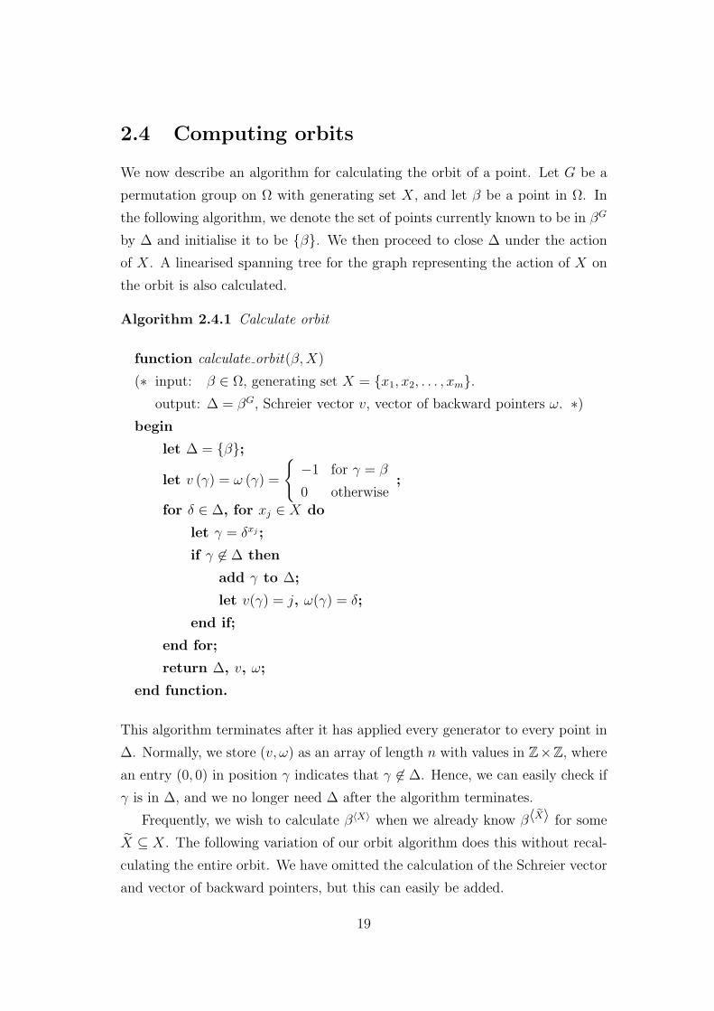
2.4 Computing orbits

We now describe an algorithm for calculating the orbit of a point. Let G be a

permutation group on Ω with generating set X, and let β be a point in Ω. In

the following algorithm, we denote the set of points currently known to be in βG

by ∆ and initialise it to be β. We then proceed to close ∆ under the action

of X. A linearised spanning tree for the graph representing the action of X on

the orbit is also calculated.

Algorithm 2.4.1 Calculate orbit

function calculate orbit(β, X)

(∗ input: β ∈ Ω, generating set X = x1, x2, . . . , xm.output: ∆ = βG, Schreier vector v, vector of backward pointers ω. ∗)

begin

let ∆ = β;

let v (γ) = ω (γ) =

−1 for γ = β

0 otherwise;

for δ ∈ ∆, for xj ∈ X do

let γ = δxj ;

if γ 6∈ ∆ then

add γ to ∆;

let v(γ) = j, ω(γ) = δ;

end if;

end for;

return ∆, v, ω;

end function.

This algorithm terminates after it has applied every generator to every point in

∆. Normally, we store (v, ω) as an array of length n with values in Z×Z, where

an entry (0, 0) in position γ indicates that γ 6∈ ∆. Hence, we can easily check if

γ is in ∆, and we no longer need ∆ after the algorithm terminates.

Frequently, we wish to calculate β〈X〉 when we already know β〈 eX〉 for some

X ⊆ X. The following variation of our orbit algorithm does this without recal-

culating the entire orbit. We have omitted the calculation of the Schreier vector

and vector of backward pointers, but this can easily be added.

19

Algorithm 2.4.2 Extend orbit

function extend orbit(β, X, X, ∆)

(∗ input: β ∈ Ω, X ⊆ X ⊆ SΩ, ∆ = β〈 eX〉.output: ∆ = β〈X〉. ∗)

begin

let ∆ = ∆;

for δ ∈ ∆, for x ∈ X do

if δ 6∈ ∆ or x 6∈ X then

let γ = δx;

if γ 6∈ ∆ then

add γ to ∆;

end if;

end if;

end for;

return ∆;

end function.

2.5 Testing group membership

We now consider a method for testing whether a given permutation is an element

of a group. Let G be a permutation group on Ω with base B = [β1, β2, . . . βk] and

strong generating set S. Suppose that we also know the basic orbits and basic

representative functions with respect to this base. An arbitrary permutation g

on Ω is an element of G if and only if we can express it in the form

g = uk(γk) · uk−1(γk−1) · · · · · u1(γ1),

where every γi ∈ ∆(i).

Theorem 2.5.1 Let G be a permutation group on Ω and let β ∈ Ω. Let

u : βG → G be a representative function. If g ∈ G then, for some h ∈ Gβ,

g = h · u (βg) .

Proof:

We have βg = βu(βg), so βg·u(βg)−1= β. Hence, h = g · u(βg)−1 ∈ Gβ. 2

20

This theorem gives us an algorithm for testing whether a permutation is an

element of G. If g is a permutation on Ω with βg1 6∈ ∆(1), then we know that g

is not in G. Otherwise, we can write g = h · u1(βg1), and then g ∈ G if and only

if h ∈ G(2). The problem has now been reduced to testing whether h is in G(2).

Iterating this process, we find that g can be written in the form

g = g · ul−1(γl−1) · ul−2(γl−2) · · · · · u1(γ1),

where β gl 6∈ ∆(l) or l = k + 1. Clearly, g is in G if and only if g = e. This

algorithm, called stripping with respect to B, is presented more formally below.

Notice that g and l are uniquely determined by g; we call g the residue and l

the drop-out level from stripping g.

Algorithm 2.5.1 Stripping permutations

function strip(g,B,∆, u)

(∗ input: g ∈ G, base B = [β1, β2, . . . , βk] with corresponding ∆, u.

output: residue g and drop-out level l. ∗)begin

let g = g;

for l = 1 to k do

if β gl 6∈ ∆(l) then

return g, l;

else

let g = g · (ul(βgl ))

−1;

end if;

end for;

return g, k + 1;

end function.

This algorithm also plays an important role in Chapter 3, where it is used to

decide if a particular element of a group should be used as a strong generator.

21

2.6 Representing group elements

We now discuss representations for the elements of a group described by a base

and strong generating set. These representations are more memory efficient than

storing a permutation, and they help us to generate random group elements and

list the elements without repetition.

Let G be a permutation group on Ω, with base B = [β1, β2, . . . , βk]. Suppose

we have an element g of G. We can strip it and write it in the form

g = uk(γk) · uk−1(γk−1) · · · · · u1(γ1),

where each γi ∈ ∆(i). The sequence [γ1, γ2, . . . , γk] could then be used to repre-

sent g. This is efficient in terms of memory usage, but two elements stored in

this form must both be converted to permutations before their product can be

calculated. Note that we can generate a random group element by choosing a

random point γi from each ∆(i) and calculating uk(γk) · uk−1(γk−1) · · · · · u1(γ1).

We now present an alternative representation which has the same memory

requirements but is easier to work with.

Definition 2.6.1 The base image of g ∈ G with respect to the base B is

Bg = [βg1 , β

g2 , . . . , β

gk ] .

The following theorem shows that base images are indeed a faithful representa-

tion of the group elements.

Theorem 2.6.1 If the permutation group G has a base B, then the function

g 7→ Bg is one-to-one on G.

Proof:

Suppose g and h are elements of G with Bg = Bh, then[βg·h−1

1 , βg·h−1

2 , . . . , βg·h−1

k

]= [β1, β2, . . . , βk] .

Hence g · h−1 ∈ Gβ1,β2,...,βk= 1, and so g = h. 2

If g and h are in G and [α1, α2, . . . , αk] is the base image of g, then the base

image of g ·h is simply[αh

1 , αh2 , . . . , α

hk

]. Hence, to multiply two elements stored

as base images, it is only necessary to convert one of them into a permutation.

It is easy to convert a permutation to its base image; the following algorithm

performs the converse.

22

Algorithm 2.6.1 Convert from base image to permutation

function base image to permutation(A, u)

(∗ input: base image A = [α1, α2, . . . , αk], basic representative functions u.

output: the group element g corresponding to A. ∗)begin

let g = e;

for i = 1 to k do

let g = ui(αi) · g;for j = i + 1 to k do

let αj = αui(αi)

−1

j ;

end for;

end for;

return g;

end function.

Finally, we consider the problem of listing all the elements of a group without

repetition. We can easily enumerate all the sequences [γ1, γ2, . . . , γk] with each

γi in ∆(i) and calculate the products of the form

uk(γk) · uk−1(γk−1) · · · · · u1(γ1).

However, this involves many permutation multiplications, and so is time con-

suming. Often it suffices to enumerate all the base images of the elements of G.

If g = uk(γk) · uk−1(γk−1) · · · · · u1(γ1) is an element of G, then

βgi = β

ui(γi)·ui−1(γi−1)· ··· ·u1(γ1)i ;

this follows immediately from the fact that uj(γj) ∈ G(j) fixes β1, β2, . . . , βj−1.

Given our list of sequences [γ1, γ2, . . . , γk], we can use this observation to enu-

merate the base images. Note that this method involves calculating images of

points rather than multiplying permutations.

The ability to list the base images allows us to carry out a backtrack search.

This technique can be used to construct a BSGS for a subgroup of G consisting

of all the elements satisfying a certain property. Examples of such subgroups

include centralisers, normalisers, set stabilisers and intersections. A detailed

23

discussion of this method can be found in Butler (1982). A backtrack search

can often be facilitated by choosing a base with certain properties. Sims (1971)

described an effective method for finding a strong generating set with respect to

a given base, provided we already have some base and strong generating set for

the group.

24

Chapter 3

The Schreier-Sims algorithm

In Chapter 2 we considered the use of a base and strong generating set as

a computationally efficient representation for a permutation group. We now

discuss several algorithms which construct such a representation for a group

given by generating permutations. These are all variations of the Schreier-Sims

algorithm described in Section 3.2.

3.1 Partial BSGS and Schreier’s lemma

We use the following definitions and notation throughout this chapter. Let G be

a permutation group on Ω with a generating set X. Suppose B = [β1, β2, . . . , βk]

is a sequence of points in Ω and S is a subset of G. We call B a partial base and S

a partial strong generating set if S contains X and is closed under inversion, and

no element of S fixes every point in B. An ordinary base and strong generating

set is called complete if there is any chance of confusion. Note that k is used to

denote the length of both partial and complete bases. Let i = 1, 2, . . . , k and

define G(i) = Gβ1,β2,...,βi−1and S(i) = S ∩ G(i). In addition, write H(i) =

⟨S(i)

⟩and ∆(i) = βH(i)

i . We now have

G = G(1) ≥ G(2) ≥ · · · ≥ G(k) ≥ G(k+1),

G = H(1) ≥ H(2) ≥ · · · ≥ H(k) ≥ H(k+1) = 1,

G(i+1) = G(i)βi≥ H(i)

βi≥ H(i+1).

A partial basic representative function ui : ∆(i) → H(i) has the property that

βui(γ)i = γ and ui(βi) = e. These functions can be represented by a Schreier

25

structure as shown in Section 2.3, and U (i) = ui(∆(i)) is a set of coset repre-

sentatives for H(i)βi

in H(i). Finally, we write ∆ =[∆(1), ∆(2), . . . , ∆(k)

]and

u = [u1, u2, . . . , uk].

If we have a subset S of G and a sequence B of points, we can use the

following algorithm to extend them to a partial base and strong generating set.

In particular, we can find a partial BSGS for a group given by a generating set

by calling this procedure with B = [ ] and S = ∅.

Algorithm 3.1.1 Find partial BSGS

procedure partial BSGS (var B,var S, X)

(∗ input: S ⊆ G, sequence B of points, generating set X.

output: partial BSGS B and S. ∗)begin

let S = (S ∪ X)\e;let T = S;

for s ∈ T do

if Bs = B then

find a point β not fixed by s;

add β to B;

end if;

if s2 6= e then

add s−1 to S;

end if;

end for;

end procedure.

If Ω = 1, 2, . . . , n, then a point not fixed by a permutation is found by simply

considering each point in turn. With matrix groups, we use the method described

in Section 4.3.

The following theorem, presented in Leon (1980b), is used to verify the cor-

rectness of several of the algorithms in this chapter.

26

Theorem 3.1.1 Suppose G has a partial base B and partial strong generating

set S. Then the following are equivalent:

(i) B is a base and S is a strong generating set.

(ii) H(i+1) = G(i+1), for i = 1, 2, . . . , k.

(iii) H(i)βi

= H(i+1), for i = 1, 2, . . . , k.

(iv)∣∣H(i) : H(i+1)

∣∣ =∣∣∆(i)

∣∣, for i = 1, 2, . . . , k.

Proof:

By definition, (i) is equivalent to (ii). From (ii) we can deduce

H(i)βi

= G(i)βi

= G(i+1) = H(i+1),

so we have (iii). Conversely, if (iii) is true and G(j) = H(j), then

G(j+1) = G(j)βj

= H(j)βj

= H(j+1);

so, by induction on j, (iii) implies (ii). Finally, (iii) is equivalent to (iv) since

H(i+1) ⊆ H(i)βi

and∣∣H(i) : H(i)

βi

∣∣ =∣∣∆(i)

∣∣. 2

A key component of the Schreier-Sims algorithm is Schreier’s lemma, which

allows us to write down a generating set for the stabiliser of a point. Our proof

follows that of Hall, Jr. (1959).

Theorem 3.1.2 Suppose G is a group with generating set X, and H is a sub-

group of G. If U is a set of coset representatives for H in G, and the function

t : G → U maps an element g of G to the representative of H · g, then a

generating set for H is given byu · x · t(u · x)−1 : u ∈ U, x ∈ X

.

Proof:

Every element h of H can be written in the form y1 · y2 · · · · · yl, where each

yi, or its inverse, is in X. Let ui = t(y1 · y2 · · · · · yi), for i = 0, 1, . . . , l. Then

u0 = t(e) = e and ul = t(h) = e, so

h = u0 · h · u−1l = (u0 · y1 · u−1

1 ) · (u1 · y2 · u−12 ) · · · · · (ul−1 · yl · u−1

l ).

27

Consider ui−1 · yi ·ui, for i = 1, 2, . . . , l. Now ui = t(y1 · y2 · · · · · yi) = t(ui−1 · yi),

since H · y1 · y2 · · · · · yi = H · ui−1 · yi. Let u = ui−1 ∈ U and y = yi; we can

now write

ui−1 · yi · u−1i = u · y · t(u · y)−1.

This has the desired form if y ∈ X; otherwise, let y = x−1 for some x ∈ X and

let v = t(u · x−1) ∈ U . Since H · v · x = H · u · x−1 · x, we have t(v · x) = u, and

so the inverse of u · y · t(u · y)−1 can be written

t(u · x−1) · x · u−1 = v · x · t(v · x)−1,

which has the desired form. The result now follows. 2

The generators of H given by this theorem are called Schreier generators.

Suppose that G is a permutation group on Ω and H = Gβ for some β ∈ Ω.

Let u : βG → G be a representative function for Gβ in G. If we take our set of

coset representatives to be U = u (∆), then, by Theorem 2.3.1, t(g) = u(βg), for

all g in G. Hence

t(u(α) · x) = u(βu(α)·x) = u(αx),

for all α ∈ βG, and so the set of Schreier generators for Gβ isu(α) · x · u(αx)−1 : α ∈ βG, x ∈ X

.

This immediately suggests an algorithm for finding a base and strong gen-

erating set. If G has a partial base B = [β1, β2, . . . , βk] and a partial strong

generating set S, then we can find Schreier generators for each G(i+1) by induc-

tion on i. When the algorithm terminates, H(i+1) = G(i+1) for i = 1, 2, . . . , k.

Hence, if we ensure that B, S remains a partial BSGS, then, by Theorem 3.1.1,

we have a complete BSGS. This is presented more formally as Algorithm 3.1.2.

In Hall, Jr. (1959), it is shown that |G : H| − 1 of the Schreier generators

for H are the identity; so the number of non-trivial generators is

1 + |G : H| (|X| − 1) ,

if we ignore the possibility of repetitions among them. Hence, by induction, the

set of Schreier generators for G(i) could be as large as

1 +∣∣∆(1)

∣∣ · ∣∣∆(2)∣∣ · · · ∣∣∆(i)

∣∣ (|X| − 1) .

28

In the next section we consider another algorithm based on Schreier’s lemma,

which constructs a much smaller strong generating set.

Algorithm 3.1.2 Application of Schreier’s Lemma

begin

let X be a generating set of G;

find a partial base B and strong generating set S;

for βi ∈ B do

Schreier(B, S, i);

end for;

end.

procedure Schreier(var B,var S, i)

(∗ input: partial BSGS B = [β1, β2, . . . , βk] and S

such that G(j+1) = H(j+1) for j = 1, 2, . . . , i− 1.

output: extended partial BSGS B = [β1, β2, . . . , βk′ ] and S

such that G(j+1) = H(j+1) for j = 1, 2, . . . , i. ∗)begin

calculate ∆(i) and ui;

let T = S(i);

for α ∈ ∆(i), for s ∈ T do

let g = ui(α) · s · ui(αs)−1;

if g 6= e then

add g and g−1 to S;

if B is fixed by g then

add to B some point not fixed by g;

end if;

end if;

end for;

end procedure.

29

3.2 The Schreier-Sims algorithm

The Schreier-Sims algorithm was first described in Sims (1970), where he dis-

cusses computational methods for determining primitive permutation groups.

This description did not explicitly define the concept of a base and strong gen-

erating set; instead the base was always taken to be [1, 2, . . . , n] and generators

for each stabiliser were considered separately, rather than as a single strong

generating set.

Suppose we have a partial base B and partial strong generating set S, which

we wish to extend to a complete BSGS. Before we add a new Schreier generator

to S, we would like to test whether it is already redundant. We say that level i

of the subgroup chain is complete if every Schreier generator of H(i)βi

has been

included in S or shown to be redundant. Recall that the Schreier generators of

H(i)βi

are elements of the form

ui(α) · s · ui(αs)−1,

for α ∈ ∆(i) = βH(i)

i and s ∈ S(i). If level i is complete, then

H(i)βi

= H(i+1);

so, by Theorem 3.1.1, if every level of the chain is complete, we have a complete

base and strong generating set.

The algorithm in the previous section completes the levels of the chain from

the lowest to the highest. By proceeding from the highest level down, the

Schreier-Sims algorithm provides us with a way of testing potential strong gen-

erators for redundancy. Suppose that we have completed levels i+1, i+2, . . . , k,

where k is the current length of B, then we know that

H(j)βj

= H(j+1)

for j = i+1, i+2, . . . , k. Hence, H(i+1) has a base [βi+1, βi+2, . . . , βk] and strong

generating set S(i+1), by Theorem 3.1.1. We can now use the stripping algorithm

described in Section 2.5 to test for membership of H(i+1).

Suppose g is a new Schreier generator for H(i)βi

. If g is in H(i+1), then it

is redundant as a strong generator, so we need not add it to S. If g is not in

30

H(i+1), then the stripping algorithm returns a residue g 6= e and a drop-out level

l ≥ i + 1. It is clear from the definition of a residue that⟨H(i+1), g

⟩=

⟨H(i+1), g

⟩.

However, adding g to S also extends the groups H(i+2), H(i+3), . . . , H(l−1), while

adding g may not. Once g has been added to S, the levels i + 1, i + 2, . . . , l are

no longer complete, so we continue our computation at level l. If l = k +1, then

g fixes every point in B, so we must add a point not fixed by g to B; we can

now continue at the newly created level k + 1.

In summary, the Schreier-Sims algorithm starts at the highest level of the

chain and attempts to find a Schreier generator whose residue is not the identity.

If successful, it adds the residue to S, and continues at the drop-out level, after

extending B if necessary. Otherwise, it continues at the next lowest level. This

algorithm terminates because there can only be finitely many Schreier generators

for each level of the chain. Algorithm 3.2.1 is a more formal description of it as

a recursive procedure.

We describe one further improvement to the Schreier-Sims algorithm before

we discuss some variations of it. Each time the procedure Schreier-Sims1 is

called at a given level, every possible Schreier generator is stripped, even if it has

been checked during a previous call. The procedure Schreier-Sims2 , presented

as Algorithm 3.2.2, checks each Schreier generator only once. This is achieved

by using the set S, which contains the elements of S which were present the

last time the procedure was called at the current level. We can also use S to

calculate the basic orbits with the Extend orbit algorithm given in Section 2.4.

Note that S and S need not be separate sets, it is only necessary to record which

strong generators have been added since the last call. We can calculate a BSGS

with this procedure by initialising ∆ and u to be empty, and replacing the call

to Schreier-Sims1 in the main part of Algorithm 3.2.1 by

Schreier-Sims2 (B, S, ∅,∆, u, i).

31

Algorithm 3.2.1 Schreier-Sims, version one

begin

let X be a generating set for G;

find a partial base B and strong generating set S;

for i = k down to 1 do

Schreier-Sims1 (B, S, i);

end for;

end.

procedure Schreier-Sims1 (var B,var S, i)

(∗ input: partial BSGS B = [β1, β2, . . . , βk] and S

such that H(j)βj

= H(j+1) for j = i + 1, i + 2, . . . , k.

output: extended partial BSGS B = [β1, β2, . . . , βk′ ] and S

such that H(j)βj

= H(j+1) for j = i, i + 1, . . . , k′. ∗)begin

calculate ∆(i) and ui;

let T = S(i);

for α ∈ ∆(i), for s ∈ T do

let g = ui(α) · s · ui(αs)−1;

strip g wrt H(i+1) to find residue g and drop-out level l;

if g 6= e then

add g and g−1 to S;

if l = k + 1 then

add to B a point not fixed by g;

end if;

for j = l down to i + 1 do

Schreier-Sims1 (B, S, j);

end for;

end if;

end for;

end procedure.

32

Algorithm 3.2.2 Schreier-Sims, version two

procedure Schreier-Sims2 (var B,var S, S,var ∆,var u, i)

(∗ input: partial BSGS B = [β1, β2, . . . , βk] and S

such that H(j)βj

= H(j+1) for j = i + 1, i + 2, . . . , k,

old strong generating set S with corresponding ∆ and u.

output: extended partial BSGS B = [β1, β2, . . . , βk′ ] and S

such that H(j)βj

= H(j+1) for j = i, i + 1, . . . , k′. ∗)begin

let ∆ = ∆(i);

extend ∆(i) and ui;

let T = S(i);

for α ∈ ∆(i), for s ∈ T do

if α 6∈ ∆ or s 6∈ S then

let g = ui(α) · s · ui(αs)−1;

strip g wrt H(i+1) to find residue g and drop-out level l;

if g 6= e then

add g and g−1 to S;

if l = k + 1 then

add to B a point not fixed by g;

end if;

for j = l down to i + 1 do

Schreier-Sims2 (B, S, S \g, g−1,∆, i);

end for;

end if;

end if;

end for;

end procedure.

33

3.3 The Todd-Coxeter Schreier-Sims algorithm

The most time consuming part of the Schreier-Sims algorithm is stripping the

Schreier generators, because this involves a large number of group multiplica-

tions. We now present a method, based on coset enumeration, which verifies

that we have completed a given level of the chain, without having to strip every

Schreier generator.

At the ith level, the Schreier-Sims algorithm ensures that H(i)βi

= H(i+1),

by showing that all the Schreier generators of H(i)βi

are in H(i+1). However, by

Theorem 3.1.1, it suffices to show that∣∣H(i) : H(i+1)∣∣ =

∣∣∆(i)∣∣ .

If we have a presentation for H(i), then we can calculate this index by the

technique of coset enumeration described in Section 1.3. Relators for H(i) can

be obtained from the process of stripping the Schreier generators. If g is a

Schreier generator for H(i)βi

, then stripping it with respect to H(i+1) provides us

with a relation of the form

g = g · ul−1(γl−1) · ul−2(γl−2) · · · · · ui+1(γi+1),

where l is the drop-out level and g is the residue. If we use the Schreier structure

V described in Section 2.3, then we know each uj(γj) as a word in S(j) ⊆ S(i).

In addition, g is of the form ui(α) · s · ui(αs)−1, for some α ∈ ∆(i) and s ∈ S(i),

so it is also known as a word in S(i). Hence, if g = e, we have a new relator

g · ui+1(γi+1)−1 · · · · · ul−2(γl−2)

−1 · ul−1(γl−1)−1

in the existing elements of S(i); otherwise we add g to S (and, thus, to S(i)), and

we have a relator

g · ui+1(γi+1)−1 · · · · · ul−2(γl−2)

−1 · ul−1(γl−1)−1 · g−1

in the elements of S(i). We denote the set of all relators obtained in this way by

R, and we write R(i) for the set of relators in R which only involve elements of

S(i). Often we find that S(i);R(i) is a presentation for H(i) after only a few

Schreier generators have been stripped at level i. In addition to finding a base

and strong generating set, the Todd-Coxeter Schreier-Sims algorithm constructs

a presentation S;R for our group.

34

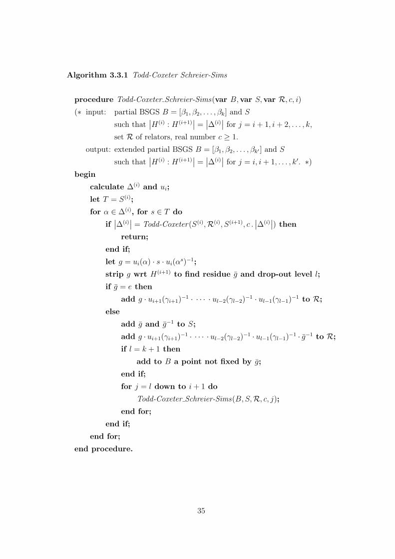
Algorithm 3.3.1 Todd-Coxeter Schreier-Sims

procedure Todd-Coxeter Schreier-Sims(var B,var S,var R, c, i)

(∗ input: partial BSGS B = [β1, β2, . . . , βk] and S

such that∣∣H(i) : H(i+1)

∣∣ =∣∣∆(i)

∣∣ for j = i + 1, i + 2, . . . , k,

set R of relators, real number c ≥ 1.

output: extended partial BSGS B = [β1, β2, . . . , βk′ ] and S

such that∣∣H(i) : H(i+1)

∣∣ =∣∣∆(i)

∣∣ for j = i, i + 1, . . . , k′. ∗)begin

calculate ∆(i) and ui;

let T = S(i);

for α ∈ ∆(i), for s ∈ T do

if∣∣∆(i)

∣∣ = Todd-Coxeter(S(i),R(i), S(i+1), c .∣∣∆(i)

∣∣) then

return;

end if;

let g = ui(α) · s · ui(αs)−1;

strip g wrt H(i+1) to find residue g and drop-out level l;

if g = e then

add g · ui+1(γi+1)−1 · · · · · ul−2(γl−2)

−1 · ul−1(γl−1)−1 to R;

else

add g and g−1 to S;

add g · ui+1(γi+1)−1 · · · · · ul−2(γl−2)

−1 · ul−1(γl−1)−1 · g−1 to R;

if l = k + 1 then

add to B a point not fixed by g;

end if;

for j = l down to i + 1 do

Todd-Coxeter Schreier-Sims(B, S,R, c, j);

end for;

end if;

end for;

end procedure.

35

Algorithm 3.3.1 plays the same role as the procedure Schreier-Sims1 . We

have not incorporated the improvements of Schreier-Sims2 , but these could

easily be added. The function Todd-Coxeter(X,R,S, M) enumerates cosets, as

described in Section 1.3, until either the coset table closes or the number of

cosets exceeds M . It returns the final size of the coset table. The real number

c determines how large we let our coset tables become before we try to find a

new relator, it is normally taken to be about 1.1.

The performance of the Todd-Coxeter Schreier-Sims algorithm is largely de-

pendent on the particular method of coset enumeration used, as is discussed in

Leon (1980b). Rather than recalculating our coset tables, we store one coset ta-

ble for each level of the chain which we modify each time Todd-Coxeter is called

at that level. This technique is called interruptible coset enumeration. Since we

store a number of coset tables, the Todd-Coxeter Schreier-Sims algorithm uses

more memory than the Schreier-Sims algorithm. This may make the algorithm

impractical for groups of large degree.

3.4 The random Schreier-Sims algorithm

The random Schreier-Sims algorithm was first described by Leon (1980b) for use

with the Todd-Coxeter Schreier-Sims algorithm (see Section 3.6). The use of

Schreier generators generally results in an unnecessarily large strong generating

set. The random Schreier-Sims algorithm avoids this problem by using random

elements of the group; we discuss the generation of random group elements

in Section 5.1. This method usually produces a complete BSGS very rapidly,

but we have no way of knowing when it is complete. We decide to terminate

the algorithm when some predetermined condition becomes true. We want this

stopping condition to become true within a reasonable amount of time, while

maximising our chances of finding a complete BSGS. The most common stopping

conditions are discussed in Section 5.2.

During the execution of the random Schreier-Sims algorithm, we cannot be

sure that we have a base and strong generating set for some non-trivial subgroup

of G. However, if we apply the stripping algorithm given in Section 2.5 with

respect to a partial BSGS, it tests for membership of the set

U (k) · U (k−1) · · · · · U (1),

36

where U (i) = ui(∆(i)) is a set of coset representatives for H(i)

βiin H(i). Clearly,

if a random element is in this set, then it is redundant as a strong generator,

otherwise we add the residue of this stripping process to S.

Algorithm 3.4.1 Random Schreier-Sims

begin

let X be a generating set of G;

find a partial base B and strong generating set S;

while stopping condition = false do

let g be a random element of G;

let g be the residue of stripping g wrt B and S;

if g 6= e then

add g and g−1 to S;

if Bg = B then

add to B a point not fixed by g;

end if;

end if;

end while;

end.

In Section 3.6, we briefly discuss methods for verifying that the probable

base and strong generating set produced by this algorithm is complete.

3.5 The extending Schreier-Sims algorithm

The variations of the Schreier-Sims algorithm described so far calculate a BSGS

for a group given by a generating set. We now describe the extending Schreier-

Sims algorithm, which was first implemented by Butler (1979), following a sug-

gestion by Richardson. Assume we have a permutation group H on Ω, and a

permutation g which is not in H. Suppose we also have a base B and strong

generating set S for H. We wish to extend B and S to form a base and strong

generating set for 〈H, g〉. Our algorithm uses the procedure Schreier-Sims2 to

perform this calculation efficiently.

37

Algorithm 3.5.1 Extending Schreier-Sims

begin

let B and S be a BSGS for H;

calculate ∆ and u;

let g be a permutation not in H;

strip g wrt H to find residue g and drop-out level l;

add g and g−1 to S;

if l = k + 1 then

add to B a point not fixed by g;

end if;

for i = l down to 1 do

Schreier-Sims2 (B, S, S\g, g−1,∆, u, i);

end for;

end.

The applications of this algorithm include computing normal closures, com-

mutator subgroups, derived series, and lower and upper central series (see Butler

& Cannon (1982)). In all of these applications, we are working entirely within a

larger group G; that is, H ≤ G and g ∈ G. Frequently, we also know a base C

for G, and so the elements of G can be represented as base images rather than

permutations. This is most useful for stripping Schreier generators.

Algorithm 3.5.2 strips an element of G with respect to the base B for the

subgroup H. It represents the element as an image of the base C. This is faster

than the stripping algorithm in Section 2.5, because a base image can be calcu-

lated more rapidly than a product of two permutations. The residue is returned

as a base image A, and also as a word in S ∪ g (since we have each ui(α) as a

word in S). If A = C, then the residue is trivial; otherwise we can calculate it as

a permutation by evaluating the word. Most of the Schreier generators which are

stripped by the extending Schreier-Sims algorithm have trivial residues, so this

method can lead to significant improvements in the efficiency of the algorithm.

The known base stripping algorithm can also be used with the other variations

of the Schreier-Sims algorithm, if we already know a base for the group which

we are considering. The random Schreier-Sims algorithm is particularly effective

38

when a BSGS is known, because we can also use it to generate random elements,

as described in Section 2.6.

Algorithm 3.5.2 Known base stripping

function strip(g,B,∆, u, C)

(∗ input: g ∈ G, base B with corresponding ∆ and u

for the group H, base C for G.

output: residue g as a word and base image A, drop-out level l ∗)begin

let A = Cg;

let g = g as a word;

for l = 1 to k do

let α = β gl ;

if α 6∈ ∆(l) then

return g, A, l;

else

let g = g · (ul(α))−1 as a word;

let A = Aul(α)−1;

end if;

end for;

return g, A, k + 1;

end function.

3.6 Choice of algorithm

We conclude this chapter with a brief discussion on which variation of the

Schreier-Sims algorithm is most effective for a particular group; a more de-

tailed discussion can be found in Cannon & Havas (1992). If we wish to find a

BSGS for a group of degree under 100, the standard Schreier-Sims algorithm is

generally the fastest method. If the degree exceeds about 300, it is more efficient

to construct a probable BSGS with the random Schreier-Sims algorithm, and

then apply an algorithm to verify that it is complete, or show that it is not.

The Todd-Coxeter Schreier-Sims algorithm is an effective verification algorithm

39

for groups having degrees in the low thousands, and it completes the probable

BSGS if necessary. If our group has higher degree, the Brownie-Cannon-Sims

verification algorithm, which is discussed in Bosma & Cannon (1992), is gen-

erally more efficient. In recent years significant progress has been made in the

construction of bases and strong generating sets for groups of degree up to about

10 million. This is achieved by modifying these algorithms to use less memory;

see, for example, Linton (1989).

If we know more about the group than just a generating set, we can often

construct a BSGS more efficiently. One example of this is the extending Schreier-

Sims algorithm. Another is described in Section 5.2, where we see that if the

order of the group is known in advance, then the random Schreier-Sims algorithm

can be used to construct a complete BSGS.

40

Chapter 4

The random Schreier-Sims

algorithm for matrices

The algorithms described in Chapter 3 construct a base and strong generating

set for a permutation group, which can then be used to investigate the group

structure. We wish to make similar investigations into the structure of matrix

groups over finite fields. Many of the algorithms which have been developed for

matrix group computations are modifications of permutation group algorithms.

In this chapter, we first describe the theory required to adapt permutation

group algorithms to work for matrix groups. Next, we consider data structures

for orbits and representative functions of matrix groups. Finally, we describe an

implementation of the random Schreier-Sims algorithm and discuss the matrix

groups which were used to investigate the performance of this implementation.

In Chapter 5 we consider further implementation issues, and report on some

new methods for improving the range of application of the algorithm for matrix

groups.

4.1 Conversion to matrix groups

Let q = pm be a power of a prime p and let GF (q) be the unique field with q

elements. The set of invertible n× n matrices over GF (q) is denoted by GL(n, q)

and forms a group under matrix multiplication. The following definition is

fundamental to the modification of permutation group algorithms for subgroups

of GL(n, q).

41

Definition 4.1.1 Let G be a group and let SΩ be the group of all permutations

on an arbitrary finite set Ω. An action of G on Ω is a homomorphism from G

to SΩ.

A group action is faithful if it is one-to-one. A faithful action of G on Ω is an

isomorphism between G and a subgroup of SΩ.

There is, of course, a natural action of a matrix group G ≤ GL(n, q) on the

underlying vector space. Let V (n, q) be the n-dimensional space of row vectors

over the field GF (q). We define the action of A ∈ G on v ∈ V (n, q) by vA = vA.

This action is clearly faithful, so G can be considered to be a permutation group

on V (n, q).

We can now apply permutation group algorithms to matrix groups. However,

the number of vectors in V (n, q) is qn, which grows exponentially with n. This

means that the basic orbits can be very large; with simple groups in particular,

the first basic index is often the order of the group. This is demonstrated by the

results in Table 4.1, where the first base point is a vector chosen by the algorithm

outlined in Section 4.3. If we wish to investigate matrix groups using the random

Schreier-Sims algorithm, we must find base points with smaller orbits.

Group n q |∆(1)| |G(2)|A8 28 11 20160 1A8 64 11 20160 1M11 55 7 3960 2M11 44 2 7920 1M12 120 17 95040 1M22 21 7 443520 1M22 34 2 18480 48J1 7 11 14630 12J1 27 11 87780 2J2 42 3 604800 22.J2 36 3 1209600 12.J2 42 3 60480 24.J2 12 3 403200 6U4(2) 58 5 25920 1A5 ×A5 25 7 3600 1

Table 4.1: Lengths of first basic indices

42

One technique for finding smaller basic orbits is to consider the action of G

on a set other than V (n, q); for example, the set of subspaces of V (n, q). Often

this means using an action which is not faithful, in which case we also take base

points in V (n, q), or else we only construct a BSGS for the quotient of G by

the kernel of the action. In Section 5.3, we consider actions of matrix groups on

several different sets. A second method, discussed in Section 5.4, reduces the

orbit sizes by choosing points which we expect a priori to have small orbits.

4.2 Orbits and Schreier structures

In this section, we discuss the storage of basic orbits and representative functions

for matrix groups. Suppose we have a group G with a base [β1, β2, . . . , βk] and

strong generating set S. Recall from Section 2.3 that we want a data structure for

the basic orbits ∆ =[∆(1), ∆(2), . . . , ∆(k)

], together with a Schreier structure

for the basic representative functions u = [u1, u2, . . . , uk]. With permutation

groups on Ω = 1, 2, . . . , n, a possible Schreier structure is the k × n array

U (i, γ) =

ui(γ) for γ ∈ ∆(i)

0 otherwise.

An alternative is the k × n array

V (i, γ) =

(vi(γ), ωi(γ)) for γ ∈ ∆(i)

(0, 0) otherwise,

where (vi, ωi) is a linearised spanning tree of the graph representing the action

of S(i) on ∆(i). If we use either of these Schreier structures, we do not need to

store the basic orbits separately, since α ∈ ∆(i) if and only if the (i, α) position

of the array is non-zero.

These Schreier structures rely critically on the fact that the point set has a

predetermined size and a natural linear ordering. If G is a matrix group, we can

use points of many different types and it is impractical to impose an order on

the entire point set. Instead, we choose a positive integer N , which we hope will

be an upper bound on the lengths of the basic orbits of G. We can now store the

basic orbits as a k ×N array O where, for i = 1, 2, . . . , k and m = 1, 2, . . . , N ,

O(i, m) ∈ ∆(i) ∪ 0;

43

and, for each α ∈ ∆(i), there is exactly one integer m such that O(i, m) = α.

Now, for each i = 1, 2, . . . , k, this array provides us with a one-to-one correspon-

dence between ∆(i) and some subset of 1, 2, . . . , N, so we can use the natural

ordering on Z to impose an ordering on each basic orbit.

We can now define Schreier structures for matrix groups which are analogous

to U and V . Our first Schreier structure is the k×N array with values in G ∪ 0defined by

U ′(i, m) =

ui O(i, m) if O(i, m) 6= 0

0 otherwise;

however, this requires too much memory to be practical for most groups. An-

other, more memory efficient, Schreier structure is the k ×N array with values

in Z× Z given by

V ′(i, m) =

(vi O(i, m), m′) if O(i, m) 6= 0

(0, 0) otherwise,

where m′ is the unique integer such that O(i, m′) = ωi O(i, m).

When the basic orbits and representative functions are stored in this way, we

must make frequent searches for particular points in each row of the array O.

Probably the most efficient search method available is a hash search algorithm,

several varieties of which are described in detail in Knuth (1973). Here we briefly

describe the linear probe hash search algorithm. First, we must choose a hash

function

h : Ω→ 1, 2, . . . , N,

where Ω contains all the different points we might use. If we wish to add α

to ∆(i), we store it as O(i, h(α)), unless that entry in the array already holds

a point, in which case we store it in the next free position in the ith row of

O. We can now test a point α for membership of ∆(i) by searching the ith row

from position h(α), rather than from the beginning. This is an effective search

algorithm, provided we choose a hash function which can be calculated rapidly

and whose values are roughly uniformly distributed over the range 1, 2, . . . , N . If

a row of the arrayO is almost full, the search algorithm slows down considerably;

hence, N should be at least 4/3 of the length of the longest basic orbit.

44

4.3 Implementations

The first matrix group implementation of the random Schreier-Sims algorithm

was developed by Butler (1976; 1979), who also implemented the other algo-

rithms described in Chapter 3. He chose his points to be one-dimensional sub-

spaces and vectors, as described in Section 5.3. The basic orbits and represen-

tative functions were stored in data structures similar to O and V ′, and a hash

search algorithm was used. He also carried out some preprocessing to find short

orbits. This consisted of choosing a random point and building up its orbit until

it was complete or it exceeded 5000 in length. If its orbit was complete, it was

taken to be the first basic orbit, otherwise the process was repeated.

The random Schreier-Sims algorithm has been implemented for matrix groups

over fields of prime order as part of this project. This implementation is written

in traditional C (Kernighan & Ritchie, 1988). The orbits are stored as an array

O which is searched with the linear probe hashing algorithm, and we use the

Schreier structure V ′. We now present the algorithm used to calculate our hash

function on the vectors in V (n, q).

Algorithm 4.3.1 Hash function

function h(v)

(∗ input: vector v = (v1, v2, . . . , vn).

output: value of the hash function for v. ∗)begin

let hash = 0;

for i = 1 to n do

left shift hash;

let hash = hash xor vi;

end for;

return (hash mod N) + 1;

end function.

We use the bitwise exclusive or operation (xor) on the entries of the vector

because it is usually faster than arithmetical operations. A left shift by m bits,

essentially multiplication by 2m, is used to achieve a roughly uniform distribution

45

of values for the hash function; the value of m used depends on the ratio of n to

the number of bits used to store an entry in our vector. Similar hash functions

can be defined for subspaces and other types of point.

Our implementation uses vectors and subspaces for the base points, as de-

scribed in Section 5.3. It accepts from the user an arbitrary number of points,

which are used as the initial base points. Whenever we find a new strong genera-

tor A which fixes the existing points, a new base point is chosen by the following

algorithm. If A is not scalar, the vector chosen has the property that the one-

dimensional subspace generated by it is also not fixed by A. Note that ei is the

ith standard basis vector; that is, the vector with one as its ith entry and zeros

elsewhere.

Algorithm 4.3.2 Choose new base point

function base point(A)

(∗ input: I 6= A ∈ GL(n, q).

output: v ∈ V (n, q) such that vA 6= v and, if possible, vA 6∈ 〈v〉. ∗)begin

for i = 1 to n, for j = 1 to n do

if i 6= j and Aij 6= 0 then (∗ A not diagonal ∗)return ei;

end if;

end for;

for i = 1 to n, for j = 1 to n do

if i 6= j and Aii 6= Ajj then (∗ A not scalar ∗)return ei + ej;

end if;

end for;

if A11 6= 1 then (∗ A 6= I ∗)return e1;

else

return error;

end if;

end function.

46

4.4 Evaluating performance

We used a variety of matrix groups to investigate the performance of our im-

plementation of the random Schreier-Sims algorithm. These groups are of three

types:

1. soluble groups;

2. almost simple groups;

3. simple groups and related constructions.

The results of these tests are given in the next chapter; for future reference,

we list in this section all the groups mentioned there, together with their or-

ders. If possible, groups are described using the notation of the Atlas (Conway

et al., 1985). Most of the groups were either obtained from the libraries of the

computational algebra systems Cayley and GAP, or were constructed using GAP.

The soluble groups were constructed by calculating the wreath product of a

soluble subgroup of a small general linear group and a p-group. The subgroups

of general linear groups are from the libraries constructed by Short (1992), which

contain all of the soluble subgroups of GL(2, 7), GL(4, 3), GL(5, 3) and GL(6, 2).

The p-groups are subgroups of Spm for some m, constructed following the de-

scription in Hall, Jr. (1959). In Table 4.2 we list the soluble groups used; the

wreath product of the ith member of Short’s GL(n, q) library with a p-subgroup

of Spm is denoted by GL(n, q)–i–pm.

Group n q OrderGL(2, 7)–15–24 32 7 263316

GL(2, 7)–3–33 54 7 281313

GL(4, 3)–1–33 108 3 313527

GL(4, 3)–1–24 64 3 215516

GL(4, 3)–50–33 108 3 2135340

GL(5, 3)–2–33 135 3 2273131127

GL(5, 3)–9–24 80 3 295516

GL(6, 2)–10–24 96 2 231348

GL(6, 2)–21–33 162 2 2273121

GL(6, 2)–33–23 48 2 239324

Table 4.2: Soluble groups

47

Aschbacher’s 1984 classification of the subgroups of GL(n, q) divides them

into nine categories. Various researchers are working on the matrix group “recog-

nition project”, which seeks to construct algorithms which recognise groups in

these categories (see, for example, Neumann & Praeger (1992)). It is expected

that the category of almost simple groups will pose the greatest difficulty.

Definition 4.4.1 Suppose G ≤ GL(n, q) and Z is the subgroup of scalar ma-

trices in G. Then G is almost simple if there is a non abelian simple group T

such that T ≤ G/Z ≤ Aut T .

In private communication, Praeger asked if the random Schreier-Sims algorithm

is particularly effective when applied to almost simple groups. In particular,

she suggested constructing the permutation module of Sm over GF (q), and then

applying the Meataxe to this reducible module. See Holt & Rees (1994) for a

description of the Meataxe. The largest composition factor has dimension m−1,

or m− 2 if q divides m. This factor is isomorphic to Sm and is an almost simple

group with T = Am. The values of m and q which we used are listed in Table 4.3.

m q m q m q

20 5 30 31 57 320 23 35 2 63 5325 17 40 2 65 1130 7 50 53 72 2

Table 4.3: Almost simple groups

Our final collection of test groups contains simple groups (mostly sporadic);

covers, subgroups and other constructions based on simple groups; and also a

couple of miscellaneous examples. The representations listed in Table 4.4 are

obtained from the matrix group libraries of Cayley and GAP, and a number of

other sources. Note that (32 :4×A6)·2 is a maximal subgroup of 3.O’N; the

group GL(5, 3) is represented as a subgroup of GL(20, 3); and φF (2, 9) is the

representation of the quotient of the Fibonacci group, F (2, 9), constructed by

Havas, Richardson & Sterling (1979).

48

Group n q OrderA8 20 11 20,160A8 28 11 20,160A8 64 11 20,160M11 24 3 7920M11 44 2 7920M11 44 7 7920M11 55 7 7920M12 55 7 95,040M12 120 17 95,040M22 21 7 443,5202.M22 34 2 887,040J1 7 11 175,560J1 14 11 175,560J1 27 11 175,5602.J2 36 3 1,209,6002.J2 42 3 1,209,6004.J2 12 3 2,419,2006.J3 18 2 301,397,760U4(2) 58 5 25,920U4(2) 64 2 25,920U4(2) 81 11 25,920(32 :4×A6)·2 18 7 77,760(32 :4×A6)·2 27 7 77,760(32 :4×A6)·2 45 7 77,760Sz (8) 65 29 29,1204.Suz 12 3 1,793,381,990,400A5 ×A5 25 7 3600M11 oM11 55 3 792012

GL(5, 3) 20 3 475,566,474,240φF (2, 9) 19 5 579,833,984,375,000

Table 4.4: Simple groups and related constructions

In the next chapter, we use these groups to investigate several aspects of

the implementation of the random Schreier-Sims algorithm. Most tests were re-

peated 10 times on a Sparc Station 10/51. We give timings in seconds, averaged

over those runs which found a complete BSGS.

49

Chapter 5

Investigating performance

In this chapter, we consider four topics related to the implementation of the

random Schreier-Sims algorithm. Our discussion of methods for generating ran-

dom elements and stopping conditions pertains to both permutation and matrix

group versions of the algorithm. Next, we describe several sets on which ma-

trix groups have a natural action, and discuss which are useful for the random

Schreier-Sims algorithm. Finally, we describe new techniques which significantly

extend the range of application of the random Schreier-Sims algorithm for ma-

trices, by finding particular points which have small orbits.

5.1 Random elements

The generation of random group elements is an important aspect of the random

Schreier-Sims algorithm, for both matrix and permutation groups. If we already

know a base and strong generating set, we can produce uniform random elements

by the method described in Section 2.6. This is useful if we want a smaller strong

generating set or a strong generating set with respect to a different base.

If no BSGS is known, nearly uniform random elements can be generated by

the algorithm described in Babai (1991). However, this algorithm has complexity

O(n10(log q)5) for matrix groups, and no practical implementation of it has yet

been developed. An alternative method presented in Holt & Rees (1992) is more

practical, but is not guaranteed to produce nearly uniform random elements. We

now present a similar method which is used in our implementation of the random

50

Schreier-Sims algorithm. It is based on a GAP program written by Leedham-

Green and O’Brien, as well as a number of suggestions made by Cannon in

personal communication.

Our algorithm for generating random group elements is based on the evalu-

ation of random words in the strong generators. If the random words we choose

are relatively short, we may only produce elements from a small part of the

group. However, both matrix and permutation multiplications involve a large

number of operations, so evaluating long words is time consuming. This problem

is solved by storing some of the evaluated words which we have previously ob-

tained. When we need a new random element, we compute the product of one of

these stored elements with either another stored element or a strong generator.

We multiply by strong generators occasionally to ensure that they all occur in

the random words produced. While this method only requires a single multipli-

cation for each evaluated word, the length of the word grows exponentially.

The algorithm presented below is in two parts: the initialise procedure which

is called once before generating random elements; and the random element func-

tion which then returns a random element. It is controlled by three predeter-

mined parameters:

• num — the number of evaluated words to store;

• len — the length of the words after executing initialise;

• prob — the probability of multiplying by another evaluated word rather

than a strong generator.

The procedure initialise may reset num, so that it is at least as large as the

initial number of strong generators; this allows us to ensure that every strong

generator appears in at least one of the initial words. The other two parameters

remain constant. Evaluated words are stored in the array

w : 0, 1, . . . , num − 1 → G.

The variable current is the position in w of the evaluated word we are currently

considering. Note that in random element we randomly decide whether to pre-

or post-multiply w(current) by the group element x.

51

Algorithm 5.1.1 Random element generation

procedure initialise(S,var w,var num, len)

(∗ input: partial strong generating set S = s0, s1, . . . , sm−1,integers num and len.

output: array w of num evaluated words of length len. ∗)begin

let num = max(num, m);

for current = 0 to num − 1 do

let j1 = current mod m;

(∗ each element of S must occur in at least one word ∗)let j2, j3, . . . , jlen be random integers in 0, 1, . . . ,m− 1;let w(current) = sj1 · sj2 · · · · · sjlen

;

end for;

end procedure.

function random element(S,var w, num, prob)

(∗ input: partial strong generating set S = s0, s1, . . . , sm−1,array w of num evaluated words, probability prob.

output: return random element. ∗)begin

let current = (current + 1) mod num;

let r be a random real number in [0, 1];

if r ≤ prob then

let i be a random integer in 0, 1, . . . , num − 1;let x = w(i);

else

let i be a random integer in 0, 1, . . . ,m− 1;let x = si;

end if;

let w(current) = w(current) · x or x · w(current);

return w(current);

end function.

52

In Table 5.1, we present results demonstrating the impact of varying the three

parameters on the performance of our implementation of the random Schreier-

Sims algorithm. The second stopping condition described in Section 5.2 was

used with C = 10. The column labelled “/10” contains the number of runs out

of 10 which gave a complete BSGS. Tests were carried out on a soluble group

with 14 generators and a “related construction” with 3 generators. These results

indicate that the random Schreier-Sims algorithm is more reliable if we increase

the initial lengths of the words; this makes the random elements more uniform.

However, the time taken also increases.

Group n q num len prob Time /10GL(6, 2)–10–24 96 2 14 2 0.75 2720 5

14 10 0.75 2839 914 20 0.75 3099 1028 2 0.75 2598 414 2 0.25 3370 214 2 0.99 2665 5

(32 :4×A6)·2 45 7 5 2 0.75 305 45 10 0.75 319 105 20 0.75 323 10

10 2 0.75 312 75 2 0.25 309 95 2 0.99 312 6

Table 5.1: Investigating random element generation

The first implementation of the random Schreier-Sims algorithm by Leon

(1980a) stored a single evaluated word, which was initialised to be a generator

and multiplied by another generator to produce each new random element. The

algorithm described by Holt & Rees (1992) stored about 10 evaluated words

whose initial length was around 30; they were producing random matrices for

a group recognition algorithm in which uniformness was more critical than it is

with the random Schreier-Sims algorithm. Following a suggestion by Cannon,

we use the following values as our default:

num = 5, len = 2, prob = 0.75;

observe from Table 5.1 that these are not necessarily optimal.

53

5.2 Stopping conditions

The choice of stopping condition is a very important aspect of the random

Schreier-Sims algorithm. Recall, from Section 3.4, that to ensure that the al-

gorithm terminates, we stop testing new random elements when some prede-

termined condition becomes true. If we know the order of the group, we can

choose a stopping condition which makes the algorithm deterministic. Otherwise

we need a stopping condition which maximises the probability that a complete

BSGS will be constructed, while minimising the number of random elements

considered.

The three most common stopping conditions are:

1. R random elements have been considered;

2. C consecutive random elements have all stripped to the identity;

3. the product of the lengths of the partial basic orbits has reached L;

where R, C and L are positive integers chosen in advance. The first condition

allows us to calculate an upper bound on the running time of the algorithm,

provided we have a bound on the lengths of the basic orbits. The second allows

us to estimate the probability that the partial BSGS produced is complete, as

shown below. If the order of the group is known in advance, we set L to be the

order and use the third stopping condition.

Combinations of these conditions can also be used. The implementation of

the random Schreier-Sims algorithm in Cayley asks for numbers R and C and

then terminates when either (1) or (2) is true. If we have a lower bound L on

the group order, then we can choose an integer C and stop when both (2) and

(3) are true. Similarly, if we have an upper bound L, we choose C and stop

when either (2) or (3) is true.

The following result, presented in Leon (1980b), allows us to estimate the

probability that our partial BSGS is complete when the second stopping condi-

tion is used.

54

Theorem 5.2.1 If B is a partial base and S is a partial strong generating set

for G, then∣∣U (k) · U (k−1) · · · · · U (1)

∣∣ =∣∣∆(k)

∣∣ .∣∣∆(k−1)

∣∣ . . . . .∣∣∆(1)

∣∣ divides |G|.

Proof:

It is easily seen that∣∣U (k) · U (k−1) · · · · · U (1)∣∣ =

∣∣∆(k)∣∣ .

∣∣∆(k−1)∣∣ . . . . .

∣∣∆(1)∣∣ .

Since∣∣∆(i)

∣∣ =∣∣∣H(i) : H

(i)βi

∣∣∣, we have

|G| =k∏

i=1

∣∣H(i) : H(i+1)∣∣ .

∣∣H(k+1)∣∣

=∣∣H(k+1)

∣∣ .k∏

i=1

∣∣∣H(i) : H(i)βi

∣∣∣ .∣∣∣H(i)

βi: H(i+1)

∣∣∣=

∣∣H(k+1)∣∣ .

k∏i=1

∣∣∆(i)∣∣ .

∣∣∣H(i)βi

: H(i+1)∣∣∣ ,

so∣∣∆(k)

∣∣ .∣∣∆(k−1)

∣∣ . . . . .∣∣∆(1)

∣∣ divides |G|. 2

If U (k) · U (k−1) · · · · · U (1) is not the entire group, then it contains at most half

of the elements of G. Suppose g ∈ G has residue g with respect to our partial

BSGS. Now g = e if and only if

g ∈ U (k) · U (k−1) · · · · · U (1);

so, if g is a uniform random element of G and our partial BSGS is not complete,

there is a probability of at least 1/2 that g 6= e. Hence, if C consecutive random

elements strip to the identity, the probability that our strong generating set

is still not complete is at most 2−C . Since we are not using uniform random

elements, this calculation is not exact, but it can still be used as a rough guide

in choosing C.

Note that the set U (k) · U (k−1) · · · · · U (1) considered in Theorem 5.2.1 is not

necessarily a subgroup of G, so using a partial BSGS instead of a complete one

can have unpredictable results.

Our implementation was tested with stopping conditions (2) and (3). Ta-

ble 5.2 gives timings for condition (2) with C = 10, 30 or 50, and for condition

(3) with L equal to the order of the group. In addition, the columns labelled

55

Group n q C = 10 C = 30 C = 50 L = |G|time /10 time /10 time /10 time

GL(2, 7)–3–33 54 7 1449 10 1636 10 1767 10 1497GL(4, 3)–1–33 108 3 1970 9 3074 10 4367 10 2007GL(4, 3)–50–33 108 3 24211 10 26167 10 29166 10 22284GL(5, 3)–2–33 135 3 12102 8 16629 10 22310 10 8093GL(5, 3)–9–24 80 3 6550 7 7214 10 7942 10 6469S30 29 7 188 3 224 5 270 9 211S30 29 31 208 2 199 6 239 8 169S50 49 53 1948 1 2824 6 3297 7 3036S57 55 3 5052 2 6131 7 5853 9 6562S63 62 53 8441 1 10418 2 11213 6 10198S65 64 11 — 0 10984 1 13917 4 10061A8 20 11 40 10 40 10 42 10 38A8 28 11 68 10 74 10 76 10 68A8 64 11 319 10 360 10 412 10 313M11 24 3 10 5 14 9 19 10 10M11 44 2 44 10 62 10 84 10 42M11 44 7 47 10 64 10 88 10 45M11 55 7 55 5 103 10 154 10 52M12 55 7 809 10 850 10 902 10 810M12 120 17 15475 10 16127 10 16712 10 15588M22 21 7 666 10 682 10 675 10 6722.M22 34 2 — 0 193 10 222 10 180J1 14 11 140 10 141 10 141 10 141J1 27 11 276 6 283 10 290 10 2812.J2 36 3 6183 10 6252 10 6244 10 62682.J2 42 3 — 0 5108 9 5363 10 51434.J2 12 3 350 1 396 10 394 10 3946.J3 18 2 — 0 453 4 477 8 437U4(2) 58 5 247 10 276 10 348 10 243U4(2) 64 2 80 5 129 10 197 10 49U4(2) 81 11 172 4 339 10 478 10 145(32 :4×A6)·2 18 7 61 6 63 10 64 10 61(32 :4×A6)·2 27 7 122 6 126 10 131 10 122(32 :4×A6)·2 45 7 305 4 324 10 343 10 307Sz (8) 65 29 55 4 111 10 161 10 374.Suz 12 3 — 0 160 6 160 10 154A5 ×A5 25 7 16 10 18 10 20 10 15M11 oM11 55 3 3297 10 3436 10 3790 9 3253GL(5, 3) 20 3 11 10 15 10 18 10 9φF (2, 9) 19 5 14 10 18 10 22 10 12

Table 5.2: Comparison of stopping conditions

56

“/10” contain the number of executions out of ten which yielded a complete

base and strong generating set. These results demonstrate that C = 10 is far

too small for us to have any confidence in the partial BSGS produced, C = 30

is sufficient for most groups, and C = 50 gives us a complete BSGS in almost

every case. When the third stopping condition is used, the random Schreier-

Sims algorithm almost always outperforms the Schreier-Sims and Todd-Coxeter

Schreier-Sims algorithms.

Clearly, considering a larger number of random elements increases the proba-

bility that our BSGS is complete. However, a comparison with Table 5.1 suggests

that a more efficient method of achieving this goal is to generate random ele-

ments which are more uniform. All the timings reported in the next two sections

are for stopping condition (2) with C = 50.

5.3 Point sets

The most natural action of a matrix group is on the underlying vector space,

as we saw in Section 4.1. In this section, we consider several other point sets

for matrix groups and discuss their usefulness for the random Schreier-Sims

algorithm. The properties that make a point set useful for this algorithm include:

• There must be an efficient method for calculating the image of a point

under the action of a matrix.

• It must be easy to determine if two points are identical; ideally, we want

a canonical representation for each point.

• The memory requirements of a point should be comparable to those of a

vector.

• The action of the group on the point set should produce small orbits which

can be found easily.

Suppose G ≤ GL(n, q). One of the most obvious types of point is a set

W ⊆ V (n, q) with the action of A ∈ G defined by

WA = wA : w ∈ W .

57

Such sets occupy more memory than single vectors and their images take longer

to calculate. While they may have shorter orbits, this cannot compensate for

the increased memory required for each point. If w ∈ W , then clearly every

vector in wG is contained in at least one of the sets in WG; hence, to store the

orbit of W , we must store at least as many vectors as are contained in the union

of the orbits of the elements of W . A similar argument applies for ordered tuples

of vectors.

Subspaces of V (n, q) are more useful than arbitrary sets. We need only store

a basis, and we can calculate the action of a matrix by considering its action on

each basis vector. The basis can be stored as the rows of a matrix, which is then

row-reduced to produce a canonical representation. An efficient row-reduction

algorithm is necessary if we use multi-dimensional subspaces.

Row-reduction of the matrix of a one-dimensional subspace is simply multi-

plication by a scalar. Hence, one-dimensional subspaces have the same memory

requirements as vectors, and the action of a matrix takes only slightly longer

to calculate. Suppose we have v ∈ V (n, q) whose orbit vG has length M . Now

suppose that, instead of taking our first base point to be v, we take β1 = 〈v〉 and

β2 = v. Then every element of ∆(2) = βGβ12 is of the form λv for some non-zero

λ ∈ GF (q) and it is easily seen thatλ : λv ∈ ∆(2)

is a subgroup of the multiplicative group of GF (q). Hence, the length of ∆(2) is

a divisor d of q − 1 and, instead of having to calculate one orbit of length M ,

we calculate two orbits whose lengths are M/d and d. More generally, we can

precede every vector in our base by the one-dimensional subspace containing it.

This method was first suggested by Butler (1976). It is least effective for smaller

fields, and of no benefit over GF (2).

An arbitrary subspace of dimension higher than one is unlikely to be more

useful than a one-dimensional subspace. However, eigenspaces can be useful,

as we see in the next section. Sets of subspaces offer no improvement over

individual subspaces, by the same argument used for sets of vectors. Other

structures might be useful for particular types of groups, but we restrict our

attention to point sets which are potentially useful for arbitrary matrix groups.

58

We now present some timings for the random Schreier-Sims algorithm using

Butler’s method of alternating one-dimensional subspaces and vectors. We also

list the first ten basic indices. Since the basic indices sometimes vary for different

runs of the algorithm, we present only one example for each group.

The results in Table 5.3 demonstrate that the random Schreier-Sims algo-

rithm is very effective for soluble groups. Although the implementation took a

long time with some of the groups, this is due to the large matrix dimension and

group order, rather than the size of the orbits.

Group n q Time Basic indicesGL(2, 7)–15–24 32 7 149 64 6 8 6 16 6 8 6 4 6 . . .GL(2, 7)–3–33 54 7 1767 45 2 2 1 6 2 6 2 18 2 . . .GL(4, 3)–1–33 108 3 4367 135 1 15 1 15 1 45 1 15 1 . . .GL(4, 3)–1–24 64 3 540 80 1 10 1 20 1 10 1 40 1 . . .GL(4, 3)–50–33 108 3 29166 216 2 24 2 24 2 3 2 72 2 . . .GL(5, 3)–2–33 135 3 22310 297 2 33 2 33 2 99 2 33 2 . . .GL(5, 3)–9–24 80 3 7942 80 2 4 1 2 1 2 1 10 2 . . .GL(6, 2)–10–24 96 2 4760 144 1 18 1 36 1 18 1 6 1 . . .GL(6, 2)–21–33 162 2 68523 243 1 6 1 27 1 81 1 81 1 . . .GL(6, 2)–33–23 48 2 459 288 1 2 1 36 1 6 1 2 1 . . .

Table 5.3: Soluble groups

The results for almost simple groups, in Table 5.4, demonstrate that these

methods are usually just as effective as for the soluble groups. However, in three

cases, the algorithm failed to complete in a “reasonable” time; this is indicated

by the ∞ symbol.

59

Group n q Time Basic indicesS20 18 5 27 190 2 18 1 17 1 16 1 15 1 . . .S20 19 23 ∞S25 24 17 96 300 2 23 1 22 1 21 1 20 1 . . .S30 29 7 270 435 2 28 1 27 1 26 1 25 1 . . .S30 29 31 239 435 2 28 1 27 1 26 1 25 1 . . .S35 34 2 ∞S40 38 2 ∞S50 49 53 3297 1225 2 48 1 47 1 46 1 45 1 . . .S57 55 3 5853 1596 2 55 1 54 1 53 1 52 1 . . .S63 62 53 11212 1953 2 61 1 60 1 59 1 58 1 . . .S65 64 11 13917 2080 2 63 1 62 1 61 1 60 1 . . .S72 70 2 16799 2556 1 140 1 69 1 68 1 67 1 . . .

Table 5.4: Almost simple groups

The results in Table 5.5 show that, for most of our simple groups and related

constructions, the first basic orbit is very large compared to the other orbits.

60

Group n q Time Basic indicesA8 20 11 42 20160 1A8 28 11 76 20160 1A8 64 11 412 20160 1M11 24 3 19 3960 2M11 44 2 84 7920 1M11 44 7 88 7920 1M11 55 7 154 3960 1 2 1M12 120 17 16712 95040 1M12 55 7 902 95040 1M22 21 7 675 443520 12.M22 34 2 222 18480 1 24 1 2 1J1 7 11 8 7315 2 6 1 2 1J1 14 11 141 175560 1J1 27 11 290 87780 22.J2 36 3 6244 1209600 12.J2 42 3 5363 60480 1 2 14.J2 12 3 394 201600 2 6 16.J3 18 2 477 130815 1 1152 1 2 1U4(2) 58 5 348 25920 1U4(2) 64 2 197 270 3 16 2U4(2) 81 11 478 810 2 16 1(32 :4×A6)·2 18 7 64 25920 3(32 :4×A6)·2 27 7 131 25920 3(32 :4×A6)·2 45 7 343 25920 3Sz (8) 65 29 161 65 7 64 14.Suz 12 3 160 32760 2 1980 2 96 1 36 1 2 1A5 ×A5 25 7 20 3600 1M11 oM11 55 3 3790 1210 2 1100 2 990 2 880 2 110 2 . . .GL(5, 3) 20 3 18 121 2 120 2 117 2 108 2 81 2φF (2, 9) 19 5 22 190 4 5 1 5 1 5 1 5 1 . . .

Table 5.5: Simple groups and related constructions

61

5.4 Eigenvectors and eigenspaces

In the previous section, we considered different point sets on which a matrix

group can act. We now consider the possibility of choosing particular points in

these sets which we expect will have small orbits for some theoretical reason. The

points we choose are eigenvectors and eigenspaces of the generating matrices.

This differs significantly from the technique used by Butler to find small orbits,

which we discussed in Section 4.3.

Definition 5.4.1 Let A be an n × n matrix over GF (q). The characteristic

polynomial of A is

cA(x) = det(xI − A),

where I is the identity matrix. For each irreducible factor g(x) of cA(x), there

is a corresponding eigenspace

v ∈ V (n, q) : v. g(A) = 0.

An eigenvector is a non-zero element of an eigenspace.

Note that this definition differs slightly from the standard one, which only con-

siders linear factors of cA(x). We consider the impact of the following selections

on the performance of the random Schreier-Sims algorithm:

• Let the first base point be an eigenvector of a generator.

• Let the first base point be an eigenvector of more than one generator.

• Let the first base point be an eigenspace of a generator.

• Let several initial base points be eigenvectors of the generators.

Eigenspaces and eigenvectors can be found efficiently for matrices of large di-

mension; in practice, we computed them using GAP.

If g(x) is linear, say g(x) = x−λ, then for any eigenvector v we have vA = λv,

and so the orbit v〈A〉 contains at most q − 1 points. Hence, we expect that the

orbit of v under the action of G will be shorter than the orbit of a vector chosen

by the method of Section 4.3. Suppose now, for example, that g(x) = x2 +x+1,

then we have vA2+A = −v. Since this formula involves addition of matrices as

62

well as multiplication, we have less reason to believe that the eigenvectors will

have small orbits. We take as base points eigenvectors corresponding to factors

whose degree is minimal. If there is more than one such factor, we choose an

eigenvector from an eigenspace of the smallest dimension.

We found a linear factor of a characteristic polynomial for every one of our

simple groups and related constructions. Using a corresponding eigenvector as

the first base point frequently leads to significant improvements in the perfor-

mance of the implementation, as shown in Table 5.6.

Group n q Deg Dim Time |∆(1)|A8 20 11 1 2 9 2880A8 28 11 1 4 19 2880A8 64 11 1 10 153 2880M11 24 3 1 6 10 110M11 44 2 1 12 45 1980M11 44 7 1 12 57 1980M11 55 7 1 13 100 1980M12 55 7 1 18 360 31680M12 120 17 1 40 2868 31680M22 21 7 1 6 228 1108802.M22 34 2 1 20 194 18480J1 7 11 1 1 5 5852J1 14 11 1 2 17 12540J1 27 11 1 3 59 125402.J2 36 3 1 5 389 378002.J2 42 3 1 7 1557 1512004.J2 12 3 1 4 35 126006.J3 18 2 1 6 167 61560U4(2) 58 5 1 14 101 6480U4(2) 64 2 1 16 223 6480U4(2) 81 11 1 21 399 6480(32 :4×A6)·2 18 7 1 2 8 1080(32 :4×A6)·2 27 7 1 3 23 2160(32 :4×A6)·2 45 7 1 2 71 1080Sz (8) 65 29 1 16 331 72804.Suz 12 3 1 6 141 32760A5 ×A5 25 7 1 5 8 720M11 oM11 55 3 1 1 3265 121GL(5, 3) 20 3 1 6 18 121φF (2, 9) 19 5 1 1 23 1

Table 5.6: Using eigenvectors of a generator

63

Using eigenvectors of a single generator guarantees a small orbit under the

action of that matrix, but not the others. Sometimes, a vector is an eigenvector

of more than one generator. The results of using eigenvectors of two generators

are shown in Table 5.7; these were found by calculating the intersections of

the eigenspaces in GAP. A single eigenvector corresponding to a linear factor

of the characteristic polynomial is generally more effective than a vector in two

eigenspaces of non-linear factors. Clearly, if the matrices are of large dimension,

then the eigenspaces are likely to have large dimension, so we are more likely to

find a non-trivial intersection.

Group n q Deg 1 Dim 1 Deg 2 Dim 2 Time |∆(1)|A8 20 11 3 9 3 9 11 1680A8 28 11 3 12 3 12 77 20160A8 64 11 3 27 3 27 412 20160M11 44 7 1 20 2 20 53 660M11 55 7 1 27 2 28 131 660M12 120 17 1 56 2 80 2750 47520M22 21 7 1 13 2 8 21 23106.J3 18 2 1 9 2 12 376 130815U4(2) 81 11 1 39 2 36 475 2160(32 :4×A6)·2 27 7 2 6 2 14 14 180(32 :4×A6)·2 45 7 2 8 2 24 62 1804.Suz 12 3 1 6 2 12 149 32760A5 ×A5 25 7 1 5 1 5 8 36GL(5, 3) 20 3 5 5 5 5 361 28314

Table 5.7: Using eigenvectors of two generators

We also investigated setting the first base point to be a complete eigenspace.

If the eigenspace is of dimension one, this is the same as using an eigenvector,

since all vectors are preceded by the corresponding one-dimensional subspace.

If the dimension of the eigenspace is large, the cost of the row-reductions makes

this method impractical. In Table 5.8, we give the results of using eigenspaces

of dimension between two and five. Note that we chose the eigenspace of the

eigenvector used in Table 5.6. Often the reduction in orbit size does not com-

pensate for the increased time taken to calculate images, but this reduction may

sometimes allow us to calculate a BSGS for groups where we could not otherwise

do so.

64

Group n q Deg Dim Time |∆(1)|A8 20 11 1 2 11 960A8 28 11 1 4 37 960J1 14 11 1 2 18 4180J1 27 11 1 3 88 41802.J2 36 3 1 5 705 94504.J2 12 3 1 4 8 315(32 :4×A6)·2 27 7 1 3 38 1080(32 :4×A6)·2 18 7 1 2 13 1080(32 :4×A6)·2 45 7 1 2 94 1080A5 ×A5 25 7 1 5 9 72GL(5, 3) 20 3 1 6 27 121

Table 5.8: Using eigenspaces

Table 5.9 is a summary of the sizes of the first basic orbits when these

different techniques are used. Note that “Normal” indicates that the first point

was chosen by the algorithm in Section 4.3, and “Intersection” indicates that

the point is in the intersection of eigenspaces of two different generators.

With simple groups, we found that significant improvements in effectiveness

could be made by letting the first base point be an eigenvector. However, for our

almost simple groups, this just makes the first orbit very small without affecting

subsequent orbits, which are sometimes very large. Instead, we took a number

of the initial base points to be eigenvectors. Two cases occurred with our almost

simple groups: when q does not divide n, every generator has a one-dimensional

eigenspace and an eigenspace of dimension n−1; otherwise, every generator has

a single eigenspace of dimension n−1. In the first case we took our base points to

be elements of these one-dimensional eigenspaces. Alternatively, we calculated

the intersection of n − 2 of the eigenspaces (there are n − 1 generators). This

intersection has dimension one; we took our first base point from it. Our second

eigenvector was chosen from an intersection of n−3 eigenspaces and so on. The

results of this technique are shown in Table 5.10.

In summary, the techniques described in this section significantly improve the

performance of the random Schreier-Sims algorithm. These techniques will be

even more effective for the basic Schreier-Sims algorithm, since they will reduce

the number of Schreier generators considered. We expect that they should be

useful for the other variations of the algorithm. We have also extended the

range of application of the algorithm for computing with certain almost simple

65

Group n q Normal Eigenvector Intersection EigenspaceA8 20 11 20160 2880 1680 960A8 28 11 20160 2880 20160 960A8 64 11 20160 2880 20160 —M11 24 3 3960 110 — —M11 44 2 7920 1980 — —M11 44 7 7920 1980 660 —M11 55 7 3960 1980 660 —M12 55 7 95040 31680 — —M12 120 17 95040 31680 47520 —M22 21 7 443520 110880 2310 —2.M22 34 2 18480 18480 — —J1 7 11 7315 5852 — —J1 14 11 175560 12540 — 4180J1 27 11 87780 12540 — 41802.J2 36 3 1209600 37800 — 94502.J2 42 3 60480 15120 — —4.J2 12 3 201600 12600 — 3156.J3 18 2 130815 61560 130815 —U4(2) 58 5 25920 6480 — —U4(2) 64 2 270 6480 — —U4(2) 81 11 810 6480 2160 —(32 :4×A6)·2 18 7 25920 1080 — 1080(32 :4×A6)·2 27 7 25920 2160 180 1080(32 :4×A6)·2 45 7 25920 1080 180 1080Sz (8) 65 29 65 7280 — —4.Suz 12 3 32760 32760 32760 —A5 ×A5 25 7 3600 720 36 72M11 oM11 55 3 1210 121 — —GL(5, 3) 20 3 121 121 28314 121φF (2, 9) 19 5 190 1 — —

Table 5.9: First basic indices for simple groups

Group n q Time Basic indicesS20 19 23 48 190 2 18 1 17 1 16 1 15 1 . . .S35 34 2 59 35 1 34 1 33 1 32 1 31 1 . . .S40 38 2 290 780 1 38 1 37 1 36 1 35 1 . . .S57 55 3 4943 1596 2 55 1 54 1 53 1 52 1 . . .S63 62 53 9677 1953 2 61 1 60 1 59 1 58 1 . . .S65 64 11 11826 2080 2 63 1 62 1 61 1 60 1 . . .

Table 5.10: Almost simple groups

groups, and anticipate that similar techniques will be useful for other groups in

this category.

66

References

M. Aschbacher (1984), “On the maximal subgroups of the finite classical

groups”, Invent. Math., 76, 469–514.

Laszlo Babai (1991), “Local expansion of vertex-transitive graphs and random

generation in finite groups”, Theory of Computing, (Los Angeles, 1991), pp.

164–174. Association for Computing Machinery, New York.

Wieb Bosma and John Cannon (1992), “Structural computation in finite per-

mutation groups”, CWI Quarterly, 5(2), 127–160.

Gregory Butler (1976), “The Schreier Algorithm for Matrix Groups”, SYM-

SAC ’76, Proc. ACM Sympos. symbolic and algebraic computation, (New

York, 1976), pp. 167–170. Association for Computing Machinery, New York.

Gregory Butler (1979), Computational Approaches to Certain Problems in the

Theory of Finite Groups, PhD thesis. University of Sydney.

Gregory Butler (1982), “Computing in Permutation and Matrix Groups II: Back-

track Algorithm”, Math. Comp., 39, 671–680.

Gregory Butler (1986), “Data Structures and Algorithms for Cyclically Ex-

tended Schreier Vectors”, Congr. Numer., 52, 63–78.

G. Butler (1991), Fundamental Algorithms for Permutation Groups, Lecture

Notes in Comput. Sci., 559. Springer-Verlag, Berlin, Heidelberg, New York.

Gregory Butler and John J. Cannon (1982), “Computing in Permutation and

Matrix Groups I: Normal Closure, Commutator Subgroups, Series”, Math.

Comp., 39, 663–670.

John Cannon and George Havas (1992), “Algorithms for Groups”, Australian

Computer Journal, 24(2), 51–60.

John J. Cannon (1984), “An Introduction to the Group Theory Language, Cay-

ley”, Computational Group Theory, (Durham, 1982), pp. 145–183. Aca-

demic Press, London, New York.

67

J.H. Conway and R.T. Curtis and S.P. Norton and R.A. Parker and R.A. Wilson

(1985), Atlas of finite groups. Clarendon Press, Oxford.

Marshall Hall, Jr. (1959), The Theory of Groups. Macmillan Co., New York.

George Havas (1991), “Coset enumeration strategies”, International Symposium

on Symbolic and Algebraic Computation ’91, pp. 191–199. ACM Press, New

York.

George Havas and J.S. Richardson and Leon S. Sterling (1979), “The last of the

Fibonacci groups”, Proc. Roy. Soc. Edinburgh Sect. A, 83A, 199–203.

Derek F. Holt and Sarah Rees (1992), “An implementation of the Neumann–

Praeger algorithm for the recognition of special linear groups”, J. Experi-

mental Math., 1, 237–242.

Derek F. Holt and Sarah Rees (1994), “Testing modules for irreducibility”, J.

Austral. Math. Soc. Ser. A, 57.

D.L. Johnson (1990), Presentations of Groups, London Math. Soc. Stud. Texts,

15. Cambridge University Press, Cambridge.

Brian W. Kernighan and Dennis M. Ritchie (1988), The C programming language

(2nd edition). Prentice-Hall Internat. Ser. Comput. Sci., Englewood Cliffs,

NJ.

Donald E. Knuth (1973), The art of computer programming. Volume 3: Sorting

and Searching. Addison-Wesley, Massachusetts.

Jeffrey S. Leon (1980a), “Finding the order of a permutation group”, Bruce

Cooperstein and Geoffrey Mason (Eds.), Finite Groups, Proc. Sympos. Pure

Math., 37, (Santa Cruz, 1979), pp. 511–517. Amer. Math. Soc., Providence,

RI.

Jeffrey S. Leon (1980b), “On an algorithm for finding a base and strong gener-

ating set for a group given by generating permutations”, Math. Comp., 20,

941–974.

Jeffrey S. Leon (1991), “Permutation group algorithms based on partitions, I:

Theory and algorithms”, J. Symbolic Comput., 12, 533–583.

68

Stephen Alexander Linton (1989), The maximal subgroups of the sporadic groups

Th, Fi24 and Fi′24 and other topics, PhD thesis. University of Cambridge.

J. Neubuser (1982), “An elementary introduction to coset table methods in

computational group theory”, C.M. Campbell and E.F. Robertson (Eds.),

Groups – St Andrews 1981, London Math. Soc. Lecture Note Ser., 71, pp.

1–45. Cambridge University Press, Cambridge.

Peter M. Neumann and Cheryl E. Praeger (1992), “A recognition algorithm for

special linear groups”, Proc. London Math. Soc. (3), 65, 555–603.

Martin Schonert et al. (1993), GAP – Groups, Algorithms and Programming.

RWTH, Aachen: Lehrstuhl D fur Mathematik.

M.W. Short (1992), The Primitive Soluble Permutation Groups of Degree less

than 256, Lecture Notes in Math., 1519. Springer-Verlag, Berlin, Heidel-

berg, New York.

Charles C. Sims (1970), “Computational methods in the study of permutation

groups”, Computational problems in abstract algebra, (Oxford, 1967), pp.

169–183. Pergamon Press, Oxford.

Charles C. Sims (1971), “Determining the conjugacy classes of permutation

groups”, Garret Birkhoff and Marshall Hall, Jr. (Eds.), Computers in alge-

bra and number theory, Proc. Amer. Math. Soc., 4, (New York, 1970), pp.

191–195. Amer. Math. Soc., Providence, RI.

Charles C. Sims (1978), “Some group theoretic algorithms”, A. Dold and B. Eck-

mann (Eds.), Topics in algebra, Lecture Notes in Math., 697, (Canberra,

1978), pp. 108–124. Springer-Verlag, Berlin, Heidelberg, New York.

Michio Suzuki (1982), Group Theory I, Grundlehren Math. Wiss., 247. Springer-

Verlag, Berlin, Heidelberg, New York.

J.A. Todd and H.S.M. Coxeter (1936), “A practical method for enumerating

cosets of a finite abstract group”, Proc. Edinburgh Math. Soc., 5, 26–34.

Helmut Wielandt (1964), Finite permutation groups. Academic Press, New York.

69

Index

〈X〉, 4

SΩ, 4

Sn, 4

X;R, 6

G(i), 9, 11

U (i), 10, 26

Gβ, 11

S(i), 12

βG, 13

∆(i), 13, 25

ui, 14, 25

∆, 14, 26

u, 14, 26

U , 14

(vi, ωi), 16

V , 17

g, 21

Bg, 22

H(i), 25

R(i), 34

GF (q), 41

GL(n, q), 41

V (n, q), 42

O, 43

U ′, 44

V ′, 44

xor, 45

action, 42

almost simple group, 48, 59, 65

assignment, 5

backtrack search, 23

base, 11

base image, 22

basic index, 13

basic orbit, 13, 43

basic representative function, 14

BSGS, 12

Cayley, 5, 47

chain of stabilisers, 11

chain of subgroups, 9

change of base, 24, 50

characteristic polynomial, 61

closed coset table, 7

complete BSGS, 25

complete level, 30

coset, 4

coset enumeration, 7

coset representative, 4

coset table, 6

directed, labelled graph, 4

disjoint union, 4

distance, 4

drop-out level, 21

edge, 4

70

eigenspace, 61

eigenvector, 61

evaluate a word, 6

exclusive or, 45

extend orbit algorithm, 19

extending Schreier-Sims algorithm, 37

faithful action, 42

finite field, 41

fixed point, 4

for loop, 5

function call, 5

GAP, 5, 47, 61

general linear group, 41

generating set, 4

graph representing a group action, 14

hash function, 44, 45

hash search, 44

identity, 3

if-then-else statement, 5

image, 4

index, 4

interruptible coset enumeration, 36

inverse, 6

known base stripping, 38

label, 4

left shift, 45

length, 4

length of path, 4

let statement, 5

linear probe hash search, 44

linearised spanning tree, 16

matrix group, 41

Meataxe, 48

orbit, 13

orbit algorithm, 20

order, 4

ordered tuple of vectors, 58

partial base, 25

partial basic representative function, 25

partial strong generating set, 25

permutation, 4

permutation product, 4

point, 4

point set, 4, 57

presentation, 6

procedure call, 5

product, 3, 6

random group element, 50

random Schreier-Sims algorithm, 36

random word, 51

representative function, 13

residue, 21

restriction, 4

return statement, 5

Schreier generator, 28

Schreier structure, 14, 43

Schreier vector, 16

Schreier’s lemma, 27

Schreier-Sims algorithm, 30

simple group, 12, 48, 60, 64

soluble group, 47, 59

spanning tree, 15

stabiliser, 11

71

stopping condition, 36, 54

stripping, 21

strong generating set, 11

subgraph, 4

subgroup, 4

subspace, 58

symmetric group, 4

timing, 49

Todd-Coxeter algorithm, 7

Todd-Coxeter Schreier-Sims algorithm, 34

trace algorithm, 18

trivial group, 4

var statement, 5

vector of backward pointers, 16

vector space, 42

verification, 39

vertex, 4

while loop, 5

word, 6

72