The Role of Forward Error Correction in Fiber-Optic System

Joe, Tsutung Chien – Block CodeChristian Friesicke – Convolutional Codes

Topics to be discussedWhy coding?

Motivation 2 classes of coding schemes will be discussed

Theory of Block code Simulation results using block code in fiber-optic systemTheory Convolutional codeSimulation results using convolutional code in fiber-optic system

Social & Economic benefits of using coding

Why coding?

To reduce the sensitivity of the transmitted message to noise present in the channel

2 types of commonly seen errors caused by the channel:

Random errors Burst errors

Block Code – Encoder

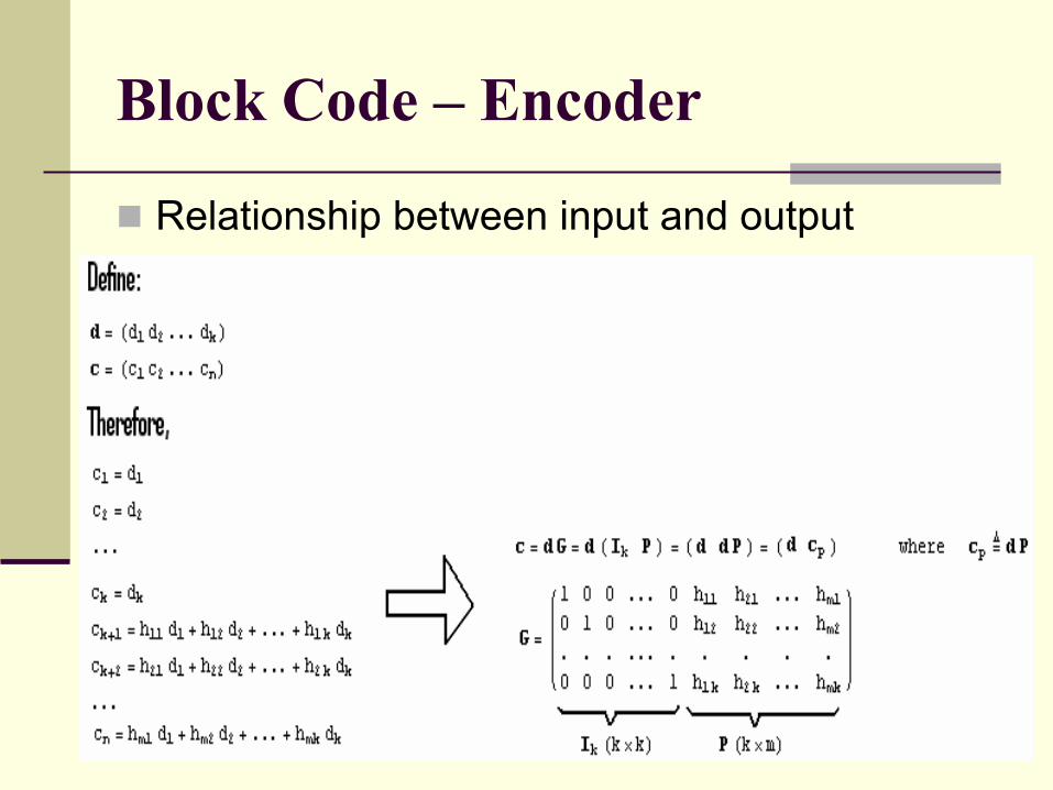
Number of bits in a data word = kNumber of bits in a code word = nParity-check bits = m = n – k

Block Code – Encoder

Relationship between input and output

Block Code – EncoderExample 1: The generator matrix G for a (n = 7, k = 4) Bose-Chaudhuri-Hocquenghen (BCH) code that is capable of correcting up to t = 1 bit error is shown below.

G=

ikjjjjjjjjj1 0 0 0 1 1 00 1 0 0 0 1 10 0 1 0 1 1 10 0 0 1 1 0 1

y{zzzzzzzzz = H I4 PL I4 =

ikjjjjjjjjj 1 0 0 00 1 0 00 0 1 00 0 0 1

y{zzzzzzzzz P=

ikjjjjjjjjj1 1 00 1 11 1 11 0 1

y{zzzzzzzzz

Block Code – Decoder

Step 1: Recognize the modulo-2 sum of any matrix (whose elements are binary) with itself is zero. Therefore,

Step 2: Due to noise, the n-bit received word is r = c ⊕ e

Step 3: Calculate the syndrome matrix s

0= cp+cp = dP+cp = H d cp L J PIm

N = cJ PIm

N = cHT where H=∆ H PT Im L

s = r HT = c + e HT = c HT + e HT = 0 + e HT

Block Code – Decoder

Step 4: Knowing r the syndrome matrix s can be computed. Next, e matrix can be inferred from the equation above. Once this is done, the original code word c can be constructed by performing the following operation:

c = r ⊕ e

Step 5: The decoder then converts this code word c to its corresponding data word d using a look-up table similar to the one shown in Slide 6.

Block Code - Decoder

Example 2: Let the received 7-bit (n = 7) word be r = (1 1 0 1 1 0 1) and assume (n = 7, k = 4) BCH code is used as in Example 1. The H matrix and the syndrome matrix s can be computed as shown below.

H= H PT Im=n−k=7−4=3L =ikjjjjj 1 0 1 1 1 0 01 1 1 0 0 1 00 1 1 1 0 0 1

y{zzzzzs= rHT = H 1 1 0 1 1 0 1L

ikjjjjjjjjjjjjjjjjjjjjj1 1 00 1 11 1 11 0 11 0 00 1 00 0 1

y{zzzzzzzzzzzzzzzzzzzzz = H 1 0 1L

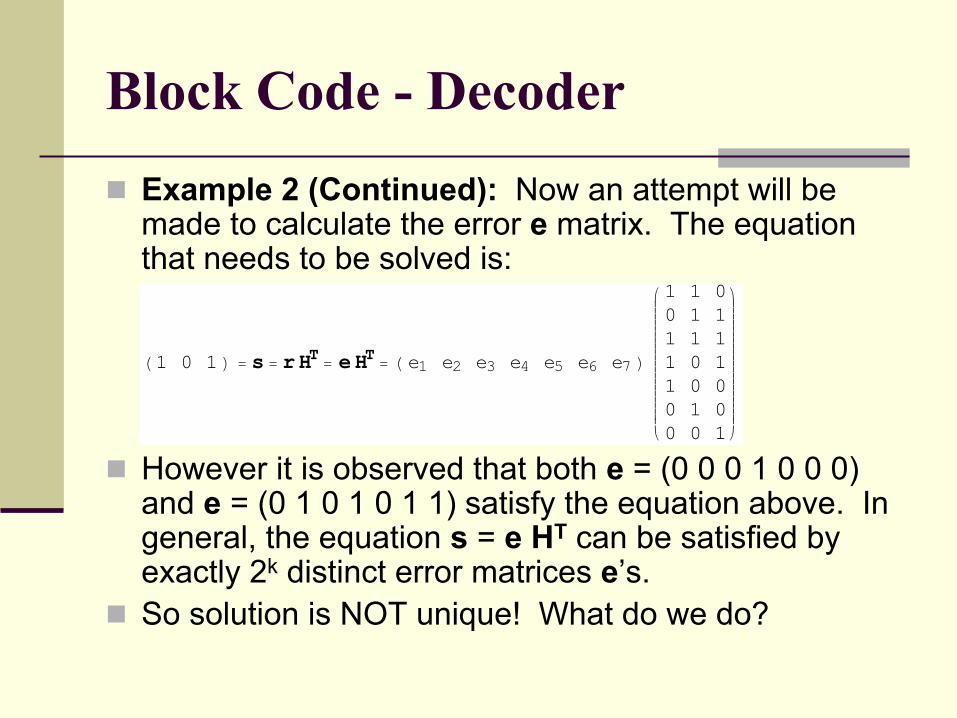
Block Code - DecoderExample 2 (Continued): Now an attempt will be made to calculate the error e matrix. The equation that needs to be solved is:

However it is observed that both e = (0 0 0 1 0 0 0) and e = (0 1 0 1 0 1 1) satisfy the equation above. In general, the equation s = e HT can be satisfied by exactly 2k distinct error matrices e’s. So solution is NOT unique! What do we do?

H1 0 1L = s = rHT = eHT = H e1 e2 e3 e4 e5 e6 e7 L

ikjjjjjjjjjjjjjjjjjjjjj1 1 00 1 11 1 11 0 11 0 00 1 00 0 1

y{zzzzzzzzzzzzzzzzzzzzz

Block Code - Decoder

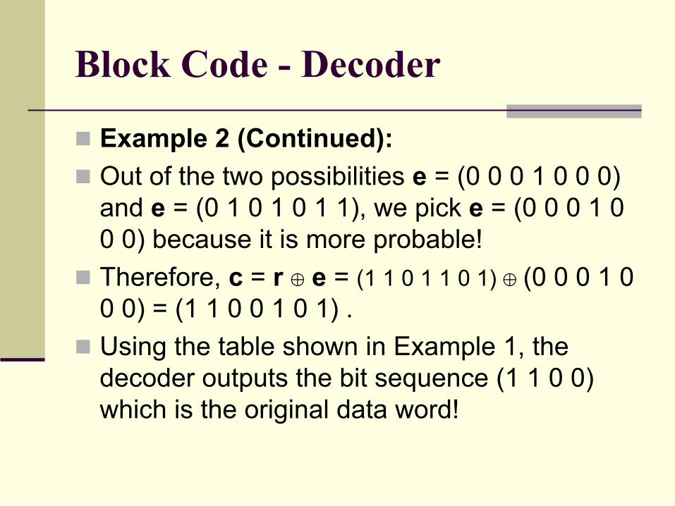
Example 2 (Continued):Out of the two possibilities e = (0 0 0 1 0 0 0) and e = (0 1 0 1 0 1 1), we pick e = (0 0 0 1 0 0 0) because it is more probable!Therefore, c = r ⊕ e = (1 1 0 1 1 0 1) ⊕ (0 0 0 1 0 0 0) = (1 1 0 0 1 0 1) . Using the table shown in Example 1, the decoder outputs the bit sequence (1 1 0 0) which is the original data word!

Block Code – Generator Matrix G

In Example 1 & 2, encoding and decoding steps are fairly straightforward once generator matrix G is given. How to determine G matrix in the first place?In this project, two popular methods known as the Bose-Chaudhuri-Hocquenghen (BCH) code and Reed-Solomon (RS) code can be used. Built-functions are also available in MATLAB communication tool box that can generate the G matrix.

Block Code – Coding Efficiency

Defined as k / nCoding Efficiency [n/k] vs. # of Correctible Errors [t]

Coding Scheme = Block Code [BCH Method]

0

0.1

0.2

0.3

0.4

0.5

0.6

0.7

0.8

0.9

1

0 20 40 60 80 100 120

# of Correctible Errors [t]

Cod

ing

Effic

ienc

y [n

/k]

n=7 n=15 n=31 n=63 n=127 n=255 n=511

Coding Efficiency [n/k] vs. # of Correctible Errors [t] Coding Scheme = Block Code [RS Method]

0

0.1

0.2

0.3

0.4

0.5

0.6

0.7

0.8

0.9

1

0 50 100 150 200 250# of Correctible Errors [t]

Cod

ing

Effic

ienc

y [n

/k]

n=7 n=15 n=31 n=63 n=127 n=255 n=511

BCH Block code scheme RS Block code scheme

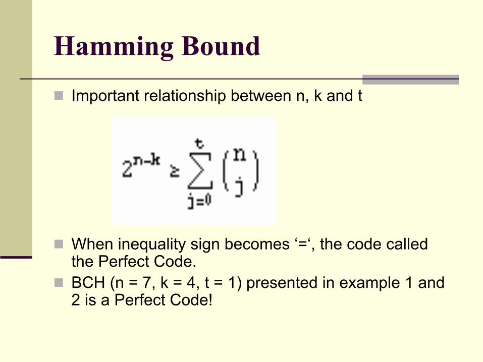
Hamming BoundImportant relationship between n, k and t

When inequality sign becomes ‘=‘, the code called the Perfect Code.BCH (n = 7, k = 4, t = 1) presented in example 1 and 2 is a Perfect Code!

Block Code - Interleaving

Interleave the bit sequence before transmission can guard against burst error!First three codes words to be transmitted are (Assume burst errors have occurred in the boxes that are shaded): x= H x1 x2 ... x15L

y= H y1 y2 ... y15Lz= H z1 z2 ... z15L

Simulation Setups

Simulation Results BER vs. SNR [dB] Coding Scheme = BCH

1.E-06

1.E-05

1.E-04

1.E-03

1.E-02

1.E-01

1.E+0023 25 27 29 31 33 35

SNR [dB]

BE

R

BER [BCH(7,4,1)] BER [BCH(15,7,2)]BER [BCH(31,16,3)] BER [Uncoded]

BER vs. SNR [dB} Coding Scheme = RS

1.E-06

1.E-05

1.E-04

1.E-03

1.E-02

1.E-01

1.E+0023 25 27 29 31 33 35

SNR [dB]B

ERBER [RS(7,5,1)] BER [Uncoded]BER [RS(7,3,2)] BER [RS(7,1,3)]

Simulation ResultsBER vs. Fiber length [km] Coding Scheme = RS

0.E+00

5.E-03

1.E-02

2.E-02

2.E-02

3.E-02

3.E-02

0 20 40 60 80 100Fiber Length [km]

BER

BER [RS(7,5,1)] BER [Uncoded]BER [RS(7,3,2)] BER [RS(7,1,3)]

BER vs. Fiber length [km] Coding Scheme = BCH

0.E+00

5.E-03

1.E-02

2.E-02

2.E-02

3.E-02

3.E-02

0 20 40 60 80 100Fiber length [km]

BER

BER [BCH(7,4,1)] BER [BCH(15,7,2)]BER [BCH(31,16,3)] BER [Uncoded]

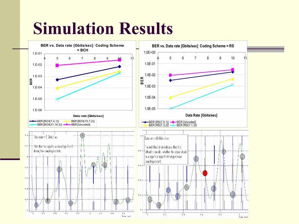
Simulation ResultsBER vs. Data rate [Gbits/sec] Coding Scheme

= BCH

1.E-06

1.E-05

1.E-04

1.E-03

1.E-02

1.E-014 5 6 7 8 9 10 11

Data rate [Gbits/sec]

BER

BER [BCH(7,4,1)] BER [BCH(15,7,2)]BER [BCH(31,16,3)] BER [Uncoded]

BER vs. Data rate [Gbits/sec] Coding Scheme = RS

1.0E-05

1.0E-04

1.0E-03

1.0E-02

1.0E-01

1.0E+004 5 6 7 8 9 10 11

Data Rate [Gbits/sec]

BER

BER [RS(7,5,1)] BER [Uncoded]BER [RS(7,3,2)] BER [RS(7,1,3)]

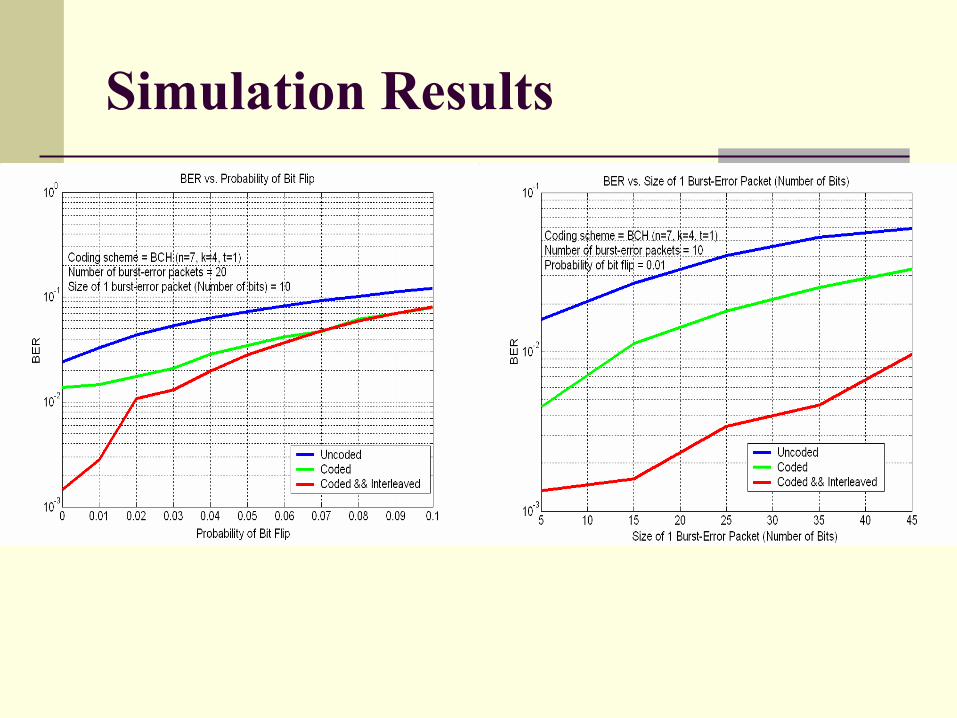
Simulation Results

Simulation Results

Now, my partner Christian will talk about convolutional code.

A brief history of convolutional codes

Coding method invented by Elias (1955)Effective decoding algorithm by Viterbi (1967)Various applications in deep-space / satellite / mobile communicationsNow giving way to a new generation of codes, Turbo Codes (1993)However, this is not the end – convolutional codes and their concepts still remain important as a part of Turbo Codes

Convolutional Codes vs. Block Codes

We do not have the notion of a block lengthAn input stream of bits is coded into an output stream of bitsThe output does not only depend on the input, but also on the last m inputs.

Encoder is not stateless, it has memory.

A simple example, the encoder

Input bit together with two previous bits form new output codeword by mod-2 addition.Code rate is 1/2, for each input bit we get two output bits.After each clock cycle, we shift the bits to the right.

xi-1 xi-2 c1i

c2i

xi

The encoder in action

0 0 1

1

1,0,0,1

The encoder in action

1 0 1

1

1,0,0

11,

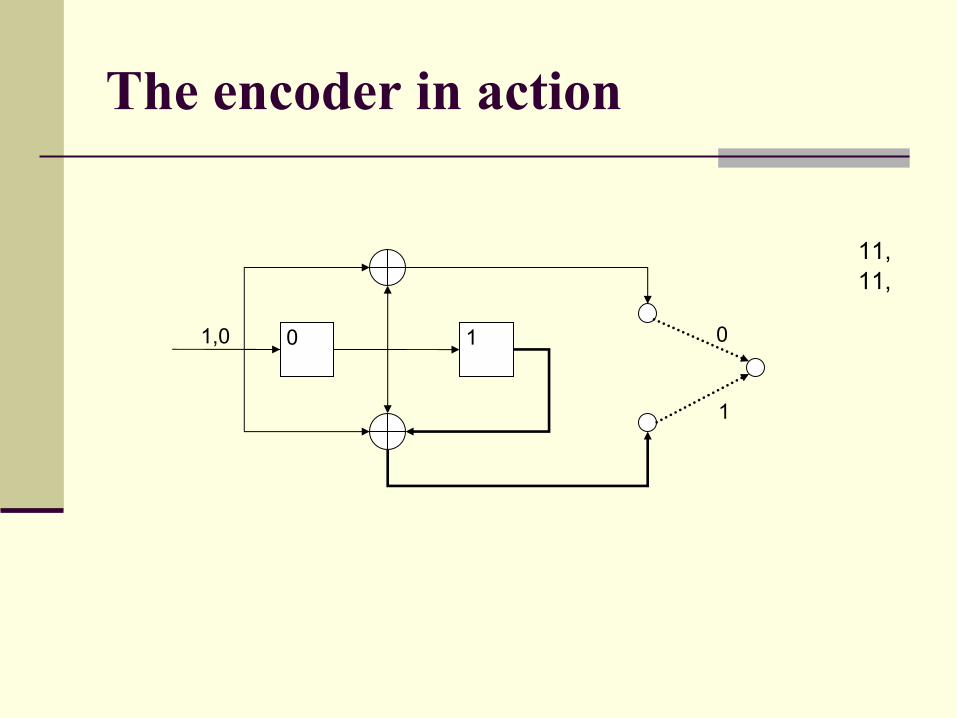
The encoder in action

0 1 0

1

1,0

11,11,

The encoder in action

0 0 1

1

1

11,11,01,

Encoder is a finite state machine

Memory cells capture the state {00,01,10,11}Transitions between states are visualized with arrowsxi / c1i c2i at the edges of the graph tell us input and output bitsThis is useful for drawing the trellis diagram

00

11

1001

1/11

1/00

0/11

0/10

0/01

0/10

0/00

1/01

Trellis Diagram

Also describes state machine, but focuses on time domainStates are on horizontal levels, transitions are also arrowsDotted / solid lines are for input bit 0 / 1.We always start in state (00)

00 00 00 00

00 00 00

11 11 11 11

01 01

10 10

11 11 11

10 10

01 01

(00)

(01)

(10)

(11)

Transmission of sequence (1,0,0,1)is printed in bold

How can we decode this stream?

We do not have separate code words, so we cannot use translation tablesWe need an algorithm that can deal with long bit sequences

Trellis diagram will help

MysteriousBlackBox

1,0,0,1, … 11,11,01,11, …=???

Decoding: Viterbi’s AlgorithmAssume the encoder‘s output was (11,11,01,11) but one bit was corrupted by a very nasty nonlinearity.

(00)

(01)

(10)

(11)

2

0

00

11

11 10 01 11

•We first receive (11)

•But we do not believe that this is correct –we never know

•The received (11) could as well be a (00) that was corrupted by two errors!

•Bookkeeping: We write the number of errors next to the arrows

Decoding: Viterbi’s Algorithm

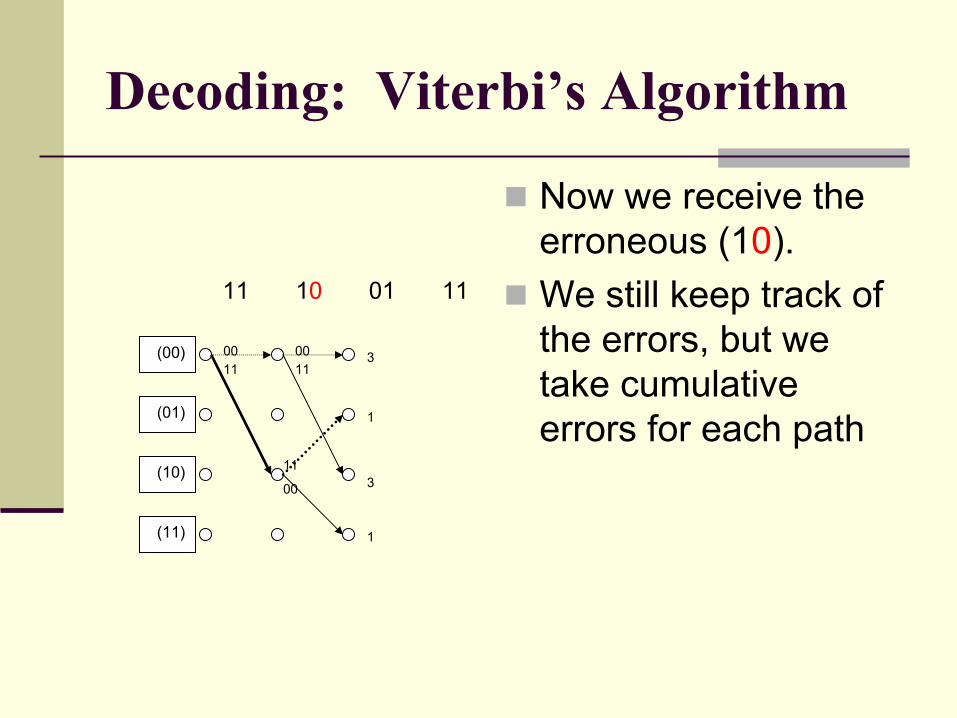
Now we receive the erroneous (10).We still keep track of the errors, but we take cumulative errors for each path

00 00

00

11 11

11

(00)

(01)

(10)

(11)

3

1

3

1

11 10 01 11

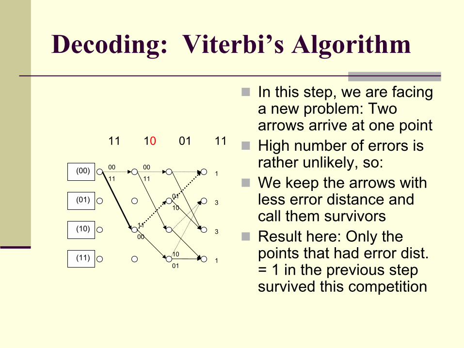
Decoding: Viterbi’s AlgorithmIn this step, we are facing a new problem: Two arrows arrive at one pointHigh number of errors is rather unlikely, so:We keep the arrows with less error distance and call them survivorsResult here: Only the points that had error dist. = 1 in the previous step survived this competition

00 001

00

11 11

011

11

10

3

10

013

(00)

(01)

(10)

(11)

11 10 01 11

Decoding: Viterbi’s AlgorithmAt the end, we only have four paths left that we consider likely enoughOne of them is the path printed in bold The original sequence!

00

00

11 11

01 01

10

11

01

(00)

(01)

(10)

(11)

3

1

2

2

Our original sequence also has minimum error, so we choose it as the final survivorWe walk back the path and conclude from dotted / solid lines that the decoded message is (1,0,0,1)The error during transmission was corrected!

11 10 01 11

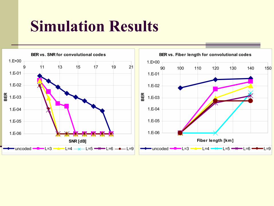
Simulation ResultsBER vs. SNR for convolutional codes

1.E-06

1.E-05

1.E-04

1.E-03

1.E-02

1.E-01

1.E+009 11 13 15 17 19 21

SNR [dB]

BER

uncoded L=3 L=4 L=5 L=6 L=9

BER vs. Fiber length for convolutional codes

1.E-06

1.E-05

1.E-04

1.E-03

1.E-02

1.E-01

1.E+0090 100 110 120 130 140 150

Fiber length [km]B

ERuncoded L=3 L=4 L=5 L=6 L=9

Simulation Results

BER vs. bit rate for convolutional codes

1.E-06

1.E-05

1.E-04

1.E-03

1.E-02

1.E-01

1.E+004 5 6 7 8 9 10 11

Bit rate [Gbit/s]

BER

uncoded L=3 L=4 L=5 L=6 L=9

Social & Economic BenefitsNot necessary to change existing network infrastructure since error correction can be performed at the receiver side.This can help save millions of dollars. User on the receiver end does not have to request for re-transmission from the sender. Thus communication is made more robust. As a consequence, several software programs out there such as Skype that rely on robust communication are becoming more popular among the general public as a cheap way to keep in touch with family and friends. This is a major social benefit that results from the use of FEC in communication.

Conclusion

Two classes of error control schemes are studied in this project and they are known as the block code and the convolutional code.

Simulation performed using MATLAB and RSoft Optsim demonstrates that these error-schemes are very powerful tools to reduce BER.

Bibliography[1] B. P. Lathi, Modern Digital and Analog Communication Systems, Oxford University Press 1998[2] W. W. Peterson and E. J. Weldon, Jr., Error Correcting Codes, 2nd ed., Wiley, New York, 1972[3] S. Lin and D. Costello, Error Control Coding: Fundamentals and Applications, Prentice-Hall, Englewood-Cliffs, NJ, 1983[4] MATLAB communication toolbox -http://www.mathworks.com/products/communications/functionlist.html[5] P. Elias, “Coding for noisy channels,” in IRE Conv. Rec., Mar. 1955, vol. 3, pt. 4, pp. 37–46[6] O. A. Sab and V. Lemarie, “Block turbo code performances for long-haul DWDM optical transmission systems,” in Optical Fiber Communication Conf., vol. 3, 2000, pp. 280–282.[7] A. J. Viterbi, “Error bounds for convolutional codes and an asymptotically optimum decoding algorithm,” IEEE Trans. Inform. Theory, vol. IT-13, pp. 260-269, Apr. 1967.[8] Charan Langton, Signal Processing & Simulation Newsletter, Tutorial 12, Website: http://www.complextoreal.com/convo.htm, accessed in May 2006[9] Thierry Turletti, From Speech to Radio Waves, Website: http://tnswww.lcs.mit.edu/~turletti/gsmoverview/node9.html, accessed in May 2006

~ The End ~