The Role of Capital Structure in Cross-Sectional...

The Role of Capital Structure in Cross-Sectional Tests of Equity

Returns ∗

Anchada Charoenrook†

This version: January, 2004

∗I would like to thank Joshua D. Coval, Wayne E. Ferson, William N. Goetzmann, Eric Ghysels, David Hirshleifer,Phil Howrey, Gautam Kaul, Craig Lewis, Ronald Masulis, Tyler Shumway, Douglas Skinner, Richard Shockley, HansStoll, and Anjan V. Thakor for helpful comments. All errors are the responsibility of the author.

†The Owen Graduate School of Management, Vanderbilt University, 401 21st. Avenue South, Nashville TN 37215.Phone: (615) 322-1890 Fax: (615) 343-7177 Email: [email protected]

1

The Role of Capital Structure in Cross-Sectional Tests of Equity Returns

Abstract: This paper examines the impact of time varying capital structure in cross-sectional

tests of equity returns (the capital structure effect). Theoretical analysis yields very different em-

pirical implications and interpretations than is common in the asset pricing literature. The analysis

shows that the capital structure effect biases regression coefficients in the Fama and MacBeth (1973)

estimation, and can induce the relation between size or book-to-market and equity returns. A new

empirical test that distinguishes this explanation from other explanations in the literature reveals

that in a cross section of equity returns the capital structure effect accounts for at least 50% of the

explanatory power of size and 70% of the explanatory power of book-to-market.

1 Introduction

Over the last two decades, empirical studies applying the Fama and MacBeth (1973) cross-sectional

test of average returns report consistent evidence that size and book-to-market (BE/ME) are related

to average equity returns, while the Capital Asset Pricing Model (CAPM) beta is not (See, for

example, Banz (1981), Fama and French (1992), Fant and Peterson (1995), Kothari, Shanken, and

Sloan (1995), Jaganathan and Wang (1996), Knez and Ready (1997), and Davis, Fama, and French

(1999)). The interpretation of these findings is central to understanding what risks determine

expected stock return. In this study, I reexamine this evidence recognizing that financial leverage,

which differs dramatically across firms and is time varying, can have an important impact on stock

return patterns. This analysis leads to a reassessment of implications of a large body of empirical

work testing the determinants of expected stock returns.

A number of interpretations of the size and book-to-market evidence have been offered in the

literature. One line of thinking is that expected equity return is determined by a multifactor model.

Size and BE/ME proxy for factor loadings on macroeconomic risks that are not captured by the

Sharpe Lintner CAPM beta. For example, Chan and Chen (1991), Fama and French (1992, 1995,

1996), and Berk, Green, and Naik (1999) suggest that size and BE/ME proxy for a factor loading

on financial distress risk that varies inversely with business cycle. Lettau and Ludvigson (2001)

report that the log of consumption-wealth ratio, which captures economic cycles, performs as well

as size and BE/ME in explaining the cross-section of equity returns. Berk (1995) points out that

there is an intrinsic relationship between the market values of stocks and expected returns. Given

relatively stable dividend policy, a rise in future expected returns requires current stock price to

decline. Thus, any variable that includes a measure of price such as size or BE/ME is related to

expected return when a risk factor is unaccounted for in asset pricing model estimates.

Other researchers argue that parameter estimates of size and BE/ME are biased due to an errors

in variables problem in the CAPM beta estimates that attenuate their statistical significance.1 In

recent work Ferguson and Shockley (2003) show that there is an errors in variables problem due to

estimating a CAPM beta using market equity returns rather than including both equity and debt1For example, Kim (1995) shows that correcting for an errors in variables problem in the CAPM beta diminishes

the size effect.

1

returns in the market index, which is theoretically more accurate. This creates a bias in the size

and BE/ME parameter estimates.

On the other hand, a number of researchers have challenged the validity of efficient market

hypothesis arguing that conditional on the validity of conventional specifications of the asset pricing

model, size and BE/ME are firm characteristics unrelated to factor loadings. These researchers

conclude that size and BE/ME are related to future returns of stocks because market participants

misprice stocks. That is, small size and high BE/ME firms are undervalued with respect to their

fundamental risks.2 Despite considerable debate over the interpretation of size and BE/ME evidence

and the appropriate specification for testing the CAPM, to date the literature has come to no

consensus.

This study proposes an alternative explanation for the size and BE/ME effect, and presents new

supporting empirical evidence. The explanation is based on a fundamental observation made by

Black and Scholes (1973) in their seminal paper on option pricing. In any linear factor model, each

factor loading on a levered firm consists of a factor loading on the firm assets (the unlevered firm)

multiplied by the elasticity of equity price with respect to the underlying asset price (henceforth

referred to as the price elasticity).3 A factor loading on firm asset returns measures exposure of

firm assets to an economic risk, while the price elasticity measures the added risk exposure due to

financial leverage. In the context of the CAPM, equity beta is a product of the firm’s asset beta

multiplied by an elasticity term, which is a non-linear function of the firm’s debt-to-equity ratio,

measured in market value terms. Empirical tests here reveal that size and BE/ME are correlated

with the debt-to-equity ratio, and thus they are also correlated with price elasticity. The hypothesis

that size and BE/ME are related to expected equity returns because they proxy for price elasticity,

rather than for firm exposure to a particular risk factor is formally tested in this study. This

alternative explanation is termed the capital structure effect.

This paper provides two fundamental contributions. First, it provides a theory that explicitly

shows how the capital structure effect can induce a relationship between size or BE/ME and2See for example, Lakonishok, Shleifer, and Vishny (1994), Daniel and Titman (1997), Daniel, Hirshleifer, and

Subrahmanyam (1998).3For a detail discussion on this topic see Hamada (1971) for the case of riskless debt and Galai and Masulis (1976)

for debt with default risk.

2

expected equity returns. The theory developed here has several new empirical implications.4 First,

if the asset pricing model estimated is missing any risk factor, size and BE/ME will be related to

expected equity returns because they proxy for the price elasticity component of the missing factor.

Second, even if an economist identifies every risk factor that is priced, in cross sectional analysis

size and BE/ME will still be related to expected equity returns. This is because estimation of a

conditional factor loading in a Fama-MacBeth framework assumes that a factor loading is constant

for a period of five years. Capital structure, however, varies continually over this five-year period.

When firms keep their debt levels relatively constant and stock prices change, a systematic error,

which is correlated with the debt-to-equity ratio, is introduced in the factor loading estimates.

The error biases the coefficient estimates of factor loadings tested and of size and BE/ME.5 This

theoretical result highlights a problem in current test procedures. The coefficient estimate of any

factor loading which is obtained by estimating the Fama-MacBeth first pass regression using levered

equity returns is biased. Whether the bias is empirically significant or not is an empirical question

which is explored here. Third, the relations between stocks and size or BE/ME are stronger for

firms exhibiting higher leverage, everything else equal.6 Finally, size and BE/ME should not be

empirically important in explaining expected firm returns.

Differentiating the capital structure effect from a distress risk factor effect is an important

issue. It can resolve whether there is a distinct bankruptcy or financial distress risk factor related

to economic cycles that causes a shift in the investment opportunity set of the marginal investor.

If size and BE/ME proxy for a price elasticity and not for additional fundamental risk factors, the

conventional use of factors SMB and HML as linear risk factors to evaluate the systematic risk

of equity is brought into question.7 Furthermore, if size and BE/ME proxy for the stock return

elasticity, their relationships to equity returns is not counter factual evidence on the empirical

validity of the conventional specification of the CAPM or of market efficiency.

Established empirical methods test the effect of leverage by incorporating an additional leverage

proxy term in a linear asset pricing model.8 This method suffers from a well known fundamental4See Black and Scholes (1973), Merton (1974), and Galai and Masulis (1976).5Baker and Wurgler (2002) find that firms try to time the market when issuing debt, and firms keep debt levels

constant for a long period of time.6This is consistent with empirical evidence reported in Knez and Ready (1997).7SMB and HML are factors created from portfolios of size and BE/ME proposed by Fama and French (1995).8See, for example, Bhandari (1988) and Fama and French (1992)

3

drawback; it concurrently tests multiple hypotheses. Furthermore, the elasticity term is a non-

linear function of the debt-to-equity ratio, and it multiplies firm-level factor loadings. Due to

non-linearity, accounting for the capital structure effect by adding a leverage measure in a linear

asset pricing model is ineffective.9

The second contribution of this study is to develop an empirical test which distinguishes between

the capital structure effect and other explanations. This test exploits the theoretical implication

that size and BE/ME should not be empirically important in explaining expected firm returns.

Comparing Fama-MacBeth estimates of equity and firm return factor loadings yields a method for

testing the capital structure effect. For example, if size is a proxy for a distress factor, then size

should explain the cross-section of both firm returns and equity returns, and the price of risk should

be the same in both cases. Similarly, there should be an intrinsic relationship between size and firm

returns if a risk factor is missing. Alternatively, if markets are inefficient with respect to equity

returns, they should be inefficient with respect to firm returns as well. But if capital structure is

the cause for equity returns being related to size or BE/ME there should be no relations between

firm returns and either size or BE/ME.

Empirical tests presented here are based on monthly equity returns and firm returns of NYSE,

Nasdaq, and AMEX listed companies over the period from June 1963 through July 1998. Firm

returns are estimated from weighted average of equity and debt returns. Comparisons between

tests of firm returns and equity returns for the same set of firms demonstrate that in a cross section

of equity returns at least 50% of the explanatory power of size and 70% of the explanatory power

of BE/ME are due to the capital structure effect.10

9This may explain why some empirical studies such as Bhandari (1988) and Fama and French (1992), find thatadding a leverage proxy as another linear term in the Fama-MacBeth test does not change the cross-sectional coeffi-cients of size or BE/ME.

10In a contemporary work, Hecht (2002) empirically tests equity, firm, and bond returns to support or reject amodel of rational equilibrium, and Hectch reports similar empirical findings on BE/ME. My work differs from hisstudy in two respects. First, I analyze the effect of a time-varying capital structure on the Fama-MacBeth test ofequity returns, and I use firm returns in testing the theory. Second, my data set is different. Hecht studies the periodfrom 1973 through 1997 with an average of approximately 450 observations per month; the data set used here hasan average of 2700 observations per month. The longer period allows for an examination of the relationship betweensize and expected firm returns over varying market conditions; this relationship is not statistically significant afterthe 1970s, which is the shorter period that Hecth studies. A larger sample size also improves the power of the testshere.

4

2 The capital structure effect

The theoretical analysis of the capital structure effect proceeds in two steps. The equity return

process of a firm is derived from a return on its assets that is assumed to be lognormal. Then two

scenarios of the Fama and MacBeth (1973) (FM) test are analyzed using this levered equity return

process.

Assume there are two orthogonal marketwide variations denoted by Wl,t, for l ∈ [1, 2].11 Let

the asset return follow a lognormal process. Under widely accepted market conditions and without

assumptions about a specific capital structure policy of a firm, the excess equity return process of

firm i at time t, ri,t, is given as

ri,t = νi,tβ̄i1,tλ1,t + νi,tβ̄i2,tλ2,t +∫ 2∑

l=1

νi,tσ̄il,t dWl,t +∫νi,tσ̄i,t dεi,t. (1)

All derivations are provided in the appendix. The parameter σ̄il,t is the conditional covari-

ance of the asset return with marketwide variations, and σ̄i,t is the conditional firm-specific varia-

tion. They are non-stochastic. Both dWl,t and dεi,t are standard Brownian motion processes and

E[dWl,t dεi,t] = 0. A line over a parameter denotes a parameter associated with firm value.

The variable β̄il,t is the firm-level factor loading defined as β̄il,t ≡ Cov(r̄i,t,Wl,t)/V ar(Wl,t),

where r̄i,t is the return on the assets of the firm. The variable νi,t is the elasticity of the stock

price with respect to the value of the assets of the firm defined as νi,t ≡ ∂Si,t

∂Vi,t

Vi,t

Si,t, where Si,t and

Vi,t denote equity price and firm value of firm i at time t. The price elasticity νi,t is a constant one

for unlevered firms. It is a function of the debt-to-equity ratio for levered firms, and under general

assumptions it is an increasing function of the debt-to-equity ratio.12

The equity return process in (1) illustrates that the conditional equity beta, the correlation of

equity return with marketwide variations, and firm-specific volatility equal the respective firm pa-

rameters multiplied by νi,t. Therefore these equity level parameters increase with a firm’s leverage.

11The appendix derives the equity return process for any arbitrary number of marketwide variations.12It is shown in the appendix that, under the assumptions of the Merton (1974) capital structure model, price

elasticity increases with the debt-to-equity ratio.

5

This is consistent with existing empirical evidence.13

Harvey and Siddique (2000) find that the conditional skewness of equity returns declines with

size but increases with BE/ME. According to Equation (1), when there is a negative shock to

returns, leverage increases, and νi,t increases, causing further increases in volatility. This interaction

generates more negative skewness in the probability distribution of equity returns of firms with

higher debt-to-equity ratios. The empirical test results presented below reveal that size is negatively

correlated and BE/ME is positively correlated with the debt-to-equity ratio. Thus, leverage may

explain why size and BE/ME forecast conditional skewness in the cross-section of equity returns.

2.1 The Fama-MacBeth cross-sectional test of levered equity returns

The Fama-MacBeth test and its variants consist of two regressions.14 The first-pass regression

estimates the CAPM equity beta by estimating the market model using three to five years of

historical monthly return data, assuming that beta is constant. The CAPM beta estimate is then

employed as an independent variable in the second-pass regression. The second-pass regression is a

time series of cross-sectional ordinary least squares or weighted least squares regressions of excess

returns, ri,t, on one or more independent variables, Xil,t, that are candidates for factor loadings.

For each test period, from t = 1, . . . , T , and for N independent variables the regression is:

ri,t = λ̂0,t +N∑

l=1

λ̂l,tXil,t + ξi,t, (2)

where ξi,t is the residual error term. The hat symbol denotes an estimated variable. The time series

average of the cross-sectional regression coefficients of the factors is estimated from λ̂l = 1T

∑Tt=1 λ̂l,t.

Each average slope is tested against the hypothesis that it is zero to identify which risk factors

determine expected returns.

When levered equity returns are involved in the Fama-MacBeth test, I show that size and

BE/ME may explain average returns even though they are unrelated to any risk factors. That is,13Christie (1982), for example, reports that the variance of equity returns increases with the level of leverage.

DeJong and Collins (1985) find that firms with higher leverage have more unstable equity beta than firms with lessleverage.

14For a comprehensive review of the two-pass test of beta models, see Shanken (1992).

6

size and BE/ME are independent of dW1,t, dW2,t, β̄i1,t, or β̄i2,t.

2.2 If the asset-pricing model is missing a risk factor

Suppose we test an asset pricing model that is missing one factor from what would be the true

model, but that includes either size or BE/ME (denoted here by Xi,t as one of the independent

variable). The Fama-MacBeth cross-sectional regression is given as

ri,t = λ̂0,t + λ̂1,tβi1,t + λ̂X,tXi,t + ξi,t. (3)

When this regression is estimated using levered equity returns from Equation (1) the time series

average of the cross-sectional regression coefficient of size or BE/ME is

λ̂X = Et[λ̂X,t] =Et[Ei[β̄i2,t]]Et[λ2,t]Et[Covi(νi,t, Xi,t)]

Vari(Xi,t). (4)

The Covi(·, ·) denotes the covariance in the cross-section of firms. Since the time series and cross-

sectional average of firm-level factor loading Et[Ei[β̄i2,t]] > 0, and the risk premium of the missing

factor Et[λ2,t] > 0, the average slope of size or BE/ME, λ̂X , is not zero but has the same sign as

the correlation between size or BE/ME and νi,t.

The derivation of Equation (4) assumes that neither size nor BE/ME is related to any economic

risk factor. Yet size and BE/ME explain the cross-section of average equity returns. The intuition

for this result is that size or BE/ME proxies for νi,t which is a component of the equity-level factor

loading of the missing factor.

[Insert Figure 1 here]

Is size or BE/ME correlated with νi,t? Although νi,t is unobserved, it increases with the debt-to-

equity ratio of a firm. Therefore, if size or BE/ME is correlated with the debt-to-equity ratio, it is

correlated with νi,t as well. Figure 1a reports the time series of monthly cross-sectional correlations

between size and the debt-to-equity ratio and BE/ME and the debt-to-equity ratio from July 1967

through June 1998. The correlation between size and the debt-to-equity ratio is negative in 96.7%

7

of the months and the time series average of these correlations is -0.07, which is significant at a 1%

level (Table 1). This correlation is negative and higher in magnitude during all months before 1972.

The correlation between BE/ME and the debt-to-equity ratio is positive in all months (second plot

in Figure 1a). The time series average of this correlation is 0.258, which is significant at a 1% level.

[Insert Table 1 here]

The conditional price elasticity νi,t can be calculated from firm characteristics assuming a specific

capital structure model. Using the Merton (1974) capital structure model and data described below

I estimate the conditional price elasticity for each firm each month. The monthly cross-sectional

correlation of size and νi,t is negative in most months, and the correlation of BE/ME and νi,t is

positive in all months (Figure 1b). The time series average of the correlation of size and νi,t is

-0.064 and that of BE/ME and νi,t is 0.259 (Table 1).

These empirical findings suggest a capital structure effect as follows. The average slope coef-

ficient of size in the Fama-MacBeth test is negative, and it is steeper prior to 1972. This may

explain the empirical puzzle of why size does not explain the cross-section of equity returns after

the early 1970s. The capital structure effect predicts that the average slope of BE/ME is positive.

Furthermore, since BE/ME and the debt-to-equity ratio or νi,t are more correlated than size and

the debt-to-equity ratio or νi,t, Equation (4) predicts that the average slope of BE/ME will be

steeper than the average slope of size. This is consistent with the empirical evidence reported in

Fama and French (1992 and 1996). Finally, since νi,t is constant for firms, size and BE/ME should

not explain the cross-section of average firm returns.

2.3 If a factor loading is estimated from Fama-MacBeth first pass regression

When a factor loading such as the CAPM beta is unobservable, it is obtained from the first-pass

regression of the Fama-MacBeth test by estimating the market model using returns for 60 months

immediately prior to the test period. Given the time variation of leverage during this estimation

period, the estimated factor loading is subjected to errors in variables correlated with the debt-

to-equity ratio. To see why, let the second risk factor in Equation (1) be the market factor. Let

8

βi2,l denote the true conditional CAPM equity beta, and let β̂i2,t denote the conditional CAPM

equity beta estimate. Define the estimation error as errori,t ≡ β̂i2,t − βi2,t. Now assume a firm’s

value increases steadily during the beta estimation period while debt remains relatively constant.

Its debt-to-equity ratio drops and its equity beta declines. The equity beta is estimated over a

60-month period, therefore it equals the average of equity betas during these 60 months, which

is higher than the true conditional equity beta at the end of the 60-month period. Thus, at the

test period, when the debt-to-equity ratio is low, the estimation error is positive (see Figure 2).15

Similarly, when firm value declines steadily during the beta estimation period, at the test period,

the true conditional beta is higher than the beta estimate, and the estimation error is negative.

Therefore, the estimation error is negatively correlated with the debt-to-equity ratio of that firm.

[Insert Figure 2 here]

Now suppose we test a cross-sectional regression model that has the two correct factor load-

ings, and let the second factor loading be the conditional CAPM beta estimated from the Fama-

MacBeth’s first-pass regression. In this case, the model tested is well specified, but the CAPM

equity beta is estimated with systematic error. Let the model also include either size or book-to-

market denoted by Xi,t as one of the independent variables as follows:

ri,t = λ̂0,t + λ̂1,tβi1,t + λ̂2,tβ̂i2,t + λ̂X,tXi,t + ξi,t. (5)

In this case, the time series average of the cross-sectional regression coefficient in the Fama-MacBeth

test of the CAPM beta is given as:

λ̂2 = Et[λ2,t] +Et[Ei[β̄i2,t]]Et[λ2,t]Et[Covi(νi,t, errori,t)]

Vari(β̂i2,t). (6)

Since νi,t is an increasing function of the debt-to-equity ratio, and it has been established that

errori,t is negatively correlated with the debt-to-equity ratio, Covi(νi,t, errori,t) < 0. We also have

that Et[λ2,t] > 0, and Et[Ei[β̄i2,t]] > 0, therefore the second term on the right-hand side of Equation

(6) is negative, Thus the average slope of the CAPM beta is negatively biased.15It is assumed that firm beta and the debt-to-equity ratio are not correlation or that they are not so highly

negatively correlated as to negate the results given here.

9

The average slope of size or BE/ME is given as:

λ̂X =Et[(λ2,t − λ̂2,t)]Et[Ei[βi2,t]]Et[Covi(νi,t, Xi,t)]− Et[λ̂2,t]Et[Covi(errori,t, Xi,t)]

Vari(Xi,t). (7)

To examine λ̂X , we establish a sign for each term in Equation (7). As the average slope of the

CAPM beta is negatively biased, Et[(λ2,t − λ̂2,t)] > 0. Second, the term Et[Covi(νi,t, Xi,t)] has

the same sign as the correlation between the debt-to-equity ratio and Xi,t. Finally, the term

−Et[λ̂2,t]Et[Covi(errori,t, Xi,t)] has the same sign as the correlation between the debt-to-equity

ratio and Xi,t, because the error term is negatively correlated with the debt-to-equity ratio. There-

fore, the average slope of Xi,t is biased in the direction of the correlation between the debt-to-equity

ratio and Xi,t. Because size and BE/ME are negatively and positively correlated with the debt-to-

equity ratio, the capital structure effect predicts that the average slope of size is negative and of

BE/ME is positive.

The intuition for this result is that the CAPM beta estimated from the Fama-MacBeth first-

pass regression entails an error that is negatively related to the debt-to-equity ratio. The effect of

this error in variables is to negatively bias the average regression coefficient of the CAPM beta,

and to bias the average regression coefficient of other independent variables in the direction of

the correlation of that variable and the debt-to-equity ratio. This is the case not only for the

CAPM equity beta but also for any factor loading that requires an Fama-MacBeth model first pass

regression estimate.

3 Empirical Method

There are a two possible ways to test the effect of capital structure. First, test the conditional

model

Et[ri,t] = αi,t +2∑

l=1

νi,tβ̄il,tλl,t + λsizesize+ λBE/MEBE/ME, (8)

using the Fama-MacBeth test. The null hypothesis is λsize = 0, λBE/ME = 0, and λl,t = 0.

The problem with this approach is that it is a joint test of three hypotheses: 1) the tested

multifactor model is the correct asset pricing model; 2) size and BE/ME are related to expected

10

return due to the capital structure effect; and 3) the market is efficient. If, for example, λsize = 0 or

λBE/ME = 0 is rejected, it may be due to any of these three reasons: 1. the asset pricing model is

missing a risk factor and size or BE/ME is a proxy for νi,t of the missing factor, 2. size or BE/ME

is a proxy for a distress risk factor, or 3. small size and large BE/ME firms are mispriced. On the

other hand, if we find that λsize = 0 is not rejected, it could be because the CAPM model is not

the right model or that the capital structure effect is empirically insignificant. Most cross-sectional

tests of asset pricing models that have been proposed report low average R-squares indicating that

the models we currently have do not account for all risk factors.16 Hence, a conditional test will

not effectively distinguish the capital structure effect from other explanations.

An alternative test method is to compare cross-sectional tests of equity returns and firm returns

of the same set of firms. The difference between the time series averages of the regression coefficient

of size or BE/ME of firm returns and equity returns measures the capital structure effect separately

from other hypotheses outlined above. For example, if size or BE/ME proxy for a distress risk factor,

then size or BE/ME should also be related to the cross-section of firm returns. Any priced risk

factor should be present in both equity returns and firm returns, and the risk premium should be

the same. Moreover, if the stock market is inefficient, the inefficiency should be evident in both

equity and firm returns. If size or BE/ME proxy for νi,t, however, size or BE/ME should be related

to equity returns and not firm returns. The objective of this study is to isolate the capital structure

effect, so I adopt this method.

Test procedure using firm returns has a limitation that the estimated firm returns many still be

related to leverage because the estimation procedure does not eliminate the leverage effect from firm

returns. For example, the case when the functional relationship between equity and firm returns

is firm specific and unaccounted for by a firm return estimation procedure. This may be the case

when bankruptcy cost differs greatly among firms, the optimal capital structure differs among firm,

and thus the relationship between equity return and firm returns is firm specific. For this cases,

a procedure that compares the Fama-MacBeth time series averages of the regression coefficient of

equity and firm returns is a conservative test in the sense that it tests for the effect of leverage

that is accounted for in constructing firm returns and not for other leverage effects that remain in16See for example, Fama and French (1992), Jaganathan and Wang (1996), and Lettau and Ludvingson (2001).

11

firm return estimates. If the difference between time series averages of the regression coefficient of

equity and firm returns is significant and estimated firm returns are positively related to leverage,

then the overall leverage effects beyond that which is accounted for is even more important.

4 Data

The data set consists of all non-financial firms in the intersection of (1) the monthly return files

from the Center for Research in Security Prices (CRSP) from July 1963 through June 1998, (2)

the merged Compustat annual industrial files from 1962 through 1998, and (3) the CRSP monthly

US Government Bills, Notes, and Bonds supplemental files.17 Consistent with established practice

I exclude financial firms because the high leverage associated with them does not indicate financial

distress as would leverage in non-financial firms.

4.1 Firm returns

Firm returns are obtained from the weighted average of equity returns and bond returns as:

r̄i,t =Si,t

Vi,tri,t +

Di,t

Vi,trBi,t, (9)

where Si,t is the value of equity, Di,t is the total value of bonds, and the firm value is Vi,t = Si,t+Di,t.

Equity returns, ri,t, are from CRSP monthly files. The equity returns and equity value from July

of year t through June of year t + 1 are matched with monthly bond returns, rBi,t, and debt value

as measured by annual accounting ratios in December of year t− 1.18

Bond returns are returns of Treasury securities of the same maturity as the corporate bond

plus a bond risk premium. Maturities of corporate bonds are obtained from Compustat annual

industrial files. Compustat reports short-term debt and long-term debt maturing in years 1 through

5 after the year it is reported. Here, debt maturing in one year is computed as the sum of long-term

debt in current liabilities (data item 44), taxes payable (data item 71), and notes payable (data17I choose the 1962 Compustat start date because of serious selection bias in those data before then (Fama and

French (1992)).18The implicit assumption here is that, in pricing risk, investors care about annual changes in leverage ratios.

12

item 206). The amount of debt maturing in years 2, 3, 4, and 5 is obtained from data items 91,

92, 93, and 94, respectively. The remaining long-term debt, which equals long-term debt minus

long-term debt in current liabilities and debt maturing in less than five years, is assigned an average

maturity of ten years.19

The value of debt of firm i maturing in T years is di,t+T . The total debt outstanding, Di,t, is the

sum of debts maturing in years one through five and debt maturing beyond five years. The total

return on debt of a firm is calculated as a value-weighted average of monthly returns on Treasury

bonds of matched maturities plus the risk premium pi,t:

rBi,t =

5∑T=1

rgt+T

di,t+T

Di,t+ rg

t+10

di,t+10

Di,t+ pi,t, (10)

where rgt+T is the return on Treasury bonds maturing in T years.

The risk premium is obtained using the bond pricing model of Merton (1974). This model is

simple, and Sarig and Warga (1989) find that the time profile of the risk premium of corporate

bonds is consistent with the theoretical time profile produced by the Merton (1974) model.

In calculating the risk premium, I view firm’s debt as one composite bond whose time to

maturity, τ , is the weighted average of the time to maturity of the bonds outstanding, τ =∑5T=1 T

di,t+T

Di,t+ 10di,t+10

Di,t. The risk-free rate to maturity or the yield, yi,t, is the weighted aver-

age yield on Treasury bonds, yi,t =∑5

T=1 yt+Tdi,t+T

Di,t+ yt+10

di,t+10

Di,t, where yt+T is the yield of the

Treasury bond maturing in T years. The data on Treasury bond yields, bond returns, and the

risk-free rate are from the CRSP monthly US Government Bills, Notes, and Bonds supplemental

files.20

The risk premium is given as (Merton (1974)):

pi,t = −1τ

ln (1−N (−h−i,t) +Vi,t

Di,te−yi,tτN (−h+

i,t)), (11)

19I extrapolate the graph of the percentage of total debt maturing before year T as a function of T to the timewhen zero debt remains to obtain this 10 year estimate.

20One-year, two-year, three-year, four-year, and five-year bond yields are from the Famablis file. The ten-year bondyield is from CRSP fixed-term indices files. The bond returns are from Fama Maturity Portfolio Return files with12-month intervals.

13

where N (·) denotes the cumulative normal distribution. The variables h+i,t and h−i,t are given by

h+i,t ≡

ln(Vi,t/Di,t) + (yi,t + δ̄2i,t/2)τδ̄i,t√τ

,

and h−i,t ≡ h+i,t − δ̄i,t

√τ . The variable δ̄i,t denotes conditional standard deviation of firm returns.

It is obtained by estimating each individual firm’s variance using 10-60 monthly approximate firm

returns immediately prior to month t. The approximate firm returns are calculated from weighted

average of equity returns and bond returns in Equation (10) without the risk premium.

Table 2 reports the maturity profile of the debt outstanding, the risk premium, and the bond

returns for the entire sample data and for four debt-to-equity ranked portfolios. The fourth portfolio

is further sorted on the basis of the debt-to-equity ratio into two portfolios, a and b, of equal number

of firms. Portfolio a consists of lower debt-to-equity ratio firms than portfolio b. The average debt-

to-equity ratio of firms from July 1967 through June 1998 is 3.16. This rather high number is

attributable to approximately 1500 data points displaying debt-to-equity ratios in excess of 100.

Excluding these data points, the average debt-to-equity ratio is 1.0. I report the results of the

test that compares the time series averages of cross-sectional coefficient from Fama-MacBeth tests

of equity and firm returns when excluding these 1500 data points in Table A1 in the appendix.

The results in Table A1 are the same as the results reported in Tables 5 and 6 below. These

high-leverage firms are not driving the empirical evidence presented here.


The average risk premium is 0.36%, and bond returns are 8.1% per year. Risk premiums range

from 0.22% to 0.62%. Bond returns range from 6.86% to 8.91% for firms with low to high debt-to-

equity ratios. A notable observation is that firms that have a high proportion of current debt are

the extreme firms, with either very low or very high debt-to-equity ratios.21

21This was also noted by Barclay and Smith (1995).

14

4.2 Other independent variables

For the other independent variables in the Fama-MacBeth test, a firm’s returns from July of year t

through June of year t+1 is matched with accounting ratios as of December of year t−1. BE/ME is

the logarithm of the book value of equity (book value of common equity plus balance sheet deferred

taxes minus preferred dividends) over market value of equity. The debt-to-equity ratio is denoted

by Di,t

Si,t, where the book value of debt, Di,t, is the sum of debt maturing in years 1, 2, 3, 4, and

5, and long-term debt maturing beyond five years. Si,t is the market value of equity. The market

value of equity (stock price times number of shares outstanding) from the CRSP file for June of

year t is used to measure firm size (logarithm of the market value of equity) of a firm’s return for

July of year t through June of year t+ 1.

Betas are estimated using the method proposed in Fama and French (1992). A firm’s equity

beta, βi,t, is obtained by estimating the market model using equity returns and the value-weighted

aggregate portfolio of equity returns as the market portfolio. Firm beta, β̄i,t, is obtained by

estimating the market portfolio using firm returns and the value-weighted aggregate portfolio of

total firm returns as the market portfolio.

For a firm to be included in a test month in the period from July of year t through June of

year t+ 1, I must have values for total market capitalization for December of year t− 1 and June

of year t, equity returns and firm returns, equity beta and firm beta, and BE/ME. Since five years

of firm returns are needed to compute firm beta prior to the test month, the data set covers 372

test months from July 1967 through June 1998.


Table 3 reports summary statistics of the data. Average monthly equity returns are 0.88% and

firm returns are 0.61%. The average equity beta is 1.11 and the average firm beta is 0.99. While

the average equity returns increase from 0.63% to 1.21% for firms with low to high debt-to-equity

ratios, the average firm returns remain flat between 0.62% to 0.51 %.

15

4.3 Evidence on size and BE/ME

To present an overall picture of how equity returns and firm returns relate to the debt-to-equity

ratio after controlling for size or BE/ME, Panels a and b of Table 4 report the average returns of

portfolios sorted first on the basis of size or BE/ME and second on the basis of the debt-to-equity

ratio. As expected, in all size-sorted or BE/ME sorted portfolios, while average equity returns

increase in the debt-to-equity ratio, average firm returns do not. Equity returns also vary with

size and BE/ME when portfolios are sorted on the basis of the debt-to-equity ratio. These results

suggest that an interaction between size or BE/ME and the debt-to-equity ratio determines average

equity returns but not firm returns.


Table 5 reports the time series average of the monthly cross-sectional regression slope coeffi-

cients in the Fama-MacBeth tests that take equity returns as the dependent variable. Because

the volatility of equity returns of a levered firm is proportional to νi,t (Equation (1)), the cross-

sectional weighted least square regressions are estimated with the residual error terms proportional

to νi,t = (1 + Di,t

Si,t)N (h+

i,t) from the Merton (1974) model. The standard errors of the average slope

reported are adjusted for any time series correlation in the slope coefficients. The WLS tests are

also performed with residual error proportional to the inverse of size (i.e., small firms have high

volatility and vise versa). The results are almost identical to those reported in Table 5.


The Fama-MacBeth regression specifications I through IV in Table 5 confirm evidence elsewhere

that size is negatively related to average equity returns and that BE/ME is positively related to

average equity returns. The relation of BE/ME is stronger than that of size. The average slope

of BE/ME ranges from 0.39% to 0.49% (all significant at the 1% level.) These average slopes are

consistent with Fama and French (1992). The average slope of size ranges from -0.09% to -0.14%.

The magnitude of the slopes of size is similar to those reported in Fama and French (1992), but size

16

is significant at the 5% level only in regression III when size is the only independent variable.22 The

Fama-MacBeth regression specification V shows that the debt-to-equity ratio is positively related

to average equity returns, although its adjusted R-square is small.

For illustration, a conditional CAPM beta that is estimated as firm beta multiplied by νi,t,

which is updated every month, is tested along with BE/ME and size as other independent variables

in the Fama-MacBeth regression specification VI. The average slope coefficient of the conditional

beta is -0.7, which is less negative than the regular CAPM beta, which is estimated using equity

returns, in regression specification I. The average slope coefficient of BE/ME in specification VI

is 0.40% with standard error of 0.08%. As noted earlier, this result can be interpreted to indicate

that BE/ME is a proxy for νit of a missing factor unrelated to distress or that BE/ME is a proxy

for a distress factor. This is why a conditional model does not serve the purpose of isolating the

capital structure effect.


Table 6 reports the time-series average of the monthly cross-sectional regression slope coefficients

of the Fama-MacBeth tests with firm returns as the dependent variable. Overall, size and BE/ME

are not related to the cross-sectional average of firm returns. In regression I of Table 6, which

includes firm beta, size, and BE/ME as independent variables, the average slope of firm beta is

0.11% [0.23%], the average slope of size is -0.06% [0.05%], and the average slope of BE/ME is

0.13[0.07] (standard errors in brackets). None of these values are different from zero at the 5%

significance level. In the test that includes size and BE/ME as independent variables, the average

slope of size is -0.06% [0.05%] and and BE/ME is 0.11%[0.09%] (regression II).23

Table 6 also reports the t-statistics (in italics) of the mean difference between time series of

cross-sectional regression coefficients of matching independent variables from the Fama-MacBeth

tests of equity returns (Table 5) and firm returns (Table 6). For example, the difference between the

average slope of BE/ME in the Fama-MacBeth test I of Tables 5 and 6 is -0.26% with a t-statistic

of -5.42. Comparison of the Fama-MacBeth tests of equity returns and firm returns for the same set22The data set used here is different than the one used in Fama and French (1992) since we require firms to have

both equity returns and firm returns.23Hecht (2002) finds similar results that BE/ME is substantially less powerful in explaining expected firm returns.

17

of firms shows that the magnitude of the average slope of size declines by 30% to 50%. This drop is

significant at between a 5% and 15% level in different regression specifications. The average slope

of BE/ME declines by 70%, a decline significant at the 1% level in all regression specifications.

The slope coefficient of firm beta in Table 6, although not statistically different from zero, is

positive at 0.11. This slope coefficient of firm beta is 0.45% higher than the slope coefficient of

the CAPM equity beta reported Table 5 (specification I), and the difference is significant at the

1% level. This is evidence that CAPM betas estimated from Fama-MacBeth first pass regressions

using equity returns are negatively biased.

Regression specification IV of Table 6 shows that debt-to-equity ratio is not related to average

firm returns. The slope coefficient of debt-to-equity ratio is 0.06%[0.09%]. The difference between

the slope coefficient of the debt-to-equity ratio in tests of equity and firm returns is statistical

significant at a 5% level.

5 Robustness check

One drawback in testing firm returns is that bond returns are difficult to obtain and may be noisy.

Let the difference between the true firm return and estimated firm return be:

erri,t ≡ ˆ̄ri,t − r̄i,t, (12)

where a hat over a variable denotes an estimate. For the Fama-MacBeth cross-sectional specifica-

tion:

ˆ̄ri,t = λ̂0,t +N∑

l=1

λ̂l,tXil,t + ξi,t, (13)

where ξi,t is random noise and N is the number of independent variables. The estimated average

slope coefficient of the Fama-MacBeth test is

Et[λ̂l] = λl + Et[Covi(Xil,t, erri,t)/V ari(Xil,t)]. (14)

18

When erri,t is uncorrelated with any other independent variable in the Fama-MacBeth cross-

sectional regression, the effect of erri,t is to increase the residual error in a cross-sectional regression.

But because the time series average of slope coefficients and the t-statistics of this average are cal-

culated using only the point estimate of a cross-sectional regression, erri,t has no effect on these

two numbers for large samples. When erri,t is correlated with an independent variable, the bias

in the time series average slope coefficient in the Fama-MacBeth test equals the second term in

Equation (14).

I apply four robustness check. First, I use a bootstrap method to test the hypothesis that

the results of the Fama-MacBeth tests of firm returns reported in Table 6 are due to noise. The

bootstrap method decouples the relation between equity and bond returns effectively calculating

firm returns from equity returns and random noise that has the distribution of the pool of the

bond return sample. Firm returns are calculated from weighted average equity and bond returns

as r̄i,t = Si,t

Vi,t(ri,t + rf ) + Di,t

Vi,trBi,t − rf . In each Fama-MacBeth test and each test month, the vector

of [Di,t, rBi,t] is randomized and matched with the vector of [Si,t, ri,t]. Then the Fama-MacBeth test

is conducted on the “randomized” firm returns.

I conduct 500 runs for each Fama-MacBeth test and calculate a 5% significance interval for the

time series average of each cross-sectional slope coefficient. Table 7 reports these intervals. Slope

coefficients reported in Table 6 specifications I and II are outside of the 5% significant interval,

thus we can reject the hypothesis that the empirical evidence in Table 6 are due to noise.

In a second test, I estimate the extent of bias in the Fama-MacBeth average cross-sectional

coefficient by estimating the second term on the right-hand side of Equation (14). The only com-

prehensive market data on corporate bonds available that I am aware of comes from Lehman

Brothers, and even that does not include all bonds from every firm. The bias estimation assumes

that the firm returns calculated using quoted prices in the Lehman Brothers bond database are the

true firm returns (details on Lehman bond data and firm returns are described in the appendix).

erri,t is defined as the difference between Lehman firm returns and firm returns as described in Sec-

tion 4. The second term on the right-hand side of Equation (14) is estimated by an Fama-MacBeth

19

test of the cross-sectional regression specification:

erri,t = b0,t +N∑

l=1

b̂l,tXil,t + ξi,t, (15)

where the time series average slope coefficient equals the bias term in the right-hand side of Equation

(14): Et[b̂l] = Et[Covi(Xil,t, erri,t)/V ari(Xil,t)].

Table 8 reports these bias estimates. The bias in the coefficient of size is positive at 0.09 and

statistically significant (regression I). This may cause the difference between firm returns and equity

returns reported in Tables 5 and 6. The bias in the coefficient of BE/ME is -0.04 in regression I.

This number is small compared to the difference of -0.26 between the coefficients of Fama-MacBeth

tests of equity and firm returns reported in Tables 5 and 6. The bias in the coefficient of BE/ME

is -0.12 in regression III, again small compared to the difference of -0.33 between the coefficients of

Fama-MacBeth test of equity and firm returns reported in Tables 5 and 6. It is possible that errors

in firm returns account for the results on size reported in Table 6. But errors in firm returns do

not account for the result reported in Table 6 on BE/ME.

The third robustness check compares the Fama-MacBeth tests of equity returns and firm returns

constructed using the Lehman bond data. The Lehman firm returns are used only for a robustness

check because the data set is very small.24 Panel a of Table 9 reports the sample statistics. Panel b

of Table 9 reports the time series average of cross-sectional coefficients of the Fama-MacBeth tests

of equity returns and firm returns for the same set of firms. BE/ME is related to the cross-section

of equity returns but not of firm returns. The t-statistics (in italics) indicate the mean difference

between the average cross-sectional regression coefficients of matching independent variables in

the Fama-MacBeth tests of equity and firm returns. The difference between the average slope

coefficients of BE/ME in Fama-MacBeth test of equity and firm returns in regression II is -0.14

(significant at a 5% level). In this data set, size is not related to average equity returns.24Calculating firm returns using the Lehman database poses drawbacks due to the limited data available. The

acquisition of accurate historical bond price data is a very difficult task; see Warga and Welch (1993). The data setavailable is small and the data rarely include the market value of all the debt outstanding of a firm. Matching firmsin CRSP and in the Lehman bond files from 1973 through 1997, we can obtain bond returns (from quoted prices) foran average of only 250 firms each month, and for many of these firms, these bonds account for less than one-third ofall debt outstanding. If bond returns from matrix prices are included, we obtain an average of 350 firms each month.This small data set significantly reduces the power of the test (compared to the method described in Section 4.)

20

The fourth robustness check uses a different method to construct firm returns. Ideally, if we

know the relation between equity price and firm value we can calculate a firm’s excess returns by

dividing the excess equity return in Equation (1) by νi,t. A firm’s excess return is given by

r̄i,t =ri,tνi,t

=2∑

l=1

β̄il,tλl,t +∫ 2∑

l=1

σ̄il,t dWl,t +∫σ̄i,t dεi,t. (16)

νi,t from the Merton (1974) model is employed to obtain the unlevered firm returns. The relationship

between average firm returns and size and BE/ME is tested. The test results, reported in Table

A2 in the appendix, are qualitatively the same as the results in Section 4.

Overall, empirical evidence from the these robustness checks continue to support the conclusion

that large portions of the relationship of equity returns and size or BE/ME are due to the capital

structure effect. Although the support is weaker for size.

6 Concluding remarks

This study examines why average equity returns are related to size and BE/ME. Answering the

question is central to understanding what determines expected stock returns. The evidence uncov-

ered here suggests a new explanation.

In a multifactor model of financially levered firm’s expected equity returns, the factor loading

equals the firm-level factor loading multiplied by the price elasticity of equity value with respect to

firm value, νi,t, which is time varying. This elasticity is a non-linear function of the firm’s leverage

measured in market value terms. Therefore, change in equity values leads to changes in this price

elasticity multiplier. This study examines the hypothesis that size and BE/ME are related to equity

returns because they proxy for the price elasticity effect present in equity-level factor loadings. Here

the effects of changing capital structure on equity returns is termed the capital structure effect.

The theoretical analysis of the capital structure effect yields very different empirical implications

and interpretations than is common in the asset pricing literature. First, size and BE/ME will be

related to expected equity returns when the asset pricing model tested is missing any risk factor.

This is because size and BE/ME proxy for price elasticity of the missing factor. Second, even if the

21

asset pricing model accounts for all risk factors size and BE/ME will still be related to expected

equity returns, and the coefficient of the factor loading estimated using the Fama-MacBeth first-

pass regression is biased. This bias is due to an errors in variables problem in the estimated equity

return factor loadings obtained from Fama-MacBeth first pass regression. This theoretical result

points to a potential important problem when using current Fama-MacBeth test procedures on

equity returns.

Finally, firm returns do not exhibit a capital structure effect. This implication is the basis

for the primary test developed in this study. The test compares Fama-MacBeth cross-sectional

regression coefficients of equity returns versus firm returns. This allows the capital structure effect

to be distinguished from other explanations of size and BE/ME effects, which conventional tests

do not. Empirical evidence reveals that in a cross section of equity returns at least 50% of the

explanatory power of size and 70% of the explanatory power of BE/ME are due to the capital

structure effect.

Firm returns are tested here to empirically isolate the effect of capital structure. This is not to

suggest that asset pricing models should or can only be tested using firm returns. On the contrary,

because it is difficult to obtain market data for corporate bond returns and other debt instruments,

and because the range of factor loadings is higher in equity returns, it may be better to test an

asset pricing model on equity returns, but employing a conditional model that explicitly accounts

for the time-varying effects of leverage. How best to account for the capital structure effect in asset

pricing model tests is complicated by the non-linear effect of the debt-to-equity ratio and is left for

future research.

In summary, empirical test results reported here demonstrate that the capital structure effect

can cause significant impact on the empirical results of Fama-MacBeth tests of equity returns.

The capital structure effect should be accounted for when testing asset pricing models with a

cross-section of levered equity returns.

22

References

Baker, Malcolm, and Jeffrey Wurgler, 2002 “Market Timing and Capital Structure,” Journal ofFinance, Vol. 57, 1-32.

Banz, Rolf W., 1981, “The Relationship Between Return and Market Value of Common Stocks,”Journal of Financial Economics, Vol. 9, 3-18.

Barclay, Michael J., and Clifford W. Smith Jr., 1995, “The Maturity Structure of CorporateDebt,” Journal of Finance, Vol. 50, 609-631.

Bhandari, Laxmi Chand, 1988, “Debt/Equity Ratio and Expected Common Stock Returns:Empirical Evidence,” Journal of Finance, Vol. 43, 507- 528.

Black, Fischer, and Myron Scholes, 1973, “The Pricing of Options and Corporate Liabilities,”The Journal of Political Economy, Vol. 81, 637-654.

Berk Jonathan B., 1995, “A Critique of Size-Related Anomalies,” Review of Financial Studies,Vol. 8, 275-286.

Berk, Jonathan B., Richard C. Green, and Vasant Naik, 1999, “Optimal Investment, GrowthOptions, and Security Returns,” Journal of Finance, Vol. 54, 1553-1603.

Chan, K. C., and Nai-Fu Chen, 1991, “Structural and Return Characteristics of Small andLarge Firms,” Journal of Finance, Vol. 46, 1467-83.

Christie, Andrew A., 1982, “The Stochastic Behavior of Common Stock Variances Value, Lever-age, and Interest Rate Effects,” Journal of Financial Economics, Vol. 10, 407-432.

Daniel, Kent, David Hirshleifer, and Avanidhar Subrahmanyam, 1998, “Investor Psychologyand Security Market Under- and Overreactions,” Journal of Finance, Vol. 53, 1839-1888.

Daniel, Kent and Sheridan Titman, 1997, “Evidence on the Characteristics of Cross-SectionalVariation in Stock Returns,” Journal of Finance, Vol. 52, 1-33.

Davis, James L., Eugene F. Fama, and Kenneth R. French, 1999, “Characteristics, Covariances,and Average Returns: 1929-1997,” Working paper no. 471, Center for Research in Security Prices,University of Chicago Graduate School of Business.

DeJong, Douglas V., and Daniel W. Collins, 1985, ”Explanation for the Instability of EquityBeta: Risk Free Rate Changes and Leverage Effects,” Journal of Financial and Quantitative Anal-ysis, Vol. 20, 73-95.

Fama, Eugene F., and Kenneth R. French, 1992, “The Cross-Section of Expected Returns,”Journal of Finance, Vol. 47, 427-65.

Fama, Eugene F., and Kenneth R. French, 1995, “Size and Book-to-Market Factors in Earningsand Returns,” Journal of Finance, Vol. 50, 131-156.

Fama, Eugene F., and Kenneth R. French, 1996, “Multifactor Explanations of Asset PricingAnomalies,” Journal of Finance, Vol. 51, 55-87.

23

Fama, Eugene F., and James MacBeth, 1973, “Risk, Return, and Equilibrium: Empirical Tests,”Journal of Political Economy, Vol. 81, 607-636.

Fant, Franklin L., and David R. Peterson, 1995, “The Effect of Size, Book-to Market Equity,Prior Returns, and Beta of Stock Returns: January versus the Remainder of the Year,” Journal ofFinancial Research, Vol. 18, 129-142.

Ferguson, Michael F. and Richard L. Shockley, 2003, “Equilibrium Anomalies’,” Forthcomingin the Journal of Finance.

Galai, Dan, and Ronald W. Masulis, 1976, “The Option Pricing Model and the Risk Factor ofStock,” Journal of Financial Economics, Vol. 3, 53-81.

Harvey, Cambell R. and Akhtar Siddique, 2000, “Conditional Skewness in Asset Pricing Tests,”Journal of Finance, Vol. 55, 1263-1295.

Hamada, Robert S., 1971, “The effect of the Firm’s Capital Structure on the Systematic Riskof Common Stocks,” Journal of Finance, Vol. 21, 435-452.

Hamilton, James D., 1994, Time Series Analysis, Princeton University Press, New Jersey.

Hecht, Peter, 2002, “The Cross Section of Expected Firm (Not Equity) Returns.” HarvardBusiness School Working Paper Series, No. 03-044.

Jaganathan, Ravi, and Zhenyu Wang, 1996, “The Conditional CAPM and the Cross-Section ofExpected Returns,” Journal of Finance, Vol. 51, 3-51.

Kim, Dongcheol, 1995, “The Errors in the Variables Problem in the Cross-Section of ExpectedStock Returns,” Journal of Finance, Vol. 50, 1605 1635.

Knez, Peter J., and Mark J Ready, 1997, “On the Robustness of Size and Book-to-Market inCross-Sectional Regressions,” Journal of Finance, Vol. 52, 1355-1382.

Kothari, S. P., Jay Shanken, and Richard G. Sloan, 1995, “Another Look at the Cross-Sectionof Expected Stock Return,” Journal of Finance, Vol. 50, 185-224.

Lakonishok, Josef, Andrei Shleifer, and Robert W. Vishny, 1994, “Contrarian Investment, Ex-trapolation, and Risk,” Journal of Finance, Vol. 49, 1541-1579.

Leland, Hayne E., 1994, “Corporate Debt Value, Bond Covenants, and Optimal Capital Struc-ture,” Journal of Finance, Vol. 49, 1213-53.

Leland, Hayne E., and Klaus Bjerre Toft, 1996, “Optimal Capital Structure, EndogenousBankruptcy, and the Term Structure of Credit Spreads,” Journal of Finance, Vol. 51, 987-1019.

Lettau, Martin, and Sydney Ludvigson, 2001, “Resurrecting the (C)CAPM: A Cross-SectionalTest When Risk Premia are Time-Varying,” Journal of Political Economy, Vol. 109, 1238-1287.

Merton, Robert C., 1974, “On the Pricing of Corporate Debt: The Risk Structure of InterestRates,” Journal of Finance, Vol. 29, 449-70.

Merton, Robert C., 1995, Continuous-Time Finance, Blackwell, Cambridge. Massachusetts.

24

Sarig, Oded, and Arthur Warga, 1989,“ Some Empirical Estimates of the Risk Structure ofInterest Rates, Journal of Finance, Vol. 44, 1351-1360.

Shanken, Jay, 1992, “On the Estimation of Beta-Pricing Models,” Review of Financial Studies,Vol. 5, 1-33.

Warga, Arthur, and Ivo Welch, 1993,“Bondholder Losses in Leveraged Buyouts,” The Reviewof Financial Studies, Vol. 6, 979-982.

25

Table 1: Time series average of the cross-sectional correlations of size, BE/ME, the debt-to-equity, andprice elasticity.

This table reports the time series average of the cross-sectional correlations of size, BE/ME, the debt-to-equity ratio and elasticity (ν). The standard errors are adjusted for their time series correlation up to lag 12and are reported in brackets. c denotes a significance at a 1% level. The data set consists of all non-financialfirms in the intersection of (1) the NYSE, AMEX, and the Nasdaq monthly return files from CRSP fromJuly 1963 through June 1998, (2) the merged Compustat annual industrial files from 1962 through 1998, and(3) the CRSP monthly U.S. Government Bills, Notes, and Bonds supplemental files. All accounting data aremeasured in December of year t − 1. Accounting ratios are measured using market equity in December ofyear t−1. Debt equals long-term debt plus tax payable and notes payable. The market value of equity (stockprice times shares outstanding) from the CRSP file for June of year t is used to measure firm size (logarithmof the market value of equity) of a firm’s return for July of year t through June of year t + 1. BE/ME isthe logarithm of the book value of equity (book value of common equity plus balance sheet deferred taxesminus preferred dividends as defined in Fama and French (1992)) over market value of equity. ν is the priceelasticity calculated using the Merton (1974) model. Since five years of firm returns are needed to estimateasset beta prior to any test month, the data set covers 372 test months from July 1967 through June 1998.

Debt-to-equityratio

Size BE/ME Elasticity (ν)

Debt-to-equity ratio 1.00 -0.070c 0.258c 0.998c

[0.007] [0.014] [0.0003]

Size 1.00 -0.259c -0.064c

[0.029] [0.008]

BE/ME 1.00 0.259c

[0.014]

26

Table 2: Time to maturity profile of debt, bond risk premium, and bond returns

This table reports the time-to-maturity profile, bond risk premium, and bond returns of the aggregatesample data and four debt-to-equity-sorted portfolios. The 4th portfolio is further sorted into two portfolios,high a and high b, of equal number of firms. Accounting data are obtained from Compustat annual industrialfiles from 1962 through 1998. Data on one-year, two-year, three-year, four-year, and five-year bond yields arefrom the Famablis file. The ten-year bond yield is from the CRSP fixed-term indices files. The bond returnsare from Fama Maturity Portfolios Returns File with 12 months intervals. Treasury bond returns from Julyof year t through June of year t + 1 are matched with annual accounting ratios measured in December ofyear t− 1.

Debt maturing in one year is computed as the sum of long-term debt in current liabilities (Compustatdata item 44), taxes payable (data item 71), and notes payable (data item 206). The amounts of debtmaturing in years 2, 3, 4, and 5 are obtained from data items 91, 92, 93, and 94, respectively. The remaininglong-term debt equals long-term debt minus current liabilities in long-term debt and debt maturing in two,three, four, and five years. It is assigned an average maturity of ten years. The value of debt of firm imaturing in T years is di,t+T . The total book value of debt outstanding, Di,t, is the sum of debt maturingin years 1, 2, 3, 4, 5, and long-term debt maturing beyond five years. Si,t is the market value of equity.Bond returns are calculated from rB

i,t =∑5

T=1 rgt+T

di,t+T

Di,t+ rg

t+10di,t+10

Di,t+ pi,t, where rg

t+T is the return onTreasury bonds maturing in T years. The risk premium, pi,t is obtained using the bond pricing model ofMerton (1974). Since five years of firm returns are needed to estimate asset beta prior to any test monththe data set covers 372 test months from July 1967 through June 1998.

Percentage of debt maturing in year Bond TotalPortfolio Di,t/Si,t 1 2 3 4 5 More

than 5risk premium(% annual)

bond return(% annual)

Low 0.03 55.60 5.33 4.25 3.64 4.13 27.05 0.33 6.86

2 0.21 33.79 5.52 5.52 5.12 5.73 44.31 0.22 8.30

3 0.59 23.34 5.42 5.45 5.27 5.66 54.86 0.35 8.40

High a 1.27 27.34 5.06 5.10 4.77 4.46 53.26 0.45 8.78

High b 22.39 40.52 6.85 6.36 5.13 4.70 36.43 0.62 8.91

all 3.161 32.18 5.82 5.65 5.06 5.08 46.20 0.36 8.10

1 The high average debt-to-equity ratio and its standard deviation is due to approximately 1500 data points with

debt-to-equity ratios in excess of 100. Excluding these firms from the tests reduces the total average debt-to-equity

ratio to 1.0 but does not change any of the test results.

27

Table 3: Descriptive statistics

This table reports the average and standard deviation of debt-to-equity ratios, monthly equity returns,firm returns, size, BE/ME, equity beta, and firm beta of the aggregate sample data and for 4 debt-to-equity-sorted portfolios. Standard deviations are reported in brackets.

The data set consists of all non-financial firms in the intersection of (1) the NYSE, AMEX, and theNasdaq monthly return files from CRSP from July 1963 through June 1998, (2) the merged Compustatannual industrial files from 1962 through 1998, and (3) the CRSP monthly U.S. Government Bills, Notes,and Bonds supplemental files. The market value of equity (stock price times shares outstanding) from theCRSP file for June of year t is used to measure firm size (logarithm of the market value of equity) of a firm’sreturn for July of year t through June of year t + 1. BE/ME is the logarithm of the book value of equity(book value of common equity plus balance sheet deferred taxes minus preferred dividends as in FF) overmarket value of equity.

Firm returns equal the weighted average of equity returns from the CRSP monthly file and the bondreturns described in Table 2. The weights are calculated from the total market capitalization of commonstock and book value of debt in December of year t − 1 for monthly returns from July of year t throughJune of year t + 1. Betas are estimated using the method proposed in Fama and French (1992). A firm’sequity beta, βi,t, is obtained by estimating the market model using equity returns and the value-weightedaggregate portfolio of equity returns as the market portfolio. Firm beta, β̄i,t, is obtained by estimating themarket portfolio using firm returns and the value-weighted aggregate portfolio of firm returns as the marketportfolio.

For a firm to be included in a test month in the period from July of year t through June of year t + 1in the sample data, it must have total market capitalization for December of year t− 1 and June of year t,equity returns and firm returns, equity beta and firm beta, and non-missing BE/ME. The data set covers372 test months from July 1967 through June 1998.

Portfolio Debt-to-equity

Mean equityreturns

Mean firmreturns

Size BE/ME βi,t β̄i,t

ratio (% monthly) (% monthly)

Low 0.33 0.63 0.62 11.30 -0.95 1.17 1.14[0.03] [17.21] [16.77] [1.95] [0.92] [0.25] [0.32]

2 0.21 0.73 0.63 11.49 -0.56 1.13 1.07[0.07] [14.75] [12.27] [2.09] [0.73] [0.23] [0.28]

3 0.59 0.97 0.67 11.20 -0.15 1.09 0.95[0.16] [14.49] [9.32] [2.04] [0.65] [0.24] [0.26]

High 11.84 1.21 0.51 10.39 0.49 1.08 0.82[225.07]a [16.42] [5.77] [1.94] [1.07] [0.24] [0.22]

All 3.17 0.88 0.61 11.10 -0.29 1.11 0.99[112.65]1 [15.76] [11.75] [2.05] [1.01] [0.24] [0.30]

1 The high average debt-to-equity ratio and its standard deviation is due approximately 1500 data points with debt-

to-equity ratio in excess of 100. Excluding these firms from the tests reduces the total average debt-to-equity ratio

to 1.0 but does not change any of the test results.

28

Table 4: Average equity returns and firm returns

This table reports the average and standard deviation of equity returns and firm returns for two-waysorted portfolios. Standard deviations are reported in brackets. In Panel a, firms are first sorted into foursize portfolios and then into four debt-to-equity ratio portfolios. In Panel b, firms are first sorted into fourBE/ME portfolios and then into four debt-to-equity portfolios.

Panel a: Ranked by size and debt-to-equity ratio

Monthly average equity return (%) Monthly average firm return (%)

Debt-to-equity Debt-to-equitySize N Low 2 3 High Low 2 3 HighSmall 62365 1.24 1.25 1.53 2.00 1.21 1.07 1.03 0.73

[24.43] [21.01] [20.48] [22.78] [23.82] [17.40] [13.12] [7.50]

2 62380 0.44 0.49 0.89 1.20 0.43 0.42 0.61 0.52[16.37] [14.16] [14.27] [16.67] [15.91] [11.82] [9.15] [5.91]

3 62368 0.36 0.47 0.77 0.87 0.35 0.42 0.54 0.42[13.98] [11.83] [11.76] [13.49] [13.63] [9.86] [7.62] [5.04]

Large 62371 0.50 0.68 0.67 0.77 0.49 0.59 0.49 0.39[11.18] [9.36] [8.86] [9.93] [10.85] [7.84] [5.79] [4.07]

Panel b: Ranked by BE/ME and debt-to-equity ratio

Monthly average equity return (%) Monthly average firm return (%)

Debt-to-equity Debt-to-equityBE/ME N Low 2 3 High Low 2 3 HighLow 62367 -0.14 -0.02 0.37 0.58 -0.14 0.01 0.32 0.35

[18.46] [15.97] [16.27] [17.34] [18.00] [13.5] 10.69] [6.75]

2 62373 0.51 0.63 0.78 1.02 0.51 0.55 0.55 0.48[18.26] [14.60] [13.09] [14.55] [17.80] [12.10] [8.43] [5.61]

3 62376 0.90 0.93 1.16 1.32 0.88 0.79 0.79 0.58[15.35] [13.24] [13.26] [15.39] [14.90] [10.98] [8.48] [5.63]

High 62368 1.27 1.37 1.56 1.91 1.23 1.15 1.02 0.64[16.58] [15.01] [15.09] [18.12] [16.15] [12.37] [9.48] [4.95]

29

Table 5: Time series averages of the cross-sectional slope coefficients of the Fama-MacBeth test of equity returns

The dependent variable in the cross-sectional regression is excess equity returns (monthly equity returnsminus the one-month T-bill rate). The independent variables in each regression specification are presented ineach column. Standard errors are reported in brackets. They are adjusted for the time series correlation inthe error term up to 12 lags (Hamilton (1994), p. 186). Only the lag correlations that are at least 3 standarderrors away from its point estimate are adjusted for. The cross-sectional regressions are WLS regressionsthat the error term is proportional to νi,t = (1+ Di,t

Si,t)N (h+

i,t). Superscripts b and c denote significance levelsof 5% or lower and 1% or lower.

The data set consists of all non-financial firms in the intersection of (1) the NYSE, AMEX, and theNasdaq monthly return files from CRSP from July 1963 through June 1998, (2) the merged Compustatannual industrial files from 1962 through 1998, and (3) the CRSP monthly U.S. Government Bills, Notes,and Bond supplemental files. Equity returns from July of year t through June of year t + 1 are matchedwith accounting ratios in December of year t − 1. All accounting data are measured in December of yeart − 1. The accounting ratios are measured using market equity in December of year t − 1. Equity beta isobtained estimating the market model using equity returns and aggregate value-weighted market returns.BE/ME is logarithm the book value of equity (book value of common equity plus balance sheet deferredtaxes minus preferred dividends) over market value of equity. Di,t

Si,tdenotes the debt-to-equity ratio. The

market value of equity (a stock’s price times shares outstanding) from the CRSP file for June of year t isused to measure firm size (logarithm of the market value of equity) of a firm’s return for July of year t toJune of year t + 1. β̄i,t denotes firm beta. νi,t is the elasticity of equity value with respect of firm value.N and Adjusted R-square are the time series average of the cross-sectional regressions. The data set covers372 tests months from July 1967 through June 1998.

Reg. Intercept Equity beta size BE/ME νi,t(β̄i,t)Di,t

Si,tN Adj. R2

I 2.39c -0.34 -0.10 0.39c 2683 3.49[0.64] [0.29] [0.06] [0.07]

II 1.95b -0.09 0.41c 2683 2.51[0.74] [0.06] [0.08]

III 2.20b -0.14b 2683 1.73[0.73] [0.07]

IV 0.97c 0.49c 2683 0.88[0.28] [0.09]

V 0.65b 0.20b 2683 0.19[0.30] [0.08]

VI 1.94b -0.08 0.40c -0.07 2683 3.25[0.71] [0.07] [0.08] 0.07

30

Table 6: Time-series average of the cross-sectional slope coefficients of the Fama-MacBeth test of firm returns

This table reports the time series average of the cross-sectional regression slope coefficients of the Fama-MacBeth test of firm returns. The dependent variable in the cross-sectional regression is excess firm return(firm returns minus the one-month T-bill rate). Standard errors, reported in brackets, are adjusted for thetime-series correlation in the error term up to 12 lags. b and c denote significance levels of 5% or lower and 1%or lower, respectively. Numbers in italics are t-statistics of the average difference between the cross-sectionalregression coefficients of equity returns in Table 5 and the cross-sectional coefficients of the Fama-MacBethtest of firm returns in Table 6. For example, the difference between the average slope of BE/ME in regressionI of Tables 5 and 6 is -0.26% with a t-statistic of -5.42.

The data set covers 372 test months from July 1967 through June 1998. BE/ME is the logarithm ofthe book value of equity (book value of common equity plus balance sheet deferred taxes minus preferreddividends as in FF) over market value of equity. The market value of equity (stock price times sharesoutstanding) from the CRSP file for June of year t is used to measure firm size (logarithm of the marketvalue of equity) of a firm’s return for July of year t through June of year t + 1. Firm returns equal theweighted average of equity returns from the CRSP monthly file and the bond returns described in Section4.1. The weights are calculated from the market capitalization of common stock and book value of debt inDecember of year t− 1 for monthly returns from July of year t through June of year t+ 1. Di,t

Si,tdenotes the

debt-to-equity ratio. N and Adjusted R-square are the time series average of the cross-sectional regressions.

Reg. Intercept Firm beta Size BE/ME Di,t

Si,tN Adj. R2

I 1.17 b 0.11 -0.06 0.13 2683 3.99[0.43] [0.23] [0.05] [0.07]-4.33 3.99 1.81 -5.42

II 1.26 b -0.06 0.11 2683 2.90[0.50] [0.05] [0.09]-2.27 1.46 -5.40

III 1.29 b -0.07 2683 1.35[0.45] [0.04]-2.14 2.41

IV 0.60 c 0.16b 2683 1.45[0.19] [0.075]-2.98 -4.47

V 0.52 b 0.0006 2683 0.04[0.21] [0.0009]-1.08 -2.54

31

Table 7: The bootstrap test

The bootstrap method here tests the hypothesis that the results in Table 6 are due to noise in bondreturns. The test creates randomized firm returns and applies the Fama-MacBeth test to these returns. Firmreturns are computed as r̄i,t = Si,t

Vi,t(ri,t + rf ) + Di,t

Vi,trBi,t − rf . In each Fama-MacBeth test, each test month

the vector [Di,t, rBi,t] is randomized and matched with [Si,t, ri,t]. The cross-sectional specification applied to

randomized firm returns is:

r̄i,t = λ̂0,t + λ̂1,tβ̄i1,t + λ̂2,tsize+ λ̂3,t(BE/ME) + ξi,t.

The Fama-MacBeth test is repeated for 500 runs, randomizing all data each time. The time series average ofthe slope coefficients and their respective 5% confidence interval are reported below. All the average slopesreported in Table 6 regressions I and II are outside the 5% confidence interval here.

Independent variable Average coefficient estimate 5% confidence interval(% monthly) (% monthly)

Intercept 1.655 (1.493,1.800)Firm beta -0.055 (-0.129,0.021)

Size -0.084 (-0.095,-0.072)BE/ME 0.210 (0.185,0.240)

Intercept 1.614 (1.467,1.760)Size -0.084 (-0.097,-0.072)

BE/ME 0.215 (0.190,0.243)

32

Table 8: Bias estimates for the time series average of Fama-MacBeth cross-sectional regressions of firmreturns

This table reports the estimated E[b̂l] = Et[Covi(Xil,t, erri,t)/V ari(Xil,t)] by estimating the Fama-MacBeth test specified as:

erri,t = b0,t +N∑

l=1

b̂l,tXil,t + ξi,t, (17)

where Xil,t is an independent variable in the Fama-MacBeth cross-sectional regression, and ξi,t is randomnoise. The variable erri,t is the difference between the firm returns employed in tests reported in Table 6and matched firm returns calculated using the Lehman Brothers bond returns. Superscripts b and c denotesignificance levels of 5% or lower and 1% or lower, respectively. N and Adjusted R-square are the time seriesaverage of the cross-sectional regressions.

Regression Independent variables N Adj. R2 (%)

Intercept Size BE/ME

I -1.49c 0.09c -0.04b 226 7.9[0.28] [0.02] [0.02]

II -1.58c 0.10c 226 7.0[0.03] [0.02]

III -0.17c -0.12c 226 2.1[0.04] [0.03]

33

Table 9: Fama-MacBeth test of equity returns and firm returns obtained using bond returns from theLehman Brothers bond database

Panel a: Sample statistics of the data set employed in the Fama-MacBeth tests of equity and firmreturns. Standard deviations are reported in brackets. The data set consists of all non-financial firms inthe intersection of (1) the NYSE, AMEX, and the Nasdaq monthly return files from CRSP from July 1963to June 1998, (2) the merged Compustat annual industrial files from 1962 to 1998, (3) the CRSP monthlyU.S. Government Bills, Notes, and Bond supplemental files, and (4) the firm returns calculated using bondreturns of firms with either quoted or matrix prices from Lehman bond database. The data set consists ofmonthly returns from January of 1973 through December of 1997. BE/ME is the logarithm of the bookvalue of equity (book value of common equity plus balance sheet deferred taxes minus preferred dividends)over market value of equity. The market value of equity (stock price times shares outstanding) from theCRSP file for June of year t is used to measure firm size (logarithm of the market value of equity) of a firm’sreturn for July of year t through June of year t + 1. Firm returns are calculated using the Lehman bonddatabase as described in the appendix.

Portfolio Debt-to-equity

Mean equityreturns

Mean firmreturns

Size BE/ME βi,t β̄i,t

ratio (% monthly) (% monthly)

Mean 1.167 0.80 0.73 13.49 -0.26 1.07 0.98STD [0.03] [17.21] [16.77] [1.95] [0.92] [0.25] [0.32]

Panel b: The average slope coefficient of the Fama-MacBeth test of equity returns and firm returns. Theresults of tests of excess equity returns are reported in the left panel, and the results of tests of excess firmreturns are reported in the right panel. Standard errors, reported in brackets, are adjusted for the time seriescorrelation in the error term up to 12 lags. Superscripts b and c denote significance levels at 5% and 1% level,respectively. Numbers in italics report the t-statistics of the average difference between the cross-sectionalregression coefficients of Fama-MacBeth tests of equity returns and firm returns. Int. denotes the interceptterm.

Equity returns Firm returns

Reg. N Int. Equity Size BE/ME Adj. R2 Int. Firm Size BE/ME Adj. R2

Beta Beta

I 326 0.92 -0.09 -0.01 0.32c 6.1 2.37c 0.24 -0.12c 0.20 7.02[0.72] [0.05] [0.06] [0.13] [0.51] [0.59] [0.04] [0.12]

1.70 0.40 -1.98 -1.68

II 326 0.78 -0.01 0.33b 3.63 2.41c -0.12 0.19 4.40[0.84] [0.07] [0.15] [0.53] [0.04] [0.11]

1.72 -1.88 -1.90

34

Figure 1: Panel a presents the monthly cross-sectional correlation between size and the debt-to-equity ratioand between BE/ME and the debt-to-equity ratio. Panel b presents the monthly cross-sectional correlationbetween size and the elasticity of stock price with respect to firm value, νi,t, and between BE/ME and νi,t.

35

Figure 2: An illustration of the relation between equity beta estimate and true equity beta when a firm’sstock price increases or declines over the Fama-MacBeth first pass estimation period.

36

Appendix

A: The equity return process of a levered firm

The assumptions are as follows. A lognormal process characterizes the value of the operatingassets of a firm:

dVi,t

Vi,t− rfdt =

d∑l=1

β̄il,tλl,tdt+d∑

l=1

σ̄il,t dWl,t + σ̄i,t dεi,t,

where Vi,t is the value of the assets of firm i at time t. The assets of the firm are tradable asare futures contracts of all sorts.25 There is unlimited borrowing and lending at the risk-free rate.Short-selling and the full use of its proceeds are allowed. There are refinancing costs but no securitytrading costs.26 Let the market price of the outstanding debt of firm i at time t be:

Bi,t = fB(Vi,t, Di,t, ψi,t, t),

where fB(·) is the function that determines the bond price, Di,t is the face value of the bond, andψi,t is a vector that includes other parameters that determine the bond price.27

The equity price is given as

Si,t = fS(Vi,t, Di,t, ψi,t, t) = Vi,t −Bi,t.

To accommodate a broad range of capital structure models, the dynamics of the bond price andequity price, i.e., functions fB and fS , are left unspecified in the theory part of this paper. Withthe above structure, the equity return satisfies

dSi,t

Si,t=

d∑l=1

[β̄il,tλl,t + rf ]Vi,t

Si,t

∂Si,t

∂Vi,tdt+

Vi,t

Si,t

∂Si,t

∂Vi,t

d∑l=1

σ̄il,tdWl,t +Vi,t

Si,t

∂Si,t

∂Vi,tσ̄i,tdεi,t+ (18)

∂Si,t

∂t

dt

Si,t+

12V 2

i,t

Si,t

∂2Si,t

∂V 2i,t

d∑l=1

σ̄2il,tdt+

12V 2

i,t

Si,t

∂2Si,t

∂V 2i,t

σ̄2i,tdt.

Forming a hedged portfolio consisting of one equity and ∂Si,t

∂Vi,tof the underlying asset, it can be

shown that:

[Si,t −∂Si,t

∂Vi,tVi,t]rfdt =

∂Si,t

∂tdt+

12V 2

i,t

∂2Si,t

∂V 2i,t

d∑l=1

σ̄2il,tdt+

12V 2

i,t

∂2Si,t

∂V 2i,t

σ̄2i,tdt. (19)

25Tradability of the assets of the firm is a common assumption adopted in the capital structure model literature.See for example, Merton (1995) p. 389, Leland (1994), and Leland and Toft (1996).

26The tradability of the assets of the firm and the no-trading costs assumptions are convenient for the derivationof the equity return using the no-arbitrage method. Relaxing these assumptions and assuming a conditional versionof the CAPM or a multifactor model produces the same result.

27For example, in the bond model of Merton (1974), ψi,t includes the risk-free rate, the volatility of firm value, andthe time to maturity of the bond.

37

Then, substituting (19) into (18), the equity return process satisfies,

dSi,t

Si,t=

d∑l=1

[[β̄il,tλt,t + rf ]

Vt

Si,t

∂Si,t

∂Vi,t+ rf − Vi,t

Si,t

∂Si,t

∂Vi,trf

]dt+

Vi,t

Si,t

∂Si,t

∂Vi,t

d∑l=1

σildWl,t +Vi,t

Si,t

∂Si,t

∂Vi,tσidεt.

(20)

Since the expected return of equity equals rf +λl,tβil,t, where βil,t denotes equity beta, we have[[β̄il,tλt + rf ]

Vt

St

∂St

∂Vt+ rf − Vt

St

∂St

∂Vtrf

]= rf + λl,tβil,t. (21)

Thus, the equity beta is βil,t = Vi,t

Si,t

∂Si,t

∂Vi,tβ̄il,t, and the excess equity return process is

dri,t =d∑

l=1

dSi,t

Si,t− rfdt =

[Vi,t

Si,t

∂Si,t

∂Vi,tβ̄il,tλl,t

]dt+

Vi,t

Si,t

∂Si,t

∂Vi,t

d∑l=1

σ̄il,tdWl,t +Vi,t

Si,t

∂Si,t

∂Vi,tσ̄i,tdεi,t.

(22)

B: The derivative of νi,t with respect to the debt-to-equity ratio

We suppress the subscripts i and t for the purpose of this derivation. Let K = DS and L = D

V ,where V = D + S. Then L = K

K+1 and dνdK = dν

dLdLdK . Using the Merton (1974) capital structure

model, the elasticity of equity price with respect to firm value is given by

ν = (D

S+ 1)N (h+) =

1

1− Lerf τ N (h−)N (h+)

, (23)

where N (·) denotes the cumulative normal distribution. The variables h+ and h− are given by

h+ ≡ ln(1/L) + (y + δ̄2/2)τδ̄√τ

,

where y and δ̄ denote the bond yield and the asset volatility, respectively.

Taking the derivative of ν with respect to L we have that

dν

dL=

erf τN (h−)J2σ

√τN (h+)

η,

where J = 1 − Lerf τ N (h−)N (h+) and η = Z(h+)

N (h+) −Z(h−)N (h−) + σ

√τ > 0.28 The symbol Z denotes the

probability density function of the normal distribution. Taking the derivative of L with respect toK, we have dL

dK = 1(1+K)2

= S2

V 2 . Therefore, the derivative of ν with respect to the debt-to-equityratio is given by

dν

dK=

erf τN (h−)

J2σ√τN (h+)

ηS2

V 2> 0.

28The positivity of this term has been shown in Galai and Masulis (1976).

38

C: The cross-sectional slope coefficient of size or BE/ME when there is one missingfactor

Let the independent variables in the cross-sectional regression (3) include the equity beta of thefirst factor, denoted βi1,t (βi1,t = νi,tβ̄i1,t) and either size or BE/ME, denoted by Xi,t. In this case,the model tested is missing the second risk factor in (1). Regressing the equity return process in (1)on these independent variables, the coefficient of the cross-sectional regression of size or BE/ME isgiven by

λ̂X,t = Covi(ri,t, Xi,t) =Ei[β̄i2,t]λ2,tCovi(νi,t, Xi,t) + Covi(

∑2l=1

∫νi,tσ̄il,t dWl,t, Xi,t)

Vari(Xi,t). (24)

The Covi(·, ·) denotes the covariance in the cross section of firms. Since Et[dWl,t] = 0, we havethat Et[Covi(

∑2l=1

∫νi,tσ̄il,t dWl,t, Xi,t)] = Et[dWl,t]Et[Covi(

∑2l=1

∫νi,tσ̄il,t, Xi,t)] = 0.29 The time

series average of λ̂X,t is given by30

λ̂X = Et[λ̂X,t] =Et[Ei[β̄i2,t]]Et[λ2,t]Et[Covi(νi,t, Xi,t)]

Vari(Xi,t). (25)

D: The cross-sectional slope coefficient of size and BE/ME when the asset pricingmodel is well specified but a factor loading is estimated from the first pass Fama-MacBeth regression

The cross-sectional slope coefficient of Xi,t is given as

λ̂X,t =Covi(ri,t − βi1,tλ1,t − β̂i2,tλ̂2,t, Xi,t)

Vari(Xi,t).

Substituting for β̂i2,t = βi2,t + errori,t, and ri,t we have that

λ̂X,t =(λ2,t − λ̂2,t)Covi(νi,tβi2,t, Xi,t)− λ̂2,tCovi(errori,t, Xi,t) + Covi(

∑2l=1

∫νi,tσ̄il,t dWi,t, Xi,t)

Vari(Xi,t).

Since Et[dWl,t] = 0, Et[Covi(∑2

l=1

∫νi,tσ̄il,t dWl,t, Xi,t)] = Et[dWl,t]Et[Covi(

∑2l=1

∫νi,tσ̄il,t, Xi,t)] =

0. Vari(Xi,t) is assumed constant. The average slope is given as

λ̂X =Et[(λ2,t − λ̂2,t)]Et[Ei[βi2,t]]Et[Covi(νi,t, Xi,t)]− Et[λ̂2,t]Et[Covi(errori,t, Xi,t)]

Vari(Xi,t). (26)

29This term affects the point estimate of the average slope when σ̄il,t is stochastic and correlated with dWl,t.30It is assumed that Vari(Xi,t) is constant.

39

E: Obtaining firm returns using bond returns from Lehman Brothers bond database

Lehman Brothers’s bond database consists of monthly returns of corporate bonds from January1973 through December 1997. For reasons of missing data, I dropped months: August and Septem-ber 1975, December 1984, and January 1985. This data set includes, for some bonds, quoted pricesthat are actual transaction prices and for other bonds matrix prices that are bid prices.

For more accurate comparisons with the bond returns employed Section 4, firm returns in Table8 are returns from bonds with quoted prices, which are better representatives of market bond prices.Firm returns are calculated as:

r̄i,t =Si,t

Vi,tri,t +

Di,t

Vi,trBi,t, (27)

where

rBi,t =

5∑T=1

(di,t+T

Di,t

N∑j=1

rLi,j,t+T

dLi,j,t+T

DLi,t+T

) +di,t+10

Di,t

N∑j=1

rLi,j,t+10

dLi,j,t+10

DLi,t+10

, (28)

where rLi,j,t+T denotes return from the Lehman bond database of bond issue j by firm i maturing in

T years. A superscript L denotes amount outstanding in the Lehman bond database. A compositebond return of a corporate bond maturing in T years is calculated as the value weighted return ofall the bonds maturing in year T, where the total bonds outstanding are from the Lehman bonddatabase. The return on total debt of a firm is the weighted average of returns of bond maturingin each year T, where the weights are from Computstat data.

For firm returns in Table 9, to increase the number of observations although trading off someaccuracy, both quoted price and matrix prices are included in the calculation of firm returns. Thefirm returns for Table 9 are calculated as

r̄i,t =Si,t

Vi,tri,t +

Di,t

Vi,trBi,t, (29)

The bond return for firm i in month t is calculated as the weighted average of total bonds of firmi in month t using total bond outstanding from the Lehman bond database, DL

i,t.

rBi,t =

N∑j=1

rLi,j,t

dLi,j,t

DLi,t

, (30)

where j denotes each bond issue, i denotes firm, and t denotes month.

40

Table A1: Tests of equity returns and firm returns excluding firms with very highdebt-to-equity ratios

This table reports the Fama-MacBeth test of equity returns and firm returns using a data set describedin Table 2 excluding approximately 1500 firms that have their debt-to-equity ratios higher than or equalto 100. Panel a reports the summary statistics of this data. Panel b reports the time series average slopecoefficient of the Fama-MacBeth test. The results of tests of equity returns are reported in the section at theleft, and the results from tests of firm returns are reported to the right. Standard errors, reported in brackets,are adjusted for the time series correlation in the error term up to 12 lags. b and c denote significance at the5% and 1% level, respectively. Numbers in italics report the t-statistics of the average difference betweenthe cross-sectional regression coefficients of Fama-MacBeth tests of equity returns and firm returns.

Panel a: Summary statistics

Debt-to-equity Equity Asset Size BE/ME Equity Assetratio return (%) return (%) beta beta

Mean 1.00 0.88 0.61 11.10 -0.31 1.12 0.99St.Dev. [3.59] [15.77] [11.76] [2.05] [0.96] [0.24] [0.30]

Panel b: Average slope coefficient of the Fama-MacBeth test of equity returns and firm returns

Equity returns Firm returns

N Intercept Beta Size BE/ME Adj. R2 Intercept Beta Size BE/ME Adj. R2

2676 2.39c -0.34 -0.10 0.39c 3.49 1.17b 0.12 -0.06 0.15b 4.02[0.64] [0.29] [0.06] [0.07] [0.44] [0.22] [0.05] [0.07]

-3.99 3.99 1.81 -5.42

2676 1.95b -0.09 0.41 2.51 1.27b -0.06 0.14 2.93[0.74] [0.06] [0.08] 0.50 [0.05] [0.09]

-2.06 1.46 -5.40

41

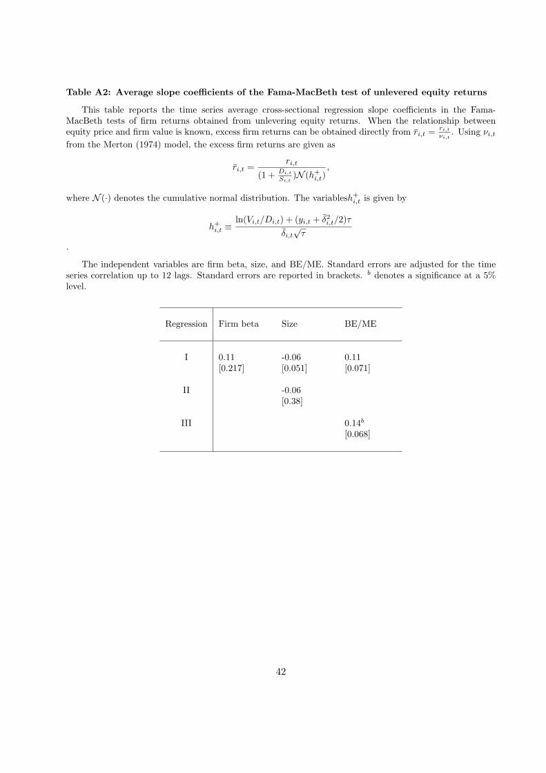
Table A2: Average slope coefficients of the Fama-MacBeth test of unlevered equity returns

This table reports the time series average cross-sectional regression slope coefficients in the Fama-MacBeth tests of firm returns obtained from unlevering equity returns. When the relationship betweenequity price and firm value is known, excess firm returns can be obtained directly from r̄i,t = ri,t

νi,t. Using νi,t

from the Merton (1974) model, the excess firm returns are given as

r̄i,t =ri,t

(1 + Di,t

Si,t)N (h+

i,t),

where N (·) denotes the cumulative normal distribution. The variablesh+i,t is given by

h+i,t ≡

ln(Vi,t/Di,t) + (yi,t + δ̄2i,t/2)τδ̄i,t√τ

.

The independent variables are firm beta, size, and BE/ME. Standard errors are adjusted for the timeseries correlation up to 12 lags. Standard errors are reported in brackets. b denotes a significance at a 5%level.

Regression Firm beta Size BE/ME

I 0.11 -0.06 0.11[0.217] [0.051] [0.071]

II -0.06[0.38]

III 0.14b

[0.068]

42

The Role of Capital Structure in Cross-Sectional...

Documents

Transcript of The Role of Capital Structure in Cross-Sectional...