The RKFIT algorithm for nonlinear rational Berljafa, …eprints.ma.man.ac.uk/2309/01/main.pdfThe...

The RKFIT algorithm for nonlinear rationalapproximation

Berljafa, Mario and Güttel, Stefan

2015

MIMS EPrint: 2015.38

Manchester Institute for Mathematical SciencesSchool of Mathematics

The University of Manchester

Reports available from: http://eprints.maths.manchester.ac.uk/And by contacting: The MIMS Secretary

School of Mathematics

The University of Manchester

Manchester, M13 9PL, UK

ISSN 1749-9097

http://eprints.maths.manchester.ac.uk/

THE RKFIT ALGORITHM FOR NONLINEARRATIONAL APPROXIMATION

MARIO BERLJAFA∗

AND STEFAN GUTTEL∗

Dedicated to the memory of Axel Ruhe (1942–2015)

Abstract. The RKFIT algorithm outlined in [M. Berljafa and S. Guttel, Generalizedrational Krylov decompositions with an application to rational approximation, SIAM J. MatrixAnal. Appl., 2015] is a Krylov-based approach for solving nonlinear rational least squares prob-lems. This paper puts RKFIT into a general framework, allowing for its extension to nondiagonalrational approximants and a family of approximants sharing a common denominator. Furthermore,we derive a strategy for the degree reduction of the approximants, as well as methods for their conver-sion to partial fraction form, for the efficient evaluation, and root-finding. We also discuss commonsand differences of RKFIT and the popular vector fitting algorithm. A MATLAB implementation ofRKFIT is provided and numerical experiments, including the fitting of a MIMO dynamical systemand an optimization problem related to exponential integration, demonstrate its applicability.

Key words. nonlinear rational approximation, least squares, rational Krylov method

AMS subject classifications. 15A22, 65F15, 65F18, 30E10

1. Introduction. Rational approximation problems arise in many areas of engi-neering and scientific computing. A prominent example is that of system identificationand model order reduction, where calculated or measured frequency responses of dy-namical systems are approximated by (low-order) rational functions [18, 24, 2, 21, 17].Some other areas where rational approximants play an important role are analoguefilter design [6], time-stepping methods [41], transparent boundary conditions [27],and iterative methods in numerical linear algebra (see, e.g., [31, 40, 16, 25, 32]). Herewe focus on discrete rational approximation in the least squares (LS) sense.

In its simplest form the weighted rational LS problem is the following: givendata pairs {(λi, fi)}Ni=1, with pairwise distinct λi, and positive weights {wi}Ni=1, finda rational function r of type (m,m), that is, numerator and denominator of degree atmost m, such that

N∑i=1

wi|fi − r(λi)|2 → min. (1.1)

The weights can be used to assign varying relevance to the data points. For example,when the function values fi are known to be perturbed by white Gaussian noise, thenthe wi can be chosen inversely proportional to the variance.

Even in their simplest form (1.1), rational LS problems are challenging. Finding arational function r = pm/qm in (1.1) corresponds to a nonlinear minimization problemas the denominator qm is generally unknown, and solutions may depend discontin-uously on the data, be non-unique, or even non-existent. An illustrating exampleinspired by Braess [9, p. 109] is to take fixed m ≥ 1 and N > 2m, and let

λi =i− 1N

, and fi =

{1 if i = 1,0 if 2 ≤ i ≤ N. (1.2)

∗School of Mathematics, The University of Manchester, Alan Turing Building, Ox-

ford Road, M13 9PL Manchester, United Kingdom, [email protected],[email protected]

1

2 M. BERLJAFA AND S. GUTTEL

Then the sequence of rational functions rj(z) = 1/(1 + jz) makes the misfit for (1.1)arbitrarily small as j → ∞, but the fi do not correspond to values of a type (m,m)rational function (there are too many roots). Hence a rational LS solution does notexist. If, however, the data fi are slightly perturbed to fi = rj(λi) for an arbitrarilylarge j, then of course rj itself is a LS solution to (1.1).

A very common approach for solving (1.1) approximately is linearisation. Con-sider again the data (1.2) and the problem of finding polynomials pm and qm of degreeat most m such that

N∑i=1

wi|fiqm(λi)− pm(λi)|2 → min. (1.3)

This problem has a trivial solution with qm ≡ 0 and to exclude it we need some nor-malisation like, for example, a “point-wise” condition qm(0) = 1. Under this conditionthe linear problem (1.3) is guaranteed to have a nontrivial solution (pm, qm), but thesolution is clearly not unique; since fi = 0 for i ≥ 2, any admissible denominator poly-nomial qm with qm(0) = 1 corresponds to a minimal solution with pm 6≡ 0. On theother hand, for the normalisation condition qm(1) = 1, the polynomials qm(z) = z andpm ≡ 0 solve (1.3) with zero misfit. This example shows that linearised rational LSproblems can have non-unique solutions, and these may depend on normalisation con-ditions. With both normalisation conditions, the rational function r = pm/qm with(pm, qm) obtained from solving the linearised problem (1.3) may yield an arbitrarilylarge (or even infinite) misfit for the nonlinear problem (1.1).

The pitfalls of nonlinear and linearised rational approximation problems have notprevented the development of algorithms for their solution. An interesting overviewof algorithms for the nonlinear problem based on repeated linearisation, such asWittmeyer’s algorithm, is given in [3]. Robust solution methods for the linearisedproblem using regularised SVD are discussed in [20, 19].

The aim of this paper is to present and analyse an extension of the RKFITalgorithm initially outlined in [5]. RKFIT is an iterative method for solving rationalLS problems more general than (1.1). In its original form, for given matrices {A,F} ⊂CN×N and a vector b ∈ CN , RKFIT attempts to find a rational function r of type(m,m) such that

‖Fb − r(A)b‖22 → min. (1.4)

Note that this problem contains (1.1) as a special case with F = diag(fi), A =diag(λi), and b = [

√w1 . . .

√wN ]T . For RKFIT the matrices A and F are not

required to be diagonal. In many applications F is a matrix function of A or anapproximation thereof, i.e., F = f(A) or F ≈ f(A).

Here we extend RKFIT to approximation problems involving a family of matrices{F [j]}`j=1 ⊂ CN×N , a block of vectors B = [b1 . . . bn] ∈ CN×n, and rationalfunctions of type (m+k,m) with k not necessarily being equal to zero. More precisely,we seek a family of rational functions {r[j]}`j=1 of type (m+k,m), all sharing a commondenominator qm, such that the relative misfit is minimal, i.e.,

misfit =

√√√√∑`j=1 ‖D[j][F [j]B − r[j](A)B]‖2F∑`

j=1 ‖D[j]F [j]B‖2F→ min. (1.5)

THE RKFIT ALGORITHM 3

The matrices F [j] may, for instance, correspond to values of a parameter-dependentmatrix function like F [j] = exp(−tjA), and in section 6 we consider applications ofsuch approximation problems. The matrices D[j] act as element-wise weights, whereasthe vectors in B can be viewed as spectral weights relative to the eigenpairs of A.

To summarize our terminology, here is a list of the data in problem (1.5):

A : interpolation node matrix of size N ×N ,F [j] : interpolation data matrices of size N ×N ,D[j] : element-wise weight matrices of size N ×N ,B : block of spectral weight vectors, an N × n matrix,r[j] : rational functions sharing the same denominator qm,

(m+ k,m) : approximation type of the functions r[j], with k ≥ −m.

We show how rational Krylov techniques can be used to tackle problems of theform (1.5). The outgrowth of this work is a new MATLAB implementation of RKFIT,which is part of the Rational Krylov Toolbox [4] available online1. One particularityof RKFIT is its ease of use. For example, with ` = 1 and the matrices A, F, B and avector of initial poles xi being defined in MATLAB, the user simply calls

[xi, misfit, ratfun] = rkfit(F, A, B, xi);

to obtain a rational function r represented as a MATLAB object ratfun. The tool-box implements several methods for ratfun, for example, the evaluation of r at scalararguments or as a matrix function; the commands ratfun(z) and ratfun(A,B) eval-uate r(z) and r(A)B, respectively (where A and B need not be the same matrices asused for the construction of ratfun). The conversion of a ratfun to partial fractionform (the residue command), root-finding (roots), or easy-to-use plotting (ezplot)are provided as well. The use of MATLAB’s object-oriented programming capabilitiesfor these purposes is inspired by the Chebfun system [13].

Alongside with the extension of RKFIT from (1.4) to (1.5), another contributionof this paper is Theorem 3.1 and its Corollary 3.2, showing that RKFIT solves (1.5)exactly if the F [j] are rational matrix functions of type (m + k,m). Further, insection 4, we propose an automated procedure for decreasing the degree parameters mand k, thereby reducing possible deficiencies in the rational approximants. In section 5we develop a new approach for the efficient evaluation of the rational approximants(and their derivatives) produced by RKFIT. We also show how to compute the roots ofthese approximants, or convert them into partial fraction form. Numerical examplesare given in section 6, including the fitting of a MIMO dynamical system and a newpole optimization approach for exponential integration. An appendix discusses theconnections of RKFIT and other approximation algorithms, in particular, the popularvector fitting method [24].

We note that initially we consider the case n = 1, i.e., B = b ∈ CN is a singlevector. This is merely for simplicity of exposition, and the extension to the block-casen ≥ 1 is given in section 3.5.

2. Preliminaries. Our derivation of RKFIT relies on rational Krylov spacesand in this section we review the required facts and introduce notation.

1http://guettel.com/rktoolbox/


2.1. Rational Krylov spaces. Given a matrix A ∈ CN×N , a (so-called) start-ing vector b ∈ CN , an integer m ≥ 0, and a nonzero polynomial qm ∈ Pm with rootsdisjoint from the spectrum of A, we define the associated rational Krylov space as

Qm+1 ≡ Qm+1(A, b, qm) := qm(A)−1Km+1(A, b),

where Km+1 ≡ Km+1(A, b) := span{b, Ab, . . . , Amb} is a polynomial Krylov space.There exists an integer M(A, b) ≡ M ≤ N , called the invariance index for (A, b),such that K1 ⊂ K2 ⊂ · · · ⊂ KM−1 ⊂ KM = KM+1. Throughout this work weassume that m < M , in which case both Km+1(A, b) and Qm+1(A, b, qm) are of fulldimension m+ 1. As a consequence, each vector v ∈ Qm+1(A, b, qm) corresponds toa unique rational function r = pm/qm of type (m,m) such that v = r(A)b, and viceversa. We denote this correspondence by r ≡ v .

The roots of qm are called poles of the rational Krylov space and denoted byξ1, ξ2, . . . , ξm. We often refer to qm itself as poles of the rational Krylov space. Ifdeg(qm) < m, then m − deg(qm) of the poles are set to ∞, and we refer to them asformal (multiple) roots of qm.

2.2. The rational Krylov method. The rational Krylov method [34, 35, 36,37] constructs an orthonormal basis Vm+1 ∈ CN×(m+1) of Qm+1(A, b, qm) by applyingthe Gram–Schmidt process to {b, p1(A)q1(A)−1b, . . . , pm(A)qm(A)−1b}, with qj(z) =∏j

i=1ξi 6=∞

(z − ξi) and some nonzero polynomials pj ∈ Pj . The method is listed in

Algorithm 2.1. It computes a decomposition of the form

AVm+1Km = Vm+1Hm, (2.1)

where (Hm,Km) is an (m + 1) × m upper-Hessenberg pencil satisfying |hj+1,j | +|kj+1,j | 6= 0 and ξj = hj+1,j/kj+1,j /∈ Λ(A) for j = 1, . . . ,m. Any such decompositionis called a rational Arnoldi decomposition (RAD), see [5, Definition 2.3]. Further,the numbers hj+1,j/kj+1,j are called the poles of the pencil (Hm,Km). With anyrational Krylov space Qm+1 ≡ Qm+1(A, b, qm) we can associate a RAD (2.1) suchthat R(Vm+1) = Qm+1, v1 is collinear to b, and the poles of (Hm,Km) are the(formal) roots of qm. Here, R(Vm+1) denotes the range of Vm+1. In this sense we saythat (2.1) is a RAD for Qm+1.

Algorithm 2.1 Rational Krylov method [34, 36, 37]. RK Toolbox [4]: rat krylov

Input: A ∈ CN×N , b ∈ CN , and poles {ξj}mj=1 ⊂ C \ Λ(A) with m < M(A, b).Output: Decomposition (2.1).

1. For every j = 1, . . . ,m, take any (νj , µj , ρj , ηj) satisfying (2.3).2. Set v1 := b/‖b‖2.3. for j = 1, . . . ,m do4. Choose nonzero tj ∈ Cj . See discussion following (2.2).5. Compute w := (νjA− µjI)−1(ρjA− ηjI)Vjtj .6. Project yj := V ∗j w and compute yj+1,j := ‖w − Vjyj‖2.7. Compute vj+1 := (w − Vjyj)/yj+1,j orthogonal to v1, . . . , vj .8. Set kj := νjyj − ρjtj and hj := µjyj − ηjtj , where tj = [tTj 0]T . See (2.2).9. end for


Let us discuss briefly the choice of the parameters in Algorithm 2.1. From lines5–8 we retrieve (for j = 1, . . . ,m)

Vj+1yj = (νjA− µjI)−1(ρjA− ηjI)Vjtj , (2.2a)

AVj+1

(νjyj − ρjtj

)= Vj+1

(µjyj − ηjtj

), (2.2b)

AVj+1kj = Vj+1hj . (2.2c)

The vector tj ∈ Cj is called continuation combination as Vjtj is used to expand thespace. For tj we use a unit 2-norm left null vector of µjKj−1 − νjHj−1 if j > 1, andt1 = e1 if j = 1, as proposed in [37]. This left null vector is unique, up to scaling, asµjKj−1 − νjHj−1 is of full column rank [5, Section 2].

To handle both finite and infinite poles {ξj}mj=1 in a unified way, we introduce foreach j the quadruple (νj , µj , ρj , ηj) ∈ C4 such that

µj/νj = ξj and ρjµj 6= ηjνj . (2.3)

The first property assures that we build a rational Krylov space having the poles{ξj}mj=1, cf. (2.2a), while the second forbids a deficient case where (νjA−µjI)−1(ρjA−ηjI) is a scalar multiple of the identity matrix. Our choice is (νj , µj) = (1, ξj) forfinite ξj , and (νj , µj) = (0, 1) when ξj = ∞, whilst (ρj , ηj) = (0, 1) for |ξj | < 1 and(ρj , ηj) = (1, 0) otherwise.

Collecting the vectors kj , appropriately padded with zeros to be of size m+ 1, ina matrix Km and accordingly for Hm, we arrive at the decomposition (2.1).

3. The RKFIT algorithm. The RKFIT algorithm aims to find rational func-tions {r[j]}`j=1 of type (m + k,m), all sharing a common denominator qm ∈ Pm,solving problem (1.5). As the denominator qm is not known and hence (1.5) is nonlin-ear, RKFIT tries to iteratively improve a starting guess for qm by solving a linearisedproblem at each iteration.

RKFIT is succinctly described in Algorithm 3.2. Different from the basic versionpresented in [5], our new description of RKFIT makes use of two linear spaces in CN ,a search space S and a target space T , both of which are (rational) Krylov spaces.By PT we denote the orthogonal projection onto T . The essence of Algorithm 3.2 isthe relocation of poles in line 7. Since with any polynomial qm ∈ Pm we can associatea vector v = qm(A)qm(A)−1b ∈ S, and the other way around, we may identify qm,the improvement of qm, by looking for the corresponding vector v ∈ S. This is indeeddone in line 5 and further explained in Section 3.2. Corollary 3.2, a consequence ofthe following Theorem 3.1, provides insight into the RFFIT pole relocation, i.e., lines5–7 in Algorithm 3.2. We use ` = 1 and D[1] = I for simplicity only. The result easilyextends to ` > 1 and arbitrary nonsingular D[j].

Theorem 3.1. Let qm, q?m ∈ Pm be nonzero polynomials with roots disjoint from

the spectrum of A ∈ CN×N . Fix −m ≤ k ∈ Z, and let b ∈ CN be such that 2m+ k <M(A, b). Assume that F = p?m+k(A)q?m(A)−1 for some p?m+k ∈ Pm+k. Define S andT as in lines 3 and 4 of Algorithm 3.2, respectively, and let Vm+1 be an orthonormalbasis of S. The matrix (I − PT )FVm+1 has a nullspace of dimension ∆m+ 1 if andonly if ∆m is the largest integer such that p?m+k/q

?m is of type (m+k−∆m,m−∆m).

Proof. Let v = pm(A)qm(A)−1b ∈ S, with pm ∈ Pm being arbitrary. Then

F v = p?m+k(A)q?m(A)−1pm(A)qm(A)−1b =: p2m+k(A)q?m(A)−1qm(A)−1b


Algorithm 3.2 High-level description of RKFIT. RK Toolbox [4]: rkfit1. Take initial guess for qm.2. repeat3. Set search space S := Qm+1(A, b, qm). See section 2.4. Set target space T := Km+k+1(A, qm(A)−1b). See section 3.1.5. Find v = argmin v∈S

‖v‖2=1

∑`j=1 ‖D[j] (I − PT )F [j]v‖22. See section 3.2.

6. Let qm ∈ Pm be such that v = qm(A)qm(A)−1b. See section 3.2.7. Set qm := qm. See Corollary 3.2.8. until stopping criteria is satisfied. See sections 3.2–3.3.9. Construct wanted approximants {r[j]}`j=1. See section 3.3.

has a unique representation in terms of p2m+k/(q?mqm) since 2m+k < M . Assume that

F v ∈ T . In this case we also have the representation F v = pm+k(A)qm(A)−1b, with auniquely determined pm+k ∈ Pm+k. By the uniqueness of the rational representationswe conclude that p2m+k/(q

?mqm) = pm+k/qm, or equivalently, q?m|p2m+k = pm+kpm.

Hence, the poles of pm+k−∆m/q?m−∆m = pm+k/q

?m must be roots of pm. The other

∆m roots of pm can be chosen freely, giving rise to the (∆m+1)-dimensional subspace

N :={p∆m(A)q?m−∆m(A)qm(A)−1b

∣∣∣ p∆m ∈ P∆m

}⊆ S, (3.1)

whose elements v are such that F v ∈ T . Hence, ∆m + 1 is the dimension of thenullspace of (I − PT )FVm+1.

Corollary 3.2. Let qm, q?m, F,A, b,m, k,S, and T be as in Theorem 3.1. Then

p?m+k and q?m are coprime and either deg(p?m+k) = m+ k or deg(q?m) = m if and onlyif there is a unique, up to unimodular scaling, solution to ‖ (I − PT )F v‖22 → min,over all v ∈ S of unit 2-norm. This solution is given by v = γq?m(A)qm(A)−1b withsome scaling factor γ ∈ C.

The corollary asserts that if Fb = pm+k(A)q?m(A)−1b and ∆m = 0, then the“roots” of v = γq?m(A)qm(A)−1b match the unknown poles q?m and the next approx-imate poles become qm := q?m. Hence RKFIT identifies the exact poles within oneiteration independently of the starting guess qm. If ∆m > 0 the exact m−∆m polesare also found, but additional ∆m superfluous poles at arbitrary locations are presentas well. Based on Theorem 3.1 we develop in section 4 an automatic procedure to re-duce the denominator degree m by ∆m, and adapt k. When dealing with noisy data(and roundoff) or when Fb cannot be exactly represented as r(A)b for a rationalfunction r of type (m+ k,m), the convergence of RKFIT is not understood.

In the remaining part of this section we show how the various parts of Algo-rithm 3.2 are realized using rational Krylov techniques.

3.1. Constructing the target space. We assume (2.1) has been constructed.Hence for the search space we have S = R(Vm+1). If k = 0, then S = T andPT = Vm+1V

∗m+1. Otherwise S either has to be expanded (if k > 0) or compressed

(if k < 0) to get T .Let us first consider superdiagonal approximants, i.e., k > 0. In this case T =

Qm+k+1(A, b, qm), the rational Krylov space of dimension m + k + 1 with m polesbeing the roots of qm and additional k poles at infinity. In order to get an orthonormalbasis for Qm+k+1(A, b, qm), we expand (2.1) to AVm+k+1Km+k = Vm+k+1Hm+k byperforming k additional polynomial steps with the rational Krylov method. Let us,


for convenience, label by Vm+k+1 := Vm+k+1 the orthonormal basis for T when k ≥ 0.Thus, PT = Vm+k+1V

∗m+k+1.

We now consider the subdiagonal case k < 0. The target space T is givenby T = Km+k+1(A, qm(A)−1b). Note that Qm+1(A, b, qm) = Km+1(A, qm(A)−1b).Therefore, we aim at transforming the RAD (2.1) for Qm+1(A, b, qm) into a RAD

AVm+1Km = Vm+1Hm, (3.2)

for Km+1(A, qm(A)−1b). An orthonormal basis for T is then given by truncatingVm+1 to Vm+k+1, the first m+ k + 1 columns of Vm+1.

Using a sequence of Givens rotations in a QZ fashion (as explained in [38, p. 495])we get unitary Qm+1 ∈ C(m+1)×(m+1) and Zm ∈ Cm×m such that Km = Q∗m+1KmZmis upper-triangular and Hm = Q∗m+1HmZm is upper-Hessenberg. Fittingly, the poleshj+1,j/kj+1,j of (3.2), where Vm+1 = Vm+1Qm+1, are all at infinity. Hence R(Vj+1) =Kj+1(A, qm(A)−1b) for j = 0, 1, . . . ,m, and we can set PT = Vm+k+1V

∗m+k+1.

3.2. Solving the linear problem and relocating poles. We consider theproblem in line 5 of Algorithm 3.2, i.e., the problem of finding a unit 2-norm vectorv ∈ S such that

∑`j=1 ‖D[j] (I − PT )F [j]v‖22 is minimal. We have S = R(Vm+1) and

T = R(Vm+k+1) with both Vm+1 and Vm+k+1 being orthonormal.Defining the matrix S = [ST1 . . . ST` ]T ∈ CN`×(m+1), where

Sj = D[j][F [j]Vm+1 − Vm+k+1

(V ∗m+k+1F

[j]Vm+1

)]∈ CN×(m+1), (3.3)

a solution is given by v = Vm+1c, where c is a right singular vector of S correspondingto a smallest singular value σmin.

We now show how to determine the polynomial qm ∈ Pm, from line 6 of Algo-rithm 3.2, such that v = Vm+1c = qm(A)qm(A)−1b. As this part is independent of k,the procedure is the one presented in [5, Section 5], and we review it only briefly.

Let Qm+1 ∈ C(m+1)×(m+1) be unitary with first column Qm+1e1 = c. Using(2.1) as a RAD for S, it follows from [5, Theorem 4.4] that the roots of qm are theeigenvalues of the m×m pencil([

0 Im]Q∗m+1Hm,

[0 Im

]Q∗m+1Km

). (3.4)

Note that if c = e1, the first canonical unit vector, then v is collinear with b. In thiscase qm and qm share the same roots and the algorithm stagnates.

3.3. Constructing the approximants. The approximants {r[j]}`j=1 of type(m + k,m) are computed by LS approximation of F [j]b from the rational Krylovspace Qbm+1(A, b), m = max{m,m + k}, with poles ξ1, . . . , ξm identified by RKFITand max{0, k} poles at ∞. More precisely, let Vbm+1 be an orthonormal basis ofQbm+1(A, b) with associated RAD

AVbm+1Kbm = Vbm+1Hbm. (3.5)

Each r[j] is represented by a coefficient vector c[j] ∈ C bm+1 such that r[j](A)b/‖b‖2 =Vbm+1c

[j]. The coefficient vectors are given by

c[j] =

{V ∗bm+1

(F [j]b

)/‖b‖2 if D[j] = IN ,(

D[j]Vbm+1

)†(D[j]F [j]b

)/‖b‖2 otherwise,

(3.6)


with X† denoting the Moore–Penrose pseudoinverse of X.Computing the coefficients c[j] at each iteration does not significantly increase

the computational complexity because the D[j]F [j]b need to be computed only once.The coefficients c[j] enable the cheap evaluation of the relative misfit (1.5), whichallows to stop the RKFIT iteration when a wanted tolerance εtol is achieved.

3.4. Avoiding complex arithmetic. If F [j], A, and b are real-valued and theset of starting poles {ξj}mj=1 is closed under complex conjugation, we can use the“real version” of Algorithm 2.1, see [35]. The matrices Sj in (3.3) are guaranteed tobe real-valued and the generalized eigenproblem (3.4) is real-valued as well. Apartfrom requiring less memory and making the computation faster, this also guaranteesthe relocated poles to appear in complex-conjugate pairs.

If F [j], A, and b are not real-valued, but can be simultaneously transformed intoreal-valued form, complex arithmetic can be avoided too. We show how to achievethis for scalar data, assuming ` = 1 for simplicity. Let the data set {(λi, fi)}Ni=1 beclosed under complex conjugation, i.e., if (λ, f) is in the set, so is (λ, f). Without lossof generality, we assume that the pairs are ordered such that {(λi, fi)}NR

i=1 ⊂ R2 and{(λi, fi)}Ni=NR+1 ⊂ C2 \ R2, where the complex-conjugate pairs in the latter subsetappear next to each other, and 0 ≤ NR ≤ N is a natural number. Define A =diag(λ1, . . . , λN ), F = diag(f1, . . . , fN ), b = [1 . . . 1]T ∈ RN , and let Q ∈ CN×N

be unitary. Then

‖Fv − r(A)b‖2 = ‖ (QFQ∗) (Qb)−Qr(A)Q∗ (Qb) ‖2= ‖ (QFQ∗) (Qb)− r(QAQ∗) (Qb) ‖2.

The first equality follows from the unitary invariance of the 2-norm, and the secondfrom [26, Theorem 1.13]. With the particular choice

Q = blkdiag

(INR

,

√2

2

[1 1−i i

], . . . ,

√2

2

[1 1−i i

])∈ CN×N ,

we have FR = QFQ∗ ∈ RN×N , AR = QAQ∗ ∈ RN×N and bR = Qb ∈ RN . Precisely,

FR = blkdiag

(f1, . . . , fNR

,

[<(fi1) −=(fi1)=(fi1) <(fi1)

], . . . ,

[<(fiNC

) −=(fiNC)

=(fiNC) <(fiNC

)

]),

where NC = N−NR2 and ij = NR + 2j − 1. For AR we obtain an analogous expression,

while bR = [1 . . . 1√

2 0 . . .√

2 0]T , with NR entries equal to 1, and NC

consecutive [√

2 0]T copies.

3.5. Block case. Let us consider the case B = [b1 . . . bn] ∈ CN×n withn > 1. Introduce the Nn×Nn matrices

D [j] = In ⊗D[j], F [j] = In ⊗ F [j], and A = In ⊗A, (3.7)

where In ⊗X = blkdiag(X, . . . ,X). Since

‖D[j][F [j]B − r[j](A)B]‖2F = ‖D [j][F [j]vec(B)− r[j](A)vec(B)]‖22we recover the single-column case n = 1 considered so far, with b = vec(B).


Our implementation [4] supports the case n > 1, and takes advantage of thestructure present in (3.7) so that only {D[j], F [j]}`j=1 and A are stored, while D [j],F [j],and A are never constructed explicitly. In fact D[j], F [j], and A are not explicitlyneeded either, as all that is required is the ability to compute D[j]x , F [j]x , Ax forarbitrary x ∈ CN , as well as the ability to solve shifted linear systems (A− ξI)x = v .

4. Tuning degree parameters m and k. In some applications, one may wantto construct a rational function of sufficiently small misfit without knowing the re-quired degree parameters m and k in advance. In such situations one can try to fit thedata with high enough (for instance maximal one is willing to use) degree parametersand then, after RKFIT has found a sufficiently good approximant, reduce m and kwithout deteriorating much the approximation accuracy. In this section we present astrategy for performing this reduction.

For ease of notation we consider the case ` = 1, n = 1, and D = I. We assumeto have at hand an (m+ k,m) approximant r such that ‖Fb − r(A)b‖2 ≤ ‖Fb‖2εtol.We then propose the following three-step procedure. (1) Reduce m to m−∆m ≥ 0,with ∆m such that m − ∆m + k ≥ 0. (2) Find lower-degree approximant of type(m − ∆m + k,m − ∆m). (3) Reduce k if required. These steps are discussed inthe following three subsections for the case that F is a rational matrix function. Anillustration is given in Figure 4.1. In subsection 4.4 we discuss the case when F is nota rational matrix function.

4.1. Reducing the denominator degree m. Assume that F is a rationalmatrix function. Our reduction procedure for m is based on Theorem 3.1, whichasserts that a defect ∆m + 1 of the matrix S = (I − PT )FVm+1 corresponds to Fbeing of type (m−∆m+k,m−∆m). Due to numerical roundoff, the numerical rankof S related to a given tolerance ‖Fb‖2εtol (with, e.g., εtol = 10−15) is computed.More precisely, we reduce m by the largest integer ∆m ≤ min{m,m+ k} such that

σm+1−∆m ≤ ‖Fb‖2εtol, (4.1)

where σ1 ≤ · · · ≤ σm+1 are the singular values of S.

4.2. Finding a lower-degree approximant. If ∆m ≥ 1, then m needs tobe reduced and a new approximant of lower numerator and denominator degree isrequired. As seen in the proof of Theorem 3.1, the ∆m+1 linearly independent vectorsspanning N all share as the greatest common divisor (GCD) the polynomial q?m−∆m,and its roots should be used as poles of the reduced-degree rational approximant. Thefollowing theorem shows how these roots can be obtained from the pencil (Hm,Km)in (2.1).

Theorem 4.1. Let (2.1) be a RAD for Qm+1(A, b, qm), with m+ 1 < M(A, b),and let the rj ≡ Vm+1cj for j = 1, . . . ,∆m + 1 be linearly independent. Assumethat the numerators of rj share as GCD a polynomial of degree m − ∆m. Let X ∈C(m+1)×(m+1) be a nonsingular matrix with Xej = cj for j = 1, . . . ,∆m+1. Introduce

K? =[O Im−∆m

]X−1Km

[O

Im−∆m

], H? =

[O Im−∆m

]X−1Hm

[O

Im−∆m

].

Assume further that K? is nonsingular. Then the roots of the GCD are the eigenvaluesof the (m−∆m)× (m−∆m) generalized eigenproblem (H?,K?).

Proof. We transform the RAD (2.1) into AVm+1Km = Vm+1Hm, where Vm+1 =Vm+1X, Km = X−1KmY , and Hm = X−1HmY , and with Y = blkdiag(I∆m,K?)

−1.


Hence in scalar form, for all z ∈ C we have

zr(z)Km = r(z)Hm ⇐⇒ r(z)(zKm − Hm

)= 0T ,

where r(z) = [r1(z) . . . r∆m+1(z) r∆m+2(z) . . . rm+1(z)]. Introduce K? andH? as the lower-right (m − ∆m) × (m − ∆m) submatrices of Km and Hm, respec-tively. Since Λ(H?,K?) = Λ(H?, K?), we need to show that the roots of the GCD areΛ(H?, K?).

Let λ be a common root of {rj}∆m+1j=1 . Then the last m − ∆m columns of

r(λ)(λKm − Hm) = 0T assert that λ is a generalized eigenvalue of (H?, K?) withleft eigenvector r?(λ)∗ = [r∆m+2(λ) . . . rm+1(λ)]∗ 6= 0. This handles simple roots.

Let us now assume that λ is a root of multiplicity 2. Note that K? = Im−∆m.Differentiating the scalar RAD with respect to λ gives

r ′(λ)(λKm − Hm

)+ r(λ)Km = 0T ⇐⇒ r ′(λ)

(λKm − Hm

)= −r(λ)Km.

The last m−∆m columns in the latter relation give

r ′?(λ)(λK? − H?

)= −r?(λ)K? = −r?(λ) 6= 0T .

In particular r ′?(λ) 6= 0T . Further r ′?(λ)(λK? − H?

)2 = −r?(λ)(λK? − H?

)= 0T .

Hence r ′?(λ) is a generalized eigenvector for the eigenvalue λ of (H?, K?), which ishence of multiplicity two or greater. The proof for roots of higher multiplicity followsthe same argument.

Remark 4.2. The assumption that K? is nonsingular is used in the proof ofTheorem 4.1 for the case of repeated roots only. We conjecture that this assumptioncan be removed also when there are multiple roots, and that it follows from the factthat the numerators of {rj}∆m+1

j=1 have as GCD a polynomial of degree m−∆m.

4.3. Numerator degree revealing basis. We now assume that the denomi-nator degree m := m − ∆m has already been reduced and a new approximant r oftype (m+k,m) such that ‖Fb− r(A)b‖2 ≤ ‖Fb‖2εtol has been found. Reducing thenumerator degree is a linear problem and we can guarantee the misfit to stay belowεtol after the reduction.

Let T = Km+k+1(A, qm(A)−1b) be the final target space such that r(A)b ∈ T ,and let Vj be an orthonormal basis for Kj(A, qm(A)−1b) for j = 1, . . . ,m + k + 1.As the vectors in Vj have ascending numerator degree, this basis reveals the degreeof r(A)b by looking at the trailing expansion coefficients c ∈ Cm+k+1 satisfyingr(A)b/‖b‖2 = Vm+k+1c.

Introduce c−i = [O Ii]c ∈ Ci for i = 1, . . . ,m+ k. By the triangle inequality,∥∥∥Fb/‖b‖2 − Vm+k+1c + Vm+k+1

[0

c−i

] ∥∥∥2≤∥∥∥Fb/‖b‖2 − Vm+k+1c

∥∥∥2

+∥∥∥ [ 0

c−i

] ∥∥∥2.

The degree of the numerator of r can therefore be reduced to m+ k−∆k, where ∆kis the maximal integer 1 ≤ i ≤ m+ k such that

‖c−i‖2 ≤ ‖Fb‖2εtol − ‖Fb − r(A)b‖2, (4.2)

or ∆k = 0 if such an integer i does not exist. The last ∆k components of c mayhence be truncated, giving c ∈ Cm+k−∆k+1 such that r ≡ Vm+k−∆k+1c still satisfies‖Fb − r(A)b‖2 ≤ ‖Fb‖2εtol.


0 1 2 3 4 5 6 7 8 923456789

m+ k

m

2.5× 10−02

−1.3× 10−03

−4.6× 10−03

6.0× 10−04

4.5× 10−18

1.8× 10−18

︸︷︷︸

cQ

1.9× 10−02

1.7× 10−02

−5.7× 10−17

1.5× 10−17

4.5× 10−18

1.8× 10−18

︸︷︷︸

cK

4

11

1

3

2

567

1Fig. 4.1: Degree reduction when fitting Fb, where F = A(A + I)

−1(A + 3I)

−2, A =

tridiag(−1, 2,−1) ∈ RN×N, and b = e1 ∈ RN

, with N = 150. Note that F is of type(1, 3). The initial poles of the search space are all at infinity. The table on the left shows thenumber ∆m+1 of singular values of (I−PT )FVm+1 below the tolerance ‖Fb‖2εtol = 10

−15,

for different choices of m and k. For the choice (m + k, m) = (3, 9) we obtain ∆m = 2,and hence the reduced type is (1, 7). In this case m is not fully reduced because k was chosentoo small. For the choice (m + k, m) = (8, 6) we obtain ∆m = 3, giving the reduced type(5, 3). The roots of the GCD are −1 and −3 ± i2.32 × 10

−7. With these three poles, and

other two at infinity, the type (5, 3) approximant r produces a relative misfit 7.02 × 10−17

.The expansion coefficients cQ of r in the orthonormal rational basis are given to the rightof the table. They indicate that the last two poles at infinity are actually superfluous, andr is of type at most (3, 3). Only the expansion of r in the orthonormal polynomial basis,as explained in subsection 4.3, reveals that r is of type (1, 3). The coefficients cK in thispolynomial basis are also given.

4.4. General F . The following lemma extends Theorem 3.1 to the case whenF is not necessarily a rational matrix function.

Lemma 4.3. Let qm, A, b,m, k,S, T , and Vm+1 be as in Theorem 3.1. Assumethat for F ∈ CN×N we have found a rational approximant r = pm+k/qm of type(m + k,m) such that ‖Fb − r(A)b‖2 ≤ ‖Fb‖2εtol. If the matrix (I − PT )FVm+1

has ∆m + 1 singular values smaller than ‖Fb‖2εtol, then there exists a (∆m + 1)-dimensional subspace Ng ⊆ S, containing b, such that

minp∈Pm+k

∥∥Fv − p(A)qm(A)−1b∥∥

2≤ ‖Fb‖2εtol

for all v ∈ Ng, ‖v‖2 = 1.Proof. Consider a thin SVD of the matrix (I − PT )FVm+1 = UΣW ∗, where

Σ = diag(σ1, . . . , σm+1) ∈ R(m+1)×(m+1) and σm+1 ≤ · · · ≤ σm−∆m ≤ ‖Fb‖2εtol byassumption. Equivalently, (I − PT )FVm+1W = UΣ. Then the final ∆m+ 1 columnsof Vm+1W form a basis for Ng. It follows from the assumption ‖Fb − r(A)b‖2 ≤‖Fb‖2εtol that b ∈ Ng.

Recall that if F is a rational matrix function, then the space Ng defined inLemma 4.3 corresponds to the exact nullspace N = K∆m+1(A, q?m−∆m(A)qm(A)−1b)defined in (3.1), where the (numerators of the) rational functions share as GCD thepolynomial q?m−∆m. In the general case Ng is only a subspace of the larger rationalKrylov space S, and the rational functions present in Ng do not necessarily share


3 4 5 6 7 8 9 10 11 12234567891011

m+ k

m

11

12

34

4

4

5

5678

1

3 4 5 6 7 8 9 10 11 12234567891011

m+ k

m 00000

000000

0000000

0000101

0000010

0000001

0000000

1Fig. 4.2: Degree reduction when fitting Fb, where F =

pA + A

2, A = tridiag(−1, 2,−1) ∈

RN×N, and b = e1 ∈ RN

, with N = 150. The poles of the search space are obtainedafter three RKFIT iterations with initial poles all at infinity. The table on the left showsthe number ∆m + 1 of singular values of (I − PT )FVm+1 below ‖Fb‖2εtolεsafe = 10

−5for

different choices of m and k. For the choice (m + k, m) = (9, 10) we obtain ∆m = 4,implying the reduced type (5, 6). The choice (m + k, m) = (11, 6) is reduced down to (9, 4) as∆m = 2. Representing this new approximant in the numerator degree-revealing basis allowsfor a further reduction to type (5, 4). The table on the right visualizes how many RKFITiterations are required after reduction to reobtain an approximant of misfit below εtol = 10

−4,

using the approximate GCD strategy for selecting the poles to restart RKFIT with.

a common denominator. However, for every v = pm(A)qm(A)−1b ∈ Ng the vectorFpm(A)qm(A)−1b is well approximated in the 2-norm by some vector p(A)qm(A)−1b,with p ∈ Pm+k. This suggests that the polynomials pm corresponding to vectorsv ∈ Ng share an approximate GCD (see, e.g., [7]) whose roots approximate the polesof a “good” rational approximation r(A)b for Fb. We therefore propose to use thesame reduction procedure as suggested by Theorem 4.1.

As there is no guarantee that after reduction RKFIT will be able to find anapproximant of relative misfit below εtol, the use of a safety parameter εsafe is rec-ommended. More precisely, we reduce m by the largest integer ∆m ≤ min{m,m+k}such that

σm+1−∆m ≤ ‖Fb‖2εtolεsafe, (4.3)

where σ1 ≤ · · · ≤ σm+1 are the singular values of S. By default we use εsafe = 0.1.Figure 4.2 illustrates our reduction strategy for a non-rational function F .

5. Working with rational functions in pencil form. After the RKFIT al-gorithm has terminated, a rational function r of type (m + k,m) is represented bythe pencil (Hbm,Kbm), m = max{m,m + k}, satisfying (3.5) and the coefficients c in(3.6). We now show how to perform computations with this representation.

5.1. Evaluating the approximants and their derivatives. Our approachto evaluating a rational function r is based on the scalar form of (3.5), that is

z[r1(z) . . . rbm+1(z)]Kbm = [r1(z) . . . rbm+1(z)]Hbm,


Algorithm 5.3 Rerunning the rational Krylov method. RK Toolbox [4]: rat krylov

Input: A ∈ C bN× bN , b ∈ C bN , and an upper-Hessenberg pencil (Hbm,Kbm).

Output: Wbm+1 ∈ C bN×( bm+1) such that AWbm+1Kbm = Wbm+1Hbm and Wbm+1e1 = b.

1. for j = 1, . . . , m do2. Define ξj := hj+1,j/kj+1,j , and take any (νj , µj , ρj , ηj) satisfying (2.3).3. Set tj := µjkj − νjhj ∈ Cj , and yj := ηjkj − ρjhj ∈ Cj+1. See (2.2b), (2.2c).

4. Compute w := (νjA− µjI)−1(ρjA− ηjI)Wjtj .5. Compute wj+1 := (w −Wjyj)/yj+1,j .6. end for

with the rational functions rj satisfying rj(A)b/‖b‖2 = vj for all columns vj of Vbm+1.

Given a matrix A ∈ C bN× bN and a starting vector b = w1 ∈ C bN , one easily verifiesthat the vectors wj = rj(A)b satisfy the Arnoldi-type relation

AWbm+1Kbm = Wbm+1Hbm, (5.1)

provided that all rj(A) are defined, i.e., Λ(A) does not contain any of the polesξ1, . . . , ξm. By rerunning the rational Krylov method, we can therefore evaluate eachrational basis function rj(A)b for any matrix argument A and vector b.

Recalling that r(z) =∑bm+1j=1 cjrj(z) with the coefficients c = [cj ] defined in

(3.6), we readily evaluate r(A)b =∑bm+1j=1 cjrj(A)b. In particular, choosing A =

diag(λ1, . . . , λ bN ) and b = [1 . . . 1]T , we can evaluate r pointwise as r(A)b =[r(λ1) . . . r(λ eN )]T . Derivatives of r can easily be evaluated by using a Jordanblock for A. For example, if A = [ λ 1

0 λ ] and b = [0 1]T , then r(A)b = [r′(λ) r(λ)]T .Our method for rerunning the rational Krylov method and thereby generating

(5.1) is given in Algorithm 5.3 and implemented in the rat krylov function of theRational Krylov Toolbox [4].

5.2. Root-finding. For finding the roots of r we recall that r(A)b/‖b‖2 =Vbm+1c = pbm(A)qm(A)−1b. Let us assume that c 6= e1, otherwise r(A)b = c1b, i.e., rhas no roots. Define P = Im+1 − 2uu∗, where u = (γc − e1)/‖γc − e1‖2 and γ ∈ Cis a unimodular scalar such that γe∗1c is real and nonnegative. It follows from [5,Theorem 4.4] that the roots of pbm are the eigenvalues of the m× m pencil([

0 Ibm]PHbm, [0 Ibm]PKbm) .If k < 0, then among the m eigenvalues there are −k infinite eigenvalues, or numer-ically, eigenvalues of large modulus. In our implementation roots of the RationalKrylov Toolbox [4] we hence sort the roots by their magnitudes and return only them+ k smallest ones.

5.3. Conversion to partial fraction form. The conversion of a type (m +k,m) rational function r into partial fraction form can be achieved by transformingthe rational Arnoldi decomposition (3.5) in such a way that it reveals the residues.Here we only consider the case k ≤ 0, i.e., m = m, and pairwise distinct finite poles


Algorithm 5.4 Conversion to partial fraction form. RK Toolbox [4]: residueInput: Upper-Hessenberg pencil (Hm,Km) with finite distinct poles.Output: Invertible matrices Lm+1 and Rm representing the conversion.

1. Set Rm = ([0 Im]Km)−1, Hm := HmRm, and Km := KmRm.2. Set unitary Lm+1 = blkdiag(1, Q∗m), where [0 Im]HmQm = Qmdiag(ξ1, . . . , ξm).3. Update Rm := RmQm, Hm := Lm+1HmQm, and Km := Lm+1KmQm.4. Introduce Dm+1 = [−e1 Km].5. Update Lm+1 := Dm+1Lm+1, Hm := Dm+1Hm, and Km := Dm+1Km.6. Update Rm := RmDm, Hm := HmDm, Km := KmDm, where Dm = diag(1/h1j).7. Redefine Dm := diag(1/kj+1,j), and Dm+1 := blkdiag(1, Dm).8. Update Lm+1 := Dm+1Lm+1, Hm := Dm+1Hm, and Km := Dm+1Km.

ξ1, . . . , ξm (generalizations are discussed in section 7). We aim to transform (3.5) into

AWm+1

01

1. . .

1

= Wm+1

1 1 · · · 1ξ1

ξ2. . .

ξm

, (5.2)

where Wm+1e1 = v1. One then easily verifies that the columns of Wm+1 satisfywj+1 = (A− ξj)−1v1. This conversion is achieved via left- and right-multiplication ofthe pencil (Hm,Km) by invertible matrices as indicated in Algorithm 5.4.

The algorithm consists of four parts. The first corresponds to lines 1–3, andit transforms the pencil so that the lower m × m part matches that of (5.2). Thematrix [0 Im]Km is invertible since it is upper-triangular with no zero elements onthe diagonal (there are no infinite poles), and hence Rm is well defined in line 1. Thesecond part corresponds to lines 4–5, and it zeroes the first row in Km. The thirdpart, line 6, takes care of the first row in Hm, setting all its elements to one. After thistransformation, as the fourth part, we rescale [0 Im]Km in lines 7–8, to recover Im.

The process corresponds to transforming the original Hm and Km as Hm :=Lm+1HmRm and Km := Lm+1KmRm, and the rational Krylov basis Vm+1 is trans-formed accordingly asWm+1 = Vm+1L

−1m+1. Given a coefficient representation r(A)b =

‖b‖2Vm+1cm+1 in the basis Vm+1, we arrive at the partial fraction expansion

r(A)b = ‖b‖Wm+1dm+1 = d0b +m∑j=1

dj(A− ξjI)−1b,

with residues dm+1 = Lm+1cm+1 = [d0 d1 . . . dm]T .The transformation of Vm+1 to the partial fraction basis Wm+1 has condition

number cond(Lm+1), which can be arbitrarily bad in particular if some of the polesξj are close together. Our implementation residue in the Rational Krylov Toolbox [4]therefore supports the use of MATLAB’s variable precision arithmetic as well as theuse of the Advanpix Multiprecision Toolbox [1].

6. Numerical experiments. In the following we demonstrate RKFIT with nu-merical experiments. MATLAB files for reproducing these experiments are part ofthe Rational Krylov Toolbox [4], among other examples (including those in [5]).


6.1. MIMO dynamical system. We consider a model for the transfer functionof the multiple-input/multiple-output (MIMO) system ISS 1R taken from [10]. Thereare 3 input and 3 output channels, giving ` = 9 functions to be fitted. We useN = 2 × 561 sampling points λj given in [10], appearing in complex-conjugate pairson the range ±i[10−2, 103]. The data are closed under complex conjugation, and hencewe can work with block-diagonal real-valued matrices A and {F [j]}`j=1 as explainedin section 3.4. The magnitudes of the ` = 9 transfer functions to be fitted are plottedin Figure 6.1(a).

For the first experiment we try to find rational functions of type (70, 70), andthen reducing their degrees. A tolerance of εtol = 10−3 is used. In Figure 6.1(b) twoconvergence curves are shown, one for RKFIT as described in the previous sections(solid line), and the other for an RKFIT variant that enforces the poles to be stable(dashed line). A pole ξ ∈ C is stable if <(ξ) ≤ 0, and this is enforced in the pole relo-cation step by simply flipping the real parts of the poles if necessary. At convergencethe poles happen to be stable in both cases. The initial poles were taken to be allinfinite, and the misfit at iteration 0 corresponds to these initial poles. Both RKFITvariants achieve a misfit below εtol at iteration 4, after which the degree reductiondiscussed in section 4 takes place. The denominator degree m = 70 is reduced tom − ∆m = 56 without stability enforcement, and to m − ∆ms = 54 with stabilityenforcement. For the latter case, the 70 poles obtained after the fourth iteration andthe 54 poles corresponding to the approximate GCD are plotted in Figure 6.1(c). Theerror corresponding to the new 56 (respectively 54) poles corresponds to iteration 5;as it is still below εtol no further RKFIT iterations are required.

For the second experiment we compare RKFIT with the vector fitting code VFIT[12, 22, 24] for two different choices of initial poles, and with different normalizationconditions for VFIT. (We briefly review VFIT in subsection A.2 of the appendix A.)The results are reported in Figure 6.1(d). Here we search for type (m− 1,m) approx-imants with m = 56, do not enforce the poles to be stable, and do not perform anyfurther degree reductions. The solid convergence curves are obtained with initial polesof the form −ξ/100± iξ, with the ξ being logarithmically spaced on [10−2, 103]. Thisis regarded as a good initial guess in the literature. The dashed curves result whenusing as initial poles the eigenvalues of a a real random matrix. In both cases RKFIToutperforms VFIT, independently of the normalization condition used by VFIT. De-pending on the 56 initial poles, RKFIT requires either 4 or 6 iterations. This has tobe compared to Figure 6.1(b), where the 56 poles selected by our reduction strategyimmediately gave a misfit below εtol so that no further iterations were required. Thisvalidates our approximate GCD strategy for choosing the poles after reducing m.

6.2. Pole optimization for exponential integration. Let us consider theproblem of solving a linear constant-coefficient initial-value problem

Ku ′(t) + Lu(t) = 0, u(0) = u0,

at several time points t1, . . . , t`. Problems like this arise, for example, after space-discretization of parabolic PDEs via finite differences or finite elements, in whichcase K and L are large sparse matrices. Assuming that K is invertible, the exactsolutions u(tj) are given as u(tj) = exp(−tjK−1L)u0, and a popular approach forapproximating u(tj) is to use rational functions r[j] of the form

r[j](z) =σ

[j]1

ξ1 − z+

σ[j]2

ξ2 − z+ · · ·+ σ[j]

m

ξm − z,


10−2 10−1 100 101 102 103

frequency

100

10−3

10−6

10−9

10−12

mag

nit

ud

e

(a) Magnitude of the frequency responses.

0 1 2 3 4 5iteration

100

10−1

10−2

10−3

10−4

mis

fit

RKFIT

RKFIT, stable ξj

εtol

(b) RKFIT with degree reduction.

−10−1 −10−2

real

−60

−30

0

30

60

imag

before reduction

after reduction

(c) Selecting poles during the reduction.

0 2 4 6 8 10 12iteration

100

10−1

10−2

10−3

10−4

mis

fitRKFIT

VFIT

VFIT relaxed

εtol

(d) Comparison between RKFIT and VFIT.

Fig. 6.1: Low-order model approximation to the MIMO system ISS from [10]. The frequencyresponses are plotted in figure (a). In (b) the progress of RKFIT is given for m = 70 infinitestarting poles. At iteration 4 the degree reduction takes place. The 70 poles after convergenceand 54 selected ones (for the case when stability of poles in enforced) are illustrated in figure(c). Figure (d) presents a comparison with VFIT, when searching for (55, 56) approximants,and using two different starting guesses. More details are given in section 6.1.

constructed so that r[j](K−1L)u0 ≈ u(tj). Note that the poles of r[j] do not dependon tj and we have

r[j](K−1L)u0 =m∑i=1

σ[j]i (ξiK − L)−1Ku0,

the evaluation of which amounts to the solution of m decoupled linear systems. Suchfixed-pole approximants have great computational advantage, in particular in combi-nation with direct solvers (the LU factorization of ξiK−L can be used for all tj) andon parallel computers.

The correct design of the pole-residue pairs (ξi, σ[j]i ) is closely related to the

scalar rational approximation of e−tz, a problem which has received considerableattention in the literature [33, 31, 40, 16, 8]. Let us assume that L is Hermitianpositive semi-definite, K is Hermitian positive definite, and define the vector K-norm


as ‖v‖K =√

v∗Kv . Then

‖ exp(−tjK−1L)b − r[j](K−1L)b‖K ≤ ‖b‖K maxλ∈Λ(L,K)

|e−tjλ − r[j](λ)|

≤ ‖b‖K maxλ≥0|e−tjλ − r[j](λ)|, (6.1)

with Λ(L,K) denoting the set of generalized eigenvalues of (L,K).In order to use RKFIT for finding poles ξ1, . . . , ξm of the rational functions r[j]

such that the right-hand side (6.1) of the inequality is small for all j = 1, . . . , `, wepropose a surrogate approach similar to that in [8]. Let A = diag(λ1, . . . , λN ) be adiagonal matrix with “sufficiently dense” eigenvalues on λ ≥ 0. In this example wetake N = 500 logspaced eigenvalues on the interval [10−6, 106]. Further, we define` = 41 logspaced time points tj on the interval [10−1, 101], and the matrices F [j] =exp(−tjA). We also define b = [1 . . . 1]T to assign equal weight to each eigenvalueof A and then run RKFIT for finding a family of type (m − 1,m) rational functionsr[j] with m = 12 so that

absmisfit =∑j=1

‖F [j]b − r[j](A)b‖22

is minimized. Note that

absmisfit ≥∑j=1

‖F [j]b − r[j](A)b‖2∞ =∑j=1

(maxλ∈Λ(A)

|e−tjλ − r[j](λ)|)2

,

and hence a small misfit implies that all r[j] are accurate uniform approximants fore−tjλ on the eigenvalues Λ(A). If these eigenvalues are dense enough on λ ≥ 0 onecan expect the upper error bound (6.1) to be small.

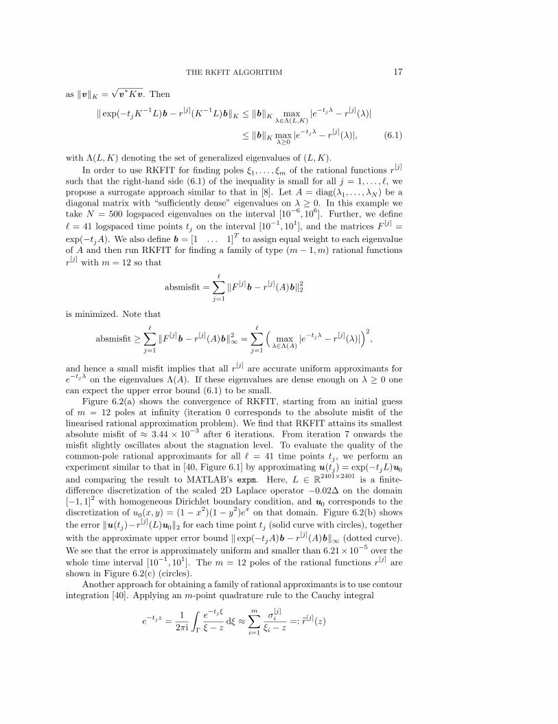
Figure 6.2(a) shows the convergence of RKFIT, starting from an initial guessof m = 12 poles at infinity (iteration 0 corresponds to the absolute misfit of thelinearised rational approximation problem). We find that RKFIT attains its smallestabsolute misfit of ≈ 3.44 × 10−3 after 6 iterations. From iteration 7 onwards themisfit slightly oscillates about the stagnation level. To evaluate the quality of thecommon-pole rational approximants for all ` = 41 time points tj , we perform anexperiment similar to that in [40, Figure 6.1] by approximating u(tj) = exp(−tjL)u0

and comparing the result to MATLAB’s expm. Here, L ∈ R2401×2401 is a finite-difference discretization of the scaled 2D Laplace operator −0.02∆ on the domain[−1, 1]2 with homogeneous Dirichlet boundary condition, and u0 corresponds to thediscretization of u0(x, y) = (1 − x2)(1 − y2)ex on that domain. Figure 6.2(b) showsthe error ‖u(tj)−r[j](L)u0‖2 for each time point tj (solid curve with circles), togetherwith the approximate upper error bound ‖ exp(−tjA)b − r[j](A)b‖∞ (dotted curve).We see that the error is approximately uniform and smaller than 6.21×10−5 over thewhole time interval [10−1, 101]. The m = 12 poles of the rational functions r[j] areshown in Figure 6.2(c) (circles).

Another approach for obtaining a family of rational approximants is to use contourintegration [40]. Applying an m-point quadrature rule to the Cauchy integral

e−tjz =1

2πi

∫Γ

e−tjξ

ξ − z dξ ≈m∑i=1

σ[j]i

ξi − z=: r[j](z)


0 3 6 9 12 15iteration

10−3

10−2

10−1

100

101

102

absm

isfit

RKFIT

(a) Convergence of RKFIT.

10010−1 101

time t

106

103

100

10−3

10−6

erro

r

RKFIT bound

RKFIT

contour

(b) RKFIT vs. the contour approach.

−2 2 6 10 14 180real

−15

−30

0

30

15

imag

RKFIT

contour

(c) Poles from the two approaches.

m error bound

4 5.71× 10−02

7.35× 10−02

8 1.72× 10−03

4.89× 10−03

12 6.21× 10−05

2.47× 10−04

16 5.94× 10−06

1.41× 10−05

20 3.23× 10−07

7.98× 10−07

24 9.53× 10−09

6.62× 10−08

28 4.54× 10−10

4.76× 10−09

32 2.64× 10−11

2.44× 10−10

(d) Quality of RKFIT as m increases.

Fig. 6.2: Approximating exp(−tL)u0 for a range of parameters t with rational approximantssharing common poles. The convergence behaviour of RKFIT, for approximants of type(11, 12), is shown in (a). In (b) we show the approximation error for ` = 41 logspacedtime points t ∈ [0.1, 10] for RKFIT (solid curve with circles) and the contour-based approach(dashed curve with diamonds). The errors of the RKFIT surrogate approximants are alsoindicated (these are approximate upper error bound for the RKFIT approximants). In (c)we show the poles of the two families of rational approximants. The table in (d) shows themaximal RKFIT error and bound, uniformly over all tj, for various m.

on a contour Γ enclosing the positive real axis, one obtains a family of rational func-tions r[j] whose poles are the quadrature points ξi ∈ Γ and whose residuals σ[j]

i dependon tj . As has already been pointed out in [40], such quadrature-based approximantstend be good only for a small range of parameters tj . In Figure 6.2(b) we see thatthe error ‖u(tj) − r[j](L)u0‖2 increases very rapidly away from t = 1 (dashed curvewith diamonds). We have used the same degree parameter m = 12 as above and thepoles of the r[j], which all lie on a parabolic contour [40, formula (3.1)], are shown inFigure 6.2(c) (diamonds).

We believe that RKFIT may be a valuable tool for designing efficient exponentialintegrators based on partial fractions or rational Krylov techniques (see, e.g., [16,8]). The table in Figure 6.2(d) shows that very high accuracies can be achievedwith a relatively small degree parameter m. It is also straightforward to incorporate


weight matrices D[j] depending on tj , which may be useful for minimizing the relativeapproximation error uniformly in time, instead of the absolute error as in this example.

7. Summary and future work. We have presented an extension of the RKFITalgorithm to more general rational approximation problems, alongside with otherimprovements concerning the evaluation and transformation of the underlying rationalfunctions, as well as root-finding. A main feature of the new RKFIT implementationis its automated degree reduction.

In future work we plan to investigate closer the relation of our degree reductionprocedure to the problem of finding an approximate polynomial GCD [7]. We wouldalso like to extend the partial fraction conversion to the case of repeated poles (bothfinite and infinite), which then amounts to bringing the lower m×m part of the pencilto Jordan canonical form instead of diagonal form. Such transformation raises theproblem of deciding when nearby poles should be treated as a single Jordan block. Astable algorithm for computing a “numerical Jordan form” has been discussed in [28].

The automated degree reduction opens the possibility for “Chebfun-like com-puting” [13] with rational functions, e.g., allowing for summation, multiplication, ordifferentiation of rational functions, followed by a degree truncation of the resultingrational function. However, rational functions are generally more difficult to deal withthan polynomials as, for example, integration is not a closed operation: the integralof a rational function may contain logarithmic terms.

Another interesting problem is the extension of RKFIT to rational block-Krylovspaces, with the potential of solving tangential interpolation problems (see, e.g., [17]).Further potential applications include the construction of rational filter functions orthe computation of perfectly matched layers.

Acknowledgments. We would like to thank Vladimir Druskin, Zlatko Drmac,Serkan Gugercin, and Marc Van Barel for stimulating discussions.

Appendix A. Relations to other rational approximation algorithms.Here we consider scalar rational approximation problems, like the one encountered

in the introduction. In our discussion we refrain from using weights, set ` = 1, andfix the type of the rational approximant to (m− 1,m), for the sake of simplicity only.Hence, we consider the following problem: given data {(λi, fi)}Ni=1, with pairwisedistinct λi, find a rational function r of type (m− 1,m) such that

N∑i=1

|fi − r(λi)|2 → min. (A.1)

A popular approach for solving problems of this form introduced in [24] and designedto fit frequency response measurements of dynamical systems is vector fitting (VFIT).

As already observed in [5], numerical experiments indicate that RKFIT performsmore robustly than VFIT. The main goal of this section is to clarify the differencesand commons between the two methods. In section A.1 we briefly review the pre-decessors of VFIT, followed by a derivation of VFIT in section A.2. In section A.3we reformulate VFIT in the spirit of RKFIT in order to compare the two methods.Other aspects of VFIT, applicable to RKFIT as well, are discussed in section A.4.

A.1. Iteratively reweighed linearisation. The first attempt to solve the non-linear problem (A.1) was through linearisation [30]. Let us write r = pm−1/qm with


pm−1 ∈ Pm−1 and qm ∈ Pm. Then the relation

N∑i=1

|fi − r(λi)|2 =N∑i=1

|fiqm(λi)− pm−1(λi)|2|qm(λi)|2

,

inspired Levy [30] to replace (A.1) with the problem of finding pm−1(z) =∑m−1j=0 αjz

j

and qm(z) = 1 +∑mj=1 βjz

j such that∑Ni=1 |fiqm(λi) − pm−1(λi)|2 is minimal. The

latter problem is linear in the unknowns {αj−1, βj}mj=1 and hence straightforward tosolve. However, as qm may vary substantially in magnitude over the data λi, thesolution r = pm−1/qm may be a poor approximation to a solution of (A.1).

As a remedy, Sanathanan and Koerner [39] suggested to replace the nonlinearproblem (A.1) with a sequence of linear problems. Once the linearised problem∑Ni=1 |fiqm(λi) − pm−1(λi)|2 → min has been solved, one can set qm := qm and

solve a reweighed linear problem∑Ni=1

|fiqm(λi)−pm−1(λi)|2|qm(λi)|2

→ min. This process canbe iterated until a satisfactory approximation has been obtained or a maximal numberof iterations has been performed.

Vector fitting is a reformulation of the Sanathanan–Koerner algorithm, where thepolynomials pm−1 and qm are not expanded in the monomial basis, but in a Lagrangebasis written in barycentric form; see below.

A.2. Vector fitting. Similarly to RKFIT, in VFIT one starts with an initialguess qm of degree m for the denominator, but here with pairwise distinct finite roots{ξj}mj=1 ∩ {λi}Ni=1 = ∅, and iteratively tries to improve it as follows. Write againr = pm−1/qm with pm−1 and qm being unknown. Then r can be represented inbarycentric form with interpolation nodes {ξj}mj=1, that is,

r(z) =pm−1(z)qm(z)

=pm−1/qm(z)qm(z)/qm(z)

=

∑mj=1

ϕj

z−ξj

1 +∑mj=1

ψj

z−ξj

. (A.2)

The coefficients ϕj and ψj are the unknowns to be determined. Once found, we usethem to detect better interpolation nodes for the barycentric representation, and itis hoped that, by iterating the process, those will ultimately converge to the poles ofan (approximate) minimizer r.

The linearised version of (A.2) reads

r(z)(

1 +m∑j=1

ψjz − ξj

)=

m∑j=1

ϕjz − ξj

. (A.3)

Inserting z = λi and replacing r(λi) with fi in (A.3) for i = 1, . . . , N gives a linearsystem of equations

1λ1−ξ1 . . . 1

λ1−ξm

−f1λ1−ξ1 . . . −f1

λ1−ξm

......

......

1λN−ξ1 . . . 1

λN−ξm

−fN

λN−ξ1 . . . −fN

λN−ξm

[ϕψ]

= f , (A.4)

which is solved in the LS sense. Afterwards, the poles {ξj}mj=1 are replaced by the rootsof the denominator 1 +

∑mj=1

ψj

z−ξj. Iterating this process gives the VFIT algorithm.

The reweighing as in the Sanathanan–Koerner algorithm is implicitly achieved inVFIT through the change of interpolation nodes for the barycentric representation.


A.3. On the normalization condition. Although different approaches areused, both mathematically and numerically, RKFIT and VFIT are similar. However,there is a considerable difference in the way the poles are relocated. Let us introduce

Cm+1 =

1 1λ1−ξ1 . . . 1

λ1−ξm

......

...1 1

λN−ξ1 . . . 1λN−ξm

, F =

f1

. . .fN

,and Cm = Cm+1

[0 Im

]T. We now rewrite (A.4) in the equivalent form

[Cm −FCm+1

] ϕψ0

ψ

= 0, (A.5)

with ψ0 = 1. For any fixed ψ ∈ Cm, solving (A.5) for ϕ ∈ Cm in the LS sense, subjectto ψ0 = 1, is equivalent to solving Cmϕ = FCm+1[1 ψT ]T in the LS sense. Underthe (reasonable) assumption that Cm ∈ CN×m is of full column rank with m ≤ N ,the unique solution is given by ϕ = C†mFCm+1[1 ψT ]T .

Therefore, when solving (A.4) in VFIT one gets r =pm/qmqm/qm

, where qm(z)/qm(z) =

1 +∑mj=1

ψj

z−ξjand pm(z)/qm(z) =

∑mj=1

ϕj

z−ξjis the projection of f qm/qm, with f

being defined on the discrete set of interpolation nodes as f(λi) = fi, onto the targetspace, here represented by Cm.

Both VFIT and RKFIT solve a LS problem at each iteration, with the projec-tion space represented in the partial fraction basis (VFIT) or via discrete-orthogonalrational functions (RKFIT). Apart from the potential ill-conditioning of the partialfraction basis, the main difference between VFIT and RKFIT is the constraints un-der which the LS problems are solved. The constraint in VFIT is for q/q to have aunit absolute term, ψ0 = 1. This asymptotic requirement degrades the convergenceproperties of VFIT, especially when the approximate poles ξj are far from thoseof a true minimizer and the interpolation nodes λi vary over a large scale of mag-nitudes. This was observed in [22], and as a fix it was proposed to use instead thecondition <

{∑Ni=1

(∑mj=1

ψj

λi−ξj+ ψ0

)}= <

{Nψ0 +

∑mj=1

(∑Ni=1

1λi−ξj

)ψj

}= N ,

incorporated as an additional equation in (A.4). This modification to a global nor-malization condition avoids the problems with point-wise normalization conditionsexemplified in the introduction. VFIT with this additional constrained is knownas relaxed VFIT. The normalization condition in RKFIT is also of global nature,‖v‖2 = ‖q(A)q(A)−1b‖2 = 1, cf. line 5 in Algorithm 3.2.

A.4. On the choice of basis. In VFIT the approximant is expanded in thebasis of partial fractions which may lead to ill-conditioned linear algebra problems, ascan be anticipated by the appearance of Cauchy-like matrices, c.f. (A.4). Orthonormalvector fitting was proposed as a remedy in [11], where the basis of partial fractions wasreplaced by an orthonormal basis. Soon after it was claimed [23] that a numericallymore careful implementation of VFIT is as good as the orthonormal VFIT variantproposed in [11], and hence the orthonormal VFIT never became a reality.

Numerical issues arising in VFIT have been recently discussed and tackled in[14, 15]. Our approach avoids these problems.


The problem with the orthonormal VFIT [11] is that the orthonormal basis iscomputed by a Gram–Schmidt procedure applied to partial fractions, i.e., an ill-conditioned basis is transformed into an orthonormal one, hence ill-conditioned linearalgebra is not avoided. The orthonormal basis in RKFIT is obtained from succes-sively applying a single partial fraction to the last basis vector, which amounts to theorthogonalisation of a basis with typically lower condition number.

So far we assumed the interpolation nodes λi to be given. If they can be chosenfreely, one can choose them based on quadrature rules tailored to the application.This may improve both the numerical aspects as well as the approximation. Thisis suggested in [14, 15] for the discretized H2 approximation of transfer functionmeasurements and carries over straightforwardly to RKFIT.

As to date, there are no comprehensive convergence analyses for VFIT and RK-FIT. In [29, Section IV] an example of degree m = 2 was constructed where the VFITfixed-point iteration is repellent and hence diverges, independently of the startingguess for the poles. Despite this one example, VFIT has been and is being success-fully used by the IEEE community for various (large scale) problems. Both VFITand RKFIT have the property that if a rational function r of sufficiently low degreeand there are sufficiently many interpolation nodes, then in the absence of roundoff ris recovered exactly, see [29, Corollary III.1] and our Corollary 3.2.

REFERENCES

[1] Multiprecision Computing Toolbox. Advanpix, Tokyo. http://www.advanpix.com.[2] A. C. Antoulas, D. C. Sorensen, and S. Gugercin, A survey of model reduction methods

for large-scale systems, Contemp. Math., 280 (2001), pp. 193–220.[3] I. Barrodale and J. Mason, Two simple algorithms for discrete rational approximation,

Math. Comp., 24 (1970), pp. 877–891.[4] M. Berljafa and S. Guttel, A Rational Krylov Toolbox for MATLAB, MIMS EPrint 2014.56,

Manchester Institute for Mathematical Sciences, The University of Manchester, UK, 2014.Available for download at http://guettel.com/rktoolbox/.

[5] M. Berljafa and S. Guttel, Generalized rational Krylov decompositions with an applicationto rational approximation, SIAM J. Matrix Anal. Appl., (2015). To appear.

[6] H. Blinchikoff and A. Zverev, Filtering in the Time and Frequency Domains, John Wiley& Sons Inc., New York, 1976.

[7] P. Boito, Structured Matrix Based Methods for Approximate Polynomial GCD, vol. 15,Springer Science & Business Media, 2012.

[8] R.-U. Borner, O. G. Ernst, and S. Guttel, Three-dimensional transient electromagneticmodeling using rational Krylov methods, Geophys. J. Int., (2015). To appear.

[9] D. Braess, Nonlinear Approximation Theory, Berlin, Germany, 1986.[10] Y. Chahlaoui and P. Van Dooren, A collection of benchmark examples for model reduction

of linear time invariant dynamical systems, MIMS EPrint 2008.22, Manchester Institutefor Mathematical Sciences, The University of Manchester, UK, 2008.

[11] D. Deschrijver, B. Haegeman, and T. Dhaene, Orthonormal vector fitting: A robust macro-modeling tool for rational approximation of frequency domain responses, IEEE Trans. Adv.Packag., 30 (2007), pp. 216–225.

[12] D. Deschrijver, M. Mrozowski, T. Dhaene, and D. De Zutter, Macromodeling of multiplesystems using a fast implementation of the vector fitting method, IEEE Microw. Compon.Lett., 18 (2008), pp. 383–385.

[13] T. A. Driscoll, N. Hale, and L. N. Trefethen, Chebfun Guide, Pafnuty Publications,Oxford, 2014.

[14] Z. Drmac, S. Gugercin, and C. Beattie, Quadrature-based vector fitting for discretized H2

approximation, SIAM J. Sci. Comput., 37 (2015), pp. A625–A652.[15] Z. Drmac, S. Gugercin, and C. Beattie, Vector fitting for matrix-valued rational approxi-

mation, 2015. arXiv:1503.00411.[16] V. Druskin, L. Knizhnerman, and M. Zaslavsky, Solution of large scale evolutionary prob-

lems using rational Krylov subspaces with optimized shifts, SIAM J. Sci. Comput., 31


(2009), pp. 3760–3780.[17] V. Druskin, V. Simoncini, and M. Zaslavsky, Adaptive tangential interpolation in rational

Krylov subspaces for MIMO dynamical systems, SIAM J. Matrix Anal. Appl., 35 (2014),pp. 476–498.

[18] K. Gallivan, E. Grimme, and P. Van Dooren, A rational Lanczos algorithm for modelreduction, Numer. Algorithms, 12 (1996), pp. 33–63.

[19] P. Gonnet, S. Guttel, and L. N. Trefethen, Robust Pade approximation via SVD, SIAMRev., 55 (2013), pp. 101–117.

[20] P. Gonnet, R. Pachon, and L. N. Trefethen, Robust rational interpolation and least-squares, Electron. Trans. Numer. Anal., 38 (2011), pp. 146–167.

[21] S. Gugercin, A. Antoulas, and C. Beattie, A rational Krylov iteration for optimal H2model reduction, in Proceedings of the 17th International Symposium on MathematicalTheory of Networks and Systems, Kyoto, Japan, 2006, pp. 1665–1667.

[22] B. Gustavsen, Improving the pole relocating properties of vector fitting, IEEE Trans. PowerDel., 21 (2006), pp. 1587–1592.

[23] B. Gustavsen, Comments on “A comparative study of vector fitting and orthonormal vectorfitting techniques for EMC applications”, in Proceedings of the 18th International ZurichSymposium on Electromagnetic Compatibility, Zurich, Switzerland, 2007, pp. 131–134.

[24] B. Gustavsen and A. Semlyen, Rational approximation of frequency domain responses byvector fitting, IEEE Trans. Power Del., 14 (1999), pp. 1052–1061.

[25] S. Guttel, Rational Krylov approximation of matrix functions: Numerical methods and opti-mal pole selection, GAMM-Mitt., 36 (2013), pp. 8–31.

[26] N. J. Higham, Functions of Matrices: Theory and Computation, SIAM, Philadelphia, PA,USA, 2008.

[27] D. Ingerman, V. Druskin, and L. Knizhnerman, Optimal finite difference grids and rationalapproximations of the square root I. Elliptic problems, Comm. Pure Appl. Math., 53 (2000),pp. 1039–1066.

[28] B. Kagstrom and A. Ruhe, An algorithm for numerical computation of the Jordan normalform of a complex matrix, ACM Trans. Math. Software, 6 (1980), pp. 398–419.

[29] S. Lefteriu and A. Antoulas, On the convergence of the vector-fitting algorithm, IEEETrans. Microw. Theory Techn., 61 (2013), pp. 1435–1443.

[30] E. C. Levy, Complex-curve fitting, IRE Trans. Autom. Control, AC-4 (1959), pp. 37–43.[31] I. Moret and P. Novati, RD-rational approximations of the matrix exponential, BIT, 44

(2004), pp. 595–615.[32] Y. Nakatsukasa and R. W. Freund, Using Zolotarev’s rational approximation for computing

the polar, symmetric eigenvalue, and singular value decompositions, Tech. Report METR2014–35, The University of Tokyo, 2014.

[33] S. P. Nørsett, Restricted Pade approximations to the exponential function, SIAM J. Numer.Anal., 15 (1978), pp. 1008–1029.

[34] A. Ruhe, Rational Krylov sequence methods for eigenvalue computation, Linear Algebra Appl.,58 (1984), pp. 391–405.

[35] A. Ruhe, The rational Krylov algorithm for nonsymmetric eigenvalue problems. III: Complexshifts for real matrices, BIT, 34 (1994), pp. 165–176.

[36] A. Ruhe, Rational Krylov algorithms for nonsymmetric eigenvalue problems. II. Matrix pairs,Linear Algebra Appl., 198 (1994), pp. 283–295.

[37] A. Ruhe, Rational Krylov: A practical algorithm for large sparse nonsymmetric matrix pencils,SIAM J. Sci. Comput., 19 (1998), pp. 1535–1551.

[38] A. Ruhe and D. Skoogh, Rational Krylov algorithms for eigenvalue computation and modelreduction, in Applied Parallel Computing Large Scale Scientific and Industrial Problems,B. Kagstrom, J. Dongarra, E. Elmroth, and J. Wasniewski, eds., vol. 1541 of Lecture Notesin Computer Science, Springer Berlin Heidelberg, 1998, pp. 491–502.

[39] C. Sanathanan and J. Koerner, Transfer function synthesis as a ratio of two complex poly-nomials, IEEE Trans. Automat. Control, 8 (1963), pp. 56–58.

[40] L. N. Trefethen, J. A. C. Weideman, and T. Schmelzer, Talbot quadratures and rationalapproximations, BIT, 46 (2006), pp. 653–670.

[41] G. Wanner, E. Hairer, and S. Nørsett, Order stars and stability theorems, BIT, 18 (1978),pp. 475–489.

The RKFIT algorithm for nonlinear rational Berljafa, …eprints.ma.man.ac.uk/2309/01/main.pdfThe...

Documents

Transcript of The RKFIT algorithm for nonlinear rational Berljafa, …eprints.ma.man.ac.uk/2309/01/main.pdfThe...