An Activ eSet Algorithm for Nonlinear Programming Using

An Active�Set Algorithm for Nonlinear Programming Using

Linear Programming and Equality Constrained Subproblems

Richard H� Byrd� Nicholas I�M� Gouldy Jorge Nocedalz

Richard A� Waltzz

September ��

Report OTC �� Optimization Technology Center

Abstract

This paper describes an active�set algorithm for large�scale nonlinear programming

based on the successive linear programming method proposed by Fletcher and Sainz

de la Maza �� The step computation is performed in two stages� In the �rst stage a

linear program is solved to estimate the active set at the solution� The linear program

is obtained by making a linear approximation to the �� penalty function inside a trust

region� In the second stage� an equality constrained quadratic program �EQP is solved

involving only those constraints that are active at the solution of the linear program�

The EQP incorporates a trust�region constraint and is solved �inexactly by means of a

projected conjugate gradient method� Numerical experiments are presented illustrating

the performance of the algorithm on the CUTEr �� test set�

�Department of Computer Science� University of Colorado� Boulder� CO �� richard�cs�colorado�edu� This author was supported by Air Force O�ce of Scientic Research grant F�� ArmyResearch O�ce Grant DAAG�� and National Science Foundation grant INT ��

yComputational Science and Engineering Department� Rutherford Appleton Laboratory� Chilton� Ox fordshire OX�� Qx� England� EU� n�gould�rl�ac�uk� This author was supported in part by the EPSRCgrant GR�R��

zDepartment of Electrical and Computer Engineering� Northwestern University� Evanston� IL� �� USA� These authors were supported by National Science Foundation grant CCR �� and Depart ment of Energy grant DE FG�� ER�� A��

�

�

� Introduction

Some of the most successful algorithms for large�scale� generally constrained� nonlinear

optimization fall into one of two categories� active�set sequential quadratic programming

SQP methods and interior�point or barrier methods� Both of these methods have proven

to be quite e�ective in recent years at solving problems with thousands of variables and

constraints� but are likely to become very expensive as the problems they are asked to

solve become larger and larger� These concerns have motivated us to look for a di�erent

approach�

In this paper we describe an active�set� trust�region algorithm for nonlinear programming

that does not require the solution of a general quadratic program at each iteration� It can

be viewed as a so�called EQP form� �� of sequential quadratic programming� in which a

guess of the active set is made using linear programming techniques and then an equality

constrained quadratic program is solved to attempt to achieve optimality�

The idea of solving a linear program to identify an active set� followed by the solution

of an equality constrained quadratic problem EQP was �rst proposed and analyzed by

Fletcher and Sainz de la Maza �� and more recently by Chin and Fletcher �� but has

received little attention beyond this� This sequential linear programming�EQP method��

or SLP�EQP in short� is motivated by the fact that solving quadratic subproblems with

inequality constraints� as in the SQP method� can be prohibitively expensive for many

large problems� The cost of solving one linear program followed by an equality constrained

quadratic problem� could be much lower�

In this paper we go beyond the ideas proposed by Fletcher and Sainz de la Maza in that

we investigate new techniques for generating the step� managing the penalty parameter and

updating the LP trust region� Our algorithm also di�ers from the approach of Chin and

Fletcher� who use a �lter to determine the acceptability of the step� whereas we employ an

�� merit function� All of this results in major algorithmic di�erences between our approach

and those proposed in the literature�

� Overview of the Algorithm

The nonlinear programming problem will be written as

�

minimizex

fx ��a

such that hix � �� i � E ��b

gix � �� i � I� ��c

where the objective function f � IRn � IR� and the constraint functions hi � IRn � IR� i � E

gi � IRn � IR� i � I� are assumed to be twice continuously di�erentiable�

The SLP�EQP algorithm studied in this paper is a trust�region method which uses a

merit function to determine the acceptability of a step� It separates the active�set identi�

�cation phase from the step computation phase � unlike SQP methods where both tasks

are accomplished by solving a quadratic program � and employs di�erent trust regions for

each phase� First� a linear programming problem LP based on a linear model of the merit

function is solved� The solution of this LP de�nes a step� d�LP� and a working set W which

is a subset of the constraints active at the solution of this LP� Next a Cauchy step� dC� is

computed by minimizing a quadratic model of the merit function along the direction d�LP�

The Cauchy step plays a crucial role in the global convergence properties of the algorithm�

Once the LP and Cauchy steps have been computed� an equality constrained quadratic pro�

gram EQP is solved� treating the constraints in W as equality constraints and ignoring

all other constraints� to obtain the EQP point xEQP�

The trial point xT of the algorithm is chosen to lie on the line segment starting at the

Cauchy point xC � xk � dC and terminating at the EQP point xEQP� where xk denotes the

current iterate� The trial point xT is accepted if it provides su�cient decrease of the merit

function� otherwise the step is rejected� the trust region is reduced and a new trial point is

computed�

The algorithm is summarized below� Here �x� � denotes the �� merit function

�x� � � fx � �Xi�E

jhixj� �Xi�I

max��gix� ��

with penalty parameter �� A quadratic model of � will be denoted by m� The trust�

region radius for the LP subproblem is denoted by �LP� whereas � is the primary master

trust�region radius that controls both the size of the EQP step and the total step�

�

Algorithm SLP�EQP � General Outline

Given� an initial iterate x�

while a stopping test is not satis�ed

Solve an LP to obtain step d�LP� the working set W and penalty parameter ��

Find �� that approximately minimizes m�d�LP�

De�ne the Cauchy step dC � ��d�LP

and the Cauchy point� xC � x� dC�

Compute xEQP by solving an EQP with constraints de�ned by W�

De�ne a line segment from Cauchy point to EQP point� dCE � xEQP � dC�

Find �� which approximately minimizes m�dCE�

De�ne the trial step� d � dC � ��dCE�

Compute pred � m��md�

De�ne the trial point xT � x� d�

Compute ared � �x� �� xT� ��

if � � aredpred

�tolerance

Set x� � xT�

Possibly increase ��

else

Set x� � x�

Decrease ��

end �if�

Update �LP�

end �while�

An appealing feature of the SLP�EQP algorithm is that established techniques for solving

large�scale versions of the LP and EQP subproblems are readily available� Current high

quality LP software is capable of solving problems with more than a million variables and

constraints� and the solution of an EQP can be performed e�ciently using an iterative

approach such as the conjugate gradient method� Two of the key questions regarding the

SLP�EQP approach which will play a large role in determining its e�ciency are� i how

well does the linear program predict the optimal active set� and ii what is the cost of the

iteration compared to its main competitors� the interior point and active�set approaches�

Many details of the algorithm are yet to be speci�ed� This will be the subject of the

following sections�

�

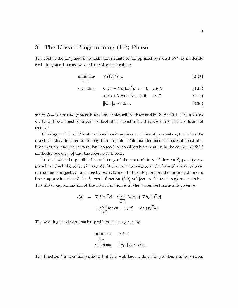
� The Linear Programming �LP� Phase

The goal of the LP phase is to make an estimate of the optimal active set W�� at moderate

cost� In general terms we want to solve the problem

minimizedLP

rfxTdLP ��a

such that hix �rhixT dLP � �� i � E ��b

gix �rgixT dLP � �� i � I ��c

kdLPk� � �LP� ��d

where �LP is a trust�region radius whose choice will be discussed in Section �� The working

set W will be de�ned to be some subset of the constraints that are active at the solution of

this LP�

Working with this LP is attractive since it requires no choice of parameters� but it has the

drawback that its constraints may be infeasible� This possible inconsistency of constraint

linearizations and the trust region has received considerable attention in the context of SQP

methods� see� e�g� �� and the references therein�

To deal with the possible inconsistency of the constraints we follow an ��penalty ap�

proach in which the constraints ��b��c are incorporated in the form of a penalty term

in the model objective� Speci�cally� we reformulate the LP phase as the minimization of a

linear approximation of the �� merit function �� subject to the trust�region constraint�

The linear approximation of the merit function � at the current estimate x is given by

ld � rfxTd� �Xi�E

jhix �rhixT dj

��Xi�I

max��gix�rgixTd�

The working�set determination problem is then given by

minimizedLP

ldLP

such that kdLPk� � �LP�

The function l is non�di�erentiable but it is well�known that this problem can be written

�

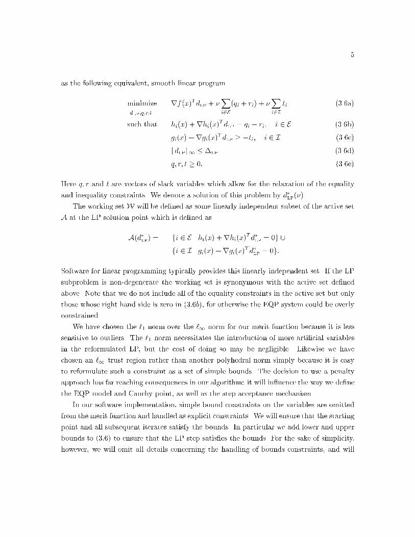
as the following equivalent� smooth linear program

minimizedLP�q�r�t

rfxTdLP � �Xi�E

qi � ri � �Xi�I

ti ��a

such that hix �rhixT dLP � qi � ri� i � E ��b

gix �rgixT dLP � �ti� i � I ��c

kdLPk� � �LP ��d

q� r� t � �� e

Here q� r and t are vectors of slack variables which allow for the relaxation of the equality

and inequality constraints� We denote a solution of this problem by d�LP��

The working set W will be de�ned as some linearly independent subset of the active set

A at the LP solution point which is de�ned as

Ad�LP � fi � E j hix �rhix

T d�LP

� �g �

fi � I j gix �rgixT d�LP � �g�

Software for linear programming typically provides this linearly independent set� If the LP

subproblem is non�degenerate the working set is synonymous with the active set de�ned

above� Note that we do not include all of the equality constraints in the active set but only

those whose right hand side is zero in ��b� for otherwise the EQP system could be overly

constrained�

We have chosen the �� norm over the �� norm for our merit function because it is less

sensitive to outliers� The �� norm necessitates the introduction of more arti�cial variables

in the reformulated LP� but the cost of doing so may be negligible� Likewise we have

chosen an �� trust region rather than another polyhedral norm simply because it is easy

to reformulate such a constraint as a set of simple bounds� The decision to use a penalty

approach has far reaching consequences in our algorithm� it will in�uence the way we de�ne

the EQP model and Cauchy point� as well as the step acceptance mechanism�

In our software implementation� simple bound constraints on the variables are omitted

from the merit function and handled as explicit constraints� We will ensure that the starting

point and all subsequent iterates satisfy the bounds� In particular we add lower and upper

bounds to �� to ensure that the LP step satis�es the bounds� For the sake of simplicity�

however� we will omit all details concerning the handling of bounds constraints� and will

�

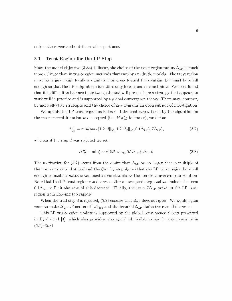
only make remarks about them when pertinent�

�� Trust Region for the LP Step

Since the model objective ��a is linear� the choice of the trust�region radius �LP is much

more delicate than in trust�region methods that employ quadratic models� The trust region

must be large enough to allow signi�cant progress toward the solution� but must be small

enough so that the LP subproblem identi�es only locally active constraints� We have found

that it is di�cult to balance these two goals� and will present here a strategy that appears to

work well in practice and is supported by a global convergence theory� There may� however�

be more e�ective strategies and the choice of �LP remains an open subject of investigation�

We update the LP trust region as follows� If the trial step d taken by the algorithm on

the most current iteration was accepted i�e�� if � � tolerance� we de�ne

��LP

� minmaxf��kdk�� kdCk�� LPg� ��LP� ��

whereas if the step d was rejected we set

��LP � minmaxf��kdk�� LPg��LP� ��

The motivation for �� stems from the desire that �LP be no larger than a multiple of

the norm of the trial step d and the Cauchy step dC� so that the LP trust region be small

enough to exclude extraneous� inactive constraints as the iterate converges to a solution�

Note that the LP trust region can decrease after an accepted step� and we include the term

��LP to limit the rate of this decrease� Finally� the term ��LP prevents the LP trust

region from growing too rapidly�

When the trial step d is rejected� �� ensures that �LP does not grow� We would again

want to make �LP a fraction of kdk�� and the term ��LP limits the rate of decrease�

This LP trust�region update is supported by the global convergence theory presented

in Byrd et al �� which also provides a range of admissible values for the constants in

��

�

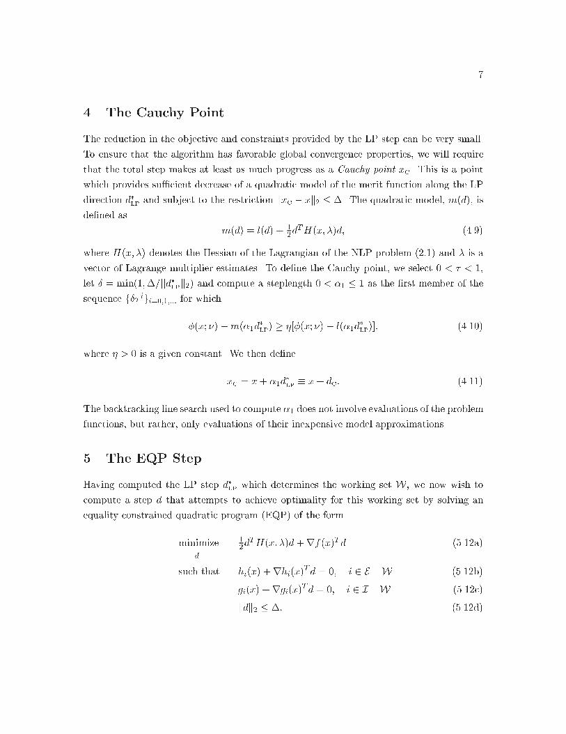
� The Cauchy Point

The reduction in the objective and constraints provided by the LP step can be very small�

To ensure that the algorithm has favorable global convergence properties� we will require

that the total step makes at least as much progress as a Cauchy point xC� This is a point

which provides su�cient decrease of a quadratic model of the merit function along the LP

direction d�LP and subject to the restriction kxC � xk� � �� The quadratic model� md� is

de�ned as

md � ld � ��d

THx� �d� ��

where Hx� � denotes the Hessian of the Lagrangian of the NLP problem �� and � is a

vector of Lagrange multiplier estimates� To de�ne the Cauchy point� we select � ��

let � � min��jjd�LPk� and compute a steplength � �� as the �rst member of the

sequence f� igi�� for which

�x� ��m��d�LP � ��x� � � l��d

�LP��

where � � is a given constant� We then de�ne

xC � x� ��d�LP� x� dC� ��

The backtracking line search used to compute �� does not involve evaluations of the problem

functions� but rather� only evaluations of their inexpensive model approximations�

� The EQP Step

Having computed the LP step d�LP which determines the working set W� we now wish to

compute a step d that attempts to achieve optimality for this working set by solving an

equality constrained quadratic program EQP of the form

minimized

��d

THx� �d �rfxTd ��a

such that hix �rhixT d � �� i � E W ��b

gix �rgixT d � �� i � I W ��c

kdk� � �� d

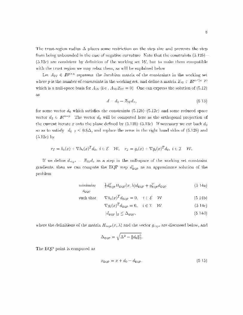
The trust�region radius � places some restriction on the step size and prevents the step

from being unbounded in the case of negative curvature� Note that the constraints ��b�

��c are consistent by de�nition of the working set W� but to make them compatible

with the trust region we may relax them� as will be explained below�

Let AW � IRp�n represent the Jacobian matrix of the constraints in the working set

where p is the number of constraints in the working set� and de�ne a matrix ZW � IRn��n�p�

which is a null�space basis for AW i�e�� AWZW � �� One can express the solution of ��

as

d � d� � ZWdZ� ��

for some vector d� which satis�es the constraints ��b��c and some reduced space

vector dZ � IRn�p� The vector d� will be computed here as the orthogonal projection of

the current iterate x onto the plane de�ned by ��b��c� If necessary we cut back d�

so as to satisfy kd�k� � �� and replace the zeros in the right hand sides of ��b and

��c by

rE � hix �rhixT d�� i � E W� rI � gix �rgix

T d�� i � I W�

If we de�ne dEQP � ZWdZ as a step in the null�space of the working set constraint

gradients� then we can compute the EQP step d�EQP

as an approximate solution of the

problem

minimizedEQP

��d

TEQPHEQPx� �dEQP � gTEQPdEQP ��a

such that rhixTdEQP � �� i � E W ��b

rgixTdEQP � �� i � I W ��c

kdEQPk� � �EQP� ��d

where the de�nitions of the matrix HEQPx� � and the vector gEQP are discussed below� and

�EQP �q�� kd�k

��

The EQP point is computed as

xEQP � x� d� � dEQP� ��

�

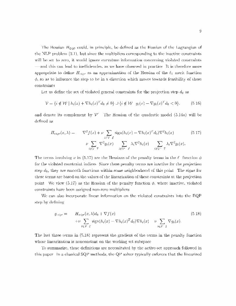
The Hessian HEQP could� in principle� be de�ned as the Hessian of the Lagrangian of

the NLP problem �� but since the multipliers corresponding to the inactive constraints

will be set to zero� it would ignore curvature information concerning violated constraints

� and this can lead to ine�ciencies� as we have observed in practice� It is therefore more

appropriate to de�ne HEQP as an approximation of the Hessian of the �� merit function

�� so as to in�uence the step to be in a direction which moves towards feasibility of these

constraints�

Let us de�ne the set of violated general constraints for the projection step d� as

V � fi �� W j hix �rhixT d� � �g � fi �� W j gix �rgix

T d� �g� ��

and denote its complement by Vc� The Hessian of the quadratic model ��a will be

de�ned as

HEQPx� � � r�fx � �X

i�V�E

signhix �rhixT d�r

�hix ��

��X

i�V�I

r�gix�X

i�Vc�E

�ir�hix�

Xi�Vc�I

�ir�gix�

The terms involving � in �� are the Hessians of the penalty terms in the �� function �

for the violated constraint indices� Since these penalty terms are inactive for the projection

step d�� they are smooth functions within some neighborhood of this point� The signs for

these terms are based on the values of the linearization of these constraints at the projection

point� We view �� as the Hessian of the penalty function �� where inactive� violated

constraints have been assigned non�zero multipliers�

We can also incorporate linear information on the violated constraints into the EQP

step by de�ning

gEQP � HEQPx� �d� �rfx ��

��X

i�V�E

signhix �rhixT d�rhix� �

Xi�V�I

rgix�

The last three terms in �� represent the gradient of the terms in the penalty function

whose linearization is nonconstant on the working set subspace�

To summarize� these de�nitions are necessitated by the active�set approach followed in

this paper� In a classical SQP methods� the QP solver typically enforces that the linearized

��

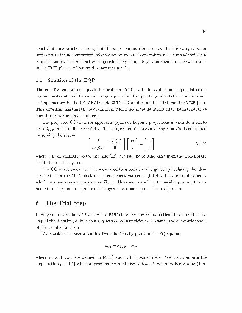
constraints are satis�ed throughout the step computation process� In this case� it is not

necessary to include curvature information on violated constraints since the violated set V

would be empty� By contrast our algorithm may completely ignore some of the constraints

in the EQP phase and we need to account for this�

�� Solution of the EQP

The equality constrained quadratic problem �� with its additional ellipsoidal trust�

region constraint� will be solved using a projected Conjugate�Gradient�Lanczos iteration�

as implemented in the GALAHAD code GLTR of Gould et al �� HSL routine VF��

This algorithm has the feature of continuing for a few more iterations after the �rst negative

curvature direction is encountered�

The projected CG�Lanczos approach applies orthogonal projections at each iteration to

keep dEQP in the null�space of AW � The projection of a vector v� say w � Pv� is computed

by solving the system �I AT

Wx

AWx �

� �w

u

��

�v

�

��

where u is an auxiliary vector� see also �� We use the routine MA�� from the HSL library

�� to factor this system�

The CG iteration can be preconditioned to speed up convergence by replacing the iden�

tity matrix in the �� block of the coe�cient matrix in �� with a preconditioner G

which in some sense approximates HEQP� However� we will not consider preconditioners

here since they require signi�cant changes to various aspects of our algorithm�

� The Trial Step

Having computed the LP� Cauchy and EQP steps� we now combine them to de�ne the trial

step of the iteration� d� in such a way as to obtain su�cient decrease in the quadratic model

of the penalty function�

We consider the vector leading from the Cauchy point to the EQP point�

dCE � xEQP � xC�

where xC and xEQP are de�ned in �� and �� respectively� We then compute the

steplength �� which approximately minimizes m�dCE� where m is given by ��

��

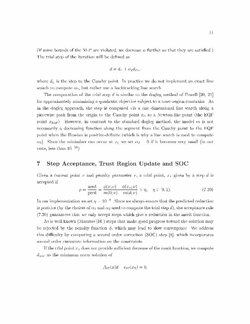
If some bounds of the NLP are violated� we decrease � further so that they are satis�ed�

The trial step of the iteration will be de�ned as

d � dC � ��dCE�

where dC is the step to the Cauchy point� In practice we do not implement an exact line

search to compute �� but rather use a backtracking line search�

The computation of the trial step d is similar to the dogleg method of Powell ��

for approximately minimizing a quadratic objective subject to a trust�region constraint� As

in the dogleg approach� the step is computed via a one dimensional line search along a

piecewise path from the origin to the Cauchy point xC to a Newton�like point the EQP

point xEQP� However� in contrast to the standard dogleg method� the model m is not

necessarily a decreasing function along the segment from the Cauchy point to the EQP

point when the Hessian is positive�de�nite which is why a line search is used to compute

�� Since the minimizer can occur at xC we set �� if it becomes very small in our

tests� less than ��

Step Acceptance Trust Region Update and SOC

Given a current point x and penalty parameter �� a trial point� xT given by a step d is

accepted if

� �ared

pred�

�x� �� xT� �

m�� md� ��

In our implementation we set � �� Since we always ensure that the predicted reduction

is positive by the choices of �� and �� used to compute the trial step d� the acceptance rule

�� guarantees that we only accept steps which give a reduction in the merit function�

As is well known Maratos �� steps that make good progress toward the solution may

be rejected by the penalty function �� which may lead to slow convergence� We address

this di�culty by computing a second order correction SOC step � �� which incorporates

second order curvature information on the constraints�

If the trial point xT does not provide su�cient decrease of the merit function� we compute

dSOC as the minimum norm solution of

AWxd� cWxT � ��

��

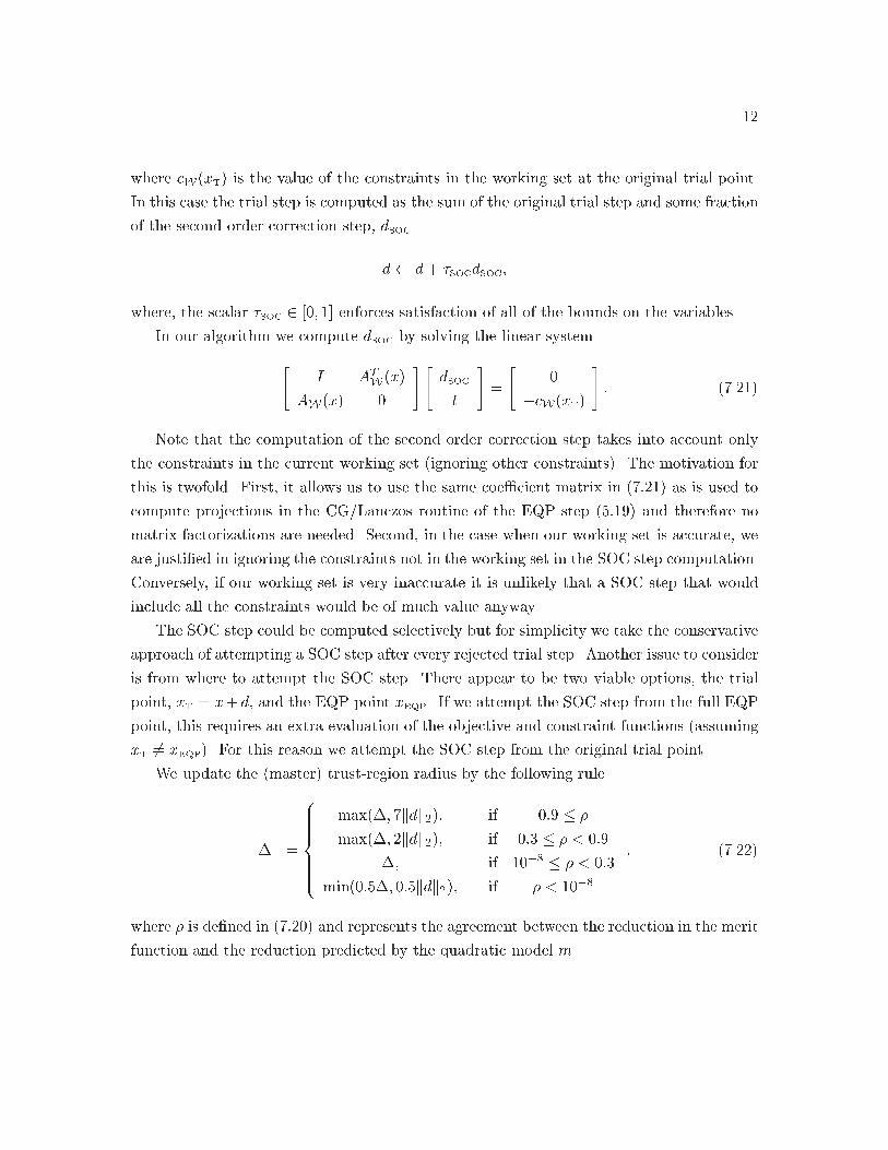
where cWxT is the value of the constraints in the working set at the original trial point�

In this case the trial step is computed as the sum of the original trial step and some fraction

of the second order correction step� dSOC

d� d� SOCdSOC�

where� the scalar SOC � �� enforces satisfaction of all of the bounds on the variables�

In our algorithm we compute dSOC by solving the linear system

�I AT

Wx

AWx �

� �dSOC

t

��

��

�cWxT

��

Note that the computation of the second order correction step takes into account only

the constraints in the current working set ignoring other constraints� The motivation for

this is twofold� First� it allows us to use the same coe�cient matrix in �� as is used to

compute projections in the CG�Lanczos routine of the EQP step �� and therefore no

matrix factorizations are needed� Second� in the case when our working set is accurate� we

are justi�ed in ignoring the constraints not in the working set in the SOC step computation�

Conversely� if our working set is very inaccurate it is unlikely that a SOC step that would

include all the constraints would be of much value anyway�

The SOC step could be computed selectively but for simplicity we take the conservative

approach of attempting a SOC step after every rejected trial step� Another issue to consider

is from where to attempt the SOC step� There appear to be two viable options� the trial

point� xT � x�d� and the EQP point xEQP� If we attempt the SOC step from the full EQP

point� this requires an extra evaluation of the objective and constraint functions assuming

xT � xEQP� For this reason we attempt the SOC step from the original trial point�

We update the master trust�region radius by the following rule

��

��

max�� kdk�� if ��

max�� kdk�� if ��

�� if ��

min�� kdk�� if � ��

� ��

where � is de�ned in �� and represents the agreement between the reduction in the merit

function and the reduction predicted by the quadratic model m�

��

� The Lagrange Multiplier Estimates

Both the LP and the EQP phases of the algorithm provide possible choices for Lagrange

multiplier estimates� However� we choose to compute least�squares Lagrange multipliers

since they satisfy the optimality conditions as well as possible for the given iterate x� and

can be computed very cheaply as we now discuss�

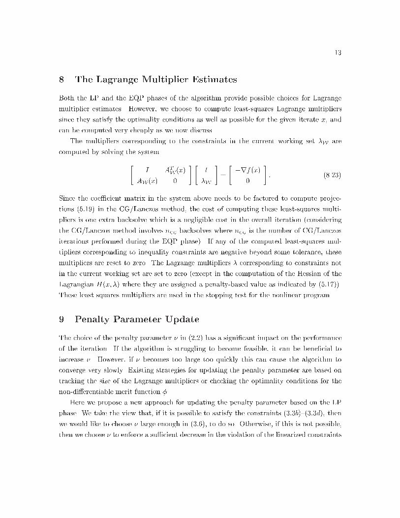
The multipliers corresponding to the constraints in the current working set �W are

computed by solving the system

�I AT

Wx

AWx �

� �t

�W

��

��rfx

�

��

Since the coe�cient matrix in the system above needs to be factored to compute projec�

tions �� in the CG�Lanczos method� the cost of computing these least�squares multi�

pliers is one extra backsolve which is a negligible cost in the overall iteration considering

the CG�Lanczos method involves nCG backsolves where nCG is the number of CG�Lanczos

iterations performed during the EQP phase� If any of the computed least�squares mul�

tipliers corresponding to inequality constraints are negative beyond some tolerance� these

multipliers are reset to zero� The Lagrange multipliers � corresponding to constraints not

in the current working set are set to zero except in the computation of the Hessian of the

Lagrangian Hx� � where they are assigned a penalty�based value as indicated by ��

These least squares multipliers are used in the stopping test for the nonlinear program�

� Penalty Parameter Update

The choice of the penalty parameter � in �� has a signi�cant impact on the performance

of the iteration� If the algorithm is struggling to become feasible� it can be bene�cial to

increase �� However� if � becomes too large too quickly this can cause the algorithm to

converge very slowly� Existing strategies for updating the penalty parameter are based on

tracking the size of the Lagrange multipliers or checking the optimality conditions for the

non�di�erentiable merit function ��

Here we propose a new approach for updating the penalty parameter based on the LP

phase� We take the view that� if it is possible to satisfy the constraints ��b��d� then

we would like to choose � large enough in �� to do so� Otherwise� if this is not possible�

then we choose � to enforce a su�cient decrease in the violation of the linearized constraints

��

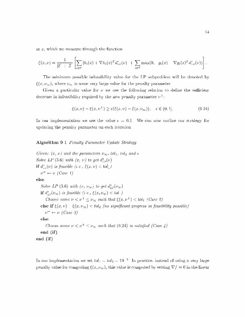
at x� which we measure through the function

�x� � ��

jEj� jIj

�Xi�E

jhix �rhixT d�LP�j �

Xi�I

max��gix�rgixT d�LP�

��

The minimum possible infeasibility value for the LP subproblem will be denoted by

�x� �� where �� is some very large value for the penalty parameter�

Given a particular value for � we use the following relation to de�ne the su�cient

decrease in infeasibility required by the new penalty parameter ��

�x� �� x� �� x� �� x� ��

In our implementation we use the value � � �� We can now outline our strategy for

updating the penalty parameter on each iteration�

Algorithm �� Penalty Parameter Update Strategy

Given� �x� �� and the parameters �� tol�� tol� and ��

Solve LP �� with �x� �� to get d�LP��

if d�LP� is feasible �i�e�� x� � tol��

�� Case ��

else

Solve LP �� with �x� �� to get d�LP��

if d�LP�� is feasible �i�e�� x� �� tol��

Choose some � �� such that �x� �� tol� �Case ��

else if �x� �� x� �� tol� �no signi�cant progress in feasibility possible�

�� Case ��

else

Choose some � �� such that �� is satis�ed �Case ��

end �if�

end �if�

In our implementation we set tol� � tol� � �� In practice� instead of using a very large

penalty value for computing �x� �� this value is computed by setting rf � � in the linear

��

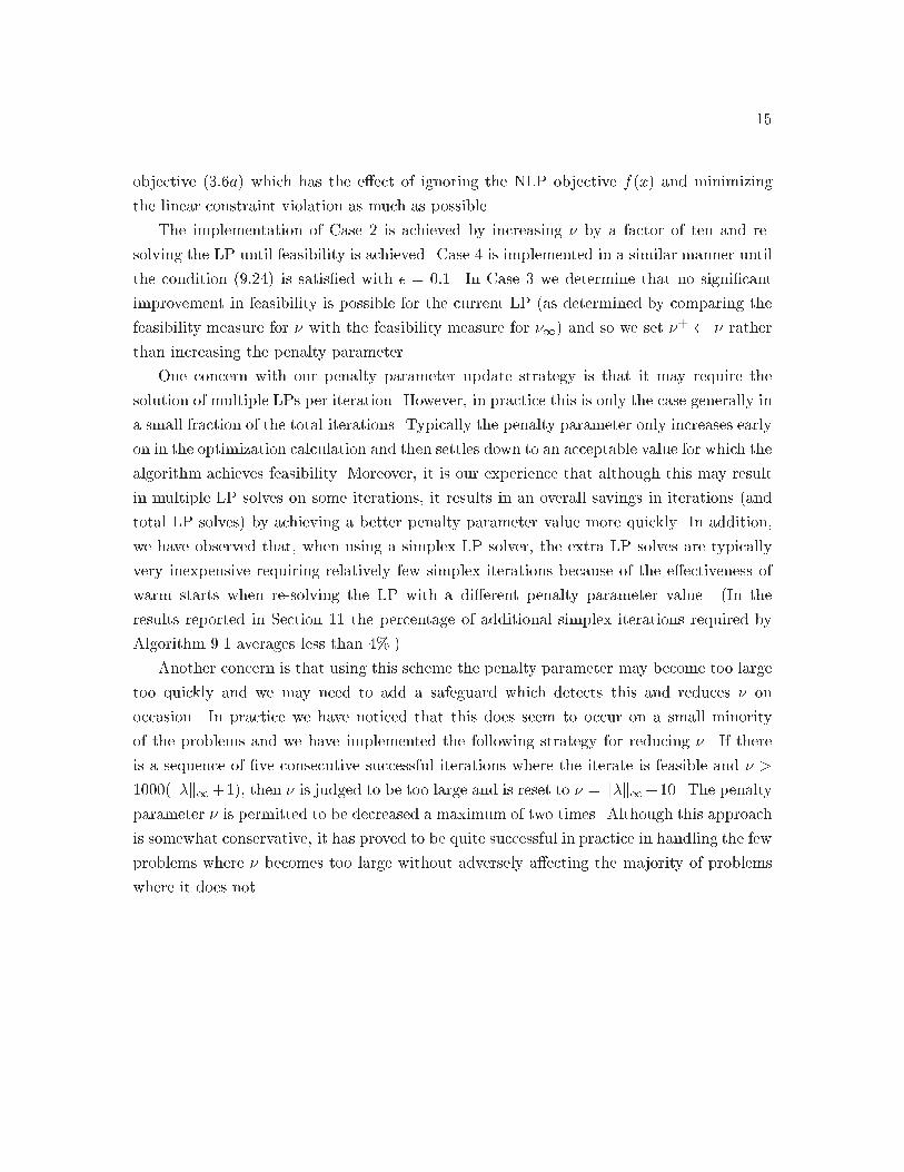
objective ��a which has the e�ect of ignoring the NLP objective fx and minimizing

the linear constraint violation as much as possible�

The implementation of Case � is achieved by increasing � by a factor of ten and re�

solving the LP until feasibility is achieved� Case � is implemented in a similar manner until

the condition �� is satis�ed with � � �� In Case � we determine that no signi�cant

improvement in feasibility is possible for the current LP as determined by comparing the

feasibility measure for � with the feasibility measure for �� and so we set �� rather

than increasing the penalty parameter�

One concern with our penalty parameter update strategy is that it may require the

solution of multiple LPs per iteration� However� in practice this is only the case generally in

a small fraction of the total iterations� Typically the penalty parameter only increases early

on in the optimization calculation and then settles down to an acceptable value for which the

algorithm achieves feasibility� Moreover� it is our experience that although this may result

in multiple LP solves on some iterations� it results in an overall savings in iterations and

total LP solves by achieving a better penalty parameter value more quickly� In addition�

we have observed that� when using a simplex LP solver� the extra LP solves are typically

very inexpensive requiring relatively few simplex iterations because of the e�ectiveness of

warm starts when re�solving the LP with a di�erent penalty parameter value� In the

results reported in Section �� the percentage of additional simplex iterations required by

Algorithm �� averages less than �!�

Another concern is that using this scheme the penalty parameter may become too large

too quickly and we may need to add a safeguard which detects this and reduces � on

occasion� In practice we have noticed that this does seem to occur on a small minority

of the problems and we have implemented the following strategy for reducing �� If there

is a sequence of �ve consecutive successful iterations where the iterate is feasible and � �

��k�k�� then � is judged to be too large and is reset to � � k�k�� The penalty

parameter � is permitted to be decreased a maximum of two times� Although this approach

is somewhat conservative� it has proved to be quite successful in practice in handling the few

problems where � becomes too large without adversely a�ecting the majority of problems

where it does not�

��

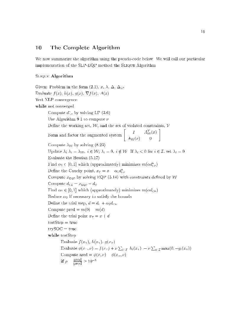
� The Complete Algorithm

We now summarize the algorithm using the pseudo�code below� We will call our particular

implementation of the SLP�EQP method the Slique Algorithm�

Slique Algorithm

Given� Problem in the form �� x� �� LP�

Evaluate fx� hx� gx� rfx� Ax�

Test NLP convergence�

while not converged

Compute d�LP by solving LP ��

Use Algorithm �� to compute ��

De�ne the working set� W� and the set of violated constraints� V�

Form and factor the augmented system

�I AT

Wx

AWx �

��

Compute �W by solving ��

Update �� i � �W � i � W� �i � �� i �� W� If �i � for i � I� set �i � ��

Evaluate the Hessian ��

Find �� which approximately minimizes m�d�LP�

De�ne the Cauchy point� xC � x� ��d�LP�

Compute xEQP by solving EQP �� with constraints de�ned by W�

Compute dCE � xEQP � dC�

Find �� which approximately minimizes m�dCE�

Reduce �� if necessary to satisfy the bounds�

De�ne the trial step� d � dC � ��dCE�

Compute pred � m��md�

De�ne the trial point xT � x� d�

testStep � true�

trySOC � true�

while testStep

Evaluate fxT� hxT� gxT�

Evaluate �xT� � � fxT � �P

i�E jhixTj� �P

i�I max��gixT�

Compute ared � �x� �� xT� ��

if � � aredpred � ��

��

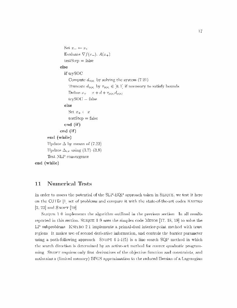
Set x� � xT�

Evaluate rfx�� Ax��

testStep � false�

else

if trySOC

Compute dSOC by solving the system ��

Truncate dSOC by SOC � �� if necessary to satisfy bounds�

De�ne xT � x� d� SOCdSOC�

trySOC � false�

else

Set x� � x�

testStep � false�

end �if�

end �if�

end �while�

Update � by means of ��

Update �LP using ��

Test NLP convergence�

end �while�

�� Numerical Tests

In order to assess the potential of the SLP�EQP approach taken in Slique� we test it here

on the CUTEr �� set of problems and compare it with the state�of�the�art codes Knitro

�� and Snopt ��

Slique �� implements the algorithm outlined in the previous section� In all results

reported in this section� Slique �� uses the simplex code Minos �� to solve the

LP subproblems� Knitro �� implements a primal�dual interior�point method with trust

regions� It makes use of second derivative information� and controls the barrier parameter

using a path�following approach� Snopt �� is a line search SQP method in which

the search direction is determined by an active�set method for convex quadratic program�

ming� Snopt requires only �rst derivatives of the objective function and constraints� and

maintains a limited memory BFGS approximation to the reduced Hessian of a Lagrangian

�

function� Even though Snopt uses only �rst derivatives whereas Knitro and Slique use

second derivatives it provides a worthy benchmark for our purposes since it is generally

regarded as one of the most e�ective active�set SQP codes available for large�scale nonlinear

optimization�

All tests described in this paper were performed on a Sun Ultra �� with �Gb of memory

running SunOS �� All codes are written in FORTRAN� were compiled using the Sun f��

compiler with the �O� compilation �ag� and were run in double precision using all their

default settings� For Snopt� the superbasics limit was increased to �� to allow for the

solution of the majority of the CUTEr problems� However� for some problems this limit was

still too small and so for these problems the superbasics limit was increased even more until

it was su�ciently large� Limits of � hour of CPU time and �� outer or major iterations

were imposed for each problem� if one of these limits was reached the code was considered

to have failed� The stopping tolerance was set at �� for all solvers� Although� it is nearly

impossible to enforce a uniform stopping condition� the stopping conditions for Slique and

Knitro were constructed to be very similar to that used in Snopt�

�� Robustness

In order to �rst get a picture of the robustness of the Slique algorithm we summarize

its performance on a subset of problems from the CUTEr test set as of May ��

Since we are primarily interested in the performance of Slique on general nonlinear opti�

mization problems with inequality constraints and�or bounds on the variables such that

the active�set identi�cation mechanism is relevant� we exclude all unconstrained prob�

lems and problems whose only constraints are equations or �xed variables� We also ex�

clude LPs and feasibility problems problems with zero degrees of freedom� In addi�

tion eight problems ALLINQP� CHARDIS�� CHARDIS�� CONT��QQ� DEGENQP� HARKERP��

LUBRIF� ODNAMUR were removed because they could not be comfortably run within the

memory limits of the testing machine for any of the codes� The remaining �� problems

form our test set� These remaining problems can be divided between three sets� quadratic

programs QP� problems whose only constraints are simple bounds on the variables BC�

and everything else� which we refer to as generally constrained GC problems� If a problem

is a QP just involving bound constraints� it is included only in the BC set�

Although we will not show it here� the SLP�EQP algorithm described in this paper is

quite robust and e�cient at solving simpler classes of problems e�g�� LPs� unconstrained

��

problems� equality constrained problems and feasibility problems as evidenced in ��

We should note that there are a few problems in CUTEr for which a solution does not

exist for example the problem may be infeasible or unbounded� Although� it is important

for a code to recognize and behave intelligently in these cases� we do not evaluate the ability

of a code to do so here� For simplicity� we treat all instances where an optimal solution is

not found as a failure regardless of whether or not it is possible to �nd such a point�

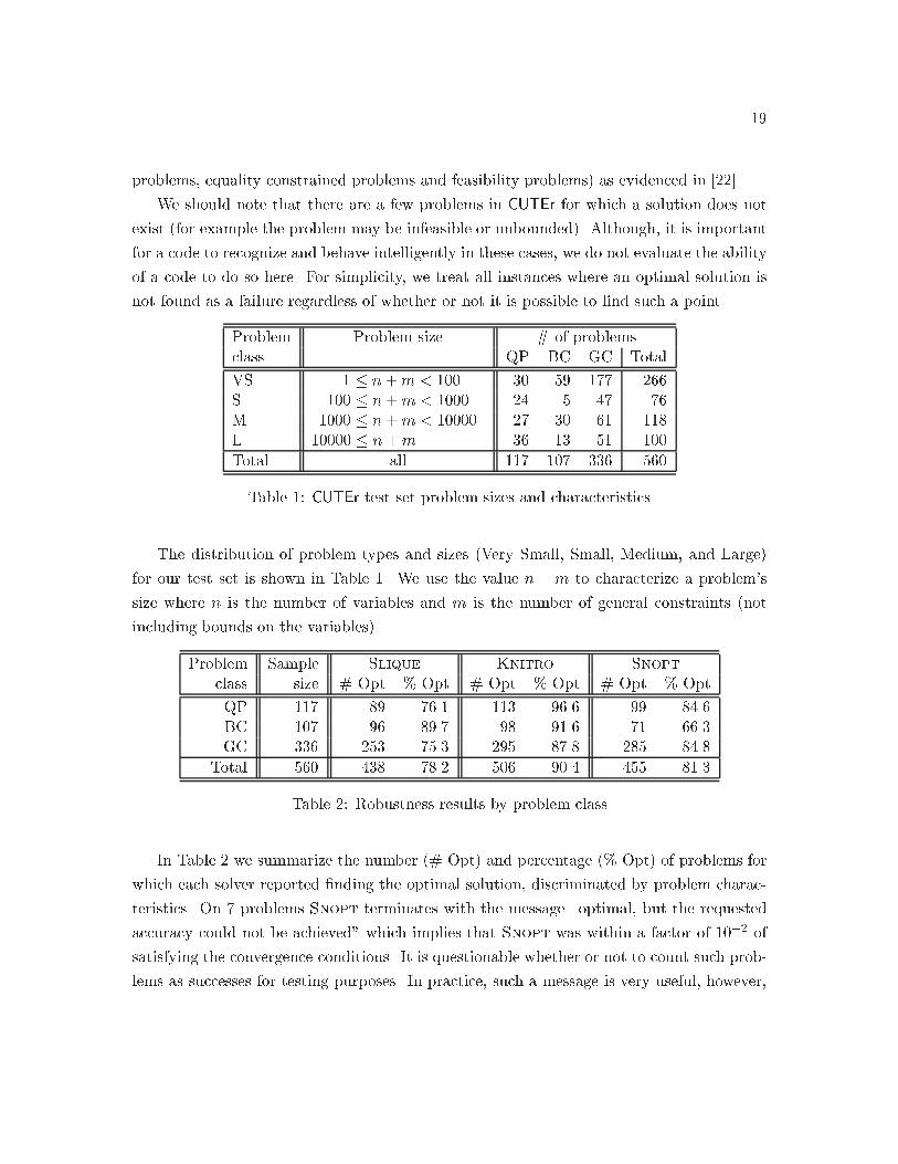
Problem Problem size " of problemsclass QP BC GC Total

VS � � n�m �� S �� n�m �� M �� n�m �� L �� n�m ��

Total all ��

Table �� CUTEr test set problem sizes and characteristics

The distribution of problem types and sizes Very Small� Small� Medium� and Large

for our test set is shown in Table �� We use the value n �m to characterize a problem#s

size where n is the number of variables and m is the number of general constraints not

including bounds on the variables�

Problem Sample Slique Knitro Snopt

class size " Opt ! Opt " Opt ! Opt " Opt ! Opt

QP �� BC �� GC ��

Total ��

Table �� Robustness results by problem class

In Table � we summarize the number " Opt and percentage ! Opt of problems for

which each solver reported �nding the optimal solution� discriminated by problem charac�

teristics� On � problems Snopt terminates with the message optimal� but the requested

accuracy could not be achieved� which implies that Snopt was within a factor of �� of

satisfying the convergence conditions� It is questionable whether or not to count such prob�

lems as successes for testing purposes� In practice� such a message is very useful� however�

��

both Slique andKnitro report any problem for which it cannot meet the desired accuracy

in the stopping condition as a failure� even if it comes very close and it is suspected that

the iterate has converged to a locally optimal point� Therefore� in order to be consistent�

we do not count these problems as successes for Snopt� Since the number of such problems

is small relatively speaking� their overall e�ect is negligible�

Even though Slique is signi�cantly less robust than the solver Knitro it is nearly as

robust� overall� as Snopt� We �nd this encouraging since many features of our software

implementation can be improved� as discussed in the �nal section of this paper�

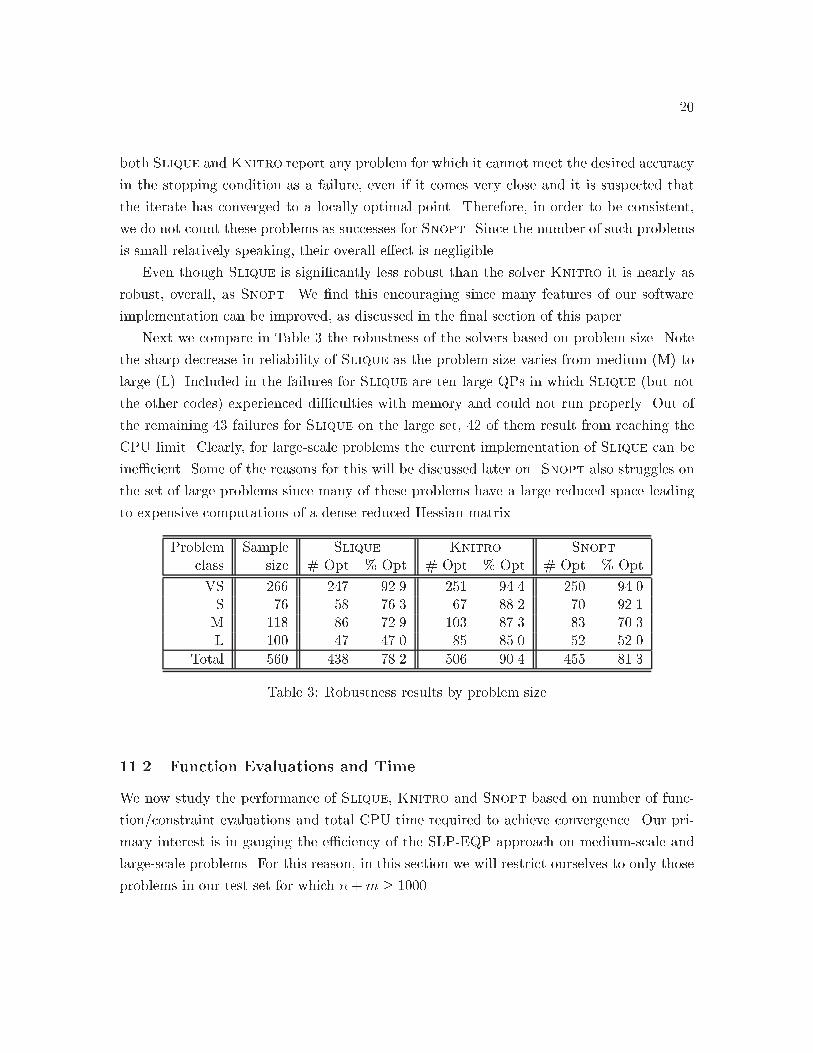
Next we compare in Table � the robustness of the solvers based on problem size� Note

the sharp decrease in reliability of Slique as the problem size varies from medium M to

large L� Included in the failures for Slique are ten large QPs in which Slique but not

the other codes experienced di�culties with memory and could not run properly� Out of

the remaining �� failures for Slique on the large set� �� of them result from reaching the

CPU limit� Clearly� for large�scale problems the current implementation of Slique can be

ine�cient� Some of the reasons for this will be discussed later on� Snopt also struggles on

the set of large problems since many of these problems have a large reduced space leading

to expensive computations of a dense reduced Hessian matrix�

Problem Sample Slique Knitro Snopt

class size " Opt ! Opt " Opt ! Opt " Opt ! Opt

VS �� S �� M �� L ��

Total ��

Table �� Robustness results by problem size

�� Function Evaluations and Time

We now study the performance of Slique� Knitro and Snopt based on number of func�

tion�constraint evaluations and total CPU time required to achieve convergence� Our pri�

mary interest is in gauging the e�ciency of the SLP�EQP approach on medium�scale and

large�scale problems� For this reason� in this section we will restrict ourselves to only those

problems in our test set for which n�m � ��

��

For the number of function�constraint evaluations we take the maximum of these two

quantities� In order to ensure that the timing results are as accurate as possible� all tests

involving timing were carried out on a dedicated machine with no other jobs running�

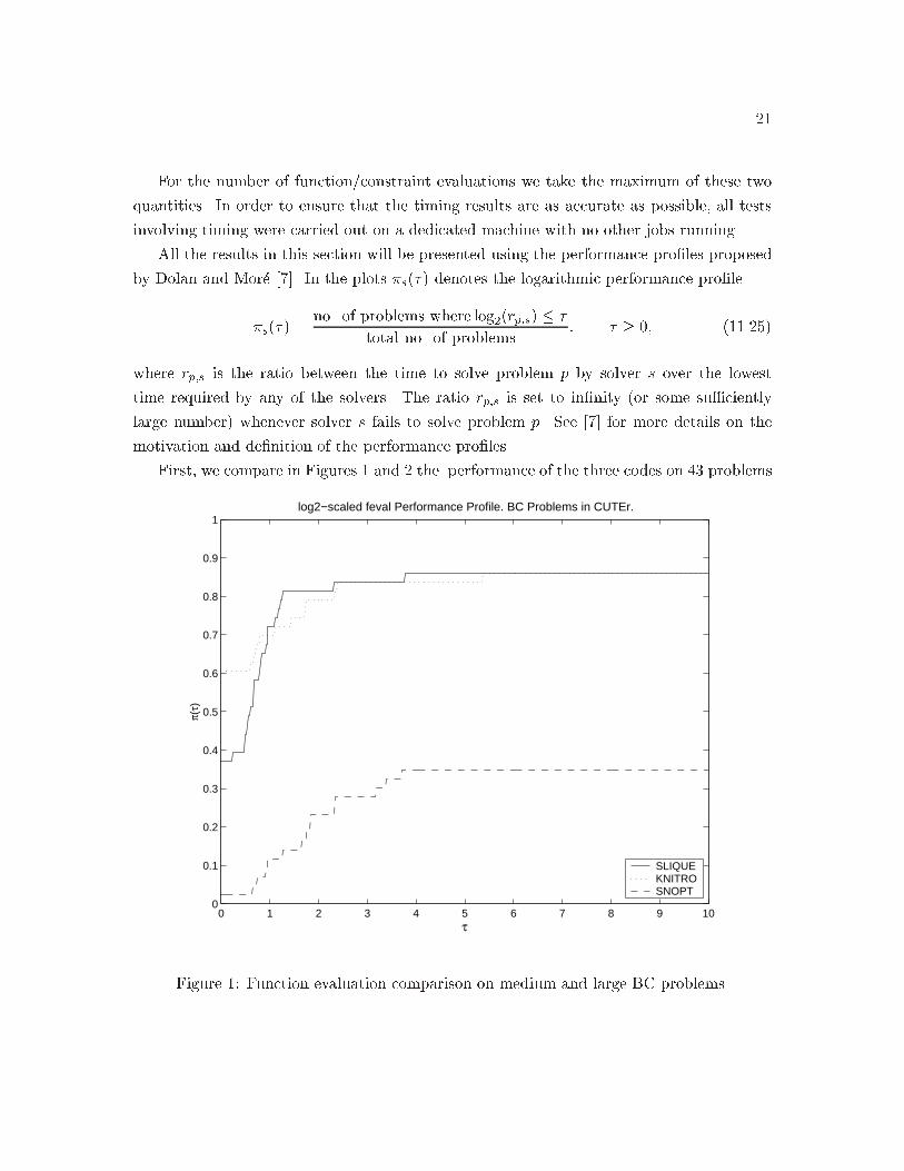
All the results in this section will be presented using the performance pro�les proposed

by Dolan and Mor$e �� In the plots �s denotes the logarithmic performance pro�le

�s �no� of problems where log�rp�s �

total no� of problems� � ��

where rp�s is the ratio between the time to solve problem p by solver s over the lowest

time required by any of the solvers� The ratio rp�s is set to in�nity or some su�ciently

large number whenever solver s fails to solve problem p� See �� for more details on the

motivation and de�nition of the performance pro�les�

First� we compare in Figures � and � the performance of the three codes on �� problems

0 1 2 3 4 5 6 7 8 9 100

0.1

0.2

0.3

0.4

0.5

0.6

0.7

0.8

0.9

1

τ

π(τ)

log2−scaled feval Performance Profile. BC Problems in CUTEr.

SLIQUEKNITROSNOPT

Figure �� Function evaluation comparison on medium and large BC problems�

��

0 1 2 3 4 5 6 7 8 9 100

0.1

0.2

0.3

0.4

0.5

0.6

0.7

0.8

0.9

1

τ

π(τ)

log2−scaled CPU Performance Profile. BC Problems in CUTEr.

SLIQUEKNITROSNOPT

Figure �� CPU comparison on medium and large BC problems�

whose only constraints are simple bounds on the variables� Although there exist specialized

approaches for solving these types of problems �� it is instructive to observe the

performance of Slique when the feasible region has the simple geometry produced by simple

bounds� Figures � and � indicate that Slique performs quite well on this class of problems�

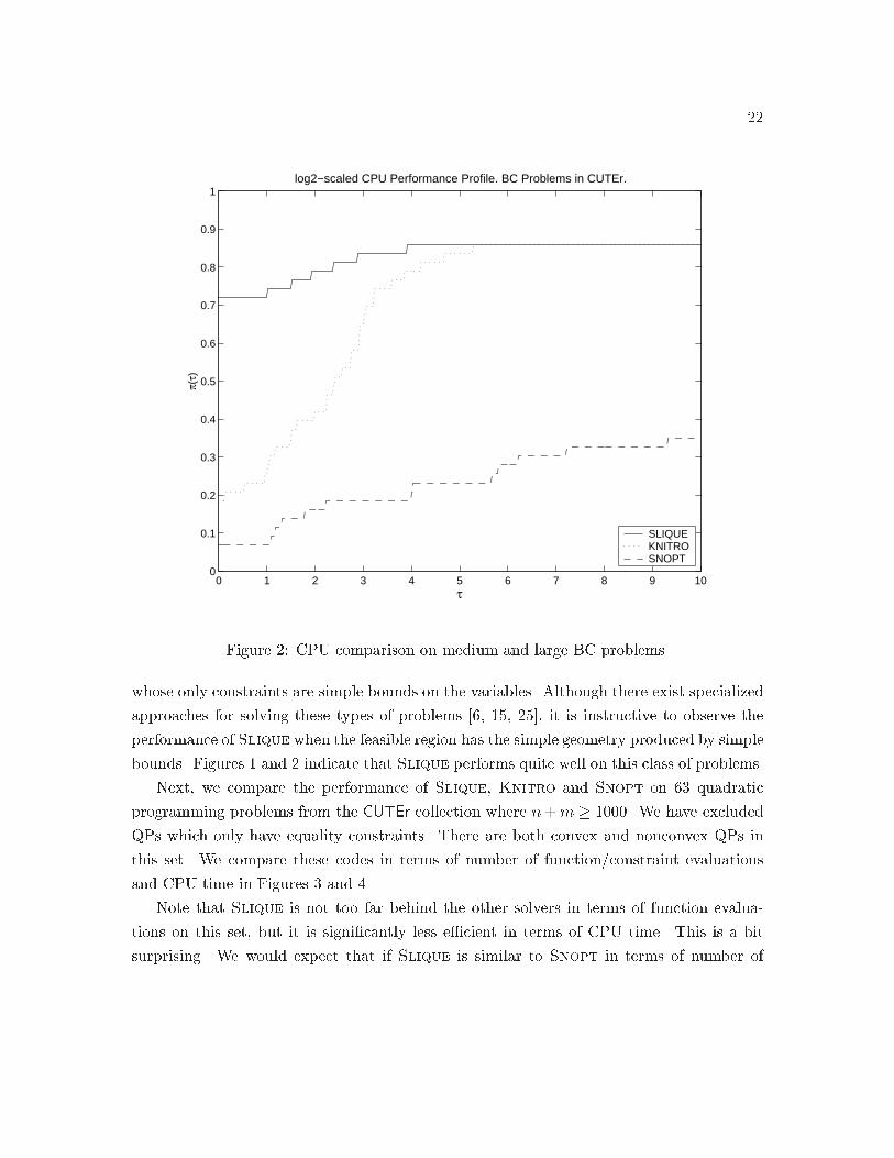
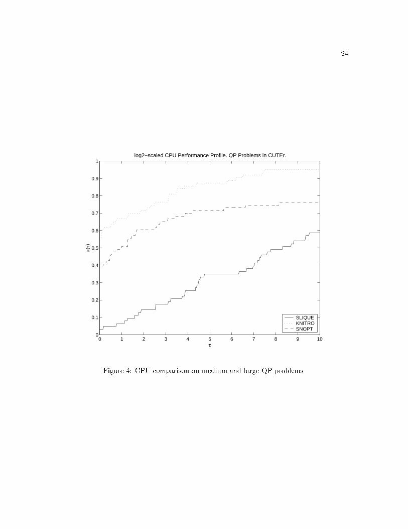
Next� we compare the performance of Slique� Knitro and Snopt on �� quadratic

programming problems from the CUTEr collection where n�m � �� We have excluded

QPs which only have equality constraints� There are both convex and nonconvex QPs in

this set� We compare these codes in terms of number of function�constraint evaluations

and CPU time in Figures � and ��

Note that Slique is not too far behind the other solvers in terms of function evalua�

tions on this set� but it is signi�cantly less e�cient in terms of CPU time� This is a bit

surprising� We would expect that if Slique is similar to Snopt in terms of number of

��

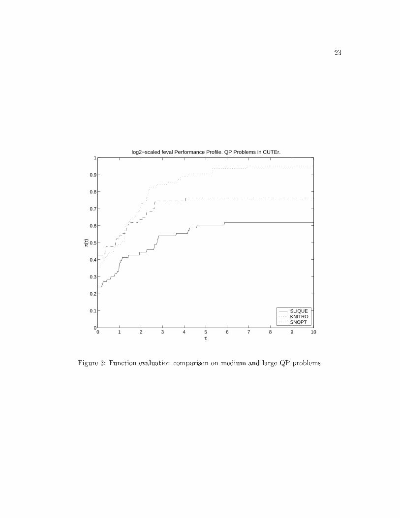
0 1 2 3 4 5 6 7 8 9 100

0.1

0.2

0.3

0.4

0.5

0.6

0.7

0.8

0.9

1

τ

π(τ)

log2−scaled feval Performance Profile. QP Problems in CUTEr.

SLIQUEKNITROSNOPT

Figure �� Function evaluation comparison on medium and large QP problems�

��

0 1 2 3 4 5 6 7 8 9 100

0.1

0.2

0.3

0.4

0.5

0.6

0.7

0.8

0.9

1

τ

π(τ)

log2−scaled CPU Performance Profile. QP Problems in CUTEr.

SLIQUEKNITROSNOPT

Figure �� CPU comparison on medium and large QP problems�

��

function evaluations� that it would also be comparable or perhaps more e�cient in terms

of time� since in general we expect an SLP�EQP iteration to be cheaper than an active�set

SQP iteration and typically the number of function evaluations is similar to the number

of iterations� In many of these cases� the average number of inner simplex iterations of

the LP solver per outer iteration in Slique greatly exceeds the average number of inner

QP iterations per outer iteration in Snopt� This is caused� in part� by the inability of the

current implementation of Slique to perform e�ective warm starts� as will be discussed in

Section ��

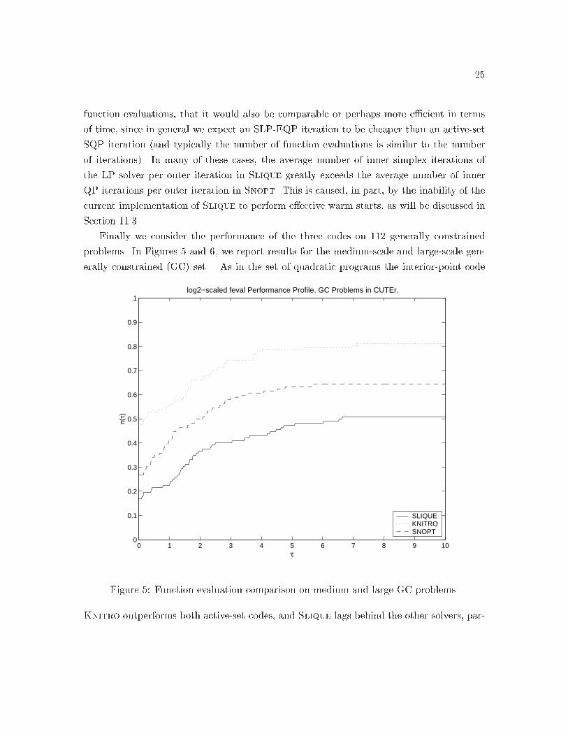
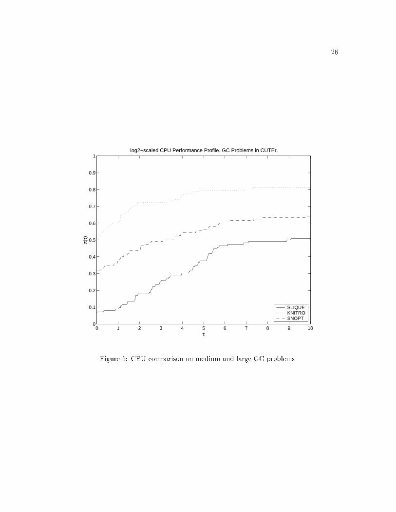
Finally we consider the performance of the three codes on �� generally constrained

problems� In Figures � and �� we report results for the medium�scale and large�scale gen�

erally constrained GC set� As in the set of quadratic programs the interior�point code

0 1 2 3 4 5 6 7 8 9 100

0.1

0.2

0.3

0.4

0.5

0.6

0.7

0.8

0.9

1

τ

π(τ)

log2−scaled feval Performance Profile. GC Problems in CUTEr.

SLIQUEKNITROSNOPT

Figure �� Function evaluation comparison on medium and large GC problems�

Knitro outperforms both active�set codes� and Slique lags behind the other solvers� par�

��

0 1 2 3 4 5 6 7 8 9 100

0.1

0.2

0.3

0.4

0.5

0.6

0.7

0.8

0.9

1

τ

π(τ)

log2−scaled CPU Performance Profile. GC Problems in CUTEr.

SLIQUEKNITROSNOPT

Figure �� CPU comparison on medium and large GC problems�

��

ticularly in terms of CPU time�

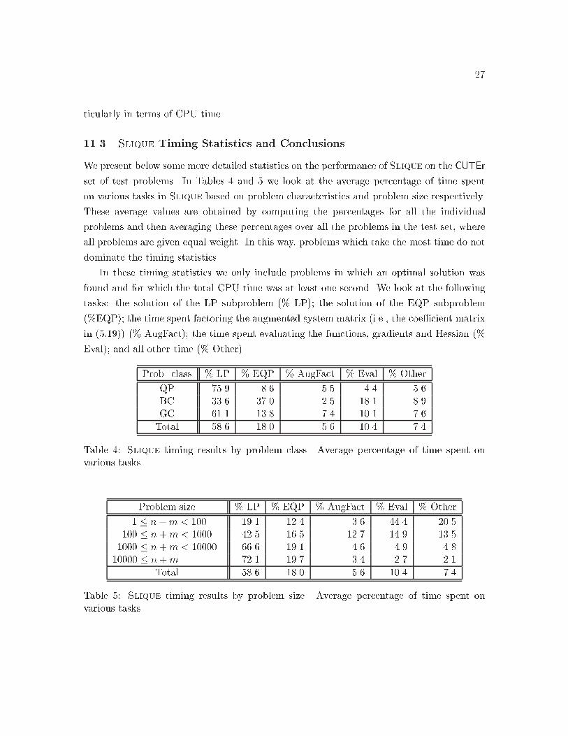
�� Slique Timing Statistics and Conclusions

We present below some more detailed statistics on the performance of Slique on the CUTEr

set of test problems� In Tables � and � we look at the average percentage of time spent

on various tasks in Slique based on problem characteristics and problem size respectively�

These average values are obtained by computing the percentages for all the individual

problems and then averaging these percentages over all the problems in the test set� where

all problems are given equal weight� In this way� problems which take the most time do not

dominate the timing statistics�

In these timing statistics we only include problems in which an optimal solution was

found and for which the total CPU time was at least one second� We look at the following

tasks� the solution of the LP subproblem ! LP� the solution of the EQP subproblem

!EQP� the time spent factoring the augmented system matrix i�e�� the coe�cient matrix

in �� ! AugFact� the time spent evaluating the functions� gradients and Hessian !

Eval� and all other time ! Other�

Prob� class ! LP ! EQP ! AugFact ! Eval ! Other

QP �� BC �� GC ��

Total � ��

Table �� Slique timing results by problem class� Average percentage of time spent onvarious tasks�

Problem size ! LP ! EQP ! AugFact ! Eval ! Other

� � n�m �� n�m �� n�m �� n�m ��

Total � ��

Table �� Slique timing results by problem size� Average percentage of time spent onvarious tasks�

�

It is apparent from these tables that� in general� the solution of the LP subproblems

dominates the overall cost of the algorithm with the solution of the EQP being the second

most costly feature� An exception is the class of bound constrained problems where the

computational work is shared roughly equally between the LP and EQP phases� For the

other problem classes� it is surprising the degree to which the LP solves dominate the overall

time as the size of the problem grows�

Upon further examination� it is clear that there are two sources for the excessive LP

times� For some problems� the �rst few iterations of Slique require a very large number of

simplex steps� On other problems� the number of LP iterations does not decrease substan�

tially as the solution of the nonlinear program is approached� i�e�� the warm start feature

is not completely successful� Designing an e�ective warm start technique for our SLP�EQP

approach is a challenging research question� since the set of constraints active at the solu�

tion of the LP subproblem often include many trust�region constraints which may change

from one iteration to the next even when the optimal active set for the NLP is identi�ed�

In contrast� warm starts are generally e�ective in Snopt for which the number of inner

iterations decreases rapidly near the solution�

We conclude this section by making the following summary observations about the

algorithm� based on the tests reported here� see also ��

� Slique is currently quite robust and e�cient for small and medium�size problems� It

is very e�ective for bound constrained problems of all sizes� where the LP and EQP

costs are well balanced�

� The strategy for updating the penalty parameter � in Slique has proved to be ef�

fective� Typically it chooses an adequate value of � quickly and keeps it constant

thereafter in our tests� �! of the iterations used the �nal value of �� and � was

increased less than once per problem on the average� Therefore� the choice of the

penalty parameter does not appear to be a problematic issue in our approach�

� The active set identi�cation properties of the LP phase are� generally� e�ective� This

is one of the most positive observations of this work� Nevertheless� in some problems

Slique has di�culties identifying the active set near the solution� which indicates

that more work is needed to improve our LP trust region update mechanism�

� The active�set codes� Slique and Snopt are both signi�cantly less robust and e�cient

for large�scale problems overall� compared to the interior�point code Knitro� It

��

appears that these codes perform poorly on large problems for di�erent reasons� The

SQP approach implemented by Snopt is ine�cient on large�scale problems because

many of these have a large reduced space leading to high computing times for the QP

subproblems� However� a large reduced space is not generally a di�culty for Slique

as evidenced by its performance on the bound constrained problems�

By contrast� the SLP�EQP approach implemented in Slique becomes ine�cient for

large�scale problems because of the large computing times in solving the LP problem�

It is not known to us whether these ine�ciencies can be overcome simply by using a

more powerful�perhaps interior�point based�linear programming solver� or if they

require more substantial changes to the algorithm� Warm starts in Snopt� however�

appear to be very e�cient�

�� Final Remarks

We have presented a new active�set� trust�region algorithm for large�scale optimization� It

is based on the SLP�EQP approach of Fletcher and Sainz de la Maza� Among the novel

features of our algorithm we can mention� i a new procedure for computing the EQP step

using a quadratic model of the penalty function and a trust region� ii a dogleg approach for

computing the total step based on the Cauchy and EQP steps� iii an automatic procedure

for adjusting the penalty parameter using the linear programming subproblem� iv a new

procedure for updating the LP trust�region radius that allows it to decrease even on accepted

steps to promote the identi�cation of locally active constraints�

The experimental results presented in Section �� indicate� in our opinion� that the algo�

rithm holds much promise� In addition� the algorithm is supported by the global convergence

theory presented in �� which builds upon the analysis of Yuan ��

Our approach di�ers signi�cantly from the SLP�EQP algorithm described by Fletcher

and Chin �� These authors use a �lter for step acceptance� In the event that the con�

straints in the LP subproblem are incompatible� their algorithm solves instead a feasibility

problem that minimizes the violation of the constraints while ignoring the objective func�

tion� We prefer the ��penalty approach �� because it allows us to work simultaneously

on optimality and feasibility� but testing would be needed to establish which approach is

preferable� The algorithm of Fletcher and Chin de�nes the trial step to be either the full

step to the EQP point plus possibly a second order correction or if this step is unaccept�

able the Cauchy step� In contrast� our approach explores a dogleg path to determine the

��

full step� Our algorithm also di�ers in the way the LP trust region is handled and many

other algorithmic aspects�

The software used to implement the Slique algorithm is not a �nished product but rep�

resents the �rst stage in algorithmic development� In our view� it is likely that signi�cant

improvements in the algorithm can be made by developing� i faster procedures for solving

the LP subproblem� including better initial estimates of the active set� ii improved strate�

gies for updating the LP trust region� iii an improved second�order correction strategy or

a replacement by a non�monotone strategy� iv preconditioning techniques for solving the

EQP step� v mechanisms for handling degeneracy�

��

References

�� I� Bongartz� A� R� Conn� N� I� M� Gould� and Ph� L� Toint� CUTE� Constrained andUnconstrained Testing Environment� ACM Transactions on Mathematical Software��

�� R� H� Byrd� M� E� Hribar� and J� Nocedal� An interior point algorithm for large scalenonlinear programming� SIAM Journal on Optimization� ��

�� R�H� Byrd� N�I�M� Gould� J� Nocedal� and R�A� Waltz� On the convergence of analgorithm for composite nonsmooth optimization� Technical Report OTC �� Op�timization Technology Center� Northwestern University� Evanston� IL� USA� ��

�� C� M� Chin and R� Fletcher� On the global convergence of an SLP��lter algorithm thattakes EQP steps� Numerical Analysis Report NA�� Department of Mathematics�University of Dundee� Dundee� Scotland� ��

�� A� R� Conn� N� I� M� Gould� and Ph� Toint� Trust�region methods� MPS�SIAM Serieson Optimization� SIAM publications� Philadelphia� PA� USA� ��

�� A� R� Conn� N� I� M� Gould� and Ph� L� Toint� LANCELOT� a Fortran package for

Large�scale Nonlinear Optimization �Release A�� Springer Series in ComputationalMathematics� Springer Verlag� Heidelberg� Berlin� New York� ��

�� E� D� Dolan and J� J� Mor$e� Benchmarking optimization software with performancepro�les� Mathematical Programming� Series A� ��

� � R� Fletcher� Practical Methods of Optimization� Volume �� Constrained Optimization�J� Wiley and Sons� Chichester� England� ��

�� R� Fletcher and E� Sainz de la Maza� Nonlinear programming and nonsmooth optimiza�tion by successive linear programming� Mathematical Programming� ��

�� P� E� Gill� W� Murray� and M� A� Saunders� SNOPT� An SQP algorithm for large�scaleconstrained optimization� SIAM Journal on Optimization� ��

�� P� E� Gill� W� Murray� and M� H� Wright� Practical Optimization� Academic Press�London� ��

�� N� I� M� Gould� M� E� Hribar� and J� Nocedal� On the solution of equality constrainedquadratic problems arising in optimization� SIAM Journal on Scienti�c Computing��

��

�� N� I� M� Gould� S� Lucidi� M� Roma� and Ph� L� Toint� Solving the trust�regionsubproblem using the Lanczos method� SIAM Journal on Optimization� ��

�� Harwell Subroutine Library� A catalogue of subroutines �HSL �� AEA Technology�Harwell� Oxfordshire� England� ��

�� C� Lin and J� J� Mor$e� Newton#s method for large bound�constrained optimizationproblems� SIAM Journal on Optimization� ��

�� N� Maratos� Exact penalty function algorithms for �nite�dimensional and control opti�

mization problems� PhD thesis� University of London� London� England� ��

�� B� A� Murtagh and M� A� Saunders� Large�scale linearly constrained optimization�Mathematical Programming� ��

�� B� A� Murtagh and M� A� Saunders� A projected lagrangian algorithm and its imple�mentation for sparse nonlinear constraints� Math� Prog� Study� ��

�� B� A� Murtagh and M� A� Saunders� MINOS �� user#s guide� Technical report� SOL ��R� Systems Optimization Laboratory� Stanford University� �� Revised ��

�� M� J� D� Powell� A Fortran subroutine for unconstrained minimization requiring �rstderivatives of the objective function� Technical Report R�� AERE Harwell Labo�ratory� Harwell� Oxfordshire� England� ��

�� M� J� D� Powell� A new algorithm for unconstrained optimization� In J� B� Rosen� O� L�Mangasarian� and K� Ritter� editors� Nonlinear Programming� pages �� London�� Academic Press�

�� R� A� Waltz� Algorithms for large�scale nonlinear optimization� PhD thesis� Departmentof Electrical and Computer Engineering� Northwestern University� Evanston� Illinois�USA� http��www�ece�northwestern�edu�%rwaltz��

�� R� A� Waltz and J� Nocedal� KNITRO �� user#s manual� Technical Report OTC�� Optimization Technology Center� Northwestern University� Evanston� IL�USA� January ��

�� Y� Yuan� Conditions for convergence of trust region algorithms for nonsmooth opti�mization� Mathematical Programming� ��

�� C� Zhu� R� H� Byrd� P� Lu� and J� Nocedal� Algorithm � � L�BFGS�B� Fortran sub�routines for large�scale bound constrained optimization� ACM Transactions on Math�

ematical Software� ��

An Activ eSet Algorithm for Nonlinear Programming Using

Documents

Transcript of An Activ eSet Algorithm for Nonlinear Programming Using