The Real Exchange Rate in Sticky Price Models: DoesInvestment Matter?∗

Enrique Martínez-García†

Federal Reserve Bank of Dallas

Jens Søndergaard‡

Bank of England

∗We would like to thank Mark Astley, Charles Engel, Alberto Musso, Roman Sustek, Jian Wang, Mark Wynne, WenjuanXie, Luca Guerrieri and many seminar and conference participants at the Midwest Macro Meetings 2008, the EEA-ESEM2008 Congress, and the System Committee on International Economic Analysis 2008 meetings for helpful discussions. We alsoacknowledge the excellent research assistance provided by Artis Frankovics, and the support of the Federal Reserve Bank ofDallas and the Bank of England. All remaining errors are ours alone. The views expressed in this paper do not necessarilyreflect those of the Federal Reserve Bank of Dallas, the Federal Reserve System or the Bank of England.

†Corresponding Author: Enrique Martínez-García, Federal Reserve Bank of Dallas. Correspondence: 2200 N. Pearl Street,Dallas, TX 75201. Phone: +1 (214) 922-5262. Fax: +1 (214) 922-5194. E-mail: enrique.martinez-garcia@dal.frb.org. Webpage:http://dallasfed.org/research/bios/martinez-garcia.html.

‡Jens Søndergaard, Monetary Assessment and Strategy Division, Monetary Analysis, Bank of England, Thread-needle Street, London EC2R 8AH, United Kingdom, Tel:+44-(0)20-7601-4869, Fax: +44-(0)20-7601-5953, E-mail:jens.sondergaard@bankofengland.co.uk.

1

Abstract

This paper re-examines the ability of sticky-price models to generate volatile and persistent

real exchange rates. We use a DSGE framework with pricing-to-market akin to those in Chari et

al. (2002) and Steinsson (2008) to illustrate the link between real exchange rate dynamics and

what the model assumes about physical capital. We show that adding capital accumulation to the

model facilitates consumption smoothing and significantly impedes the model’s ability to generate

volatile real exchange rates. Our analysis, therefore, caveats the results in Steinsson (2008) who

shows how real shocks in a sticky-price model without capital can replicate the observed real

exchange rate dynamics. Finally, we find that the Chari et al. (2002) persistence anomaly

remains robust to several alternative capital specifications including set-ups with variable capital

utilization and investment adjustment costs (see, e.g., Christiano et al., 2005). In summary, the

PPP puzzle is still very much alive and well.

JEL Classification: F31, F41, F42

KEY WORDS: Real Exchange Rates, Capital Accumulation, Taylor Rules

2

1 Introduction

Understanding the short-run dynamics of real exchange rates remains a key issue on the open economy

research agenda. Standard international macro models have had difficulty replicating real exchange rates

that are both very volatile and highly persistent in the data. One recent strand of research has revived the

Dornbusch (1976a, 1976b) ‘exchange rate overshooting’ hypothesis arguing that exchange rate volatility is

essentially driven by monetary shocks interacting with sticky prices. For instance, Chari et al. (2002) (CKM)

have shown how a two-country sticky-price model with pricing-to-market driven by monetary shocks has the

potential to simultaneously match the volatility of U.S. output and real exchange rates, hence resolving the

so-called real exchange rate (RER) volatility puzzle. But their model does not reproduce the persistence of

real exchange rates and, thus, fails to address the persistence anomaly. Steinsson (2008), however, appears

to resolve both the RER volatility puzzle and the persistence anomaly (jointly referred to as the PPP puzzle)

with real shocks and a sticky-price model with no capital.

In this paper, we use a DSGE framework akin to those in CKM (2002) and Steinsson (2008) to illustrate

the link between real exchange rate dynamics and what the model assumes about capital. We find that

omitting capital is not inconsequential in terms of the model’s ability to resolve the PPP puzzle. Our

benchmark model featuring complete asset markets, capital accumulation and investment adjustment costs

matches the real exchange rate persistence with real shocks, but generates less real exchange rate volatility

relative to a similar setup without capital. Furthermore, the same benchmark model replicates the observed

real exchange volatility with monetary policy shocks, but not the persistence. Finally, when we add variable

capital utilization to the benchmark setup, the model reproduces neither the volatility, nor the persistence

of real exchange rates.

In other words, for real shocks, our benchmark reverses some of the promising results presented by

Steinsson (2008) on the RER volatility puzzle; for monetary shocks, it confirms the persistence anomaly

discussed by CKM (2002) as a robust fact. A first-pass reading of our results suggests that adding capital

to a sticky-price model takes us effectively ‘back to square one’ in terms of resolving the PPP puzzle.

To understand our results, we must consider the role of capital accumulation in an open economy model.

Access to capital accumulation facilitates intertemporal consumption smoothing, since it allows households

to adjust their investment-savings margin in response to country-specific shocks. Adjusting through the

intertemporal margin has the potential to generate a very smooth series for consumption and the real

exchange rate.

However, the ability to smooth consumption hinges on how costly it is for households to adjust their

3

capital stock. To illustrate this, our benchmark specification introduces investment adjustment costs similar

to those in Christiano et al. (2005). The adjustment costs regulate the volatility of investment, but also

affect especially the volatility of consumption. A direct implication of the complete asset markets assumption

is that consumption and the real exchange rate are tightly linked together in our model. Adjustment costs

make it more costly to smooth consumption through the intertemporal margin, hence consumption and (by

extension) the real exchange rate become more volatile.

Capital utilization, however, offers a way around the investment constraints imposed by the adjustment

costs. We show that adding capital utilization to the model as in Christiano et al. (2005) facilitates further

consumption smoothing which, in turn, reduces the model’s ability to produce highly volatile real exchange

rates. Low real exchange rate volatility is also robust after the inclusion of investment-specific shocks as in

Greenwood et al. (1988). While Justiniano and Primiceri (2008) and Justiniano et al. (2008) have highlighted

the importance of these shocks in a closed economy setting, our model suggests that these shocks cannot

fully account for consumption and real exchange rate volatilities in an open economy setting. So resolving

the RER volatility puzzle remains challenging.

Addressing the CKM (2002) persistence anomaly is not easy either. Our findings suggest that the

persistence anomaly in response to monetary shocks is robust to adding capital back into the model, to

the specification of the adjustment cost function, and even to the addition of capital utilization. High

persistence is easier to get from real shocks since they trigger an endogenous monetary policy reaction that

implies a hump-shaped consumption response. As shown by Steinsson (2008), this hump-shaped response

is important to produce high real exchange rate persistence. But, as we illustrate, it is rather difficult to

match the volatility of the real exchange rate with real shocks, if the model features capital.

In our view, the PPP puzzle is still very much alive and well in the context of the open economy,

sticky-price model. Our results suggest that models without capital tend to suffer from a ‘volatility bias’

that understates the true magnitude of the RER volatility puzzle. Tackling the PPP puzzle requires a two-

pronged modelling strategy. The first prong is to build a model with capital that can generate very volatile

real exchanges rates stemming from a combination of real and other shocks (including monetary policy

shocks). The second prong entails looking for ways to ensure sufficient persistence.

Therefore, the key challenge is to find models that break the link between real exchange rates and real

quantities (particularly, consumption). Recent research has presented various options including informational

frictions (e.g., Martínez-García, 2008), asymmetric price stickiness and/or monetary policy inertia (e.g.,

Benigno, 2004, Carvalho and Nechio, 2008), asymmetric monetary policy rules (e.g., Groen and Matsumoto,

4

2004), alternative financial market structures (e.g., Heathcote and Perri, 2002), co-integrated, unit-root

technology shocks (e.g., Rabanal et al., 2008) or simply non-separable preferences (e.g., CKM, 2002, Benigno

and Thoenissen, 2008). Future research may need to incorporate some of these features and further re-

examine the ability of the open economy, sticky-price framework to generate volatile and persistent real

exchange rates as well as realistic business cycles.

The paper is structured as follows. Section 2 contains a description of our two-country model with capital

accumulation, while section 3 outlines our calibration strategy for the simulations. Section 4 summarizes

the quantitative findings, and section 5 the sensitivity analysis. Section 6 concludes.

2 The Open Economy Model

In this section, we describe the model and the log-linearized equilibrium conditions. As a notational conven-

tion, any variable identified with lower-case letters and a caret on top represents a transformation (expressed

in log deviations relative to steady state) of the corresponding variable in upper-case letters. Since the model

is built around two symmetric countries, we report on the home country unless otherwise noted. For more

details, see the companion working paper in Martínez-García and Søndergaard (2008).

2.1 The Intertemporal Consumption and Savings Problem

We specify a stochastic, two-country general equilibrium model. Each country is populated by a continuum

of infinitely lived (and identical) households in the interval [0, 1]. In each period, the domestic household’s

utility function is additively separable in consumption, Ct, and labor, Lt. Domestic households maximize,

X∞τ=0

βτEt∙

1

1− σ−1(Ct+τ )

1−σ−1 − 1

1 + ϕ(Lt+τ )

1+ϕ

¸, (1)

where β ∈ (0, 1) is the subjective intertemporal discount factor. The elasticity of intertemporal substitutionsatisfies that σ > 0 (σ 6= 1), while the inverse of the Frisch elasticity of labor supply satisfies that ϕ > 0.

We assume that households have unrestricted access to a complete set of contingent claims, traded

internationally. The domestic household maximizes its lifetime utility in (1) subject to the sequence of

budget constraints described by,

Pt (Ct +Xt) + Et [Mt,t+1Bt+1] ≤ Bt +WtLt + ZtKt, (2)

5

and the law of motion for physical capital,

Kt+1 = (1− δ)Kt + VtΦ (Xt,Xt−1,Kt)Xt, (3)

where Bt+1 is the nominal payoff in period t+ 1 of the portfolio held at the end of period t. The portfolio

includes a proportional share on the nominal profits generated by the domestic firms, since sole ownership

of the domestic firms rests in the hands of the domestic households. Mt,t+1 is the stochastic discount factor

(SDF) for one-period ahead nominal payoffs relevant to the domestic household. Wt is the domestic nominal

wage, Pt is the domestic consumption price index (CPI), and Zt defines the nominal return on capital.

Moreover, Xt is domestic real investment, Kt stands for domestic physical capital in real terms, and Vt is

an investment-specific shock as in Greenwood et al. (1988). The foreign households maximize their lifetime

utility subject to an analogous sequence of budget constraints and a law of motion for capital.

Besides investigating the role of investment-specific shocks to the law of motion in (3), we also assume

that capital accumulation is subject to adjustment costs Φ (·). We adopt the investment adjustment cost(IAC) function used by Christiano et al. (2005) as our benchmark. The IAC function takes the following

form1,

Φ

µXt

Xt−1

¶= 1− 1

2κ

³Xt

Xt−1− 1´2

Xt

Xt−1

, (4)

where Xt

Xt−1 denotes the gross investment growth rate. In steady state, the investment adjustment costs dis-

sipate, investment is constant, and the investment-to-capital ratio is equal to the depreciation rate as posited

in the standard neoclassical model. The same adjustment cost formula applies to the foreign household’s

problem.

Aggregation Rules and the Price Indexes. We assume that investment, like consumption, is a com-

posite index of domestic and imported foreign varieties. The home and foreign consumption bundles of the

domestic household, CHt and CF

t , as well as the investment bundles, XHt and XF

t , are aggregated by means

1Among the properties of this adjustment cost function that are relevant for us, we note that in steady state Φ (1) = 1,Φ0 (1) = 0, and Φ00 (1) = −κ. For more details, see the companion working paper (Martínez-García and Søndergaard, 2008).

6

of a CES preference index as,

CHt =

∙Z 1

0

Ct (h)θ−1θ dh

¸ θθ−1

, CFt =

∙Z 1

0

Ct (f)θ−1θ df

¸ θθ−1

, (5)

XHt =

∙Z 1

0

Xt (h)θ−1θ dh

¸ θθ−1

, XFt =

∙Z 1

0

Xt (f)θ−1θ df

¸ θθ−1

, (6)

while domestic aggregate consumption and investment, Ct and Xt, are defined with another CES preference

index as,

Ct =

∙φ1η

H

¡CHt

¢ η−1η + φ

1η

F

¡CFt

¢ η−1η

¸ ηη−1

, (7)

Xt =

∙φ1η

H

¡XHt

¢ η−1η + φ

1η

F

¡XFt

¢ η−1η

¸ ηη−1

. (8)

The elasticity of substitution across varieties produced within a country is θ > 1, and the elasticity of

intratemporal substitution between the home and foreign bundles of varieties is η > 0. The share of the

home goods in the domestic aggregator is φH , while the share of foreign goods is φF . We assume the shares

are homogeneous, i.e. φH + φF = 1. Similarly, we define the aggregators for the foreign household. We

introduce home bias in preferences (e.g., Warnock, 2003), as well as in the composition of investment, by

requiring the shares to satisfy that φ∗H = φF and φ∗F = φH .

The symmetry of the aggregators implies that the relative price between consumption and investment

goods is one, as implied by equation (2). The indices which correspond to our specification of aggregators

for the CPIs are,

Pt =hφH

¡PHt

¢1−η+ φF

¡PFt

¢1−ηi 11−η

, (9)

and,

PHt =

∙Z 1

0

Pt (h)1−θ

dh

¸ 11−θ

, PFt =

∙Z 1

0

Pt (f)1−θ

df

¸ 11−θ

, (10)

where PHt and PF

t are the price sub-indexes for the home- and foreign-produced bundle of goods in units of

the home currency. Similarly for the foreign CPI, P ∗t , and the foreign price sub-indexes, PH∗t and PF∗

t . We

define the real exchange rate as,

RSt ≡ StP∗t

Pt, (11)

where St denotes the nominal exchange rate.

7

Consumption, Savings and Investment. Aggregate consumption evolves according to a pair of stan-

dard Euler equations,

bct ≈ Et [bct+1]− σ³bit − Et [bπt+1]´ , (12)

bc∗t ≈ Et£bc∗t+1¤− σ

³bi∗t − Et £bπ∗t+1¤´ , (13)

while the perfect international risk-sharing condition implies that,

bct − bc∗t ≈ σ brst. (14)

The intertemporal elasticity of substitution, σ, regulates the sensitivity of the consumption path to real

interest rates and to the real exchange rate in equations (12)−(14). Equation (14), in particular, establishes apositive relationship between the real exchange rate and relative consumption across countries. Consequently,

domestic consumption becomes relatively high whenever it is relatively ‘cheap’.

Under the investment adjustment cost function (IAC), capital accumulation satisfies the following law of

motion,

bkt+1 ≈ (1− δ)bkt + δ (bxt + bvt) , (15)

bk∗t+1 ≈ (1− δ)bk∗t + δ (bx∗t + bv∗t ) , (16)

where bkt and bk∗t denote physical capital, bxt and bx∗t stand for investment, and bvt and bv∗t are investment-specificshocks. Moreover, the household’s optimal asset pricing and investment decisions imply the following pair

of equations in the home country,

bqt ≈ (1− δ)βEt [bqt+1] + h(1− (1− δ) β)Et¡brzt+1¢− ³bit − Et [bπt+1]´i , (17)

bxt ≈ 1

1 + βbxt−1 + β

1 + βEt [bxt+1] + 1

κ (1 + β)(bqt + bvt) , (18)

and the analogous pair for the foreign country,

bq∗t ≈ (1− δ)βEt£bq∗t+1¤+ h(1− (1− δ) β)Et

¡brz∗t+1¢− ³bi∗t − Et £bπ∗t+1¤´i , (19)

bx∗t ≈ 1

1 + βbx∗t−1 + β

1 + βEt£bx∗t+1¤+ 1

κ (1 + β)(bq∗t + bv∗t ) , (20)

8

where bqt and bq∗t are the real shadow prices of an additional unit of investment (or Tobin’s q), and brzt+1 ≡bzt+1− bpt+1 and brz∗t+1 ≡ bz∗t+1− bp∗t+1 denote the real returns on capital. The investment-specific shocks bvt andbv∗t follow AR (1) processes of the form,

bvt = ρvbvt−1 +bεvt , |ρv| < 1, (21)

bv∗t = ρvbv∗t−1 +bεv∗t , |ρv| < 1, (22)

where bεvt and bεv∗t are zero mean, and normally-distributed innovations. The parameter κ regulates the degree

of concavity of the IAC function around the steady state. It directly affects the sensitivity of investment to

either investment-specific shocks or fluctuations in Tobin’s q through the investment equations in (18) and

(20). Choosing the level of investment today sets the base for investment growth tomorrow and, therefore,

affects next period’s adjustment costs. The IAC function introduces both inertia and a forward-looking

component to the investment dynamics.

2.2 The Price-Setting Problem under Sticky Prices

There is a continuum of firms located in the interval [0, 1] in each country. Each firm produces a differentiated,

tradable good, supplies the home and foreign market, and sets prices in the local currency (henceforth, LCP

pricing). Re-selling is infeasible across markets and, furthermore, each firm enjoys monopolistic power in its

own variety. We introduce nominal rigidities à la Calvo (1983). With probability α ∈ (0, 1) in each period,the firm maintains its previous period prices in both markets unchanged. However, with probability (1− α),

the firm optimally resets its prices.

We assume that production is based on a Cobb-Douglas technology, i.e. for every firm h ∈ [0, 1],

Yt (h) = At (Kt (h))1−ψ (Lt (h))

ψ , (23)

where At is an aggregate productivity shock in the home country. The labor share in the production function

is pinned down by the parameter ψ ∈ (0, 1). An identical technology is used by foreign firms, but subject toa foreign-specific aggregate productivity shock A∗t .

Solving the cost-minimization problem of each individual domestic firm yields an efficiency condition

linking the capital-to-labor ratio to the factor price ratio as follows,

Kt (h)

Lt (h)=1− ψ

ψ

Wt

Zt, (24)

9

for all h ∈ [0, 1], as well as a characterization for the domestic nominal marginal costs,

MCt =1

At

1

ψψ (1− ψ)1−ψ(Wt)

ψ (Zt)1−ψ . (25)

Both factors, labor and capital, are homogenous within a country and immobile across borders. Factor

markets are also perfectly competitive. Therefore, wages and the returns on capital equalize within each

country, as implied in (24) and (25). Since the production function is of constant returns to scale, all

local firms choose the same capital-to-labor ratio and are therefore subject to the same marginal costs. An

analogous efficiency condition and nominal marginal cost function can be derived for the foreign firms.

The Optimal Pricing Problem. A re-optimizing domestic firm h chooses a domestic and a foreign price,ePt (h) and eP ∗t (h), to maximize the expected discounted value of its net profits,X∞

τ=0EtnατMt,t+τ

h³ eCt,t+τ (h) + eXt,t+τ (h)´³ ePt (h)−MCt+τ

´+³ eC∗t,t+τ (h) + eX∗t,t+τ (h)´³St+τ eP ∗t (h)−MCt+τ

´(26)

where Mt,t+τ ≡ βτ³Ct+τCt

´−σ−1Pt

Pt+τis the SDF for τ-periods ahead nominal payoffs corresponding to the

domestic household, subject to a pair of demand constraints in each goods market,

eCt,t+τ (h) + eXt,t+τ (h) =

à ePt (h)PHt+τ

!−θ ¡CHt+τ +XH

t+τ

¢, (27)

eC∗t,t+τ (h) + eX∗t,t+τ (h) =

à eP ∗t (h)PH∗t+τ

!−θ ¡CH∗t+τ +XH∗

t+τ

¢, (28)

where eCt,t+τ (h) and eC∗t,t+τ (h) indicate the consumption demand for any variety h ∈ [0, 1] at home andabroad respectively, given that prices ePt (h) and eP ∗t (h) remain unchanged between time t and t+τ . Similarly,eXt,t+τ (h) and eX∗t,t+τ (h) indicate the household’s investment demand. Firms must supply the domestic andforeign markets with as much of the consumption-investment good as it is demanded at the current prices

(rationing is not allowed). The problem of the re-optimizing foreign firm f is to maximize the expected

discounted value of its net profits subject to a similar pair of demand constraints.

10

Pricing Dynamics. The efficiency conditions that relate the capital-to-labor ratio to the factor price ratio

in each country, as described by equations (24) and its foreign counterpart, can be summarized as,

brzt ≈ 1

σbct + 1 + ϕ

ψbyt −µ1 + (1− ψ)ϕ

ψ

¶bkt − 1 + ϕ

ψbat, (29)

brz∗t ≈ 1

σbc∗t + 1 + ϕ

ψby∗t −µ1 + (1− ψ)ϕ

ψ

¶bk∗t − 1 + ϕ

ψba∗t . (30)

Households equate the marginal rate of substitution between consumption and labor to real wages. The

Cobb-Douglas technology allows us to substitute out labor in the expression for real wages, and to link the

capital-to-labor ratio to productivity and the capital-to-output ratio. Equations (29) and (30) are the result

of re-arranging the firms’ efficiency conditions along these lines to substitute out both labor and wages.

Total output supply is obtained by aggregating the Cobb-Douglas production function over all local firms

and log-linearizing, i.e.

byt ≈ bat + (1− ψ)bkt + ψblt, (31)

by∗t ≈ ba∗t + (1− ψ)bk∗t + ψbl∗t . (32)

The productivity shocks bat and ba∗t follow AR (1) processes of the form,

bat = ρabat−1 +bεat , |ρa| < 1, (33)

ba∗t = ρaba∗t−1 +bεa∗t , |ρa| < 1, (34)

where bεat and bεa∗t are zero mean, and normally-distributed innovations.

Total output demand can be approximated as,

byt ≈ ηbtWt + (1− γx)bcWt + γxbxWt , (35)

by∗t ≈ −ηbtWt + (1− γx)bcW∗t + γxbxW∗t , (36)

where the superscriptsW andW ∗ denote the following weighted averages for consumption, bcWt ≡ φHbct+φFbc∗tand bcW∗t ≡ φFbct + φHbc∗t . Similarly, for investment and for other price indexes. We define world terms oftrade as btWt ≡ bpF,W∗t − bpW∗t , implying that an increase in btWt shifts consumption and investment spending

away from the foreign goods and into the domestic goods.

11

The inflation dynamics in the model can be derived as follows,

bπt ≈ βEt (bπt+1)++³(1−α)(1−αβ)

α

´⎡⎢⎢⎢⎢⎣¡σ−1 + (1− γx)ϕω

¢ £φHbcWt + φFbcW∗t

¤+ γxϕω

£φHbxWt + φF bxW∗t

¤+

+2φHφF brst + (φH − φF ) ηϕωbtWt −−³(1−ψ)(1+ϕ)

ψ

´bkWt − ³1+ϕψ ´[φHbat + φFba∗t ]

⎤⎥⎥⎥⎥⎦ ,(37)

bπ∗t ≈ βEt¡bπ∗t+1¢+

+³(1−α)(1−αβ)

α

´⎡⎢⎢⎢⎢⎣¡σ−1 + (1− γx)ϕω

¢ £φFbcWt + φHbcW∗t

¤+ γxϕω

£φF bxWt + φHbxW∗t

¤+

−2φFφH brst − (φH − φF ) ηϕωbtWt −−³(1−ψ)(1+ϕ)

ψ

´bkW∗t −³1+ϕψ

´[φFbat + φHba∗t ]

⎤⎥⎥⎥⎥⎦ ,(38)

where ω ≡³ϕψ2+(1−ψ)(1+ϕ)2ϕψ+(1−ψ)ψϕ2

´is a composite parameter, and the investment share in steady state is given

by γx ≡ (1− ψ) δh³

θθ−1

´¡β−1 − (1− δ)

¢i−1. The terms inside the brackets in (37)− (38) reveal the effects

of aggregate demand for consumption and investment, the impact of expenditure-switching across countries

coming from the world terms of trade and the real exchange rate, the efficiency gains in the factor allocation,

and the offsetting role of real shocks on the real marginal cost. The sensitivity of the real marginal cost to

different demand or relative price pressures varies as a function of the intertemporal elasticity of substitution,

σ, the inverse of the Frisch labor supply elasticity, ϕ, the labor share, ψ, the home bias parameters, φH and

φF , and also the investment share in steady state, γx.

This characterization of the supply-side requires us to include an additional equation to pin down the

world terms of trade, btWt , i.e.∆btWt − βEt

¡∆btWt+1¢+µ(1− α) (1− αβ)

α

¶btWt ≈ φHφFφH − φF

∙µ(1− α) (1− αβ)

α

¶ brst − bπRt + βEt³bπRt+1´¸ .

(39)

Changes in world terms of trade are defined as ∆btWt ≡ btWt −btWt−1, and the relative inflation as bπRt ≡ bπt− bπ∗t .Equation (39) is necessary because the relative price effects on inflation cannot be fully summarized by the

real exchange rate, except in the special case where there is no home bias (i.e. φH = φF ). Moreover, they

are also necessary to determine the total output demand in (35)− (36).

12

2.3 Monetary Policy and Trade Patterns

We consider policy rules for the short-term nominal interest rate of the type proposed by Taylor (1993)2,

bit = ρibit−1 + (1− ρi)£ψπbπt + ψybyt¤+ bmt, (40)

bi∗t = ρibi∗t−1 + (1− ρi)£ψπbπ∗t + ψyby∗t ¤+ bm∗t , (41)

where bmt and bm∗t define the monetary shocks, and bit and bi∗t are the corresponding monetary policy instru-ments. Also, bπt ≡ bpt − bpt−1 and bπ∗t ≡ bp∗t − bp∗t−1 are the (gross) CPI inflation rates, and byt and by∗t denotethe aggregate output.

In line with most of the literature, we assume that monetary authorities smooth changes in the actual

short-term nominal interest rates,bit andbi∗t , and target both inflation and output. A discretionary componentto monetary policy is also present. Several interpretations can be given to the monetary shocks. They may

reflect the central bank’s failure to keep the interest rate at the level prescribed by the rule, or they might

capture deliberate decisions to deviate transitorily from a systematic rule (see, e.g., Clarida et al., 2000).

It may even capture random shifts in the output potential of the economy, if the central bank targets a

measure of output gap rather than output in deviations from its steady state. Hence, bmt and bm∗t are morethan discretionary policy shocks. Keeping that in mind, the monetary shocks bmt and bm∗t are modelled asexogenous AR (1) processes of the form,

bmt = ρm bmt−1 +bεmt , |ρm| < 1, (42)

bm∗t = ρm bm∗t−1 +bεm∗t , |ρm| < 1, (43)

where bεmt and bεm∗t are zero mean, and normally-distributed innovations.

Real Imports, Real Exports, and the Net Exports Share. In a two-country model, it suffices to

determine the trade patterns from the perspective of the domestic country. The equations for domestic real

exports and real imports can be log-linearized as,

dexpt ≈ ηφHφFbtWt − ηφH

³bpF,Rt − bpRt ´+ (1− γx)bc∗t + γxbx∗t , (44)

dimpt ≈ −ηbtWt − ηφH

³bpF,Rt − bpRt ´+ (1− γx)bct + γxbxt. (45)

2Steinsson (2008) experiments with a policy rule that targets consumption rather than output. In a model without capital,the difference between output and consumption is given by net exports.

13

In order to determine the evolution of both imports and exports, we need to add an additional equation

from the pricing dynamics of the firms, i.e.

bπF,Rt − βEt³bπF,Rt+1

´+

µ(1− α) (1− βα)

α

¶³bpF,Rt − bpRt ´ ≈ µ(1− α) (1− βα)

α

¶ brst, (46)

where bπF,Rt ≡ bpF,Rt −bpF,Rt−1 and bpF,Rt ≡ bpFt −bpF∗t represent the relative price on foreign goods, and bpRt ≡ bpt−bp∗tis the relative CPI. These three equations indicate that the strength of the demand for consumption and

investment has a major impact on both exports and imports. They also tells us that exports and imports

depend on world terms of trade, btWt , and indirectly on the real exchange rate, brst, and the relative CPI, bpRt .The sensitivity to world terms of trade differs between exports and imports, reflecting the role of the home

bias assumption.

The trade balance, btbt, defined as the deviation of the share of net exports over GDP from its steady state,is easily computed as the difference between domestic output and domestic consumption plus investment in

real terms (the domestic absorption), i.e.

btbt ≡ byt − (1− γx)bct − γxbxt (47)

≈ ηbtWt − (1− γx)φF (bct − bc∗t )− γxφF (bxt − bx∗t ) = φF

³dexpt −dimpt

´,

where the second approximation follows from the total output demand in (35).3 All relative price effects on

the trade balance are subsumed in our measure of world terms of trade, btWt .3 Model Calibration

Table 1 summarizes the model parameters adopted in our calibration. Since our calibration is roughly similar

to that in CKM (2002) and Steinsson (2008), we keep our description brief.

[Insert Table 1 about here]

We assume that the discount factor, β, equals 0.99 and that the intertemporal elasticity of substitution,

σ, is 1/5. The home and foreign shares, φH and φF , are set respectively to 0.94 and 0.06. The elasticity of

substitution across varieties, θ, is chosen to equal 10. Our parameterization in each case is taken directly

from CKM (2002) and Steinsson (2008). It is worth noticing that the elasticity of substitution across varieties3 In steady state, the real trade balance is zero by assumption. Nonetheless, exchanges do occur between the two countries

and the parameter φF represents the steady state share of imports for consumption and investment purposes relative to output.

14

is consistent with a price mark-up of 11% as documented for the U.S. by Basu (1996). Moreover, up to a

first-order approximation, the choice of θ serves as a free parameter to pin down the steady state investment

share (over GDP), γx, at 0.203 which is consistent with the numbers referred in Cooley and Prescott (1995).

The Calvo price stickiness parameter, α, is assumed to be 0.75. This implies that the average price

duration in our model is 4 quarters, making it also comparable with the degree of nominal price stickiness

assumed in CKM (2002) and in Steinsson (2008). As is conventional in models with capital, we set the

labor share, ψ, equal to 2/3 and the depreciation rate, δ, equal to 0.021 (e.g., CKM, 2002). We choose the

intratemporal elasticity of substitution, η, to be equal to 1.5 , which is similar to Backus et al. (1995) and

CKM (2002), but significantly lower than in Steinsson (2008). The inverse of the Frisch elasticity of labor

supply, ϕ, is set at 3 (see, e.g., the micro evidence in Browning et al., 1999, and Blundell and MaCurdy,

1999, and the macro estimates in Justiniano et al., 2008), although this is lower than the preferred value

in CKM (2002). In models with capacity utilization, we set the elasticity of capital utilization costs, λ, to

match the value of 5.80 estimated by Justiniano et al. (2008).

The parameterization of the monetary policy rule is identical to Steinsson (2008), except for the fact that

our rule targets output rather than consumption. The interest rate inertia parameter, ρi, equals 0.85, while

the weight on the inflation target, ψπ, equals 2, and the weight on the output target, ψy, is 0.5. We assume

that the persistence of the exogenous processes for the monetary, the real, and the investment-specific shocks,

ρm, ρa and ρv, is 0.9. All these parameters remain fixed in all our experiments.

The Calibration Strategy. In CKM (2002), the volatility of the monetary innovations is selected to match

the volatility of output, and the correlation of domestic and foreign monetary innovations is calibrated to

match the observed cross-correlation of output. They choose the adjustment cost parameter to keep the

relative volatility of consumption and output the same as in the data. We adopt a similar calibration

strategy and set the standard deviation of all shocks to match the output volatility in the U.S. data (i.e.,

1.54%). In addition, we calibrate the cross-country correlation of all innovations to replicate the observed

GDP cross-correlation of U.S. and Euro-zone GDP (i.e., 0.44).4

In the exercise where both monetary and real shocks drive the business cycle, we assume that real shock

innovations are 4 times as volatile as monetary innovations. This is based on the results in Søndergaard

4The cross-country correlation of monetary innovations varies between 0.3 to 0.45 depending on the model specification,slightly below the value of 0.5 chosen in Steinsson (2008). The correlation of real innovations lies between 0.32 to 0.50, whichis above the typical value of 0.25− 0.30 in IRBC models such as Heathcote and Perri (2002) or CKM (2002). Our specificationof the real shocks does not contemplate the possibility of contemporaneous spill-overs, so the slightly higher correlations of realinnovations may be compensating for that.

15

(2005) who infers the volatility of U.S. real and monetary innovations from estimates of productivity and

a Taylor rule for the U.S. We assume that the cross-country correlation of real innovations is identical to

that of monetary innovations. Given these constraints, we calibrate the volatility and correlation of real

innovations to match the volatility and cross-country correlation of GDP in the data.

Finally, we select the adjustment cost parameter, χ or κ, to ensure that the relative volatility of invest-

ment and output matches the data (i.e., 3.38 times as volatile as U.S. GDP). This calibration is consistent

with the international business cycle literature (see, e.g., Benigno and Thoenissen, 2008), although CKM

(2002) preferred to calibrate consumption volatility instead. In this paper the volatility of consumption is

endogenously determined. We argue that our calibration, in turn, makes it easier to interpret the implica-

tions of the model for the real exchange rate since consumption and volatility are tightly linked in the class

of models we explore.

4 Quantitative Findings

One of the central puzzles in international business cycles, the PPP puzzle, arises empirically because the

real exchange rate is known to be quite volatile and persistent. The standard deviation of the real exchange

rate is about 5.14 times that of U.S. GDP, and its first-order autocorrelation is 0.78.5 These moments,

however, are notably hard to replicate in an endogenous open economy model. Hence, this gives rise to the

PPP puzzle. In this section, we examine how adding capital accumulation affects the performance of our

open economy model, and ask whether a sticky-price model with pricing-to-market can resolve the puzzle.

To answer this question, we compare a model set-up with capital and investment adjustment costs

(IAC) against an alternative model with linear-in-labor technologies and no capital (NoC). We also test the

robustness of our conclusions to the specification of different adjustment cost functions (see, e.g., CKM,

2002) and to the assumption of variable capital utilization rates (see, e.g., Christiano et al., 2005). While

our primary focus is how the model explains the volatility and persistence of the real exchange rate, we also

report a number of other relevant business cycle moments for cross-validation purposes. In particular, we

make an effort to show whether or not getting the real exchange rate right comes at the expense of worsening

the model predictions along some other dimensions.

5Our measure of RER volatility is comparable to that used by CKM (2002). Our raw measure of RER volatility is 7.94%compared to 7.91% in CKM (2002). Our GDP is slightly less volatile than CKM (2002), 1.54% vs. 1.82%. The implicationis that relative to GDP, the volatility of the RER is 4.36 in CKM (2002) and 5.14 in our dataset. The main reason for thediscrepancy is that our sample period captures more of the Great Moderation era than theirs does. For more details on thedataset, see the Appendix.

16

What Does Our Model Entail? As pointed out by CKM (2002), a model like ours with international

complete asset markets and separable preferences on consumption of the CRRA type implies a very tight link

between consumption and the real exchange rate as seen in equation (14). The PPP puzzle is often framed

in terms of both the persistence and volatility of the real exchange rate. For a model inherently symmetric,

equation (14) implies that the real exchange rate first-order autocorrelation is approximately equal to the

first-order autocorrelation of domestic consumption, i.e.

corr ( brs, brs−1) ∼= corr (bc,bc−1) . (48)

Moreover, the real exchange rate volatility is related to the domestic consumption volatility and the cross-

country consumption correlation, i.e.

var ( brs)var (bc) ∼= 2

σ2[1− corr (bc,bc∗)] . (49)

Hence, generating high real exchange rate persistence requires the model to produce a very persistent con-

sumption say. We also see that there is a one-to-one mapping between the consumption cross-correlation

and the volatility of the real exchange rate relative to consumption, which is regulated by the elasticity of

intertemporal substitution (i.e., σ).

The real exchange rate volatility is ultimately tied to how closely consumption is correlated across coun-

tries. Equation (49) implies that real exchange rates are more volatile when consumption is less closely

correlated across countries. If consumption is perfectly correlated, risk is shared efficiently across countries

and the real exchange rate is constant.6

Focusing on the ratio of the real exchange rate volatility relative to consumption may not be entirely

appropriate when judging a model’s ability to resolve the RER volatility puzzle. If we calibrate the volatility

of consumption with the adjustment cost parameter, as in CKM (2002), all that matters is whether the model

can replicate the empirical cross-correlation on consumption. However, even getting the right volatility of

the real exchange rate is not enough if it comes at the expense of worsening the performance of the model

in other dimensions, especially for investment. To emphasize this idea, we decompose the variance of real

exchange rates into,var ( brs)var (by) ∼= 2

σ2[1− corr (bc,bc∗)] var (bc)

var (by) , (50)

6Using the empirical cross-country correlation of consumption and the empirical volatilities of consumption and the RER wefind that the data-consistent elasticity of intertemporal substitution is 1

5.48, which is slightly lower than in our parameterization.

17

and we calibrate the volatility of investment with the adjustment cost parameter instead.

Equation (50) shows that the real exchange rate volatility relative to GDP depends also on the volatility of

consumption relative to GDP in addition to the cross-country correlation of consumption. Since consumption

volatility is not calibrated, a key question is how adding capital accumulation to the model affects the degree

of consumption smoothing and consumption risk-sharing that households can attain. If our theoretical model

is unable to match the properties of either consumption or the real exchange rate, it likely fails to match

them both.

4.1 Monetary Shocks

Table 2 reports moments for consumption and the real exchange rate as well as the cross-country consumption

correlation for a number of model variations. The first set of our experiments, reported in the first panel

of Table 2, explores the business cycle consequences of a contractionary domestic monetary policy shock

(i.e., an increase in bεmt ). Our model without capital (NoC) generates consumption that is roughly 1.07times as volatile as GDP, while in the data it is only 0.81 times as volatile. Our simulations also generate

a consumption cross-correlation of 0.28, slightly below the 0.33 found in the data. This implies that the

volatility of real exchange rates implied by this particular specification is 6.44 times as volatile as GDP, while

in the data it is just 5.14 times more volatile.

The model without capital (NoC) fails to produce a sufficiently persistent real exchange rate, since the

theoretical autocorrelation of the real exchange rate is 0.52 and the empirical autocorrelation is 0.78. Not

surprisingly, by the approximation in (48), consumption appears also much less persistent than in the data,

0.50 versus 0.87. In contrast, the benchmark model with capital (IAC) produces real exchange rates that

are both less volatile at 5.13 times the volatility of GDP, and less persistent at 0.44.

We can use the real exchange rate decomposition in (50) to infer why our benchmark model (IAC) delivers

relatively lower real exchange rate volatility. In fact, consumption is less correlated across countries in the

IAC benchmark at 0.20 than in the NoC case at 0.28. This alone should imply even more volatile real

exchange rates under the benchmark. However, our key finding is that consumption is also less volatile, 0.81

times as volatile as GDP in the IAC case versus 1.07 times in the NoC case. In other words, consumption

volatility is lower in the benchmark model with capital (IAC) and this effect dominates.

Consumption smoothness appears to be the dominant factor, while risk-sharing as measured by the

cross-correlation of consumption is of lesser importance. A smoother consumption series in a model with

capital is, however, not surprising. Giving households access to physical capital allows them to dissave in the

18

immediate periods following a contractionary monetary policy shock. Capital accumulation introduces an

intertemporal channel that allows households to transfer production from one period to the next. Therefore,

their consumption will only fall by a smaller amount relative to a set-up where they could not alter their

investment-savings margin in response to that shock (e.g., the NoC model with no capital). The lower

consumption volatility, in turn, requires less real exchange rate adjustments via the international risk-sharing

condition.

The impulse response functions in the first column of Figure 1 compare our benchmark model with

capital (IAC) and our model without capital (NoC). Higher interest rates increase the cost of consuming

today relative to saving for tomorrow. Domestic consumption and, hence, aggregate demand falls in both

models. Since the domestic and foreign monetary shocks are positively correlated to match the cross-country

correlation of GDP, foreign consumption declines as well.

[Insert Figure 1 about here]

Given that the monetary policy shock originates in the domestic economy, it triggers a greater decline in

domestic consumption than in foreign consumption. Hence, consumption becomes relatively more abundant

in the foreign country, and the international risk-sharing condition implies that the real exchange rate has

to fall, becoming relatively ‘cheaper’ (i.e., a real appreciation from the domestic point of view). As seen in

Figure 1, these qualitative features are similar in the IAC and the NoC cases, but quantitatively the required

real exchange rate appreciation is relatively smaller in our benchmark with capital (IAC).

As can be seen in Table 3, our benchmark model (IAC) also appears to perform remarkably well in terms

of matching key international business cycle statistics specially on the trade variables. The volatility of net

exports and real exports and imports are roughly in line with the data. The benchmark setup is also capable

to reproduce some of the trademark differences between exports and imports. For instance, it produces a

lower correlation between domestic output and exports than between domestic output and imports, 0.20

and 0.62 respectively. It produces more volatility for imports than exports, although it often understates

the magnitude of the exports volatility and induces a negative correlation between exports and imports.7

All these features are otherwise hard to replicate in a model with flexible prices and no home bias (see,

e.g., Engel and Wang, 2007). Our model also implies a correlation between net exports and GDP of −0.45,similar to the empirical correlation of −0.47.

7We tried an alternative model set-up where we re-calibrated the home bias parameters (simultaneously with the adjustmentcost parameter, and the volatility and the correlation of shock innovations) to match the volatility of real imports and realexports in response to a monetary shock. In the IAC specification this requires us to set φF = 0.22, instead of using the valueof 0.06 in our benchmark calibration.

19

The failure of sticky-price models to generate endogenous persistence from monetary policy shocks has

been pointed out in a closed economy setting by CKM (2000) and in an open economy setting by CKM

(2002). The autocorrelation moments in Tables 2 and 3 suggests that neither the benchmark model (IAC)

nor the NoC model resolve this so-called persistence anomaly. GDP, employment, consumption and, in

particular, the real exchange rate are significantly less persistent than in the data (see Tables 2 and 3). The

real exchange rate persistence anomaly can be clearly seen in the impulse responses reported in Figure 1.

The real exchange rate responds sharply in period 1 but then reverts fairly rapidly towards its steady state.

From period 4 onwards, the real exchange rate dynamics are quite muted. The response of the real exchange

rate to a monetary shock is not hump-shaped either, because output and inflation move in the same direction

(contrary to what happens in response to a real shock) and monetary policy does not have to balance out

two conflicting objectives (see, e.g., Steinsson, 2008).

So while both models with capital (IAC) and without capital (NoC) appear to resolve the RER volatility

puzzle when monetary shocks drive the business cycle, they each fail to account for the persistence anomaly.

These findings are broadly in line with both CKM (2002) and Steinsson (2008).

4.2 Real Shocks

The second set of our experiments explores the effects of a positive domestic real shock (i.e., an increase

in bεat ). The motivation for carrying out this exercise is twofold: First, the international real business cycleliterature has always emphasized the importance of real shocks driving the business cycle. Second, Steinsson

(2008) has shown that a model with real shocks (albeit one without capital) has the ability to match the

empirical volatility and persistence of real exchange rates. To shed light on the relationship between capital

accumulation and real exchange rate dynamics, we compare simulation results from a model with capital

accumulation (IAC) with results from a model with no capital (NoC). The simulation results for the model

with capital (IAC) and without capital (NoC) are reported in the second panel in Table 2.

The benchmark model (IAC) generates a sufficiently persistent real exchange rate since the theoretical

autocorrelation of 0.84 even exceeds the 0.78 observed in the data. In the model without capital (NoC), real

exchange rates are equally persistent with an autocorrelation of 0.85. Thus, real shocks appear to produce

highly persistent real exchange rates consistent with the data.

[Insert Figure 2 about here]

According to Steinsson (2008), the high persistence is because the real shock triggers a hump-shaped

response in consumption and the real exchange rate. The impulse response functions in the first column of

20

Figure 2 show that our benchmark model with capital (IAC) as well as our model without capital (NoC)

exhibit such a hump-shaped response. Following Steinsson’s (2008) argument this is due to the conflicting

monetary policy objectives between output and inflation. Higher productivity increases output on impact

(lowers employment), but also helps offset the marginal costs and, therefore, tends to lower CPI inflation.

Lower inflation, conditional on a certain specification of the Taylor rule parameters, can trigger a decline

in interest rates. This subsequent monetary expansion, in turn, boosts domestic demand for a number of

periods and explains the hump-shaped response of consumption.8

While real shocks appear to generate high persistence in both models and hence resolve the persistence

anomaly), it is not so obvious that they can account for the volatility of the real exchange rates. Furthermore,

our benchmark model with capital (IAC) has more difficulty resolving the RER volatility puzzle relative to

a similar model without capital (NoC) such as Steinsson’s (2008). The quantitative differences in the

real exchange rate response depend on whether capital is included or not, as illustrated in Figure 2. The

theoretical standard deviation in the second panel of Table 2 tells us a similar story. For the benchmark

case (IAC), the real exchange rate is around 1.64 times as volatile as output, which is considerably less than

in the data where the real exchange rate is 5.14 times more volatile than GDP. In contrast, a model with

no capital (NoC) generates roughly twice the real exchange rate volatility as the benchmark model, that is

3.14 times the volatility of GDP.

As with monetary shocks, the intertemporal channel plays a crucial role. Without access to physical

capital, households have more difficulty smoothing consumption. So we would expect that consumption and

the real exchange rate become more volatile in the NoC model and, by the mechanics at play in (50), also

the real exchange rate. Panel 2 in Table 2 confirms that the model without capital (NoC) does produce a

more volatile consumption series than our benchmark model with capital (IAC). In the setup with no capital

(NoC), consumption is roughly as volatile as GDP at 0.91, but the cross-country consumption correlation of

0.76 is somewhat higher than in the data (where it stands at only 0.33). In contrast, the benchmark model

with capital (IAC) generates a consumption series that is too smooth relative to the data, 0.39 times as

volatile as output versus 0.81 times in the data, and a cross-correlation of consumption of 0.65 only slightly

lower than in the NoC model.

In summary, both models fail to produce sufficiently volatile real exchange rates to match the data. This

failure can be mechanically attributed via equation (50) to the fact that consumption risk-sharing is excessive

8The specification of the objectives of monetary polisy is likely not trivial. For instance, it is not obvious that a real shockgenerates a conflicting response between inflation and the output gap. Therefore, persistance and the hump-shaped responsemight be model-dependent.

21

and, therefore, consumption across countries is highly correlated relative to the data. On top of that, adding

capital accumulation to the model makes things worse because it produces a more smooth consumption

series and, hence, lowers real exchange rate volatility even further.

5 Sensitivity Analysis

This section examines the sensitivity of our results to model variations that have been either explored or

proposed elsewhere in the literature.

5.1 Investment-Specific Shocks

Christiano et al. (2005), Justiniano and Primiceri (2008) and Justiniano et al. (2008) have recently pointed

out that investment-specific shocks are potential key drivers for the business cycle, while Raffo (2008) has

argued that these shocks are important to help us understand terms of trade fluctuations. Hence, we have

re-simulated our benchmark model (IAC) assuming that investment-specific shocks are the only exogenous

disturbances, as can be seen in Panel 3 of Table 2.

The general message is that investment-specific shocks appear to generate consumption and real exchange

rate volatilities that are somewhat similar to those coming from a real shock. The same can be said about the

consumption and real exchange rate persistence. Under the benchmark with capital (IAC), consumption is

too smooth (only 0.39 times as volatile as output) and there is too much consumption cross-correlation across

countries (0.65 versus 0.33 in the data). High consumption risk-sharing and high consumption smoothing

contribute to make the real exchange rate much less volatile than in the data (1.63 times as volatile as GDP

compared to 5.14 in our dataset). However, these shocks embedded in a model with adjustment costs do

imply a very persistent real exchange rate series. In the IAC benchmark, the autocorrelation of the real

exchange rate is as high as 0.96.

Investment-specific shocks generate remarkably similar dynamics as the real shocks considered earlier.

Hence, as with real shocks, investment-specific shocks have the potential to generate lots of persistence, but

cannot resolve the RER volatility puzzle within an open economy, sticky-price model.

5.2 Real and Monetary Shocks

Up to this point, our simulations have assumed that international business cycles are either driven by

monetary shocks, by real shocks or by investment-specific shocks alone. Here, instead, we simulate our

22

model and assume that the economy is subject to both monetary and real disturbances. As before, we

compare the results for the benchmark model (IAC) with those from a model without capital (NoC) in the

forth panel of Table 2.

The benchmark model (IAC), when simulated with both real and monetary shocks, produces real ex-

change rates that are 3.12 times more volatile than GDP. While this value is less than what we observe in

the data, where we find that the real exchange rate is 5.14 times as volatile as GDP, the benchmark now

produces twice as much real exchange rate volatility as was the case with just real shocks. The model without

capital (NoC) is, once again, capable of almost perfectly replicating the empirically observed real exchange

rate volatility, 5.23 times versus 5.14 times the volatility of GDP in the data. Hence, our main message

remains robust, namely that models without capital suffer from a ‘volatility bias’ that tends to understate

the true magnitude of the RER volatility puzzle.

Interestingly, the benchmark IAC model with both types of shocks implies a real exchange rate persistence

that is only slightly higher than the autocorrelation we obtained with just monetary shocks. Here, the

autocorrelation of the real exchange rate is 0.50, while it is 0.44 in the case of monetary shocks only. The

persistence of the real exchange rate seems to be dominated by the monetary shocks whose propagation

often induces less persistence.

Our earlier analysis has validated the results of Steinsson (2008) that real shocks have the potential to

generate a hump-shaped response in real exchange rates and higher persistence. This feature is robust to

the specification of a model with or without capital because it essentially depends on how monetary policy

reacts and how this affects the consumption path. Table 2 illustrates that when monetary shocks are added

as one (although not the exclusive) source of business cycle fluctuations, the theoretical autocorrelation of

the real exchange rate drops significantly which is consistent with the findings of CKM (2002).

Arguably, what happens is that a contractionary monetary shock counteracts or partially offsets the

expansionary effects of a real shock. Without two clearly conflicting objectives in terms of output and

inflation, the monetary policy does not trigger a hump-shaped response in consumption or triggers a much

weaker one and, consequently, persistence drops.9 Therefore it appears that in this class of open economy,

sticky-price models, even if real shocks are the dominant source on business cycle fluctuations for most macro

aggregates, the real exchange rate dynamics are still disproportionately impacted by the monetary shocks.

[Insert Table 5 about here]

9We would also speculate that the disproportionate importance of monetary shocks may be due to the fact that the degree of‘complementarity on consumption’ (in the Phillips curve) is pretty high in our specification, which makes the inflation dynamicsparticularly susceptible to monetary shocks.

23

This is confirmed by Table 5 which contains a variance decomposition for the benchmark model with

capital (IAC). Each column indicates the fraction of variance coming from the 4 shocks (domestic and

foreign monetary policy and productivity shocks). Given our calibration, we note that almost 80% of all

the variability in the real exchange rate can be attributed to monetary policy shocks one. Even though our

calibration strategy assumes that real shocks are 4 times as volatile as monetary shocks, the real exchange

rate volatility and persistence are still tied down mostly by the effects and propagation of the monetary

shocks.

5.3 Adjustment Costs

We argue in this paper that access to capital accumulation has the potential to generate a very smooth

consumption series and, hence, too little real exchange rate volatility. However, the ability to smooth

consumption hinges on how costly it is to adjust the stock of capital. Our benchmark model (IAC) assumes

investment adjustment costs similar to those in Christiano et al. (2005). This section examines how the

model properties change when the more conventional capital adjustment cost (CAC) function used by CKM

(2002) is assumed instead of IAC. For completeness, we also consider the case of no capital adjustment costs

(NAC).

With IAC costs, households are penalized for altering the growth rate of investment (see equations (18)

and (20)). Instead, with the CAC function it is costly to alter the investment-to-capital ratio. As can be

seen in the Appendix, the new investment equations under CAC take the following form,

bqt ≈ χδ³bxt − bkt´− bvt, (51)

bq∗t ≈ χδ³bx∗t − bk∗t ´− bv∗t , (52)

where χ regulates the degree of concavity of the CAC function around the steady state. The investment

equations in the NAC model can be obtained by setting the capital adjustment cost parameter, χ, equal to

zero. The Appendix also gives a list of other equations, specially the asset pricing equations, where minor

differences appear depending on the choice of the adjustment cost function.

Key Insights on the Adjustment Cost Function. The simulation results for the alternative capital

adjustment costs (CAC and NAC) are summarized in Tables 2 − 4 under the common header ‘CapitalSpecs’. The key insight from these experiments is that the real exchange rate dynamics generated by the

model depend crucially on two choices: first, whether adjustment costs are added to the law of motion for

24

capital or not; second, the type of adjustment cost function that is used.

For instance, without any adjustment costs (NAC), the model implies a very volatile investment series

(investment is roughly 5 times as volatile as GDP versus 3.38 times in the data). By adjusting their capital

freely, households can smooth their consumption a lot and, therefore, generate a very smooth consumption

series. The volatility of consumption is between 0.03 and 0.15 times the volatility of GDP for monetary

and real shocks respectively, but significantly higher in response to investment-specific shock (at 0.37 times

the volatility of GDP). The low volatility of consumption, in turn, translates into very little real exchange

rate volatility, between 0.2 and 0.6 times the volatility of GDP depending on whether business cycles are

driven by real or monetary shocks. The consumption and real exchange rate autocorrelations are in the

neighborhood of 0.78, surprisingly close to their empirical counterparts.

The CAC costs imply a ratio of consumption to GDP volatility of between 0.35 and 0.5, which is about

half the volatility relative to the benchmark IAC model. We think this is because CAC makes it less costly to

change the level of investment. Households, therefore, can more easily smooth consumption by adjusting their

investment margin more rapidly on impact following a real or a monetary shock. Since the cross-correlation

of consumption is quite similar in the IAC and CAC models, the lower volatility of consumption mechanically

translates into lower real exchange rate volatility in the CAC model relative to the IAC benchmark. In fact,

the volatility is only 3 times that of GDP versus 5.13 in the IAC case after a monetary policy shock.

In terms of real exchange rate persistence, the CAC model does not differ markedly from our IAC

benchmark. They both generate insufficiently low theoretical autocorrelations in the neighborhood of 0.44−0.45 in response to a monetary shock. It is worth noting, however, that the adjustment cost parameter seems

to result in a trade-off between volatility and persistence for the real exchange and consumption. As can

be seen in Table 2, a model without capital adjustment costs is quite persistent whether it is driven by real

or monetary shocks, but consumption and the real exchange rate are also very smooth. Making it costlier

to adjust intertemporally through investment often results in more volatile consumption and real exchange

rate series, but less persistent effects.

5.4 Capital Utilization

Christiano et al. (2005) have shown in a closed-economy framework how variable capital utilization can help

generate persistent output effects following a monetary shock. It seems a natural question to ask whether

adding capital utilization in the same spirit as Christiano et al. (2005) can generate volatile and persistent

real exchange rates in an open economy, sticky-price model.

25

As can be seen in the Appendix, the model adds two new equations to pin down capital utilization.

Under the NAC and the IAC specifications, the capital utilization rate relates to returns on capital as,

Et£brzt+1¤ ≈ λEt [but+1] , (53)

Et£brz∗t+1¤ ≈ λEt

£bu∗t+1¤ . (54)

These equations show that the expected cost of marginally increasing the utilization of capital should be

commensurate to their expected returns. Under the CAC specification, the utilization rate also balances

marginal costs and benefits, i.e.

Et£brzt+1¤ ≈ Et

∙λbut+1 −µ δβ

1− (1− δ)β

¶ bqt+1¸ , (55)

Et£brz∗t+1¤ ≈ Et

∙λbu∗t+1 −µ δβ

1− (1− δ)β

¶ bq∗t+1¸ , (56)

but here the trade-off between investment and capital utilization features in the determination of the uti-

lization rates. Moreover, capital services, which we denote bkt and bk∗t respectively, are related to physicalcapital as follows,

bkt ≈ bekt + but, (57)

bk∗t ≈ bek∗t + bu∗t , (58)

where but and bu∗t identify the capital utilization rates. Physical capital and capital services are identical only ifthe capital utilization rate is kept at its steady state level, i.e. whenever but = bu∗t = 0 for all t. The Appendixalso gives a list of other equations, specially the output, capital accumulation and inflation equations, where

minor differences appear depending on whether the model features variable capital utilization or not.

Key Insights on Variable Capital Utilization. We simulate a number of versions of our model with

variable capital utilization rates. We also consider the interaction of the capital utilization with the IAC,

CAC and NAC adjustment costs specifications. Furthermore, we investigate the response of each model to

real shocks, monetary shocks, investment-specific shocks, a combination of real and monetary shocks. The

simulation results are summarized in the final 3 columns in Tables 2− 4 with the common header ‘VariableCapital Utilization’.

The most interesting results correspond to the case of monetary shocks driving the business cycle in the

26

first panel of Table 2. The benchmark IAC model with capital utilization (under the header ‘IAC+CU’) only

produces consumption volatility of 0.44 times that of GDP, and real exchange rate volatility of 2.65 times

that of GDP. Contrast this with the benchmark case without capital utilization (IAC), where consumption

and real exchange rate volatility relative to GDP are respectively 0.81 times and 5.13 times more volatile

than GDP. At the same time, the real exchange rate persistence with variable capital utilization decreases

to 0.38 versus 0.44 in the benchmark IAC mode.

Hence, it appears that adding capital utilization impedes or hampers the model’s ability to resolve

the PPP puzzle. Our intuition is that capital utilization offers a way, albeit a costly one, to get around

the adjustment constraints on investment. In other words, capital utilization allows households to make

better use of the intertemporal smoothing channel. This results in lower consumption and real exchange

rate volatilities. Adding variable capital utilization to a model featuring the alternative capital adjustment

function (CAC) or no adjustment cost function at all (NAC) yields a similar conclusion.

In other words, our results are robust to the addition of variable capital utilization. In some instances,

adding this feature even worsens the discrepancies between the theoretical moments derived from the model

and the data.

6 Concluding Remarks

In this paper, we use an open economy, sticky-price model with pricing-to-market and complete asset markets

to examine the link between real exchange rate dynamics and what the model assumes about physical capital.

We show that this class of models without capital accumulation tend to suffer from a ‘volatility bias’; that is,

they often understate the true magnitude of the RER volatility puzzle. In a world without capital, households

cannot smooth consumption easily and rely more heavily on (intratemporal) international trading in the

goods markets for risk-sharing purposes. As a result, consumption and, hence, real exchange rates are more

volatile relative to models that feature capital accumulation. Our results suggest that resolving the RER

volatility puzzle remains challenging once capital is included.

By their very own nature, adjustment costs make it more costly to smooth consumption through the

intertemporal margin. Hence, consumption becomes more volatile and so does the real exchange rate. In

fact, we show that such a model combined with monetary policy shocks has the potential to replicate the

observed real exchange rate volatility. But, when we assume more realistically that business cycles are partly

(if not predominantly) driven by real shocks and when we allow for variable capital utilization, the same

model produces real exchange rates that are far less volatile than in the data.

27

Addressing the CKM (2002) persistence anomaly is not easy either. This paper shows that the anomaly

in response to monetary shocks is robust to adding capital or not, to the specification of the adjustment

costs in the law of motion for capital, and even to the addition of capital utilization. Persistence is easier to

get from real or investment-specific shocks, but then it is rather difficult to match the volatility of the real

exchange rate for a sensible calibration. In our view, the PPP puzzle is still very much alive and well.

28

References

[1] Backus, D.K., Smith, G.W., 1993. Consumption and Real Exchange Rates in Dynamic Economies with

Non-Traded Goods, Journal of International Economics 35 (3-4), 297-316.

[2] Basu, S., 1996. Procyclical Productivity: Increasing Returns or Cyclical Utilization?, Quarterly Journal

of Economics 111 (3), 719-751.

[3] Benigno, G., 2004. Real Exchange Rate Persistence and Monetary Policy Rules, Journal of Monetary

Economics 51 (3), 473-502.

[4] Benigno, G., Thoenissen, C., 2008. Consumption and Real Exchange Rates with Incomplete Markets

and Non-Traded Goods, Journal of International Money and Finance 27 (6), 926-948.

[5] Blundell, R., MaCurdy, T., 1999. Labor Supply: A Review of Alternative Approaches. In Ashenfelter,

O., Card, D. (Eds.), Handbook of Labor Economics 3. Elsevier Science B.V., North Holland, Amsterdam,

pp. 1559-1665.

[6] Browning, M., Hansen, L.P., Heckman, J.J., 1999. Micro Data and General Equilibrium Models. In:

Taylor, J.B., Woodford, M. (Eds.), Handbook of Macroeconomics 1. Elsevier Science B.V., North Hol-

land, Amsterdam, pp. 543-633.

[7] Calvo, G.A., 1983. Staggered Prices in a Utility-Maximizing Framework, Journal of Monetary Economics

12 (3), 383-398.

[8] Carvalho, C., Nechio, F., 2008. Aggregation and the PPP Puzzle in a Sticky Price Model, Mimeo,

Economics Department, Princeton University.

[9] Chari, V.V., Kehoe, P.J., McGrattan, E.R., 2000. Sticky Price Models of the Business Cycle: Can the

Contract Multiplier Solve the Persistence Problem?, Econometrica 68 (5), 1151-1179.

[10] Chari, V.V., Kehoe, P.J., McGrattan, E.R., 2002. Can Sticky Price Models Generate Volatile and

Persistent Real Exchange Rates?, Review of Economic Studies 69 (240), 533-563.

[11] Christiano, L.J., Eichenbaum, M., Evans, C.L., 2005. Nominal Rigidities and the Dynamic Effects of a

Shock to Monetary Policy, Journal of Political Economy 113 (1), 1-45.

[12] Clarida, R., Galí, J., Gertler, M., 2000. Monetary Policy Rules and Macroeconomic Stability: Evidence

and Some Theory, Quarterly Journal of Economics 115 (1), 147-180.

29

[13] Cooley, T.F., Prescott, E.C., 1995. Economic Growth and Business Cycles. In: Cooley, T.F. (Ed.),

Frontiers of Business Cycle Research. Princeton University Press, Princeton, pp. 1-38.

[14] Dornbusch, R., 1976a. Expectations and Exchange Rate Dynamics, Journal of Political Economy 84

(6), 1161-1176.

[15] Dornbusch, R., 1976b. Exchange Rate Expectations and Monetary Policy, Journal of International

Economics 6 (3), 231-244.

[16] Engel, C., Wang, J., 2007. International Trade in Durable Goods: Understanding Volatility, Cyclicality,

and Elasticities, GMPI Working Paper No. 3, Federal Reserve Bank of Dallas.

[17] Greenwood, J., Hercowitz, Z., Huffman, G.W., 1988. Investment, Capacity Utilization, and the Real

Business Cycle, American Economic Review 78 (3), 402-417.

[18] Groen, J., Matsumoto, A., 2004. Real Exchange Rate Persistence and Systematic Monetary Policy

Behavior, Bank of England Working Paper No. 231, Bank of England.

[19] Heathcote, J., Perri, F., 2002. Financial Autarky and International Business Cycles, Journal of Monetary

Economics 49 (3), 601-627.

[20] Justiniano, A., Primiceri, G.E., Tambalotti, A., 2008. Investment Shocks and Business Cycles, FRB of

New York Staff Report, No. 322, Federal Reserve Bank of New York.

[21] Justiniano, A., Primiceri, G.E., 2008. The Time-Varying Volatility of Macroeconomic Fluctuations,

American Economic Review 98 (3), 604-641.

[22] Martínez-García, E., 2007. A Monetary Model of the Exchange Rate with Informational Frictions,

GMPI Working Paper No. 2, Federal Reserve Bank of Dallas.

[23] Martínez-García, E., Søndergaard, J., 2008. Technical Note on ‘The Real Exchange Rate in Sticky Price

Models: Does Investment Matter?, GMPI Working Paper No. 16, Federal Reserve Bank of Dallas.

[24] Rabanal, P., Rubio-Ramírez, J.F., Tuesta, V., 2008. Cointegrated TFP Processes and International

Business Cycles, Mimeo, Economics Department, Duke University.

[25] Raffo, A., 2008. Technology Shocks: Novel Implications for International Business Cycles, Mimeo, Board

of Governors of the Federal Reserve System.

30

[26] Steinsson, J., 2008. The Dynamic Behavior of the Real Exchange Rate in Sticky Price Models, American

Economic Review 98 (1), 519-533.

[27] Søndergaard, J., 2005. Variable Capital Utilization, Staggered Wages and Real Exchange Rate Persis-

tence. In: J. Søndergaard, Essays on Real Exchange Rate Dynamics, Ph.D. Thesis (8702), Georgetown

University, Washington, DC.

[28] Taylor, J.B., 1993. Discretion Versus Policy Rules in Practice, Carnegie-Rochester Conference Series

39, 195-214.

[29] Warnock, F.E., 2003. Exchange Rate Dynamics and the Welfare Effects of Monetary Policy in a Two-

Country Model with Home-Product Bias, Journal of International Money and Finance 22 (3), 343-363.

31

Appendix

A Description of the Dataset

We take the United States to be the home country, and identify the foreign country with the 12 member

country Euro-zone10. We collect all quarterly data spanning the post-Bretton Woods period from 1973q1

through 2006q4 (for a total of 136 observations per series). All data (except interest rates and nominal ex-

change rates) is seasonally adjusted. Whenever available, we rely on aggregate data obtained from Thomson

Datastream. However, the U.S. civilian non-institutional population is from Haver Analytics, the Euro-zone

CPI is from Bloomberg, the Euro-zone employment combines data from the ECB and the Area-Wide Model

(AWM), and the Euro-zone workforce is from SourceOECD.

Data Series. We collect data on real output (rgdp), real private consumption (rcons), real private fixed

investment (rinv), consumer price indexes (cpi), nominal interest rates (int), real exports (rx), real imports

(rm), employment (emp), population size (n), and nominal exchange rates (ner) for the U.S. We also have

data on real output (rgdp), real private consumption (rcons), real private fixed investment (rinv), consumer

price indexes (cpi), employment (emp), and population size (n) for the Euro-zone.

◦ Real output (rgdp), real private consumption (rcons) and real private fixed investment (rinv). Data atquarterly frequency, transformed to millions of national currency (either U.S. Dollars or Euros), at constant

prices, and seasonally adjusted. Source: Bureau of Economic Analysis, and OECD’s Quarterly National

Accounts.

◦ Consumer price indexes (cpi). Data at quarterly frequency, indexed (2000=100), and seasonally

adjusted. Source: OECD’s Economic Outlook, and OECD’s Main Economic Indicators. (We seasonally-

adjust the Euro-zone CPI with the multiplicative method X12).

◦ U.S. Treasury bill in the secondary market at 3-month maturity (int): Data at quarterly frequency,

expressed in percentages, and not seasonally adjusted. Source: U.S. Federal Reserve.

◦ Real exports (rx) and real imports (rm). Data at quarterly frequency, transformed to millions of U.S.Dollars, and seasonally adjusted. Source: Bureau of Economic Analysis.

◦ Employment (emp). Data at quarterly frequency, expressed in thousands, and seasonally adjusted.

Source: OECD’s Economic Outlook, and European Central Bank (ECB). (For Euro-zone employment, we

10Austria, Belgium, Finland, France, Germany, Greece, Ireland, Italy, Luxembourg, Netherlands, Portugal, and Spain. Thesample period considered ends up before Slovenia became a member of the Euro-zone in January 2007.

32

splice together the ECB’s official series after 1991, with the ECB’s Area-Wide Model series prior to 1991).

◦ Working-age Population between 15/16 and 64 years of age (pop): Data at quarterly frequency, ex-

pressed in thousands, and seasonally adjusted. Sources: Bureau of Labor Statistics, and OECD’s Economic

Outlook. (For U.S. working-age population, we take the difference between civilian non-institutional pop-

ulation 16 and over and civilian non-institutional population 65 and over. We also seasonally-adjust the

resulting series with the multiplicative method X12. For the Euro-zone working-age population, we splice

together the OECD’s working-age series including 15 to 64 year olds with data on West Germany only prior

to 1991. Then, we seasonally-adjust the series with the multiplicative method X12).

◦ Nominal exchange rate (ner). Data at quarterly frequency, quoted as U.S. Dollars per Euro, and notseasonally adjusted. Source: WM/Reuters.

Updating Procedure. The real output (rgdp), real private consumption (rcons), real private fixed in-

vestment (rinv), real exports (rx), real imports (rm), and employment (emp) are expressed in per capita

terms dividing each one of these series by the population size (pop). We compute the real exchange rate,

RSt ≡ StP∗t

Pt, based on the data for the nominal exchange rate, the U.S. CPI and the Euro-zone CPI11 . We

compute the real net export share over GDP, EXt−IMt

Yt× 100, based on the data for the U.S. real imports,

the U.S. real exports and the U.S. real GDP. We express all variables in logs and multiply them by 100,

except the nominal short-term interest rate (int), and the real net export share (both of them expressed in

percentages). At this point, we also define the CPI inflation as the first difference of the CPI level. Finally,

all series are Hodrick-Prescott (H-P) filtered to eliminate their underlying trend. We use the H-P smoothing

parameter at 1600 for our quarterly dataset.

11Other researchers, instead, prefer the volatility of the effective U.S. Dollar exchange rate for comparability with other tradevariables for which we do not have bilateral data. Obviously, this produces a significatively lower real exchange rate persistence,since many U.S. trading partners maintained fixed currencies to the dollar for most of the sample period (e.g., China andimplicitly Japan). This means that the international pricing puzzle does not look so bad with those numbers. We believe,however, that our numbers are consistent with those reported in the literature (e.g., CKM, 2002, Steinsson, 2008), appropriatefor our question (since we focus on the PPP puzzle rather than on other trade anomalies), and internally consistent with ourmodel. Because we are exploring the bilateral linkages between the U.S. and the Euro-zone; and, because our real exchangerate is build exclusively on a group of countries for which the exchange rates were flexible for the entire sample period, whichis the underlying assumption of our model.

33

B Alternative Model Specifications

B.1 Other Adjustment Cost Specifications

We investigate the role of two other adjustment cost functions. The no adjustment costs (NAC) specification,

i.e.

Φ (Xt,Xt−1,Kt) = 1, (59)

and the capital adjustment cost (CAC) specification, i.e.

Φ

µXt

Kt

¶= 1− 1

2χ

³Xt

Kt− δ´2

Xt

Kt

, (60)

where Xt

Ktdenotes the investment-to-capital (services) ratio, and δ is the depreciation rate in the law of motion

for capital. Among the properties of the CAC function that are relevant for us, we note that in steady state

Φ (δ) = 1, Φ0 (δ) = 0, and Φ00 (δ) = −χδ . For more details, see the companion working paper (Martínez-García

and Søndergaard, 2008). The same adjustment cost formula applies to the foreign household’s problem.

Changes in the adjustment cost function only affect the investment-savings margin for households, since

they are the ones making all the decisions relative to capital. The rest of the model equations remains

identical to the benchmark model.

Investment Equations under NAC.

bqt ≈ −bvt,bq∗t ≈ −bv∗t .

Investment Equations under CAC.

bqt ≈ χδ³bxt − bkt´− bvt,

bq∗t ≈ χδ³bx∗t − bk∗t ´− bv∗t .

34

Asset Pricing Equations under NAC.

bqt ≈ (1− δ)βEt [bqt+1] + h(1− (1− δ)β)Et¡brzt+1¢− ³bit − Et (bπt+1)´i ,

bq∗t ≈ (1− δ)βEt£bq∗t+1¤+ h(1− (1− δ)β)Et

¡brz∗t+1¢− ³bi∗t − Et ¡bπ∗t+1¢´i .Asset Pricing Equations under CAC.

bqt ≈ βEt [bqt+1] + h(1− (1− δ) β)Et¡brzt+1¢− ³bit − Et (bπt+1)´i ,

bq∗t ≈ βEt£bq∗t+1¤+ h(1− (1− δ)β)Et

¡brz∗t+1¢− ³bi∗t − Et ¡bπ∗t+1¢´i .B.2 Adding Capital Utilization

We assume now that the domestic household maximizes its lifetime utility in (1) subject to a slightly different

sequence of budget constraints described by,

Pt³Ct +Xt +A (Ut) eKt

´+ Et [Mt,t+1Bt+1] ≤ Bt +WtLt + ZtUt eKt, (61)

and the law of motion for physical capital,

eKt+1 = (1− δ) eKt + VtΦ (Xt,Xt−1,Kt)Xt, (62)

where all variables are defined as before, except for capital. Domestic physical capital is denoted as eKt, while

Kt are the capital services effectively rented to firms. Capital services, Kt, are related to physical capital,eKt, according to,

Kt = Ut eKt, (63)

where Ut is the capital utilization rate. The foreign households maximize their lifetime utility subject to an

analogous sequence of budget constraints and the law of motion for capital.

We assume that households own the physical capital and also set the utilization rate that determines

the real amount of capital services available to rent. The increasing and convex function, A (Ut), denotes

the cost in units of consumption goods of setting the utilization rate to Ut. We impose that A (1) = 0 to

ensure that capital utilization drops out whenever the utilization rate is fixed at one, i.e. Ut = 1 for all t.

We assume that in steady state the utilization rate is always one, i.e. U = 1. We denote λ ≡ A00(1)A0(1) the

35

elasticity of the capital utilization cost evaluated at steady state.

Adding variable capital utilization only alters a subset of the equilibrium conditions, which are those

reported here. The rest of the model equations remains identical to the benchmark model.

Capital Accumulation Equations.

bekt+1 ≈ (1− δ)bekt + δ (bxt + bvt) ,bek∗t+1 ≈ (1− δ)bek∗t + δ (bx∗t + bv∗t ) .

Capital Services Definition.

bkt ≈ bekt + but,bk∗t ≈ bek∗t + bu∗t .

Capital Utilization Equations under NAC and IAC.

Et£brzt+1¤ ≈ λEt [but+1] ,

Et£brz∗t+1¤ ≈ λEt

£bu∗t+1¤ .Capital Utilization Equations under CAC.

Et£brzt+1¤ ≈ Et

∙λbut+1 −µ δβ

1− (1− δ)β

¶ bqt+1¸ ,Et£brz∗t+1¤ ≈ Et

∙λbu∗t+1 −µ δβ

1− (1− δ)β

¶ bq∗t+1¸ .Output Equations.

byt ≈ ηbtWt + (1− γx)bcWt + γxbxWt + γx

µ1− β (1− δ)

βδ

¶but,by∗t ≈ −ηbtWt + (1− γx)bcW∗t + γxbxW∗t + γx

µ1− β (1− δ)

βδ

¶bu∗t .

36

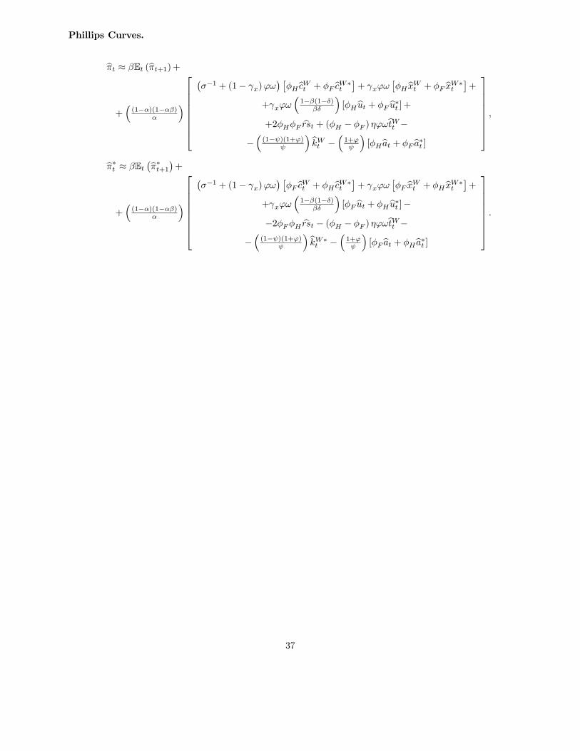
Phillips Curves.

bπt ≈ βEt (bπt+1)+

+³(1−α)(1−αβ)

α

´⎡⎢⎢⎢⎢⎢⎢⎢⎣

¡σ−1 + (1− γx)ϕω

¢ £φHbcWt + φFbcW∗t

¤+ γxϕω

£φHbxWt + φF bxW∗t

¤+

+γxϕω³1−β(1−δ)

βδ

´[φHbut + φF bu∗t ] +

+2φHφF brst + (φH − φF ) ηϕωbtWt −−³(1−ψ)(1+ϕ)

ψ

´bkWt − ³1+ϕψ ´[φHbat + φFba∗t ]

⎤⎥⎥⎥⎥⎥⎥⎥⎦,

bπ∗t ≈ βEt¡bπ∗t+1¢+

+³(1−α)(1−αβ)

α

´⎡⎢⎢⎢⎢⎢⎢⎢⎣

¡σ−1 + (1− γx)ϕω

¢ £φFbcWt + φHbcW∗t

¤+ γxϕω

£φF bxWt + φHbxW∗t

¤+

+γxϕω³1−β(1−δ)

βδ

´[φF but + φHbu∗t ]−

−2φFφH brst − (φH − φF ) ηϕωbtWt −−³(1−ψ)(1+ϕ)

ψ

´bkW∗t −³1+ϕψ

´[φFbat + φHba∗t ]

⎤⎥⎥⎥⎥⎥⎥⎥⎦.

37

Tables and Figures

Figure 1: Impulse Response Functions (Domestic Monetary Shock)

0 5 10 15 20-6

-5

-4

-3

-2

-1

0Real Exchange Rate (IAC)

%

0 5 10 15 20-6

-5

-4

-3

-2

-1

0Real Exchange Rate (CAC)

%

0 5 10 15 20-6

-5

-4

-3

-2

-1

0Real Exchange Rate (NAC)

%

0 5 10 15 20-2

-1.5

-1

-0.5

0Domestic Consumption (IAC)

%

0 5 10 15 20-2

-1.5

-1

-0.5

0Domestic Consumption (CAC)

%

0 5 10 15 20-2

-1.5

-1

-0.5

0Domestic Consumption (NAC)

%

0 5 10 15 20-4

-3

-2

-1

0Domestic Investment (IAC)

%

0 5 10 15 20-6

-5

-4

-3

-2

-1

0Domestic Investment (CAC)

%

0 5 10 15 20-10

-8

-6

-4

-2

0Domestic Investment (NAC)

%

Capital

No Capital

These graphs report the selected impulse response functions (IRFs) for each series given our parameterization. TheIRFs represent the response of endogenous variables to a one time, one standard deviation domestic monetaryshock innovation. ’Capital’ identifies a given variant of the model with capital, conditional on the choice of theadjustment cost function. NAC denotes the no adjustment cost case, CAC denotes the capital adjustment cost case(which is used in CKM, 2002), IAC denotes the investment adjustment cost case (our benchmark). ’No Capital’identifies the NoC model without capital, which offers an alternative where capital is not available and technologiesare linear-in-labor. We use Matlab 7.4.0 and Dynare v3.051 for the stochastic simulation.

38

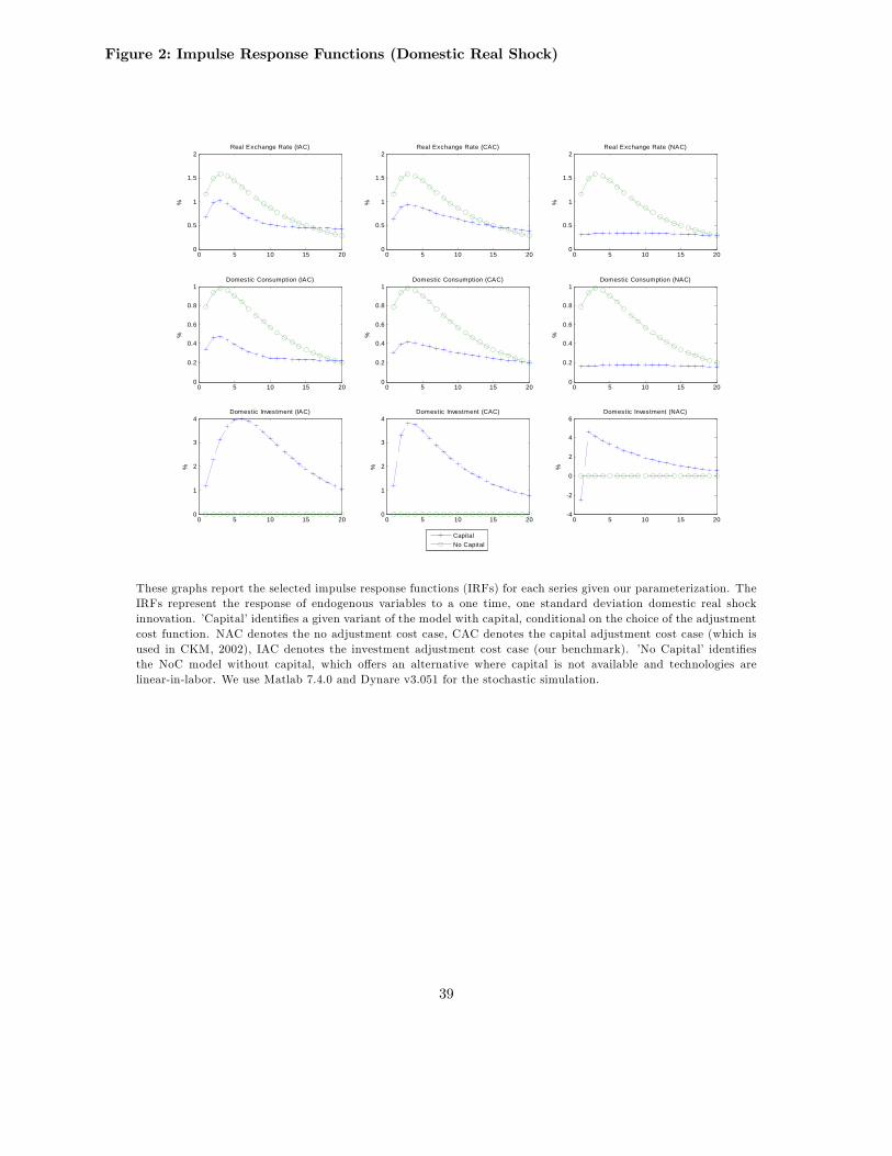
Figure 2: Impulse Response Functions (Domestic Real Shock)

0 5 10 15 200

0.5

1

1.5

2Real Exchange Rate (IAC)

%

0 5 10 15 200

0.5

1

1.5

2Real Exchange Rate (CAC)

%

0 5 10 15 200

0.5

1

1.5

2Real Exchange Rate (NAC)

%

0 5 10 15 200

0.2

0.4

0.6

0.8

1Domestic Consumption (IAC)

%

0 5 10 15 200

0.2

0.4

0.6

0.8

1Domestic Consumption (CAC)

%

0 5 10 15 200

0.2

0.4

0.6

0.8

1Domestic Consumption (NAC)

%

0 5 10 15 200

1

2

3

4Domestic Investment (IAC)

%

0 5 10 15 200

1

2

3

4Domestic Investment (CAC)

%

0 5 10 15 20-4

-2

0

2

4

6Domestic Investment (NAC)

%

Capital

No Capital

These graphs report the selected impulse response functions (IRFs) for each series given our parameterization. TheIRFs represent the response of endogenous variables to a one time, one standard deviation domestic real shockinnovation. ’Capital’ identifies a given variant of the model with capital, conditional on the choice of the adjustmentcost function. NAC denotes the no adjustment cost case, CAC denotes the capital adjustment cost case (which isused in CKM, 2002), IAC denotes the investment adjustment cost case (our benchmark). ’No Capital’ identifiesthe NoC model without capital, which offers an alternative where capital is not available and technologies arelinear-in-labor. We use Matlab 7.4.0 and Dynare v3.051 for the stochastic simulation.

39

Table 1: Parameters used for the Benchmark Calibration.

BenchmarkStructural Parameters:Discount Factor β = 0.99Elasticity of Intratemporal Substitution η = 1.5Elasticity of Substitution across Varieties θ = 10Elasticity of Intertemporal Substitution σ = 1/5(Inverse) Elasticity of Labor Supply ϕ = 3Home Bias Parameter φH = 0.94, φF = 0.06Calvo Price Stickiness Parameter α = 0.75Depreciation Rate δ = 0.021Capital/Investment Adjustment Cost χ =varies, κ =variesElasticity of Capital Utilization Cost λ = 5.80Labor Share ψ = 2/3Taylor Rule Parameters ρi = 0.85, ψπ = 2, ψy = 0.5

Exogenous Shock Parameters:Real Shock Parameters ρa = 0.9, σ (bεat ) =varies, σ (bεa∗t ) =varies, corr (bεat ,bεa∗t ) =variesMonetary Shock Parameters ρm = 0.9, σ (bεmt ) =varies, σ (bεm∗t ) =varies, corr (bεmt ,bεm∗t ) =variesInvestment Shock Parameters ρv = 0.9, σ (bεvt ) =varies, σ (bεv∗t ) =varies, corr (bεvt ,bεv∗t ) =varies

Composite Parameters:

Steady State Investment Share γx≡ (1−ψ)δ( θθ−1)(β−1−(1−δ))

= 0.203

Slope of the Phillips Curve (1−α)(1−αβ)α = 0.086

Strategic Complementarity on Cons. σ−1+(1− γx)ϕω = 8.987, ω ≡ϕψ2+(1−ψ)(1+ϕ)2ϕψ+(1−ψ)ψϕ2 = 1.667

Strategic Complementarity on Inv. γxϕω = 1.013, ω ≡ϕψ2+(1−ψ)(1+ϕ)2ϕψ+(1−ψ)ψϕ2 = 1.667

This table summarizes our parameterization. The more relevant comparison of our calibration is with CKM’s (2002) variant witha Taylor rule and Steinsson’s (2008) specification with homogeneous labor markets, even though Steinsson (2008) does not includecapital. The composite parameters are inferred based on the parametric choices described for our benchmark.

40

Table 2: Exchange Rates and Consumption.

Capital Specs. Variable Capital UtilizationVariable U.S. Data IAC NoC CAC NAC IAC+CU CAC+CU NAC+CU

Monetary ShocksStd. dev. to GDPConsumption 0.81 0.81 1.07 0.49 0.03 0.44 0.37 0.03RER 5.14 5.13 6.44 3.09 0.19 2.65 2.31 0.19

AutocorrelationConsumption 0.87 0.42 0.50 0.42 0.78 0.35 0.41 0.78RER 0.78 0.44 0.52 0.45 0.78 0.38 0.45 0.77

Cross-correlationConsumption 0.33 0.20 0.28 0.19 0.21 0.26 0.21 0.21

Real ShocksStd. dev. to GDPConsumption 0.81 0.39 0.91 0.35 0.15 0.41 0.35 0.13RER 5.14 1.64 3.14 1.51 0.56 1.72 1.53 0.52

AutocorrelationConsumption 0.87 0.82 0.84 0.84 0.75 0.82 0.84 0.75RER 0.78 0.84 0.85 0.85 0.76 0.84 0.85 0.76

Cross-correlationConsumption 0.33 0.65 0.76 0.64 0.70 0.65 0.62 0.70

Investment-Specific ShocksStd. dev. to GDPConsumption 0.81 0.39 − 0.40 0.37 0.43 0.41 0.37RER 5.14 1.63 − 1.79 1.93 1.77 1.85 1.94

AutocorrelationConsumption 0.87 0.96 − 0.96 0.70 0.95 0.96 0.70RER 0.78 0.96 − 0.93 0.70 0.97 0.94 0.70

Cross-correlationConsumption 0.33 0.65 − 0.59 0.45 0.65 0.59 0.45

Real + Monetary ShocksStd. dev. to GDPConsumption 0.81 0.57 1.00 0.44 0.05 0.42 0.37 0.05RER 5.14 3.12 5.23 2.46 0.25 2.35 2.05 0.25

AutocorrelationConsumption 0.87 0.53 0.60 0.58 0.76 0.50 0.58 0.76RER 0.78 0.50 0.57 0.55 0.77 0.48 0.55 0.77

Cross-correlationConsumption 0.33 0.41 0.45 0.39 0.54 0.38 0.38 0.54

This table reports the theoretical moments for each series given our parameterization. All statistics are computed aftereach simulated series is H-P filtered (smoothing parameter=1600). NAC denotes the no adjustment cost case, CAC denotesthe capital adjustment cost case (which is used in CKM, 2002), IAC denotes the investment adjustment cost case (ourbenchmark), +CU indicates that capital utilization has been added (as in Christiano et al., 2005), and NoC is the modelstripped from capital (similar to Steinsson, 2008). We use Matlab 7.4.0 and Dynare v3.051 for the stochastic simulation.

Data Sources: The OECD’s Quarterly National Accounts, OECD’s Economic Outlook, and OECD’s Main Economic Indica-tors are the most important data sources. Some series are complemented with data from the Bureau of Economic Analysis,the Bureau of Labor Statistics, the Federal Reserve System, the European Central Bank (ECB), and WM/Reuters. For moredetails, see the description of the dataset in the Appendix.

41

Table 3: Business Cycle Statistics (Monetary Shocks).

Capital Specs. Variable Capital UtilizationIAC NoC CAC NAC IAC+CU CAC+CU NAC+CU

Variable U.S. Data Monetary ShocksStd. dev.GDP∗ 1.54 1.54 1.54 1.54 1.54 1.54 1.54 1.54

Std. dev. to GDPEmployment 0.66 1.56 1.00 1.53 1.54 1.26 1.40 1.55Investment∗∗ 3.38 3.39 − 3.39 5.08 3.37 3.39 5.09Net Exports 0.25 0.40 0.21 0.25 0.17 0.30 0.22 0.17Exports 2.59 1.25 1.10 1.13 1.08 1.01 1.03 1.08Imports 3.31 3.54 1.79 2.21 1.46 2.60 1.90 1.47

AutocorrelationGDP 0.87 0.62 0.49 0.40 −0.05 0.75 0.52 −0.04Employment 0.92 0.64 0.49 0.40 −0.05 0.67 0.38 −0.05Investment 0.91 0.88 − 0.43 −0.04 0.84 0.42 −0.04Net Exports 0.83 0.86 0.70 0.69 0.21 0.86 0.67 0.21Exports 0.85 0.69 0.52 0.45 −0.03 0.72 0.44 −0.03Imports 0.84 0.87 0.70 0.70 0.20 0.86 0.67 0.21

Cross-correlationGDP∗ 0.44 0.44 0.46 0.44 0.45 0.44 0.44 0.44Employment 0.29 0.43 0.46 0.44 0.45 0.45 0.44 0.44Investment 0.33 0.02 − 0.24 0.30 0.10 0.25 0.29

CorrelationsGDP, Net Exp. −0.47 −0.45 −0.47 −0.46 −0.49 −0.49 −0.50 −0.50GDP, Exp. 0.41 0.20 0.34 0.29 0.36 0.22 0.29 0.34GDP, Imp. 0.82 0.62 0.79 0.73 0.88 0.68 0.78 0.88Exp., Imp. 0.21 −0.51 −0.13 −0.27 −0.00 −0.47 −0.24 −0.02

This table reports the theoretical moments for each series given our parameterization. All statistics are computed after eachsimulated series is H-P filtered (smoothing parameter=1600). NAC denotes the no adjustment cost case, CAC denotes thecapital adjustment cost case (which is used in CKM, 2002), IAC denotes the investment adjustment cost case (our benchmark),+CU indicates that capital utilization has been added (as in Christiano et al., 2005), and NoC is the model stripped fromcapital (similar to Steinsson, 2008). We use Matlab 7.4.0 and Dynare v3.051 for the stochastic simulation.

(*) We calibrate the volatility and correlation of monetary shock innovations to match the observed volatility and cross-countrycorrelation of GDP.(**) We calibrate the adjustment cost parameter, if the model specification affords us one, to match the observed volatility ofinvestment.

Data Sources: The OECD’s Quarterly National Accounts, OECD’s Economic Outlook, and OECD’s Main Economic Indicatorsare the most important data sources. Some series are complemented with data from the Bureau of Economic Analysis, theBureau of Labor Statistics, the Federal Reserve System, the European Central Bank (ECB), and WM/Reuters. For moredetails, see the description of the dataset in the Appendix.

42

Table 4: Business Cycle Statistics (Real Shocks).

Capital Specs. Variable Capital UtilizationIAC NoC CAC NAC IAC+CU CAC+CU NAC+CU

Variable U.S. Data Real ShocksStd. dev.GDP∗ 1.54 1.54 1.54 1.54 1.54 1.54 1.54 1.54

Std. dev. to GDPEmployment 0.66 1.61 1.96 1.32 1.50 1.64 1.32 1.47Investment∗∗ 3.38 3.38 − 3.33 4.60 3.39 3.38 4.50Net Exports 0.25 0.17 0.34 0.15 0.10 0.18 0.15 0.10Exports 2.59 0.89 0.86 0.90 1.00 0.90 0.91 0.97Imports 3.31 2.25 3.77 2.04 1.25 2.30 2.06 1.22

AutocorrelationGDP 0.87 0.91 0.85 0.89 0.54 0.91 0.90 0.53Employment 0.92 0.48 0.61 0.32 −0.10 0.48 0.31 −0.10Investment 0.91 0.94 − 0.88 0.41 0.94 0.89 0.40Net Exports 0.83 0.84 0.92 0.85 −0.12 0.85 0.85 −0.13Exports 0.85 0.91 0.83 0.88 0.47 0.91 0.88 0.46Imports 0.84 0.86 0.91 0.87 0.43 0.87 0.87 0.41

Cross-correlationGDP∗ 0.44 0.44 0.46 0.44 0.46 0.44 0.44 0.46Employment 0.29 0.47 0.60 0.40 0.42 0.47 0.39 0.42Investment 0.33 0.57 − 0.56 0.38 0.57 0.54 0.38

CorrelationsGDP, Net Exp. −0.47 0.49 0.51 0.50 −0.18 0.48 0.50 −0.19GDP, Exp. 0.41 0.64 0.81 0.63 0.47 0.64 0.62 0.47GDP, Imp. 0.82 −0.15 −0.31 −0.11 0.53 −0.14 −0.12 0.54Exp., Imp. 0.21 0.61 0.27 0.66 0.55 0.60 0.67 0.54

This table reports the theoretical moments for each series given our parameterization. All statistics are computed after eachsimulated series is H-P filtered (smoothing parameter=1600). NAC denotes the no adjustment cost case, CAC denotes thecapital adjustment cost case (which is used in CKM, 2002), IAC denotes the investment adjustment cost case (our benchmark),+CU indicates that capital utilization has been added (as in Christiano et al., 2005), and NoC is the model stripped fromcapital (similar to Steinsson, 2008). We use Matlab 7.4.0 and Dynare v3.051 for the stochastic simulation.

(*) We calibrate the volatility and correlation of real shock innovations to match the observed volatility and cross-countrycorrelation of GDP.(**) We calibrate the adjustment cost parameter, if the model specification affords us one, to match the observed volatility ofinvestment.

Data Sources: The OECD’s Quarterly National Accounts, OECD’s Economic Outlook, and OECD’s Main Economic Indicatorsare the most important data sources. Some series are complemented with data from the Bureau of Economic Analysis, theBureau of Labor Statistics, the Federal Reserve System, the European Central Bank (ECB), and WM/Reuters. For moredetails, see the description of the dataset in the Appendix.

43

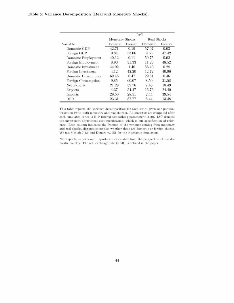
Table 5: Variance Decomposition (Real and Monetary Shocks).

IACMonetary Shocks Real Shocks

Variable Domestic Foreign Domestic ForeignDomestic GDP 42.71 0.19 57.07 0.03Foreign GDP 9.84 33.06 9.68 47.42Domestic Employment 40.12 0.11 59.75 0.02Foreign Employment 8.90 31.33 11.26 48.52Domestic Investment 44.92 1.40 53.40 0.28Foreign Investment 4.12 42.20 12.72 40.96Domestic Consumption 69.46 0.47 29.61 0.46Foreign Consumption 9.85 60.07 8.50 21.58Net Exports 21.29 52.76 7.46 18.49Exports 4.37 54.47 16.76 24.40Imports 29.50 28.51 2.44 39.54RER 23.31 57.77 5.44 13.48

This table reports the variance decomposition for each series given our parame-terization (with both monetary and real shocks). All statistics are computed aftereach simulated series is H-P filtered (smoothing parameter=1600). IAC denotesthe investment adjustment cost specification, which is our specification of refer-ence. Each column indicates the fraction of the variance coming from monetaryand real shocks, distinguishing also whether these are domestic or foreign shocks.We use Matlab 7.4.0 and Dynare v3.051 for the stochastic simulation.

Net exports, exports and imports are calculated from the perspective of the do-mestic country. The real exchange rate (RER) is defined in the paper.

44