Federal Reserve Bank of Dallas Globalization and Monetary Policy Institute

Working Paper No. 17 http://www.dallasfed.org/assets/documents/institute/wpapers/2008/0017.pdf

The Real Exchange Rate in Sticky Price Models: Does Investment

Matter?*

Enrique Martinez-Garcia Federal Reserve Bank of Dallas

Jens Søndergaard Bank of England

July 2008

Abstract This paper re-examines the ability of sticky-price models to generate volatile and persistent real exchange rates. We use a DSGE framework with pricing-to-market akin to those in Chari, et al. (2002) and Steinsson (2008) to illustrate the link between real exchange rate dynamics and what the model assumes about physical capital. We show that adding capital accumulation to the model facilitates consumption smoothing and significantly impedes the model’s ability to generate volatile real exchange rates. Our analysis, therefore, caveats the results in Steinsson (2008) who shows how real shocks in a sticky-price model without capital can replicate the observed real exchange rate dynamics. Finally, we find that the CKM (2002) persistence anomaly remains robust to several alternative capital specifications including set-ups with variable capital utilization and investment adjustment costs (see, e.g., Christiano, et al., 2005). In summary, the PPP puzzle is still very much alive and well. JEL codes: F31, F37, F41

* Enrique Martinez-Garcia, Research Department, Federal Reserve Bank of Dallas, 2200 N. Pearl Street, Dallas, TX 75201. +1 (214) 922- 5262. enrique.martinez-garcia@dal.frb.org. Jens Søndergaard, Monetary Instruments and Markets Division, Monetary Analysis, Bank of England. Threadneedle Street, London EC2R 8AH, UK. +44 (0)20 7601-4869. jens.sondergaard@bankofengland.co.uk. We would like to thank Mark Astley, Charles Engel, Alberto Musso, Roman Sustek, Jian Wang, Mark Wynne, Wenjuan Xie, and many seminar and conference participants at the Midwest Macro Meetings 2008 for helpful discussions. We also acknowledge the excellent research assistance provided by Artis Frankovics, and the support of the Federal Reserve Bank of Dallas and the Bank of England. All remaining errors are ours alone. The views in this paper do not necessarily reflect the views of the Bank of England, Federal Reserve Bank of Dallas or the Federal Reserve System.

1 Introduction

Understanding the short-run dynamics of real exchange rates remains a key issue on the open economy

research agenda. Standard international macro models have had difficulty replicating real exchange rates

that are both very volatile and highly persistent in the data. One recent strand of research has revived the

Dornbusch (1976a, 1976b) ‘exchange rate overshooting’ hypothesis arguing that exchange rate volatility is

essentially driven by monetary shocks interacting with sticky prices. For instance, Chari, et al. (2002) (CKM)

have shown how a two-country sticky-price model with pricing-to-market driven by monetary shocks has the

potential to simultaneously match the volatility of U.S. output and real exchange rates, hence resolving the

so-called international pricing puzzle. But their model does not reproduce the persistence of real exchange

rates and, thus, fails to address the persistence anomaly. Steinsson (2008), however, appears to resolve both

the international pricing puzzle and the persistence anomaly (jointly referred to as the PPP puzzle) with

real shocks and a sticky-price model with no capital.

In this paper, we use a DSGE framework akin to those in CKM (2002) and Steinsson (2008) to illustrate

the link between real exchange rate dynamics and what the model assumes about capital. We find that

omitting capital is not inconsequential in terms of the model’s ability to resolve the PPP puzzle. Our

benchmark model featuring complete asset markets, capital accumulation and investment adjustment costs

matches the real exchange rate persistence with real shocks, but generates less real exchange rate volatility

relative to a similar setup without capital. Furthermore, the same benchmark model replicates the observed

real exchange volatility with monetary policy shocks, but not the persistence.

In other words, for real shocks, our benchmark reverses some of the promising results presented by

Steinsson (2008) on the international pricing puzzle; for monetary shocks, it confirms the persistence anomaly

discussed by CKM (2002) as a robust fact. A first-pass reading of our results suggests that adding capital

to a sticky-price model takes us effectively "back to square one" in terms of resolving the PPP puzzle.

To understand our results, we must consider the role of capital accumulation in an open-economy model.

Access to capital accumulation facilitates intertemporal consumption smoothing, since it allows households

to adjust their investment-savings margin in response to country-specific shocks. Adjusting through the

intertemporal margin has the potential to generate a very smooth series for consumption and the real

exchange rate.

However, the ability to smooth consumption hinges on how costly it is for households to adjust their

capital stock. To illustrate this, our benchmark specification introduces investment adjustment costs similar

to those in Christiano, et al. (2005). The adjustment costs regulate the volatility of investment, but also

affect the volatility and cross-correlation of consumption. A direct implication of the complete asset markets

assumption is that consumption and the real exchange rate are linked together in the model. Adjustment

costs make it more costly to smooth consumption through the intertemporal margin, hence consumption

and (by extension) the real exchange rate become more volatile.

Capital utilization offers a way for households to get around the investment constraints imposed by the

adjustment costs. We show that adding capital utilization to the model as in Christiano, et al. (2005)

facilitates further consumption smoothing which, in turn, reduces the model’s ability to produce highly

volatile real exchange rates. Low real exchange rate volatility is also robust after the inclusion of investment-

specific shocks as in Greenwood, et al. (1988). While Justiniano and Primiceri (2008) have highlighted the

importance of these shocks in a closed economy setting, our benchmark calibration suggests that the same

1

shocks cannot fully account for consumption and real exchange rate volatilities in an open-economy setting.

So resolving the international pricing puzzle remains challenging.

Addressing the CKM (2002) persistence anomaly is not easy either. Our results suggest that the per-

sistence anomaly in response to monetary shocks is robust to adding capital back into the model, to the

specification of the adjustment cost function, and even to the addition of capital utilization. High persistence

is easier to get from real shocks since they trigger an endogenous monetary policy reaction that implies a

hump-shaped consumption response. As shown by Steinsson (2008), this hump-shaped response is important

to produce high real exchange rate persistence. But our paper argues that with real shocks is rather difficult

to match the volatility of the real exchange rate, if the model features capital.

In our view, the PPP puzzle is still very much alive and well in the context of the open-economy, sticky-

price model. Our results suggest that models without capital tend to suffer from a ‘volatility bias’ that

understates the true magnitude of the international pricing puzzle. Tackling the PPP puzzle requires a

two-pronged modelling strategy. The first prong is to build a model with capital that can generate very

volatile real exchanges rates stemming from a combination of real and other shocks (including monetary

policy shocks). The second prong entails looking for ways to ensure sufficient persistence.

Therefore, the key challenge is to find open-economy models that clearly break the link between the

real exchange rates and real quantities (particularly, consumption). Recent research has presented various

options including informational frictions (e.g., Martínez-García, 2008), asymmetric price stickiness (e.g.,

Benigno, 2004, Carvalho and Nechio, 2008), asymmetric monetary policy rules (e.g., Groen and Matsumoto,

2004), alternative financial market structures (e.g., Heathcote and Perri, 2002), and co-integrated, unit-root

technology shocks (e.g., Rabanal, et al., 2008). Future research may need to incorporate some of these

features and further re-examine the ability of the open-economy, sticky-price framework to generate volatile

and persistent real exchange rates as well as realistic business cycles.

The paper is structured as follows. Section 2 contains a description of our two-country model with capital

accumulation, while section 3 outlines our calibration strategy for the simulations. Section 4 summarizes

the quantitative findings, and section 5 the sensitivity analysis. Section 6 concludes.

2 The Open Economy Model

Here, we describe the model and the log-linearized equilibrium conditions simultaneously. As a notational

convention, any variable identified with lower-case letters and a caret on top represents a transformation

(expressed in log deviations relative to steady state) of the corresponding variable in upper-case letters. See

the companion working paper (Martínez-García and Søndergaard, 2008) for more details on the equilibrium

conditions, and the log-linearization approach.

2.1 The Intertemporal Consumption and Savings Problem

We specify a stochastic, two-country general equilibrium model. Each country is populated by a continuum

of infinitely lived (and identical) households in the interval [0, 1]. In each period, the domestic household’s

utility function is additively separable in consumption, Ct, and labor, Lt. Domestic households maximize,

X∞

τ=0βτEt

∙1

1− σ−1(Ct+τ )

1−σ−1 − 1

1 + ϕ(Lt+τ )

1+ϕ

¸, (1)

2

where β ∈ (0, 1) is the subjective intertemporal discount factor. The elasticity of intertemporal substitutionsatisfies that σ > 0 (σ 6= 1), while the inverse of the Frisch elasticity of labor supply satisfies that ϕ > 0.

We assume that households in either country have unrestricted access to a complete set of contingent

claims, traded internationally. The domestic household maximizes its lifetime utility in (1) subject to the

sequence of budget constraints described by,

Pt (Ct +Xt) + Et [Mt,t+1Bt+1] ≤ Bt +WtLt + ZtKt, (2)

and the law of motion for physical capital,

Kt+1 = (1− δ)Kt + VtΦ (Xt,Xt−1,Kt)Xt, (3)

where Bt+1 is the nominal payoff in period t+ 1 of the portfolio held at the end of period t. The portfolio

includes a proportional share on the nominal profits generated by the domestic firms, since sole ownership

of the domestic firms rests in the hands of the domestic households. Mt,t+1 is the stochastic discount factor

(SDF) for one-period ahead nominal payoffs relevant to the domestic household.

Money plays the role of a unit of account only. Wt is the domestic nominal wage, Pt is the domestic

consumption price index (CPI), and Zt defines the nominal return on capital. Moreover, Xt is domestic

real investment, Kt stands for domestic physical capital (or capital services) in real terms1, and Vt is an

investment-specific shock as in Greenwood, et al. (1988). The foreign households maximize their lifetime

utility subject to an analogous sequence of budget constraints and a law of motion for capital.

Besides investigating the role of investment-specific shocks to the law of motion in (3), we also assume

that capital accumulation is subject to adjustment costs Φ (·) . We adopt the investment adjustment cost(IAC) function used by Christiano, et al. (2005) and Groth and Kahn (2007) as our benchmark. The IAC

function takes the following form2,

Φ

µXt

Xt−1

¶= 1− 1

2κ

³Xt

Xt−1− 1´2

Xt

Xt−1

, (4)

where Xt

Xt−1denotes the gross investment growth rate. In steady state, the investment adjustment costs dis-

sipate, investment is constant, and the investment-to-capital ratio is equal to the depreciation rate as posited

in the standard neoclassical model. The same adjustment cost formula applies to the foreign household’s

problem.

Aggregation Rules and the Price Indexes. We assume that investment, like consumption, is a com-

posite index of domestic and imported foreign varieties3 . The home and foreign consumption bundles of the

1The distinction between physical capital and capital services only becomes relevant when we introduce differences in thecapital utilization rate. Until then, we use both concepts interchangeably.

2Among the properties of this adjustment cost function that are relevant for us, we note that in steady state Φ (1) = 1,Φ0 (1) = 0, and Φ00 (1) = −κ. For more details, see the companion working paper (Martínez-García and Søndergaard, 2008).

3Aggregate investment goods can only be used by local firms after aggregation. However, local and foreign varieties of goodscan be traded internationally for either consumption or investment purposes.

3

domestic household, CHt and CF

t , as well as the investment bundles, XHt and XF

t , are aggregated by means

of a CES preference index as,

CHt =

∙Z 1

0

Ct (h)θ−1θ dh

¸ θθ−1

, CFt =

∙Z 1

0

Ct (f)θ−1θ df

¸ θθ−1

, (5)

XHt =

∙Z 1

0

Xt (h)θ−1θ dh

¸ θθ−1

, XFt =

∙Z 1

0

Xt (f)θ−1θ df

¸ θθ−1

, (6)

while domestic aggregate consumption and investment, Ct and Xt, are defined with another CES preference

index as,

Ct =

∙φ1η

H

¡CHt

¢ η−1η + φ

1η

F

¡CFt

¢ η−1η

¸ ηη−1

, (7)

Xt =

∙φ1η

H

¡XHt

¢ η−1η + φ

1η

F

¡XFt

¢ η−1η

¸ ηη−1

. (8)

The elasticity of substitution across varieties produced within a country is θ > 1, and the elasticity of

intratemporal substitution between the home and foreign bundles of varieties is η > 0. The share of the

home goods in the domestic aggregator is φH , while the share of foreign goods is φF . We assume the shares

are homogeneous, i.e. φH + φF = 1. Similarly, we define the aggregators for the foreign household. We

introduce home bias in preferences (e.g., Warnock, 2003), as well as in the composition of investment, by

requiring the shares to satisfy that φ∗H = φF and φ∗F = φH .

The symmetry of the aggregators implies that the relative price between consumption and investment

goods is one, as implied by equation (2). Given standard results on functional separability, the indexes which

correspond to our specification of aggregators for the CPIs are,

Pt =hφH

¡PHt

¢1−η+ φF

¡PFt

¢1−ηi 11−η

, (9)

and,

PHt =

∙Z 1

0

Pt (h)1−θ

dh

¸ 11−θ

, PFt =

∙Z 1

0

Pt (f)1−θ

df

¸ 11−θ

, (10)

where PHt and PF

t are the price sub-indexes for the home- and foreign-produced bundle of goods in units of

the home currency. Similarly for the foreign CPI, P ∗t , and the foreign price sub-indexes, PH∗t and PF∗

t . We

define the real exchange rate as,

RSt ≡StP

∗t

Pt, (11)

where St denotes the nominal exchange rate.

Consumption, Savings and Investment. Aggregate consumption in each country evolves according to

a pair of standard Euler equations,

bct ≈ Et [bct+1]− σ³bit − Et [bπt+1]´ , (12)

bc∗t ≈ Et£bc∗t+1¤− σ

³bi∗t − Et £bπ∗t+1¤´ , (13)

4

while the perfect international risk-sharing condition implies that,

bct − bc∗t ≈ σ brst. (14)

Equations (12) − (14) are well-known in the literature. The intertemporal elasticity of substitution, σ,

regulates the sensitivity of the consumption path to real interest rates and to the real exchange rate. Equation

(14), in particular, establishes a positive relationship between the real exchange rate and relative consumption

across countries. Consequently, domestic consumption becomes relatively high whenever it is relatively

‘cheap’.

Under the investment adjustment cost function (IAC), capital accumulation evolves according to the

same law of motion,

bkt+1 ≈ (1− δ)bkt + δ (bxt + bvt) , (15)bk∗t+1 ≈ (1− δ)bk∗t + δ (bx∗t + bv∗t ) , (16)

where bkt and bk∗t denote physical capital, bxt and bx∗t stand for investment, and bvt and bv∗t are the investment-specific shocks. Moreover, the household’s optimal asset pricing and investment decisions imply the following

pair of equations in the home country,

bqt ≈ (1− δ)βEt [bqt+1] + h(1− (1− δ)β)Et¡brzt+1¢− ³bit − Et [bπt+1]´i , (17)

bxt ≈ 1

1 + βbxt−1 + β

1 + βEt [bxt+1] + 1

κ (1 + β)(bqt + bvt) , (18)

and the analogous pair for the foreign country,

bq∗t ≈ (1− δ)βEt£bq∗t+1¤+ h(1− (1− δ)β)Et

¡brz∗t+1¢− ³bi∗t − Et £bπ∗t+1¤´i , (19)

bx∗t ≈ 1

1 + βbx∗t−1 + β

1 + βEt£bx∗t+1¤+ 1

κ (1 + β)(bq∗t + bv∗t ) , (20)

where bqt and bq∗t are the real shadow prices of an additional unit of investment (or Tobin’s q), and brzt+1 ≡bzt+1− bpt+1 and brz∗t+1 ≡ bz∗t+1− bp∗t+1 denote the real returns on capital. The investment-specific shocks bvt andbv∗t follow AR (1) processes of the form,

bvt = ρvbvt−1 + bεvt , |ρv| < 1, (21)bv∗t = ρvbv∗t−1 + bεv∗t , |ρv| < 1, (22)

where bεvt and bεv∗t are zero mean, and normally-distributed innovations.

The asset pricing equations in (17) and (19) can be interpreted as a pair of financial arbitrage equations

between real interest rates and real returns on capital. The parameter κ regulates the degree of concavity

of the IAC function around the steady state. It directly affects the sensitivity of investment to either

investment-specific shocks or fluctuations in Tobin’s q through the investment equations in (18) and (20).

The investment equations introduce an element of inertia in investment captured by the lagged term, but also

ensure that investment becomes forward-looking. Choosing the level of investment today sets the base for

5

investment growth tomorrow and, therefore, affects next period’s adjustment costs. Under this adjustment

cost specification, the investment response to the shadow value of capital services (Tobin’s q) may not be

instantaneous.

2.2 The Price-Setting Problem under Sticky Prices

There is a continuum of firms located in the interval [0, 1] in each country. Each firm produces a differentiated,

tradable good, supplies the home and foreign market, and sets prices in the local currency (henceforth, LCP

pricing). Re-selling is infeasible across markets and, furthermore, each firm enjoys monopolistic power in its

own variety. We introduce nominal rigidities à la Calvo (1983). With probability α ∈ (0, 1) in each period,the firm maintains its previous period prices in both markets unchanged. However, with probability (1− α),

the firm optimally resets its prices.

We assume that production is based on a Cobb-Douglas technology, i.e. for every firm h ∈ [0, 1],

Yt (h) = At (Kt (h))1−ψ (Lt (h))

ψ , (23)

where At is an aggregate productivity shock in the home country. The labor share in the production function

is pinned down by ψ ∈ (0, 1), while (23) reduces to the linear in labor case if ψ = 1. An identical technologyis used by foreign firms, but subject to a foreign-specific aggregate productivity shock A∗t .

Solving the cost-minimization problem of each individual domestic firm yields an efficiency condition

linking the capital-to-labor ratio to the factor price ratio as follows,

Kt (h)

Lt (h)=1− ψ

ψ

Wt

Zt, (24)

for all h ∈ [0, 1], as well as a characterization for the domestic nominal marginal costs,

MCt =1

At

1

ψψ (1− ψ)1−ψ(Wt)

ψ(Zt)

1−ψ. (25)

Both factors, labor and capital, are homogenous within a country and immobile across borders. Factor

markets are also perfectly competitive. Therefore, wages and the returns on capital equalize in each country

(but not necessarily across countries), as implied in (24) and (25).

Since the production function is of constant returns to scale, all local firms choose the same capital-to-

labor ratio and confront the same marginal costs even though they may end up producing different amounts.

An analogous efficiency condition and nominal marginal cost function can be derived for the foreign firms.

The Optimal Pricing Problem. A re-optimizing domestic firm h chooses a domestic and a foreign price,ePt (h) and eP ∗t (h), to maximize the expected discounted value of its net profits,X∞

τ=0EtnατMt,t+τ

h³ eCt,t+τ (h) + eXt,t+τ (h)´³ ePt (h)−MCt+τ

´+³ eC∗t,t+τ (h) + eX∗t,t+τ (h)´³St+τ eP ∗t (h)−MCt+τ

´io,

(26)

6

where Mt,t+τ ≡ βτ³Ct+τCt

´−σ−1Pt

Pt+τis the SDF for τ -periods ahead nominal payoffs corresponding to the

domestic household, subject to a pair of demand constraints in each goods market,

eCt,t+τ (h) + eXt,t+τ (h) =

à ePt (h)PHt+τ

!−θ ¡CHt+τ +XH

t+τ

¢, (27)

eC∗t,t+τ (h) + eX∗t,t+τ (h) =

à eP ∗t (h)PH∗t+τ

!−θ ¡CH∗t+τ +XH∗

t+τ

¢, (28)

where eCt,t+τ (h) and eC∗t,t+τ (h) indicate the consumption demand for any variety h ∈ [0, 1] at home andabroad respectively, given that prices ePt (h) and eP ∗t (h) remain unchanged between time t and t + τ . Sim-

ilarly, eXt,t+τ (h) and eX∗t,t+τ (h) indicate the household’s investment demand. The problem is solved under

the implicit assumption that firms must supply the domestic and foreign markets with as much of the

consumption-investment good as it is demanded at the current prices (rationing is not allowed). We derive

the demand for variety h in the home and foreign markets in the companion working paper (Martínez-García

and Søndergaard, 2008).

The problem of the re-optimizing foreign firm f is to maximize the expected discounted value of its net

profits subject to a similar pair of demand constraints.

Pricing Dynamics. The efficiency conditions that relate the capital-to-labor ratio to the factor price ratio

in each country, as described by equations (24) and its foreign counterpart, can be summarized as,

brzt ≈ 1

σbct + 1 + ϕ

ψbyt −µ1 + (1− ψ)ϕ

ψ

¶bkt − 1 + ϕ

ψbat, (29)

brz∗t ≈ 1

σbc∗t + 1 + ϕ

ψby∗t −µ1 + (1− ψ)ϕ

ψ

¶bk∗t − 1 + ϕ

ψba∗t , (30)

which already substitute out both labor and wages. Households equate the marginal rate of substitution

between consumption and labor to real wages. The Cobb-Douglas technology allows us to substitute out

labor in the expression for real wages, and to link the capital-to-labor ratio to productivity and the capital-

to-output ratio. Equations (29) and (30) are the result of re-arranging the firms’ efficiency conditions along

these lines, so that we can express the real return on capital as proportional to the real wages and the capital-

to-labor ratio. Total output supply is obtained by aggregating the Cobb-Douglas production function over

all local firms and log-linearizing, i.e.

byt ≈ bat + (1− ψ)bkt + ψblt, (31)by∗t ≈ ba∗t + (1− ψ)bk∗t + ψbl∗t . (32)

The productivity shocks bat and ba∗t follow AR (1) processes of the form,

bat = ρabat−1 + bεat , |ρa| < 1, (33)ba∗t = ρaba∗t−1 + bεa∗t , |ρa| < 1, (34)

where bεat and bεa∗t are zero mean, and normally-distributed innovations.

7

Total output demand can be approximated as,

byt ≈ ηbtWt + (1− γx)bcWt + γxbxWt , (35)by∗t ≈ −ηbtWt + (1− γx)bcW∗t + γxbxW∗t , (36)

where the superscriptsW andW ∗ denote the following weighted averages for consumption, bcWt ≡ φHbct+φFbc∗tand bcW∗t ≡ φFbct + φHbc∗t . Similarly, for investment and for other price indexes. We define world terms oftrade as btWt ≡ bpF,W∗t − bpW∗t , implying that an increase in btWt shifts consumption and investment spending

away from the foreign goods and into the domestic goods.

The inflation dynamics in the model can be derived as follows,

bπt ≈ βEt (bπt+1)++³(1−α)(1−αβ)

α

´⎡⎢⎢⎣¡σ−1 + (1− γx)ϕω

¢ £φHbcWt + φFbcW∗t

¤+ γxϕω

£φHbxWt + φF bxW∗t

¤+

+2φHφF brst + (φH − φF ) ηϕωbtWt −−³(1−ψ)(1+ϕ)

ψ

´bkWt − ³1+ϕψ ´[φHbat + φFba∗t ]

⎤⎥⎥⎦ , (37)bπ∗t ≈ βEt

¡bπ∗t+1¢++³(1−α)(1−αβ)

α

´⎡⎢⎢⎣¡σ−1 + (1− γx)ϕω

¢ £φFbcWt + φHbcW∗t

¤+ γxϕω

£φF bxWt + φHbxW∗t

¤+

−2φFφH brst − (φH − φF ) ηϕωbtWt −−³(1−ψ)(1+ϕ)

ψ

´bkW∗t −³1+ϕψ

´[φFbat + φHba∗t ]

⎤⎥⎥⎦ , (38)

where ω ≡³ϕψ2+(1−ψ)(1+ϕ)2ϕψ+(1−ψ)ψϕ2

´is a composite parameter, and the investment share in steady state is given

by γx ≡ (1− ψ) δh³

θθ−1

´ ¡β−1 − (1− δ)

¢i−1. This characterization requires us to include an additional

equation to pin down the world terms of trade, btWt , i.e.∆btWt − βEt

¡∆btWt+1¢+µ(1− α) (1− αβ)

α

¶btWt ≈ φHφFφH − φF

∙µ(1− α) (1− αβ)

α

¶ brst − bπRt + βEt³bπRt+1´¸ .

(39)

Changes in world terms of trade are defined as ∆btWt ≡ btWt −btWt−1, and the relative inflation as bπRt ≡ bπt− bπ∗t .Equation (39) is necessary because the relative price effects on inflation cannot be fully summarized by the

real exchange rate, except in the special case where there is no home bias (i.e. φH = φF ). Moreover, they

are also necessary to determine the total output demand in (35)− (36)4 .The first three terms inside the brackets in (37)−(38) reveal the effects of aggregate demand for consump-

tion and investment. Adding capital requires firms to produce not only to satisfy consumption demand, but

also investment demand and, naturally, that drives factor prices and inflation up. However, the sensitivity

of the real marginal cost to different demand pressures varies as a function of the intertemporal elasticity of

substitution, σ, the inverse of the Frisch labor supply elasticity, ϕ, the labor share, ψ, and also the investment

share in steady state, γx.

The next two terms reflect the impact of expenditure-switching across countries through relative price

adjustments on inflation. Real exchange rates do part of the adjustment in this model, but they are not the

4 If we take consumption to be the target of monetary policy, as Steinsson (2008) does, and assume no home bias, an equationfor world terms of trade is no longer necessary to close the model.

8

only relative price to do so under home bias (i.e., if φH 6= φF ). The world terms of trade contributes to

explain changes in the demand for home- and foreign-produced goods which cannot be accounted by the real

exchange rate. However, real exchange rates and world terms of trade are tied together in equation (39).

The remaining two terms in (37)− (38) have to do with the effect of real shocks on the real marginal cost,and the role of the efficiency conditions5.

2.3 Monetary Policy and Trade Patterns

The Taylor rule is often viewed as the trademark of modern monetary policy. We consider policy rules for

the short-term nominal interest rate of the type proposed by Taylor (1993)6,

bit = ρibit−1 + (1− ρi)£ψπbπt + ψybyt¤+ bmt, (40)bi∗t = ρibi∗t−1 + (1− ρi)£ψπbπ∗t + ψyby∗t ¤+ bm∗t , (41)

where bmt and bm∗t define the monetary shocks, and bit and bi∗t are the corresponding monetary policy instru-ments. Also, bπt ≡ bpt − bpt−1 and bπ∗t ≡ bp∗t − bp∗t−1 are the (gross) CPI inflation rates, and byt and by∗t denotethe aggregate output.

The policy rules reflect the assumption that monetary authorities face a trade-off between inflation and

output. In line with most of the literature, we assume that monetary authorities smooth changes in the

actual short-term nominal interest rates, bit and bi∗t . But a discretionary component to monetary policy is stillpresent. Several interpretations can be given to the monetary shocks. They may reflect the central bank’s

failure to keep the interest rate at the level prescribed by the rule, or they might capture deliberate decisions

to deviate transitorily from a systematic rule (see, e.g., Clarida, et al., 1998, 2000). It may even capture

random shifts in the output potential of the economy, if the central bank targets a measure of output gap

rather than output itself. Hence, bmt and bm∗t are more than discretionary policy shocks. Keeping that inmind, the monetary shocks bmt and bm∗t are modelled as exogenous AR (1) processes of the form,

bmt = ρm bmt−1 + bεmt , |ρm| < 1, (42)bm∗t = ρm bm∗t−1 + bεm∗t , |ρm| < 1, (43)

where bεmt and bεm∗t are zero mean, and normally-distributed innovations.

Real Imports, Real Exports, and the Net Exports Share. In a two-country model, it suffices to

determine the trade patterns from the perspective of the domestic country. The equations for domestic real

5The evolution of relative factor prices, which in our model is the evolution of wages relative to the rental rate of capital,would determine the willingness of firms to become more or less capital-intensive. Capital appears in the marginal cost structureto account, at least partially, for the effeciency gains in the factor allocation.

6 Steinsson (2008) experiments with a rule that targets consumption rather than output. In a model without capital, thedifference between output and consumption is given by net exports.

9

exports and real imports can be log-linearized as,

dexpt ≈ ηφHφFbtWt − ηφH

³bpF,Rt − bpRt ´+ (1− γx)bc∗t + γxbx∗t , (44)

dimpt ≈ −ηbtWt − ηφH

³bpF,Rt − bpRt ´+ (1− γx)bct + γxbxt. (45)

In order to determine the evolution of both imports and exports, we need to add an additional equation

from the pricing dynamics of the firms, i.e.

bπF,Rt − βEt³bπF,Rt+1

´+

µ(1− α) (1− βα)

α

¶³bpF,Rt − bpRt ´ ≈ µ(1− α) (1− βα)

α

¶ brst, (46)

where bπF,Rt ≡ bpF,Rt − bpF,Rt−1 and bpF,Rt ≡ bpFt − bpF∗t represent relative price on foreign goods, while bpRt ≡ bpt− bp∗tis the relative CPI. These three equations indicate that the strength of the demand for consumption and

investment purposes has a major impact on both exports and imports. They also tells us that exports and

imports depend on world terms of trade, btWt , and indirectly on the real exchange rate, brst, and the relativeCPI, bpRt . The sensitivity to world terms of trade differs between exports and imports, reflecting the effectof the home bias assumption.

Let us denote the deviation of the share of net exports over GDP from its steady state as btbt. Then, thetrade balance is easily computed as the difference between domestic output and domestic consumption plus

investment in real terms (the domestic absorption) (see, e.g., Galí and Monacelli, 2005), i.e.

btbt ≡ byt − (1− γx)bct − γxbxt.Using the formula for total output demand in (35), we derive the following characterization for the share of

real net exports7 ,

btbt ≈ ηbtWt − (1− γx)φF (bct − bc∗t )− γxφF (bxt − bx∗t ) = φF

³dexpt −dimpt

´, (47)

where the second equality follows from the perfect international risk-sharing condition in (14). All relative

price effects on the trade balance are subsumed in our measure of world terms of trade, btWt .2.4 The Benchmark and Other Specifications

The core of the model consists of three blocks of equations. The first block has two Euler equations (equa-

tions (12) − (13)) and the perfect international risk-sharing condition (equation (14)) to characterize theconsumption-savings decisions of households. It has a pair of asset pricing equations for Tobin’s q coupled

with two investment equations (equations (17)− (20)) for the capital-investment decisions. We also add twomore equations for the law of motion of capital in the domestic and foreign countries (equations (15)− (16)).The second block adds three more equations to define the dynamics of inflation at home and abroad as

well as a measure of world terms of trade (equations (37)− (39)). This block also includes a pair of efficiencyconditions that constraint the real returns on capital (equations (29) − (30)), and two more equations to

7 In steady state, the real trade balance is zero by assumption. Nonetheless, exchanges do occur between the two countriesand the parameter φF represents the steady state share of imports for consumption and investment purposes relative to output.

10

describe the total output demand in both countries (equations (35) − (36)). The third and final blocksummarizes the role of the monetary authorities with a pair of monetary policy rules (equations (40)− (41)).We complete the core of the model by assuming that all six exogenous shocks, i.e. bat, ba∗t , bmt, bm∗t , bvt andbv∗t , follow AR (1) processes.

The equations described so far constitute a system of 18 equations and 18 endogenous variables, not

counting definitions. Given initial conditions and the shock processes, this system constitutes a fully specified

rational expectations model. The model is augmented with the linearized production functions (equations

(31)− (32)) to pin down employment, and the real share of net exports of the home country (equation (47)).We also complement the core with three more equations to determine domestic real exports and real imports

(equations (44) − (46)). These 6 additional equations determine 6 more endogenous variables as functionsof themselves, the 6 exogenous shocks and the other 18 endogenous variables.

In order to test the robustness of our results, we also explore changes to our benchmark specification.

More specifically, we investigate a model with an alternative specification for the adjustment cost function

as well as a model with capital utilization rates. None of these modifications have a direct impact on the

linearized production functions (equations (31) − (32)), the real share of net exports (equation (47)), realexports and real imports (equations (44)−(46)), or the monetary policy rules (equations (40)−(41)). Hence,we only review the rest of the equations in the system.

2.4.1 Alternative Adjustment Cost Specifications

We investigate the role of two other adjustment cost functions. The no adjustment costs (NAC) specification,

i.e.

Φ (Xt,Xt−1,Kt) = 1, (48)

and the capital adjustment cost (CAC) specification (favored by CKM, 2002, and Canzoneri, et al., 2007),

which takes the following form8,

Φ

µXt

Kt

¶= 1− 1

2χ

³Xt

Kt− δ´2

Xt

Kt

, (49)

where Xt

Ktdenotes the investment-to-capital (services) ratio, and δ is the depreciation rate in the law of

motion for capital. In steady state, the adjustment costs dissipate in either case, investment is constant,

and the investment-to-capital ratio is equal to the depreciation rate as posited in the standard neoclassical

model. The same adjustment cost formula applies to the foreign household’s problem.

The Euler equations and the perfect international risk-sharing condition in (12) − (14) are unaffectedby these changes. Furthermore, we also find that capital accumulation evolves according to the same law

of motion described in (15) − (16), for any one of the adjustment cost functions. The modification of theadjustment cost function has no direct impact the pricing equations that determine domestic and foreign

inflation as well as world terms of trade (equations (37) − (39)), the efficiency conditions for the firms(equations (29)− (30)), and total output demand in both countries (equations (35)− (36)) either. Changesin the adjustment cost function, after all, only affect the investment-savings margin for households, since

they are the ones making all the decisions relative to capital.

8Among the properties of this adjustment cost function that are relevant for us, we note that in steady state Φ (δ) = 1,Φ0 (δ) = 0, and Φ00 (δ) = −χ

δ. For more details, see the companion working paper (Martínez-García and Søndergaard, 2008).

11

Savings and Investment Decisions. Under NAC, the household’s optimal asset pricing and investment

decisions imply the following pair of equations in the home country,

bqt ≈ (1− δ)βEt [bqt+1] + h(1− (1− δ)β)Et¡brzt+1¢− ³bit − Et (bπt+1)´i , (50)bqt ≈ −bvt, (51)

and the analogous pair for the foreign country,

bq∗t ≈ (1− δ)βEt£bq∗t+1¤+ h(1− (1− δ)β)Et

¡brz∗t+1¢− ³bi∗t − Et ¡bπ∗t+1¢´i , (52)bq∗t ≈ −bv∗t . (53)

The investment equations in (51) and (53) indicate that Tobin’s q is constant (and equal to one); a well-

known result for the neoclassical model, unless there is an investment-specific shock. The asset pricing

equations in (50) and (52) show that, without investment-specific shocks, real interest rates and real returns

on capital must be equated through arbitrage after taking into account the ‘effect’ of capital depreciation.

Under CAC, the household’s optimal asset pricing and investment decisions imply the following pair of

equations in the home country,

bqt ≈ βEt [bqt+1] + h(1− (1− δ)β)Et¡brzt+1¢− ³bit − Et (bπt+1)´i , (54)

bqt ≈ χδ³bxt − bkt´− bvt, (55)

and an analogous pair for the foreign country,

bq∗t ≈ βEt£bq∗t+1¤+ h(1− (1− δ)β)Et

¡brz∗t+1¢− ³bi∗t − Et ¡bπ∗t+1¢´i , (56)

bq∗t ≈ χδ³bx∗t − bk∗t ´− bv∗t , (57)

where χ regulates the degree of concavity of the CAC function around the steady state. This parameter

directly affects the sensitivity of investment to either investment-specific shocks or fluctuations in Tobin’s

q through the investment equations in (55) and (57). As a result, investment under the CAC specification

responds immediately to movements in Tobin’s q unlike in our benchmark. The asset pricing equations in

(54) and (56) also put more weight on the forward-looking component than those of the NAC (equations

(50) and (52)) and IAC (equations (17) and (19)) cases.

2.4.2 Alternative Specification with Capital Utilization

We assume now that the domestic household maximizes its lifetime utility in (1) subject to a slightly different

sequence of budget constraints described by,

Pt

³Ct +Xt +A (Ut) eKt

´+ Et [Mt,t+1Bt+1] ≤ Bt +WtLt + ZtUt eKt, (58)

and the law of motion for physical capital,

eKt+1 = (1− δ) eKt + VtΦ (Xt,Xt−1,Kt)Xt, (59)

12

where all variables are defined as before, except for capital. Here, eKt stands for domestic physical capital,

while Kt are the capital services effectively rented to firms. Capital services, Kt, are related to physical

capital, eKt, according to,

Kt = Ut eKt, (60)

where Ut is the capital utilization rate as in Christiano, et al. (2005). The foreign households maximize their

lifetime utility subject to an analogous sequence of budget constraints and the law of motion for capital.

We assume that households own the physical capital and also set the utilization rate that determines

the real amount of capital services available to rent. The increasing and convex function, A (Ut), denotes

the cost in units of consumption goods of setting the utilization rate to Ut. We impose that A (1) = 0 to

ensure that capital utilization drops out whenever the utilization rate is fixed at one, i.e. Ut = 1 for all t.

We assume that in steady state the utilization rate is always one, i.e. U = 1. We denote λ ≡ A00(1)A0(1) the

elasticity of the capital utilization cost evaluated at steady state.

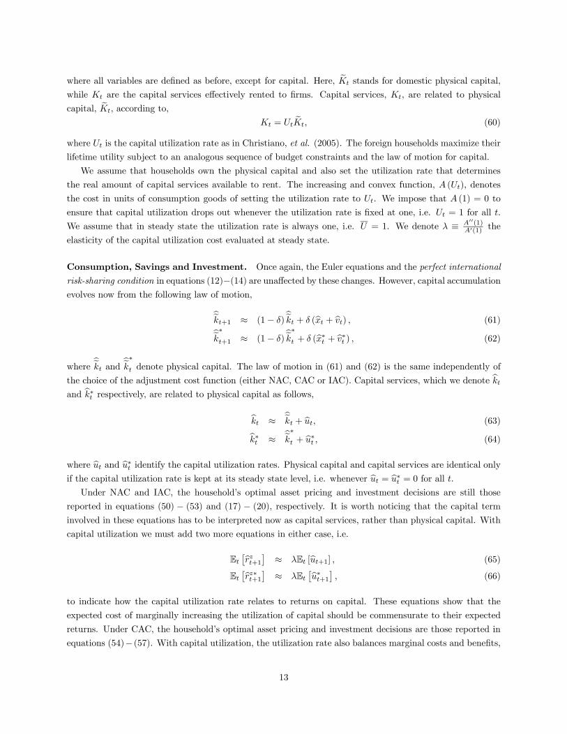
Consumption, Savings and Investment. Once again, the Euler equations and the perfect international

risk-sharing condition in equations (12)−(14) are unaffected by these changes. However, capital accumulationevolves now from the following law of motion,

bekt+1 ≈ (1− δ)bekt + δ (bxt + bvt) , (61)bek∗t+1 ≈ (1− δ)bek∗t + δ (bx∗t + bv∗t ) , (62)

where bekt and bek∗t denote physical capital. The law of motion in (61) and (62) is the same independently ofthe choice of the adjustment cost function (either NAC, CAC or IAC). Capital services, which we denote bktand bk∗t respectively, are related to physical capital as follows,

bkt ≈ bekt + but, (63)bk∗t ≈ bek∗t + bu∗t , (64)

where but and bu∗t identify the capital utilization rates. Physical capital and capital services are identical onlyif the capital utilization rate is kept at its steady state level, i.e. whenever but = bu∗t = 0 for all t.Under NAC and IAC, the household’s optimal asset pricing and investment decisions are still those

reported in equations (50) − (53) and (17) − (20), respectively. It is worth noticing that the capital terminvolved in these equations has to be interpreted now as capital services, rather than physical capital. With

capital utilization we must add two more equations in either case, i.e.

Et£brzt+1¤ ≈ λEt [but+1] , (65)

Et£brz∗t+1¤ ≈ λEt

£bu∗t+1¤ , (66)

to indicate how the capital utilization rate relates to returns on capital. These equations show that the

expected cost of marginally increasing the utilization of capital should be commensurate to their expected

returns. Under CAC, the household’s optimal asset pricing and investment decisions are those reported in

equations (54)− (57). With capital utilization, the utilization rate also balances marginal costs and benefits,

13

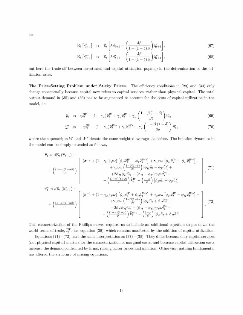
i.e.

Et£brzt+1¤ ≈ Et

∙λbut+1 −µ δβ

1− (1− δ)β

¶ bqt+1¸ , (67)

Et£brz∗t+1¤ ≈ Et

∙λbu∗t+1 −µ δβ

1− (1− δ)β

¶ bq∗t+1¸ , (68)

but here the trade-off between investment and capital utilization pops-up in the determination of the uti-

lization rates.

The Price-Setting Problem under Sticky Prices. The efficiency conditions in (29) and (30) only

change conceptually because capital now refers to capital services, rather than physical capital. The total

output demand in (35) and (36) has to be augmented to account for the costs of capital utilization in the

model, i.e.

byt ≈ ηbtWt + (1− γx)bcWt + γxbxWt + γx

µ1− β (1− δ)

βδ

¶but, (69)

by∗t ≈ −ηbtWt + (1− γx)bcW∗t + γxbxW∗t + γx

µ1− β (1− δ)

βδ

¶ bu∗t , (70)

where the superscripts W and W ∗ denote the same weighted averages as before. The inflation dynamics in

the model can be simply extended as follows,

bπt ≈ βEt (bπt+1)++³(1−α)(1−αβ)

α

´⎡⎢⎢⎢⎢⎢⎣¡σ−1 + (1− γx)ϕω

¢ £φHbcWt + φFbcW∗t

¤+ γxϕω

£φHbxWt + φF bxW∗t

¤+

+γxϕω³1−β(1−δ)

βδ

´[φHbut + φF bu∗t ] +

+2φHφF brst + (φH − φF ) ηϕωbtWt −−³(1−ψ)(1+ϕ)

ψ

´bkWt − ³1+ϕψ ´[φHbat + φFba∗t ]

⎤⎥⎥⎥⎥⎥⎦ ,(71)

bπ∗t ≈ βEt¡bπ∗t+1¢+

+³(1−α)(1−αβ)

α

´⎡⎢⎢⎢⎢⎢⎣¡σ−1 + (1− γx)ϕω

¢ £φFbcWt + φHbcW∗t

¤+ γxϕω

£φF bxWt + φHbxW∗t

¤+

+γxϕω³1−β(1−δ)

βδ

´[φF but + φHbu∗t ]−

−2φFφH brst − (φH − φF ) ηϕωbtWt −−³(1−ψ)(1+ϕ)

ψ

´bkW∗t −³1+ϕψ

´[φFbat + φHba∗t ]

⎤⎥⎥⎥⎥⎥⎦ .(72)

This characterization of the Phillips curves requires us to include an additional equation to pin down the

world terms of trade, btWt , i.e. equation (39), which remains unaffected by the addition of capital utilization.Equations (71)−(72) have the same interpretation as (37)−(38). They differ because only capital services

(not physical capital) matters for the characterization of marginal costs, and because capital utilization costs

increase the demand confronted by firms, raising factor prices and inflation. Otherwise, nothing fundamental

has altered the structure of pricing equations.

14

3 Model Calibration

In this section, we describe the choice of the parameter values. Our calibration is summarized in Table 1.

For comparison purposes, the parameterization of CKM (2002) and Steinsson (2008) also appears in Table

1. In order to keep our model comparable, our choice of values for the structural parameters is very similar

to theirs.

[Insert Table 1 about here]

We assume that the discount factor, β, equals 0.99 which is consistent with an annual real return of 4%.

We set the intertemporal elasticity of substitution, σ, to 1/5 as in CKM (2002) and Steinsson (2008). The

inverse of the Frisch elasticity of labor supply, ϕ, is set to 3 which is compatible with the available micro

evidence (see, e.g., Browning, et al., 1999, and Blundell and MaCurdy, 1999). This choice also brings the

‘strategic complementarity of consumption’ in the Phillips curve, σ−1 + (1− γx)ϕω, closer to Steinsson’s

(2008) number.

The elasticity of substitution across varieties, θ, is set to 10. This is consistent with a price mark-up of

11% as documented in the U.S. data by Basu (1996).9 Steinsson (2008) sets the intratemporal elasticity of

substitution, η, also equal to 10. We believe this value is rather high in comparison with the usual calibrations

in the international business cycle literature. For instance, Backus, et al. (1995) assume values between 0.9

and 2, while CKM (2002) select 1.5 for their sticky-price model. Empirical work by Lai and Trefler (2002)

finds estimates somewhere in the middle, around 5.5. Our benchmark calibration sets this parameter to 1.5

as in CKM (2002). Obviously, a great deal of uncertainty about the true value still exists.

The home and foreign shares, φH and φF , are set respectively to 0.94 and 0.06. CKM (2002) relies

on these values to match the observation that U.S. imports from Europe are roughly 1.6% of GDP. Our

parameterization is taken directly from theirs. As is conventional, we set the labor share, ψ, equal to 2/3

and the depreciation rate, δ, equal to 0.021. The latter implies an annual depreciation rate of 10% which

is typical for the U.S. data. The Calvo price stickiness parameter, α, is assumed to be 0.75. This implies

that the average price duration in our model is 4 quarters, making it comparable with the degree of nominal

price stickiness assumed in CKM (2002).

The parameterization of the monetary policy rule is identical to Steinsson (2008), except that our rule

targets output rather than consumption. The interest rate inertia parameter, ρi, equals 0.85, while the

weight on the inflation target, ψπ, equals 2, and the weight on the output target, ψy, is 0.5.

The Calibration of Shocks and Other Cost Parameters. We assume identical AR (1) exogenous

processes for the monetary, the real, and the investment-specific shocks and set the persistence of all those

shocks, ρm, ρa and ρv, equal to 0.9. This is in line with the parameterization of Steinsson (2008). In

CKM (2002), the volatility of the monetary innovations is selected to match the volatility of output, and

the correlation of domestic and foreign monetary innovations is calibrated to match the observed cross-

correlation of output. We adopt a similar calibration strategy and set the standard deviation of all shocks9Up to a first-order approximation, the elasticity of substitution across varieties only enters our considerations because the

mark-up affects the steady state investment share (over GDP), γx. The choice of θ equal to 10 as a free parameter impliesthat the steady state investment share is 0.203. In Cooley and Prescott (1995), after excluding both the stock of governmentcapital and the income that it generates, the investment share is calculated at 0.252. Hence, our choice of the parameter θ isboth consistent with empirical estimates of the mark-up and with the long-run measures of the investment share.

15

to match the output volatility in the U.S. data (i.e., 1.54%). In addition, we calibrate the cross-country

correlation of all innovations to replicate the observed cross-correlation of U.S. and Euro-zone GDP (i.e.,

0.44).

In the exercise where both monetary and real shocks drive the business cycle, we assume that real shock

innovations are 4 times as volatile as monetary innovations. This is based on the results in Søndergaard

(2004) who infers the volatility of U.S. real and monetary innovations from estimates of productivity and

a Taylor rule for the U.S. We assume that the cross-country correlation of real innovations is identical to

that of monetary innovations. Given these constraints, we calibrate the volatility and correlation of real

innovations to match the volatility and cross-country correlation of GDP in the data.

Finally, we select the appropriate capital or investment adjustment cost parameter, either χ or κ, to

ensure that investment volatility in the model is as volatile as in the data (i.e., 3.38 times as volatile as U.S.

GDP in real terms)10 . In models with capacity utilization, we set the elasticity of capital utilization costs,

λ, to match the value of 5.80 estimated by Justiniano, et al. (2008).

4 Quantitative Findings11

In this section, we examine how adding capital accumulation affects the performance of our open economy

model, and ask whether a sticky-price model with pricing-to-market can generate the type of international

business cycle fluctuations that can be observed in the data between the U.S. and the Euro-zone. To answer

this question, we compare a model set-up with capital and investment adjustment costs (IAC) against an

alternative model with linear-in-labor technologies and no capital (NoC). In Table 2, we analyze the effects

of monetary shocks over the business cycle. In Tables 3, 4 and 5 we explore respectively the contribution of

real shocks, investment-specific shocks and a combination of monetary and real shocks.

While our primary focus is how the model explains real exchange rate dynamics, we also report a number

of relevant business cycle moments for each simulation. In particular, we make an extra effort to cross-validate

the main predictions of our model by showing whether or not getting the real exchange rate right comes

at the expense of worsening the model predictions along some other dimension of interest. Of particular

importance, obviously, is monitoring the impact the model has on trading patterns.

We also test the robustness of our conclusions to the specification of different adjustment cost functions

(see, e.g., CKM, 2002) and to the assumption of variable capital utilization rates (see, e.g., Christiano, et

al., 2005).

The Features of the Data. The main features of the data are well-known from the work of CKM (2002).

Real U.S. GDP has a standard deviation of 1.54%, while U.S. investment and consumption are respectively

3.38 and 0.81 times as volatile as GDP. All three series are very persistent with a first-order autocorrelation

around 0.85. In the data, the cross-country correlation of U.S. GDP with Euro-zone GDP is higher, at 0.44,

10We use the adjustment cost parameter to match the volatility of investment instead of the volatility of consumption asin CKM (2002). Thus, in our case, the volatility of consumption is endogenously determined (rather than chosen). This hasimplications for the volatility of the real exchange rate, which in turn makes the simulations easier to interpret: If the modeldoes not generate enough consumption volatility, it is likely not to deliver the right real exchange rate volatility.

11All our simulation results have been generated using the software package Dynare (see, e.g., Juillard, 2003), while thetheoretical moments are all based on Hodrick-Prescott filtered time-series.

16

than either consumption or investment, both at 0.33. U.S. employment relative to GDP, in turn, is less

volatile at 1.02%, less correlated across countries at 0.29, but more persistent at 0.92.

One of the central puzzles in international business cycles, the PPP puzzle, arises empirically because

the real exchange rate is known to be quite volatile and persistent. The standard deviation of the real

exchange rate is about 5.14 times that of U.S. GDP12, and its first-order autocorrelation is close to 0.78.

These moments, however, are notably hard to derive in an endogenous open-economy model, even under

price-stickiness and pricing-to-market. Hence, this gives rise to the PPP puzzle.

Finally, the real exchange rate is expected to play a significant role in determining cross-country trade

patterns, since international relative prices determine the size of the expenditure-switching effect. With

regards to trade, we note that the real trade balance is barely 0.25 times more volatile than GDP, but real

exports and imports are respectively 2.59 and 3.31 times more volatile. All export-related series are very

persistent, around 0.83− 0.85. But U.S. exports and imports tend to display some differences; for instance,U.S. GDP is positively correlated with U.S. exports and imports, but the correlation with imports is twice

as strong (0.82 versus 0.41). U.S. GDP is also negatively correlated with net exports at −0.47, while exportsand imports are positively correlated at a low value of 0.21. For more details on the observed trade patterns,

see also Engel and Wang (2007) and Raffo (2008a).

Is Perfect International Risk-Sharing Incompatible with the Data? A general equilibrium model

with complete international financial markets implies a fairly tight link between real exchange rates and

relative consumption. As argued by CKM (2002), the perfect international risk-sharing condition in (14) gives

rise to the Backus-Smith puzzle; that is a theoretical high positive correlation between relative consumption

and the real exchange which is not consistent with the data (see Backus and Smith, 1993). The question

is whether this tight link between relative prices and quantities hinders our ability to simultaneously match

the volatility and persistence of output, consumption and the real exchange rate.

Given the household preferences, the connection between real exchange rate and consumption volatility

can be expressed as,var ( brs)var (by) ∼= 2

σ2[1− corr (bc,bc∗)] var (bc)

var (by) . (73)

Similarly, the real exchange rate persistence implied by the model is tied to the persistence of consumption

such that the first-order autocorrelations of both are approximately equal, i.e.

corr ( brs, brs−1) ∼= corr (bc,bc−1) . (74)

Hence, our model’s ability to generate real exchange rate volatility hinges on whether it can generate sufficient

consumption volatility and the right consumption cross-correlation; while the persistence of the real exchange

rate and the persistence of consumption are like two-sides of the same coin.13

As a starting point, we ask ourselves to what extent the perfect international risk-sharing condition, as

12Our measure of RER volatility is comparable to that used by CKM (2002). Our raw measure of RER volatility is 7.94%compared to 7.91% in CKM (2002). Our GDP is slightly less volatile than CKM (2002) (1.54% vs. 1.82%). The main reasonfor the discrepancy in the ratio is that our sample period captures more of the Great Moderation era than theirs does. Theimplication is that relative to GDP, the volatility of the RER is 4.36 in CKM (2002) and 5.14 in our dataset. We believe thenumber is nonetheless relevant for the purpose of this paper.

13For more details on the derivation of equations (73) and (74), see the Appendix.

17

it transpires in (73) and (74), is compatible with the data itself. First, we observe that the consumption

first-order autocorrelation in the data is 0.87 compared with 0.78 for the real exchange rate. Second, we find

that the empirical cross-country correlation of consumption and the empirical volatilities of consumption and

GDP imply a model-consistent volatility for the real exchange rate relative to GDP of 4.40, compared with

5.14 in the data.14 Given our choice of preferences, and particularly our parameterization of the elasticity

of substitution, perfect international risk-sharing is not outright inconsistent with the features of either

consumption or the real exchange rate as observed in the data. Furthermore, we can say that if our theory

is unable to match the properties of either consumption or the real exchange rate, it likely fails to match

them both.

4.1 Monetary Policy Shocks

The first set of our experiments assumes that all exogenous disturbances are monetary policy shocks. To

shed light on the relationship between capital accumulation and real exchange rate dynamics, we compare

simulation results from a model with capital accumulation (IAC) with results from a model with no capital

(NoC).

4.1.1 Impulse Responses

Figure 1 shows the impulse responses for a contractionary domestic monetary policy shock (i.e., an increase inbεmt ) in our benchmark model with capital (IAC) as well as our model without capital (NoC). The qualitativeeffects of a monetary contraction are similar in the two models. Higher interest rates increase the cost of

consuming today relative to saving for tomorrow.15 Domestic consumption and, hence, aggregate demand

falls in both models.

[Insert Figure 1 about here]

How do monetary shocks affect the real exchange rate? The impulse responses in Figure 1 indicate that

a contractionary monetary shock causes the domestic currency to appreciate in real terms. The intuition

follows naturally from the perfect international risk-sharing condition in (14) which links the real exchange

rate to domestic and foreign consumption.

Since the domestic and foreign monetary shocks are assumed to be correlated (in order to match the

cross-country correlation of GDP), foreign consumption declines as well. Given that the monetary policy

shock originates in the domestic economy, it triggers a greater decline in domestic consumption, bct, thanin foreign consumption, bc∗t . Hence, consumption becomes relatively higher in the foreign country, and theinternational risk-sharing condition implies that the real exchange rate, brst, has to fall becoming relatively‘cheaper’ (i.e., a real appreciation from the domestic point of view).

While the qualitative results are identical in models with and without capital, there are important

quantitative differences.16 Figure 1 shows that the required real exchange rate appreciation is relatively14To exactly match the real exchange rate volatility in the data we would need to reduce the elasticity of substitution from

15to 1

5.84.

15However, without price stickiness, all monetary policy shocks would translate into inflation and have no impact on realinterest rates.

16While the shape of most impulse response functions is very similar for the models with and without capital, there aresignificative differences on the trade patterns. Most notably, on the dynamics of domestic imports.

18

smaller in our benchmark with capital. In this case, a contractionary monetary policy shock increases the

cost of consuming today relative to saving for tomorrow through the Euler equations in (12) and (13), and

households choose to postpone consumption today. It also increases the cost of capital through the asset

pricing equations for Tobin’s q in (54) and (56), lowering the investment demand.17 The greater volatility

of investment and the attenuated spill-overs into the foreign economy ultimately forces relative prices (in

particular, the real exchange rate) to play a greater role to help switch expenditure across country and

equate the domestic supply to the sum of domestic and foreign demand.

Alternatively, one could simply argue that without access to physical capital, households cannot smooth

consumption by dissaving in the immediate periods following a contractionary monetary policy shock. There

is no intertemporal channel for them to transfer production from one period to the next. Therefore, their

consumption has to fall by a larger amount relative to a set-up where they could alter their investment-savings

decisions in response to that shock.

The impulse responses illustrate the persistence problem inherent in both models. The real exchange rate

responds sharply in period 1 but then reverts fairly rapidly towards its steady state. From period 4 onwards,

the real exchange rate dynamics are quite muted. The response of the real exchange rate to a monetary

shock is not hump-shaped either, because output and inflation move in the same direction (contrary to

what happens in response to a real shock) and monetary policy does not have to balance out two conflictive

objectives (see, e.g., Steinsson, 2008).18 But it becomes slightly more gradual without capital, which explains

why the NoC model gets a little bit more persistence than our benchmark out of a monetary shock.

4.1.2 Theoretical Moments

Other features of the business cycle, particularly consumption, output and investment, are as important as

the real exchange rate. We realize that real exchange rates, as relative prices, influence the expenditure-

switching across countries and hence the trade flows. So, we pay special attention to the implications

of capital for the model’s ability to replicate observed fluctuations in export and import volumes. The

performance of each model is assessed by comparing the theoretical moments with the empirical business

cycle statistics for the main variables of interest.

The theoretical moments from simulating our benchmark economy in response to monetary shocks are

summarized in the second column of Table 2, under the header ‘IAC’. For easy comparison, the third column

contains the simulation results for a model with no capital accumulation, under the header of ‘NoC’.

[Insert Table 2 about here]

One key result from Table 2 is that the model without capital (NoC) generates real exchange rates that

are more volatile than what we observe in the data. The volatility of real exchange rates relative to output

implied by this particular model is 6.44 times the volatility of output, while in the data is just 5.14 times

more volatile. However, the model without capital fails to produce a sufficiently persistent real exchange

17CKM (2000) point out that investment is particularly interest-sensitive in a closed economy sticky-price model written inthe same spirit as ours. Our results confirm that this is also true in an open economy framework.

18The simulation results for CPI inflation and nominal interest rates are not reported but can be obtained directly from theauthors upon request.

19

rate, since the theoretical autocorrelation of the real exchange rate is 0.52 against 0.78 in the data. Not

surprisingly, by the approximation in (74), consumption appears also much less persistent than in the data,

0.50 versus 0.87.

In contrast, the benchmark model with capital (IAC) produces real exchange rates that are both less

volatile at 5.13 times the volatility of output, and less persistent at 0.44. So while both types of models

appear to resolve the international pricing puzzle, they fail to account for the persistence anomaly. These

findings are broadly in line with CKM (2002) and Steinsson (2008)19 . What makes the low persistence all

the more puzzling is that, unlike CKM (2002), we rely on very persistent monetary shocks in an attempt

to give them a better chance to match the persistence of the real exchange rate, and we also introduce

further persistence through the investment equations in (18) and (20). But that is not enough to raise the

autocorrelation.

The business cycle statistics for consumption illustrates why the model without capital (NoC) generates

more real exchange rate volatility than our benchmark model (IAC). Consumption in the benchmark case

is both less volatile and less persistent, with a volatility of 0.81 and an autocorrelation of 0.44, relative

to the set-up with no capital, with a volatility of 1.07 and an autocorrelation of 0.52. The cross-country

correlation of consumption is also lower in the benchmark with capital, 0.20 versus 0.2820. These facts, and

the mechanics of volatility described in (73), explain how the model still manages to generate a very volatile

real exchange rate.

Another significant insight from Table 2 is that the benchmark model (IAC) appears to perform remark-

ably well in terms of matching key international business cycle statistics. The volatility of consumption, net

exports and real exports and imports is roughly in line with the data. The benchmark is able to reproduce

some of the trademark differences between exports and imports. For instance, it produces a lower correlation

between domestic output and exports than between domestic output and imports, 0.20 and 0.62 respectively.

It produces more volatility for imports than exports, although it often understates the magnitude of the ex-

ports volatility and induces a negative correlation between exports and imports21. All these features are

otherwise hard to replicate in a model with flexible prices and no home bias (see, e.g., Engel and Wang,

200722).

19 Steinsson (2008) develops two main variants of his model without capital: the homogenous labor market model, and theheterogenous market model. The difference between the two variants is in the degree of ‘strategic complementarity’ in thePhillips curve. In other words, the slope of the Phillips curve is flatter under heterogenous labor markets. Steinsson (2008)shows that heterogenous labor markets induce higher persistence in response to a monetary shock, although still below the data,at the expense of lower real exchange rate volatility relative to consumption. However, it does not show whether consumptionvolatility varies between specifications. The underlying assumption in our model is that labor markets are competitive andlabor itself is an homogeneous production factor. Hence, our model is comparable to Steinsson’s (2008) homogenous labormarket model.

20The elasticity of intertemporal substitution might be a little bit higher than what is needed to reconcile the volatilities ofconsumption and the real exchange rate with the cross-correlation of consumption. Hence, even though the IAC model matchesthe volatility of consumption and the real exchange rate, it generates less consumption cross-correlation than the data (0.20versus 0.33).

21Our sensitivity analysis also involved examing the role played by the home bias parameter. We tried an alternative modelset-up where we re-calibrated the home bias parameters (simultaneously with the adjustment cost parameter, and the volatilityand the correlation of shock innovations) to match the volatility of real imports and real exports in response to a monetaryshock. In the IAC specification this requires us to set φF = 0.22, instead of using the value of 0.06 in our benchmark calibration.

22However, we also find that sticky prices and home bias in consumption and investment help account for differences in thebusiness cycle features of exports and imports.

20

The model also implies a correlation between net exports and GDP of −0.45, similar to the empiricalcorrelation of −0.47. The autocorrelation statistics illustrate that the benchmark model (IAC) as well asthe model with no capital (NoC) do not create enough persistence, and not only on consumption and real

exchange rates. For example, the theoretical autocorrelation of GDP is 0.62, which is less than the 0.87

observed in the data.

The failure of sticky-price models to generate endogenous persistence from monetary policy shocks has

been pointed out in a closed economy setting by CKM (2000) and in an open economy setting by CKM

(2002). The results in Table 2 suggests that neither the benchmark model nor the model without capital

can resolve the persistence anomaly.

4.1.3 Specification Robustness

This section examines the sensitivity of our results to alternative specifications of the adjustment cost

functions. The investment adjustment cost (IAC) case adopted as our benchmark makes capital adjustment

more ‘costly’ relative to the more conventional capital adjustment cost (CAC) function used by CKM (2002).

With IAC costs, households are penalized for altering the growth rate of investment (see equations (55) and

(57)) unlike CAC costs where it is costly to alter the investment-to-capital ratio (see equations (18) and

(20)). For completeness, we also consider the case of no capital adjustment costs (NAC).

The simulation results from the two additional experiments are summarized in Table 2, columns 4 and

5 respectively, under the headers ‘CAC’ and ‘NAC’. The key insight from these experiments is that the real

exchange rate dynamics generated by the model depend crucially on whether adjustment costs are added to

the law of motion for capital or not. Without adjustment costs (NAC), the model implies a very volatile

investment series, 5.08 times as volatile as output versus 3.38 times in the data. Households smooth their

consumption in response to monetary shocks by adjusting their capital stock freely. Not surprisingly, the

NAC case generates a very smooth consumption series, where the volatility of consumption equals 0.03. The

low volatility of consumption, in turn, translates into very little real exchange rate volatility (only 0.19 times

the volatility of output).

This model setup also generates very low persistence in GDP, investment and employment but, actually,

high persistence in consumption and the real exchange rate. The consumption and real exchange rate

autocorrelations are in the neighborhood of 0.78, surprisingly close to their empirical counterparts.

Another key insight is that the functional form of the adjustment cost function also does matter. The

CKM-type adjustment costs (CAC) imply a ratio of consumption to GDP volatility of 0.49. Relative to

the benchmark case (IAC), the CAC model generates only half the consumption volatility. Our intuition is

that relative to the IAC case, now it is less costly to change the level of investment. Households can more

easily smooth consumption by adjusting their investment margin much more on impact. Since the cross-

correlation of consumption is quite similar in the IAC and CAC models, this lower volatility of consumption

mechanically translates into lower real exchange rate volatility relative to the IAC benchmark (only 3.09

times the volatility of output versus 5.13 in the IAC case).

But in terms of real exchange rate persistence, the CAC model does not differ markedly from our bench-

mark. They both generate insufficiently low theoretical autocorrelations in the neighborhood of 0.44− 0.45.

21

4.2 Real Shocks

The second set of our experiments assumes that all exogenous disturbances are real shocks. The motivation

for carrying out this exercise is twofold: First, the international real business cycle literature has always

emphasized the importance of real shocks driving the business cycle. Second, Steinsson (2008) has shown

that a model with real shocks (albeit one without capital) has the ability to match the empirical persistence

and volatility of the real exchange rates. To shed light on the relationship between capital accumulation and

real exchange rate dynamics, we compare simulation results from a model with capital accumulation (IAC)

with results from a model with no capital (NoC).

4.2.1 Impulse Responses

Figure 2 shows impulse response functions for a positive domestic real shock (i.e., an increase in bεat ) inthe two models (IAC) and (NoC). Higher productivity increases output on impact, lowers employment,

brings real marginal costs down and, therefore, tends to lower CPI inflation.23 All of this creates conflicting

objectives for monetary policy, because output and inflation move in opposite directions. The higher output

in the domestic economy creates a larger worldwide supply of domestic goods. To clear the goods market,

either domestic aggregate demand (i.e., consumption and investment) has to rise and/or net exports has to

increase.

In the benchmark case with capital (IAC), the adjustment mainly comes about via a large rise in domestic

investment and a small increase in both net exports and domestic consumption. In the model with no capital

(NoC), demand and supply equate through a large rise in both domestic consumption and net exports. This

in turn requires a larger movement in relative prices for the external sector to adjust and, in particular,

a larger rise in the real exchange rate (a real domestic depreciation) than what is needed in a model with

capital.

The impulse responses illustrate that the real shock triggers a hump-shaped response in consumption and

the real exchange rate for both the models with and without capital. This hump-shaped impulse responses

arise because of the conflicting monetary policy objectives between output and inflation, as discussed in

Steinsson (2008).24 In addition, Figure 2 confirms that the magnitude of the response is much greater in the

model without capital. At its peak around the fourth quarter, the real exchange increases by almost 50%

more in the model without capital.

[Insert Figure 2 about here]

Summing up, households have more difficulty smoothing consumption without access to physical capital

(the intertemporal channel). Hence, the perfect international risk-sharing condition in (14) implies a greater

real exchange rate depreciation since consumption increases by more (and becomes more volatile) in a model

without capital.23The results of the simulation for CPI inflation and nominal interest rates are discussed in the paper, but not always reported.

They can be obtained directly from the authors upon request.

24The deflationary effects from the positive real shock causes the domestic monetary authorities to lower domestic nominalinterest rates to balance their conflicting policy objectives, and to lead real interest rates into negative territory over time.For a while, this reinforces the tendency to consume more and save less, and induce more investment through the investmentequations. This subsequent rise in consumption and investment boosts demand, hence triggering the hump-shaped response ofconsumption and real exchange rates.

22

What appears to be more surprising is that domestic imports tend to stabilize quickly in the benchmark

model with capital (IAC), while they take a big dip in the model without capital (NoC). Because of the

import content in investment, any rise in investment requires a rise in imports. This additional demand

partly offsets the decline in imports stemming from the expenditure-switching effect induced by the real

exchange rate. In other words, it appears that for our calibration the ‘income effect’ quickly overtakes the

‘relative price effect’ specifically on imports. The importance of investment goods in trade has also been

argued recently by Engel and Wang (2007).

4.2.2 Theoretical Moments

The results for the benchmark case are reported in Table 3, column 2, under the header ‘IAC’. The case

with no capital can be found in column 3, under the header ‘NoC’. For the benchmark case (IAC), the real

exchange rate is around 1.64 times as volatile as output, while in the data the real exchange rate is 5.14

times more volatile than GDP. Hence, it does not appear that a model with capital and real shocks can

resolve the international pricing puzzle. However, the model with capital generates a sufficiently persistent

real exchange rate since the theoretical autocorrelation of 0.84 even exceeds the 0.78 observed in the data.

In contrast, a model with no capital (NoC) generates roughly twice the real exchange rate volatility

as the benchmark model, that is 3.14 times the volatility of output. Real exchange rates are also highly

persistent with an autocorrelation of 0.85 in the model without capital. Both findings are consistent with

the evidence presented by Steinsson (2008). While neither model can rely on real shocks alone to generate

enough real exchange rate volatility, real shocks do help account for the persistence anomaly and eliminating

capital tends to amplify their effect on the volatility of the real exchange rate.

[Insert Table 3 about here]

As with monetary shocks, the investment (intertemporal) channel plays a critical role here. Without

access to physical capital, households have more difficulty smoothing consumption. So consumption and the

real exchange rate become more volatile in the NoC case, by the mechanics at play in (73). In the benchmark

with capital (IAC), consumption is too smooth relative to the data (0.39 times as volatile as output versus

0.81 times in the data). However, consumption, investment and output exhibit a high degree of persistence

that comes close to matching their empirical counterparts.

Turning now to other business cycle moments, the model with capital (IAC) generates a cross-country

correlation of consumption at 0.65 that is considerably higher than in the data, where it stands at only

0.33. The cross-country correlation of GDP at 0.44 is matched by construction, but then consumption

endogenously becomes more correlated than GDP unlike what we observe in the data. In the model without

capital (NoC), consumption is more than twice as volatile as in the IAC case (0.91 times the volatility of

output versus 0.39 times). Also the consumption cross-correlation is 0.76 in the NoC, which is higher than

the 0.65 reported in the IAC case. However, the increase in the volatility of consumption suffices to almost

double the real exchange rate volatility that the model without capital (NoC) can get from a domestic real

shock.

In summary, while real shocks can generate sufficiently persistent real exchange rates in a model with

capital (IAC) and a model without capital, the lower volatility of consumption in the model with capital

(and the high consumption cross-correlation) can only be consistent with a lower real exchange rate volatility

23

under perfect international risk-sharing. Hence, models with capital have more difficulty resolving the PPP

puzzle relative to models without capital such as Steinsson’s (2008).

4.2.3 Specification Robustness

This section examines how the model properties change when alternative adjustment functions are being

considered in place of the IAC. The simulation results for the CKM-style adjustment costs are summarized in

Table 3, column 4, under the header ‘CAC’. The case of no adjustment costs appears in column 5, under the

header ‘NAC’. The interpretation of the results is similar to the one given for the experiment with monetary

shocks. The less costly it is to alter the capital stock, the greater the ability for households to smooth their

consumption.

As a result, consumption is very smooth in the NAC case and less so in the CAC case (0.15 times and

0.35 times as volatile as output, respectively). The smooth consumption series translates into real exchange

rates that are not very volatile (only 0.56 times as volatile as output in the NAC case and 1.51 times as

volatile in the CAC setup). Interestingly, while the functional form of adjustment costs played a large role in

the case of monetary shocks, the simulation results suggest that for real shocks there are no large differences

between the CAC and the IAC specifications. In fact, the volatility and persistence of all variables is roughly

similar in both cases.

5 Sensitivity Analysis

This section examines the sensitivity of our results to model variations that have been either explored or

proposed elsewhere in the literature.

5.1 Investment-Specific Shocks

Christiano, et al. (2005) and Justiniano and Primiceri (2008) have recently pointed out that investment-

specific shocks can be a key driver for the business cycle, while Raffo (2008b) has argued that these shocks

are important to help us understand terms of trade. Hence, an unavoidable question is can these shocks also

resolve the PPP puzzle?

We have therefore re-simulated our benchmark model (IAC) assuming that investment-specific shocks

are the only exogenous disturbances. Table 4, column 2, contains the results for the benchmark. For

completeness, we have also examined the role of these shocks in combination with capital adjustment costs

(CAC) and with no adjustment costs (NAC). The simulation results from these experiments are summarized

in Table 4, column 4 and 5.

[Insert Table 4 about here]

The general message from Table 4 is that investment-specific shocks are not likely to be the most relevant

force to induce data-comparable dynamics for the real exchange rate within an open-economy, sticky price

model. While the IAC model does a good job at matching employment volatility (it becomes 0.64 times

as volatile as output against 0.66 in the data), consumption is too smooth (only 0.39 times as volatile as

output). Moreover, there is too much consumption cross-correlation across countries (0.65 versus 0.33 in the

24

data) and as a result the real exchange rate is not volatile enough. The volatility of the real exchange rate

is only 1.63 times that of output instead of 5.14 times as in the data.

However, investment-specific shocks combined with capital adjustment costs do imply a very persistent

real exchange rate series. The autocorrelation of the real exchange rate is 0.96 in the benchmark case

(IAC), and 0.93 in the CAC setup. Figure 3 plots the impulse response functions for a positive domestic

investment-specific shock.

[Insert Figure 3 about here]

While these shocks are temporary in nature, they appear to trigger model dynamics that take a very

long time to propagate its way through the system. For instance, domestic investment only appears to peak

12 − 14 quarters following an investment-specific shock. In contrast, as Figures 1 and 2 show, domesticinvestment peaks 4 quarters after a monetary shock and 8 quarters after a real shock. So investment-specific

shocks have the potential to generate lots of persistence, but cannot resolve the international pricing puzzle.

5.2 Capital Utilization

Christiano, et al. (2005) have shown in a closed-economy framework how variable capital utilization can help

generate persistent output effects following a monetary shock. It seems a natural question to ask whether

adding capital utilization in the same spirit as Christiano, et al. (2005) can generate volatile and persistent

real exchange rates in an open-economy, sticky-price model. We re-simulate the IAC model, the CAC model

and the NAC model for each one of the 3 different types of shocks (real, monetary and investment-specific)

to provide an answer to that. The simulation results are summarized in the final 3 columns in Tables 2, 3

and 4.

The most interesting results are for the case of monetary shocks in Table 2, columns 6 to 8. The

benchmark case with capital utilization (under the header ‘IAC+CU’) only produces consumption volatility

of 0.44 times that of output, and real exchange rate volatility of 2.65 times that of output. Contrast this with

the benchmark case without capital utilization (IAC), where consumption and real exchange rate volatility

relative to output is 0.81 times and 5.13 times respectively. At the same time, the real exchange rate

persistence with capital utilization decreases to merely 0.38 versus 0.44 in the benchmark IAC case.

It appears that adding capital utilization impedes or hampers the model’s ability to resolve the PPP

puzzle. Our intuition is that capital utilization offers a way, albeit a costly one, to get around the adjustment

constraints on investment. In other words, capital utilization allows households to make better use of the

intertemporal smoothing channel. Hence, resulting in lower consumption and real exchange rate volatilities.

Adding capital utilization to a model featuring the alternative capital adjustment function (CAC) yields a

similar conclusion.

5.3 Real and Monetary Shocks

Up to this point, our simulations have assumed that international business cycles are either driven by

monetary shocks, by real shocks or by investment-specific shocks alone. Here, instead, we explore the case

where our open economy model is subject to both exogenous monetary and real disturbances. The results

for the benchmark case (IAC) are summarized in Table 5, column 2. Column 3 contains results for the model

without capital (NoC).

25

[Insert Table 5 about here]

The main observation from Table 5 is that the benchmark IAC model, when simulated with both real and

monetary shocks, produces real exchange rates that are 3.12 times more volatile than GDP. While this value

is less than what we observe in the data, where we find that the real exchange rate is 5.14 times as volatile

as GDP, the benchmark now produces twice as much real exchange rate volatility as was the case with just

real shocks. The model without capital (NoC) is, once again, capable of almost perfectly replicating the

empirically observed real exchange rate volatility, 5.23 times versus 5.14 times the volatility of GDP in the

data. So our main message remains robust, namely that models without capital suffer from a ‘volatility bias’

that tends to understate the true magnitude of the international pricing puzzle.

Interestingly, the benchmark IAC model with both types of shocks implies a real exchange rate persistence

that is only slightly higher than the autocorrelation we compute with just monetary shocks. Here, the

autocorrelation of the real exchange rate is 0.50, while it is 0.44 in the case of monetary shocks only. Why

is this finding important? Our earlier analysis has somewhat validated the results of Steinsson (2008) that

real shocks have the potential to resolve the persistence anomaly of real exchange rates, albeit in a model

without capital. However, Table 5 illustrates that when monetary shocks are added as one (although not

the exclusive) source of business cycle fluctuations, the theoretical autocorrelation of the real exchange rate

drops significatively to 0.50.

Therefore it appears that in this class of open-economy, sticky-price models, even if real shocks are the

dominant source on business cycle fluctuations for most macro aggregates, the real exchange rate dynamics

are still disproportionately impacted by the monetary shocks.

[Insert Table 6 about here]

This is confirmed by Table 6 which contains a variance decomposition for the benchmark model. Each

column indicates the fraction of variance coming from the 4 shocks (domestic and foreign monetary policy

and productivity shocks) in the benchmark IAC model. We note that almost 80% of all the variability in

the real exchange rate can be attributed to monetary policy shocks. So even though our model calibration

assumes that real shocks are 4 times as volatile as monetary shocks, real exchange rate dynamics including

the volatility and persistence are still tied down mostly by the effects and propagation of the monetary

shocks.25

6 Concluding Remarks

In this paper, we use an open-economy, sticky-price model with pricing-to-market and complete asset markets

to examine the link between real exchange rate dynamics and what the model assumes about physical capital.

We show that this class of models without capital accumulation tend to suffer from a ‘volatility bias’; that

is, they often understate the true magnitude of the international pricing puzzle. In a world without capital,

households cannot smooth consumption easily and rely more heavily on (intratemporal) international trading

in the goods markets for risk-sharing purposes. As a result, consumption and, hence, real exchange rates are

25We would speculate that the disproportionate importance of monetary shocks may be due to the fact that the degree of‘complementarity on consumption’ (in the Phillips curve) is pretty high in our specification, which makes the inflation dynamicsparticularly susceptible to monetary shocks.

26

more volatile relative to models that feature capital accumulation. Our results suggest that resolving the

international pricing puzzle remains challenging once capital is included.

By their very own nature, adjustment costs make it more costly to smooth consumption through the

intertemporal margin. Hence, consumption becomes more volatile and so does the real exchange rate. In

fact, we show that such a model combined with monetary policy shocks has the potential to replicate the

observed real exchange rate volatility. But, when we assume more realistically that business cycles are partly

(if not predominantly) driven by real shocks, the same model produces real exchange rates that are far less

volatile than in the data.

Addressing the CKM (2002) persistence anomaly is not easy either. This paper shows that the anomaly

in response to monetary shocks is robust to adding capital or not, to the specification of the adjustment

costs in the law of motion for capital, and even to the addition of capital utilization. Persistence is easier to

get from real or investment-specific shocks, but then it is rather difficult to match the volatility of the real

exchange rate for a sensible calibration. In our view, the PPP puzzle is still very much alive and well.

27

References[1] Backus, David K. and Gregor W. Smith (1993): "Consumption and Real Exchange Rates in Dynamic

Economies with Non-Traded Goods". Journal of International Economics, vol. 35 (3-4), pp. 297-316.

[2] Backus, David K., Patrick J. Kehoe and Finn E. Kydland (1995): "International Business Cycles:Theory and Evidence", in Thomas F. Cooley (ed.) Frontiers of Business Cycle Research, pp. 331-356.Princeton University Press: Princeton, New Jersey, USA.

[3] Basu, Susanto (1996): "Procyclical Productivity: Increasing Returns or Cyclical Utilization?". Quar-terly Journal of Economics, vol. 111 (3), pp. 719-751.

[4] Benigno, Gianluca (2004): "Real Exchange Rate Persistence and Monetary Policy Rules". Journal ofMonetary Economics, vol. 51 (3), pp. 473-502.

[5] Bergin, Paul R. and Robert C. Feenstra (2001): "Pricing-to-Market, Staggered Contracts, and RealExchange Rate Persistence". Journal of International Economics, vol. 54 (2), pp. 333-359.

[6] Blanchard, Olivier J. and Charles M. Kahn (1980): "The Solution of Linear Difference Models UnderRational Expectations". Econometrica, vol. 48 (5), pp. 1305-1311.

[7] Blundell, Richard and Thomas MaCurdy (1999): "Labor Supply: A Review of Alternative Approaches",in O. Ashenfelter and D. Card (eds.) Handbook of Labor Economics, vol. 3, pp. 1559-1665. ElsevierScience B.V., North Holland, Amsterdam.

[8] Browning, Martin, Lars Peter Hansen and James J. Heckman (1999): "Micro Data and General Equi-librium Models", in J. B. Taylor and M. Woodford (eds.) Handbook of Macroeconomics, vol. 1, pp.543-633. Elsevier Science B.V., North Holland, Amsterdam.

[9] Calvo, Guillermo A. (1983): "Staggered Prices in a Utility-Maximizing Framework". Journal of Mone-tary Economics, vol. 12 (3), pp. 383-398.

[10] Canzoneri, Matthew B., Robert E. Cumby and Behzad T. Diba (2007): "The Cost of Nominal Rigidityin NNS Models". Journal of Money, Credit and Banking, vol. 39 (7), pp. 1563-1586.

[11] Carvalho, Carlos and Fernanda Nechio (2008): "Aggregation and the PPP Puzzle in a Sticky PriceModel". Mimeo, Economics Department, Princeton University.

[12] Chari, V. V., Patrick J. Kehoe and Ellen R. McGrattan (2000): "Sticky Price Models of the BusinessCycle: Can the Contract Multiplier Solve the Persistence Problem?". Econometrica, vol. 68 (5), pp.1151-1179.

[13] Chari, V. V., Patrick J. Kehoe and Ellen R. McGrattan (2002): "Can Sticky Price Models GenerateVolatile and Persistent Real Exchange Rates?". Review of Economic Studies, vol. 69 (240), pp. 533-563.

[14] Christiano, Lawrence J., Martin Eichenbaum and Charles L. Evans (2005): "Nominal Rigidities andthe Dynamic Effects of a Shock to Monetary Policy". Journal of Political Economy, vol. 113 (1), pp.1-45.

[15] Clarida, Richard, Jordi Galí and Mark Gertler (1998): "Monetary Policy Rules in Practice: SomeInternational Evidence". European Economic Review, vol. 42 (6), pp. 1033-1067.

[16] Clarida, Richard, Jordi Galí and Mark Gertler (2000): "Monetary Policy Rules and MacroeconomicStability: Evidence and Some Theory". Quarterly Journal of Economics, vol. 115 (1), pp. 147-180.

[17] Cooley, Thomas F. and Edward C. Prescott (1995): "Economic Growth and Business Cycles", inThomas F. Cooley (ed.) Frontiers of Business Cycle Research, chapter 1, pp. 1-38. Princeton UniversityPress: Princeton, New Jersey, USA.

28

[18] Dornbusch, Rudiger (1976a): "Expectations and Exchange Rate Dynamics". Journal of Political Econ-omy, vol. 84 (6), pp. 1161-1176.

[19] Dornbusch, Rudiger (1976b): "Exchange Rate Expectations and Monetary Policy". Journal of Interna-tional Economics, vol. 6 (3), pp. 231-244.

[20] Engel, Charles and JianWang (2007): "International Trade in Durable Goods: Understanding Volatility,Cyclicality, and Elasticities". GMPI Working Paper, No. 3, Federal Reserve Bank of Dallas.

[21] Galí, Jordi and Tommaso Monacelli (2005): "Monetary Policy and Exchange Rate Volatility in a SmallOpen Economy". Review of Economic Studies, vol. 72 (3), pp. 707-734.

[22] Greenwood, Jeremy, Zvi Hercowitz, and Gregory W. Huffman (1988): "Investment, Capacity Utiliza-tion, and the Real Business Cycle". American Economic Review, vol. 78 (3), pp. 402-417.

[23] Groen, Jan J. J. and Akito Matsumoto (2004): "Real Exchange Rate Persistence and SystematicMonetary Policy Behavior". Bank of England Working Paper, No. 231, Bank of England.

[24] Groth, Charlotta and Hashmat Khan (2007): "Investment Adjustment Costs: An Empirical Assess-ment". Carleton Economic Papers, No. 07-08, Carleton University.

[25] Heathcote, Jonathan and Fabrizio Perri (2002): "Financial Autarky and International Business Cycles".Journal of Monetary Economics, vol. 49 (3), pp. 601-627.

[26] Heathcote, Jonathan and Fabrizio Perri (2004): "Financial Globalization and Real Regionalization".Journal of Economic Theory, vol. 119 (1), pp. 207-243.

[27] Juillard, Michel (2003): "Dynare: A Program for Solving Rational Expectations Models". CEPREMAP,available at www.cepremap.cnrs.fr/dynare/

[28] Justiniano, Alejandro, Giorgio E. Primiceri, and Andrea Tambalotti (2008): "Investment Shocks andBusiness Cycles". FRB of New York Staff Report, No. 322, Federal Reserve Bank of New York.

[29] Justiniano, Alejandro and Giorgio E. Primiceri (2008): "The Time-Varying Volatility of MacroeconomicFluctuations". American Economic Review, vol. 98 (3), pp. 604-641.

[30] Lai, Huiwen and Daniel Trefler (2002): "The Gains from Trade with Monopolistic Competition: Spec-ification, Estimation and Mis-Specification". NBER Working Paper, No. 9169, National Bureau ofEconomic Research, Inc.

[31] Martínez-García, Enrique (2007): "A Monetary Model of the Exchange Rate with Informational Fric-tions". GMPI Working Paper, No. 2, Federal Reserve Bank of Dallas.

[32] Martínez-García, Enrique and Jens Søndergaard (2008): "Technical Note on ‘The Real Exchange Ratein Sticky Price Models: Does Investment Matter? ’". GMPI Working Paper, No. 16, Federal ReserveBank of Dallas.

[33] Rabanal, Pau, Juan F. Rubio-Ramírez and Vicente Tuesta (2008): "Cointegrated TFP Processes andInternational Business Cycles". Mimeo, Economics Department, Duke University.

[34] Raffo, Andrea (2008a): "Net Exports, Consumption Volatility and International Business Cycle Mod-els". Journal of International Economics, vol. 75 (1), pp. 14-29.

[35] Raffo, Andrea (2008b): "Technology Shocks: Novel Implications for International Business Cycles".Mimeo, Board of Governors of the Federal Reserve System.

[36] Steinsson, Jón (2008): "The Dynamic Behavior of the Real Exchange Rate in Sticky Price Models".American Economic Review, vol. 98 (1), pp. 519-533.

29

[37] Søndergaard, Jens (2004): "Variable Capital Utilization, Staggered Wages and Real Exchange RatePersistence". Essays on Real Exchange Rate Dynamics, Georgetown University, Washington, DC.

[38] Taylor, John B. (1993): "Discretion Versus Policy Rules in Practice". Carnegie-Rochester ConferenceSeries, vol. 39, pp. 195-214.

[39] Warnock, Francis E. (2003): "Exchange Rate Dynamics and the Welfare Effects of Monetary Policy ina Two-Country Model with Home-Product Bias". Journal of International Money and Finance, vol. 22(3), pp. 343-363.

30

Appendix

A Description of the Dataset

We take the United States to be the home country, and identify the foreign country with the 12 member

country Euro-zone26. We collect all quarterly data spanning the post-Bretton Woods period from 1973q1

through 2006q4 (for a total of 136 observations per series). All data (except interest rates and nominal ex-

change rates) is seasonally adjusted. Whenever available, we rely on aggregate data obtained from Thomson

Datastream. However, the U.S. civilian non-institutional population is from Haver Analytics, the Euro-zone

CPI is from Bloomberg, the Euro-zone employment combines data from the ECB and the Area-Wide Model

(AWM), and the Euro-zone workforce is from SourceOECD.

Data Series. We collect data on real output (rgdp), real private consumption (rcons), real private fixed

investment (rinv), consumer price indexes (cpi), nominal interest rates (int), real exports (rx), real imports

(rm), employment (emp), population size (n), and nominal exchange rates (ner) for the U.S. We also have

data on real output (rgdp), real private consumption (rcons), real private fixed investment (rinv), consumer

price indexes (cpi), employment (emp), and population size (n) for the Euro-zone.

◦ Real output (rgdp), real private consumption (rcons) and real private fixed investment (rinv). Data atquarterly frequency, transformed to millions of national currency (either U.S. Dollars or Euros), at constant

prices, and seasonally adjusted. Source: Bureau of Economic Analysis, and OECD’s Quarterly National

Accounts.

◦ Consumer price indexes (cpi). Data at quarterly frequency, indexed (2000=100), and seasonally

adjusted. Source: OECD’s Economic Outlook, and OECD’s Main Economic Indicators. (We seasonally-

adjust the Euro-zone CPI with the multiplicative method X12).

◦ U.S. Treasury bill in the secondary market at 3-month maturity (int): Data at quarterly frequency,

expressed in percentages, and not seasonally adjusted. Source: U.S. Federal Reserve.

◦ Real exports (rx) and real imports (rm). Data at quarterly frequency, transformed to millions of U.S.Dollars, and seasonally adjusted. Source: Bureau of Economic Analysis.

◦ Employment (emp). Data at quarterly frequency, expressed in thousands, and seasonally adjusted.

Source: OECD’s Economic Outlook, and European Central Bank (ECB). (For Euro-zone employment, we

splice together the ECB’s official series after 1991, with the ECB’s Area-Wide Model series prior to 1991).

◦ Working-age Population between 15/16 and 64 years of age (pop): Data at quarterly frequency, ex-

pressed in thousands, and seasonally adjusted. Sources: Bureau of Labor Statistics, and OECD’s Economic

Outlook. (For U.S. working-age population, we take the difference between civilian non-institutional pop-

ulation 16 and over and civilian non-institutional population 65 and over. We also seasonally-adjust the

resulting series with the multiplicative method X12. For the Euro-zone working-age population, we splice

together the OECD’s working-age series including 15 to 64 year olds with data on West Germany only prior

to 1991. Then, we seasonally-adjust the series with the multiplicative method X12).

26Austria, Belgium, Finland, France, Germany, Greece, Ireland, Italy, Luxembourg, Netherlands, Portugal, and Spain. Thesample period considered ends up before Slovenia became a member of the Euro-zone in January 2007.

31

◦ Nominal exchange rate (ner). Data at quarterly frequency, quoted as U.S. Dollars per Euro, and notseasonally adjusted. Source: WM/Reuters.

Updating Procedure. The real output (rgdp), real private consumption (rcons), real private fixed in-

vestment (rinv), real exports (rx), real imports (rm), and employment (emp) are expressed in per capita

terms dividing each one of these series by the population size (pop). We compute the real exchange rate,

RSt ≡ StP∗t

Pt, based on the data for the nominal exchange rate, the U.S. CPI and the Euro-zone CPI27. We

compute the real net export share over GDP, EXt−IMt

Yt× 100, based on the data for the U.S. real imports,

the U.S. real exports and the U.S. real GDP. We express all variables in logs and multiply them by 100,

except the nominal short-term interest rate (int), and the real net export share (both of them expressed in

percentages). At this point, we also define the CPI inflation as the first difference of the CPI level. Finally,

all series are Hodrick-Prescott (H-P) filtered to eliminate their underlying trend. We use the H-P smoothing

parameter at 1600 for our quarterly dataset.

B On the Statistical Properties of the RER

The perfect international risk-sharing condition in equation (14), i.e.

bct − bc∗t ≈ σ brst,imposes a strong linkage between the real exchange rate and consumption. Based on this equilibrium

condition, we can write the variance of the real exchange rate relative to the variance of output as follows,

var ( brs)var (by) ∼= 1

σ2

∙var (bc)var (by) + var (bc∗)

var (by) − 2corr (bc,bc∗) std (bc)std (by) std (bc∗)std (by)¸. (B.1)

Similarly, the first-order autocorrelation of the real exchange rate can be written as,

corr ( brs, brs−1) ≡ cov ( brs, brs−1)var ( brs) ∼=

1σ2 cov

£bc− bc∗,bc−1 − bc∗−1¤var ( brs)

= corr (bc,bc−1)µ 1σ2 var (bc)var ( brs)

¶+ corr

¡bc∗,bc∗−1¢µ 1σ2 var (bc∗)var ( brs)

¶−

−1σ2

£cov

¡bc,bc∗−1¢+ cov (bc∗,bc−1)¤var ( brs) , (B.2)

where corr (bc,bc−1) ≡ cov(c,c−1)var(c) and corr

¡bc∗,bc∗−1¢ ≡ cov(c∗,c∗−1)var(c∗) . The PPP puzzle is often framed in terms of

both the persistence and volatility of the real exchange rate. Hence, the relationships established in equations

27Other researchers, instead, prefer the volatility of the effective U.S. Dollar exchange rate for comparability with other tradevariables for which we do not have bilateral data. Obviously, this produces a significatively lower real exchange rate persistence,since many U.S. trading partners maintained fixed currencies to the dollar for most of the sample period (e.g., China andimplicitly Japan). This means that the international pricing puzzle does not look so bad with those numbers. We believe,however, that our numbers are consistent with those reported in the literature (e.g., CKM, 2002, Steinsson, 2008), appropriatefor our question (since we focus on the PPP puzzle rather than on other trade anomalies), and internally consistent with ourmodel. Because we are exploring the bilateral linkages between the U.S. and the Euro-zone; and, because our real exchangerate is build exclusively on a group of countries for which the exchange rates were flexible for the entire sample period, whichis the underlying assumption of our model.

32

(B.1) and (B.2) are important to determine the weaknesses and strengths of our theory, and of any theory

build around the same approximation to perfect international risk-sharing as ours.

The inherent symmetry of the two-country model allows us a way to express these linkages more com-

pactly. Symmetry is a very convenient outcome because it implies that the theoretical variances of domestic

and foreign consumption are equalized, i.e. var (bc) = var (bc∗), and also that the first-order autocorrelationsare the same, i.e. corr (bc,bc−1) = corr

¡bc∗,bc∗−1¢. In fact, the symmetric property can be shown to hold inequilibrium for all other pairs of domestic and foreign endogenous variables. However, consumption (and all

other variables) is not perfectly correlated across countries, i.e. corr (bc,bc∗) 6= 1.Volatility of the RER. Symmetry alone suffices to help us reduce equation (B.1) to,

var ( brs)var (by) ∼= 2

σ2[1− corr (bc,bc∗)] var (bc)

var (by) , (B.3)

which clearly emphasizes the importance of the consumption variance and the cross-country consumption

correlation to match the variance of the real exchange rate. Furthermore, if we express the volatility of the

real exchange rate relative to the volatility of consumption (instead of output), i.e.

std ( brs)std (bc) ∼= 1

σ2p2 (1− corr (bc,bc∗)),

we could say that there is a one-to-one mapping between the consumption cross-correlation and the volatility

of the real exchange rate embedded in equation (14), which is regulated by the elasticity of intertemporal

substitution (i.e., σ). Accordingly, the more correlated consumption becomes across countries, the smaller

should be the volatility of the real exchange rate relative to consumption.

Persistence of the RER. Manipulating equation (B.2), we can write the link between the autocorrelation

of the real exchange rate and the autocorrelation of consumption in the following terms,

corr ( brs, brs−1) ∼= corr (bc,bc−1)³ 1σ2

var(c)

var(rs)

´+ corr

¡bc∗,bc∗−1¢ ³ 1σ2

var(c∗)

var(rs)

´+

+

µcov(c∗,c∗−1)+cov(c,c−1)

std(c)std(c∗)

¶µcov(c,c∗−1)+cov(c∗,c−1)

corr(c,c∗)[cov(c∗,c∗−1)+cov(c,c−1)]

¶³− 1σ2

corr(c,c∗)std(c)std(c∗)

var(rs)

´.

Then, recalling one more time the symmetric property of domestic and foreign consumption, we obtain that,

corr ( brs, brs−1) ∼= corr (bc,bc−1)⎧⎪⎪⎨⎪⎪⎩

2σ2

∙1−

µcov(c,c∗−1)+cov(c

∗,c−1)

corr(c,c∗)[cov(c∗,c∗−1)+cov(c,c−1)]

¶corr (bc,bc∗)¸ var (bc)

var ( brs)⎫⎪⎪⎬⎪⎪⎭

∼= corr (bc,bc−1)⎧⎪⎪⎨⎪⎪⎩1−

µcov(c,c∗−1)

corr(c,c∗)cov(c,c−1)

¶corr (bc,bc∗)

1− corr (bc,bc∗)⎫⎪⎪⎬⎪⎪⎭ , (B.4)

where the second approximation follows directly from (B.3) and the fact that the autocovariance function

on the equilibrium solution is also symmetric (implying that cov¡bc,bc∗−1¢ = cov (bc∗,bc−1)). Equation (B.4)

33

shows that the first-order autocorrelation of the real exchange rate is approximately equal to the first-order

autocorrelation on consumption as long as,

corr (bc,bc∗) cov (bc,bc−1) ≈ cov¡bc,bc∗−1¢ .

An approximation which seems to hold pretty well in all our simulations. In fact, we argue that such a result

is likely to hold in general precisely because of the perfect international risk-sharing condition in equation

(14).

Using equation (14) to relate domestic and foreign consumption, we can re-write the covariances cov¡bc,bc∗−1¢

and cov (bc,bc∗) as,cov

¡bc,bc∗−1¢ = cov (bc,bc−1)− σcov (bc, brs−1) ,cov (bc,bc∗) = var (bc)− σcov (bc, brs) .

We can always project bc against bc−1 by least squares, which is consistent with our linear equilibrium, andderive that the best linear fit of bc in population moments is given by corr (bc,bc−1)bc−1. If we use this projection,we immediately obtain that,

cov (bc, brs−1) ≈ cov (corr (bc,bc−1)bc−1, brs−1)= cov (bc,bc−1) cov (bc, brs)

var (bc) ,

where the second equality holds because of the property that the equilibrium solution is covariance-stationary

(implying that cov (bc−1, brs−1) = cov (bc, brs)). Combining the formulas derived for cov (bc,bc∗) and cov (bc, brs−1)we argue that,

cov (bc, brs−1) ≈ σ−1 (var (bc)− cov (bc,bc∗))var (bc) cov (bc,bc−1)

= σ−1 (1− corr (bc,bc∗)) cov (bc,bc−1) ,must be true as an approximation. Hence, putting all the pieces together, we infer that cov

¡bc,bc∗−1¢ can beexpressed as,

cov¡bc,bc∗−1¢ ≈ cov (bc,bc−1)− σ

£σ−1 (1− corr (bc,bc∗)) cov (bc,bc−1)¤

= corr (bc,bc∗) cov (bc,bc−1) ,which gives us exactly the condition described above to link the first-order autocorrelations of consumption

and the real exchange rate. In this sense, it can be said that (B.4) reduces in practice to,

corr ( brs, brs−1) ∼= corr (bc,bc−1) ,which tells us that the persistence of the real exchange rate and consumption are the two sides of the same

coin in symmetric models, like ours, build around equation (14). We exploit this insight to shed new light

on the findings in our simulation exercise.

34

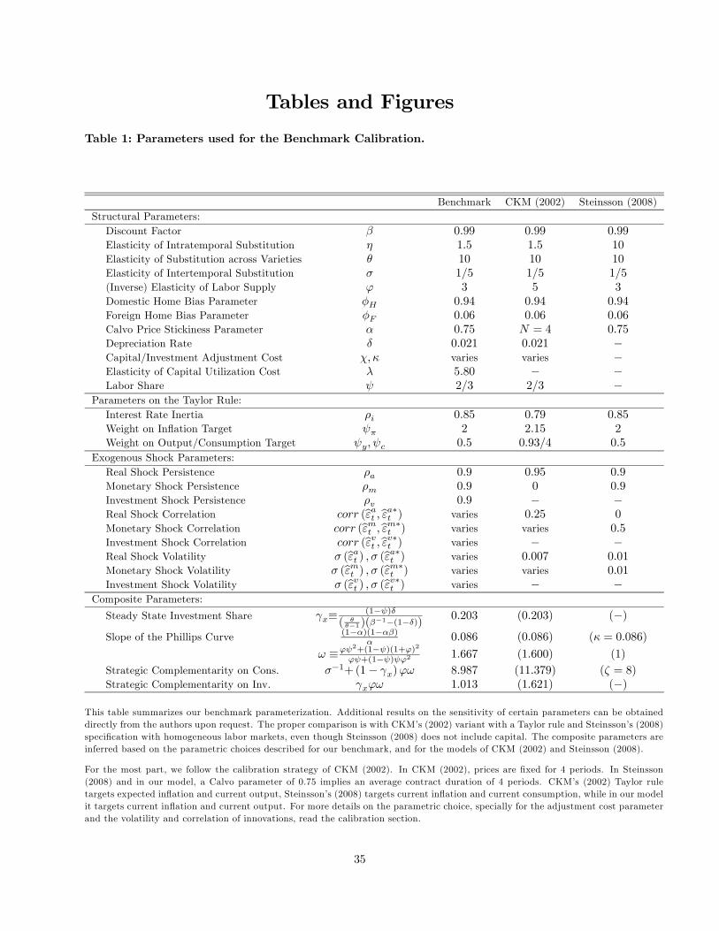
Tables and Figures

Table 1: Parameters used for the Benchmark Calibration.

Benchmark CKM (2002) Steinsson (2008)Structural Parameters:Discount Factor β 0.99 0.99 0.99Elasticity of Intratemporal Substitution η 1.5 1.5 10Elasticity of Substitution across Varieties θ 10 10 10Elasticity of Intertemporal Substitution σ 1/5 1/5 1/5(Inverse) Elasticity of Labor Supply ϕ 3 5 3Domestic Home Bias Parameter φH 0.94 0.94 0.94Foreign Home Bias Parameter φF 0.06 0.06 0.06Calvo Price Stickiness Parameter α 0.75 N = 4 0.75Depreciation Rate δ 0.021 0.021 −Capital/Investment Adjustment Cost χ, κ varies varies −Elasticity of Capital Utilization Cost λ 5.80 − −Labor Share ψ 2/3 2/3 −

Parameters on the Taylor Rule:Interest Rate Inertia ρi 0.85 0.79 0.85Weight on Inflation Target ψπ 2 2.15 2Weight on Output/Consumption Target ψy, ψc 0.5 0.93/4 0.5

Exogenous Shock Parameters:Real Shock Persistence ρa 0.9 0.95 0.9Monetary Shock Persistence ρm 0.9 0 0.9Investment Shock Persistence ρv 0.9 − −Real Shock Correlation corr (bεat ,bεa∗t ) varies 0.25 0Monetary Shock Correlation corr (bεmt ,bεm∗t ) varies varies 0.5Investment Shock Correlation corr (bεvt ,bεv∗t ) varies − −Real Shock Volatility σ (bεat ) , σ (bεa∗t ) varies 0.007 0.01Monetary Shock Volatility σ (bεmt ) , σ (bεm∗t ) varies varies 0.01Investment Shock Volatility σ (bεvt ) , σ (bεv∗t ) varies − −

Composite Parameters:

Steady State Investment Share γx≡(1−ψ)δ

( θθ−1)(β−1−(1−δ))

0.203 (0.203) (−)

Slope of the Phillips Curve (1−α)(1−αβ)α 0.086 (0.086) (κ = 0.086)

ω ≡ϕψ2+(1−ψ)(1+ϕ)2ϕψ+(1−ψ)ψϕ2 1.667 (1.600) (1)

Strategic Complementarity on Cons. σ−1+(1− γx)ϕω 8.987 (11.379) (ζ = 8)Strategic Complementarity on Inv. γxϕω 1.013 (1.621) (−)

This table summarizes our benchmark parameterization. Additional results on the sensitivity of certain parameters can be obtaineddirectly from the authors upon request. The proper comparison is with CKM’s (2002) variant with a Taylor rule and Steinsson’s (2008)specification with homogeneous labor markets, even though Steinsson (2008) does not include capital. The composite parameters areinferred based on the parametric choices described for our benchmark, and for the models of CKM (2002) and Steinsson (2008).

For the most part, we follow the calibration strategy of CKM (2002). In CKM (2002), prices are fixed for 4 periods. In Steinsson(2008) and in our model, a Calvo parameter of 0.75 implies an average contract duration of 4 periods. CKM’s (2002) Taylor ruletargets expected inflation and current output, Steinsson’s (2008) targets current inflation and current consumption, while in our modelit targets current inflation and current output. For more details on the parametric choice, specially for the adjustment cost parameterand the volatility and correlation of innovations, read the calibration section.

35

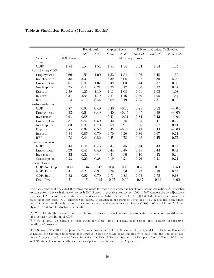
Table 2: Simulation Results (Monetary Shocks).

Benchmark Capital Specs. Effects of Capital UtilizationIAC NoC CAC NAC IAC+CU CAC+CU NAC+CU

Variable U.S. Data Monetary ShocksStd. dev.GDP∗ 1.54 1.54 1.54 1.54 1.54 1.54 1.54 1.54

Std. dev. to GDPEmployment 0.66 1.56 1.00 1.53 1.54 1.26 1.40 1.55Investment∗∗ 3.38 3.39 − 3.39 5.08 3.37 3.39 5.09Consumption 0.81 0.81 1.07 0.49 0.03 0.44 0.37 0.03Net Exports 0.25 0.40 0.21 0.25 0.17 0.30 0.22 0.17Exports 2.59 1.25 1.10 1.13 1.08 1.01 1.03 1.08Imports 3.31 3.54 1.79 2.21 1.46 2.60 1.90 1.47RER 5.14 5.13 6.44 3.09 0.19 2.65 2.31 0.19

AutocorrelationGDP 0.87 0.62 0.49 0.40 −0.05 0.75 0.52 −0.04Employment 0.92 0.64 0.49 0.40 −0.05 0.67 0.38 −0.05Investment 0.91 0.88 − 0.43 −0.04 0.84 0.42 −0.04Consumption 0.87 0.42 0.50 0.42 0.78 0.35 0.41 0.78Net Exports 0.83 0.86 0.70 0.69 0.21 0.86 0.67 0.21Exports 0.85 0.69 0.52 0.45 −0.03 0.72 0.44 −0.03Imports 0.84 0.87 0.70 0.70 0.20 0.86 0.67 0.21RER 0.78 0.44 0.52 0.45 0.78 0.38 0.45 0.77

Cross-correlationGDP∗ 0.44 0.44 0.46 0.44 0.45 0.44 0.44 0.44Employment 0.29 0.43 0.46 0.44 0.45 0.45 0.44 0.44Investment 0.33 0.02 − 0.24 0.30 0.10 0.25 0.29Consumption 0.33 0.20 0.28 0.19 0.21 0.26 0.21 0.21

CorrelationsGDP, Net Exp. −0.47 −0.45 −0.47 −0.46 −0.49 −0.49 −0.50 −0.50GDP, Exp. 0.41 0.20 0.34 0.29 0.36 0.22 0.29 0.34GDP, Imp. 0.82 0.62 0.79 0.73 0.88 0.68 0.78 0.88Exp., Imp. 0.21 −0.51 −0.13 −0.27 −0.00 −0.47 −0.24 −0.02

This table reports the selected theoretical moments for each series given our benchmark parameterization. All statisticsare computed after each simulated series is H-P filtered (smoothing parameter=1600). NAC denotes the no adjustmentcost case, CAC denotes the capital adjustment cost case (which is used in CKM (2002)), IAC denotes the investmentadjustment cost case, +CU indicates that capital utilization in the spirit of Christiano et al. (2005) has been added,and NoC identifies the only variant considered without capital (similar to Steinsson (2008)). We use Matlab 7.4.0 andDynare v3.051 for the stochastic simulation.

(*) We calibrate the volatility and correlation of monetary shock innovations to match the observed volatility andcross-country correlation of GDP.(**) We calibrate the adjustment cost parameter, if the model specification affords us one, to match the observedvolatility of investment.

Data Sources: The OECD’s Quarterly National Accounts, OECD’s Economic Outlook, and OECD’s Main EconomicIndicators are the most important data sources. Some series are complemented with data from the Bureau of Eco-nomic Analysis, the Bureau of Labor Statistics, the Federal Reserve System, the European Central Bank (ECB), andWM/Reuters. For more details, see the description of the dataset in the Appendix.

36

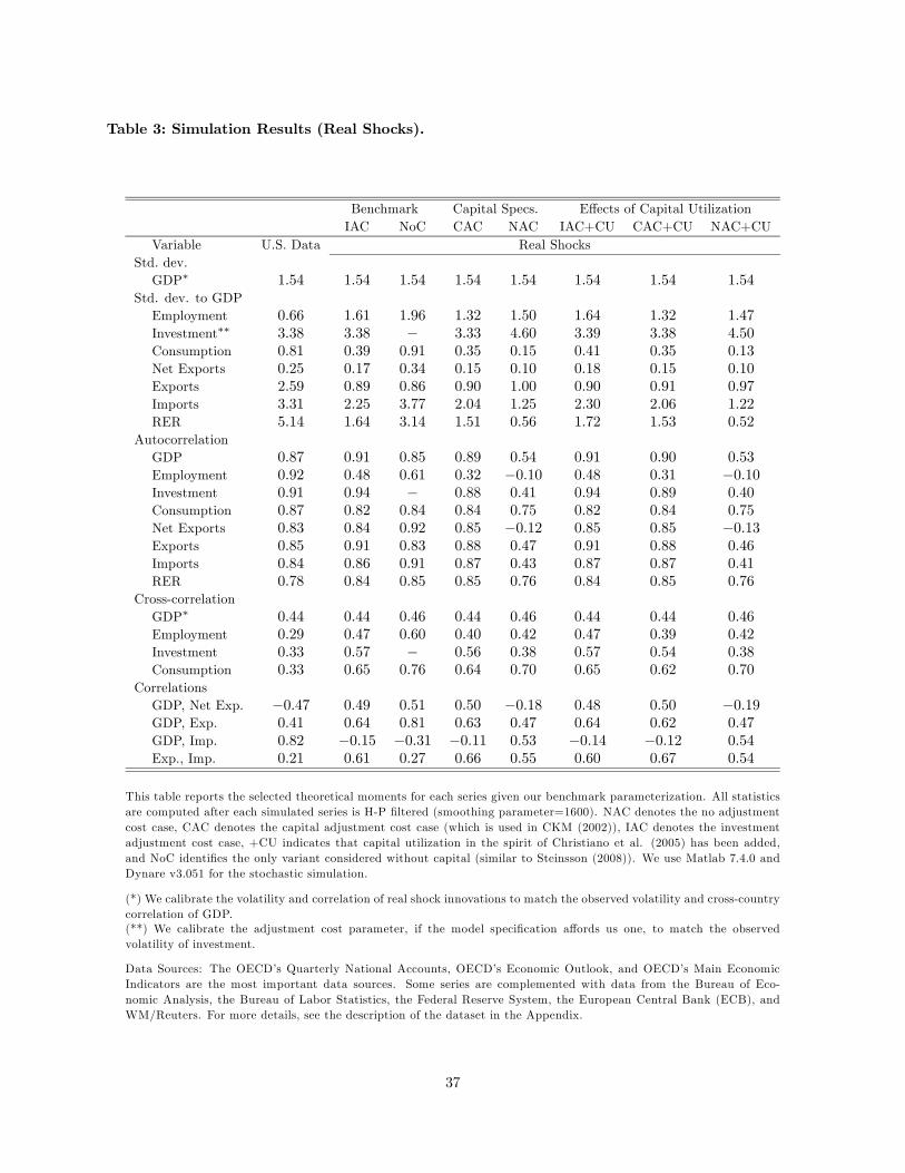
Table 3: Simulation Results (Real Shocks).

Benchmark Capital Specs. Effects of Capital UtilizationIAC NoC CAC NAC IAC+CU CAC+CU NAC+CU

Variable U.S. Data Real ShocksStd. dev.GDP∗ 1.54 1.54 1.54 1.54 1.54 1.54 1.54 1.54

Std. dev. to GDPEmployment 0.66 1.61 1.96 1.32 1.50 1.64 1.32 1.47Investment∗∗ 3.38 3.38 − 3.33 4.60 3.39 3.38 4.50Consumption 0.81 0.39 0.91 0.35 0.15 0.41 0.35 0.13Net Exports 0.25 0.17 0.34 0.15 0.10 0.18 0.15 0.10Exports 2.59 0.89 0.86 0.90 1.00 0.90 0.91 0.97Imports 3.31 2.25 3.77 2.04 1.25 2.30 2.06 1.22RER 5.14 1.64 3.14 1.51 0.56 1.72 1.53 0.52

AutocorrelationGDP 0.87 0.91 0.85 0.89 0.54 0.91 0.90 0.53Employment 0.92 0.48 0.61 0.32 −0.10 0.48 0.31 −0.10Investment 0.91 0.94 − 0.88 0.41 0.94 0.89 0.40Consumption 0.87 0.82 0.84 0.84 0.75 0.82 0.84 0.75Net Exports 0.83 0.84 0.92 0.85 −0.12 0.85 0.85 −0.13Exports 0.85 0.91 0.83 0.88 0.47 0.91 0.88 0.46Imports 0.84 0.86 0.91 0.87 0.43 0.87 0.87 0.41RER 0.78 0.84 0.85 0.85 0.76 0.84 0.85 0.76

Cross-correlationGDP∗ 0.44 0.44 0.46 0.44 0.46 0.44 0.44 0.46Employment 0.29 0.47 0.60 0.40 0.42 0.47 0.39 0.42Investment 0.33 0.57 − 0.56 0.38 0.57 0.54 0.38Consumption 0.33 0.65 0.76 0.64 0.70 0.65 0.62 0.70

CorrelationsGDP, Net Exp. −0.47 0.49 0.51 0.50 −0.18 0.48 0.50 −0.19GDP, Exp. 0.41 0.64 0.81 0.63 0.47 0.64 0.62 0.47GDP, Imp. 0.82 −0.15 −0.31 −0.11 0.53 −0.14 −0.12 0.54Exp., Imp. 0.21 0.61 0.27 0.66 0.55 0.60 0.67 0.54

This table reports the selected theoretical moments for each series given our benchmark parameterization. All statisticsare computed after each simulated series is H-P filtered (smoothing parameter=1600). NAC denotes the no adjustmentcost case, CAC denotes the capital adjustment cost case (which is used in CKM (2002)), IAC denotes the investmentadjustment cost case, +CU indicates that capital utilization in the spirit of Christiano et al. (2005) has been added,and NoC identifies the only variant considered without capital (similar to Steinsson (2008)). We use Matlab 7.4.0 andDynare v3.051 for the stochastic simulation.

(*) We calibrate the volatility and correlation of real shock innovations to match the observed volatility and cross-countrycorrelation of GDP.(**) We calibrate the adjustment cost parameter, if the model specification affords us one, to match the observedvolatility of investment.

Data Sources: The OECD’s Quarterly National Accounts, OECD’s Economic Outlook, and OECD’s Main EconomicIndicators are the most important data sources. Some series are complemented with data from the Bureau of Eco-nomic Analysis, the Bureau of Labor Statistics, the Federal Reserve System, the European Central Bank (ECB), andWM/Reuters. For more details, see the description of the dataset in the Appendix.

37

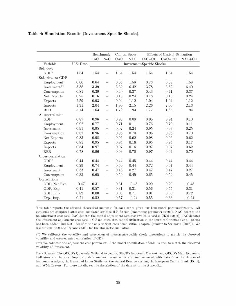
Table 4: Simulation Results (Investment-Specific Shocks).

Benchmark Capital Specs. Effects of Capital UtilizationIAC NoC CAC NAC IAC+CU CAC+CU NAC+CU

Variable U.S. Data Investment-Specific ShocksStd. dev.GDP∗ 1.54 1.54 − 1.54 1.54 1.54 1.54 1.54

Std. dev. to GDPEmployment 0.66 0.64 − 0.65 1.58 0.73 0.68 1.58Investment∗∗ 3.38 3.39 − 3.39 6.42 3.78 3.82 6.40Consumption 0.81 0.39 − 0.40 0.37 0.43 0.41 0.37Net Exports 0.25 0.16 − 0.15 0.24 0.18 0.15 0.24Exports 2.59 0.93 − 0.94 1.12 1.04 1.04 1.12Imports 3.31 2.04 − 1.90 2.15 2.26 2.00 2.13RER 5.14 1.63 − 1.79 1.93 1.77 1.85 1.94

AutocorrelationGDP 0.87 0.96 − 0.95 0.08 0.95 0.94 0.10Employment 0.92 0.77 − 0.71 0.11 0.76 0.70 0.11Investment 0.91 0.95 − 0.92 0.24 0.95 0.93 0.25Consumption 0.87 0.96 − 0.96 0.70 0.95 0.96 0.70Net Exports 0.83 0.98 − 0.96 0.62 0.98 0.96 0.62Exports 0.85 0.95 − 0.94 0.16 0.95 0.95 0.17Imports 0.84 0.97 − 0.97 0.16 0.97 0.97 0.62RER 0.78 0.96 − 0.93 0.70 0.97 0.94 0.70

Cross-correlationGDP∗ 0.44 0.44 − 0.44 0.45 0.44 0.44 0.44Employment 0.29 0.74 − 0.69 0.44 0.72 0.67 0.44Investment 0.33 0.47 − 0.48 0.27 0.47 0.47 0.27Consumption 0.33 0.65 − 0.59 0.45 0.65 0.59 0.45

CorrelationsGDP, Net Exp. −0.47 0.31 − 0.31 −0.45 0.29 0.29 −0.45GDP, Exp. 0.41 0.57 − 0.31 0.31 0.56 0.55 0.31GDP, Imp. 0.82 0.00 − 0.03 0.71 0.01 0.06 0.72Exp., Imp. 0.21 0.52 − 0.57 −0.24 0.55 0.63 −0.24

This table reports the selected theoretical moments for each series given our benchmark parameterization. Allstatistics are computed after each simulated series is H-P filtered (smoothing parameter=1600). NAC denotes theno adjustment cost case, CAC denotes the capital adjustment cost case (which is used in CKM (2002)), IAC denotesthe investment adjustment cost case, +CU indicates that capital utilization in the spirit of Christiano et al. (2005)has been added, and NoC identifies the only variant considered without capital (similar to Steinsson (2008)). Weuse Matlab 7.4.0 and Dynare v3.051 for the stochastic simulation.

(*) We calibrate the volatility and correlation of investment-specific shock innovations to match the observedvolatility and cross-country correlation of GDP.(**) We calibrate the adjustment cost parameter, if the model specification affords us one, to match the observedvolatility of investment.

Data Sources: The OECD’s Quarterly National Accounts, OECD’s Economic Outlook, and OECD’s Main EconomicIndicators are the most important data sources. Some series are complemented with data from the Bureau ofEconomic Analysis, the Bureau of Labor Statistics, the Federal Reserve System, the European Central Bank (ECB),and WM/Reuters. For more details, see the description of the dataset in the Appendix.

38

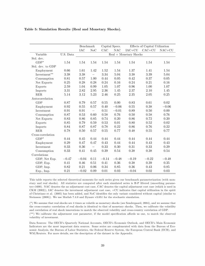
Table 5: Simulation Results (Real and Monetary Shocks).

Benchmark Capital Specs. Effects of Capital UtilizationIAC NoC CAC NAC IAC+CU CAC+CU NAC+CU

Variable U.S. Data Real + Monetary ShocksStd. dev.GDP∗ 1.54 1.54 1.54 1.54 1.54 1.54 1.54 1.54

Std. dev. to GDPEmployment 0.66 1.61 1.42 1.52 1.54 1.37 1.41 1.54Investment∗∗ 3.38 3.38 − 3.34 5.04 3.38 3.39 5.04Consumption 0.81 0.57 1.00 0.44 0.05 0.42 0.37 0.05Net Exports 0.25 0.28 0.28 0.24 0.16 0.24 0.21 0.16Exports 2.59 1.04 0.99 1.05 1.07 0.96 1.00 1.07Imports 3.31 2.82 2.95 2.36 1.45 2.37 2.10 1.45RER 5.14 3.12 5.23 2.46 0.25 2.35 2.05 0.25

AutocorrelationGDP 0.87 0.79 0.57 0.55 0.00 0.83 0.61 0.02Employment 0.92 0.55 0.57 0.40 −0.06 0.55 0.38 −0.06Investment 0.91 0.91 − 0.51 −0.01 0.89 0.50 0.00Consumption 0.87 0.53 0.60 0.58 0.76 0.50 0.58 0.76Net Exports 0.83 0.86 0.85 0.74 0.20 0.86 0.72 0.20Exports 0.85 0.79 0.59 0.53 0.01 0.80 0.52 0.02Imports 0.84 0.87 0.87 0.78 0.22 0.86 0.76 0.22RER 0.78 0.50 0.57 0.55 0.77 0.48 0.55 0.77

Cross-correlationGDP∗ 0.44 0.45 0.44 0.44 0.44 0.44 0.44 0.44Employment 0.29 0.47 0.47 0.43 0.44 0.44 0.43 0.43Investment 0.33 0.36 − 0.33 0.30 0.31 0.33 0.29Consumption 0.33 0.41 0.45 0.39 0.54 0.38 0.38 0.54

CorrelationsGDP, Net Exp. −0.47 −0.04 0.11 −0.14 −0.48 −0.19 −0.22 −0.48GDP, Exp. 0.41 0.46 0.51 0.41 0.36 0.38 0.39 0.35GDP, Imp. 0.82 0.21 0.06 0.34 0.85 0.36 0.43 0.85Exp., Imp. 0.21 −0.02 0.09 0.01 0.03 −0.04 0.02 0.03

This table reports the selected theoretical moments for each series given our benchmark parameterization (with mon-etary and real shocks). All statistics are computed after each simulated series is H-P filtered (smoothing parame-ter=1600). NAC denotes the no adjustment cost case, CAC denotes the capital adjustment cost case (which is used inCKM (2002)), IAC denotes the investment adjustment cost case, +CU indicates that capital utilization in the spiritof Christiano et al. (2005) has been added, and NoC identifies the only variant considered without capital (similar toSteinsson (2008)). We use Matlab 7.4.0 and Dynare v3.051 for the stochastic simulation.

(*) We assume that real shocks are 4 times as volatile as monetary shocks (see Søndergaard, 2004), and we assume thatthe cross-country correlation of real shocks is identical to that of monetary shocks. Then, we calibrate the volatilityand correlation of real shock innovations to match the observed volatility and cross-country correlation of GDP.(**) We calibrate the adjustment cost parameter, if the model specification affords us one, to match the observedvolatility of investment.

Data Sources: The OECD’s Quarterly National Accounts, OECD’s Economic Outlook, and OECD’s Main EconomicIndicators are the most important data sources. Some series are complemented with data from the Bureau of Eco-nomic Analysis, the Bureau of Labor Statistics, the Federal Reserve System, the European Central Bank (ECB), andWM/Reuters. For more details, see the description of the dataset in the Appendix.

39

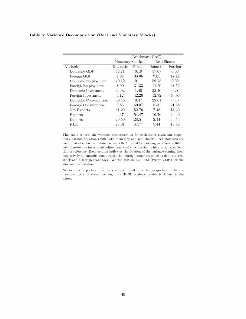
Table 6: Variance Decomposition (Real and Monetary Shocks).

Benchmark (IAC)Monetary Shocks Real Shocks

Variable Domestic Foreign Domestic ForeignDomestic GDP 42.71 0.19 57.07 0.03Foreign GDP 9.84 33.06 9.68 47.42Domestic Employment 40.12 0.11 59.75 0.02Foreign Employment 8.90 31.33 11.26 48.52Domestic Investment 44.92 1.40 53.40 0.28Foreign Investment 4.12 42.20 12.72 40.96Domestic Consumption 69.46 0.47 29.61 0.46Foreign Consumption 9.85 60.07 8.50 21.58Net Exports 21.29 52.76 7.46 18.49Exports 4.37 54.47 16.76 24.40Imports 29.50 28.51 2.44 39.54RER 23.31 57.77 5.44 13.48

This table reports the variance decomposition for each series given our bench-mark parameterization (with both monetary and real shocks). All statistics arecomputed after each simulated series is H-P filtered (smoothing parameter=1600).IAC denotes the investment adjustment cost specification, which is our specifica-tion of reference. Each column indicates the fraction of the variance coming fromrespectively a domestic monetary shock, a foreign monetary shock, a domestic realshock and a foreign real shock. We use Matlab 7.4.0 and Dynare v3.051 for thestochastic simulation.

Net exports, exports and imports are computed from the perspective of the do-mestic country. The real exchange rate (RER) is also consistently defined in thepaper.

40

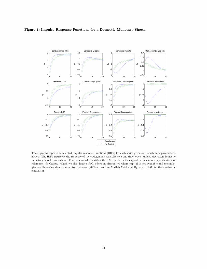
Figure 1: Impulse Response Functions for a Domestic Monetary Shock.

0 10 20-6

-4

-2

0Real Exchange Rate

%

0 10 20-0.6

-0.4

-0.2

0

0.2Domestic Exports

%0 10 20

-3

-2

-1

0

1Domestic Imports

%

0 10 20-0.05

0

0.05

0.1

0.15

0.2Domestic Net Exports

%

0 10 20-1.5

-1

-0.5

0Domestic GDP

%

0 10 20-2

-1

0

1Domestic Employment

%

0 10 20-2

-1.5

-1

-0.5

0Domestic Consumption

%0 10 20

-4

-3

-2

-1

0Domestic Investment

%0 10 20

-0.8

-0.6

-0.4

-0.2

0Foreign GDP

%

0 10 20-0.8

-0.6

-0.4

-0.2

0Foreign Employment

%

0 10 20-0.6

-0.4

-0.2

0

0.2Foreign Consumption

%

0 10 20-0.8

-0.6

-0.4

-0.2

0Foreign Investment

%

BenchmarkNo Capital

These graphs report the selected impulse response functions (IRFs) for each series given our benchmark parameteri-zation. The IRFs represent the response of the endogenous variables to a one time, one standard deviation domesticmonetary shock innovation. The benchmark identifies the IAC model with capital, which is our specification ofreference. No Capital, which we also denote NoC, offers an alternative where capital is not available and technolo-gies are linear-in-labor (similar to Steinsson (2008)). We use Matlab 7.4.0 and Dynare v3.051 for the stochasticsimulation.

41

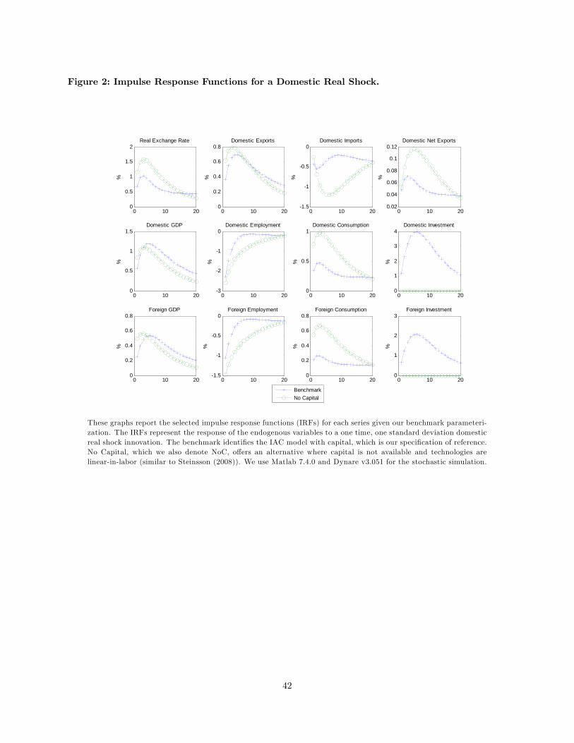
Figure 2: Impulse Response Functions for a Domestic Real Shock.

0 10 200

0.5

1

1.5

2Real Exchange Rate

%

0 10 200

0.2

0.4

0.6

0.8Domestic Exports

%0 10 20

-1.5

-1

-0.5

0Domestic Imports

%

0 10 200.02

0.04

0.06

0.08

0.1

0.12Domestic Net Exports

%

0 10 200

0.5

1

1.5Domestic GDP

%

0 10 20-3

-2

-1

0Domestic Employment

%

0 10 200

0.5

1Domestic Consumption

%0 10 20

0

1

2

3

4Domestic Investment

%0 10 20

0

0.2

0.4

0.6

0.8Foreign GDP

%

0 10 20-1.5

-1

-0.5

0Foreign Employment

%

0 10 200

0.2

0.4

0.6

0.8Foreign Consumption

%

0 10 200

1

2

3Foreign Investment

%

BenchmarkNo Capital

These graphs report the selected impulse response functions (IRFs) for each series given our benchmark parameteri-zation. The IRFs represent the response of the endogenous variables to a one time, one standard deviation domesticreal shock innovation. The benchmark identifies the IAC model with capital, which is our specification of reference.No Capital, which we also denote NoC, offers an alternative where capital is not available and technologies arelinear-in-labor (similar to Steinsson (2008)). We use Matlab 7.4.0 and Dynare v3.051 for the stochastic simulation.

42

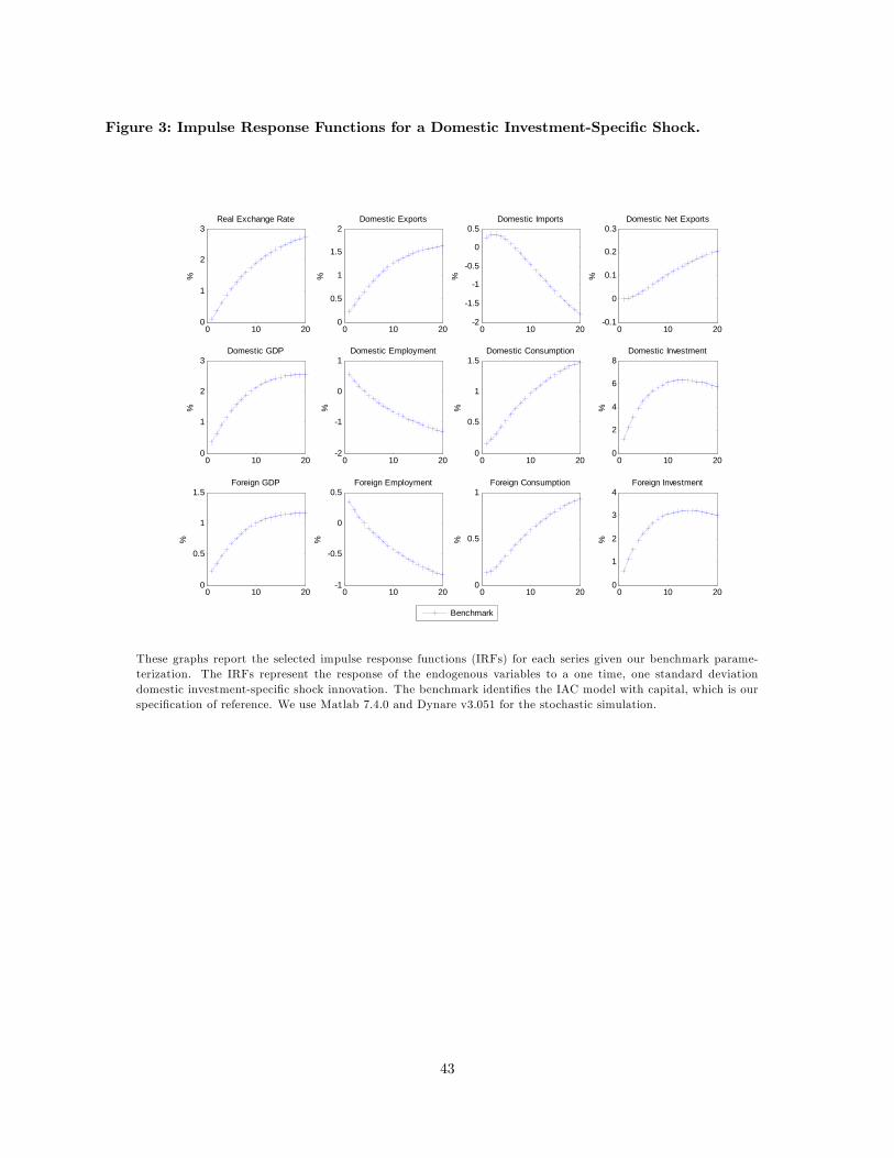
Figure 3: Impulse Response Functions for a Domestic Investment-Specific Shock.

0 10 200

1

2

3Real Exchange Rate

%

0 10 200

0.5

1

1.5

2Domestic Exports

%0 10 20

-2

-1.5

-1

-0.5

0

0.5Domestic Imports

%

0 10 20-0.1

0

0.1

0.2

0.3Domestic Net Exports

%

0 10 200

1

2

3Domestic GDP

%

0 10 20-2

-1

0

1Domestic Employment

%

0 10 200

0.5

1

1.5Domestic Consumption

%0 10 20

0

2

4

6

8Domestic Investment

%0 10 20

0

0.5

1

1.5Foreign GDP

%

0 10 20-1

-0.5

0

0.5Foreign Employment

%

0 10 200

0.5

1Foreign Consumption

%

0 10 200

1

2

3

4Foreign Investment

%

Benchmark

These graphs report the selected impulse response functions (IRFs) for each series given our benchmark parame-terization. The IRFs represent the response of the endogenous variables to a one time, one standard deviationdomestic investment-specific shock innovation. The benchmark identifies the IAC model with capital, which is ourspecification of reference. We use Matlab 7.4.0 and Dynare v3.051 for the stochastic simulation.

43