1

The Proportional Odds Model for Assessing Rater Agreement with Multiple

Modalities

Elizabeth Garrett-Mayer, PhD

Assistant ProfessorSidney Kimmel Comprehensive Cancer Center

Johns Hopkins University

2

Learning Objectives

1) the need for standardized classification systems for cancer

2) the definition of a latent variable3) the framework of the proportional odds

model and its application to categorical ratings

4) the interpretation of rater effects and utility of the model for describing reliability of rating system

3

The Motivation

• Histologic classification systems help in understanding of cancer progression

• In some types of cancers, classification systems have only recently occurred

• Classification system necessary to facilitate research– Clinical– Pathologic– molecular

4

The Motivation

• Proliferative epithelial lesions in the smaller pancreatic cancer ducts (Hruban et al. (2001): American Journal of Surgical Pathology)

• Complex study design– First stage:

• 8 pathologists• 35 microscopic slides• Results: Over 70 different diagnostic terms

5

The Motivation

• Complex study design– Second stage: Development of Pan-IN

• Two classification schemes developed (next slide)– Illustrations– nomenclature

• Same 8 pathologists (raters)• Same 35 slides• Each rater evaluated each slide twice

(nomenclature and illustrations)• Blinded between ratings

6

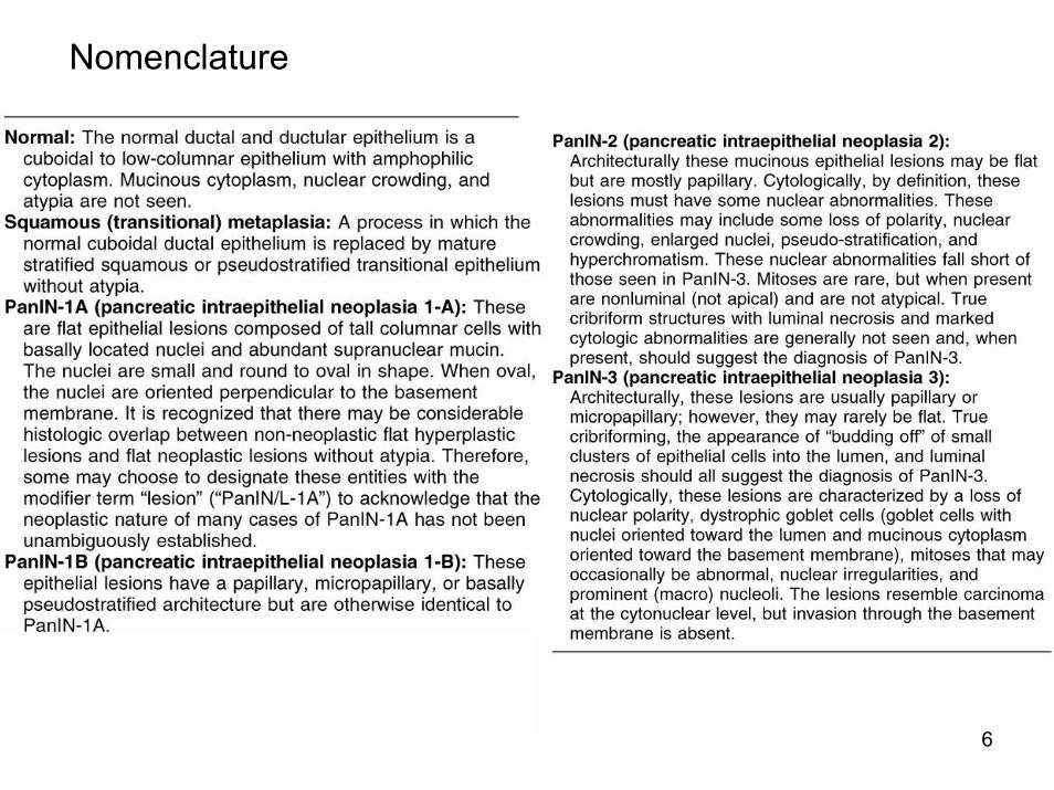
Nomenclature

7

(A) Normal duct.

(B and C) Squamousmetaplasia.

(D–I) PanIN-1A.

(J–O) PanIN-1B.

8

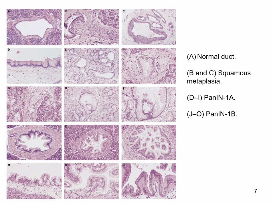
(A–F) PanIN-2.

(G–L) PanIN-3.

(M) Intraductal papillary mucinous neoplasm.

(N–O) Invasive adenocarcinomasecondarily involving a duct (cancerizationof the ducts).

9

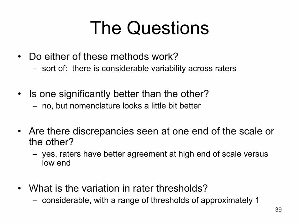
The Questions• Do either of these methods work?

• Is one significantly better than the other?

• Are there discrepancies seen at one end of the scale or the other?

• What is the variation across raters?

10

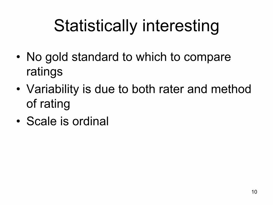
Statistically interesting

• No gold standard to which to compare ratings

• Variability is due to both rater and method of rating

• Scale is ordinal

11

Exploit as a latent variable problem

• Is cancer progression really “categorical”?• More likely continuous• Categories represent imposition of

“thresholds”• Questions rephrased:

– Do raters have different thresholds?– What is the variance of the thresholds?– Do thresholds and their variances vary across

methods?

12

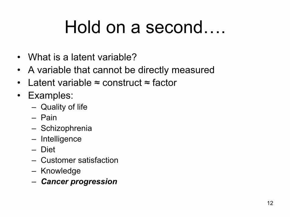
Hold on a second….• What is a latent variable?• A variable that cannot be directly measured• Latent variable ≈ construct ≈ factor • Examples:

– Quality of life– Pain– Schizophrenia– Intelligence– Diet– Customer satisfaction– Knowledge– Cancer progression

13

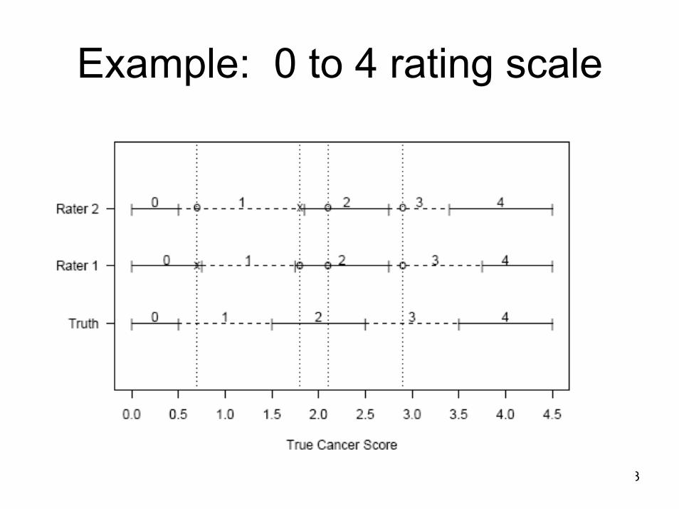
Example: 0 to 4 rating scale

14

Latent Variable Approach

• Treat underlying cancer progression as continuous

• Assume that ratings are ordinal and that raters “round” their ratings to nearest integer

• Estimate the thresholds of raters

15

Other approaches?• Kappa?

– Measures agreement– Can handle ordinal or categorical ratings– Can handle multiple raters– Or, can handle multiple modalities– Cannot handle both multiple raters and modalities– Can use kappa to

• Estimate separate agreements for the two approaches• Estimate overall agreement, ignoring method of rating

– Not ideal:• Does not allow us to compare methods directly• Does not allow us to assess differences due to rater effects

versus variance.• Does not acknowledge underlying continuous variable• “black box”

16

Other approaches• Tanner and Young (1985), Becker and Agresti

(1992), Perkins and Becker (2002)– log-linear model – Partition observed data into agreement and chance

components– Model pairwise agreements

• Do pairs of raters have same agreement structure?• Do raters have same aggregate level of agreement with other

raters?– Problems:

• not extended to deal with multiple modalities• treats data as nominal• Does not acknowledge latent variable problem

17

Other approaches• Agresti (1988)

– Extends Tanner and Young (1985) treating data as ordinal

– Latent class variable approach– Problem: does not acknowledge continuity

• Uebersax and Grove (1993)– Latent trait mixture model– Assumes binary classification is goal– Problems:

• Imposes strong normality assumptions• Does not acknowledge continuity

18

Other approaches

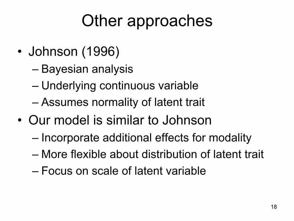
• Johnson (1996)– Bayesian analysis– Underlying continuous variable– Assumes normality of latent trait

• Our model is similar to Johnson– Incorporate additional effects for modality– More flexible about distribution of latent trait– Focus on scale of latent variable

19

The proportional odds model

• McCullagh (1980)• AKA “ordinal logistic regression”• Developed to deal with thresholded data• Goal was to estimate the association

between some risk factors and an ordinal outcome of interest

• Assumes that there is a ‘proportional’ increase in risk.

20

The proportional odds model (POM)

log( )( )

,...,P Y kP Y k

x k Ki

ii k

>≤

= + = −β α ; 1 1

• Example: – Outcome: “how is your health?” (5=excellent, 4=very

good, 3=good, 2=fair, 1=poor)– Predictor: diabetes (1=yes, 0=no)

• β: log odds ratio of higher rating for diabetics versus non-diabetics (2,3,4,5 vs. 1; 3,4,5 vs. 1,2 ; 4,5 vs. 1,2,3; 5 vs. 1,2,3,4)

• αk: nuisance parameter. calibration factor.

21

POM for rater agreement in Pan-IN

• βi: latent variable – represents true cancer progression for patient i

• αk: threshold parameters• Three categories:

– 1A and 1B lumped together– none were “normal”– also had an “other” category that is treated as missing (not ordinal)

• Two thresholds: between 1 and 2, and between 2 and 3.• Model must include

– rater effects (8 raters)– method effect (illustration versus nomenclature)

• Additional complication: latent variable?!

22

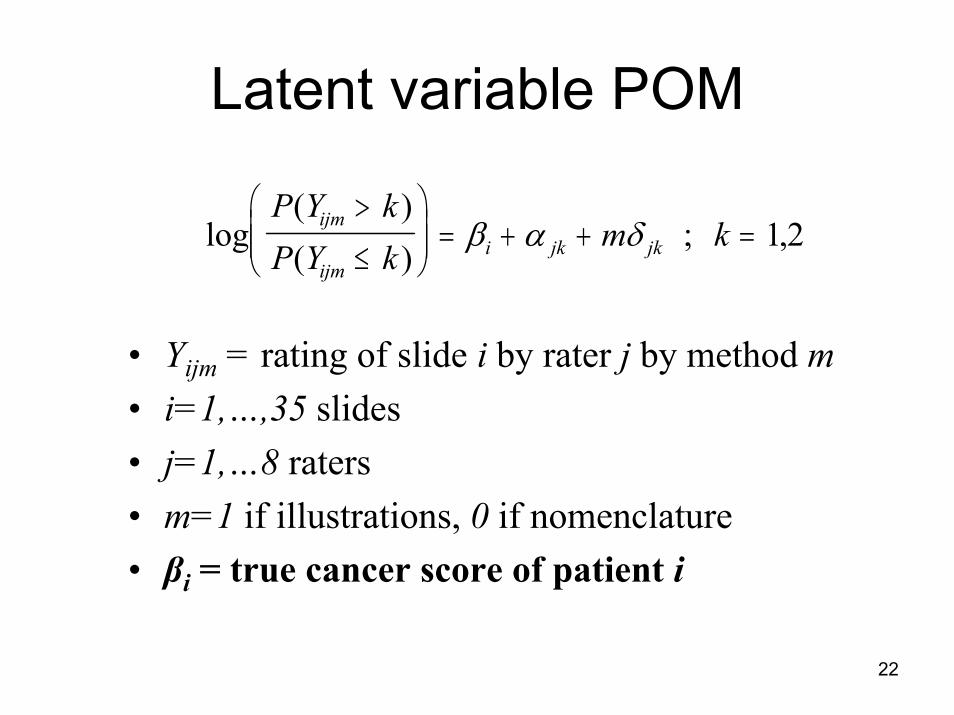
Latent variable POM

log( )( )

,P Y kP Y k

m kijm

ijmi jk jk

>

≤

= + + =β α δ ; 1 2

• Yijm = rating of slide i by rater j by method m• i=1,…,35 slides• j=1,…8 raters• m=1 if illustrations, 0 if nomenclature• βi = true cancer score of patient i

23

Latent variable POM

log( )( )

,P Y kP Y k

m kijm

ijmi jk jk

>

≤

= + + =β α δ ; 1 2

α

α

α δ

α δ

δ

δ

j

j

j j

j j

j

j

jj

jj

jj

1

2

1 1

2 2

1

2

::::::

lower nomenclature effect for rater upper nomenclature effect for rater lower illustrations effect for rater upper illustrations effect for rater difference between lower effects for rater difference between upper effects for rater

+

+

24

Model Assumptions and Estimation

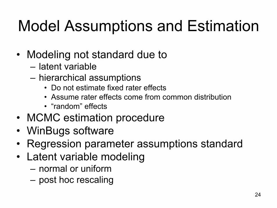
• Modeling not standard due to – latent variable– hierarchical assumptions

• Do not estimate fixed rater effects• Assume rater effects come from common distribution• “random” effects

• MCMC estimation procedure• WinBugs software• Regression parameter assumptions standard• Latent variable modeling

– normal or uniform– post hoc rescaling

25

Model Assumptions

α σ α

α α σ α

δ δ σ

β µ τ βα

σ

σ

α

α

δ

α

δ

j j

j j

jk k k

i i

k

k

N I

N I

N

N U a bN

GammaGamma

1 12

2

2 2 22

1

2

2

22

2

0

0 1001 0 01 0 01

1 0 01 0 01

~ ( , ) ( , )

~ ( , ) ( , )

~ ( , )

~ ( , ) ~ [ , ]~ ( , )

/ ~ ( . , . )

/ ~ ( . , . )

−∞

∞

or

26

Interpretation of βi

log( )( )

( )

log( )( )

$ ( )$

$

P YP Y

E

EP YP Y

P Ye

e

ij

iji j j

ij

iji

i

i

i

0

01 1

0

0

0

11

0

11

11

>

≤

= + =

⇒>

≤

=

⇒ > =+⋅

β α α

β

β

β

and

βi represents (on the logit scale) the probability that slide i is rated a 2 or a 3 by nomenclature.

Example: βi = 0 means that the estimated probability that slide i is a 2 or 3 is 0.50

27

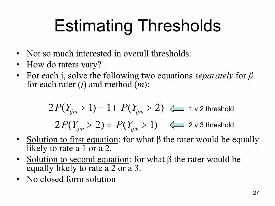
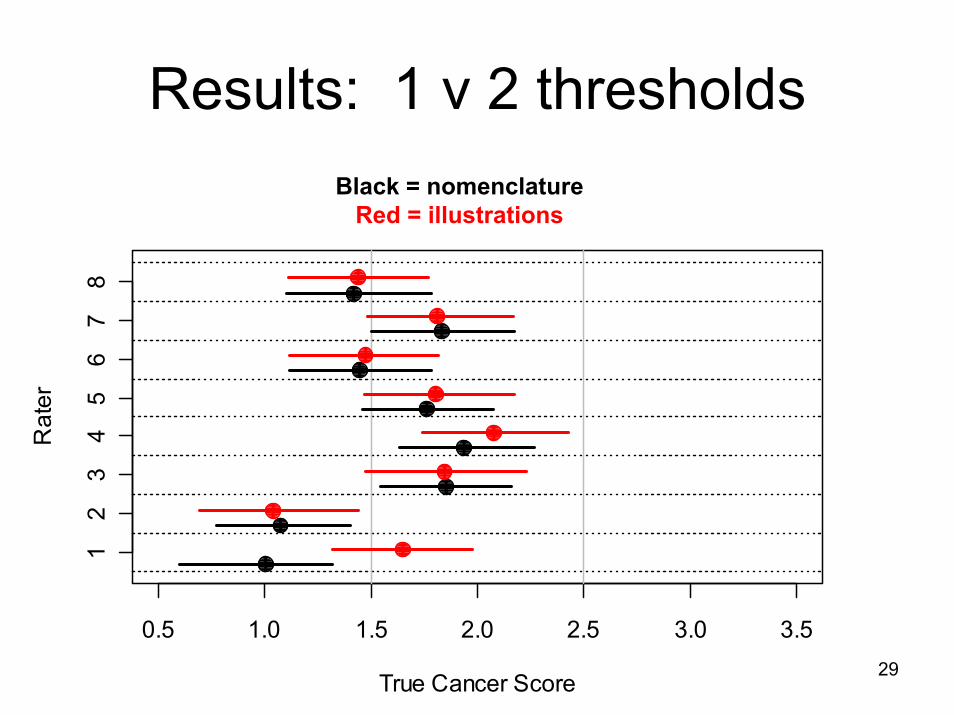
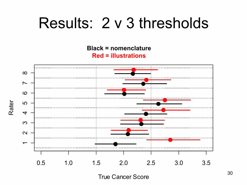
Estimating Thresholds• Not so much interested in overall thresholds.• How do raters vary?• For each j, solve the following two equations separately for β

for each rater (j) and method (m):

• Solution to first equation: for what β the rater would be equally likely to rate a 1 or a 2.

• Solution to second equation: for what β the rater would be equally likely to rate a 2 or a 3.

• No closed form solution

2 1 1 22 2 1P Y P Y

P Y P Yijm ijm

ijm ijm

( ) ( )( ) ( )

> = + >

> = >

1 v 2 threshold

2 v 3 threshold

28

Rescaling• Latent variable (β) is not in

scale of grading system• Most interpretable if

thresholds are in terms of original units

• Can we recalibrate?• Interpolation

– Assume linear relationship between β and empirical means

– Interpolate any other quantities on β-scale of interest

• Other approaches 1.0 1.5 2.0 2.5 3.0

-4-2

02

46

8

Empirical Score

Late

nt S

core

29

Results: 1 v 2 thresholdsBlack = nomenclature

Red = illustrations

0.5 1.0 1.5 2.0 2.5 3.0 3.5

True Cancer Score

Rat

er

12

34

56

78

30

Results: 2 v 3 thresholdsBlack = nomenclature

Red = illustrations

0.5 1.0 1.5 2.0 2.5 3.0 3.5

True Cancer Score

Rat

er

12

34

56

78

31

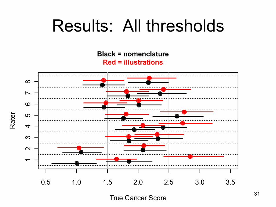
Results: All thresholdsBlack = nomenclature

Red = illustrations

0.5 1.0 1.5 2.0 2.5 3.0 3.5

True Cancer Score

Rat

er

12

34

56

78

32

Results: All thresholdsBlack = nomenclature

Red = illustrations

-5 0 5 10

True Cancer Score

Rat

er

12

34

56

78

33

Standard Deviation of Thresholds

0.5 1.0 1.5 2.0 2.5 3.0 3.5

0.0

0.2

0.4

0.6

0.8

1.0

1.2

Standard Deviation

Den

sity

Black = nomenclatureRed = illustrations

Solid = threshold 1 v 2Dashed = threshold 2 v 3

34

Anything look odd?

• Rater 1 had misunderstood the rating system for nomenclature

• Instead of coding PanIN 1A and 1B as “1”, he coded them as “1” and “2”, and PanIN2 as “3”, etc.

• Effect: his nomenclature ratings tend to be biased upwards

35

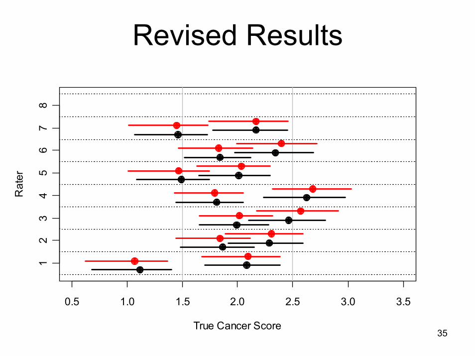
Revised Results

0.5 1.0 1.5 2.0 2.5 3.0 3.5

True Cancer Score

Rat

er

12

34

56

78

36

Revised Results

0.5 1.0 1.5 2.0 2.5 3.0

0.0

0.5

1.0

1.5

Standard Deviation

Den

sity

Black = nomenclatureRed = illustrations

Solid = threshold 1 v 2Dashed = threshold 2 v 3

37

Revised Results

• Standard Deviations across two methods look about the same as each other now– illustrations slightly higher– not ‘interestingly’ different

• Otherwise, things are similar– Rater thresholds were not sensitive to

exclusion– True cancer scores were not sensitive

38

Sensitivity Analysis

• Assumed distribution of β• Uniform versus Normal?• Inferences appear to be the same

39

The Questions• Do either of these methods work?

– sort of: there is considerable variability across raters

• Is one significantly better than the other?– no, but nomenclature looks a little bit better

• Are there discrepancies seen at one end of the scale or the other?– yes, raters have better agreement at high end of scale versus

low end

• What is the variation in rater thresholds?– considerable, with a range of thresholds of approximately 1

40

Interpretation• Both methods appear to perform approximately equally

well• Bias?

– Both methods taught simultaneously. – Better design:

• separate raters for each method• Teach rater only one method

• After removing rater 1, nomenclature looks slightly better• Large variability in rater thresholds• Greater variability in 1 vs. 2 than in 2 vs. 3• Suggests room for improvement

41

Utility of Model• Not only when multiple raters, multiple

modalities• If only nomenclature OR illustrations still would

have been useful• Some key ideas:

– Comparisons of rater thresholds– Assessment of variability of thresholds– Rescaling to original metric for interpretability

• Useful for any ordinal rating system where underlying variable can be considered continuous