Effect Displays for Multinomial and Proportional-Odds...
31
EFFECT DISPLAYS FOR MULTINOMIAL AND PROPORTIONAL-ODDS LOGIT MODELS John Fox* Robert Andersen* An “effect display” is a graphical or tabular summary of a statisti- cal model based on high-order terms in the model. Effect displays have previously been defined by Fox (1987, 2003) for generalized linear models (including linear models). Such displays are espe- cially compelling for complicated models—for example, those in- cluding interactions or polynomial terms. This paper extends effect displays to models commonly used for polytomous categorical re- sponse variables: the multinomial logit model and the proportional- odds logit model. Determining point estimates of effects for these models is a straightforward extension of results for the general- ized linear model. Estimating sampling variation for effects on the probability scale in the multinomial and proportional-odds logit models is more challenging, however, and we use the delta method to derive approximate standard errors. Finally, we provide software for effect displays in the R statistical computing environment. This is a revised version of a paper read at the ASA Methodology Confer- ence 2004. Please address correspondence to John Fox, Department of Sociology, McMaster University, 1280 Main Street West, Hamilton, Ontario, Canada L8S 4M4; [email protected]. We are grateful to Georges Monette for checking some of the derivations in this paper, and to Michael Ornstein and two anonymous reviewers for helpful suggestions. ∗ McMaster University 225
Transcript of Effect Displays for Multinomial and Proportional-Odds...

EFFECT DISPLAYS FORMULTINOMIAL ANDPROPORTIONAL-ODDS LOGITMODELS
John Fox*Robert Andersen*
An “effect display” is a graphical or tabular summary of a statisti-cal model based on high-order terms in the model. Effect displayshave previously been defined by Fox (1987, 2003) for generalizedlinear models (including linear models). Such displays are espe-cially compelling for complicated models—for example, those in-cluding interactions or polynomial terms. This paper extends effectdisplays to models commonly used for polytomous categorical re-sponse variables: the multinomial logit model and the proportional-odds logit model. Determining point estimates of effects for thesemodels is a straightforward extension of results for the general-ized linear model. Estimating sampling variation for effects on theprobability scale in the multinomial and proportional-odds logitmodels is more challenging, however, and we use the delta methodto derive approximate standard errors. Finally, we provide softwarefor effect displays in the R statistical computing environment.
This is a revised version of a paper read at the ASA Methodology Confer-ence 2004. Please address correspondence to John Fox, Department of Sociology,McMaster University, 1280 Main Street West, Hamilton, Ontario, Canada L8S4M4; [email protected]. We are grateful to Georges Monette for checking some ofthe derivations in this paper, and to Michael Ornstein and two anonymous reviewersfor helpful suggestions.
∗McMaster University
225

226 FOX AND ANDERSEN
1. INTRODUCTION
Effect displays, in the sense of Fox (1987, 2003), are tabular or—moreoften—graphical summaries of statistical models. Fox (1987) introduceseffect displays for generalized linear models (including linear models);Fox (2003) refines these methods and provides software for their essen-tially automatic implementation.
The general idea underlying effect displays—to represent a sta-tistical model by showing carefully selected portions of its responsesurface—is not limited to generalized linear models, however, nor evento models that incorporate linear predictors. Moreover, the essentialidea of effect displays is not wholly original with Fox (1987). For ex-ample, adjusted means in analysis of covariance (introduced by Fisher,1936) are a precursor to more general effect displays. Goodnight andHarvey’s (1978) “least-squares means” in analysis of variance and co-variance, and Searle, Speed, and Milliken’s (1980) “estimated popula-tion marginal means” are effect displays restricted to interactions amongfactors (i.e., categorical predictors) in a linear model.
King, Tomz, and Wittenberg (2000) and Tomz, Wittenberg, andKing (2003) have presented similar ideas, but their approach is basedon Monte-Carlo simulation of a model. In contrast, the analytical re-sults that we give below can be computed directly. Long (1997) discussesseveral strategies for presenting statistical models fit to categorical re-sponse variables, including displaying estimated probabilities. Hastie,Tibshirani, and Friedman’s (2001, sec. 10.13.2) “partial dependenceplots” and Weisberg’s (2005: 185–90) “marginal model plots” are alsorelated to effect displays.
The primary purpose of this paper is to extend the effect dis-plays in Fox (1987, 2003) to the multinomial logit model and to theproportional-odds logit model, statistical models that find common ap-plication in social research. As we will show, this extension is largelystraightforward, although the derivation of standard errors is challeng-ing, particularly in the proportional-odds model. We begin by reviewingeffect displays for generalized linear models, using as examples a binarylogit model and a linear model. We then present results for the multino-mial and proportional-odds logit models. In each of these sections, weillustrate the results with examples.
We see the main contribution of this paper as twofold: First,by extending the methods in Fox (1987, 2003) to models commonlyused for polytomous data, we provide a means for carefully visualizing

EFFECT DISPLAYS FOR LOGIT MODELS 227
models of this type that have complex structure, such as polynomialor spline regressors and interactions. Second, we derive standard er-rors for fitted probabilities in multinomial and proportional-odds logitmodels, permitting us to show statistical uncertainty in effect displaysconstructed for these models.
2. EFFECT DISPLAYS FOR GENERALIZED LINEARMODELS: BACKGROUND AND PRELIMINARY EXAMPLES
A general principle of interpretation for statistical models containingterms that are marginal to others (in the sense of Nelder 1977) is thathigh-order terms should be combined with their lower-order relatives—for example, an interaction between two factors should be combinedwith the main effects marginal to the interaction. In conformity withthis principle, Fox (1987) suggests identifying the high-order terms ina generalized linear model and computing fitted values for each suchterm. The lower-order “relatives” of a high-order term (e.g., main effectsmarginal to an interaction, or a linear and quadratic term in a third-order polynomial, which are marginal to the cubic term) are absorbedinto the term, allowing the predictors appearing in the high-order termto range over their values. The values of other predictors are fixed attypical values: For example, a covariate could be fixed at its mean ormedian, a factor at its proportional distribution in the data, or to equalproportions in its several levels.
Some models have high-order terms that “overlap”—that is, thatshare a lower-order relative (other than the constant). Consider, forexample, a generalized linear model that includes interactions AB, AC,and BC among the three factors A, B, and C. Although the three-wayinteraction ABC is not in the model, it is nevertheless illuminating tocombine the three high-order terms and their lower-order relatives (seeFox 2003 and the example developed in Section 2.1).
Let us turn now to the generalized linear model (e.g., McCullaghand Nelder 1989 or Firth 1991) with linear predictor η = Xβ and linkfunction g(µ) = η, where µ is the expectation of the response vector y.Here, everything falls into place very simply: We have an estimate β̂ of
β, along with the estimated covariance matrix ̂V(β̂) of β̂ .Let the rows of X∗ include all combinations of values of predic-
tors appearing in a high-order term, along with typical values of theremaining predictors. The structure of X∗ with respect, for example, to

228 FOX AND ANDERSEN
interactions, is the same as that of the model matrix X. Then the fittedvalues η̂∗ = X∗β̂ represent the effect in question, and a table or graphof these values—or, alternatively, of the fitted values transformed to thescale of the response, g−1 (η̂∗)—is an effect display. The standard errors
of η̂∗, available as the square-root diagonal entries of X∗ ̂V(β̂) X∗′, maybe used to compute pointwise confidence intervals for the effects, theendpoints of which may then also be transformed to the scale of theresponse.
In an application, as we will illustrate presently, we prefer plot-ting on the scale of the linear predictor (where the structure of themodel—for example, with respect to linearity—is preserved) but label-ing the response axis on the scale of the response. This approach hasthe advantage of making the configuration of the display invariant withrespect to the values at which the omitted predictors are held constant,in the sense that only the labeling of the response axis changes with adifferent selection of these values.1
2.1. A Binary Logit Model: Toronto Arrests for Marijuana Possession
Following Fox (2003), we construct effect displays for a binary logitmodel fit to data on police treatment of individuals arrested in Torontofor simple possession of small quantities of marijuana. (The data dis-cussed here are part of a larger data set featured in a series of articlesin the Toronto Star newspaper.) Under these circumstances, police havethe option of releasing an arrestee with a summons to appear in court—similar to a traffic ticket—or bringing the individual to the police sta-tion for questioning and possible indictment. The principal questionof interest is whether and how the probability of release is influencedby the subject’s sex, race, age, employment status, and citizenship, theyear in which the arrest took place, and the subject’s previous policerecord. Most of these variables are self-explanatory, with the followingexceptions:
� Race appears in the model as “color,” and is coded as either “black”or “white.” The original data included the additional categories
1As David Firth has pointed out to us, however, this invariance does nothold with respect to standard errors, which are affected by the fixed elements ofX
∗, a fact that follows from considering effects as fitted values. Standard errors will
tend to be smaller for components of x′ near the center of the data.

EFFECT DISPLAYS FOR LOGIT MODELS 229
“brown” and “other,” but their meaning is ambiguous and their userelatively infrequent. Moreover, the motivation for collecting the datawas to determine whether blacks and whites are treated differentlyby the police.
� The observations span the years 1997 through (part of) 2002. A fewarrests in 1996 were eliminated. In the analysis reported below, yearis treated as a factor (i.e., as a categorical predictor).
� When suspects are stopped by the police, their names are checked insix databases—of previous arrests, previous convictions, parole sta-tus, and so on. The variable “checks” records the number of databaseson which an individual’s name appeared.
Preliminary analysis of the data suggested a logit model includinginteractions between color and year and between color and age, andmain effects of employment status, citizenship, and checks. The effectsof age and checks appear to be reasonably linear on the logit scale andare modeled as such.
Estimated coefficients and their standard errors are shown inTable 1. Where predictors are represented by dummy regressors, the
TABLE 1Maximum-Likelihood Estimates and Standard Errors for Coefficients in the Logit
Model for the Toronto Marijuana-Arrests Data
Coefficient Estimate Standard Error
Constant 0.344 0.310Employed (yes) 0.735 0.085Citizen (yes) 0.586 0.114Checks −0.367 0.026Color (white) 1.213 0.350Year (1998) −0.431 0.260Year (1999) −0.094 0.261Year (2000) −0.011 0.259Year (2001) 0.243 0.263Year (2002) 0.213 0.353Age 0.029 0.009Color (white) × Year (1998) 0.652 0.313Color (white) × Year (1999) 0.156 0.307Color (white) × Year (2000) 0.296 0.306Color (white) × Year (2001) −0.381 0.304Color (white) × Year (2002) −0.617 0.419Color (white) × Age −0.037 0.010

230 FOX AND ANDERSEN
Age
Pro
babi
lity(
rele
ased
)
15 20 25 30 35 40 45
0.75
0.8
0.85
0.9
Color:Black
15 20 25 30 35 40 45
Color:White
FIGURE 1. Effect display for the interaction of color and age in the logit model fit to theToronto marijuana-arrests data. The vertical axis is labeled on the probabilityscale, and a 95-percent point-wise confidence envelope is drawn around the es-timated effect. This graph, and those in Figures 2 and 3, are produced by thesoftware described in Fox (2003).
category coded one is given in parentheses; for year, the baseline cate-gory is 1997. A fundamental point to be made with respect to this tableis that it is difficult to tell from the coefficients alone how the predictorscombine to influence the response. This difficulty is primarily a functionof the complex structure of the model—that is, the interactions of colorwith year and age—but partly due to the fact that the coefficients areeffects on the logit scale.2 It is true that with some mental arithmeticwe can draw certain conclusions from the table of coefficients. For ex-ample, the fitted probability of release declines with age for whites butincreases with age for blacks. Grasping the color-by-year interaction ismore difficult, however, as is discerning the combined effect of thesethree predictors.
Two effect displays for the model fit to the Toronto marijuana-arrests data appear in Figures 1 and 2. Figure 1 depicts the interactionbetween color and age. The lines in this graph are plotted on the logit
2A common device, which speaks partly to the second problem but notthe first, is to exponentiate the coefficients in the logit model. The exponentiatedcoefficients are interpretable as multiplicative effects on the odds of the response. In-terpreting interactions using exponentiated coefficients becomes even more difficultbecause it requires mental multiplication rather than addition.

EFFECT DISPLAYS FOR LOGIT MODELS 231
Age
Pro
babi
lity(
rele
ased
)
15 20 25 30 35 40 45
0.7
0.75
0.8
0.85
0.9
Year:1997 Year:1998
15 20 25 30 35 40 45
Year:1999
Year:2000
15 20 25 30 35 40 45
Year:2001
0.7
0.75
0.8
0.85
0.9
Year:2002
ColorBlackWhite
FIGURE 2. An effect display that combines the color-by-year and color-by-age interactions.
scale (i.e., the scale of the linear predictor), but the vertical axis of thegraph is labeled on the probability scale (the scale of the response); thebroken lines give point-wise 95-percent confidence envelopes around thefitted values. Figure 2 combines the color-by-age interaction with thecolor-by-year interaction. Because there is no three-way interaction (andno interaction between age and year), the lines for blacks are parallelacross the six panels of the graph, as are the lines for whites. A graphsuch as Figure 2 effectively communicates what the model has to sayabout how color, age, and year combine to influence the probability ofrelease.3
The X∗ matrix for the effect display in Figure 1 has the followingform:
3This and other examples in this paper include interactions between quan-titative and categorical predictors, but effect displays are equally applicable to in-teractions between and among categorical predictors (and between and amongquantitative predictors—e.g., see the example in Fox 1987). Indeed, handling cat-egorical predictors is more straightforward because there is no need to make anarbitrary selection of values to plot, while two-dimensional plots of interactions be-tween quantitative predictors require slicing the response surface. Effect displays forlinear models containing only factors (i.e., analysis-of-variance models) are some-times termed “least-squares means” (Goodnight and Harvey 1978) or “populationmarginal means” (Searle, Speed, and Milliken 1980).

232 FOX AND ANDERSEN
(b1) (b2) (b3) (b4) (b5) (b6) (b7) (b8) (b9) (b10) (b11) (b12) (b13) (b14) (b15) (b16) (b17)
1 0.79 0.85 1.64 0 0.17 0.21 0.24 0.23 0.05 15 0 0 0 0 0 0
1 0.79 0.85 1.64 1 0.17 0.21 0.24 0.23 0.05 15 0.17 0.21 0.24 0.23 0.05 15
1 0.79 0.85 1.64 0 0.17 0.21 0.24 0.23 0.05 16 0 0. 0 0 0 0
1 0.79 0.85 1.64 1 0.17 0.21 0.24 0.23 0.05 16 0.17 0.21 0.24 0.23 0.05 16
1 0.79 0.85 1.64 0 0.17 0.21 0.24 0.23 0.05 17 0 0 0 0 0 0
1 0.79 0.85 1.64 1 0.17 0.21 0.24 0.23 0.05 17 0.17 0.21 0.24 0.23 0.05 17
1 0.79 0.85 1.64 0 0.17 0.21 0.24 0.23 0.05 18 0 0 0 0 0 0
1 0.79 0.85 1.64 1 0.17 0.21 0.24 0.23 0.05 18 0.17 0.21 0.24 0.23 0.05 18...
......
......
......
......
......
......
......
......
1 0.79 0.85 1.64 1 0.17 0.21 0.24 0.23 0.05 45 0.17 0.21 0.24 0.23 0.05 45
The columns in the matrix are labeled with the coefficients to whichthey pertain and are in the same order as in Table 1:
� The ones in the first column represent the regression constant.� The second column contains the proportion of arrestees who were
employed—that is, the mean of the dummy regressor for employ-ment.
� The third column contains the proportion of arrestees who wereCanadian citizens.
� The fourth column contains the average number of checks.� The fifth column cycles through the two values of the dummy regres-
sor for color.� Columns six through ten contain the proportions of arrestees in the
years 1998 through 2002; recall that 1997 is the baseline level for thedummy regressors for year.
� Column 11 cycles through the values of age, from 15 through 45.Because there are therefore 2 × 31 = 62 combinations of values ofcolor and age, the X∗ matrix has 62 rows.
� Columns 12 through 16 represent the interaction of color and year.Because year is “held constant” at its marginal distribution, this termis absorbed in the color main effect.
� Column 17 represents the color by age interaction.
2.2. A Linear Model: Canadian Occupational Prestige
The data for our second example, also adapted from Fox (2003), pertainto the rated prestige of 102 Canadian occupations. The prestige of the

EFFECT DISPLAYS FOR LOGIT MODELS 233
TABLE 2Coefficients for Regression of Occupational Prestige on Income and EducationLevels of Occupations and on Percentage of Occupational Incumbents Who are
Women
Coefficient Estimate Standard Error
Constant −72.92 15.49Log income 12.67 1.84Education (1) −8.20 7.8Education (2) 25.66 5.50Education (3) 30.42 4.59Women (linear) 11.98 9.38Women (quadratic) 18.47 6.83
Education is represented in the model by a three degree-of-freedom B-spline,percentage women by a second-order orthogonal polynomial.
occupations is regressed on three predictors, all derived from the 1971Census of Canada: the average income of occupational incumbents, indollars (represented in the model as the log of income); the average ed-ucation of occupational incumbents, in years (represented by a B-splinewith three degrees of freedom); and the percentage of occupational in-cumbents who were women (represented by an orthogonal polynomialof degree two). Estimated coefficients and standard errors for this modelare shown in Table 2.
This model does a decent job of summarizing the data, butthe meaning of its coefficients is relatively obscure—despite the factthat the model includes no interactions. The coefficient of log in-come, for example, would be more easily interpreted had we usedlogs to the base two rather than natural logs. The coefficients corre-sponding to the different elements of the B-spline basis do not havestraightforward individual interpretations. Finally, although we cansee from the coefficients for the orthogonal polynomial fit to thepercentage of women that the linear trend in this predictor is non-significant while the quadratic trend is highly significant, these twocoefficients are best interpreted in combination. It is therefore muchmore straightforward to apprehend these terms graphically as effectdisplays (Figure 3). We prefer to plot income on the natural scalerather than using a log horizontal axis, making the income effectnonlinear.

234 FOX AND ANDERSEN
Income
Pre
stig
e
10
20
30
40
50
60
0 5000 15000 25000Education
Pre
stig
e
30
40
50
60
70
6 8 10 12 14 16
Women
Pre
stig
e
45
50
55
60
0 20 40 60 80 100
FIGURE 3. Effect plots for the predictors of prestige in the Canadian occupational prestigedata. The model includes the log of income, a three-degree-of-freedom B-splinein education, and a quadratic in the percentage of occupational incumbents whoare women. The “rug plot” (one-dimensional scatterplot) at the bottom of eachgraph shows the distribution of the corresponding predictor. The dashed linesgive point-wise 95-percent confidence intervals around the fitted values.
3. EFFECT DISPLAYS FOR THE MULTINOMIALLOGIT MODEL
3.1 Basic Results
The multinomial logit model is arguably the most widely used statis-tical model for polytomous (multicategory) response variables (e.g.,McCullagh and Nelder 1989, chap. 5; Fox 1997, chap. 15; Long 1997,chap. 6; Powers and Xie 2000, chap. 7). Letting µij denote the proba-bility that observation i belongs to response category j of m categories,the model is given by

EFFECT DISPLAYS FOR LOGIT MODELS 235
µij = exp(x′iβ j )
m∑k=1
exp(x′ikβkj )
for j = 1, . . . , m, (1)
where x′i = (1, xi2, . . ., xip) is the model vector for observation i and
β j = (β j1, β j2, . . ., β jp)′ is the parameter vector for response category j.Observations may represent individuals, who therefore fall into a par-ticular category of the response, or a vector of category counts for amultinomial observation (as in a contingency table, where both the pre-dictors and the response variables are discrete); the first situation is aspecial case of the second, setting all of the multinomial total counts(i.e., the “multinomial denominators”) ni to 1.
As it stands, model 1 is overparametrized because of theconstraint that the probabilities for each observation sum to one:∑m
j=1 µi j = 1. The resulting indeterminacy can be handled by a normal-ization, placing a linear constraint on the parameters,
∑mj=1 a jβj = 0,
where the aj are constants, not all zero. The choice of constraint isinessential: Fitted probabilities, µ̂ij, and hence the likelihood, under themodel are unaffected by the constraint, and consequently the effect dis-plays developed in this paper are invariant with respect to the specificconstraint employed; indeed, this invariance is a strength of effect dis-plays. In contrast, the meaning of specific parameters depends uponthe constraint, and as we will explain, adds to the difficulty of directlyinterpreting coefficient estimates for the model. The most common con-straint is to set one of the β j to zero (i.e., to set one of the aj to 1 andthe rest to 0); for convenience, we will set βm = 0, allowing us to rewriteequation (1) as
µi j = exp(x′iβ j )
1 +m−1∑k=1
exp(x′ikβkj )
for j = 1, . . . , m − 1
(2)
µim = 1 −m−1∑k=1
µik (for category m).
Algebraic manipulation of model 2 suggests an interpretation of thecoefficients of the model

236 FOX AND ANDERSEN
logµi j
µim= x′
iβ j for j = 1, . . . , m − 1, (3)
and thus the coefficient vector β j is for the log-odds of membershipin category j versus the “baseline” category m. We can, moreover, ex-press the log-odds of membership for any pair of categories in terms ofdifferences in their coefficient vectors:
logµi j
µi j ′= xi
′(β j − β j ′) for j, j ′ �= m. (4)
All this is well and good, but it does not produce intuitively easy-to-grasp coefficients, since pair-wise comparison of the categories of theresponse is not in itself a natural manner in which to think about apolytomous variable. This difficulty of interpretation pertains even tomodels in which the structure of the model vector x′ is simple.
Our strategy for building effect displays for the multinomial logitmodel is essentially the same as for generalized linear models: Findfitted values—in this case, fitted probabilities—under the model forselected combinations of values of the predictors. The fitted values onthe probability scale, µ̂ij, are given by model 2, substituting estimatesβ̂ j for the parameter vectors β j.
Finding standard errors for fitted values on the probability scaleis more of a challenge, however. As is obvious from model 2, the fittedprobabilities are nonlinear functions of the model parameters. We didnot encounter this difficulty in the binary logit model because we couldwork on the scale of the linear predictor, translating the endpoints ofconfidence intervals to the probability scale (or equivalently, relabelingthe logit axis). In the multinomial logit model, however, as noted, thelinear predictor η ij = x′
i βj is for the logit comparing category j tocategory m, not for the logit comparing category j to its complement,log [ µij/(1 − µij) ].
Suppose that we compute the fitted value at x′0 (e.g., a focal
point in an effect display). Differentiating µ0j with respect to the modelparameters yields
∂µ0 j
∂β j=
exp(x′0β j )
[1 + ∑m−1
k=1,k�= j exp(x′0βk)
]x0
[1 + ∑m−1
k=1 exp(x′0βk)
]2

EFFECT DISPLAYS FOR LOGIT MODELS 237
∂µ0 j
∂β j ′ �= j= −
{exp
[x′
0
(β j ′ + β j
)]}x0[
1 + ∑m−1k=1 exp(x′
0βk)]2
∂µ0m
∂β j= − exp(x′
0β j )x0[1 + ∑m−1
k=1 exp(x′0βk)
]2 .
Let the estimated asymptotic covariance matrix of the (stacked) coeffi-cient vectors be given by
V̂ (β̂) = V̂
β̂1
β̂2...
β̂m−1
= [vst] , s, t = 1, . . . , r
Here, r = p(m − 1) represents the total number of parameters in thecombined parameter vectors. v̂ (β̂) is typically computed along with β̂when the model is estimated. Then, by the delta method (Rao 1965:321–27),
V̂ (µ̂0 j ) r∑
s=1
r∑t=1
v̂ st∂µ̂0 j
∂β̂s
∂µ̂0 j
∂β̂t(5)
(where denotes approximation).Because the µ̂0j are bounded by 0 and 1, confidence intervals
on the probability scale are problematic, especially for values near theboundaries. We therefore suggest the following refinement: Re-expressthe category probabilities µ0j as logits,
λ0 j = logµ0 j
1 − µ0 j. (6)
These are not the paired-category (i.e., “baseline”) logits (given in equa-tions 3 and 4) to which the parameters of the multinomial logit modeldirectly pertain but rather the log-odds of membership in each categoryrelative to all others. Differentiating equation (6) with respect to µ0j
produces

238 FOX AND ANDERSEN
dλ0 j
dµ0 j= 1
µ0 j (1 − µ0 j )
and, consequently, by a second application of the delta method,
V̂ (λ̂0 j ) 1
µ̂20 j (1 − µ̂0 j )2
V̂ (µ̂0 j ).
Using this result, we can form a confidence interval around λ̂0 j , andtranslate the endpoints back to the probability scale.
This procedure applies regardless of the method used to estimatethe parameters of the model and their covariances. For example, es-pecially when the multinomial logit model is fit to aggregated data,overdispersion can be a concern. Following McCullagh and Nelder(1989, chap. 5), we can estimate the overdispersed multinomial-logitmodel by quasi-likelihood, producing the usual estimates of the regres-sion coefficients, but inflating the coefficient variances (and covariances)by the estimated dispersion parameter, which is implicitly set to one inthe traditional multinomial logit model. A similar remark applies to theproportional-odds logit model discussed in Section 4.4
3.2. Example: Political Knowledge and Party Choice in Britain
The example in this section is adapted from work by Andersen, Heath,and Sinnott (2002) on political knowledge and electoral choices inBritain (see also Andersen, Tilley, and Heath 2005). The data are fromthe 1997–2001 British Election Panel Study (BEPS). Although the samerespondents were questioned at eight points in time, we use informationonly from the final wave of the study, which was conducted followingthe 2001 British election. After removing cases with missing data, thesample size is 2206.
We fit a multinomial logit model to describe how attitude to-ward European integration—an important issue during the 2001 Britishelection—and knowledge of the major political parties’ stances on
4As it turns out, overdispersion is not a problem for the examples devel-oped in this and the following section: In both instances, the estimated dispersion—based, as suggested by McCullagh and Nelder (1989), on the Pearson statistic forthe model—is slightly less than 1.

EFFECT DISPLAYS FOR LOGIT MODELS 239
Europe interact in their effect on party choice. The variables in themodel are as follows:
� The response variable is party choice, which has three categories:Labour, Conservative, and Liberal Democrat. Those who voted forother parties are excluded from the analysis. The Conservative plat-form was decidedly Eurosceptic, while both Labour and the LiberalDemocrats took a clear pro-Europe position.
� “Europe” is an 11-point scale that measures respondents’ attitudestoward European integration. High scores represent “Eurosceptic”sentiment.
� “Political knowledge” taps knowledge of party platforms on the Eu-ropean integration issue. The scale ranges from 0 (low knowledge)to 3 (high knowledge). An analysis of deviance suggests that a linearspecification for knowledge is acceptable.
� The model also includes age, gender, perceptions of economic con-ditions over the past year (both national and household), and eval-uations of the leaders of the three major parties.
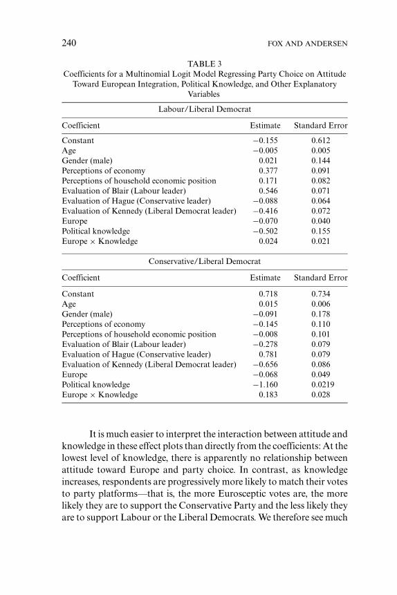
Estimated coefficients and their standard errors from a finalmultinomial logit model fit to the data are shown in Table 3. We have al-ready argued that interpreting coefficients in logit models is not simple,especially in the presence of interactions. Interpretation of the multino-mial logit model is further complicated because the coefficients refer tocontrasts of categories of the response variable with a baseline category.Nonetheless, we can see even from the coefficients that attitude towardEurope was related to party choice and that this relationship differedaccording to level of political knowledge. An analysis of deviance con-firms that the interaction between attitude toward Europe and politicalknowledge is statistically significant. As was the case with the binarylogit model, however, further interpretation is simplified by plotting thisinteraction as an effect display.
Figure 4 shows the relationship between attitude toward Europeand the fitted probability of voting for each of the three parties at theseveral levels of political knowledge (ranging from 0 to 3). An alter-native display, with 95 percent confidence intervals around the fittedprobabilities, appears in Figure 5. A third display, in Figure 6, showsthe response categories in a manner similar to a stacked bar graph.5
5We are grateful to Michael Ornstein for suggesting this display.
240 FOX AND ANDERSEN
TABLE 3Coefficients for a Multinomial Logit Model Regressing Party Choice on Attitude
Toward European Integration, Political Knowledge, and Other ExplanatoryVariables
Labour/Liberal Democrat
Coefficient Estimate Standard Error
Constant −0.155 0.612Age −0.005 0.005Gender (male) 0.021 0.144Perceptions of economy 0.377 0.091Perceptions of household economic position 0.171 0.082Evaluation of Blair (Labour leader) 0.546 0.071Evaluation of Hague (Conservative leader) −0.088 0.064Evaluation of Kennedy (Liberal Democrat leader) −0.416 0.072Europe −0.070 0.040Political knowledge −0.502 0.155Europe × Knowledge 0.024 0.021
Conservative/Liberal Democrat
Coefficient Estimate Standard Error
Constant 0.718 0.734Age 0.015 0.006Gender (male) −0.091 0.178Perceptions of economy −0.145 0.110Perceptions of household economic position −0.008 0.101Evaluation of Blair (Labour leader) −0.278 0.079Evaluation of Hague (Conservative leader) 0.781 0.079Evaluation of Kennedy (Liberal Democrat leader) −0.656 0.086Europe −0.068 0.049Political knowledge −1.160 0.0219Europe × Knowledge 0.183 0.028
It is much easier to interpret the interaction between attitude andknowledge in these effect plots than directly from the coefficients: At thelowest level of knowledge, there is apparently no relationship betweenattitude toward Europe and party choice. In contrast, as knowledgeincreases, respondents are progressively more likely to match their votesto party platforms—that is, the more Eurosceptic votes are, the morelikely they are to support the Conservative Party and the less likely theyare to support Labour or the Liberal Democrats. We therefore see much

EFFECT DISPLAYS FOR LOGIT MODELS 241
2 4 6 8 10
0.0
0.2
0.4
0.6
0.8
1.0
Knowledge = 2
Attitude toward Europe
Fitt
ed p
roba
bilit
y
2 4 6 8 10
0.0
0.2
0.4
0.6
0.8
1.0
Knowledge = 3
Attitude toward Europe
Fitt
ed p
roba
bilit
y
Liberal DemocratLabourConservative
2 4 6 8 10
0.0
0.2
0.4
0.6
0.8
1.0
Knowledge = 0
Attitude toward Europe
Fitt
ed p
roba
bilit
y
2 4 6 8 10
0.0
0.2
0.4
0.6
0.8
1.0
Knowledge = 1
Attitude toward Europe
Fitt
ed p
roba
bilit
y
FIGURE 4. Display of the interaction between attitude toward Europe and political knowl-edge, showing the effects of these variables on the fitted probability of voting foreach of the three major British parties in 2001.
more clearly than we could from Table 3 the importance of informationto voting behavior—issues do matter in elections, but only to those whohave knowledge of party platforms (a point discussed at greater lengthin Andersen 2003).
4. EFFECT DISPLAYS FOR THE PROPORTIONAL-ODDSLOGIT MODEL
4.1. Basic Results
The proportional-odds logit model is a common model for an ordinalresponse variable (e.g., McCullagh and Nelder 1989, chap. 5; Fox 1997,

242 FOX AND ANDERSEN
24
68
10
0.00.20.40.60.81.0
Kn
ow
led
ge
= 0
Labour
24
68
10
0.00.20.40.60.81.0
Kn
ow
led
ge
= 1
24
68
10
0.00.20.40.60.81.0
Kn
ow
led
ge
= 2
24
68
10
0.00.20.40.60.81.0
Kn
ow
led
ge
= 3
24
68
10
0.00.20.40.60.81.0
Conservative
24
68
10
0.00.20.40.60.81.0
24
68
10
0.00.20.40.60.81.0
24
68
10
0.00.20.40.60.81.0
24
68
10
0.00.20.40.60.81.0
Att
itu
de
tow
ard
Eu
rop
e
Liberal Democrat
24
68
10
0.00.20.40.60.81.0
Att
itu
de
tow
ard
Eu
rop
e
24
68
100.00.20.40.60.81.0
Att
itu
de
tow
ard
Eu
rop
e
24
68
10
0.00.20.40.60.81.0
Att
itu
de
tow
ard
Eu
rop
e
FIG
UR
E5.
Alt
erna
tive
disp
lay
ofth
ein
tera
ctio
nbe
twee
nat
titu
deto
war
dE
urop
ean
dpo
litic
alkn
owle
dge.
The
dash
edlin
esgi
vepo
int-
wis
e95
-per
cent
conf
iden
cein
terv
als
arou
ndth
efi
tted
prob
abili
ties
.

EFFECT DISPLAYS FOR LOGIT MODELS 243
2 4 6 8 10
020
4060
8010
0Knowledge = 0
Attitude toward Europe
Per
cent
age
Liberal Democrat
Labour
Conservative
2 4 6 8 10
020
4060
8010
0
Knowledge = 1
Attitude toward Europe
Per
cent
age
Liberal Democrat
Labour
Conservative
2 4 6 8 10
020
4060
8010
0
Knowledge = 2
Attitude toward Europe
Per
cent
age
Liberal Democrat
Labour
Conservative
2 4 6 8 10
020
4060
8010
0Knowledge = 3
Attitude toward Europe
Per
cent
age
Liberal Democrat
Labour
Conservative
FIGURE 6. A third version of the effect display for the interaction between attitude towardEurope and political knowledge.
chap. 15; Long 1997, chap. 5; Powers and Xie 2000, chap. 6). The modelis often motivated as follows: Suppose that there is a continuous, but un-observable, response variable, ξ , which is a linear function of a predictorvector x′ plus a random error:
ξi = β′xi + εi
= ηi + εi
We cannot observe ξ directly, but instead implicitly dissect its range intom class intervals at the (unknown) thresholds α1 < α2 < · · · < αm−1,producing the observed ordinal response variable y. That is,

244 FOX AND ANDERSEN
yi =
1 for ξi ≤ α1
2 for α1 < ξi ≤ α2
...
m − 1 for αm−2 < ξi ≤ αm−1
m for αm−1 < ξi .
.
The cumulative probability distribution of yi is given by
Pr(yi ≤ j ) = Pr(ξi ≤ α j )
= Pr(ηi + εi ≤ α j )
= Pr(εi ≤ α j − ηi )
for j = 1, 2, . . . , m − 1. If the errors ε i are independently distributed ac-cording to the standard logistic distribution, with distribution function
(z) = 11 + e−z
,
then we get the proportional-odds logit model
logit[Pr(yi > j )] = logePr(yi > j )Pr(yi ≤ j )
= −α j + β′xi
(7)
for j = 1,2,. . ., m − 1. (The similar ordered probit model is produced byassuming that the ε i are normally distributed.)
Model 7 is overparametrized: Since the β vector typically in-cludes a constant, say β 1, we have m−1 regression equations, the in-tercepts of which are expressed in terms of m (i.e., one too many)parameters. A solution is to eliminate the constant fromβ. Settingβ 1 =0in this manner in effect establishes the origin of the latent continuumξ ; we already implicitly established the scale of ξ by fixing the varianceof the error to the variance of the standard logistic distribution (π2/3).For convenience, we will absorb the negative sign into the intercept,

EFFECT DISPLAYS FOR LOGIT MODELS 245
rewriting the model as
logit[Pr(yi > j )] = α j + β′xi , for j = 1, 2, . . . , m − 1.
The thresholds are then the negatives of the intercepts α j. Because fittedprobabilities under the model are unaffected by this reparametrization,effect displays are invariant as well.
The proportional-odds model is more parsimonious than themultinomial logit model (and other models for unordered polytomies):While the proportional-odds model has m + p −2 independent param-eters, the multinomial logit model has p(m−1) independent parameters.Of course, the proportional-odds model is also less flexible, and maynot adequately represent the data.
We propose two strategies for constructing effect displays for theproportional-odds model. The more straightforward strategy is to ploton the scale of the latent continuum, using the estimated thresholds,−α̂ j, to show the division of the continuum into ordered categories.There is not much more to say about this approach, since—other thanmarking the thresholds (as illustrated in the example in Section 4.2)—one proceeds exactly as for a linear model.
The second approach is to display fitted probabilities of categorymembership, as we did for the multinomial logit model. Suppose thatwe need the fitted probabilities at x′
0 (where the constant regressor hasbeen removed from the design vector x′, and the intercept from theparameter vector β). Let η0 = x′
0β, and let µ0 j = Pr(Y0 = j ). Then
µ01 = 11 + exp(α1 + η0)
µ0 j = exp(η0)[exp(α j−1) − exp(α j )
][1 + exp(α j−1 + η0)
] [1 + exp(α j + η0)
] , j = 2, . . . , m − 1
µ0m = 1 −m−1∑j=1
µ0 j
As in the case of the multinomial logit model, we derive approximatestandard errors by the delta method. The necessary derivatives aremessier here, however:

246 FOX AND ANDERSEN
∂µ01
∂α1= − exp(α1 + η0)
[1 + exp(α1 + η0)]2
∂µ01
∂α j= 0, j = 2, . . . , m − 1
∂µ01
∂β= − exp(α1 + η0)x0
[1 + exp(α1 + η0)]2
∂µ0 j
∂α j−1= exp(α j−1 + η0)[
1 + exp(α j−1 + η0)]2
∂µ0 j
∂α j= − exp(α j + η0)[
1 + exp(α j + η0)]2
∂µ0 j
∂α j ′= 0, j ′ �= j, j − 1
∂µ0 j
∂β= exp(η0)
[exp(α j ) − exp(α j−1)
] [exp(α j−1 + α j + 2η0) − 1
]x0[
1 + exp(α j−1 + η0)]2 [
1 + exp(α j + η0)]2
∂µ0m
∂αm−1= exp(αm−1 + η0)
[1 + exp(αm−1 + η0)]2
∂µ0m
∂α j= 0, j = 1, . . . , m − 2
∂µ0m
∂β= exp(αm−1 + η0)x0
[1 + exp(αm−1 + η0)]2.
Let us stack up all of the parameters in the vector γ = (α1, . . ., αm−1,
β′)′, and let
V̂ (γ̂) = [vst] , s, t = 1, . . . , r,
where r = m + p − 2. Then, as for the multinomial logit model,
V̂ (µ̂0 j ) r∑
s=1
r∑t=1
vst∂µ̂0 j
∂γ̂s
∂µ̂0 j
∂γ̂t
and
V̂ (λ̂0 j ) 1
µ̂ 20 j (1 − µ̂0 j )2
V̂ (µ̂0 j ),
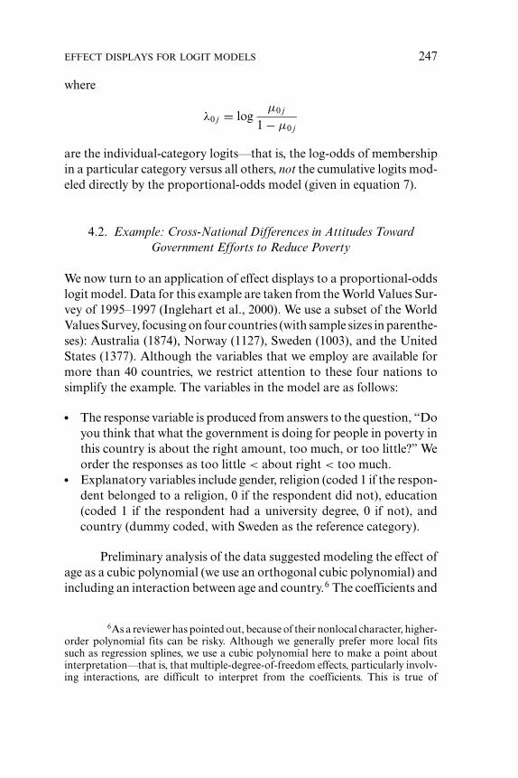
EFFECT DISPLAYS FOR LOGIT MODELS 247
where
λ0 j = logµ0 j
1 − µ0 j
are the individual-category logits—that is, the log-odds of membershipin a particular category versus all others, not the cumulative logits mod-eled directly by the proportional-odds model (given in equation 7).
4.2. Example: Cross-National Differences in Attitudes TowardGovernment Efforts to Reduce Poverty
We now turn to an application of effect displays to a proportional-oddslogit model. Data for this example are taken from the World Values Sur-vey of 1995–1997 (Inglehart et al., 2000). We use a subset of the WorldValues Survey, focusing on four countries (with sample sizes in parenthe-ses): Australia (1874), Norway (1127), Sweden (1003), and the UnitedStates (1377). Although the variables that we employ are available formore than 40 countries, we restrict attention to these four nations tosimplify the example. The variables in the model are as follows:
� The response variable is produced from answers to the question, “Doyou think that what the government is doing for people in poverty inthis country is about the right amount, too much, or too little?” Weorder the responses as too little < about right < too much.
� Explanatory variables include gender, religion (coded 1 if the respon-dent belonged to a religion, 0 if the respondent did not), education(coded 1 if the respondent had a university degree, 0 if not), andcountry (dummy coded, with Sweden as the reference category).
Preliminary analysis of the data suggested modeling the effect ofage as a cubic polynomial (we use an orthogonal cubic polynomial) andincluding an interaction between age and country.6 The coefficients and
6As a reviewer has pointed out, because of their nonlocal character, higher-order polynomial fits can be risky. Although we generally prefer more local fitssuch as regression splines, we use a cubic polynomial here to make a point aboutinterpretation—that is, that multiple-degree-of-freedom effects, particularly involv-ing interactions, are difficult to interpret from the coefficients. This is true of

248 FOX AND ANDERSEN
TABLE 4Coefficients for a Proportional-Odds Logit Model Regressing Attitude Toward
Government Efforts to Help People in Poverty on Gender, Age, Religion,Education, and Country
Coefficient Estimate Standard Error
Gender (male) 0.169 0.053Religion (yes) −0.168 0.078University degree (yes) 0.141 0.067Age (linear) 10.659 5.404Age (quadratic) 7.535 6.245Age (cubic) 8.887 6.663Norway 0.250 0.087Australia 0.572 0.823USA 1.176 0.087Norway × Age (linear) −7.905 7.091Australia × Age (linear) 9.264 6.312USA × Age (linear) 10.868 6.647Norway × Age (quadratic) −0.625 8.027Australia × Age (quadratic) −17.716 7.034USA × Age (quadratic) −7.692 7.352Norway × Age (cubic) 0.485 8.568Australia × Age (cubic) −2.762 7.385USA × Age (cubic) −11.163 7.587ThresholdsToo little | about right 0.449 0.106About right | too much 2.262 0.111
aAge is represented in the model by a cubic orthogonal polynomial, and interactionsbetween age and country are included in the model.
their standard errors from a final model fit to the data are displayed inTable 4.
The complexity of the nonlinear trend for age, its interaction withcountry, and coefficients for cumulative logits make it extremely diffi-cult to interpret the parameter estimates associated with age. Instead, weconstruct effect displays for the interaction of age with country. Figure 7plots fitted probabilities for each category of the response variable
orthogonal polynomials, as used here, of ordinary polynomials (which provide thesame fit to the data), and of regression splines. In fact, the cubic fit that we haveemployed represents the data well, and provides results similar to a regression spline.See Hastie and Tibshirani (1990, sec. 2.9) for a good discussion of regression splinesand their general advantages relative to polynomial regression.

EFFECT DISPLAYS FOR LOGIT MODELS 249
20 30 40 50 60 70 80 90
0.0
0.2
0.4
0.6
0.8
1.0
Sweden
Age
Fitt
ed p
roba
bilit
y
Too littleAbout rightToo much
20 30 40 50 60 70 80 90
0.0
0.2
0.4
0.6
0.8
1.0
Norway
Age
Fitt
ed p
roba
bilit
y
20 30 40 50 60 70 80 90
0.0
0.2
0.4
0.6
0.8
1.0
Australia
Age
Fitt
ed p
roba
bilit
y
20 30 40 50 60 70 80 90
0.0
0.2
0.4
0.6
0.8
1.0
United States
Age
Fitt
ed p
roba
bilit
y
FIGURE 7. Display of the interaction between age and country, showing the effects of thesevariables on attitude toward government efforts to help people in poverty; thegraphs indicate the fitted probability for each of the three categories of the re-sponse variable.
in the same manner as for the multinomial logit model of Section 2.2.Because country takes on only four values while age is continuous, weconstruct a separate plot for each country, placing age on the horizontalaxis. There are three fitted lines in each plot—representing the fittedprobability of choosing each response category. Figure 8 is generallysimilar, but with 95 percent point-wise confidence intervals around thefitted probabilities (and separate panels for each response category, soas not to clutter the plots). Figure 9 shows an alternative display withstacked response categories.
Although the graphs in Figures 7–9 are informative—we see, forexample, that age differences are relatively muted in the United States

250 FOX AND ANDERSEN
2030
4050
6070
80
0.00.20.40.60.81.0
Sw
eden
Too little
2030
4050
6070
80
0.00.20.40.60.81.0
No
rway
2030
4050
6070
80
0.00.20.40.60.81.0
Au
stra
lia
2030
4050
6070
80
0.00.20.40.60.81.0
Un
ited
Sta
tes
2030
4050
6070
80
0.00.20.40.60.81.0
About right
2030
4050
6070
80
0.00.20.40.60.81.0
2030
4050
6070
80
0.00.20.40.60.81.0
2030
4050
6070
80
0.00.20.40.60.81.0
2030
4050
6070
80
0.00.20.40.60.81.0
Ag
e
Too much
2030
4050
6070
80
0.00.20.40.60.81.0
Ag
e
2030
4050
6070
800.00.20.40.60.81.0
Ag
e
2030
4050
6070
80
0.00.20.40.60.81.0
Ag
e
FIG
UR
E8.
Dis
play
ofth
ein
tera
ctio
nbe
twee
nag
ean
dco
untr
y,sh
owin
gpo
int-
wis
e95
perc
ent
conf
iden
cein
terv
als
arou
ndth
efi
tted
prob
abili
ties
.

EFFECT DISPLAYS FOR LOGIT MODELS 251
20 30 40 50 60 70 80
020
4060
8010
0Sweden
Age
Per
cent
age
Too little
About right
Too much
20 30 40 50 60 70 80
020
4060
8010
0
Norway
Age
Per
cent
age
Too little
About right
Too much
20 30 40 50 60 70 80
020
4060
8010
0
Australia
Age
Per
cent
age
Too little
About right
Too much
20 30 40 50 60 70 80
020
4060
8010
0
United States
Age
Per
cent
age
Too little
About right
Too much
FIGURE 9. Alternative effect display of the interaction between age and country.
and that respondents there are less likely than others to feel that thegovernment is not doing enough for the poor—the displays do not takefull advantage of the parsimony of the proportional-odds model. Wecan capitalize on the structure of the proportional-odds model to plotthe fitted response on the scale of the latent attitude continuum. Wepursue this strategy in Figure 10, in which there is only one line foreach country.7 The estimated thresholds from the proportional-oddsmodel are displayed as horizontal lines, dividing the latent continuuminto three categories. Notice that none of the fitted curves exceeds the
7Abstract versions of Figure 10 are often used to explain the proportional-odds model (e.g., see Agresti 1990, fig. 9.2), but not typically to present the resultsof fitting the model to data and not for the kind of partial-effect plot developed inthis paper.


EFFECT DISPLAYS FOR LOGIT MODELS 253
5. DISCUSSION
Statistical models for polytomous response variables are increasinglyemployed in social research. Too frequently, however, the results of fit-ting these models are described perfunctorily. Efforts to ensure carefulmodel specification can be largely wasted if the results are not conveyedclearly. Although it is difficult to interpret the coefficients of complexstatistical models that transform response probabilities nonlinearly, sim-ply discussing their signs and statistical significance tells us little aboutthe structure of the data. The approach described and illustrated inthis paper, in contrast, goes a long way toward clarifying the fit ofmultinomial logit and proportional-odds models and simplifying theirinterpretation.
Effect displays allow us to visualize key portions of the responsesurface of a statistical model, and thus to understand better how ex-planatory variables combine to influence the response. The computationof effect displays for models of polytomous response variables is fairlystraightforward and can be implemented in most statistical software.Computations associated with standard errors and confidence intervalsfor these effect displays are more difficult, however. We intend to extendthe effects package for R (described in Fox 2003) to cover multino-mial and proportional-odds logit models, making the construction ofeffect displays for these models essentially automatic. Until that time, aprogram described in the appendix to this paper may be employed forcomputing effects, their standard errors, and confidence limits.
APPENDIX: COMPUTING
Fitted values and their standard errors for effect displays may be com-puted with an R function (program), polytomousEffects, availableon the web at <http://socserv.socsci.mcmaster.ca/jfox/Papers/polytomous-effect-displays.html>. Also available are code and datafor the examples in this paper. R (Ihaka and Gentleman, 1996; R De-velopment Core Team, 2004) is a free, open-source implementation ofthe S statistical computing environment now in widespread use, par-ticularly among statisticians. The polytomousEffects function usesthe strategy for safe prediction described in Hastie (1992, sec. 7.3.3) toensure that fitted values are computed correctly in models with terms

254 FOX AND ANDERSEN
(such as orthogonal polynomials and B-splines) whose basis dependsupon the data.
REFERENCES
Agresti, A. 1990. Categorical Data Analysis. New York: Wiley.Andersen, R. 2003. “Do Newspapers Enlighten Preferences? Personal Ideology,
Party Choice, and the Electoral Cycle: The United Kingdom, 1992–97.” Cana-dian Journal of Political Science 36:601–20.
Andersen, R., A. Heath, and R. Sinnott. 2002. “Political Knowledge and ElectoralChoice.” British Elections and Parties Review 12:11–27.
Andersen, R., J. Tilley, and A. Heath. 2005. “Political Knowledge and EnlightenedPreferences.” British Journal of Political Science 35:285–303.
Firth, D. 1991. “Generalized Linear Models.” Pp. 55–82 in Statistical Theory andModeling: In Honour of Sir David Cox, FRS edited by D. V. Hinkley, N. Reid,and E. J. Snell. London: Chapman and Hall.
Fisher, R. A. 1936. Statistical Methods for Research Workers, 6th ed. Edinburgh:Oliver and Boyd.
Fox, J. 1987. “Effect Displays for Generalized Linear Models.” Pp. 347–61 in Socio-logical Methodology, vol. 17, edited by C. C. Clogg. Washington, DC: AmericanSociological Association.
—— 1997. Applied Regression Analysis, Linear Models, and Related Methods. Thou-sand Oaks, CA: Sage.
—— 2003. “Effect Displays in R for Generalised Linear Models.” Journal of Sta-tistical Software 8(15):1–27.
Goodnight, J. H., and W. R. Harvey. 1978. “Least Squares Means in the Fixed-Effect General Linear Model.” Technical Report No. R-103. Cary, NC: SASInstitute.
Hastie, T. J. 1992. “Generalized Additive Models.” Pp. 249–307 in Statistical Modelsin S edited by J. M. Chambers and T. J. Hastie. Pacific Grove, CA: Wadsworth.
Hastie, T. J., and R. J. Tibshirani. 1990. Generalized Additive Models. London:Chapman and Hall.
Hastie, T., R. Tibshirani, and J. Friedman. 2001. The Elements of Statistical Learn-ing: Data Mining, Inference, and Prediction. New York: Springer.
Ihaka, R., and R. Gentleman. 1996. “R: A Language for Data Analysis and Graph-ics.” Journal of Computational and Graphical Statistics 5:299–314.
Inglehart, R. E. A. 2000. World values surveys and European value surveys, 1981–1984:1990–1993, and 1995–1997 [computer file]. Ann Arbor, MI: Institute forSocial Research [producer], Inter–University Consortium for Political and SocialResearch [distributor].
King, G., M. Tomz, and J. Wittenberg. 2000. “Making the Most of Statistical Anal-yses: Improving Interpretation and Presentation.” American Journal of PoliticalScience 44:347–61.
Long, J. S. 1997. Regression Models for Categorical and Limited Dependent Variables.Thousand Oaks, CA: Sage.

EFFECT DISPLAYS FOR LOGIT MODELS 255
McCullagh, P., and J. A. Nelder. 1989. Generalized Linear Models. 2d ed. London:Chapman and Hall.
Nelder, J. A. 1977. “A Reformulation of Linear Models” (with commentary). Jour-nal of the Royal Statistical Society, Series A, 140:48–76.
Powers, D. A., and Y. Xie. 2000. Statistical Methods for Categorical Data Analysis.San Diego: Academic Press.
R Core Development Team. 2004. R: A Language and Environment for StatisticalComputing. Vienna: R Foundation for Statistical Computing.
Rao, C. R. 1965. Linear Statistical Inference and Its Applications. New York: Wiley.Searle, S. R., F. M. Speed, and G. A. Milliken. 1980. “Population Marginal Means
in the Linear Model: An Alternative to Least Squares Means.” The AmericanStatistician 34:216–21.
Tomz, M., J. Wittenberg, and G. King. 2003. “Clarify: Software for Interpretingand Presenting Statistical Results.” Journal of Statistical Software 8:1–29.
Weisberg, S. 2005. Applied Linear Regression. 3d ed. New York: Wiley.